AI-IMU Dead-Reckoning
Abstract
In this paper we propose a novel accurate method for dead-reckoning of wheeled vehicles based only on an Inertial Measurement Unit (IMU). In the context of intelligent vehicles, robust and accurate dead-reckoning based on the IMU may prove useful to correlate feeds from imaging sensors, to safely navigate through obstructions, or for safe emergency stops in the extreme case of exteroceptive sensors failure. The key components of the method are the Kalman filter and the use of deep neural networks to dynamically adapt the noise parameters of the filter. The method is tested on the KITTI odometry dataset, and our dead-reckoning inertial method based only on the IMU accurately estimates 3D position, velocity, orientation of the vehicle and self-calibrates the IMU biases. We achieve on average a 1.10% translational error and the algorithm competes with top-ranked methods which, by contrast, use LiDAR or stereo vision. We make our implementation open-source at:
Index Terms:
localization, deep learning, invariant extended Kalman filter, KITTI dataset, inertial navigation, inertial measurement unitI Introduction
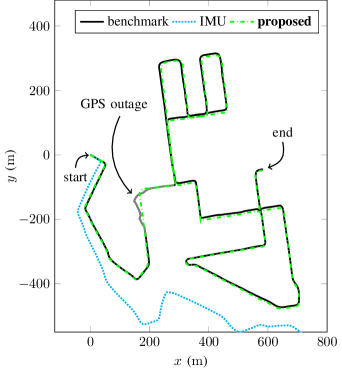
Intelligent vehicles need to know where they are located in the environment, and how they are moving through it. An accurate estimate of vehicle dynamics allows validating information from imaging sensors such as lasers, ultrasonic systems, and video cameras, correlating the feeds, and also ensuring safe motion throughout whatever may be seen along the road [1]. Moreover, in the extreme case where an emergency stop must be performed owing to severe occlusions, lack of texture, or more generally imaging system failure, the vehicle must be able to assess accurately its dynamical motion. For all those reasons, the Inertial Measurement Unit (IMU) appears as a key component of intelligent vehicles [2]. Note that Global Navigation Satellite System (GNSS) allows for global position estimation but it suffers from phase tracking loss in densely built-up areas or through tunnels, is sensitive to jamming, and may not be used to provide continuous accurate and robust localization information, as exemplified by a GPS outage in the well known KITTI dataset [3], see Figure 1.
Kalman filters are routinely used to integrate the outputs of IMUs. When the IMU is mounted on a car, it is common practice to make the Kalman filter incorporate side information about the specificity of wheeled vehicle dynamics, such as approximately null lateral and upward velocity assumption in the form of pseudo-measurements. However, the degree of confidence the filter should have in this side information is encoded in a covariance noise parameter which is difficult to set manually, and moreover which should dynamically adapt to the motion, e.g., lateral slip is larger in bends than in straight lines. Using the recent tools from the field of Artificial Intelligence (AI), namely deep neural networks, we propose a method to automatically learn those parameters and their dynamic adaptation for IMU only dead-reckoning. Our contributions, and the paper’s organization, are as follows:
-
•
we introduce a state-space model for wheeled vehicles as well as simple assumptions about the motion of the car in Section II;
-
•
we implement a state-of-the-art Kalman filter [4, 5] that exploits the kinematic assumptions and combines them with the IMU outputs in a statistical way in Section III-C. It yields accurate estimates of position, orientation and velocity of the car, as well as IMU biases, along with associated uncertainty (covariance);
- •
-
•
we demonstrate the performances of the approach on the KITTI dataset [3] in Section V. Our approach solely based on the IMU produces accurate estimates and competes with top-ranked LiDAR and stereo camera methods [6, 7]; and we do not know of IMU based dead-reckoning methods capable to compete with such results;
-
•
the approach is not restricted to inertial only dead-reckoning of wheeled vehicles. Thanks to the versatility of the Kalman filter, it can easily be applied for railway vehicles [8], coupled with GNSS, the backbone for IMU self-calibration, or for using IMU as a speedometer in path-reconstruction and map-matching methods [9, 10, 11, 12].
I-A Relation to Previous Literature
Autonomous vehicle must robustly self-localize with their embarked sensor suite which generally consists of odometers, IMUs, radars or LiDARs, and cameras [2, 12, 1]. Simultaneous Localization And Mapping based on inertial sensors, cameras, and/or LiDARs have enabled robust real-time localization systems, see e.g., [7, 6]. Although these highly accurate solutions based on those sensors have recently emerged, they may drift when the imaging system encounters troubles.
As concerns wheeled vehicles, taking into account vehicle constraints and odometer measurements are known to increase the robustness of localization systems [13, 14, 15, 16]. Although quite successful, such systems continuously process a large amount of data which is computationally demanding and energy consuming. Moreover, an autonomous vehicle should run in parallel its own robust IMU-based localization algorithm to perform maneuvers such as emergency stops in case of other sensors failures, or as an aid for correlation and interpretation of image feeds [2].
High precision aerial or military inertial navigation systems achieve very small localization errors but are too costly for consumer vehicles. By contrast, low and medium-cost IMUs suffer from errors such as scale factor, axis misalignment and random walk noise, resulting in rapid localization drift [17]. This makes the IMU-based positioning unsuitable, even during short periods.
Inertial navigation systems have long leveraged virtual and pseudo-measurements from IMU signals, e.g. the widespread Zero velocity UPdaTe (ZUPT) [18, 19, 20], as covariance adaptation [21]. In parallel, deep learning and more generally machine learning are gaining much interest for inertial navigation [22, 23]. In [22] velocity is estimated using support vector regression whereas [23] use recurrent neural networks for end-to-end inertial navigation. Those methods are promising but restricted to pedestrian dead-reckoning since they generally consider slow horizontal planar motion, and must infer velocity directly from a small sequence of IMU measurements, whereas we can afford to use larger sequences. A more general end-to-end learning approach is [24], which trains deep networks end-to-end in a Kalman filter. Albeit promising, the method obtains large translational error in their stereo odometry experiment. Finally, [25] uses deep learning for estimating covariance of a local odometry algorithm that is fed into a global optimization procedure, and in [26] we used Gaussian processes to learn a wheel encoders error. Our conference paper [20] contains preliminary ideas, albeit not concerned at all with covariance adaptation: a neural network essentially tries to detect when to perform ZUPT.
Dynamic adaptation of noise parameters in the Kalman filter is standard in the tracking literature [27], however adaptation rules are application dependent and are generally the result of manual “tweaking” by engineers. Finally, in [28] the authors propose to use classical machine learning techniques to to learn static noise parameters (without adaptation) of the Kalman filter, and apply it to the problem of IMU-GNSS fusion.
II IMU and Problem Modelling
An inertial navigation system uses accelerometers and gyros provided by the IMU to track the orientation , velocity and position of a moving platform relative to a starting configuration . The orientation is encoded in a rotation matrix whose columns are the axes of a frame attached to the vehicle.
II-A IMU Modelling
The IMU provides noisy and biased measurements of the instantaneous angular velocity vector and specific acceleration as follows [17]
| (1) | ||||
| (2) |
where , are quasi-constant biases and , are zero-mean Gaussian noises. The biases follow a random walk
| (3) | ||||
| (4) |
where , are zero-mean Gaussian noises.
The kinematic model is governed by the following equations
| (5) | ||||
| (6) | ||||
| (7) |
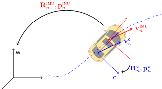
between two discrete time instants sampling at , where we let the IMU velocity be and its position in the world frame. is the rotation matrix that represents the IMU orientation, i.e. that maps the IMU frame to the world frame, see Figure 2. Finally denotes the skew symmetric matrix associated with cross product with . The true angular velocity and the true specific acceleration are the inputs of the system (5)-(7). In our application scenarios, the effects of earth rotation and Coriolis acceleration are ignored, Earth is considered flat, and the gravity vector is a known constant.
All sources of error displayed in (1) and (2) are harmful since a simple implementation of (5)-(7) leads to a triple integration of raw data, which is much more harmful that the unique integration of differential wheel speeds [12]. Indeed, a bias of order has an impact of order on the position after seconds, leading to potentially huge drift.
II-B Problem Modelling
We distinguish between three different frames, see Figure 2: ) the static world frame, ; ) the IMU frame, , where (1)-(2) are measured; and ) the car frame, . The car frame is an ideal frame attached to the car, that will be estimated online and plays a key role in our approach. Its orientation w.r.t. is denoted and its origin denoted is the car to IMU level arm. In the rest of the paper, we tackle the following problem:
IMU Dead-Reckoning Problem.
Given an initial known configuration , perform in real-time IMU dead-reckoning, i.e. estimate the IMU and car variables
| (8) |
using only the inertial measurements and .
III Kalman Filtering with Pseudo-Measurements
The Extended Kalman Filter (EKF) was first implemented in the Apollo program to localize the space capsule, and is now pervasively used in the localization industry, the radar industry, and robotics. It starts from a dynamical discrete-time non-linear law of the form
| (9) |
where denotes the state to be estimated, is an input, and is the process noise which is assumed Gaussian with zero mean and covariance matrix . Assume side information is in the form of loose equality constraints is available. It is then customary to generate a fictitious observation from the constraint function:
| (10) |
and to feed the filter with the information that (pseudo-measurement) as first advocated by [29], see also [13, 30] for application to visual inertial localization and general considerations. The noise is assumed to be a centered Gaussian where the covariance matrix is set by the user and reflects the degree of validity of the information: the larger the less confidence is put in the information.
Starting from an initial Gaussian belief about the state, where represents the initial estimate and the covariance matrix the uncertainty associated to it, the EKF alternates between two steps. At the propagation step, the estimate is propagated through model (9) with noise turned off, , and the covariance matrix is updated through
| (11) |
where , are Jacobian matrices of with respect to and . At the update step, pseudo-measurement is taken into account, and Kalman equations allow to update the estimate and its covariance matrix accordingly.
To implement an EKF, the designer needs to determine the functions and , and the associated noise matrices and . In this paper, noise parameters and will be wholly learned by a neural network.
III-A Defining the Dynamical Model
We now need to assess the evolution of state variables (8). The evolution of , , , and is already given by the standard equations (3)-(7). The additional variables and represent the car frame with respect to the IMU. This car frame is rigidly attached to the car and encodes an unknown fictitious point where the pseudo-measurements of Section III-B are most advantageously made. As IMU is also rigidly attached to the car, and , represent misalignment between IMU and car frame, they are approximately constant
| (12) | ||||
| (13) |
where we let , be centered Gaussian noises with small covariance matrices , that will be learned during training. Noises and encode possible small variations through time of level arm due to the lack of rigidity stemming from dampers and shock absorbers.
III-B Defining the Pseudo-Measurements
Consider the different frames depicted on Figure 2. The velocity of the origin point of the car frame, expressed in the car frame, writes
| (14) |
from basic screw theory, where is the car to IMU level arm. In the car frame, we consider that the car lateral and vertical velocities are roughly null, that is, we generate two scalar pseudo observations of the form (10) that is,
| (15) |
where the noises are assumed centered and Gaussian with covariance matrix . The filter is then fed with the pseudo-measurement that .
Assumptions that and are roughly null are common for cars moving forward on human made roads or wheeled robots moving indoor. Treating them as loose constraints, i.e., allowing the uncertainty encoded in to be non strictly null, leads to much better estimates than treating them as strictly null [13].
It should be duly noted the vertical velocity is expressed in the car frame, and thus the assumption it is roughly null generally holds for a car moving on a road even if the motion is 3D. It is quite different from assuming null vertical velocity in the world frame, which then boils down to planar horizontal motion.
The main point of the present work is that the validity of the null lateral and vertical velocity assumptions widely vary depending on what maneuver is being performed: for instance, is much larger in turns than in straight lines. The role of the noise parameter adapter of Section IV-A, based on AI techniques, will be to dynamically assess the parameter that reflects confidence in the assumptions, as a function of past and present IMU measurements.
III-C The Invariant Extended Kalman Filter (IEKF)
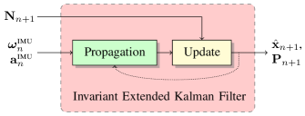
For inertial navigation, we advocate the use of a recent EKF variant, namely the Invariant Extended Kalman Filter (IEKF), see [4, 5], that has recently given raise to a commercial aeronautics product [31] and to various successes in the field of visual inertial odometry [32, 33, 34]. We thus opt for an IEKF to perform the fusion between the IMU measurements (1)-(2) and (15) treated as pseudo-measurements. Its architecture, which is identical to the conventional EKF’s, is recapped in Figure 3.
However, understanding in detail the IEKF [4] requires some background in Lie group geometry. The interested reader is referred to the Appendix where the exact equations are provided.
IV Proposed AI-IMU Dead-Reckoning
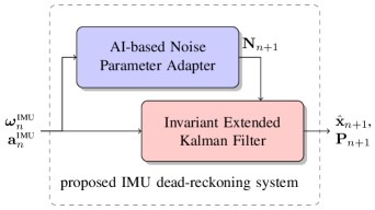
This section describes our system for recovering all the variables of interest from IMU signals only. Figure 4 illustrates the approach which consists of two main blocks summarized as follows:
- •
- •
The amplitude of process noise parameters are considered fixed by the algorithm, and are learned during training.
Note that the adapter computes covariances meant to improve localization accuracy, and thus the computed values may broadly differ from the actual statistical covariance of (15), see Section V-D for more details. In this respect, our approach is related to [24] but the considered problem is more challenging: our state-space is of dimension 21 whereas [24] has a state-space of dimension only 3. Moreover, we compare our results in the sequel to state-of-the-art methods based on stereo cameras and LiDARs, and we show we may achieve similar results based on the moderately precise IMU only.
IV-A AI-based Measurement Noise Parameter Adapter
The measurement noise parameter adapter computes at each instant the covariance used in the filter update, see Figure 3. The base core of the adapter is a Convolutional Neural Network (CNN) [35]. The networks takes as input a window of inertial measurements and computes
| (16) |
Our motivations for the above simple CNN-like architecture are threefold:
-
)
avoiding over-fitting by using a relatively small number of parameters in the network and also by making its outputs independent of state estimates;
-
)
obtaining an interpretable adapter from which one can infer general and safe rules using reverse engineering, e.g. to which extent must one inflate the covariance during turns, for e.g., generalization to all sorts of wheeled and commercial vehicles, see Section V-D;
- )
The complete architecture of the adapter consists of a bunch of CNN layers followed by a full layer outputting a vector . The covariance is then computed as
| (17) |
with , and where and correspond to our initial guess for the noise parameters. The network thus may inflate covariance up to a factor and squeeze it up to a factor with respect to its original values. Additionally, as long as the network is disabled or barely reactive (e.g. when starting training), we get and recover the initial covariance .
Regarding process noise parameter , we choose to fix it to a value and leave its dynamic adaptation for future work. However its entries are optimized during training, see Section IV-C.
IV-B Implementation Details
We provide in this section the setting and the implementation details of our method. We implement the full approach in Python with the PyTorch111https://pytorch.org/ library for the noise parameter adapter part. We set as initial values before training
| (18) | ||||
| (19) | ||||
| (20) |
where , , , , , , in the initial error covariance , , , , , , for the noise propagation covariance matrix , , and for the measurement covariance matrix. The zero values in the diagonal of in (18) corresponds to a perfect prior of the initial yaw, position and zero vertical speed.
The adapter is a 1D temporal convolutional neural network with 2 layers. The first layer has kernel size 5, output dimension 32, and dilatation parameter 1. The second has kernel size 5, output dimension 32 and dilatation parameter 3, thus it set the window size equal to . The CNN is followed by a fully connected layer that output the scalars and . Each activation function between two layers is a ReLU unit [35]. We define in the right part of (17) which allows for each covariance element to be higher or smaller than its original values.
IV-C Training
We seek to optimize the relative translation error computed from the filter estimates , which is the averaged increment error for all possible sub-sequences of length to .
Toward this aim, we first define the learnable parameters. It consists of the 6210 parameters of the adapter, along with the parameter elements of and in (18)-(19), which add 12 parameters to learn. We then choose an Adam optimizer [36] with learning rate that updates the trainable parameters. Training consists of repeating for a chosen number of epochs the following iterations:
-
)
sample a part of the dataset;
-
)
get the filter estimates for then computing loss and gradient w.r.t. the learnable parameters;
-
)
update the learnable parameters with gradient and optimizer.
Following continual training [37], we suppose the number of epochs is huge, potentially infinite (in our application we set this number to 400). This makes sense for online training in a context where the vehicle gathers accurate ground-truth poses from e.g. its LiDAR system or precise GNSS. It requires careful procedures for avoiding over-fitting, such that we use dropout and data augmentation [35]. Dropout refers to ignoring units of the adapter during training, and we set the probability of any CNN element to be ignored (set to zero) during a sequence iteration.
| test seq. | environment | IMLS [6] | ORB-SLAM2 [7] | IMU | proposed | ||||||
| length | duration | ||||||||||
| () | () | (%) | () | (%) | () | (%) | () | (%) | () | ||
| 01 | 2.6 | 110 | highway | 0.48 | 0.08 | 1.38 | 0.20 | 5.35 | 0.12 | 1.11 | 0.12 |
| 03 | - | 80 | country | - | - | - | - | - | - | - | - |
| 04 | 0.4 | 27 | country | 0.25 | 0.08 | 0.41 | 0.21 | 0.97 | 0.10 | 0.35 | 0.08 |
| 06 | 1.2 | 110 | urban | 0.78 | 0.07 | 0.89 | 0.22 | 5.78 | 0.19 | 0.97 | 0.20 |
| 07 | 0.7 | 110 | urban | 0.32 | 0.12 | 1.16 | 0.49 | 12.6 | 0.30 | 0.84 | 0.32 |
| 08 | 3.2 | 407 | urban, country | 1.84 | 0.17 | 1.52 | 0.30 | 549 | 0.56 | 1.48 | 0.32 |
| 09 | 1.7 | 159 | urban, country | 0.97 | 0.11 | 1.01 | 0.25 | 23.4 | 0.32 | 0.80 | 0.22 |
| 10 | 0.9 | 120 | urban, country | 0.50 | 0.14 | 0.31 | 0.34 | 4.58 | 0.25 | 0.98 | 0.23 |
| average scores | 0.98 | 0.12 | 1.17 | 0.27 | 171 | 0.31 | 1.10 | 0.23 | |||
Regarding ), we sample a batch of nine sequences, where each sequence starts at a random arbitrary time. We add to data a small Gaussian noise with standard deviation , a.k.a. data augmentation technique. We compute ) with standard backpropagation, and we finally clip the gradient norm to a maximal value of to avoid gradient explosion at step ).
We stress the loss function consists of the relative translation error , i.e. we optimize parameters for improving the filter accuracy, disregarding the values actually taken by , in the spirit of [24].
V Experimental Results
We evaluate the proposed method on the KITTI dataset [3], which contains data recorded from LiDAR, cameras and IMU, along with centimeter accurate ground-truth pose from different environments (e.g., urban, highways, and streets). The dataset contains 22 sequences for benchmarking odometry algorithms, 11 of them contain publicly available ground-truth trajectory, raw and synchronized IMU data. We download the raw data with IMU signals sampled at () rather than the synchronized data sampled at , and discard seq. 03 since we did not find raw data for this sequence. The RT3003222https://www.oxts.com/ IMU has announced gyro and accelerometer bias stability of respectively and . The KITTI dataset has an online benchmarking system that ranks algorithms. However we could not submit our algorithm for online ranking since sequences used for ranking do not contain IMU data, which is reserved for training only. Our implementation is made open-source at:
V-A Evaluation Metrics and Compared Methods
To assess performances we consider the two error metrics proposed in [3]:
V-A1 Relative Translation Error ()
which is the averaged relative translation increment error for all possible sub-sequences of length , …, , in percent of the traveled distance;
V-A2 Relative Rotational Error ()
that is the relative rotational increment error for all possible sub-sequences of length , …, , in degree per meter.
We compare four methods which alternatively use LiDAR, stereo vision, and IMU-based estimations:
-
•
IMLS [6]: a recent state-of-the-art LiDAR-based approach ranked 3rd in the KITTI benchmark. The author provided us with the code after disabling the loop-closure module;
-
•
ORB-SLAM2 [7]: a popular and versatile library for monocular, stereo and RGB-D cameras that computes a sparse reconstruction of the map. We took the open-source code, disable loop-closure capability and evaluate the stereo algorithm without modifying any parameter;
- •
-
•
proposed: the proposed approach, that uses only the IMU signals and involves no other sensor.
V-B Trajectory Results
We follow the same protocol for evaluating each sequence: ) we initialize the filter with parameters described in Section IV-B; ) we train then the noise parameter adapter following Section IV-C for 400 epochs without the evaluated sequence (e.g. for testing seq. 10, we train on seq. 00-09) so that the noise parameter has never been confronted with the evaluated sequence; ) we run the IMU-based methods on the full raw sequence with ground-truth initial configuration (), whereas we initialize remaining variables at zero (, ); and ) we get the estimates only on time corresponding to the odometry benchmark sequence. LiDAR and visual methods are directly evaluated on the odometry sequences.
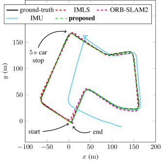
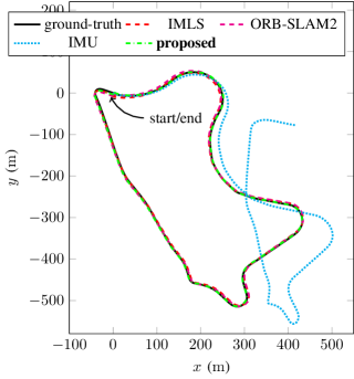
Results are averaged in Table 1 and illustrated in Figures 1, 5 and 6, where we exclude sequences 00, 02 and 05 which contain problems with the data, and will be discussed separately in Section V-C. From these results, we see that:
-
•
LiDAR and visual methods perform generally well in all sequences, and the LiDAR method achieves slightly better results than its visual counterpart;
-
•
our method competes on average with the latter image based methods, see Table 1;
-
•
directly integrating the IMU signals leads to rapid drift of the estimates, especially for the longest sequences but even for short periods;
-
•
Our method looks unaffected by stops of the car, as in seq. 07, see Figure 5.
The results are remarkable as we use none of the vision sensors, nor wheel odometry. We only use the IMU, which moreover has moderate precision.
We also sought to compare our method to visual inertial odometry algorithms. However, we could not find open-source of such method that performs well on the full KITTI dataset. We tested [38] but the code in still under development (results sometimes diverge), and the authors in [39] evaluate their not open-source method for short sequences ( ). The paper [40, 33] evaluate their visual inertial odometry methods on seq. 08, both get a final error around , which is four times what our method gets, with final distance to ground-truth of only . This clearly evidences that methods taylored for ground vehicles [13, 15] may achieve higher accuracy and robustness that general methods designed for smartphones, drones and aerial vehicles.
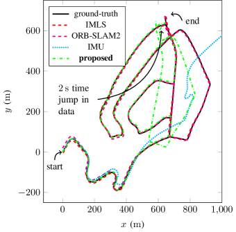
V-C Results on Sequences 00, 02 and 05
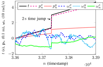
Following the procedure described in Section V-B, the proposed method seems to have degraded performances on seq. 00, 02 and 05, see e.g. Figure 9. However, the behavior is wholly explainable: data are missing for a couple of seconds due to logging problems which appear both for IMU and ground-truth. This is illustrated in Figure 10 for seq. 02 where we plot available data over time. We observe jump in the IMU and ground-truth signals, that illustrate data are missing between and . The problem was corrected manually when using those sequences in the training phase described in Section V.
Although those sequences could have been discarded due to logging problems, we used them for testing without correcting their problems. This naturally results in degraded performance, but also evidences our method is remarkably robust to such problems in spite of their inherent harmfulness. For instance, the time jump of seq. 02 results in estimate shift, but no divergence occurs for all that, see Figure 9.

V-D Discussion
The performances are owed to three components: ) the use of a recent IEKF that has been proved to be well suited for IMU based localization; ) incorporation of side information in the form of pseudo-measurements with dynamic noise parameter adaptation learned by a neural network; and ) accounting for a “loose” misalignment between the IMU frame and the car frame.
As concerns ), it should be stressed the method is perfectly suited to the use of a conventional EKF and is easily adapted if need be. However we advocate the use of an IEKF owing to its accuracy and convergence properties. To illustrate the benefits of points ) and ), we consider two sub-versions of the proposed algorithm. One without alignment, i.e. where and are not included in the state and fixed at their initial values , , and a second one that uses the static filter parameters (18)-(20).
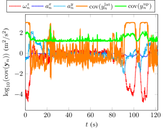
End trajectory results for the highway seq. 01 are plotted in Figure 7, where we see that the two sub-version methods have trouble when the car is turning. Therefore their respective translational errors are higher than the full version of the proposed method: the proposed method achieves 1.11%, the method without alignment level arm achieves 1.65%, and the absence of covariance adaptation yields 1.94% error. All methods have the same rotational error . This could be anticipated for the considered sequence since the full method has the same rotational error than standard IMU integration method.
As systems with equipped AI-based approaches may be hard to certify for commercial or industrial use [41], we note adaptation rules may be inferred from the AI-based adapter, and encoded in an EKF using pseudo-measurements. To this aim, we plot the covariances computed by the adapter for seq. 01 in Figure 8. The adapter clearly increases the covariances during the bend, i.e. when the gyro yaw rate is important. This is especially the case for the zero velocity measurement (15): its associated covariance is inflated by a factor of between and . This illustrates the kind of information the adapter has learned. Interestingly, we see large discrepancies may occur between the actual statistical uncertainty (which should clearly be below ) and the inflated covariances whose values are computed for the sole purpose of filter’s performance enhancement. Indeed, such a large noise parameter inflation indicates the AI-based part of the algorithm has learned and recognizes that pseudo-measurements have no value for localization at those precise moments, so the filter should barely consider them.
VI Conclusion
This paper proposes a novel approach for inertial dead-reckoning for wheeled vehicles. Our approach exploits deep neural networks to dynamically adapt the covariance of simple assumptions about the vehicle motions which are leveraged in an invariant extended Kalman filter that performs localization, velocity and sensor bias estimation. The entire algorithm is fed with IMU signals only, and requires no other sensor. The method leads to surprisingly accurate results, and opens new perspectives. In future work, we would like to address the learning of the Kalman covariance matrices for images, and also the issue of generalization from one vehicle to another.
Acknowledgments
The authors would like to thank J-E. Deschaud for sharing the results of the IMLS algorithm [6], and Paul Chauchat for relevant discussions.
| test seq. | environment | IMLS [6] | ORB-SLAM2 [7] | IMU | proposed | ||||||
|---|---|---|---|---|---|---|---|---|---|---|---|
| length | duration | ||||||||||
| () | () | (%) | () | (%) | () | (%) | () | (%) | () | ||
| 00 | 3.7 | 454 | urban | 1.46 | 0.17 | 1.33 | 0.29 | 426 | 4.68 | 7.40 | 2.65 |
| 02 | 5.1 | 466 | urban | 2.42 | 0.12 | 1.84 | 0.28 | 346 | 0.87 | 2.85 | 0.38 |
| 05 | 2.2 | 278 | urban | 0.83 | 0.10 | 0.75 | 0.22 | 189 | 0.52 | 2.76 | 0.86 |
References
- [1] G. Bresson, Z. Alsayed, L. Yu et al., “Simultaneous Localization and Mapping: A Survey of Current Trends in Autonomous Driving,” IEEE Transactions on Intelligent Vehicles, vol. 2, no. 3, pp. 194–220, 2017.
- [2] OxTS, “Why it is Necessary to Integrate an Inertial Measurement Unit with Imaging Systems on an Autonomous Vehicle,” https : / / www . oxts . com / technical-notes/why-use-ins-with-autonomous-vehicle/, 2018.
- [3] A. Geiger, P. Lenz, C. Stiller et al., “Vision meets robotics: The KITTI dataset,” The International Journal of Robotics Research, vol. 32, no. 11, pp. 1231–1237, 2013.
- [4] A. Barrau and S. Bonnabel, “The Invariant Extended Kalman Filter as a Stable Observer,” IEEE Transactions on Automatic Control, vol. 62, no. 4, pp. 1797–1812, 2017.
- [5] ——, “Invariant Kalman Filtering,” Annual Review of Control, Robotics, and Autonomous Systems, vol. 1, no. 1, pp. 237–257, 2018.
- [6] J.-E. Deschaud, “IMLS-SLAM: Scan-to-Model Matching Based on 3D Data,” in International Conference on Robotics and Automation. IEEE, 2018.
- [7] R. Mur-Artal and J. Tardos, “ORB-SLAM2: An Open-Source SLAM System for Monocular, Stereo, and RGB-D Cameras,” Transactions on Robotics, vol. 33, no. 5, pp. 1255–1262, 2017.
- [8] F. Tschopp, T. Schneider, A. W. Palmer et al., “Experimental Comparison of Visual-Aided Odometry Methods for Rail Vehicles,” IEEE Robotics and Automation Letters, vol. 4, no. 2, pp. 1815–1822, 2019.
- [9] M. Mousa, K. Sharma, and C. G. Claudel, “Inertial Measurement Units-Based Probe Vehicles: Automatic Calibration, Trajectory Estimation, and Context Detection,” IEEE Transactions on Intelligent Transportation Systems, vol. 19, no. 10, pp. 3133–3143, 2018.
- [10] J. Wahlstrom, I. Skog, J. G. P. Rodrigues et al., “Map-Aided Dead-Reckoning Using Only Measurements of Speed,” IEEE Transactions on Intelligent Vehicles, vol. 1, no. 3, pp. 244–253, 2016.
- [11] A. Mahmoud, A. Noureldin, and H. S. Hassanein, “Integrated Positioning for Connected Vehicles,” IEEE Transactions on Intelligent Transportation Systems, pp. 1–13, 2019.
- [12] R. Karlsson and F. Gustafsson, “The Future of Automotive Localization Algorithms: Available, reliable, and scalable localization: Anywhere and anytime,” IEEE Signal Processing Magazine, vol. 34, no. 2, pp. 60–69, 2017.
- [13] K. Wu, C. Guo, G. Georgiou et al., “VINS on Wheels,” in International Conference on Robotics and Automation. IEEE, 2017, pp. 5155–5162.
- [14] A. Brunker, T. Wohlgemuth, M. Frey et al., “Odometry 2.0: A Slip-Adaptive EIF-Based Four-Wheel-Odometry Model for Parking,” IEEE Transactions on Intelligent Vehicles, vol. 4, no. 1, pp. 114–126, 2019.
- [15] F. Zheng and Y.-H. Liu, “SE(2)-Constrained Visual Inertial Fusion for Ground Vehicles,” IEEE Sensors Journal, vol. 18, no. 23, pp. 9699–9707, 2018.
- [16] M. Buczko, V. Willert, J. Schwehr et al., “Self-Validation for Automotive Visual Odometry,” in Intelligent Vehicles Symposium. IEEE, 2018, pp. 1–6.
- [17] M. Kok, J. D. Hol, and T. B. Schön, “Using Inertial Sensors for Position and Orientation Estimation,” Foundations and Trends® in Signal Processing, vol. 11, no. 1-2, pp. 1–153, 2017.
- [18] A. Ramanandan, A. Chen, and J. Farrell, “Inertial Navigation Aiding by Stationary Updates,” IEEE Transactions on Intelligent Transportation Systems, vol. 13, no. 1, pp. 235–248, 2012.
- [19] G. Dissanayake, S. Sukkarieh, E. Nebot et al., “The Aiding of a Low-cost Strapdown Inertial Measurement Unit Using Vehicle Model Constraints for Land Vehicle Applications,” IEEE Transactions on Robotics and Automation, vol. 17, no. 5, pp. 731–747, 2001.
- [20] M. Brossard, A. Barrau, and S. Bonnabel, “RINS-W: Robust Inertial Navigation System on Wheels,” Submitted to IROS 2019, 2019. [Online]. Available: https://hal.archives-ouvertes.fr/hal-02057117/file/main.pdf
- [21] F. Aghili and C.-Y. Su, “Robust Relative Navigation by Integration of ICP and Adaptive Kalman Filter Using Laser Scanner and IMU,” IEEE/ASME Transactions on Mechatronics, vol. 21, no. 4, pp. 2015–2026, 2016.
- [22] H. Yan, Q. Shan, and Y. Furukawa, “RIDI: Robust IMU Double Integration,” in European Conference on Computer Vision, 2018.
- [23] C. Chen, X. Lu, A. Markham et al., “IONet: Learning to Cure the Curse of Drift in Inertial Odometry,” in Conference on Artificial Intelligence AAAI, 2018.
- [24] T. Haarnoja, A. Ajay, S. Levine et al., “Backprop KF: Learning Discriminative Deterministic State Estimators,” in Advances in Neural Information Processing Systems, 2016.
- [25] K. Liu, K. Ok, W. Vega-Brown et al., “Deep Inference for Covariance Estimation: Learning Gaussian Noise Models for State Estimation,” in International Conference on Robotics and Automation. IEEE, 2018.
- [26] M. Brossard and S. Bonnabel, “Learning Wheel Odometry and IMU Errors for Localization,” in International Conference on Robotics and Automation. IEEE, 2019.
- [27] F. Castella, “An Adaptive Two-Dimensional Kalman Tracking Filter,” IEEE Transactions on Aerospace and Electronic Systems, vol. AES-16, no. 6, pp. 822–829, 1980.
- [28] P. Abbeel, A. Coates, M. Montemerlo et al., “Discriminative Training of Kalman Filters,” in Robotics: Science and Systems, vol. 2, 2005.
- [29] M. Tahk and J. Speyer, “Target tracking problems subject to kine-matic constraints,” IEEE Transactions on Automatic Control, vol. 32, no. 2, pp. 324–326, 1990.
- [30] D. Simon, “Kalman Filtering with State Constraints: A Survey of Linear and Nonlinear Algorithms,” IET Control Theory & Applications, vol. 4, no. 8, pp. 1303–1318, 2010.
- [31] A. Barrau and S. Bonnabel, “Aligment Method for an Inertial Unit,” Patent 15/037,653, 2016.
- [32] M. Brossard, S. Bonnabel, and A. Barrau, “Unscented Kalman Filter on Lie Groups for Visual Inertial Odometry,” in International Conference on Intelligent Robots and Systems. IEEE/RSJ, 2018.
- [33] S. Heo and C. G. Park, “Consistent EKF-Based Visual-Inertial Odometry on Matrix Lie Group,” IEEE Sensors Journal, vol. 18, no. 9, pp. 3780–3788, 2018.
- [34] R. Hartley, M. G. Jadidi, J. W. Grizzle et al., “Contact-Aided Invariant Extended Kalman Filtering for Legged Robot State Estimation,” in Robotics Science and Systems, 2018.
- [35] I. Goodfellow, Y. Bengio, and A. Courville, Deep Learning. The MIT press, 2016.
- [36] D. P. Kingma and J. Ba, “ADAM: A Method for Stochastic Optimization,” in International Conference on Learning Representations, 2014.
- [37] G. Parisi, R. Kemker, J. Part et al., “Continual Lifelong Learning with Neural Networks: A Review,” Neural Networks, vol. 113, pp. 54–71, 2019.
- [38] T. Qin, J. Pan, S. Cao et al., “A General Optimization-based Framework for Local Odometry Estimation with Multiple Sensors,” 2019.
- [39] M. Ramezani and K. Khoshelham, “Vehicle Positioning in GNSS-Deprived Urban Areas by Stereo Visual-Inertial Odometry,” IEEE Transactions on Intelligent Vehicles, vol. 3, no. 2, pp. 208–217, 2018.
- [40] S. Heo, J. Cha, and C. G. Park, “EKF-Based Visual Inertial Navigation Using Sliding Window Nonlinear Optimization,” IEEE Transactions on Intelligent Transportation Systems, pp. 1–10, 2018.
- [41] N. Sünderhauf, O. Brock, W. Scheirer et al., “The limits and potentials of deep learning for robotics,” The International Journal of Robotics Research, vol. 37, no. 4-5, pp. 405–420, 2018.
Appendix A
The Invariant Extended Kalman Filter (IEKF) [4, 5] is an EKF based on an alternative state error. One must define a linearized error, an underlying group to derive the exponential map, and then methodology is akin to the EKF’s.
A-1 Linearized Error
the filter state is given by (8). The state evolution is given by the dynamics (5)-(7) and (12)-(13), see Section II. Along the lines of [4], variables are embedded in the Lie group (see Appendix B for the definition of and its exponential map). Then biases vector is merely treated as a vector, that is, as an element of viewed as a Lie group endowed with standard addition, is treated as element of Lie group , and as a vector. Once the state is broken into several Lie groups, the linearized error writes as the concatenation of corresponding linearized errors, that is,
| (21) |
where state uncertainty is a zero-mean Gaussian variable with covariance . As (15) are measurements expressed in the robot’s frame, they lend themselves to the Right IEKF methodology. This means each linearized error is mapped to the state using the corresponding Lie group exponential map, and multiplying it on the right by elements of the state space. This yields:
| (22) | ||||
| (23) | ||||
| (24) | ||||
| (25) |
where denotes estimated state variables.
A-2 Propagation Step
we apply (5)-(7) and (12)-(13) to propagate the state and obtain and associated covariance through the Riccati equation (11) where the Jacobians , are related to the evolution of error (21) and write:
| (26) | ||||
| (27) |
with , , and denotes the classical covariance matrix of the process noise as in Section IV-B.
A-3 Update Step
the measurement vector is computed by stacking the motion information
| (28) |
with assessed uncertainty a zero-mean Gaussian variable with covariance . We then compute an updated state and updated covariance following the IEKF methodology, i.e. we compute
| (29) | ||||
| (30) | ||||
| (31) | ||||
| (32) | ||||
| (33) | ||||
| (34) | ||||
| (35) | ||||
| (36) |
summarized as Kalman gain (30), state innovation (31), state update (32)-(35) and covariance update (36), where is the measurement Jacobian matrix with respect to linearized error (21) and thus given as:
| (37) |
where selects the two first row of the right part of (37), and .
Appendix B
The Lie group is an extension of the Lie group and is described as follows, see [4] where it was first introduced. A matrix is defined as
| (40) |
The uncertainties are mapped to the Lie algebra through the transformation defined as
| (41) | ||||
| (44) |
where , and . The closed-form expression for the exponential map is given as
| (45) |
where and , and which inherently uses the exponential of , defined as
| (46) | ||||
| (47) |