Optimal Caching Designs for Perfect, Imperfect and Unknown File Popularity Distributions in Large-Scale Multi-Tier Wireless Networks

Chencheng Ye, Ying Cui, Yang Yang and Rui Wang C. Ye and Y. Cui are with Shanghai Jiao Tong University, China. Y. Yang is with University of Luxembourg, Luxembourg. R. Wang is with Southern University of Science and Technology, China.
Abstract

Most existing caching solutions for wireless networks rest on the ideal assumption that the file popularity distribution is perfectly known. In this paper, we consider optimal random caching designs for perfect, imperfect and unknown file popularity distributions in a large-scale multi-tier wireless network. First, in the case of perfect file popularity distribution, we formulate the successful transmission probability (STP) optimization problem, which is nonconvex. We propose an efficient parallel iterative algorithm to obtain a stationary point based on parallel successive convex approximation (SCA). Then, in the case of imperfect file popularity distribution, we formulate the worst-case STP maximization problem. To solve this challenging robust optimization problem, we transform it to an equivalent complementary geometric programming (CGP), and propose an efficient iterative algorithm to obtain a stationary point based on SCA. To the best of our knowledge, this is the first work explicitly considering the estimation error of file popularity distribution in the optimization of caching design. Next, in the case of unknown file popularity distribution, we formulate the stochastic STP (i.e., the STP in the stochastic form) maximization problem. This is a challenging nonconvex stochastic optimization problem, and we develop an efficient iterative algorithm to obtain a stationary point based on stochastic parallel SCA. As far as we know, this is the first work considering stochastic optimization in a large-scale wireless network. Finally, by numerical results, we show that the proposed solutions achieve notable gains over existing schemes in all three cases, and reveal the values of the robust caching optimization and stochastic caching optimization in the cases of imperfect file popularity distribution and unknown file popularity distribution, respectively.

Index Terms:
Cache, multi-tier wireless network, stochastic geometry, robust optimization, stochastic optimization, complementary geometric programming

I Introduction

The rapid proliferation of smart mobile devices has triggered an unprecedented growth of the global mobile data traffic. Caching content closer to end users, e.g., at base stations (BSs) [1, 2, 3, 4, 5, 6, 7, 8, 9, 10] or even at end users [11, 12], has been proposed as an effective way to support the dramatic traffic growth, by reducing the distance between popular contents and requesters, and alleviating the backhaul load. In addition, caching has also been jointly designed with multicast [5, 7, 10] and cooperation [1, 2]. In this paper, we focus on caching at BSs, and a large body of recent research would be out of the scope of this paper.

Caching in single-tier wireless networks has been actively studied [3, 4, 5]. Specifically, in [3], the authors consider the optimal caching design and transmission strategy to minimize the required link capacity in a square grid wireless network. In [4] and [5], the authors consider random caching at BSs, analyze and optimize the hit probability [4] and the successful transmission probability (STP) [5] in large-scale wireless networks that capture the stochastic nature of geographic locations of BSs and users.111 The stochastic network model is a widely used tractable model that allows to study the average behavior of a network using mathematical tools from stochastic geometry and is about as accurate as the standard grid model, when compared to an actual network [13]. As caching can successfully alleviate the urgent backhaul requirement for small cells, a significant amount of research effort has been devoted to optimal caching design in multi-tier wireless networks [6, 7, 8, 9, 10]. For instance, in [6], the authors consider coded and uncoded caching at small BSs to minimize the expected downloading time in a macro cell with multiple small BSs and users at fixed locations. In [7, 8, 9, 10], the authors consider hybrid caching [7] and random caching [8, 9, 10] in large-scale multi-tier wireless networks, and focus on the analysis and optimization of the STP. Specifically, in our previous work [7], we obtain optimal hybrid caching design for a two-tier wireless network. In [8] and [9], the authors obtain optimal caching design for a multi-tier network in the case of uniform signal-to-interference ratio (SIR) threshold for all users. In the general case of arbitrary SIR thresholds for users, the optimization problem is nonconvex, and in [9], an optimal caching solution of a simplified convex problem is used as a sub-optimal solution of the original nonconvex problem. In our previous work [10], a stationary point of the nonconvex problem is obtained only for a two-tier wireless network. Note that most existing works on caching [1, 2, 3, 4, 5, 6, 7, 8, 9, 10, 11, 12] assume that the file popularity distribution is perfectly known. In practice, however, such an assumption cannot be reasonably justified [14].

Some recent works consider caching design in the case that the file popularity distribution is not known and only instantaneous file requests from users can be observed[15, 16, 17, 18, 19, 20, 21, 22, 23, 24]. These works generally fall into two categories. One category adopts two-stage methods for caching design in the case of unknown file popularity distribution [15, 17, 18, 19, 16]. Specifically, in the first stage, the file popularity distribution is estimated based on historical file requests, via various learning approaches; in the second stage, caching schemes are proposed based on the estimated popularity distribution. To be specific, in [15] and [19], the file popularity distribution is estimated using transfer learning [15] and file feature space partitioning [19]. Based on the estimated file popularity distribution, the authors consider caching the most popular files, and analyze the backhaul offloading [15] and cache hit [19]. In [17], the request frequency for each file obtained from historical file requests is considered as the popularity of the file, and the performance gap for minimizing the offloading time caused by the estimation error is analyzed. In [18], the file popularity distribution is estimated by learning user preferences via probabilistic latent semantic analysis, and a greedy algorithm is proposed to obtain a caching solution of the offloading probability maximization problem (under the estimated file popularity distribution) with performance guarantee. In [16], given apriori information on the file popularity distribution, the file request rate is estimated using Bayesian framework, and an asymptotically optimal policy is proposed to maximize the hit probability (under the estimated file popularity distribution). Note that these works [15, 17, 18, 19, 16] consider either simple caching design without performance guarantee, such as caching the most popular files at each BS [15, 19], or optimization-based caching design obtained by optimizing simple performance metrics that may not fully reflect natures of wireless networks (such as fading [17] and stochastic locations of BSs and users [18, 16]). In addition, note that [15, 17, 18, 19, 16] fail to consider estimation errors in designing caching schemes.

The other category adopts single-stage methods for caching design [20, 21, 22, 23, 24] in the case of unknown file popularity, where caching solutions are gradually updated while accumulating file requests using stochastic optimization [20] or reinforcement learning [21, 22, 23, 24]. Compared with two-stage methods, the caching solutions obtained by single stage methods can be continuously improved as new file requests are observed. Specifically, in [20], the authors optimize power control and caching for video streaming in a multi-cell multi-user MIMO network using techniques for stochastic optimization. In [21] and [22], the authors formulate the optimal caching design problem for a single-cell wireless network [21] and the optimal cooperative caching design problem for a multi-cell wireless network [22], and develop low-complexity algorithms to obtain approximate solutions using results for multi-armed bandit problems. In [23] and [24], the authors formulate the dynamic optimal caching design problem for a single-cell wireless network [23] and a multi-cell wireless network [24], and develop approximate solutions using Q-learning techniques. However, the fixed network topologies considered in [20, 21, 22, 24, 23] cannot fully capture the geographic features of the locationsof BS and users. In addition, the caching solutions in [20, 21, 22, 24, 23] are for one BS [21, 23] or a single-tier of BSs [20, 22, 24].

Therefore, further studies are needed to optimize caching design in multi-tier wireless networks when perfect file popularity distribution is not known. In this paper, we consider optimal random caching design in three cases, i.e., the case of perfect file popularity distribution (where the file popularity distribution has been estimated, and the estimation error is negligible), the case of imperfect file popularity distribution (where the file popularity distribution has been estimated, and a deterministic bound of the estimation error is known) and the case of unknown file popularity distribution (where there is no prior information of the file popularity distribution, but instantaneous file requests from some users can be observed over time), in a large-scale multi-tier wireless network. Our main contributions are summarized below.

  • In the case of perfect file popularity distribution, we formulate the STP maximization problem, which is nonconvex with a complicated objective function. We propose an efficient parallel iterative algorithm to obtain a stationary point based on parallel successive convex approximation (SCA) [25]. Specifically, by carefully designing an approximation function for each tier, we obtain closed-form optimal solutions for the approximate functions of all tiers at each iteration, and hence can significantly reduce the computational complexity and improve the convergence speed of the iterative algorithm.

  • In the case of imperfect file popularity distribution, we formulate the worst-case STP (over all possible values of the true file popularity distribution) maximization problem. This is a challenging robust optimization problem which does not lie in the category of convex-concave games that can be easily solved. We transform it to an equivalent complementary geometric programming (CGP) and propose an efficient iterative algorithm to obtain a stationary point using SCA [26]. Note that this case corresponds to that considered in the second stage of the two-stage methods proposed in [15, 17, 18, 19, 16]. But the essential difference is that we explicitly consider the estimation error of file popularity distribution in the optimization of caching design.

  • In the case of unknown file popularity distribution, we formulate the stochastic STP (i.e., the STP in the stochastic form) maximization problem. This is a challenging nonconvex stochastic optimization problem, and we develop an efficient parallel iterative algorithm to obtain a stationary point based on stochastic parallel SCA [27]. Specifically, by carefully designing an approximation function for each tier, we obtain closed-form optimal solutions for the approximate functions of all tiers at each iteration, make full use of instantaneous file requests from users at each slot, and significantly improve the convergence speed of the iterative algorithm. Note that this case corresponds to that considered in the single-stage methods proposed in [20, 21, 22, 23, 24]. The key difference is that we consider stochastic optimization in a large-scale wireless network which captures the channel fading, interference and stochastic nature of wireless networks.

  • Finally, by numerical simulations, we show the convergence of the proposed solutions. We also show that the proposed solutions achieve notable gains over existing schemes in all three cases.

II System Model

II-A Network Model

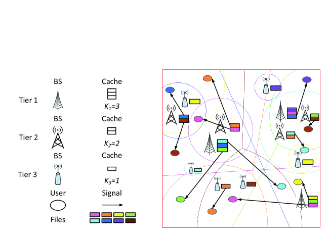
In this part, we first elaborate on the network model which extends those in [8, 9, 10] in the sense that besides perfect file popularity distribution, it also models imperfect and unknown file popularity distributions. We consider a large-scale M𝑀M-tier network consisting of M𝑀M tiers of BSs, where M2𝑀2M\geq 2,222Note that for M=1𝑀1M=1, the case of perfect file popularity distribution has been studied in our previous work [5], and the cases of imperfect and unknown file popularity distributions can be easily investigated following the results for M2𝑀2M\geq 2 in this paper. as shown in Fig. 1. The locations of the BSs in tier m𝑚m are spatially distributed as an independent homogeneous Poisson point process (PPP), denoted as ΦmsubscriptΦ𝑚\Phi_{m}, with density λmsubscript𝜆𝑚\lambda_{m}, for all m{1,2,,M}𝑚12𝑀m\in\mathcal{M}\triangleq\{1,2,\dots,M\}. The locations of the users are also distributed as an independent homogeneous PPP ΦusubscriptΦ𝑢\Phi_{u}. Consider a discrete-time system with time being slotted. Let t{1,2,}𝑡12t\in\{1,2,\dots\} denote the slot index. Each BS in tier m𝑚m has one transmit antenna with fixed transmission power Pmsubscript𝑃𝑚P_{m}. Each user has one receive antenna. All BSs are operating on the same frequency band and each BS adopts an orthogonal transmission mechanism over frequency or time at each slot. Both path loss and small-scale fading are considered: for path loss, a transmitted signal from either tier with distance D𝐷D is attenuated by a factor Dαsuperscript𝐷𝛼D^{-\alpha}, where α>2𝛼2\alpha>2 is the path loss exponent [7, 8, 9, 10]; for small-scale fading, at each slot, Rayleigh fading channels are adopted. Since a multi-tier network is primarily interference-limited, we ignore the thermal noise for simplicity[9].

Let 𝒩{1,2,,N}𝒩12𝑁\mathcal{N}\triangleq\{1,2,\cdots,N\} denote the set of N𝑁N files in the M𝑀M-tier network. For ease of illustration, as in [6, 7, 8, 9, 10, 15], assume that all files have the same size.333The results in this paper can be easily extended to the case of different file sizes by considering file combinations of the same total size, but formed by files of possibly different sizes [10]. At each slot, a user requests at most one file at random. Let πs(t){0}𝒩subscript𝜋𝑠𝑡0𝒩\pi_{s}(t)\in\{0\}\cup\mathcal{N} denote the file request status of user sΦu𝑠subscriptΦ𝑢s\in\Phi_{u} at slot t{1,2,}𝑡12t\in\{1,2,\dots\}, where πs(t)=0subscript𝜋𝑠𝑡0\pi_{s}(t)=0 if user s𝑠s does not request any file and πs(t)=n𝒩subscript𝜋𝑠𝑡𝑛𝒩\pi_{s}(t)=n\in\mathcal{N} if user s𝑠s requests file n𝑛n. For ease of analysis, assume πs(t)subscript𝜋𝑠𝑡\pi_{s}(t), sΦu𝑠subscriptΦ𝑢s\in\Phi_{u}, t{1,2,}𝑡12t\in\{1,2,\dots\} are i.i.d. with respect to s𝑠s and t𝑡t [7, 8, 9, 10, 15].444 The results in this paper can be extended to the case where there are multiple classes of users and file requests of users in the same class are i.i.d.. Denoted anPr[πs(t)=n|πs(t)0][0,1]subscript𝑎𝑛Prdelimited-[]subscript𝜋𝑠𝑡conditional𝑛subscript𝜋𝑠𝑡001a_{n}\triangleq{\rm Pr}[\pi_{s}(t)=n|\pi_{s}(t)\neq 0]\in[0,1], sΦu𝑠subscriptΦ𝑢s\in\Phi_{u}, n𝒩𝑛𝒩n\in\mathcal{N}, where n𝒩an=1subscript𝑛𝒩subscript𝑎𝑛1\sum_{n\in\mathcal{N}}a_{n}=1. Thus, 𝐚(an)n𝒩𝐚subscriptsubscript𝑎𝑛𝑛𝒩\mathbf{a}\triangleq(a_{n})_{n\in\mathcal{N}} represents the file popularity distribution, which usually evolves at a slower timescale. In this paper, we consider the following three cases of file popularity distribution.
Perfect file popularity distribution: In this case, we assume that the file popularity distribution has been estimated by some learning methods, and the estimation error is negligible. That is, the exact value of 𝐚𝐚\mathbf{a} is known.
Imperfect file popularity distribution: In this case, we assume that the file popularity distribution has been estimated by some learning methods, and a deterministic bound of the estimation error is known. Note that this case corresponds to that considered in the second stage of the two-stage methods proposed in [15, 17, 18]. Let 𝐚^(a^n)n𝒩^𝐚subscriptsubscript^𝑎𝑛𝑛𝒩\widehat{\mathbf{a}}\triangleq(\widehat{a}_{n})_{n\in\mathcal{N}} denote the estimated file popularity distribution, and let 𝚫(Δn)n𝒩𝚫subscriptsubscriptΔ𝑛𝑛𝒩\boldsymbol{\Delta}\triangleq(\Delta_{n})_{n\in\mathcal{N}} denote the estimation error. Assume n𝒩a^n=1subscript𝑛𝒩subscript^𝑎𝑛1\sum_{n\in\mathcal{N}}\widehat{a}_{n}=1, n𝒩Δn=0subscript𝑛𝒩subscriptΔ𝑛0\sum_{n\in\mathcal{N}}\Delta_{n}=0, and |Δn|εnsubscriptΔ𝑛subscript𝜀𝑛|\Delta_{n}|\leq\varepsilon_{n} for some known εn>0subscript𝜀𝑛0\varepsilon_{n}>0, for all n𝒩𝑛𝒩n\in\mathcal{N}, which are usually satisfied for effective learning methods. The (true) file popularity distribution is given by 𝐚=𝐚^+𝚫𝐚^𝐚𝚫\mathbf{a}=\widehat{\mathbf{a}}+\boldsymbol{\Delta}, and satisfies 𝐚𝒜{(xn)n𝒩|a¯nxna¯n,n𝒩,n𝒩xn=1}𝐚𝒜conditional-setsubscriptsubscript𝑥𝑛𝑛𝒩formulae-sequencesubscript¯𝑎𝑛subscript𝑥𝑛subscript¯𝑎𝑛formulae-sequence𝑛𝒩subscript𝑛𝒩subscript𝑥𝑛1\mathbf{a}\in\mathcal{A}\triangleq\left\{(x_{n})_{n\in\mathcal{N}}\ \middle|\ \underline{a}_{n}\leq x_{n}\leq\overline{a}_{n},n\in\mathcal{N},\sum_{n\in\mathcal{N}}x_{n}=1\right\}, where a¯nmax{a^nεn,0}subscript¯𝑎𝑛subscript^𝑎𝑛subscript𝜀𝑛0\underline{a}_{n}\triangleq\max\{\widehat{a}_{n}-\varepsilon_{n},0\}, and a¯nmin{a^n+εn,1}subscript¯𝑎𝑛subscript^𝑎𝑛subscript𝜀𝑛1\overline{a}_{n}\triangleq\min\{\widehat{a}_{n}+\varepsilon_{n},1\} for all n𝒩𝑛𝒩n\in\mathcal{N}.
Unknown file popularity distribution: In this case, we assume that there is no prior information of the file popularity distribution 𝐚𝐚\mathbf{a}, but the file requests from the users in some set 𝒰Φu𝒰subscriptΦ𝑢\mathcal{U}\subseteq\Phi_{u} without bias can be observed over time. Here 𝒰𝒰\mathcal{U} can represent the set of users located in the physical area of a BS or a cluster of BSs.555 For example, a user can submit its file request to its nearest BS, and each BS can gather file requests corresponding to an unbiased observation of the file popularity distribution. Note that this case corresponds to that considered in the single-stage methods proposed in [20, 21, 22, 23, 24].

The M𝑀M-tier network consists of cache-enabled BSs. In tier m𝑚m, each BS is equipped with a cache of size Km<Nsubscript𝐾𝑚𝑁K_{m}<N (in number of files) to store Kmsubscript𝐾𝑚K_{m} different popular files out of N𝑁N. We say every Kmsubscript𝐾𝑚K_{m} different files form a combination. Thus, there are in total (NKm)binomial𝑁subscript𝐾𝑚\binom{N}{K_{m}} different combinations, each with Kmsubscript𝐾𝑚K_{m} different files. Let msubscript𝑚\mathcal{I}_{m} denote the set of indices for the (NKm)binomial𝑁subscript𝐾𝑚\binom{N}{K_{m}} combinations. More detailed descriptions of msubscript𝑚\mathcal{I}_{m} and m,nsubscript𝑚𝑛\mathcal{I}_{m,n} can be found in [5, 7, 10].

Refer to caption
Figure 1: Network model. M=3𝑀3M=3 and N=8𝑁8N=8. Each file n𝒩𝑛𝒩n\in\mathcal{N} corresponds to a Voronoi tessellation (in the same color as the file), determined by the locations and transmission powers of all BSs storing this file.

II-B Caching and User Association

To provide high spatial file diversity, we consider random caching in the cache-enabled M𝑀M-tier network [8, 9, 10], as illustrated in Fig. 1. In particular, each BS in tier m𝑚m stores Kmsubscript𝐾𝑚K_{m} different files with certain probability [8, 9, 10]. The probability that combination im𝑖subscript𝑚i\in\mathcal{I}_{m} is stored at each BS in tier m𝑚m is pm,isubscript𝑝𝑚𝑖p_{m,i}, where pm,isubscript𝑝𝑚𝑖p_{m,i} satisfies:

0pm,i1,m,im,formulae-sequence0subscript𝑝𝑚𝑖1formulae-sequence𝑚𝑖subscript𝑚\displaystyle 0\leq p_{m,i}\leq 1,\ m\in\mathcal{M},\quad i\in\mathcal{I}_{m}, (1)
impm,i=1,m.formulae-sequencesubscript𝑖subscript𝑚subscript𝑝𝑚𝑖1𝑚\displaystyle\sum_{i\in\mathcal{I}_{m}}p_{m,i}=1,\quad m\in\mathcal{M}. (2)

A random caching design is specified by the caching distributions for file combinations 𝐩(pm,i)m,im𝐩subscriptsubscript𝑝𝑚𝑖formulae-sequence𝑚𝑖subscript𝑚\mathbf{p}\triangleq(p_{m,i})_{m\in\mathcal{M},i\in\mathcal{I}_{m}}. Let m,nmsubscript𝑚𝑛subscript𝑚\mathcal{I}_{m,n}\subset\mathcal{I}_{m} denote the set of indices for the (N1Km1)binomial𝑁1subscript𝐾𝑚1\binom{N-1}{K_{m}-1} combinations containing file n𝑛n. Based on 𝐩𝐩\mathbf{p}, we also define the probability that file n𝑛n is stored at a BS in tier m𝑚m, i.e.,

Tm,nim,npm,i,m,n𝒩.formulae-sequencesubscript𝑇𝑚𝑛subscript𝑖subscript𝑚𝑛subscript𝑝𝑚𝑖formulae-sequence𝑚𝑛𝒩\displaystyle T_{m,n}\triangleq\sum_{i\in\mathcal{I}_{m,n}}p_{m,i},\quad m\in\mathcal{M},\ n\in\mathcal{N}. (3)

From [4, 5, 7, 10], we know that the constraints on 𝐩𝐩\mathbf{p} in (1), (2) and (3) can be equivalently rewritten as the following constraints on 𝐓(Tm,n)m,n𝒩𝐓subscriptsubscript𝑇𝑚𝑛formulae-sequence𝑚𝑛𝒩\mathbf{T}\triangleq(T_{m,n})_{m\in\mathcal{M},n\in\mathcal{N}}:

0Tm,n1,m,n𝒩,formulae-sequence0subscript𝑇𝑚𝑛1formulae-sequence𝑚𝑛𝒩\displaystyle 0\leq T_{m,n}\leq 1,\quad m\in\mathcal{M},\ n\in\mathcal{N}, (4)
n𝒩Tm,n=Km,m.formulae-sequencesubscript𝑛𝒩subscript𝑇𝑚𝑛subscript𝐾𝑚𝑚\displaystyle\sum\limits_{n\in\mathcal{N}}T_{m,n}=K_{m},\quad m\in\mathcal{M}. (5)

The constraints in (5) are due to the fact that each file combination in tier m𝑚m contains Kmsubscript𝐾𝑚K_{m} different files and the sum of the caching probabilities for all file combinations is one. The details can be found in [5]. For any 𝐓𝐓\mathbf{T} satisfying (4) and (5), one corresponding 𝐩𝐩\mathbf{p} satisfying (1), (2) and (3) can be easily obtained using the method proposed in [4].666When the file popularity changes, the cache content of each BS can be easily updated based on its previous cached content. Random caching design is specified by the caching distributions for file combinations 𝐩𝐩\mathbf{p}, the size of which is m=1M(NKm)superscriptsubscript𝑚1𝑀binomial𝑁subscript𝐾𝑚\sum_{m=1}^{M}\binom{N}{K_{m}}. However, later we shall see that the performance metrics and optimal random caching design problems considered in this paper depend only on the caching probabilities for files 𝐓𝐓\mathbf{T}, the size of which is MN𝑀𝑁MN.

If a file is stored in a tier, a user requesting the file is associated with the BS which provides the maximum long-term average received power among all BSs storing the file [8, 9, 10]. Otherwise, the user will be served through other service mechanisms [8, 9, 10], the investigation of which is beyond the scope of this paper.777 As in [8, 9, 10], we assume that user association can be done through some signaling mechanisms. For example, a user can submit its file request to its nearest BS and associates with its serving BS via the help of its nearest BS. The probability that an arbitrary user requesting file n𝑛n is associated with tier m𝑚m is given by [8, 9, 10]:

Am,n(𝐓)=λmTm,nλmTm,n+l\{m}λlTl,n(PlPm)2α,m,n𝒩.formulae-sequencesubscript𝐴𝑚𝑛𝐓subscript𝜆𝑚subscript𝑇𝑚𝑛subscript𝜆𝑚subscript𝑇𝑚𝑛subscript𝑙\𝑚subscript𝜆𝑙subscript𝑇𝑙𝑛superscriptsubscript𝑃𝑙subscript𝑃𝑚2𝛼formulae-sequence𝑚𝑛𝒩\displaystyle A_{m,n}(\mathbf{T})=\frac{\lambda_{m}T_{m,n}}{\lambda_{m}T_{m,n}+\sum_{l\in\mathcal{M}\backslash\{m\}}\lambda_{l}T_{l,n}\left(\frac{P_{l}}{P_{m}}\right)^{\frac{2}{\alpha}}},\quad m\in\mathcal{M},n\in\mathcal{N}. (6)

II-C Performance Metrics

In this paper, we study w.l.o.g. the performance of a typical user u0subscript𝑢0u_{0}, which is located at the origin. Suppose u0subscript𝑢0u_{0} requests file n𝑛n and is associated with tier m𝑚m. Let 0Φmsubscript0subscriptΦ𝑚\ell_{0}\in\Phi_{m} denote the index of the serving BS of u0subscript𝑢0u_{0}. We denote Dm,,0subscript𝐷superscript𝑚0D_{m^{\prime},\ell,0} and hm,,0d𝒞𝒩(0,1)superscriptsimilar-to𝑑subscriptsuperscript𝑚0𝒞𝒩01h_{m^{\prime},\ell,0}\stackrel{{\scriptstyle d}}{{\sim}}\mathcal{CN}\left(0,1\right) as the distance and the small-scale channel between BS ΦmsubscriptΦsuperscript𝑚\ell\in\Phi_{m^{\prime}} and u0subscript𝑢0u_{0}, respectively. For analytical tractability, as in [9, 10], we assume all BSs are active for serving their own users.888This assumption corresponds to the worst-case interference strength for the typical user. The performance obtained under this assumption provides a lower bound on the performance of the practical network where some void BSs may be shut down. In this case, the SIR of u0subscript𝑢0u_{0}, denoted by SIRm,n,0subscriptSIR𝑚𝑛0{\rm SIR}_{m,n,0}, is given by [10]:

SIRm,n,0=Dm,0,0α|hm,0,0|2Φm\{0}Dm,,0α|hm,,0|2+j\{m}ΦjDj,,0α|hj,,0|2PjPm.subscriptSIR𝑚𝑛0superscriptsubscript𝐷𝑚subscript00𝛼superscriptsubscript𝑚subscript002subscript\subscriptΦ𝑚subscript0superscriptsubscript𝐷𝑚0𝛼superscriptsubscript𝑚02subscript𝑗\𝑚subscriptsubscriptΦ𝑗superscriptsubscript𝐷𝑗0𝛼superscriptsubscript𝑗02subscript𝑃𝑗subscript𝑃𝑚\displaystyle{\rm SIR}_{m,n,0}=\frac{{D_{m,\ell_{0},0}^{-\alpha}}\left|h_{m,\ell_{0},0}\right|^{2}}{\sum\limits_{\ell\in\Phi_{m}\backslash\{\ell_{0}\}}D_{m,\ell,0}^{-\alpha}\left|h_{m,\ell,0}\right|^{2}+\sum\limits_{j\in\mathcal{M}\backslash\{m\}}\sum\limits_{\ell\in\Phi_{j}}D_{j,\ell,0}^{-\alpha}\left|h_{j,\ell,0}\right|^{2}\frac{P_{j}}{P_{m}}}. (7)

Note that the distribution of SIRm,n,0subscriptSIR𝑚𝑛0{\rm SIR}_{m,n,0} is affected by 𝐓𝐓\mathbf{T}.

We assume that file n𝑛n delivered from tier m𝑚m can be decoded correctly at u0subscript𝑢0u_{0} if SIRm,n,0τmsubscriptSIRmn0subscript𝜏m{\rm SIR_{m,n,0}\geq\tau_{m}}, where τmsubscript𝜏𝑚\tau_{m} represents a threshold for tier m𝑚m [9]. Requesters are mostly concerned about whether their desired files can be successfully received. In the following, we introduce the performance metrics in the three cases of file popularity distribution.
Perfect file popularity distribution: When the exact value of 𝐚𝐚\mathbf{a} is known, we adopt the probability that a randomly requested file by u0subscript𝑢0u_{0} is successfully transmitted, called the STP [10]:

q(𝐚,𝐓)𝑞𝐚𝐓absent\displaystyle q\left(\mathbf{a},\mathbf{T}\right)\triangleq mn𝒩anAm,n(𝐓)Pr[SIRm,n,0τm]subscript𝑚subscript𝑛𝒩subscript𝑎𝑛subscript𝐴𝑚𝑛𝐓Prdelimited-[]subscriptSIR𝑚𝑛0subscript𝜏𝑚\displaystyle\sum_{m\in\mathcal{M}}\sum_{n\in\mathcal{N}}a_{n}A_{m,n}\left(\mathbf{T}\right){\rm Pr}\left[{\rm SIR}_{m,n,0}\geq\tau_{m}\right]
=\displaystyle= mn𝒩anTm,nlθl,mTl,n+ηm,subscript𝑚subscript𝑛𝒩subscript𝑎𝑛subscript𝑇𝑚𝑛subscript𝑙subscript𝜃𝑙𝑚subscript𝑇𝑙𝑛subscript𝜂𝑚\displaystyle\sum_{m\in\mathcal{M}}\sum_{n\in\mathcal{N}}{\frac{a_{n}T_{m,n}}{\sum_{l\in\mathcal{M}}{\theta_{l,m}T_{l,n}}+\eta_{m}}}, (8)

as the performance metric,999 Note that the STP with fixed STR thresholds can be interpreted as the STP under multicast at the high user density region [5, 7, 10], and is a widely used performance metric in wireless caching [5, 7, 8, 9, 10], as it is tractable and is also closely related to some other important performance metrics, such as average transmission rate and average transmission delay. where θl,msubscript𝜃𝑙𝑚\theta_{l,m} and ηmsubscript𝜂𝑚\eta_{m} are given by:

θl,m=2λlαλm(PlPmτm)2α(B(2α,12α,11+τm)B(2α,12α))+λlλm(PlPm)2α,subscript𝜃𝑙𝑚2subscript𝜆𝑙𝛼subscript𝜆𝑚superscriptsubscript𝑃𝑙subscript𝑃𝑚subscript𝜏𝑚2𝛼superscript𝐵2𝛼12𝛼11subscript𝜏𝑚𝐵2𝛼12𝛼subscript𝜆𝑙subscript𝜆𝑚superscriptsubscript𝑃𝑙subscript𝑃𝑚2𝛼\displaystyle\theta_{l,m}=\frac{2\lambda_{l}}{\alpha\lambda_{m}}\left(\frac{P_{l}}{P_{m}}\tau_{m}\right)^{\frac{2}{\alpha}}\left(B^{\prime}\left(\frac{2}{\alpha},1-\frac{2}{\alpha},\frac{1}{1+\tau_{m}}\right)-B\left(\frac{2}{\alpha},1-\frac{2}{\alpha}\right)\right)+\frac{\lambda_{l}}{\lambda_{m}}\left(\frac{P_{l}}{P_{m}}\right)^{\frac{2}{\alpha}}, (9)
ηm=l2λlαλm(PlPmτm)2αB(2α,12α),subscript𝜂𝑚subscript𝑙2subscript𝜆𝑙𝛼subscript𝜆𝑚superscriptsubscript𝑃𝑙subscript𝑃𝑚subscript𝜏𝑚2𝛼𝐵2𝛼12𝛼\eta_{m}=\sum_{l\in\mathcal{M}}\frac{2\lambda_{l}}{\alpha\lambda_{m}}\left(\frac{P_{l}}{P_{m}}\tau_{m}\right)^{\frac{2}{\alpha}}B\left(\frac{2}{\alpha},1-\frac{2}{\alpha}\right), (10)

respectively. Here, B(x,y,z)z1ux1(1u)y1dusuperscript𝐵𝑥𝑦𝑧superscriptsubscript𝑧1superscript𝑢𝑥1superscript1𝑢𝑦1differential-d𝑢B^{\prime}(x,y,z)\triangleq\int_{z}^{1}u^{x-1}(1-u)^{y-1}\mathrm{d}u and B(x,y)01ux1(1u)y1du𝐵𝑥𝑦superscriptsubscript01superscript𝑢𝑥1superscript1𝑢𝑦1differential-d𝑢B(x,y)\triangleq\int_{0}^{1}u^{x-1}(1-u)^{y-1}\mathrm{d}u denote the complementary incomplete Beta function and the Beta function, respectively. Note that q(𝐚,𝐓)𝑞𝐚𝐓q(\mathbf{a},\mathbf{T}) is a linear function of 𝐚𝐚\mathbf{a} and a nonconcave function of 𝐓𝐓\mathbf{T}.
Imperfect file popularity distribution: When the exact value of 𝐚𝐚\mathbf{a} is not known except that it falls within a known set 𝒜𝒜\mathcal{A}, we adopt the worst-case STP:

qwt(𝒜,𝐓)min𝐚𝒜q(𝐚,𝐓),subscript𝑞wt𝒜𝐓subscript𝐚𝒜𝑞𝐚𝐓\displaystyle q_{\text{wt}}(\mathcal{A},\mathbf{T})\triangleq\min_{\mathbf{a}\in\mathcal{A}}q(\mathbf{a},\mathbf{T}), (11)

as the performance metric.101010Note that one of the major techniques for designing systems that are robust against modeling uncertainties is to optimize the worst-case performance.
Unknown file popularity distribution: When there is no prior information of 𝐚𝐚\mathbf{a}, but {πs(t):s𝒰}conditional-setsubscript𝜋𝑠𝑡𝑠𝒰\{\pi_{s}(t):s\in\mathcal{U}\} can be obtained at each slot t𝑡t for some 𝒰Φu𝒰subscriptΦ𝑢\mathcal{U}\subseteq\Phi_{u}, we adopt the STP in the stochastic form, called the stochastic STP:

qst(𝐚,𝐓)𝔼[q(𝝃,𝐓)],subscript𝑞st𝐚𝐓𝔼delimited-[]𝑞𝝃𝐓\displaystyle q_{\text{st}}(\mathbf{a},\mathbf{T})\triangleq\mathbb{E}\left[q(\boldsymbol{\xi},\mathbf{T})\right], (12)

as the performance metric, where ξn𝐈[π0(t)=n|π0(t)0]subscript𝜉𝑛𝐈delimited-[]subscript𝜋0𝑡conditional𝑛subscript𝜋0𝑡0\xi_{n}\triangleq\mathbf{I}[\pi_{0}(t)=n|\pi_{0}(t)\neq 0] with 𝐈[]𝐈delimited-[]\mathbf{I}[\cdot] denoting the indicator function, 𝝃(ξn)n𝒩𝝃subscriptsubscript𝜉𝑛𝑛𝒩\boldsymbol{\xi}\triangleq(\xi_{n})_{n\in\mathcal{N}}, and the expectation is take over 𝝃𝝃\boldsymbol{\xi}. Note that qst(𝐚,𝐓)=q(𝐚,𝐓)subscript𝑞st𝐚𝐓𝑞𝐚𝐓q_{\text{st}}(\mathbf{a},\mathbf{T})=q(\mathbf{a},\mathbf{T}) as 𝔼[𝐈[π0(t)=n|π0(t)0]]=Pr[π0(t)=n|π0(t)0]𝔼delimited-[]𝐈delimited-[]subscript𝜋0𝑡conditional𝑛subscript𝜋0𝑡0Prdelimited-[]subscript𝜋0𝑡conditional𝑛subscript𝜋0𝑡0\mathbb{E}\left[\mathbf{I}[\pi_{0}(t)=n|\pi_{0}(t)\neq 0]\right]={\rm Pr}[\pi_{0}(t)=n|\pi_{0}(t)\neq 0] for all n𝒩𝑛𝒩n\in\mathcal{N} and t{1,2,}𝑡12t\in\{1,2,\dots\}.

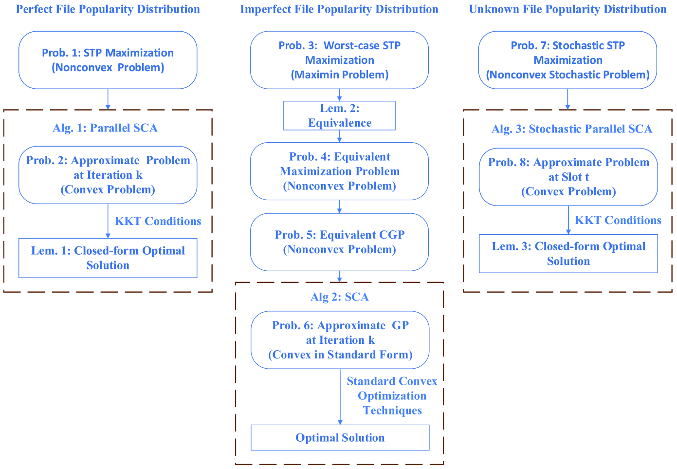
Refer to caption
Figure 2: The optimization problems and corresponding solutions in the cases of perfect, imperfect and unknown file popularity distribution.

In Section III, Section IV and Section V, we shall maximize the STP, the worst-case STP and the stochastic STP in the cases of perfect, imperfect and unknown file popularity distribution, respectively, as shown in Fig 2.111111 Based on the solutions in this paper. we can obtain promising caching designs under multicast at the general usesr density region using the method proposed in our previous work [5, 7].

III Performance Optimization for Perfect File Popularity Distribution

In this section, we consider the case of perfect file popularity distribution. In this case, we would like to maximize the STP, by optimizing the caching probabilities. We formulate the optimal random caching design problem as follows.

Problem 1 (Optimization for Perfect File Popularity Distribution)
q(𝐚)max𝐓superscript𝑞𝐚subscript𝐓\displaystyle q^{*}(\mathbf{a})\triangleq\max_{\mathbf{T}}\quad q(𝐚,𝐓)𝑞𝐚𝐓\displaystyle q\left(\mathbf{a},\mathbf{T}\right)
s.t. (4),(5),italic-(4italic-)italic-(5italic-)\displaystyle\eqref{eqn:T1},\eqref{eqn:T2},

where q(𝐚,𝐓)𝑞𝐚𝐓q\left(\mathbf{a},\mathbf{T}\right) is given by (8).

Problem 1 is equivalent to Problem 0 in [9]. It is non-convex (as the objective function is non-convex in 𝐓𝐓\mathbf{T}), and in [9] a suboptimal solution of it is obtained by solving an approximate convex problem. In the following, we extend the technique in [10] for the case of M=2𝑀2M=2 to the case of M2𝑀2M\geq 2, and develop an efficient parallel iterative algorithm to obtain a stationary point of Problem 1 using parallel SCA. Different from the cyclic computation mechanism in [10], the parallel computation mechanism here can speed up the computation, especially for large M𝑀M. Specifically, this algorithm updates the caching probabilities of the M𝑀M tiers, i.e., 𝐓m(Tm,n)n𝒩subscript𝐓𝑚subscriptsubscript𝑇𝑚𝑛𝑛𝒩\mathbf{T}_{m}\triangleq(T_{m,n})_{n\in\mathcal{N}}, m𝑚m\in\mathcal{M}, at each iteration in a parallel manner, by maximizing M𝑀M approximate functions of q(𝐚,𝐓)𝑞𝐚𝐓q\left(\mathbf{a},\mathbf{T}\right).

For notation convenience, define:

qj(𝐚,𝐓m,𝐓m)n𝒩anTj,nlθl,jTl,n+ηj,subscript𝑞𝑗𝐚subscript𝐓𝑚subscript𝐓𝑚subscript𝑛𝒩subscript𝑎𝑛subscript𝑇𝑗𝑛subscript𝑙subscript𝜃𝑙𝑗subscript𝑇𝑙𝑛subscript𝜂𝑗\displaystyle q_{j}\left(\mathbf{a},\mathbf{T}_{m},\mathbf{T}_{-m}\right)\triangleq\sum_{n\in\mathcal{N}}{\frac{a_{n}T_{j,n}}{\sum_{l\in\mathcal{M}}{\theta_{l,j}T_{l,n}}+\eta_{j}}}, (13)

where 𝐓m(𝐓j)j,jmsubscript𝐓𝑚subscriptsubscript𝐓𝑗formulae-sequence𝑗𝑗𝑚\mathbf{T}_{-m}\triangleq\left(\mathbf{T}_{j}\right)_{j\in\mathcal{M},j\neq m}. Note that q(𝐚,𝐓)𝑞𝐚𝐓q(\mathbf{a},\mathbf{T}) can be rewritten as:

q(𝐚,𝐓m,𝐓m)jqj(𝐚,𝐓m,𝐓m).𝑞𝐚subscript𝐓𝑚subscript𝐓𝑚subscript𝑗subscript𝑞𝑗𝐚subscript𝐓𝑚subscript𝐓𝑚\displaystyle q\left(\mathbf{a},\mathbf{T}_{m},\mathbf{T}_{-m}\right)\triangleq\sum_{j\in\mathcal{M}}q_{j}\left(\mathbf{a},\mathbf{T}_{m},\mathbf{T}_{-m}\right).

Let 𝐓m(k)superscriptsubscript𝐓𝑚𝑘\mathbf{T}_{m}^{(k)} denote the caching probabilities of tier m𝑚m obtained at iteration k𝑘k, and denote 𝐓(k)(𝐓m(k))m𝐌superscript𝐓𝑘subscriptsuperscriptsubscript𝐓𝑚𝑘𝑚𝐌\mathbf{T}^{(k)}\triangleq\big{(}\mathbf{T}_{m}^{(k)}\big{)}_{m\in\mathbf{M}}. At iteration k+1𝑘1k+1, choose:

hm(𝐚,𝐓m,𝐓(k))subscript𝑚𝐚subscript𝐓𝑚superscript𝐓𝑘absent\displaystyle h_{m}\big{(}\mathbf{a},\mathbf{T}_{m},\mathbf{T}^{(k)}\big{)}\triangleq
qm(𝐚,𝐓m,𝐓m(k))+j,jm(qj(𝐚,𝐓m(k),𝐓m(k))n𝒩anθm,jTj,n(k)(Tm,nTm,n(k))(lθl,jTl,n(k)+ηj)2),subscript𝑞𝑚𝐚subscript𝐓𝑚superscriptsubscript𝐓𝑚𝑘subscriptformulae-sequence𝑗𝑗𝑚subscript𝑞𝑗𝐚superscriptsubscript𝐓𝑚𝑘superscriptsubscript𝐓𝑚𝑘subscript𝑛𝒩subscript𝑎𝑛subscript𝜃𝑚𝑗superscriptsubscript𝑇𝑗𝑛𝑘subscript𝑇𝑚𝑛superscriptsubscript𝑇𝑚𝑛𝑘superscriptsubscript𝑙subscript𝜃𝑙𝑗superscriptsubscript𝑇𝑙𝑛𝑘subscript𝜂𝑗2\displaystyle q_{m}\left(\mathbf{a},\mathbf{T}_{m},\mathbf{T}_{-m}^{(k)}\right)+\sum_{j\in\mathcal{M},j\neq m}\left(q_{j}\left(\mathbf{a},\mathbf{T}_{m}^{(k)},\mathbf{T}_{-m}^{(k)}\right)-\sum_{n\in\mathcal{N}}\frac{a_{n}\theta_{m,j}T_{j,n}^{(k)}\left(T_{m,n}-T_{m,n}^{(k)}\right)}{\left({\sum_{l\in\mathcal{M}}{\theta_{l,j}T_{l,n}^{(k)}}+\eta_{j}}\right)^{2}}\right), (14)

as an approximation function of q(𝐚,𝐓)𝑞𝐚𝐓q(\mathbf{a},\mathbf{T}) for updating 𝐓msubscript𝐓𝑚\mathbf{T}_{m}. Note that the strongly concave component function of q(𝐚,𝐓m,𝐓m(k))𝑞𝐚subscript𝐓𝑚superscriptsubscript𝐓𝑚𝑘q\big{(}\mathbf{a},\mathbf{T}_{m},\mathbf{T}_{-m}^{(k)}\big{)}, i.e., qm(𝐚,𝐓m,𝐓m(k))subscript𝑞𝑚𝐚subscript𝐓𝑚superscriptsubscript𝐓𝑚𝑘q_{m}\big{(}\mathbf{a},\mathbf{T}_{m},\mathbf{T}_{-m}^{(k)}\big{)}, is left unchanged, and the other nonconcave (actually convex) component functions, i.e., qj(𝐚,𝐓m,𝐓m(k))subscript𝑞𝑗𝐚subscript𝐓𝑚superscriptsubscript𝐓𝑚𝑘q_{j}\big{(}\mathbf{a},\mathbf{T}_{m},\mathbf{T}_{-m}^{(k)}\big{)}, j𝑗j\in\mathcal{M}, jm𝑗𝑚j\neq m, are linearized at 𝐓m=𝐓m(k)subscript𝐓𝑚superscriptsubscript𝐓𝑚𝑘\mathbf{T}_{m}=\mathbf{T}_{m}^{(k)}. This choice of the approximate function is beneficial from several aspects[10]. Firstly, it can guarantee the convergence of the algorithm to a stationary point of Problem 1, which will be shown in Theorem 1. Secondly, it usually leads to fast convergence of the algorithm by exploiting the partial concavity of the objective function, which will be shown in Fig. 3. Thirdly, it yields a closed-form optimal solution of the optimization problem for each tier at each iteration, which will be shown in Lemma 1, and hence a low-complexity algorithm.

Specifically, at iteration k𝑘k, we first solve the following problem for each tier m𝑚m\in\mathcal{M} separately, in a parallel manner.

Problem 2 (Approximate Convex Problem of Problem 1 for Tier m𝑚m at Iteration k𝑘k)
𝐓¯m(k)argmax𝐓msuperscriptsubscript¯𝐓𝑚𝑘subscriptsubscript𝐓𝑚\displaystyle\overline{\mathbf{T}}_{m}^{(k)}\triangleq\mathop{\arg\max}_{\mathbf{T}_{m}}\ hm(,𝐚,𝐓m,𝐓(k1))\displaystyle h_{m}\big{(},\mathbf{a},\mathbf{T}_{m},\mathbf{T}^{(k-1)}\big{)}
s.t. 0Tm,n1,n𝒩,formulae-sequence0subscript𝑇𝑚𝑛1𝑛𝒩\displaystyle 0\leq T_{m,n}\leq 1,\quad n\in\mathcal{N}, (15)
n𝒩Tm,n=Km.subscript𝑛𝒩subscript𝑇𝑚𝑛subscript𝐾𝑚\displaystyle\sum\limits_{n\in\mathcal{N}}T_{m,n}=K_{m}. (16)

Problem 2 is a convex optimization problem and Slater’s condition is satisfied, implying that strong duality holds. Based on KKT conditions, we can obtain a closed-form optimal solution of Problem 2.

Lemma 1 (Optimal Solution of Problem 2)

For all m𝑚m\in\mathcal{M}, the optimal solution of Problem 2 is given by:

T¯m,n(k)=[1θm,man(l,lmθl,mTl,n(k1)+ηm)νm(k)+j,jmanθm,jTj,n(k1)(lθl,jTl,n(k1)+ηj)2l,lmθl,mTl,n(k1)+ηmθm,m]01,superscriptsubscript¯𝑇𝑚𝑛𝑘subscriptsuperscriptdelimited-[]1subscript𝜃𝑚𝑚subscript𝑎𝑛subscriptformulae-sequence𝑙𝑙𝑚subscript𝜃𝑙𝑚superscriptsubscript𝑇𝑙𝑛𝑘1subscript𝜂𝑚superscriptsubscript𝜈𝑚absent𝑘subscriptformulae-sequence𝑗𝑗𝑚subscript𝑎𝑛subscript𝜃𝑚𝑗superscriptsubscript𝑇𝑗𝑛𝑘1superscriptsubscript𝑙subscript𝜃𝑙𝑗superscriptsubscript𝑇𝑙𝑛𝑘1subscript𝜂𝑗2subscriptformulae-sequence𝑙𝑙𝑚subscript𝜃𝑙𝑚superscriptsubscript𝑇𝑙𝑛𝑘1subscript𝜂𝑚subscript𝜃𝑚𝑚10\displaystyle\overline{T}_{m,n}^{(k)}=\left[\frac{1}{\theta_{m,m}}\sqrt{\frac{a_{n}\left(\sum\limits_{l\in\mathcal{M},l\neq m}\theta_{l,m}T_{l,n}^{(k-1)}+\eta_{m}\right)}{\nu_{m}^{*({k})}+\sum\limits_{j\in\mathcal{M},j\neq m}\frac{a_{n}\theta_{m,j}T_{j,n}^{(k-1)}}{\left({\sum\limits_{l\in\mathcal{M}}{\theta_{l,j}T_{l,n}^{(k-1)}}+\eta_{j}}\right)^{2}}}}-\frac{\sum\limits_{l\in\mathcal{M},l\neq m}\theta_{l,m}T_{l,n}^{(k-1)}+\eta_{m}}{\theta_{m,m}}\right]^{1}_{0}, (17)

where [x]01min{max{x,0},1}subscriptsuperscriptdelimited-[]𝑥10𝑥01[x]^{1}_{0}\triangleq\min\left\{\max\{x,0\},1\right\} and νm(k)superscriptsubscript𝜈𝑚absent𝑘\nu_{m}^{*({k})} is the Lagrange multiplier that satisfies n𝒩T¯m,n(k)=Kmsubscript𝑛𝒩superscriptsubscript¯𝑇𝑚𝑛𝑘subscript𝐾𝑚\sum_{n\in\mathcal{N}}\overline{T}_{m,n}^{(k)}=K_{m}.

Note that νm(k)superscriptsubscript𝜈𝑚absent𝑘\nu_{m}^{*({k})} in Lemma 1 can be efficiently obtained by using bisection search which achieves a desired accuracy ϵitalic-ϵ\epsilon with computational complexity 𝒪(M2Nlog(1/ϵ))𝒪superscript𝑀2𝑁1italic-ϵ\mathcal{O}\left(M^{2}N\log(1/\epsilon)\right). Then, we update the caching probabilities of tier m𝑚m by:

𝐓m(k)=(1γ(k))𝐓m(k1)+γ(k)𝐓¯m(k),superscriptsubscript𝐓𝑚𝑘1superscript𝛾𝑘superscriptsubscript𝐓𝑚𝑘1superscript𝛾𝑘superscriptsubscript¯𝐓𝑚𝑘\displaystyle\mathbf{T}_{m}^{(k)}=(1-\gamma^{(k)})\mathbf{T}_{m}^{(k-1)}+\gamma^{(k)}\overline{\mathbf{T}}_{m}^{(k)}, (18)

where γ(k)superscript𝛾𝑘\gamma^{(k)} is a positive diminishing stepsize satisfying

γ(k)>0,limkγ(k)=0,k=1γ(k)=,k=1(γ(k))2<.formulae-sequencesuperscript𝛾𝑘0formulae-sequencesubscript𝑘superscript𝛾𝑘0formulae-sequencesuperscriptsubscript𝑘1superscript𝛾𝑘superscriptsubscript𝑘1superscriptsuperscript𝛾𝑘2\displaystyle\gamma^{(k)}>0,\quad\lim_{k\to\infty}\gamma^{(k)}=0,\quad\sum_{k=1}^{\infty}\gamma^{(k)}=\infty,\quad\sum_{k=1}^{\infty}\left(\gamma^{(k)}\right)^{2}<\infty. (19)

Finally, the details of the proposed parallel iterative algorithm are summarized in Algorithm 1. Based on [25, Theorem 1], we can show the following result.

Theorem 1 (Convergence of Algorithm 1)

If the stepsize {γ(k)}superscript𝛾𝑘\{\gamma^{(k)}\} satisfies (19), then every limit point of {𝐓(k)}superscript𝐓𝑘\{\mathbf{T}^{(k)}\} generated by Algorithm 1 is a stationary point of Problem 1.

Proof:

Please refer to Appendix A. ∎

Algorithm 1 Obtaining A Stationary Point of Problem 1
1:  initialization: choose any feasible solution 𝐓(0)superscript𝐓0\mathbf{T}^{(0)} of Problem 1 as the initial point, and set k=1𝑘1k=1.
2:  repeat
3:   for all m𝑚m\in\mathcal{M}, compute 𝐓¯m(k)superscriptsubscript¯𝐓𝑚𝑘\overline{\mathbf{T}}_{m}^{(k)} according to (17), and update 𝐓m(k)superscriptsubscript𝐓𝑚𝑘\mathbf{T}_{m}^{(k)} according to (18).
4:   set k=k+1𝑘𝑘1k=k+1.
5:  until some convergence criteria is met.

IV Robust Optimization for Imperfect File Popularity Distribution

In this section, we consider the case of imperfect file popularity distribution. In this case, we would like to maximize the worst-case STP, by optimizing the caching probabilities. We formulate the robust optimal random caching design problem as follows.

Problem 3 (Robust Optimization for Imperfect File Popularity Distribution)
qwtmax𝐓superscriptsubscript𝑞wtsubscript𝐓\displaystyle q_{\text{wt}}^{*}\triangleq\max_{\mathbf{T}}\ min𝐚𝒜q(𝐚,𝐓)=qwt(𝒜,𝐓)subscriptsubscript𝐚𝒜𝑞𝐚𝐓absentsubscript𝑞wt𝒜𝐓\displaystyle\underbrace{\min_{\mathbf{a}\in\mathcal{A}}q(\mathbf{a},\mathbf{T})}_{=q_{\text{wt}}(\mathcal{A},\mathbf{T})}
s.t. (4),(5),italic-(4italic-)italic-(5italic-)\displaystyle\eqref{eqn:T1},\eqref{eqn:T2},

where q(𝐚,𝐓)𝑞𝐚𝐓q(\mathbf{a},\mathbf{T}) is given by (8).

Problem 3 is a challenging maximin problem, which does not lie in the category of convex-concave games that can be easily solved (as q(𝐚,𝐓)𝑞𝐚𝐓q(\mathbf{a},\mathbf{T}) is a nonconcave function of 𝐓𝐓\mathbf{T}). In the following, we solve it in two steps.

Firstly, we transform the maximin problem in Problem 3 to an equivalent maximization problem. As the inner problem min𝐚𝒜q(𝐚,𝐓)subscript𝐚𝒜𝑞𝐚𝐓\min_{\mathbf{a}\in\mathcal{A}}q\left(\mathbf{a},\mathbf{T}\right) is a linear programming (LP) with respect to 𝐚𝐚\mathbf{a} and strong duality holds for LP, the inner problem min𝐚𝒜q(𝐚,𝐓)subscript𝐚𝒜𝑞𝐚𝐓\min_{\mathbf{a}\in\mathcal{A}}q\left(\mathbf{a},\mathbf{T}\right) shares the same optimal value with its dual problem. Thus, we can transform Problem 3 to the following equivalent maximization problem by replacing the inner problem with its dual problem.

Problem 4 (Equivalent Problem of Problem 3)
qwtmax𝐓,𝝀𝟎,𝝁𝟎,νsuperscriptsubscript𝑞wtsubscriptformulae-sequencesucceeds-or-equals𝐓𝝀0succeeds-or-equals𝝁0𝜈\displaystyle q_{\text{wt}}^{\star}\triangleq\max_{\mathbf{T},\boldsymbol{\lambda}\succeq\mathbf{0},\boldsymbol{\mu}\succeq\mathbf{0},{\nu}}\quad n𝒩(λna¯nμna¯n)νsubscript𝑛𝒩subscript𝜆𝑛subscript¯𝑎𝑛subscript𝜇𝑛subscript¯𝑎𝑛𝜈\displaystyle\sum_{n\in\mathcal{N}}{(\lambda_{n}\underline{a}_{n}-\mu_{n}\overline{a}_{n})}-\nu
s.t. (4),(5),italic-(4italic-)italic-(5italic-)\displaystyle\eqref{eqn:T1},\eqref{eqn:T2},
mTm,nlθl,mTl,n+ηm+μnλn+ν=0,n𝒩,formulae-sequencesubscript𝑚subscript𝑇𝑚𝑛subscript𝑙subscript𝜃𝑙𝑚subscript𝑇𝑙𝑛subscript𝜂𝑚subscript𝜇𝑛subscript𝜆𝑛𝜈0𝑛𝒩\displaystyle\sum_{m\in\mathcal{M}}{\frac{T_{m,n}}{\sum_{l\in\mathcal{M}}{\theta_{l,m}T_{l,n}}+\eta_{m}}}+\mu_{n}-\lambda_{n}+\nu=0,\quad n\in\mathcal{N}, (20)

where 𝛌(λn)n𝒩𝛌subscriptsubscript𝜆𝑛𝑛𝒩\boldsymbol{\lambda}\triangleq(\lambda_{n})_{n\in\mathcal{N}} and 𝛍(μn)n𝒩𝛍subscriptsubscript𝜇𝑛𝑛𝒩\boldsymbol{\mu}\triangleq(\mu_{n})_{n\in\mathcal{N}}.

Note that 𝝀𝝀\boldsymbol{\lambda}, 𝝁𝝁\boldsymbol{\mu} and ν𝜈\nu are dual variables for the dual problem of the inner problem, corresponding to ana¯nsubscript𝑎𝑛subscript¯𝑎𝑛a_{n}\geq\underline{a}_{n}, ana¯nsubscript𝑎𝑛subscript¯𝑎𝑛a_{n}\leq\overline{a}_{n}, n𝒩𝑛𝒩n\in\mathcal{N}, and n𝒩an=1subscript𝑛𝒩subscript𝑎𝑛1\sum_{n\in\mathcal{N}}a_{n}=1, respectively.

Lemma 2 (Equivalence between Problem 3 and Problem 4)

Problem 3 and Problem 4 have the same optimal value and optimal caching probabilities.

Proof:

Please refer to Appendix B. ∎

Based on Lemma 2, we can solve Problem 4 instead of Problem 3. Problem 4 is nonconvex, as the constraints in (20) are nonconvex. In what follows, we show how to obtain a stationary point of Problem 4 using SCA. We first rewrite ν𝜈\nu as ν1ν2subscript𝜈1subscript𝜈2\nu_{1}-\nu_{2} with ν1,ν2>0subscript𝜈1subscript𝜈20\nu_{1},\nu_{2}>0, and define new variables 𝐱(xm,n)m,n𝒩𝐱subscriptsubscript𝑥𝑚𝑛formulae-sequence𝑚𝑛𝒩\mathbf{x}\triangleq(x_{m,n})_{m\in\mathcal{M},n\in\mathcal{N}}:121212Note that ηm>0subscript𝜂𝑚0\eta_{m}>0, as B(2α,12α)>0𝐵2𝛼12𝛼0B\left(\frac{2}{\alpha},1-\frac{2}{\alpha}\right)>0, and in most practical cases, θl,m>0subscript𝜃𝑙𝑚0\theta_{l,m}>0 [10]. Thus, in the rest of this paper, we consider the case where xm,n>0subscript𝑥𝑚𝑛0x_{m,n}>0 for all m𝑚m\in\mathcal{M} and n𝒩𝑛𝒩n\in\mathcal{N}.

xm,n=l=1Mθl,mTl,n+ηm,m,n𝒩.formulae-sequencesubscript𝑥𝑚𝑛superscriptsubscript𝑙1𝑀subscript𝜃𝑙𝑚subscript𝑇𝑙𝑛subscript𝜂𝑚formulae-sequence𝑚𝑛𝒩\displaystyle x_{m,n}=\sum_{l=1}^{M}\theta_{l,m}T_{l,n}+\eta_{m},\quad m\in\mathcal{M},n\in\mathcal{N}. (21)

We also introduce a new variable y>0𝑦0y>0 which serves as a lower bound of the objective function of Problem 4:

yn𝒩(λna¯nμna¯n)ν.𝑦subscript𝑛𝒩subscript𝜆𝑛subscript¯𝑎𝑛subscript𝜇𝑛subscript¯𝑎𝑛𝜈\displaystyle y\leq\sum_{n\in\mathcal{N}}{(\lambda_{n}\underline{a}_{n}-\mu_{n}\overline{a}_{n})}-\nu. (22)

Therefore, Problem 4 can be equivalently transformed to the following problem.131313For ease of analysis, in Problem 5, we consider 𝐓0succeeds𝐓0\mathbf{T}\succ 0 instead of 𝐓0succeeds-or-equals𝐓0\mathbf{T}\succeq 0, which does not change the optimal value or affect the numerical solution.

Problem 5 (Equivalent Problem of Problem 4)
max𝐓,𝐱,𝝀,𝝁𝟎ν1,ν2,y>0subscriptsucceeds𝐓𝐱𝝀𝝁0subscript𝜈1subscript𝜈2𝑦0\displaystyle\max_{\begin{subarray}{c}\mathbf{T},\mathbf{x},\boldsymbol{\lambda},\boldsymbol{\mu}\succ\mathbf{0}\\ {\nu_{1}},{\nu_{2}},y>0\end{subarray}}\quad y𝑦\displaystyle y
s.t. y+n𝒩μna¯n+ν1n𝒩λna¯n+ν21,𝑦subscript𝑛𝒩subscript𝜇𝑛subscript¯𝑎𝑛subscript𝜈1subscript𝑛𝒩subscript𝜆𝑛subscript¯𝑎𝑛subscript𝜈21\displaystyle\frac{y+\sum_{n\in\mathcal{N}}{\mu_{n}\overline{a}_{n}}+\nu_{1}}{\sum_{n\in\mathcal{N}}{\lambda_{n}\underline{a}_{n}}+\nu_{2}}\leq 1, (23)
λn+ν2mTm,nxm,n1+μn+ν11,n𝒩,formulae-sequencesubscript𝜆𝑛subscript𝜈2subscript𝑚subscript𝑇𝑚𝑛superscriptsubscript𝑥𝑚𝑛1subscript𝜇𝑛subscript𝜈11𝑛𝒩\displaystyle\frac{\lambda_{n}+\nu_{2}}{\sum_{m\in\mathcal{M}}{T_{m,n}}{x_{m,n}^{-1}}+\mu_{n}+\nu_{1}}\leq 1,\quad n\in\mathcal{N}, (24)
lθl,mTl,n+ηmxm,n1,m,n𝒩,formulae-sequencesubscript𝑙subscript𝜃𝑙𝑚subscript𝑇𝑙𝑛subscript𝜂𝑚subscript𝑥𝑚𝑛1formulae-sequence𝑚𝑛𝒩\displaystyle\frac{\sum_{l\in\mathcal{M}}\theta_{l,m}T_{l,n}+\eta_{m}}{x_{m,n}}\leq 1,\quad m\in\mathcal{M},\ n\in\mathcal{N}, (25)
Tm,n1,m,n𝒩,formulae-sequencesubscript𝑇𝑚𝑛1formulae-sequence𝑚𝑛𝒩\displaystyle T_{m,n}\leq 1,\quad m\in\mathcal{M},\ n\in\mathcal{N}, (26)
n𝒩Tm,nKm,m.formulae-sequencesubscript𝑛𝒩subscript𝑇𝑚𝑛subscript𝐾𝑚𝑚\displaystyle\sum\limits_{n\in\mathcal{N}}T_{m,n}\leq K_{m},\quad m\in\mathcal{M}. (27)

Note that the inequality constraints in (24), (25) and (27) are active at any optimal solution of Problem 5, and hence can replace the equality constraints in (20), (69) and (5), respectively. In Problem 5, a monomial is maximized subject to upper bounds on posynomials (i.e., (25), (26) and (27)) and upper bounds on the ratios of posynomials (i.e., (23) and (24)). Thus, Problem 5 is a CGP, and can be solved by the method proposed in [26], which is based on SCA. The main idea is to solve a sequence of successively refined geometric programmings (GPs), each of which is obtained by approximating the denominators of the ratios of posynomials in (23) and (24) with monomials. Specifically, at iteration k𝑘k, update (𝐓(k),𝐱(k),𝝀(k),𝝁(k),ν1(k),ν2(k),y(k))superscript𝐓𝑘superscript𝐱𝑘superscript𝝀𝑘superscript𝝁𝑘superscriptsubscript𝜈1𝑘superscriptsubscript𝜈2𝑘superscript𝑦𝑘\big{(}\mathbf{T}^{(k)},\mathbf{x}^{(k)},\boldsymbol{\lambda}^{(k)},\boldsymbol{\mu}^{(k)},{\nu_{1}}^{(k)},{\nu_{2}}^{(k)},y^{(k)}\big{)} by solving the following approximate GP of Problem 5, which is parameterized by (𝐓(k1),𝐱(k1),𝝀(k1),𝝁(k1),ν1(k1),ν2(k1))superscript𝐓𝑘1superscript𝐱𝑘1superscript𝝀𝑘1superscript𝝁𝑘1superscriptsubscript𝜈1𝑘1superscriptsubscript𝜈2𝑘1\big{(}\mathbf{T}^{(k-1)},\mathbf{x}^{(k-1)},\boldsymbol{\lambda}^{(k-1)},\boldsymbol{\mu}^{(k-1)},{\nu_{1}}^{(k-1)},{\nu_{2}}^{(k-1)}\big{)} obtained at iteration k1𝑘1k-1.

Problem 6 (Approximate GP at Iteration k𝑘k)
(𝐓(k),𝐱(k),𝝀(k),𝝁(k),ν1(k),ν2(k),y(k))argmax𝐓,𝐱,𝝀,𝝁𝟎ν1,ν2,y>0ysuperscript𝐓𝑘superscript𝐱𝑘superscript𝝀𝑘superscript𝝁𝑘superscriptsubscript𝜈1𝑘superscriptsubscript𝜈2𝑘superscript𝑦𝑘subscriptsucceeds𝐓𝐱𝝀𝝁0subscript𝜈1subscript𝜈2𝑦0𝑦\displaystyle\big{(}\mathbf{T}^{(k)},\mathbf{x}^{(k)},\boldsymbol{\lambda}^{(k)},\boldsymbol{\mu}^{(k)},{\nu_{1}}^{(k)},{\nu_{2}}^{(k)},y^{(k)}\big{)}\triangleq\mathop{\arg\max}_{\begin{subarray}{c}\mathbf{T},\mathbf{x},\boldsymbol{\lambda},\boldsymbol{\mu}\succ\mathbf{0}\\ {\nu_{1}},{\nu_{2}},y>0\end{subarray}}\quad y
s.t. (25),(26),(27),italic-(25italic-)italic-(26italic-)italic-(27italic-)\displaystyle\eqref{eqn:x1},\eqref{eqn:T3},\eqref{eqn:T4},
y+n=1Nμna¯n+ν1n𝒩(λna¯nσn(k))σn(k)(ν2γ1(k))γ1(k)1,𝑦superscriptsubscript𝑛1𝑁subscript𝜇𝑛subscript¯𝑎𝑛subscript𝜈1subscriptproduct𝑛𝒩superscriptsubscript𝜆𝑛subscript¯𝑎𝑛superscriptsubscript𝜎𝑛𝑘superscriptsubscript𝜎𝑛𝑘superscriptsubscript𝜈2superscriptsubscript𝛾1𝑘superscriptsubscript𝛾1𝑘1\displaystyle\frac{y+\sum_{n=1}^{N}{\mu_{n}\overline{a}_{n}}+\nu_{1}}{\prod_{n\in\mathcal{N}}{\left(\frac{\lambda_{n}\underline{a}_{n}}{\sigma_{n}^{(k)}}\right)^{\sigma_{n}^{(k)}}}\left(\frac{\nu_{2}}{\gamma_{1}^{(k)}}\right)^{\gamma_{1}^{(k)}}}\leq 1, (28)
λn+ν2m(Tm,nxm,n1βm,n(k))βm,n(k)(μnγ2,n(k))γ2,n(k)(ν1γ3,n(k))γ3,n(k)1,n𝒩,formulae-sequencesubscript𝜆𝑛subscript𝜈2subscriptproduct𝑚superscriptsubscript𝑇𝑚𝑛superscriptsubscript𝑥𝑚𝑛1superscriptsubscript𝛽𝑚𝑛𝑘superscriptsubscript𝛽𝑚𝑛𝑘superscriptsubscript𝜇𝑛superscriptsubscript𝛾2𝑛𝑘superscriptsubscript𝛾2𝑛𝑘superscriptsubscript𝜈1superscriptsubscript𝛾3𝑛𝑘superscriptsubscript𝛾3𝑛𝑘1𝑛𝒩\displaystyle\frac{\lambda_{n}+\nu_{2}}{\prod_{m\in\mathcal{M}}\left(\frac{T_{m,n}x_{m,n}^{-1}}{\beta_{m,n}^{(k)}}\right)^{\beta_{m,n}^{(k)}}\left(\frac{\mu_{n}}{\gamma_{2,n}^{(k)}}\right)^{\gamma_{2,n}^{(k)}}\left(\frac{\nu_{1}}{\gamma_{3,n}^{(k)}}\right)^{\gamma_{3,n}^{(k)}}}\leq 1,\quad n\in\mathcal{N}, (29)

where

σn(k)superscriptsubscript𝜎𝑛𝑘absent\displaystyle\sigma_{n}^{(k)}\triangleq\ λn(k1)a¯nn𝒩λn(k1)a¯n+ν2(k1),superscriptsubscript𝜆𝑛𝑘1subscript¯𝑎𝑛subscript𝑛𝒩superscriptsubscript𝜆𝑛𝑘1subscript¯𝑎𝑛superscriptsubscript𝜈2𝑘1\displaystyle\frac{\lambda_{n}^{(k-1)}\underline{a}_{n}}{\sum_{n\in\mathcal{N}}{\lambda_{n}^{(k-1)}\underline{a}_{n}}+\nu_{2}^{(k-1)}},
βm,n(k)superscriptsubscript𝛽𝑚𝑛𝑘absent\displaystyle\beta_{m,n}^{(k)}\triangleq\ Tm,n(k1)(xm,n(k1))1mTm,n(k1)(xm,n(k1))1+μn(k1)+ν1(k1),superscriptsubscript𝑇𝑚𝑛𝑘1superscriptsuperscriptsubscript𝑥𝑚𝑛𝑘11subscript𝑚superscriptsubscript𝑇𝑚𝑛𝑘1superscriptsuperscriptsubscript𝑥𝑚𝑛𝑘11superscriptsubscript𝜇𝑛𝑘1superscriptsubscript𝜈1𝑘1\displaystyle\frac{T_{m,n}^{(k-1)}\left(x_{m,n}^{(k-1)}\right)^{-1}}{\sum_{m\in\mathcal{M}}{T_{m,n}^{(k-1)}}{\left(x_{m,n}^{(k-1)}\right)^{-1}}+\mu_{n}^{(k-1)}+\nu_{1}^{(k-1)}},
γ1(k)superscriptsubscript𝛾1𝑘absent\displaystyle\gamma_{1}^{(k)}\triangleq\ ν2(k1)n𝒩λn(k1)a¯n+ν2(k1),superscriptsubscript𝜈2𝑘1subscript𝑛𝒩superscriptsubscript𝜆𝑛𝑘1subscript¯𝑎𝑛superscriptsubscript𝜈2𝑘1\displaystyle\frac{\nu_{2}^{(k-1)}}{\sum_{n\in\mathcal{N}}{\lambda_{n}^{(k-1)}\underline{a}_{n}}+\nu_{2}^{(k-1)}},
γ2,n(k)superscriptsubscript𝛾2𝑛𝑘absent\displaystyle\gamma_{2,n}^{(k)}\triangleq\ μn(k1)mTm,n(k1)(xm,n(k1))1+μn(k1)+ν1(k1),superscriptsubscript𝜇𝑛𝑘1subscript𝑚superscriptsubscript𝑇𝑚𝑛𝑘1superscriptsuperscriptsubscript𝑥𝑚𝑛𝑘11superscriptsubscript𝜇𝑛𝑘1superscriptsubscript𝜈1𝑘1\displaystyle\frac{\mu_{n}^{(k-1)}}{\sum_{m\in\mathcal{M}}{T_{m,n}^{(k-1)}}{\left(x_{m,n}^{(k-1)}\right)^{-1}}+\mu_{n}^{(k-1)}+\nu_{1}^{(k-1)}},
γ3,n(k)superscriptsubscript𝛾3𝑛𝑘absent\displaystyle\gamma_{3,n}^{(k)}\triangleq\ ν1(k1)mTm,n(k1)(xm,n(k1))1+μn(k1)+ν1(k1).superscriptsubscript𝜈1𝑘1subscript𝑚superscriptsubscript𝑇𝑚𝑛𝑘1superscriptsuperscriptsubscript𝑥𝑚𝑛𝑘11superscriptsubscript𝜇𝑛𝑘1superscriptsubscript𝜈1𝑘1\displaystyle\frac{\nu_{1}^{(k-1)}}{\sum_{m\in\mathcal{M}}{T_{m,n}^{(k-1)}}{\left(x_{m,n}^{(k-1)}\right)^{-1}}+\mu_{n}^{(k-1)}+\nu_{1}^{(k-1)}}.

Problem 6 is a standard GP, which can be readily transformed into a convex problem and solved using standard convex optimization techniques, such as the barrier method which achieves a desired accuracy ϵitalic-ϵ\epsilon with computational complexity 𝒪(M3N3log(MN/ϵ))𝒪superscript𝑀3superscript𝑁3𝑀𝑁italic-ϵ\mathcal{O}(M^{3}N^{3}\log(MN/\epsilon)). The details for solving Problem 5 are summarized in Algorithm 2. By the convergence result in [26, Proposition 3], and by comparing the KKT conditions of Problem 4 and Problem 5, we have the following result.

Theorem 2 (Convergence of Algorithm 2)

(𝐓(k)\left(\mathbf{T}^{(k)}\right., 𝐱(k)superscript𝐱𝑘\mathbf{x}^{(k)}, 𝛌(k)superscript𝛌𝑘\boldsymbol{\lambda}^{(k)}, 𝛍(k)superscript𝛍𝑘\boldsymbol{\mu}^{(k)}, ν1(k)superscriptsubscript𝜈1𝑘{\nu_{1}}^{(k)}, ν2(k)superscriptsubscript𝜈2𝑘{\nu_{2}}^{(k)}, y(k))\left.y^{(k)}\right) obtained by Algorithm 2 converges to a stationary point of Problem 5, as k𝑘k\to\infty. Furthermore, the limit point of {(𝐓(k)\left\{\left(\mathbf{T}^{(k)}\right.\right., 𝛌(k)superscript𝛌𝑘\boldsymbol{\lambda}^{(k)}, 𝛍(k)superscript𝛍𝑘\boldsymbol{\mu}^{(k)}, ν1(k)ν2(k))}\left.\left.{\nu_{1}}^{(k)}-{\nu_{2}}^{(k)}\right)\right\} is a stationary point of Problem 4.

Proof:

Please refer to Appendix C. ∎

Algorithm 2 Obtaining A Stationary Point of Problem 5
1:  initialization: choose any feasible solution (𝐓(0)\big{(}\mathbf{T}^{(0)}, 𝐱(0)superscript𝐱0\mathbf{x}^{(0)}, 𝝀(0)superscript𝝀0\boldsymbol{\lambda}^{(0)}, 𝝁(0)superscript𝝁0\boldsymbol{\mu}^{(0)}, ν1(0)superscriptsubscript𝜈10{\nu_{1}}^{(0)}, ν2(0)superscriptsubscript𝜈20{\nu_{2}}^{(0)}, y(0))y^{(0)}\big{)} of Problem 5 as the initial point, and set k=1𝑘1k=1.
2:  repeat
3:   compute (𝐓(k)\big{(}\mathbf{T}^{(k)}, 𝐱(k)superscript𝐱𝑘\mathbf{x}^{(k)}, 𝝀(k)superscript𝝀𝑘\boldsymbol{\lambda}^{(k)}, 𝝁(k)superscript𝝁𝑘\boldsymbol{\mu}^{(k)}, ν1(k)superscriptsubscript𝜈1𝑘{\nu_{1}}^{(k)}, ν2(k)superscriptsubscript𝜈2𝑘{\nu_{2}}^{(k)}, y(k))y^{(k)}\big{)} by transforming Problem 6 into a GP in convex form, and solving it with standard convex optimization techniques.
4:   set k=k+1𝑘𝑘1k=k+1.
5:  until some convergence criteria is met.

V Stochastic Optimization for Unknown File Popularity Distribution

In this section, we consider the case of unknown file popularity distribution. In this case, we would like to maximize the stochastic STP, by optimizing the caching probabilities. We formulate the stochastic optimal random caching design problem as follows.

Problem 7 (Stochastic Optimization for Unknown File Popularity Distribution)
max𝐓subscript𝐓\displaystyle\max_{\mathbf{T}}\quad 𝔼[q(𝝃,𝐓)]=qst(𝐚,𝐓)subscript𝔼delimited-[]𝑞𝝃𝐓absentsubscript𝑞st𝐚𝐓\displaystyle\underbrace{\mathbb{E}\left[q(\boldsymbol{\xi},\mathbf{T})\right]}_{=q_{\text{st}}(\mathbf{a},\mathbf{T})}
s.t. (4),(5),italic-(4italic-)italic-(5italic-)\displaystyle\eqref{eqn:T1},\eqref{eqn:T2},

where q(𝐚,𝐓)𝑞𝐚𝐓q\left(\mathbf{a},\mathbf{T}\right) is given by (8).

Note that although 𝔼[q(𝝃,𝐓)]𝔼delimited-[]𝑞𝝃𝐓\mathbb{E}\left[q(\boldsymbol{\xi},\mathbf{T})\right] cannot be calculated without knowledge of the statistics of 𝝃𝝃\boldsymbol{\xi}, it can be optimized using stochastic optimization.141414The basic idea of stochastic optimization is to optimize a function in the presence of randomness based on the fact that realizations of random parameters can be obtained. Problem 7 is a nonconvex stochastic optimization problem, which is more challenging than a convex one. In the following, we develop an efficient parallel iterative algorithm to obtain a stationary point of Problem 7, using stochastic parallel SCA [27]. Similarly, the parallel computation mechanism here can speed up the computation, especially for large M𝑀M. Specifically, this algorithm updates the caching probabilities of the M𝑀M tiers, i.e., 𝐓m(Tm,n)n𝒩subscript𝐓𝑚subscriptsubscript𝑇𝑚𝑛𝑛𝒩\mathbf{T}_{m}\triangleq(T_{m,n})_{n\in\mathcal{N}}, m𝑚m\in\mathcal{M}, at each slot t𝑡t in a parallel manner, by maximizing M𝑀M approximate functions of qst(𝐚,𝐓)subscript𝑞𝑠𝑡𝐚𝐓q_{st}(\mathbf{a},\mathbf{T}).

Let 𝐓m(t)superscriptsubscript𝐓𝑚𝑡\mathbf{T}_{m}^{(t)} denote the caching probabilities of tier m𝑚m obtained at slot t𝑡t, and denote 𝐓(t)(𝐓m(t))m𝐌superscript𝐓𝑡subscriptsuperscriptsubscript𝐓𝑚𝑡𝑚𝐌\mathbf{T}^{(t)}\triangleq\big{(}\mathbf{T}_{m}^{(t)}\big{)}_{m\in\mathbf{M}}. At slot t𝑡t, choose:

h^m(𝝃(t),𝐓m,𝐓(t1))=ρ(t)(qm(𝝃(t),𝐓m,𝐓m(t1))\displaystyle\widehat{h}_{m}\left(\boldsymbol{\xi}^{(t)},\mathbf{T}_{m},\mathbf{T}^{(t-1)}\right)=\rho^{(t)}\Bigg{(}q_{m}\left(\boldsymbol{\xi}^{(t)},\mathbf{T}_{m},\mathbf{T}_{-m}^{(t-1)}\right)-
j,jmn𝒩ξn(t)θm,j,KjTj,n(t1)(Tm,nTm,n(t1))(lθl,j,KjTl,n(t1)+ηj,Kj)2)+(1ρ(t))n𝒩(Tm,nTm,n(t1))f(t1)m,n\displaystyle\sum_{j\in\mathcal{M},j\neq m}\sum_{n\in\mathcal{N}}\frac{\xi^{(t)}_{n}\theta_{m,j,K_{j}}T_{j,n}^{(t-1)}\left(T_{m,n}-T_{m,n}^{(t-1)}\right)}{\left({\sum_{l\in\mathcal{M}}{\theta_{l,j,K_{j}}T_{l,n}^{(t-1)}}+\eta_{j,K_{j}}}\right)^{2}}\Bigg{)}+(1-\rho^{(t)})\sum_{n\in\mathcal{N}}\left({T}_{m,n}-{T}_{m,n}^{(t-1)}\right){{f}^{(t-1)}_{m,n}} (30)

as an approximation function of qst(𝐚,𝐓)subscript𝑞𝑠𝑡𝐚𝐓q_{st}(\mathbf{a},\mathbf{T}) for updating 𝐓msubscript𝐓𝑚\mathbf{T}_{m}. Here, ξn(t)s𝒰𝐈[πs(t)=n]s𝒰𝐈[πs(t)0]subscriptsuperscript𝜉𝑡𝑛subscript𝑠𝒰𝐈delimited-[]subscriptsuperscript𝜋𝑡𝑠𝑛subscript𝑠𝒰𝐈delimited-[]subscriptsuperscript𝜋𝑡𝑠0\xi^{(t)}_{n}\triangleq\frac{\sum_{s\in\mathcal{U}}\mathbf{I}\left[\pi^{(t)}_{s}=n\right]}{\sum_{s\in\mathcal{U}}\mathbf{I}\left[\pi^{(t)}_{s}\neq 0\right]},151515 We consider a simple way of making use of instantaneous file requests at each slot without assuming any apriori information of the file popularity distribution. Our focus here is to optimize random caching design using stochastic optimization, instead of pure estimation of file popularity. 𝝃(t)(ξn(t))n𝒩superscript𝝃𝑡subscriptsubscriptsuperscript𝜉𝑡𝑛𝑛𝒩\boldsymbol{\xi}^{(t)}\triangleq(\xi^{(t)}_{n})_{n\in\mathcal{N}}, ρ(t)superscript𝜌𝑡\rho^{(t)} is a positive diminishing stepsize satisfying:

ρ(t)>0,limtρ(t)=0,t=1ρ(t)=,t=1(ρ(t))2<,formulae-sequencesuperscript𝜌𝑡0formulae-sequencesubscript𝑡superscript𝜌𝑡0formulae-sequencesuperscriptsubscript𝑡1superscript𝜌𝑡superscriptsubscript𝑡1superscriptsuperscript𝜌𝑡2\displaystyle\rho^{(t)}>0,\quad\lim_{t\to\infty}\rho^{(t)}=0,\quad\sum_{t=1}^{\infty}\rho^{(t)}=\infty,\quad\sum_{t=1}^{\infty}\left(\rho^{(t)}\right)^{2}<\infty, (31)

and fm,n(t)subscriptsuperscript𝑓𝑡𝑚𝑛f^{(t)}_{m,n} is given by:

fm,n(t)=(1ρ(t))fm,n(t1)+ρ(t)(ξnlθl,mTl,n(t)+ηmjξnθm,jTj,n(t)(lθl,jTl,n(t)+ηj)2),subscriptsuperscript𝑓𝑡𝑚𝑛1superscript𝜌𝑡subscriptsuperscript𝑓𝑡1𝑚𝑛superscript𝜌𝑡subscript𝜉𝑛subscript𝑙subscript𝜃𝑙𝑚superscriptsubscript𝑇𝑙𝑛𝑡subscript𝜂𝑚subscript𝑗subscript𝜉𝑛subscript𝜃𝑚𝑗superscriptsubscript𝑇𝑗𝑛𝑡superscriptsubscript𝑙subscript𝜃𝑙𝑗superscriptsubscript𝑇𝑙𝑛𝑡subscript𝜂𝑗2\displaystyle f^{(t)}_{m,n}=(1-\rho^{(t)})f^{(t-1)}_{m,n}+\rho^{(t)}\left(\frac{\xi_{n}}{{\sum_{l\in\mathcal{M}}{\theta_{l,m}T_{l,n}^{(t)}}+\eta_{m}}}-\sum_{j\in\mathcal{M}}\frac{\xi_{n}\theta_{m,j}T_{j,n}^{(t)}}{\left({\sum_{l\in\mathcal{M}}{\theta_{l,j}T_{l,n}^{(t)}}+\eta_{j}}\right)^{2}}\right), (32)

where fm,n(0)=0subscriptsuperscript𝑓0𝑚𝑛0f^{(0)}_{m,n}=0 , m𝑚m\in\mathcal{M}, n𝒩𝑛𝒩n\in\mathcal{N}.

Note that the strongly concave component function of q(𝝃(t),𝐓m,𝐓m(t1))𝑞superscript𝝃𝑡subscript𝐓𝑚superscriptsubscript𝐓𝑚𝑡1q\big{(}\boldsymbol{\xi}^{(t)},\mathbf{T}_{m},\mathbf{T}_{-m}^{(t-1)}\big{)}, i.e., qm(𝝃(t),𝐓m,q_{m}\big{(}\boldsymbol{\xi}^{(t)},\mathbf{T}_{m}, 𝐓m(t1))\mathbf{T}_{-m}^{(t-1)}\big{)}, is left unchanged, and the other nonconcave (actually convex) component functions, i.e., qj(𝝃(t),𝐓m,𝐓m(t1))subscript𝑞𝑗superscript𝝃𝑡subscript𝐓𝑚superscriptsubscript𝐓𝑚𝑡1q_{j}\big{(}\boldsymbol{\xi}^{(t)},\mathbf{T}_{m},\mathbf{T}_{-m}^{(t-1)}\big{)}, j𝑗j\in\mathcal{M}, jm𝑗𝑚j\neq m, are linearized at 𝐓m=𝐓m(t1)subscript𝐓𝑚superscriptsubscript𝐓𝑚𝑡1\mathbf{T}_{m}=\mathbf{T}_{m}^{(t-1)}. In addition, note that the approximation of ansubscript𝑎𝑛a_{n} at each slot t𝑡t, i.e., ξn(t)subscriptsuperscript𝜉𝑡𝑛\xi^{(t)}_{n}, becomes more accurate as s𝒰𝐈[πs(t)0]subscript𝑠𝒰𝐈delimited-[]subscriptsuperscript𝜋𝑡𝑠0{\sum_{s\in\mathcal{U}}\mathbf{I}\left[\pi^{(t)}_{s}\neq 0\right]} increases, and the approximation of Tm,nqst(𝐚,𝐓(t))subscriptsubscript𝑇𝑚𝑛subscript𝑞st𝐚superscript𝐓𝑡\nabla_{{T}_{m,n}}q_{\text{st}}\big{(}\mathbf{a},\mathbf{T}^{(t)}\big{)} based on accumulated instantaneous file requests {πs(t):s𝒰}conditional-setsubscript𝜋𝑠𝑡𝑠𝒰\{\pi_{s}(t):s\in\mathcal{U}\}, t{1,2,,t1}𝑡12𝑡1t\in\{1,2,\dots,t-1\}, i.e., fm,n(t)subscriptsuperscript𝑓𝑡𝑚𝑛{f}^{(t)}_{m,n}, becomes more accurate as t𝑡t increases. This choice of the approximate function, h^m(𝝃(t),𝐓m,𝐓(t1))subscript^𝑚superscript𝝃𝑡subscript𝐓𝑚superscript𝐓𝑡1\widehat{h}_{m}\left(\boldsymbol{\xi}^{(t)},\mathbf{T}_{m},\mathbf{T}^{(t-1)}\right), given in (30), is beneficial for similar reasons as in the case of perfect file popularity distribution.

Specifically, at slot t𝑡t, we first solve the following problem for each tier m𝑚m\in\mathcal{M} separately, in a parallel manner.

Problem 8 (Approximate Convex Problem of Problem 7 for Tier m𝑚m at Slot t𝑡t)
𝐓^m(t)argmax𝐓msuperscriptsubscript^𝐓𝑚𝑡subscriptsubscript𝐓𝑚\displaystyle\widehat{\mathbf{T}}_{m}^{(t)}\triangleq\mathop{\arg\max}_{\mathbf{T}_{m}}\quad h^m(𝝃(t),𝐓m,𝐓(t1))subscript^𝑚superscript𝝃𝑡subscript𝐓𝑚superscript𝐓𝑡1\displaystyle\widehat{h}_{m}\left(\boldsymbol{\xi}^{(t)},\mathbf{T}_{m},\mathbf{T}^{(t-1)}\right)
s.t. (15),(16)italic-(15italic-)italic-(16italic-)\displaystyle\eqref{eqn:Tm1},\eqref{eqn:Tm2}

Problem 8 is a convex optimization problem and Slater’s condition is satisfied, implying that strong duality holds. Based on KKT conditions, we can obtain a closed-form optimal solution of Problem 8.

Lemma 3 (Optimal Solution of Problem 8)

For all m𝑚m\in\mathcal{M}, the optimal solution of Problem 8 is given by:

T^m,n(t)=[1θm,mρ(t)ξn(t)(lm,lθl,mTl,n(t1)+ηm)νm(t)+ρ(t)jmjξn(t)θm,jTj,n(t1)(lθl,jTl,n(t1)+ηj)2(1ρ(t))fm,n(t1)lmlθl,mTl,n(t1)+ηmθm,m]01,superscriptsubscript^𝑇𝑚𝑛𝑡subscriptsuperscriptdelimited-[]1subscript𝜃𝑚𝑚superscript𝜌𝑡subscriptsuperscript𝜉𝑡𝑛subscriptformulae-sequence𝑙𝑚𝑙subscript𝜃𝑙𝑚superscriptsubscript𝑇𝑙𝑛𝑡1subscript𝜂𝑚superscriptsubscript𝜈𝑚absent𝑡superscript𝜌𝑡subscript𝑗𝑚𝑗subscriptsuperscript𝜉𝑡𝑛subscript𝜃𝑚𝑗superscriptsubscript𝑇𝑗𝑛𝑡1superscriptsubscript𝑙subscript𝜃𝑙𝑗superscriptsubscript𝑇𝑙𝑛𝑡1subscript𝜂𝑗21superscript𝜌𝑡subscriptsuperscript𝑓𝑡1𝑚𝑛subscript𝑙𝑚𝑙subscript𝜃𝑙𝑚superscriptsubscript𝑇𝑙𝑛𝑡1subscript𝜂𝑚subscript𝜃𝑚𝑚10\displaystyle\widehat{T}_{m,n}^{(t)}=\left[\frac{1}{\theta_{m,m}}\sqrt{\frac{\rho^{(t)}\xi^{(t)}_{n}\left(\sum\limits_{l\neq m,l\in\mathcal{M}}\theta_{l,m}T_{l,n}^{(t-1)}+\eta_{m}\right)}{\nu_{m}^{*({t})}+\rho^{(t)}\sum\limits_{\begin{subarray}{c}j\neq m\\ j\in\mathcal{M}\end{subarray}}\frac{\xi^{(t)}_{n}\theta_{m,j}T_{j,n}^{(t-1)}}{\left({\sum\limits_{l\in\mathcal{M}}{\theta_{l,j}T_{l,n}^{(t-1)}}+\eta_{j}}\right)^{2}}-(1-\rho^{(t)})f^{(t-1)}_{m,n}}}-\frac{\sum\limits_{\begin{subarray}{c}l\neq m\\ l\in\mathcal{M}\end{subarray}}\theta_{l,m}T_{l,n}^{(t-1)}+\eta_{m}}{\theta_{m,m}}\right]^{1}_{0}, (33)

where [x]01min{max{x,0},1}subscriptsuperscriptdelimited-[]𝑥10𝑥01[x]^{1}_{0}\triangleq\min\left\{\max\{x,0\},1\right\} and νm(t)superscriptsubscript𝜈𝑚absent𝑡\nu_{m}^{*({t})} is the Lagrange multiplier that satisfies n𝒩T^m,n(t)=Kmsubscript𝑛𝒩superscriptsubscript^𝑇𝑚𝑛𝑡subscript𝐾𝑚\sum_{n\in\mathcal{N}}\widehat{T}_{m,n}^{(t)}=K_{m}.

Note that νm(t)superscriptsubscript𝜈𝑚absent𝑡\nu_{m}^{*({t})} in Lemma 3 can be efficiently obtained by using bisection search which achieves a desired accuracy ϵitalic-ϵ\epsilon with computational complexity 𝒪(M2Nlog(1/ϵ))𝒪superscript𝑀2𝑁1italic-ϵ\mathcal{O}\left(M^{2}N\log(1/\epsilon)\right). Then, we update the caching probabilities of tier m𝑚m by:

𝐓m(t)=(1ω(t))𝐓m(t1)+ω(t)𝐓^m(t),superscriptsubscript𝐓𝑚𝑡1superscript𝜔𝑡superscriptsubscript𝐓𝑚𝑡1superscript𝜔𝑡superscriptsubscript^𝐓𝑚𝑡\displaystyle\mathbf{T}_{m}^{(t)}=(1-\omega^{(t)})\mathbf{T}_{m}^{(t-1)}+\omega^{(t)}\widehat{\mathbf{T}}_{m}^{(t)}, (34)

where ω(t)superscript𝜔𝑡\omega^{(t)} is a positive diminishing stepsize satisfying:

ω(t)=0,limtω(t)=0,t=1ω(t)=,t=1(ω(t))2<,limtω(t)ρ(t)=0.formulae-sequencesuperscript𝜔𝑡0formulae-sequencesubscript𝑡superscript𝜔𝑡0formulae-sequencesuperscriptsubscript𝑡1superscript𝜔𝑡formulae-sequencesuperscriptsubscript𝑡1superscriptsuperscript𝜔𝑡2subscript𝑡superscript𝜔𝑡superscript𝜌𝑡0\displaystyle\omega^{(t)}=0,\quad\lim_{t\to\infty}\omega^{(t)}=0,\quad\sum_{t=1}^{\infty}\omega^{(t)}=\infty,\quad\sum_{t=1}^{\infty}\left(\omega^{(t)}\right)^{2}<\infty,\quad\lim_{t\to\infty}\frac{\omega^{(t)}}{\rho^{(t)}}=0. (35)

Finally, the details of the proposed stochastic parallel iterative algorithm are summarized in Algorithm 3.161616Although we assume i.i.d. file request, Algorithm 3 can be applied in the case of time-variant statistics without convergence guarantee. Based on [27, Theorem 1], we can show the following result.

Theorem 3 (Convergence of Algorithm 3)

If the stepsizes {ρ(t)}superscript𝜌𝑡\{\rho^{(t)}\} and {ω(t)}superscript𝜔𝑡\{\omega^{(t)}\} satisfy (31) and (35), respectively, then every limit point of {𝐓(t)}superscript𝐓𝑡\{\mathbf{T}^{(t)}\} generated by Algorithm 3 is almost surely a stationary point of Problem 7.

Proof:

Please refer to Appendix D. ∎

Algorithm 3 Obtaining A Stationary Point of Problem 7
1:  initialization: choose any feasible solution 𝐓(0)superscript𝐓0\mathbf{T}^{(0)} of Problem 7 as the initial point, and set t=1𝑡1t=1.
2:  repeat
3:   observing {πs(t):s𝒰}conditional-setsubscript𝜋𝑠𝑡𝑠𝒰\{\pi_{s}(t):s\in\mathcal{U}\}, and for all m𝑚m\in\mathcal{M}, compute 𝐓^m(t)superscriptsubscript^𝐓𝑚𝑡\widehat{\mathbf{T}}_{m}^{(t)} according to (33), and  update 𝐓m(t)superscriptsubscript𝐓𝑚𝑡\mathbf{T}_{m}^{(t)} according to (34).
4:   set t=t+1𝑡𝑡1t=t+1.
5:  until some convergence criteria is met.

VI Numerical Results

In this section, we show the convergence of the proposed algorithms and compare the proposed algorithms with baseline schemes. We choose M=3𝑀3M=3, N=500𝑁500N=500,171717 Although we choose file number N=500𝑁500N=500 for ease of simulation, numerical results show that the computational time of each proposed algorithm increases approximately linearly with N𝑁N, demonstrating its applicability in practical networks. α=3𝛼3\alpha=3, τ1=1subscript𝜏11\tau_{1}=1, τ2=100.6subscript𝜏2superscript100.6\tau_{2}=10^{-0.6}, τ3=101.4subscript𝜏3superscript101.4\tau_{3}=10^{-1.4}, λ1=3.2×10⁷subscript𝜆13.2superscript107\lambda_{1}=3.2\times 10^{-7}, λ2=8×10⁶subscript𝜆28superscript106\lambda_{2}=8\times 10^{-6}, λ3=8×10⁴subscript𝜆38superscript104\lambda_{3}=8\times 10^{-4}, P1=103P3subscript𝑃1superscript103subscript𝑃3P_{1}=10^{3}P_{3} and P2=101.4P3subscript𝑃2superscript101.4subscript𝑃3P_{2}=10^{1.4}P_{3}. For the case of perfect file popularity distribution, we assume the file popularity follows Zipf distribution, i.e., an=nγn𝒩nγsubscript𝑎𝑛superscript𝑛𝛾subscript𝑛𝒩superscript𝑛𝛾a_{n}=\frac{n^{-\gamma}}{\sum_{n\in\mathcal{N}}n^{-\gamma}}, n𝒩𝑛𝒩n\in\mathcal{N}, where γ𝛾\gamma is the Zipf exponent. For the case of imperfect file popularity distribution, we assume the estimated file popularity is a Zipf distribution, i.e., a^n=nγ^n𝒩nγ^subscript^𝑎𝑛superscript𝑛^𝛾subscript𝑛𝒩superscript𝑛^𝛾\widehat{a}_{n}=\frac{n^{-\widehat{\gamma}}}{\sum_{n\in\mathcal{N}}n^{-\widehat{\gamma}}}, n𝒩𝑛𝒩n\in\mathcal{N}, where γ^^𝛾\widehat{\gamma} is the Zipf exponent, and choose εn=ϵansubscript𝜀𝑛italic-ϵsubscript𝑎𝑛\varepsilon_{n}=\epsilon a_{n}, n𝒩𝑛𝒩n\in\mathcal{N} for some ϵ(0,1)italic-ϵ01\epsilon\in(0,1). For the case of unknown file popularity distribution, we assume that file requests follow the Zipf distribution, i.e., an=nγn𝒩nγsubscript𝑎𝑛superscript𝑛𝛾subscript𝑛𝒩superscript𝑛𝛾a_{n}=\frac{n^{-\gamma}}{\sum_{n\in\mathcal{N}}n^{-\gamma}}, n𝒩𝑛𝒩n\in\mathcal{N}, as in the case of perfect file popularity. In addition, we choose Pr[πs(t)0]=0.9Prdelimited-[]subscript𝜋𝑠𝑡00.9{\rm Pr}[\pi_{s}(t)\neq 0]=0.9. Note that in the simulation, we focus on serving only cached files. When Km/Nsubscript𝐾𝑚𝑁K_{m}/N, m𝑚m\in\mathcal{M} are small, file availability in the M𝑀M-tier network is low, leading to small STPs.

VI-A Convergence

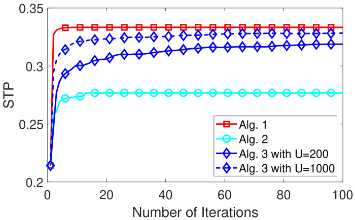
First, we show the convergence of the proposed algorithms. Fig. 3 illustrates the STP, worst-case STP and stochastic STP versus the number of iterations. Although the number of iterations of our proposed algorithms cannot be analytically characterized, from Fig. 3, we can observe that our proposed algorithms terminate in a few iterations. Note that different form Algorithm 1 and Algorithm 2, which are based on the perfect and imperfect popularity distributions at the initial stage, Algorithm 3 can make use of instantaneous file requests observed at each slot and gradually improve the random caching design. In addition, note that Problem 1 and Problem 3 share the same sets of optimal solutions and stationary points, as 𝔼[q(𝝃,𝐓)]=q(𝐚,𝐓)𝔼delimited-[]𝑞𝝃𝐓𝑞𝐚𝐓\mathbb{E}\left[q(\boldsymbol{\xi},\mathbf{T})\right]=q(\mathbf{a},\mathbf{T}). Hence, the converged STPs of Algorithm 1 and Algorithm 3 are similar and are larger than the STP of Algorithm. 2. In addition, Algorithm 3 with a larger U𝑈U converges faster, as at each slot more observations for file requests can be used to approximate the file popularity distribution and the gradient of the stochastic STP.
Refer to caption
Figure 3: STP, Worst-case STP and stochastic STP versus number of iterations in the three cases with K1=80subscript𝐾180K_{1}=80, K2=60subscript𝐾260K_{2}=60, K3=40subscript𝐾340K_{3}=40, γ=γ^=0.55𝛾^𝛾0.55\gamma=\widehat{\gamma}=0.55 and ϵ=0.25italic-ϵ0.25\epsilon=0.25. We choose the same initial point for all the algorithms.

VI-B Performance

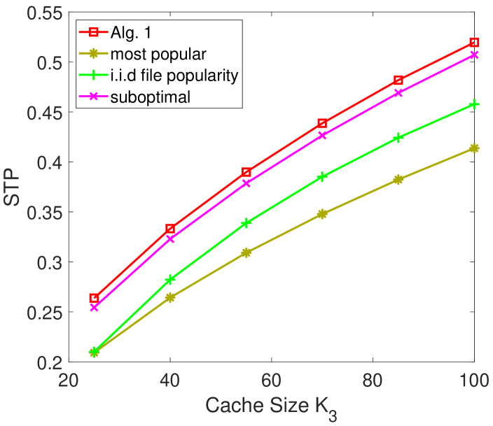
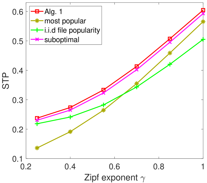
Next, we compare the STP of Algorithm 1 (obtained using 20 iterations), the STP of Algorithm 2 (obtained using 30 iterations) and the STP of Algorithm 3 with U=200𝑈200U=200 (obtained using 200 iterations (slots)) with those of three baseline schemes. Baseline 1 (most popular) refers to the design in which each BS in tier m𝑚m stores the Kmsubscript𝐾𝑚K_{m} most popular files [15] according to 𝐚𝐚{\mathbf{a}} in the case of perfect file popularity distribution, 𝐚^^𝐚\widehat{\mathbf{a}} in the case of imperfect file popularity distribution, and the estimated file popularity 𝐚~(a~n)n𝒩~𝐚subscriptsubscript~𝑎𝑛𝑛𝒩\widetilde{\mathbf{a}}\triangleq(\widetilde{a}_{n})_{n\in\mathcal{N}} in the case of unknown file popularity distribution, where a~nt=1Ls𝒰𝐈[πs(t)=n]t=1Ls𝒰𝐈[πs(t)0]subscript~𝑎𝑛superscriptsubscript𝑡1𝐿subscript𝑠𝒰𝐈delimited-[]subscriptsuperscript𝜋𝑡𝑠𝑛superscriptsubscript𝑡1𝐿subscript𝑠𝒰𝐈delimited-[]subscriptsuperscript𝜋𝑡𝑠0\widetilde{a}_{n}\triangleq\frac{\sum_{t=1}^{L}\sum_{s\in\mathcal{U}}\mathbf{I}\left[\pi^{(t)}_{s}=n\right]}{\sum_{t=1}^{L}\sum_{s\in\mathcal{U}}\mathbf{I}\left[\pi^{(t)}_{s}\neq 0\right]}, n𝒩𝑛𝒩n\in\mathcal{N}, are obtained based on the accumulated file requests within L𝐿L slots. Baseline 2 (i.i.d. file popularity) refers to the design in which each BS in tier m𝑚m randomly stores Kmsubscript𝐾𝑚K_{m} files, in an i.i.d. manner [17] with file n𝑛n being selected with probabilities ansubscript𝑎𝑛{a}_{n} in the case of perfect file popularity distribution, a^nsubscript^𝑎𝑛\widehat{a}_{n} in the case of imperfect file popularity distribution, and a~nsubscript~𝑎𝑛\widetilde{a}_{n} in the case of unknown file popularity distribution. Baseline 3 (suboptimal) refers to the suboptimal caching solution proposed in [9] based on 𝐚nsubscript𝐚𝑛\mathbf{a}_{n} in the case of perfect file popularity distribution, 𝐚^nsubscript^𝐚𝑛\widehat{\mathbf{a}}_{n} in the case of imperfect file popularity distribution, and 𝐚~nsubscript~𝐚𝑛\widetilde{\mathbf{a}}_{n} in the case of unknown file popularity distribution. In addition, we compare with Algorithm 1 based on 𝐚^^𝐚\hat{\mathbf{a}} in the case of imperfect file popularity distribution, referred to as Alg. 1 (imperfect), and with Algorithm 1 based on 𝐚~~𝐚\widetilde{\mathbf{a}} in the case of unknown file popularity, referred to as Alg. 1 (stochastic).181818 Please note that although Baseline 1 (most popular) and Baseline 2 (i.i.d. file popularity) are not optimization-based, they are widely used as baseline schemes in existing works on wireless caching [4, 5, 7, 8, 9, 10]. In addition, note that the proposed solutions in [8] and [10] are for the case of uniform SIR threshold and for a two-tier network, respectively, and hence cannot be applied in our setup.
Refer to caption
(a) cache size K3subscript𝐾3K_{3} at γ=0.55𝛾0.55\gamma=0.55, K1=K3+40subscript𝐾1subscript𝐾340K_{1}=K_{3}+40, K2=K3+20subscript𝐾2subscript𝐾320K_{2}=K_{3}+20.
Refer to caption
(b) Zipf exponent γ𝛾\gamma at K1=80subscript𝐾180K_{1}=80, K2=60subscript𝐾260K_{2}=60, K3=40subscript𝐾340K_{3}=40.
Figure 4: STP versus cache sizes and Zipf exponent γ𝛾\gamma in the case of perfect file popularity distribution.
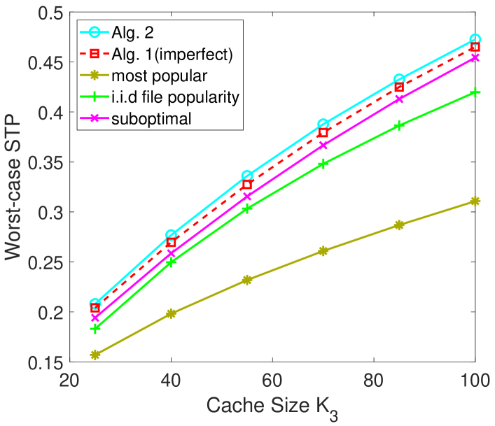
Refer to caption
(a) cache size K3subscript𝐾3K_{3} at γ^=0.55^𝛾0.55\widehat{\gamma}=0.55, ϵ=0.25italic-ϵ0.25\epsilon=0.25, K1=K3+40subscript𝐾1subscript𝐾340K_{1}=K_{3}+40, K2=K3+20subscript𝐾2subscript𝐾320K_{2}=K_{3}+20.
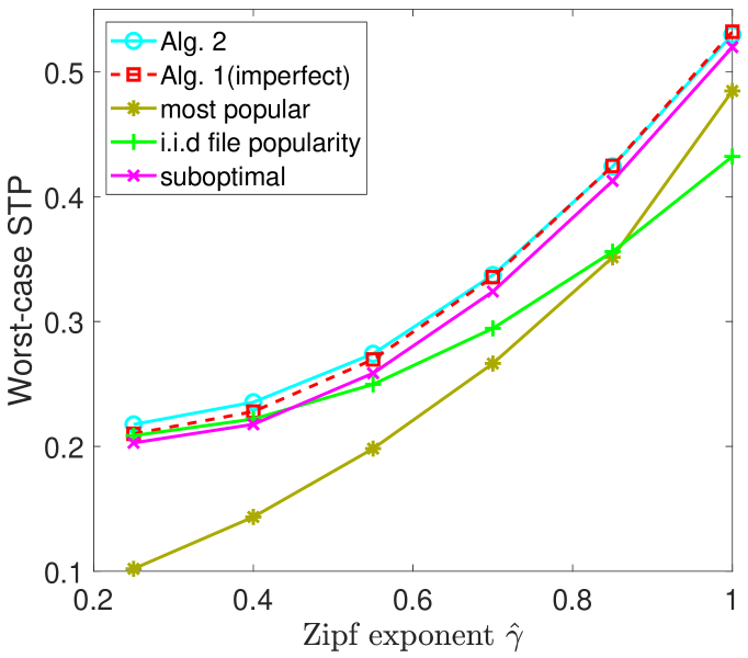
Refer to caption
(b) Zipf exponent γ^^𝛾\widehat{\gamma} at ϵ=0.25italic-ϵ0.25\epsilon=0.25, K1=80subscript𝐾180K_{1}=80, K2=60subscript𝐾260K_{2}=60, K3=40subscript𝐾340K_{3}=40.
Refer to caption
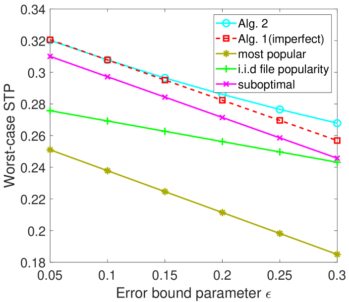
(c) Error bound parameter ϵitalic-ϵ\epsilon at γ^=0.55^𝛾0.55\widehat{\gamma}=0.55, K1=80subscript𝐾180K_{1}=80, K2=60subscript𝐾260K_{2}=60, K3=40subscript𝐾340K_{3}=40.
Figure 5: Worst-case STP versus cache sizes, Zipf exponent γ^^𝛾\widehat{\gamma}, and error bound parameter ϵitalic-ϵ\epsilon in the case of imperfect file popularity distribution.
Refer to caption
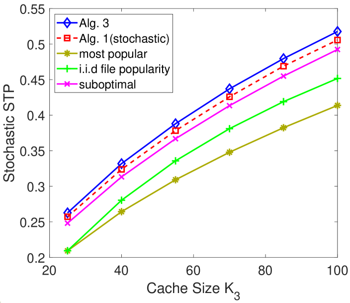
(a) cache size K3subscript𝐾3K_{3} at γ=0.55𝛾0.55\gamma=0.55, L=30𝐿30L=30, K1=K3+40subscript𝐾1subscript𝐾340K_{1}=K_{3}+40, K2=K3+20subscript𝐾2subscript𝐾320K_{2}=K_{3}+20.
Refer to caption
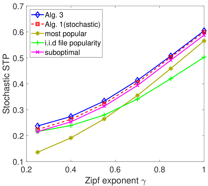
(b) Zipf exponent γ𝛾\gamma at L=30𝐿30L=30, K1=80subscript𝐾180K_{1}=80, K2=60subscript𝐾260K_{2}=60, K3=40subscript𝐾340K_{3}=40.
Refer to caption
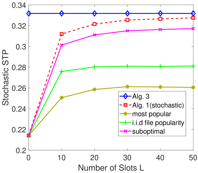
(c) Number of slots L𝐿L at γ=0.55𝛾0.55\gamma=0.55, K1=80subscript𝐾180K_{1}=80, K2=60subscript𝐾260K_{2}=60, K3=40subscript𝐾340K_{3}=40.
Figure 6: Stochastic STP versus cache sizes, Zipf exponent γ𝛾\gamma and number of time slots L𝐿L in the case of unknown file popularity distribution.

Fig. 4(a), Fig. 5(a) and Fig. 6(a) illustrate the STP, the worst-case STP and the stochastic STP versus the cache sizes, respectively. From Fig. 4(a), Fig. 5(a) and Fig. 6(a), we can observe that as the cache sizes Kmsubscript𝐾𝑚K_{m}, m𝑚m\in\mathcal{M} increase, the STP of each scheme increases. This is because as Kmsubscript𝐾𝑚K_{m}, m𝑚m\in\mathcal{M} increase, each BS can cache more files, and the probability that a randomly requested file is cached at a nearby BS increases. In addition, note that for each scheme, its STP in Fig. 4(a) is very close to its stochastic STP in Fig. 6(a), since under the same file popularity distribution, its stochastic STP converges to its STP as the number of iterations goes to infinity.

Fig. 4(b), Fig. 5(b) and Fig. 6(b) illustrate the STP, the worst-case STP and the stochastic STP versus the Zipf exponents, respectively. From Fig. 4(b), Fig. 5(b) and Fig. 6(b), we can observe that as the Zipf exponent γ𝛾\gamma (γ^)^𝛾(\widehat{\gamma}) increases, the STP of each scheme increases. This is because when γ^^𝛾\widehat{\gamma} (γ𝛾\gamma) increases, the tail of the Zipf distribution becomes small, and hence, the probability that a randomly requested file is cached at a nearby BS increases for each scheme. Similarly, note that for each scheme, its STP in Fig. 4(b) is very close to its stochastic STP in Fig. 6(b).

Fig. 5(c) illustrates the worst-case STP versus the error bound parameter ϵitalic-ϵ\epsilon in the case of imperfect file popularity. From Fig. 5(c), we can see that as ϵitalic-ϵ\epsilon increases, the worst-case STP of each scheme decreases. The reason is that as ϵitalic-ϵ\epsilon increases, the possible estimation error increases, and the worst-case STP decreases. In addition, we can observe that the decrease rates of the worst-case STPs of all schemes are different, as the estimation error has different impacts on these schemes. Finally, the STP gaps between Algorithm 2 and the other schemes increase with the error bound parameter, as those schemes do not consider the uncertainty in the file popularity estimation. This reveals the value of robust caching optimization in the case of imperfect file popularity distribution.

Fig. 6(c) illustrates the stochastic STP versus the number of slots L𝐿L which is used for estimating 𝐚~~𝐚\tilde{\mathbf{a}} in the case of unknown file popularity. From Fig. 6(c), we can see that as L𝐿L increases, the stochastic STPs of all schemes except for Algorithm 3 increase. The reason is that as L𝐿L increases, the estimation of the file popularity distribution becomes more accurate. In addition, we can observe that the stochastic STP of Algorithm 3 is not adaptive to L𝐿L, as the proposed solution can be continuously improved by accumulating new file requests. Finally, the STP gaps between Algorithm 3 and the other schemes increase as the number of slots L𝐿L used for estimating 𝐚~~𝐚\tilde{\mathbf{a}} decreases, revealing the value of stochastic caching optimization in the case of unknown file popularity distribution.

Finally, from Fig 4, Fig 5 and Fig 6, we can observe that our proposed solutions outperform the baseline schemes in all three cases. This is because in each case, the properties of the file popularity distribution are appropriately captured when formulating the optimal caching design problem, and a stationary point of the challenging optimization problem is obtained using the proposed algorithm. Note that each point corresponding to the proposed solution in Fig 4, Fig 5 and Fig 6 is obtained with an arbitrary initial point, showing that the performance of a stationary point is promising at least under our setup.

VII Conclusion

In this paper, we considered optimal random caching designs for perfect, imperfect and unknown file popularity distributions in large-scale multi-tier wireless networks. First, in the case of perfect file popularity distribution, we formulate the successful transmission probability (STP) optimization problem, which is nonconvex. We propose an efficient parallel iterative algorithm to obtain a stationary point. Then, in the case of imperfect file popularity distribution, we formulate the worst-case STP maximization problem. This is a challenging robust optimization problem, and we propose an efficient iterative algorithm to obtain a stationary point. Next, in the case of unknown file popularity distribution, we formulate the stochastic STP (i.e., the STP in the stochastic form) maximization problem. This is a challenging nonconvex stochastic optimization problem, and we develop an efficient iterative algorithm to obtain a stationary point. Finally, by numerical results, we show that the proposed solutions achieve notable gains over existing schemes in all three cases.

Appendix A: Proof of Theorem 1

We show that the assumptions in [25, Theorem 1] are satisfied.

  • It is clear that hm(𝐚,𝐓m,𝐓(k))subscript𝑚𝐚subscript𝐓𝑚superscript𝐓𝑘h_{m}\big{(}\mathbf{a},\mathbf{T}_{m},\mathbf{T}^{(k)}\big{)} is continuously differentiable for any given 𝐚𝐚\mathbf{a} and 𝐓(k)superscript𝐓𝑘\mathbf{T}^{(k)}. It remains to show that hm(𝐚,𝐓m,𝐓(k))subscript𝑚𝐚subscript𝐓𝑚superscript𝐓𝑘h_{m}\big{(}\mathbf{a},\mathbf{T}_{m},\mathbf{T}^{(k)}\big{)} is strongly convex in 𝐓msubscript𝐓𝑚\mathbf{T}_{m}. Note that the Hessian of hm(𝐚,𝐓m,𝐓(k))subscript𝑚𝐚subscript𝐓𝑚superscript𝐓𝑘h_{m}\big{(}\mathbf{a},\mathbf{T}_{m},\mathbf{T}^{(k)}\big{)} is 𝐓m2hm(𝐚,𝐓m,𝐓(k))(2hm(𝐚,𝐓m,𝐓(k))Tm,nTm,n)n𝒩,n𝒩subscriptsuperscriptbold-∇2subscript𝐓𝑚subscript𝑚𝐚subscript𝐓𝑚superscript𝐓𝑘subscriptsuperscript2subscript𝑚𝐚subscript𝐓𝑚superscript𝐓𝑘subscript𝑇𝑚𝑛subscript𝑇𝑚superscript𝑛formulae-sequence𝑛𝒩superscript𝑛𝒩\boldsymbol{\nabla}^{2}_{\mathbf{T}_{m}}h_{m}\big{(}\mathbf{a},\mathbf{T}_{m},\mathbf{T}^{(k)}\big{)}\triangleq\Big{(}\frac{\partial^{2}h_{m}\big{(}\mathbf{a},\mathbf{T}_{m},\mathbf{T}^{(k)}\big{)}}{\partial T_{m,n}\partial T_{m,n^{\prime}}}\Big{)}_{n\in\mathcal{N},n^{\prime}\in\mathcal{N}}, where

    2hm(𝐚,𝐓m,𝐓(k))Tm,nTm,n={2anηmθm,m(θm,mTm,n+l,lmθl,mTl,n(k)+ηm)3,n=n,0,nn.superscript2subscript𝑚𝐚subscript𝐓𝑚superscript𝐓𝑘subscript𝑇𝑚𝑛subscript𝑇𝑚superscript𝑛cases2subscript𝑎𝑛subscript𝜂𝑚subscript𝜃𝑚𝑚superscriptsubscript𝜃𝑚𝑚subscript𝑇𝑚𝑛subscriptformulae-sequence𝑙𝑙𝑚subscript𝜃𝑙𝑚subscriptsuperscript𝑇𝑘𝑙𝑛subscript𝜂𝑚3superscript𝑛𝑛0superscript𝑛𝑛\displaystyle\frac{\partial^{2}h_{m}\big{(}\mathbf{a},\mathbf{T}_{m},\mathbf{T}^{(k)}\big{)}}{\partial T_{m,n}\partial T_{m,n^{\prime}}}=\begin{cases}{\frac{-2a_{n}\eta_{m}\theta_{m,m}}{\left({\theta_{m,m}T_{m,n}}+\sum_{l\in\mathcal{M},l\neq m}{\theta_{l,m}T^{(k)}_{l,n}}+\eta_{m}\right)^{3}}},\quad&n^{\prime}=n,\\ 0,\quad&n^{\prime}\neq n.\end{cases} (36)

    Thus, 𝐓m2hm(𝐚,𝐓m,𝐓(k))b𝐄precedes-or-equalssubscriptsuperscriptbold-∇2subscript𝐓𝑚subscript𝑚𝐚subscript𝐓𝑚superscript𝐓𝑘𝑏𝐄\boldsymbol{\nabla}^{2}_{\mathbf{T}_{m}}h_{m}\big{(}\mathbf{a},\mathbf{T}_{m},\mathbf{T}^{(k)}\big{)}\preceq-b\mathbf{E}, where bminn𝒩2anηmθm,m(θm,m+l,lmθl,mTl,n(k)+ηm)3𝑏subscript𝑛𝒩2subscript𝑎𝑛subscript𝜂𝑚subscript𝜃𝑚𝑚superscriptsubscript𝜃𝑚𝑚subscriptformulae-sequence𝑙𝑙𝑚subscript𝜃𝑙𝑚subscriptsuperscript𝑇𝑘𝑙𝑛subscript𝜂𝑚3b\triangleq\min\limits_{n\in\mathcal{N}}{\frac{2a_{n}\eta_{m}\theta_{m,m}}{\left({\theta_{m,m}}+\sum_{l\in\mathcal{M},l\neq m}{\theta_{l,m}T^{(k)}_{l,n}}+\eta_{m}\right)^{3}}}, and 𝐄𝐄\mathbf{E} is the identity matrix. That is, hm(𝐚,𝐓m,𝐓(k))subscript𝑚𝐚subscript𝐓𝑚superscript𝐓𝑘h_{m}\big{(}\mathbf{a},\mathbf{T}_{m},\mathbf{T}^{(k)}\big{)} is uniformly strongly concave with constant b>0𝑏0b>0. Thus, the first assumption of [25, Theorem 1] is satisfied.

  • By (14), we have 𝐓mhm(𝐚,𝐓m,𝐓(k))=𝐓mq(𝐚,𝐓)subscriptsubscript𝐓𝑚subscript𝑚𝐚subscript𝐓𝑚superscript𝐓𝑘subscriptsubscript𝐓𝑚𝑞𝐚𝐓\nabla_{\mathbf{T}_{m}}{h_{m}\big{(}\mathbf{a},\mathbf{T}_{m},\mathbf{T}^{(k)}\big{)}}=\nabla_{\mathbf{T}_{m}}{q\big{(}\mathbf{a},\mathbf{T}\big{)}} for all m𝑚m\in\mathcal{M}. Thus, the second assumption of [25, Theorem 1] is satisfied.

  • It is clear that hm(𝐚,𝐓m,𝐓(k))subscript𝑚𝐚subscript𝐓𝑚superscript𝐓𝑘h_{m}\big{(}\mathbf{a},\mathbf{T}_{m},\mathbf{T}^{(k)}\big{)} is smooth on the constraint set determined by (4) and (5) for any given 𝐚𝐚\mathbf{a} and 𝐓msubscript𝐓𝑚\mathbf{T}_{m}, and hence its derivative is Lipschitz continuous. Thus, the third assumption of [25, Theorem 1] is satisfied.

Therefore, Theorem 3 readily follows from [25, Theorem 1].

Appendix B: Proof of Lemma 2

Firstly, the inner problem of Problem 3, min𝐚𝒜q(𝐚,𝐓)subscript𝐚𝒜subscript𝑞𝐚𝐓\min_{\mathbf{a}\in\mathcal{A}}q_{\infty}\left(\mathbf{a},\mathbf{T}\right), can be rewritten as follows.

Problem 9 (Inner LP of Problem 3)
min𝐚subscript𝐚\displaystyle\min_{\mathbf{a}}\quad q(𝐚,𝐓)𝑞𝐚𝐓\displaystyle q(\mathbf{a},\mathbf{T})
s.t. a¯nan,n𝒩,formulae-sequencesubscript¯𝑎𝑛subscript𝑎𝑛𝑛𝒩\displaystyle\underline{a}_{n}\leq a_{n},\quad n\in\mathcal{N}, (37)
ana¯n,n𝒩,formulae-sequencesubscript𝑎𝑛subscript¯𝑎𝑛𝑛𝒩\displaystyle a_{n}\leq\overline{a}_{n},\quad n\in\mathcal{N}, (38)
n𝒩an=1.subscript𝑛𝒩subscript𝑎𝑛1\displaystyle\sum_{n\in\mathcal{N}}a_{n}=1. (39)

It is clear that Problem 9 is an LP with respect to 𝐚𝐚\mathbf{a} for any given 𝐓𝐓\mathbf{T}, satisfying (4) and (5). From [28, pp.225], we obtain its dual problem as below.

Problem 10 (Dual Problem of Inner LP of Problem 3)
max𝝀,𝝁,νsubscript𝝀𝝁𝜈\displaystyle\max_{\boldsymbol{\lambda},\boldsymbol{\mu},{\nu}}\quad n𝒩(λna¯nμna¯n)νsubscript𝑛𝒩subscript𝜆𝑛subscript¯𝑎𝑛subscript𝜇𝑛subscript¯𝑎𝑛𝜈\displaystyle\sum_{n\in\mathcal{N}}{(\lambda_{n}\underline{a}_{n}-\mu_{n}\overline{a}_{n})}-\nu
s.t. (20),italic-(20italic-)\displaystyle\eqref{eqn:dual1},
λn0,n𝒩,formulae-sequencesubscript𝜆𝑛0𝑛𝒩\displaystyle\lambda_{n}\geq 0,\quad n\in\mathcal{N}, (40)
μn0,n𝒩,formulae-sequencesubscript𝜇𝑛0𝑛𝒩\displaystyle\mu_{n}\geq 0,\quad n\in\mathcal{N}, (41)

where 𝝀𝝀\boldsymbol{\lambda}, 𝝁𝝁\boldsymbol{\mu} and ν𝜈\nu are the Lagrange multipliers corresponding to (37), (38) and (39), respectively.

As strong duality holds for LP, the dual problem in Problem 10 and the primal problem in Problem 9 share the same optimal value, which can be viewed as a function of 𝐓𝐓\mathbf{T}. Thus, the maximin problem in Problem 3 can be equivalently converted to the maximization problem in Problem 4, by replacing the inner LP problem in Problem 9 with its dual problem in Problem 10.

Appendix C: Proof of Theorem 2

By [26, Proposition 3], it can be easily shown that Algorithm 2 converges to a stationary point of Problem 5. Let (𝐓\left(\mathbf{T}^{\star}\right., 𝐱superscript𝐱\mathbf{x}^{\star}, 𝝀superscript𝝀\boldsymbol{\lambda}^{\star}, 𝝁superscript𝝁\boldsymbol{\mu}^{\star}, ν1superscriptsubscript𝜈1{\nu_{1}}^{\star}, ν2,y)\left.{\nu_{2}}^{\star},y^{\star}\right) denote a stationary point of Problem 5, which satisfies the KKT conditions of Problem 5. It remains to show that (𝐓\left(\mathbf{T}^{\star}\right., 𝝀superscript𝝀\boldsymbol{\lambda}^{\star}, 𝝁superscript𝝁\boldsymbol{\mu}^{\star}, ν1ν2)\left.{\nu_{1}}^{\star}-{\nu_{2}}^{\star}\right) is a stationary point of Problem 4, which satisfies the KKT conditions of Problem 4.

First, we derive the KKT conditions of Problem 5 based on its equivalent form given as follows.

Problem 11 (Equivalent Form of Problem 5)
min𝐓,𝐱,𝝀,𝝁,ν1,ν2,ysubscript𝐓𝐱𝝀𝝁subscript𝜈1subscript𝜈2𝑦\displaystyle\min_{{\mathbf{T},\mathbf{x},\boldsymbol{\lambda},\boldsymbol{\mu},{\nu_{1}},{\nu_{2}},y}}\quad y𝑦\displaystyle-y
s.t. (40),(41),italic-(40italic-)italic-(41italic-)\displaystyle\eqref{eqn:dual20},\eqref{eqn:dual30},
yn𝒩(λna¯nμna¯n)+(ν1ν2)0𝑦subscript𝑛𝒩subscript𝜆𝑛subscript¯𝑎𝑛subscript𝜇𝑛subscript¯𝑎𝑛subscript𝜈1subscript𝜈20\displaystyle y-\sum_{n\in\mathcal{N}}{(\lambda_{n}\underline{a}_{n}-\mu_{n}\overline{a}_{n})}+(\nu_{1}-\nu_{2})\leq 0 (42)
λnμn(ν1ν2)mTm,nxm,n10,n𝒩,formulae-sequencesubscript𝜆𝑛subscript𝜇𝑛subscript𝜈1subscript𝜈2subscript𝑚subscript𝑇𝑚𝑛superscriptsubscript𝑥𝑚𝑛10𝑛𝒩\displaystyle\lambda_{n}-\mu_{n}-(\nu_{1}-\nu_{2})-\sum_{m\in\mathcal{M}}{T_{m,n}}{x_{m,n}^{-1}}\leq 0,\quad n\in\mathcal{N}, (43)
(lθl,mTl,n+ηm)xm,n11,m,n𝒩,formulae-sequencesubscript𝑙subscript𝜃𝑙𝑚subscript𝑇𝑙𝑛subscript𝜂𝑚subscriptsuperscript𝑥1𝑚𝑛1formulae-sequence𝑚𝑛𝒩\displaystyle\left({\sum_{l\in\mathcal{M}}\theta_{l,m}T_{l,n}+\eta_{m}}\right){x^{-1}_{m,n}}\leq 1,\quad m\in\mathcal{M},\ n\in\mathcal{N}, (44)
Tm,n0,m,n𝒩,formulae-sequencesubscript𝑇𝑚𝑛0formulae-sequence𝑚𝑛𝒩\displaystyle T_{m,n}\geq 0,\quad m\in\mathcal{M},\ n\in\mathcal{N}, (45)
Tm,n1,m,n𝒩,formulae-sequencesubscript𝑇𝑚𝑛1formulae-sequence𝑚𝑛𝒩\displaystyle T_{m,n}\leq 1,\quad m\in\mathcal{M},\ n\in\mathcal{N}, (46)
n𝒩Tm,nKm,m.formulae-sequencesubscript𝑛𝒩subscript𝑇𝑚𝑛subscript𝐾𝑚𝑚\displaystyle\sum\limits_{n\in\mathcal{N}}T_{m,n}\leq K_{m},\quad m\in\mathcal{M}. (47)

The Lagrangian function of Problem 11 is given by:

(𝐓,𝐱,𝝀,𝝁,ν1,ν2,y,𝝂~1,𝝂~2,λ~0,𝝀~,𝝁~,𝜿~1,𝜿~2,𝜾~)=y+n𝒩ν~1,n(λn)+n𝒩ν~2,n(μn)𝐓𝐱𝝀𝝁subscript𝜈1subscript𝜈2𝑦subscript~𝝂1subscript~𝝂2subscript~𝜆0~𝝀~𝝁subscript~𝜿1subscript~𝜿2~𝜾𝑦subscript𝑛𝒩subscript~𝜈1𝑛subscript𝜆𝑛subscript𝑛𝒩subscript~𝜈2𝑛subscript𝜇𝑛\displaystyle\mathcal{L}\left(\mathbf{T},\mathbf{x},\boldsymbol{\lambda},\boldsymbol{\mu},{\nu_{1}},{\nu_{2}},y,\widetilde{\boldsymbol{\nu}}_{1},\widetilde{\boldsymbol{\nu}}_{2},\widetilde{\lambda}_{0},\widetilde{\boldsymbol{\lambda}},\widetilde{\boldsymbol{\mu}},\widetilde{\boldsymbol{\kappa}}_{1},\widetilde{\boldsymbol{\kappa}}_{2},\widetilde{\boldsymbol{\iota}}\right)=-y+\sum_{n\in\mathcal{N}}\widetilde{\nu}_{1,n}(-\lambda_{n})+\sum_{n\in\mathcal{N}}\widetilde{\nu}_{2,n}(-\mu_{n})
+λ~0(yn𝒩(λna¯nμna¯n)+(ν1ν2))+n𝒩λ~n(λnμn(ν1ν2)mTm,nxm,n1)subscript~𝜆0𝑦subscript𝑛𝒩subscript𝜆𝑛subscript¯𝑎𝑛subscript𝜇𝑛subscript¯𝑎𝑛subscript𝜈1subscript𝜈2subscript𝑛𝒩subscript~𝜆𝑛subscript𝜆𝑛subscript𝜇𝑛subscript𝜈1subscript𝜈2subscript𝑚subscript𝑇𝑚𝑛superscriptsubscript𝑥𝑚𝑛1\displaystyle+\widetilde{\lambda}_{0}\left(y-\sum_{n\in\mathcal{N}}{(\lambda_{n}\underline{a}_{n}-\mu_{n}\overline{a}_{n})}+(\nu_{1}-\nu_{2})\right)+\sum_{n\in\mathcal{N}}\widetilde{\lambda}_{n}\left(\lambda_{n}-\mu_{n}-(\nu_{1}-\nu_{2})-\sum_{m\in\mathcal{M}}{T_{m,n}}{x_{m,n}^{-1}}\right)
+mn𝒩μ~m,n((lθl,mTl,n+ηm)xm,n11)+mι~m(n𝒩Tm,nKm)subscript𝑚subscript𝑛𝒩subscript~𝜇𝑚𝑛subscript𝑙subscript𝜃𝑙𝑚subscript𝑇𝑙𝑛subscript𝜂𝑚subscriptsuperscript𝑥1𝑚𝑛1subscript𝑚subscript~𝜄𝑚subscript𝑛𝒩subscript𝑇𝑚𝑛subscript𝐾𝑚\displaystyle+\sum_{m\in\mathcal{M}}\sum_{n\in\mathcal{N}}\widetilde{\mu}_{m,n}\left(\left({\sum_{l\in\mathcal{M}}\theta_{l,m}T_{l,n}+\eta_{m}}\right){x^{-1}_{m,n}}-1\right)+\sum_{m\in\mathcal{M}}\widetilde{\iota}_{m}\left(\sum\limits_{n\in\mathcal{N}}T_{m,n}-K_{m}\right)
+mn𝒩κ~1,m,n(Tm,n)+mn𝒩κ~2,m,n(Tm,n1),subscript𝑚subscript𝑛𝒩subscript~𝜅1𝑚𝑛subscript𝑇𝑚𝑛subscript𝑚subscript𝑛𝒩subscript~𝜅2𝑚𝑛subscript𝑇𝑚𝑛1\displaystyle+\sum_{m\in\mathcal{M}}\sum_{n\in\mathcal{N}}\widetilde{\kappa}_{1,m,n}(-T_{m,n})+\sum_{m\in\mathcal{M}}\sum_{n\in\mathcal{N}}\widetilde{\kappa}_{2,m,n}(T_{m,n}-1), (48)

where 𝝂~1(ν~1,n)n𝒩subscript~𝝂1subscriptsubscript~𝜈1𝑛𝑛𝒩\widetilde{\boldsymbol{\nu}}_{1}\triangleq(\widetilde{\nu}_{1,n})_{n\in\mathcal{N}}, 𝝂~2(ν~2,n)n𝒩subscript~𝝂2subscriptsubscript~𝜈2𝑛𝑛𝒩\widetilde{\boldsymbol{\nu}}_{2}\triangleq(\widetilde{\nu}_{2,n})_{n\in\mathcal{N}}, λ~0subscript~𝜆0\widetilde{\lambda}_{0}, 𝝀~(λ~n)n𝒩~𝝀subscriptsubscript~𝜆𝑛𝑛𝒩\widetilde{\boldsymbol{\lambda}}\triangleq(\widetilde{\lambda}_{n})_{n\in\mathcal{N}}, 𝝁~(μ~m,n)m,n𝒩~𝝁subscriptsubscript~𝜇𝑚𝑛formulae-sequence𝑚𝑛𝒩\widetilde{\boldsymbol{\mu}}\triangleq(\widetilde{\mu}_{m,n})_{m\in\mathcal{M},n\in\mathcal{N}}, 𝜿~1(κ~1,m,n)m,n𝒩subscript~𝜿1subscriptsubscript~𝜅1𝑚𝑛formulae-sequence𝑚𝑛𝒩\widetilde{\boldsymbol{\kappa}}_{1}\triangleq(\widetilde{\kappa}_{1,m,n})_{m\in\mathcal{M},n\in\mathcal{N}}, 𝜿~2(κ~2,m,n)m,n𝒩subscript~𝜿2subscriptsubscript~𝜅2𝑚𝑛formulae-sequence𝑚𝑛𝒩\widetilde{\boldsymbol{\kappa}}_{2}\triangleq(\widetilde{\kappa}_{2,m,n})_{m\in\mathcal{M},n\in\mathcal{N}} and 𝜾~(ι~m)m~𝜾subscriptsubscript~𝜄𝑚𝑚\widetilde{\boldsymbol{\iota}}\triangleq(\widetilde{\iota}_{m})_{m\in\mathcal{M}} are the Lagrange multipliers corresponding to (40), (41), (42), (43), (44), (45), (46) and (47), respectively.

Next, as (𝐓\left(\mathbf{T}^{\star}\right., 𝐱superscript𝐱\mathbf{x}^{\star}, 𝝀superscript𝝀\boldsymbol{\lambda}^{\star}, 𝝁superscript𝝁\boldsymbol{\mu}^{\star}, ν1superscriptsubscript𝜈1{\nu_{1}}^{\star}, ν2superscriptsubscript𝜈2{\nu_{2}}^{\star}, y)\left.y^{\star}\right) is a stationary point of Problem 5, there exists a dual point (𝝂~1\left(\widetilde{\boldsymbol{\nu}}_{1}^{\star}\right., 𝝂~2superscriptsubscript~𝝂2\widetilde{\boldsymbol{\nu}}_{2}^{\star}, λ~0superscriptsubscript~𝜆0\widetilde{\lambda}_{0}^{\star}, 𝝀~superscript~𝝀\widetilde{\boldsymbol{\lambda}}^{\star}, 𝝁~superscript~𝝁\widetilde{\boldsymbol{\mu}}^{\star}, 𝜿~1superscriptsubscript~𝜿1\widetilde{\boldsymbol{\kappa}}_{1}^{\star}, 𝜿~2superscriptsubscript~𝜿2\widetilde{\boldsymbol{\kappa}}_{2}^{\star}, 𝜾~)\left.\widetilde{\boldsymbol{\iota}}^{\star}\right) together with (𝐓\left(\mathbf{T}^{\star}\right., 𝐱superscript𝐱\mathbf{x}^{\star}, 𝝀superscript𝝀\boldsymbol{\lambda}^{\star}, 𝝁superscript𝝁\boldsymbol{\mu}^{\star}, ν1superscriptsubscript𝜈1{\nu_{1}}^{\star}, ν2superscriptsubscript𝜈2{\nu_{2}}^{\star}, y)\left.y^{\star}\right) satisfies the following KKT conditions:

  • Feasibility: The primal point (𝐓\left(\mathbf{T}^{\star}\right., 𝐱superscript𝐱\mathbf{x}^{\star}, 𝝀superscript𝝀\boldsymbol{\lambda}^{\star}, 𝝁superscript𝝁\boldsymbol{\mu}^{\star}, ν1superscriptsubscript𝜈1{\nu_{1}}^{\star}, ν2,y)\left.{\nu_{2}}^{\star},y^{\star}\right) satisfies the primal constraints in (40), (41), (42), (43), (44), (45), (46) and (47), and the dual point (𝝂~1\left(\widetilde{\boldsymbol{\nu}}_{1}^{\star}\right., 𝝂~2superscriptsubscript~𝝂2\widetilde{\boldsymbol{\nu}}_{2}^{\star}, λ~0superscriptsubscript~𝜆0\widetilde{\lambda}_{0}^{\star}, 𝝀~superscript~𝝀\widetilde{\boldsymbol{\lambda}}^{\star}, 𝝁~superscript~𝝁\widetilde{\boldsymbol{\mu}}^{\star}, 𝜿~1superscriptsubscript~𝜿1\widetilde{\boldsymbol{\kappa}}_{1}^{\star}, 𝜿~2superscriptsubscript~𝜿2\widetilde{\boldsymbol{\kappa}}_{2}^{\star}, 𝜾~)\left.\widetilde{\boldsymbol{\iota}}^{\star}\right) satisfies the dual constraints.

    ν~1,n,ν~2,n,λ~0,λ~n,μ~m,n,κ~1,m,n,κ~2,m,n,ι~m0,m,n𝒩.formulae-sequencesuperscriptsubscript~𝜈1𝑛superscriptsubscript~𝜈2𝑛superscriptsubscript~𝜆0superscriptsubscript~𝜆𝑛superscriptsubscript~𝜇𝑚𝑛superscriptsubscript~𝜅1𝑚𝑛superscriptsubscript~𝜅2𝑚𝑛superscriptsubscript~𝜄𝑚0formulae-sequence𝑚𝑛𝒩\displaystyle\widetilde{\nu}_{1,n}^{\star},\widetilde{\nu}_{2,n}^{\star},\widetilde{\lambda}_{0}^{\star},\widetilde{\lambda}_{n}^{\star},\widetilde{\mu}_{m,n}^{\star},\widetilde{\kappa}_{1,m,n}^{\star},\widetilde{\kappa}_{2,m,n}^{\star},\widetilde{\iota}_{m}^{\star}\geq 0,\quad m\in\mathcal{M},\ n\in\mathcal{N}. (49)
  • Complementary slackness: (𝐓\left(\mathbf{T}^{\star}\right., 𝐱superscript𝐱\mathbf{x}^{\star}, 𝝀superscript𝝀\boldsymbol{\lambda}^{\star}, 𝝁superscript𝝁\boldsymbol{\mu}^{\star}, ν1superscriptsubscript𝜈1{\nu_{1}}^{\star}, ν2,y)\left.{\nu_{2}}^{\star},y^{\star}\right) and (𝝂~1\left(\widetilde{\boldsymbol{\nu}}_{1}^{\star}\right., 𝝂~2superscriptsubscript~𝝂2\widetilde{\boldsymbol{\nu}}_{2}^{\star}, λ~0superscriptsubscript~𝜆0\widetilde{\lambda}_{0}^{\star}, 𝝀~superscript~𝝀\widetilde{\boldsymbol{\lambda}}^{\star}, 𝝁~superscript~𝝁\widetilde{\boldsymbol{\mu}}^{\star}, 𝜿~1superscriptsubscript~𝜿1\widetilde{\boldsymbol{\kappa}}_{1}^{\star}, 𝜿~2superscriptsubscript~𝜿2\widetilde{\boldsymbol{\kappa}}_{2}^{\star}, 𝜾~)\left.\widetilde{\boldsymbol{\iota}}^{\star}\right) satisfy:

    ν~1,nλn=0,n𝒩,formulae-sequencesuperscriptsubscript~𝜈1𝑛superscriptsubscript𝜆𝑛0𝑛𝒩\displaystyle\widetilde{\nu}_{1,n}^{\star}\lambda_{n}^{\star}=0,\quad{n\in\mathcal{N}}, (50)
    ν~2,nμn=0,n𝒩,formulae-sequencesuperscriptsubscript~𝜈2𝑛superscriptsubscript𝜇𝑛0𝑛𝒩\displaystyle\widetilde{\nu}_{2,n}^{\star}\mu_{n}^{\star}=0,\quad{n\in\mathcal{N}}, (51)
    λ~0(yn𝒩(λna¯nμna¯n)+(ν1ν2))=0,superscriptsubscript~𝜆0superscript𝑦subscript𝑛𝒩superscriptsubscript𝜆𝑛subscript¯𝑎𝑛superscriptsubscript𝜇𝑛subscript¯𝑎𝑛superscriptsubscript𝜈1superscriptsubscript𝜈20\displaystyle\widetilde{\lambda}_{0}^{\star}\left(y^{\star}-\sum_{n\in\mathcal{N}}{(\lambda_{n}^{\star}\underline{a}_{n}-\mu_{n}^{\star}\overline{a}_{n})}+(\nu_{1}^{\star}-\nu_{2}^{\star})\right)=0, (52)
    λ~n(λnμn(ν1ν2)mTm,n(xm,n)1)=0,n𝒩,formulae-sequencesuperscriptsubscript~𝜆𝑛superscriptsubscript𝜆𝑛superscriptsubscript𝜇𝑛superscriptsubscript𝜈1superscriptsubscript𝜈2subscript𝑚superscriptsubscript𝑇𝑚𝑛superscriptsuperscriptsubscript𝑥𝑚𝑛10𝑛𝒩\displaystyle\widetilde{\lambda}_{n}^{\star}\left(\lambda_{n}^{\star}-\mu_{n}^{\star}-(\nu_{1}^{\star}-\nu_{2}^{\star})-\sum_{m\in\mathcal{M}}{T_{m,n}^{\star}}({x_{m,n}^{\star}})^{-1}\right)=0,\quad{n\in\mathcal{N}}, (53)
    μ~m,n((lθl,mTl,n+ηm)(xm,n)11)=0,m,n𝒩,formulae-sequencesuperscriptsubscript~𝜇𝑚𝑛subscript𝑙subscript𝜃𝑙𝑚superscriptsubscript𝑇𝑙𝑛subscript𝜂𝑚superscriptsuperscriptsubscript𝑥𝑚𝑛110formulae-sequence𝑚𝑛𝒩\displaystyle\widetilde{\mu}_{m,n}^{\star}\left(\left({\sum_{l\in\mathcal{M}}\theta_{l,m}T_{l,n}^{\star}+\eta_{m}}\right)({x_{m,n}^{\star}})^{-1}-1\right)=0,\quad{m\in\mathcal{M}},\ {n\in\mathcal{N}}, (54)
    κ~1,m,nTm,n=0,m,n𝒩,formulae-sequencesuperscriptsubscript~𝜅1𝑚𝑛superscriptsubscript𝑇𝑚𝑛0formulae-sequence𝑚𝑛𝒩\displaystyle\widetilde{\kappa}_{1,m,n}^{\star}T_{m,n}^{\star}=0,\quad{m\in\mathcal{M}},\ {n\in\mathcal{N}}, (55)
    κ~2,m,n(Tm,n1)=0,m,n𝒩,formulae-sequencesuperscriptsubscript~𝜅2𝑚𝑛superscriptsubscript𝑇𝑚𝑛10formulae-sequence𝑚𝑛𝒩\displaystyle\widetilde{\kappa}_{2,m,n}^{\star}(T_{m,n}^{\star}-1)=0,\quad{m\in\mathcal{M}},\ {n\in\mathcal{N}}, (56)
    ι~m(n𝒩Tm,nKm)=0,m.formulae-sequencesuperscriptsubscript~𝜄𝑚subscript𝑛𝒩superscriptsubscript𝑇𝑚𝑛subscript𝐾𝑚0𝑚\displaystyle\widetilde{\iota}_{m}^{\star}\left(\sum\limits_{n\in\mathcal{N}}T_{m,n}^{\star}-K_{m}\right)=0,\quad{m\in\mathcal{M}}. (57)
  • Zero derivative:

    (𝐓,𝐱,𝝀,𝝁,ν1,ν2,y,𝝂~1,𝝂~2,λ~0,𝝀~,𝝁~,𝜿~1,𝜿~2,𝜾~)y=λ~01=0,superscript𝐓superscript𝐱superscript𝝀superscript𝝁superscriptsubscript𝜈1superscriptsubscript𝜈2superscript𝑦superscriptsubscript~𝝂1superscriptsubscript~𝝂2superscriptsubscript~𝜆0superscript~𝝀superscript~𝝁superscriptsubscript~𝜿1superscriptsubscript~𝜿2superscript~𝜾𝑦superscriptsubscript~𝜆010\displaystyle\frac{\partial\mathcal{L}\left(\mathbf{T}^{\star},\mathbf{x}^{\star},\boldsymbol{\lambda}^{\star},\boldsymbol{\mu}^{\star},{\nu_{1}}^{\star},{\nu_{2}}^{\star},y^{\star},\widetilde{\boldsymbol{\nu}}_{1}^{\star},\widetilde{\boldsymbol{\nu}}_{2}^{\star},\widetilde{\lambda}_{0}^{\star},\widetilde{\boldsymbol{\lambda}}^{\star},\widetilde{\boldsymbol{\mu}}^{\star},\widetilde{\boldsymbol{\kappa}}_{1}^{\star},\widetilde{\boldsymbol{\kappa}}_{2}^{\star},\widetilde{\boldsymbol{\iota}}^{\star}\right)}{\partial y}=\widetilde{\lambda}_{0}^{\star}-1=0, (58)
    (𝐓,𝐱,𝝀,𝝁,ν1,ν2,y,𝝂~1,𝝂~2,λ~0,𝝀~,𝝁~,𝜿~1,𝜿~2,𝜾~)λnsuperscript𝐓superscript𝐱superscript𝝀superscript𝝁superscriptsubscript𝜈1superscriptsubscript𝜈2superscript𝑦superscriptsubscript~𝝂1superscriptsubscript~𝝂2superscriptsubscript~𝜆0superscript~𝝀superscript~𝝁superscriptsubscript~𝜿1superscriptsubscript~𝜿2superscript~𝜾subscript𝜆𝑛\displaystyle\frac{\partial\mathcal{L}\left(\mathbf{T}^{\star},\mathbf{x}^{\star},\boldsymbol{\lambda}^{\star},\boldsymbol{\mu}^{\star},{\nu_{1}}^{\star},{\nu_{2}}^{\star},y^{\star},\widetilde{\boldsymbol{\nu}}_{1}^{\star},\widetilde{\boldsymbol{\nu}}_{2}^{\star},\widetilde{\lambda}_{0}^{\star},\widetilde{\boldsymbol{\lambda}}^{\star},\widetilde{\boldsymbol{\mu}}^{\star},\widetilde{\boldsymbol{\kappa}}_{1}^{\star},\widetilde{\boldsymbol{\kappa}}_{2}^{\star},\widetilde{\boldsymbol{\iota}}^{\star}\right)}{\partial\lambda_{n}}
    =ν~1,nλ~0a¯n+λ~n=0,n𝒩,formulae-sequenceabsentsuperscriptsubscript~𝜈1𝑛superscriptsubscript~𝜆0subscript¯𝑎𝑛superscriptsubscript~𝜆𝑛0𝑛𝒩\displaystyle=-\widetilde{\nu}_{1,n}^{\star}-\widetilde{\lambda}_{0}^{\star}\underline{a}_{n}+\widetilde{\lambda}_{n}^{\star}=0,\quad{n\in\mathcal{N}}, (59)
    (𝐓,𝐱,𝝀,𝝁,ν1,ν2,y,𝝂~1,𝝂~2,λ~0,𝝀~,𝝁~,𝜿~1,𝜿~2,𝜾~)μnsuperscript𝐓superscript𝐱superscript𝝀superscript𝝁superscriptsubscript𝜈1superscriptsubscript𝜈2superscript𝑦superscriptsubscript~𝝂1superscriptsubscript~𝝂2superscriptsubscript~𝜆0superscript~𝝀superscript~𝝁superscriptsubscript~𝜿1superscriptsubscript~𝜿2superscript~𝜾subscript𝜇𝑛\displaystyle\frac{\partial\mathcal{L}\left(\mathbf{T}^{\star},\mathbf{x}^{\star},\boldsymbol{\lambda}^{\star},\boldsymbol{\mu}^{\star},{\nu_{1}}^{\star},{\nu_{2}}^{\star},y^{\star},\widetilde{\boldsymbol{\nu}}_{1}^{\star},\widetilde{\boldsymbol{\nu}}_{2}^{\star},\widetilde{\lambda}_{0}^{\star},\widetilde{\boldsymbol{\lambda}}^{\star},\widetilde{\boldsymbol{\mu}}^{\star},\widetilde{\boldsymbol{\kappa}}_{1}^{\star},\widetilde{\boldsymbol{\kappa}}_{2}^{\star},\widetilde{\boldsymbol{\iota}}^{\star}\right)}{\partial\mu_{n}}
    =ν~2,n+λ~0a¯nλ~n=0,n𝒩,formulae-sequenceabsentsuperscriptsubscript~𝜈2𝑛superscriptsubscript~𝜆0subscript¯𝑎𝑛superscriptsubscript~𝜆𝑛0𝑛𝒩\displaystyle=-\widetilde{\nu}_{2,n}^{\star}+\widetilde{\lambda}_{0}^{\star}\overline{a}_{n}-\widetilde{\lambda}_{n}^{\star}=0,\quad{n\in\mathcal{N}}, (60)
    (𝐓,𝐱,𝝀,𝝁,ν1,ν2,y,𝝂~1,𝝂~2,λ~0,𝝀~,𝝁~,𝜿~1,𝜿~2,𝜾~)ν1=λ~0n𝒩λ~n=0,superscript𝐓superscript𝐱superscript𝝀superscript𝝁superscriptsubscript𝜈1superscriptsubscript𝜈2superscript𝑦superscriptsubscript~𝝂1superscriptsubscript~𝝂2superscriptsubscript~𝜆0superscript~𝝀superscript~𝝁superscriptsubscript~𝜿1superscriptsubscript~𝜿2superscript~𝜾subscript𝜈1superscriptsubscript~𝜆0subscript𝑛𝒩superscriptsubscript~𝜆𝑛0\displaystyle\frac{\partial\mathcal{L}\left(\mathbf{T}^{\star},\mathbf{x}^{\star},\boldsymbol{\lambda}^{\star},\boldsymbol{\mu}^{\star},{\nu_{1}}^{\star},{\nu_{2}}^{\star},y^{\star},\widetilde{\boldsymbol{\nu}}_{1}^{\star},\widetilde{\boldsymbol{\nu}}_{2}^{\star},\widetilde{\lambda}_{0}^{\star},\widetilde{\boldsymbol{\lambda}}^{\star},\widetilde{\boldsymbol{\mu}}^{\star},\widetilde{\boldsymbol{\kappa}}_{1}^{\star},\widetilde{\boldsymbol{\kappa}}_{2}^{\star},\widetilde{\boldsymbol{\iota}}^{\star}\right)}{\partial\nu_{1}}=\widetilde{\lambda}_{0}^{\star}-\sum_{n\in\mathcal{N}}\widetilde{\lambda}_{n}^{\star}=0, (61)
    (𝐓,𝐱,𝝀,𝝁,ν1,ν2,y,𝝂~1,𝝂~2,λ~0,𝝀~,𝝁~,𝜿~1,𝜿~2,𝜾~)xm,nsuperscript𝐓superscript𝐱superscript𝝀superscript𝝁superscriptsubscript𝜈1superscriptsubscript𝜈2superscript𝑦superscriptsubscript~𝝂1superscriptsubscript~𝝂2superscriptsubscript~𝜆0superscript~𝝀superscript~𝝁superscriptsubscript~𝜿1superscriptsubscript~𝜿2superscript~𝜾subscript𝑥𝑚𝑛\displaystyle\frac{\partial\mathcal{L}\left(\mathbf{T}^{\star},\mathbf{x}^{\star},\boldsymbol{\lambda}^{\star},\boldsymbol{\mu}^{\star},{\nu_{1}}^{\star},{\nu_{2}}^{\star},y^{\star},\widetilde{\boldsymbol{\nu}}_{1}^{\star},\widetilde{\boldsymbol{\nu}}_{2}^{\star},\widetilde{\lambda}_{0}^{\star},\widetilde{\boldsymbol{\lambda}}^{\star},\widetilde{\boldsymbol{\mu}}^{\star},\widetilde{\boldsymbol{\kappa}}_{1}^{\star},\widetilde{\boldsymbol{\kappa}}_{2}^{\star},\widetilde{\boldsymbol{\iota}}^{\star}\right)}{\partial x_{m,n}}
    =λ~nTm,nxm,n+μ~m,nxm.n(lθl,mTl,n+ηm)=0,m,n𝒩,formulae-sequenceabsentsuperscriptsubscript~𝜆𝑛superscriptsubscript𝑇𝑚𝑛superscriptsubscript𝑥𝑚𝑛superscriptsubscript~𝜇𝑚𝑛superscriptsubscript𝑥formulae-sequence𝑚𝑛subscript𝑙subscript𝜃𝑙𝑚superscriptsubscript𝑇𝑙𝑛subscript𝜂𝑚0formulae-sequence𝑚𝑛𝒩\displaystyle=-\frac{\widetilde{\lambda}_{n}^{\star}T_{m,n}^{\star}}{x_{m,n}^{\star}}+\frac{\widetilde{\mu}_{m,n}^{\star}}{x_{m.n}^{\star}}{\left({\sum_{l\in\mathcal{M}}\theta_{l,m}T_{l,n}^{\star}+\eta_{m}}\right)}=0,\quad{m\in\mathcal{M}},\ {n\in\mathcal{N}}, (62)
    (𝐓,𝐱,𝝀,𝝁,ν1,ν2,y,𝝂~1,𝝂~2,λ~0,𝝀~,𝝁~,𝜿~1,𝜿~2,𝜾~)Tm,nsuperscript𝐓superscript𝐱superscript𝝀superscript𝝁superscriptsubscript𝜈1superscriptsubscript𝜈2superscript𝑦superscriptsubscript~𝝂1superscriptsubscript~𝝂2superscriptsubscript~𝜆0superscript~𝝀superscript~𝝁superscriptsubscript~𝜿1superscriptsubscript~𝜿2superscript~𝜾subscript𝑇𝑚𝑛\displaystyle\frac{\partial\mathcal{L}\left(\mathbf{T}^{\star},\mathbf{x}^{\star},\boldsymbol{\lambda}^{\star},\boldsymbol{\mu}^{\star},{\nu_{1}}^{\star},{\nu_{2}}^{\star},y^{\star},\widetilde{\boldsymbol{\nu}}_{1}^{\star},\widetilde{\boldsymbol{\nu}}_{2}^{\star},\widetilde{\lambda}_{0}^{\star},\widetilde{\boldsymbol{\lambda}}^{\star},\widetilde{\boldsymbol{\mu}}^{\star},\widetilde{\boldsymbol{\kappa}}_{1}^{\star},\widetilde{\boldsymbol{\kappa}}_{2}^{\star},\widetilde{\boldsymbol{\iota}}^{\star}\right)}{\partial T_{m,n}}
    =λ~n(xm,n)1+lμ~l,nθm,l(xl,n)1κ~1,m,n+κ~2,m,n+ι~m=0,m,n𝒩.formulae-sequenceabsentsuperscriptsubscript~𝜆𝑛superscriptsuperscriptsubscript𝑥𝑚𝑛1subscript𝑙superscriptsubscript~𝜇𝑙𝑛subscript𝜃𝑚𝑙superscriptsuperscriptsubscript𝑥𝑙𝑛1superscriptsubscript~𝜅1𝑚𝑛superscriptsubscript~𝜅2𝑚𝑛superscriptsubscript~𝜄𝑚0formulae-sequence𝑚𝑛𝒩\displaystyle=-\widetilde{\lambda}_{n}^{\star}({x_{m,n}^{\star}})^{-1}+\sum_{l\in\mathcal{M}}\widetilde{\mu}_{l,n}^{\star}\theta_{m,l}({x_{l,n}^{\star}})^{-1}-\widetilde{\kappa}_{1,m,n}^{\star}+\widetilde{\kappa}_{2,m,n}^{\star}+\widetilde{\iota}_{m}^{\star}=0,\quad{m\in\mathcal{M}},\ {n\in\mathcal{N}}. (63)

Then, based on the KKT conditions of Problem 5, we show that the primal point (𝐓\left(\mathbf{T}^{\star}\right., 𝐱superscript𝐱\mathbf{x}^{\star}, 𝝀superscript𝝀\boldsymbol{\lambda}^{\star}, 𝝁superscript𝝁\boldsymbol{\mu}^{\star}, ν1ν2)\left.{\nu_{1}}^{\star}-{\nu_{2}}^{\star}\right) and the dual point (𝝂~1\left(\widetilde{\boldsymbol{\nu}}_{1}^{\star}\right., 𝝂~2superscriptsubscript~𝝂2\widetilde{\boldsymbol{\nu}}_{2}^{\star}, 𝝀~superscript~𝝀\widetilde{\boldsymbol{\lambda}}^{\star}, 𝜿~1superscriptsubscript~𝜿1\widetilde{\boldsymbol{\kappa}}_{1}^{\star}, 𝜿~2superscriptsubscript~𝜿2\widetilde{\boldsymbol{\kappa}}_{2}^{\star}, 𝜾~)\left.\widetilde{\boldsymbol{\iota}}^{\star}\right) satisfy the KKT conditions of Problem 4, implying that (𝐓\left(\mathbf{T}^{\star}\right., 𝝀superscript𝝀\boldsymbol{\lambda}^{\star}, 𝝁superscript𝝁\boldsymbol{\mu}^{\star}, ν1ν2)\left.{\nu_{1}}^{\star}-{\nu_{2}}^{\star}\right) is a stationary point of Problem 4. Note that the Lagrangian function of Problem 4 is given by:

(𝐓,𝝀,𝝁,ν,𝝂~1,𝝂~2,𝝀~,𝜿~1,𝜿~2,𝜾~)=n𝒩(λna¯nμna¯n)+ν𝐓𝝀𝝁𝜈subscript~𝝂1subscript~𝝂2~𝝀subscript~𝜿1subscript~𝜿2~𝜾subscript𝑛𝒩subscript𝜆𝑛subscript¯𝑎𝑛subscript𝜇𝑛subscript¯𝑎𝑛𝜈\displaystyle\mathcal{L}\left(\mathbf{T},\boldsymbol{\lambda},\boldsymbol{\mu},{\nu},\widetilde{\boldsymbol{\nu}}_{1},\widetilde{\boldsymbol{\nu}}_{2},\widetilde{\boldsymbol{\lambda}},\widetilde{\boldsymbol{\kappa}}_{1},\widetilde{\boldsymbol{\kappa}}_{2},\widetilde{\boldsymbol{\iota}}\right)=-\sum_{n\in\mathcal{N}}{(\lambda_{n}\underline{a}_{n}-\mu_{n}\overline{a}_{n})}+\nu
+n𝒩ν~1,n(λn)+n𝒩ν~2,n(μn)+n𝒩λ~n(λnμnνmTm,n(lθl,mTl,n+ηm))subscript𝑛𝒩subscript~𝜈1𝑛subscript𝜆𝑛subscript𝑛𝒩subscript~𝜈2𝑛subscript𝜇𝑛subscript𝑛𝒩subscript~𝜆𝑛subscript𝜆𝑛subscript𝜇𝑛𝜈subscript𝑚subscript𝑇𝑚𝑛subscript𝑙subscript𝜃𝑙𝑚subscript𝑇𝑙𝑛subscript𝜂𝑚\displaystyle+\sum_{n\in\mathcal{N}}\widetilde{\nu}_{1,n}(-\lambda_{n})+\sum_{n\in\mathcal{N}}\widetilde{\nu}_{2,n}(-\mu_{n})+\sum_{n\in\mathcal{N}}\widetilde{\lambda}_{n}\left(\lambda_{n}-\mu_{n}-\nu-\sum_{m\in\mathcal{M}}{\frac{T_{m,n}}{\left({\sum_{l\in\mathcal{M}}\theta_{l,m}T_{l,n}+\eta_{m}}\right)}}\right)
+mn𝒩κ~1,m,n(Tm,n)+mn𝒩κ~2,m,n(Tm,n1)+mι~m(n𝒩Tm,nKm).subscript𝑚subscript𝑛𝒩subscript~𝜅1𝑚𝑛subscript𝑇𝑚𝑛subscript𝑚subscript𝑛𝒩subscript~𝜅2𝑚𝑛subscript𝑇𝑚𝑛1subscript𝑚subscript~𝜄𝑚subscript𝑛𝒩subscript𝑇𝑚𝑛subscript𝐾𝑚\displaystyle+\sum_{m\in\mathcal{M}}\sum_{n\in\mathcal{N}}\widetilde{\kappa}_{1,m,n}(-T_{m,n})+\sum_{m\in\mathcal{M}}\sum_{n\in\mathcal{N}}\widetilde{\kappa}_{2,m,n}(T_{m,n}-1)+\sum_{m\in\mathcal{M}}\widetilde{\iota}_{m}\left(\sum\limits_{n\in\mathcal{N}}T_{m,n}-K_{m}\right). (64)

Now, we prove that the primal point (𝐓\left(\mathbf{T}^{\star}\right., 𝐱superscript𝐱\mathbf{x}^{\star}, 𝝀superscript𝝀\boldsymbol{\lambda}^{\star}, 𝝁superscript𝝁\boldsymbol{\mu}^{\star}, ν1ν2)\left.{\nu_{1}}^{\star}-{\nu_{2}}^{\star}\right) and the dual point (𝝂~1\left(\widetilde{\boldsymbol{\nu}}_{1}^{\star}\right., 𝝂~2superscriptsubscript~𝝂2\widetilde{\boldsymbol{\nu}}_{2}^{\star}, 𝝀~superscript~𝝀\widetilde{\boldsymbol{\lambda}}^{\star}, 𝜿~1superscriptsubscript~𝜿1\widetilde{\boldsymbol{\kappa}}_{1}^{\star}, 𝜿~2superscriptsubscript~𝜿2\widetilde{\boldsymbol{\kappa}}_{2}^{\star}, 𝜾~)\left.\widetilde{\boldsymbol{\iota}}^{\star}\right) satisfy the following KKT conditions.

  • Complementary slackness: It is clear that (𝐓\left(\mathbf{T}^{\star}\right., 𝐱superscript𝐱\mathbf{x}^{\star}, 𝝀superscript𝝀\boldsymbol{\lambda}^{\star}, 𝝁superscript𝝁\boldsymbol{\mu}^{\star}, ν1ν2)\left.{\nu_{1}}^{\star}-{\nu_{2}}^{\star}\right) and (𝝂~1\left(\widetilde{\boldsymbol{\nu}}_{1}^{\star}\right., 𝝂~2superscriptsubscript~𝝂2\widetilde{\boldsymbol{\nu}}_{2}^{\star}, 𝝀~superscript~𝝀\widetilde{\boldsymbol{\lambda}}^{\star}, 𝜿~1superscriptsubscript~𝜿1\widetilde{\boldsymbol{\kappa}}_{1}^{\star}, 𝜿~2superscriptsubscript~𝜿2\widetilde{\boldsymbol{\kappa}}_{2}^{\star}, 𝜾~)\left.\widetilde{\boldsymbol{\iota}}^{\star}\right) satisfy (50), (51), (55) and (56).

  • Zero derivative: Substituting λ~0=1superscriptsubscript~𝜆01\widetilde{\lambda}_{0}^{\star}=1 into (59), (60) and (61), we have:

    (𝐓,𝝀,𝝁,ν,𝝂~1,𝝂~2,𝝀~,𝜿~1,𝜿~2,𝜾~)λn=ν~1,na¯n+λ~n=0,n𝒩,formulae-sequencesuperscript𝐓superscript𝝀superscript𝝁superscript𝜈superscriptsubscript~𝝂1superscriptsubscript~𝝂2superscript~𝝀superscriptsubscript~𝜿1superscriptsubscript~𝜿2superscript~𝜾subscript𝜆𝑛superscriptsubscript~𝜈1𝑛subscript¯𝑎𝑛superscriptsubscript~𝜆𝑛0𝑛𝒩\displaystyle\frac{\partial\mathcal{L}\left(\mathbf{T}^{\star},\boldsymbol{\lambda}^{\star},\boldsymbol{\mu}^{\star},{\nu}^{\star},\widetilde{\boldsymbol{\nu}}_{1}^{\star},\widetilde{\boldsymbol{\nu}}_{2}^{\star},\widetilde{\boldsymbol{\lambda}}^{\star},\widetilde{\boldsymbol{\kappa}}_{1}^{\star},\widetilde{\boldsymbol{\kappa}}_{2}^{\star},\widetilde{\boldsymbol{\iota}}^{\star}\right)}{\partial\lambda_{n}}=-\widetilde{\nu}_{1,n}^{\star}-\underline{a}_{n}+\widetilde{\lambda}_{n}^{\star}=0,\quad{n\in\mathcal{N}}, (65)
    (𝐓,𝝀,𝝁,ν,𝝂~1,𝝂~2,𝝀~,𝜿~1,𝜿~2,𝜾~)μn=ν~2,n+a¯nλ~n=0,n𝒩.formulae-sequencesuperscript𝐓superscript𝝀superscript𝝁superscript𝜈superscriptsubscript~𝝂1superscriptsubscript~𝝂2superscript~𝝀superscriptsubscript~𝜿1superscriptsubscript~𝜿2superscript~𝜾subscript𝜇𝑛superscriptsubscript~𝜈2𝑛subscript¯𝑎𝑛superscriptsubscript~𝜆𝑛0𝑛𝒩\displaystyle\frac{\partial\mathcal{L}\left(\mathbf{T}^{\star},\boldsymbol{\lambda}^{\star},\boldsymbol{\mu}^{\star},{\nu}^{\star},\widetilde{\boldsymbol{\nu}}_{1}^{\star},\widetilde{\boldsymbol{\nu}}_{2}^{\star},\widetilde{\boldsymbol{\lambda}}^{\star},\widetilde{\boldsymbol{\kappa}}_{1}^{\star},\widetilde{\boldsymbol{\kappa}}_{2}^{\star},\widetilde{\boldsymbol{\iota}}^{\star}\right)}{\partial\mu_{n}}=-\widetilde{\nu}_{2,n}^{\star}+\overline{a}_{n}-\widetilde{\lambda}_{n}^{\star}=0,\quad{n\in\mathcal{N}}. (66)
    (𝐓,𝝀,𝝁,ν,𝝂~1,𝝂~2,𝝀~,𝜿~1,𝜿~2,𝜾~)ν=1n𝒩λ~n=0.superscript𝐓superscript𝝀superscript𝝁superscript𝜈superscriptsubscript~𝝂1superscriptsubscript~𝝂2superscript~𝝀superscriptsubscript~𝜿1superscriptsubscript~𝜿2superscript~𝜾𝜈1subscript𝑛𝒩superscriptsubscript~𝜆𝑛0\displaystyle\frac{\partial\mathcal{L}\left(\mathbf{T}^{\star},\boldsymbol{\lambda}^{\star},\boldsymbol{\mu}^{\star},{\nu}^{\star},\widetilde{\boldsymbol{\nu}}_{1}^{\star},\widetilde{\boldsymbol{\nu}}_{2}^{\star},\widetilde{\boldsymbol{\lambda}}^{\star},\widetilde{\boldsymbol{\kappa}}_{1}^{\star},\widetilde{\boldsymbol{\kappa}}_{2}^{\star},\widetilde{\boldsymbol{\iota}}^{\star}\right)}{\partial\nu}=1-\sum_{n\in\mathcal{N}}\widetilde{\lambda}_{n}^{\star}=0. (67)

    Substitute λ~0=1superscriptsubscript~𝜆01\widetilde{\lambda}_{0}^{\star}=1 into (59), we have λ~n=a¯n+ν~1,n>0superscriptsubscript~𝜆𝑛subscript¯𝑎𝑛superscriptsubscript~𝜈1𝑛0\widetilde{\lambda}_{n}^{\star}=\underline{a}_{n}+\widetilde{\nu}_{1,n}^{\star}>0. By λ~n>0superscriptsubscript~𝜆𝑛0\widetilde{\lambda}_{n}^{\star}>0 and (62), we have

    μ~m,n=λ~nTm,n(lθl,mTl,n+ηm)>0.superscriptsubscript~𝜇𝑚𝑛subscript~𝜆𝑛superscriptsubscript𝑇𝑚𝑛subscript𝑙subscript𝜃𝑙𝑚superscriptsubscript𝑇𝑙𝑛subscript𝜂𝑚0\displaystyle\widetilde{\mu}_{m,n}^{\star}=\frac{\widetilde{\lambda}_{n}T_{m,n}^{\star}}{\left({\sum_{l\in\mathcal{M}}\theta_{l,m}T_{l,n}^{\star}+\eta_{m}}\right)}>0. (68)

    In addtion, by μ~m,n>0superscriptsubscript~𝜇𝑚𝑛0\widetilde{\mu}_{m,n}^{\star}>0 and (54), we have

    xm,n=(lθl,mTl,n+ηm).subscriptsuperscript𝑥𝑚𝑛subscript𝑙subscript𝜃𝑙𝑚superscriptsubscript𝑇𝑙𝑛subscript𝜂𝑚\displaystyle{x^{\star}_{m,n}}=\left({\sum_{l\in\mathcal{M}}\theta_{l,m}T_{l,n}^{\star}+\eta_{m}}\right). (69)

    Substituting (68) and (69) into (63), we have:

    (𝐓,𝝀,𝝁,ν,𝝂~1,𝝂~2,𝝀~,𝜿~1,𝜿~2,𝜾~)Tm,nsuperscript𝐓superscript𝝀superscript𝝁superscript𝜈superscriptsubscript~𝝂1superscriptsubscript~𝝂2superscript~𝝀superscriptsubscript~𝜿1superscriptsubscript~𝜿2superscript~𝜾subscript𝑇𝑚𝑛\displaystyle\frac{\partial\mathcal{L}\left(\mathbf{T}^{\star},\boldsymbol{\lambda}^{\star},\boldsymbol{\mu}^{\star},{\nu}^{\star},\widetilde{\boldsymbol{\nu}}_{1}^{\star},\widetilde{\boldsymbol{\nu}}_{2}^{\star},\widetilde{\boldsymbol{\lambda}}^{\star},\widetilde{\boldsymbol{\kappa}}_{1}^{\star},\widetilde{\boldsymbol{\kappa}}_{2}^{\star},\widetilde{\boldsymbol{\iota}}^{\star}\right)}{\partial T_{m,n}}
    =λ~nTm,nTm,n(lθl,mTl,n+ηm)κ~1,m,n+κ~2,m,n+ι~m=0,m,n𝒩.formulae-sequenceabsentsuperscriptsubscript~𝜆𝑛subscriptsubscript𝑇𝑚𝑛superscriptsubscript𝑇𝑚𝑛subscript𝑙subscript𝜃𝑙𝑚superscriptsubscript𝑇𝑙𝑛subscript𝜂𝑚superscriptsubscript~𝜅1𝑚𝑛superscriptsubscript~𝜅2𝑚𝑛superscriptsubscript~𝜄𝑚0formulae-sequence𝑚𝑛𝒩\displaystyle=-\widetilde{\lambda}_{n}^{\star}\nabla_{T_{m,n}}\frac{T_{m,n}^{\star}}{\left({\sum_{l\in\mathcal{M}}\theta_{l,m}T_{l,n}^{\star}+\eta_{m}}\right)}-\widetilde{\kappa}_{1,m,n}^{\star}+\widetilde{\kappa}_{2,m,n}^{\star}+\widetilde{\iota}_{m}^{\star}=0,\ {m\in\mathcal{M}},\ {n\in\mathcal{N}}. (70)

    Note that (65), (66), (67) and (70) are the zero derivative conditions of Problem 4.

  • Feasibility: Given (40), (41), (45), (46) and (49), to show that (𝐓\left(\mathbf{T}^{\star}\right., 𝐱superscript𝐱\mathbf{x}^{\star}, 𝝀superscript𝝀\boldsymbol{\lambda}^{\star}, 𝝁superscript𝝁\boldsymbol{\mu}^{\star}, ν1ν2)\left.{\nu_{1}}^{\star}-{\nu_{2}}^{\star}\right) and (𝝂~1\left(\widetilde{\boldsymbol{\nu}}_{1}^{\star}\right., 𝝂~2superscriptsubscript~𝝂2\widetilde{\boldsymbol{\nu}}_{2}^{\star}, 𝝀~superscript~𝝀\widetilde{\boldsymbol{\lambda}}^{\star}, 𝜿~1superscriptsubscript~𝜿1\widetilde{\boldsymbol{\kappa}}_{1}^{\star}, 𝜿~2superscriptsubscript~𝜿2\widetilde{\boldsymbol{\kappa}}_{2}^{\star}, 𝜾~)\left.\widetilde{\boldsymbol{\iota}}^{\star}\right) satisfy the feasibility conditions of Problem 4, it remains to show:

    mTm,nlθl,mTl,n+ηm+μnλn+ν1ν2=0,n𝒩,formulae-sequencesubscript𝑚superscriptsubscript𝑇𝑚𝑛subscript𝑙subscript𝜃𝑙𝑚superscriptsubscript𝑇𝑙𝑛subscript𝜂𝑚superscriptsubscript𝜇𝑛superscriptsubscript𝜆𝑛subscriptsuperscript𝜈1subscriptsuperscript𝜈20𝑛𝒩\displaystyle\sum_{m\in\mathcal{M}}{\frac{T_{m,n}^{\star}}{\sum_{l\in\mathcal{M}}{\theta_{l,m}T_{l,n}^{\star}}+\eta_{m}}}+\mu_{n}^{\star}-\lambda_{n}^{\star}+\nu^{\star}_{1}-\nu^{\star}_{2}=0,\quad n\in\mathcal{N}, (71)
    n𝒩Tm,n=Km,m.formulae-sequencesubscript𝑛𝒩superscriptsubscript𝑇𝑚𝑛subscript𝐾𝑚𝑚\displaystyle\sum\limits_{n\in\mathcal{N}}T_{m,n}^{\star}=K_{m},\quad m\in\mathcal{M}. (72)

    Note that (71) can be easily shown by λ~n>0superscriptsubscript~𝜆𝑛0\widetilde{\lambda}_{n}^{\star}>0, (53) and (69). Now, we show (72) as below. If κ~2,m,n0superscriptsubscript~𝜅2𝑚𝑛0\widetilde{\kappa}_{2,m,n}^{\star}\neq 0 for all n𝒩𝑛𝒩n\in\mathcal{N}, by (56), we have Tm,n=1subscriptsuperscript𝑇𝑚𝑛1T^{\star}_{m,n}=1 for all n𝒩𝑛𝒩n\in\mathcal{N}, implying n𝒩Tm,n=Nsubscript𝑛𝒩subscriptsuperscript𝑇𝑚𝑛𝑁\sum_{n\in\mathcal{N}}T^{\star}_{m,n}=N, which is contradictory with n𝒩Tm,nKmsubscript𝑛𝒩subscriptsuperscript𝑇𝑚𝑛subscript𝐾𝑚\sum_{n\in\mathcal{N}}T^{\star}_{m,n}\leq K_{m}. Thus, there exists n𝒩𝑛𝒩n\in\mathcal{N}, such that κ~2,m,n=0superscriptsubscript~𝜅2𝑚𝑛0\widetilde{\kappa}_{2,m,n}^{\star}=0. Substituting κ~2,m,n=0superscriptsubscript~𝜅2𝑚𝑛0\widetilde{\kappa}_{2,m,n}^{\star}=0 into (70)italic-(70italic-)\eqref{eqn:deri-40}, we have:

    ι~m=λ~nTm,nTm,n(lθl,mTl,n+ηm)+κ~1,m,n>0.superscriptsubscript~𝜄𝑚superscriptsubscript~𝜆𝑛subscriptsubscript𝑇𝑚𝑛superscriptsubscript𝑇𝑚𝑛subscript𝑙subscript𝜃𝑙𝑚superscriptsubscript𝑇𝑙𝑛subscript𝜂𝑚superscriptsubscript~𝜅1𝑚𝑛0\displaystyle\widetilde{\iota}_{m}^{\star}=\widetilde{\lambda}_{n}^{\star}\nabla_{T_{m,n}}\frac{T_{m,n}^{\star}}{\left({\sum_{l\in\mathcal{M}}\theta_{l,m}T_{l,n}^{\star}+\eta_{m}}\right)}+\widetilde{\kappa}_{1,m,n}^{\star}>0.

    By ι~m>0superscriptsubscript~𝜄𝑚0\widetilde{\iota}_{m}^{\star}>0 and (57), we have (72).

Therefore, (𝐓\left(\mathbf{T}^{\star}\right., 𝐱superscript𝐱\mathbf{x}^{\star}, 𝝀superscript𝝀\boldsymbol{\lambda}^{\star}, 𝝁superscript𝝁\boldsymbol{\mu}^{\star}, ν1ν2)\left.{\nu_{1}}^{\star}-{\nu_{2}}^{\star}\right) and (𝝂~1\left(\widetilde{\boldsymbol{\nu}}_{1}^{\star}\right., 𝝂~2superscriptsubscript~𝝂2\widetilde{\boldsymbol{\nu}}_{2}^{\star}, 𝝀~superscript~𝝀\widetilde{\boldsymbol{\lambda}}^{\star}, 𝜿~1superscriptsubscript~𝜿1\widetilde{\boldsymbol{\kappa}}_{1}^{\star}, 𝜿~2superscriptsubscript~𝜿2\widetilde{\boldsymbol{\kappa}}_{2}^{\star}, 𝜾~)\left.\widetilde{\boldsymbol{\iota}}^{\star}\right) satisfy the KKT conditions of Problem 4.

Appendix D: Proof of Theorem 3

We show that the assumptions in [27, Theorem 1] are satisfied.

  • The constraint set of Problem 7 determined by (4) and (5) is compact and convex. Thus, Assumption a) in [27, Theorem 1] is satisfied.

  • It is clear that qm(𝝃,𝐓)subscript𝑞𝑚𝝃𝐓q_{m}(\boldsymbol{\xi},\mathbf{T}) is smooth on the constraint set of Problem 7 for any given 𝝃𝝃\boldsymbol{\xi}, and hence it is continuously differentiable and its derivative is Lipschitz continuous. Thus, Assumption b) in [27, Theorem 1] is satisfied.

  • Random variables 𝝃0,𝝃1,superscript𝝃0superscript𝝃1\boldsymbol{\xi}^{0},\boldsymbol{\xi}^{1},\dots are bounded and identically distributed. Thus, Assumption c) in [27, Theorem 1] is satisfied.

Therefore, Theorem 3 readily follows from [27, Theorem 1].

References

  • [1] Z. Chen, J. Lee, T. Q. S. Quek, and M. Kountouris, “Cooperative caching and transmission design in cluster-centric small cell networks,” IEEE Trans. Wireless Commun., vol. 16, no. 5, pp. 3401–3415, May 2017.
  • [2] W. Wen, Y. Cui, F. Zheng, S. Jin, and Y. Jiang, “Random caching based cooperative transmission in heterogeneous wireless networks,” IEEE Trans. Commun., vol. 66, no. 7, pp. 2809–2825, July 2018.
  • [3] S. Gitzenis, G. S. Paschos, and L. Tassiulas, “Asymptotic laws for joint content replication and delivery in wireless networks,” IEEE Trans. Inf. Theory, vol. 59, no. 5, pp. 2760–2776, May 2013.
  • [4] B. Blaszczyszyn and A. Giovanidis, “Optimal geographic caching in cellular networks,” in IEEE Int. Conf. on Commun. (ICC), June 2015, pp. 1–6.
  • [5] Y. Cui, D. Jiang, and Y. Wu, “Analysis and optimization of caching and multicasting in large-scale cache-enabled wireless networks,” IEEE Trans. Wireless Commun., vol. 15, no. 7, pp. 5101–5112, Jul 2016.
  • [6] K. Shanmugam, N. Golrezaei, A. Dimakis, A. Molisch, and G. Caire, “Femtocaching: Wireless content delivery through distributed caching helpers,” IEEE Trans. Inf. Theory, vol. 59, no. 12, Dec 2013.
  • [7] Y. Cui and D. Jiang, “Analysis and optimization of caching and multicasting in large-scale cache-enabled heterogeneous wireless networks,” IEEE Trans. Wireless Commun., vol. 16, no. 1, pp. 250–264, Jan 2017.
  • [8] K. Li, C. Yang, Z. Chen, and M. Tao, “Optimization and analysis of probabilistic caching in n𝑛n -tier heterogeneous networks,” IEEE Trans. Wireless Commun., vol. 17, no. 2, pp. 1283–1297, Feb 2018.
  • [9] J. Wen, K. Huang, S. Yang, and V. O. K. Li, “Cache-enabled heterogeneous cellular networks: Optimal tier-level content placement,” IEEE Trans. Wireless Commun., vol. 16, no. 9, pp. 5939–5952, Sept 2017.
  • [10] Y. Cui, Z. Wang, Y. Yang, F. Yang, L. Ding, and L. Qian, “Joint and competitive caching designs in large-scale multi-tier wireless multicasting networks,” IEEE Trans. Commun., vol. 66, no. 7, pp. 3108–3121, July 2018.
  • [11] M. A. Maddah-Ali and U. Niesen, “Fundamental limits of caching,” IEEE Trans. Inf. Theory, vol. 60, no. 5, pp. 2856–2867, May 2014.
  • [12] M. A. Maddah-Ali and U. Niesen, “Decentralized coded caching attains order-optimal memory-rate tradeoff,” IEEE/ACM Trans. Netw., vol. 23, no. 4, pp. 1029–1040, 2015.
  • [13] J. Andrews, F. Baccelli, and R. Ganti, “A tractable approach to coverage and rate in cellular networks,” IEEE Trans. Commun., vol. 59, no. 11, pp. 3122–3134, November 2011.
  • [14] A. Tatar, M. D. De Amorim, S. Fdida, and P. Antoniadis, “A survey on predicting the popularity of web content,” Journal of Internet Services and Applications, vol. 5, no. 1, p. 8, Aug 2014.
  • [15] E. Baştuğ, M. Bennis, and M. Debbah, “A transfer learning approach for cache-enabled wireless networks,” in 2015 13th International Symposium on Modeling and Optimization in Mobile, Ad Hoc, and Wireless Networks (WiOpt), May 2015, pp. 161–166.
  • [16] M. Leconte, G. Paschos, L. Gkatzikis, M. Draief, S. Vassilaras, and S. Chouvardas, “Placing dynamic content in caches with small population,” in IEEE INFOCOM 2016 - The 35th Annual IEEE International Conference on Computer Communications, April 2016, pp. 1–9.
  • [17] B. N. Bharath, K. G. Nagananda, and H. V. Poor, “A learning-based approach to caching in heterogenous small cell networks,” IEEE Trans. Commun., vol. 64, no. 4, pp. 1674–1686, April 2016.
  • [18] B. Chen and C. Yang, “Caching policy for cache-enabled d2d communications by learning user preference,” IEEE Trans. Commun., pp. 1–1, 2018.
  • [19] S. Li, J. Xu, M. van der Schaar, and W. Li, “Trend-aware video caching through online learning,” IEEE Transactions on Multimedia, vol. 18, no. 12, pp. 2503–2516, Dec 2016.
  • [20] A. Liu and V. Lau, “Exploiting base station caching in MIMO cellular networks: Opportunistic cooperation for video streaming,” IEEE Trans. Signal Process., vol. 63, no. 1, pp. 57–69, Jan 2015.
  • [21] P. Blasco and D. Gündüz, “Learning-based optimization of cache content in a small cell base station,” in IEEE Int. Conf. on Commun. (ICC), June 2014, pp. 1897–1903.
  • [22] J. Song, M. Sheng, T. Q. S. Quek, C. Xu, and X. Wang, “Learning-based content caching and sharing for wireless networks,” IEEE Trans. Commun., vol. 65, no. 10, pp. 4309–4324, Oct 2017.
  • [23] C. Zhong, M. C. Gursoy, and S. Velipasalar, “A deep reinforcement learning-based framework for content caching,” in 2018 52nd CISS, March 2018, pp. 1–6.
  • [24] A. Sadeghi, F. Sheikholeslami, and G. B. Giannakis, “Optimal and scalable caching for 5g using reinforcement learning of space-time popularities,” IEEE Journal of Selected Topics in Signal Processing, vol. 12, no. 1, pp. 180–190, Feb 2018.
  • [25] M. Razaviyayn, M. Hong, Z.-Q. Luo, and J.-S. Pang, “Parallel successive convex approximation for nonsmooth nonconvex optimization,” in Advances in Neural Information Processing Systems, 2014, pp. 1440–1448.
  • [26] M. Chiang, C. W. Tan, D. P. Palomar, D. O’neill, and D. Julian, “Power control by geometric programming,” IEEE Trans. Wireless Commun., vol. 6, no. 7, pp. 2640–2651, July 2007.
  • [27] Y. Yang, G. Scutari, D. P. Palomar, and M. Pesavento, “A parallel decomposition method for nonconvex stochastic multi-agent optimization problems,” IEEE Trans. Signal Process., vol. 64, no. 11, pp. 2949–2964, June 2016.
  • [28] S. Boyd and L. Vandenberghe, Convex optimization.   Cambridge university press, 2004.