A Weight-based Information Filtration Algorithm for Stock-Correlation Networks

Abstract

Several algorithms have been proposed to filter information on a complete graph of correlations across stocks to build a stock-correlation network. Among them the planar maximally filtered graph (PMFG) algorithm uses $3n-6$ edges to build a graph whose features include a high frequency of small cliques and a good clustering of stocks. We propose a new algorithm which we call proportional degree (PD) to filter information on the complete graph of normalised mutual information (NMI) across stocks. Our results show that the PD algorithm produces a network showing better homogeneity with respect to cliques, as compared to economic sectoral classification than its PMFG counterpart. We also show that the partition of the PD network obtained through normalised spectral clustering (NSC) agrees better with the NSC of the complete graph than the corresponding one obtained from PMFG. Finally, we show that the clusters in the PD network are more robust with respect to the removal of random sets of edges than those in the PMFG network.

Key words— stock-correlation network, PD network, PMFG network, normalised mutual information

1 Introduction

‘Complex systems’ is the term referring to the study of systems with a significant number of components in which we want to find out how the relationships between those components affect the behaviour of the system. The study of complex systems includes concepts from various disciplines such as mathematics, statistics, and computer science. One type of complex system is a complex network which consists of a large number of vertices and the relationships across them [1]. There are many examples of such networks such as the Worldwide Web [2, 3], papers citation network [4, 5], social networks [6, 7, 8, 9], and financial networks [10, 11].

One kind of financial network is a stock network. In such a network, the vertices denote the stocks and the weight of an edge between two stocks shows the similarity between them. Similarity could be, for example, the influence the stocks have over the price of each other. One of the most commonly used measures to account for similarity in stock networks is Pearson correlation coefficient. That being said, including all the cross correlations across stocks would create a complete graph that reflects the complexity through a densely interwoven structure; because of which, several algorithms have been proposed to filter the complete graph into a simple subgraph to use as a representation of the original network. Some of these algorithms are minimum spanning tree (MST) [12, 13, 14, 15], asset graph (AG) [16], planar maximally filtered graph (PMFG) [17, 18, 19, 20, 21], and correlation threshold method [22, 23, 24, 25]. Also, see Birch et al. [26] for an advantages-and-limitations comparison of MST, AG, and PMFG on a dataset. Now the question is, what exactly makes a filtering algorithm better than the others? There is no unique answer, but to get a perspective, let us take a quick look at the reported positive aspects of the above-mentioned methods.

Mantegna [12] attributed the advantage of MST to the fact that it provided a hierarchical clustering of stocks. Onnela et al. [16] demonstrated the advantage of AG by observing that it had a higher survival ratio (ratio of common edges existing in two consecutive time steps) compared with MST. Yet they also mentioned that unlike MST, there was not an evident scale free behaviour indicating that the degree distribution follows a power law for AG. In sum, they found AG better in terms of being less fragile in the presence of market crisis, and that it incorporated more information from the original complete graph compared to MST, for it did not have the structural limitations of MST. Tumminello [17] attributed the usefulness of PMFG to the fact that the network produced always contains the one produced by MST, and that it contained cliques in it with stocks in those cliques mostly belonging to the same economic sectors. Boginski [22] mentioned that correlation threshold method was useful since for a large enough minimum threshold on the value of correlation coefficient, their network had a scale-free behaviour, and they could classify financial instruments through the analysis of cliques and independent sets of their network.

Others have also discussed advantages of the above algorithms. Huang et al. [23] argued that coefficient threshold method displayed robustness against random vertex failures and a high average clustering coefficient. One of the points Wang et al. [21] made is that PMFG is useful because it provided a good clustering of the stocks according to the economic sectoral benchmark clustering. In sum, the positive aspects of filtering algorithms considered so far in the literature are sparsity, scale-free behaviour, homogeneity of cliques, survival ratio, good clustering, and robustness. Of these, the clustering behaviour seems to attract the most attention.

We propose an algorithm called proportional degree (PD) to build a stock-correlation network based on the normalised mutual information (NMI) similarity matrix across the stocks. We show that the PD network with the same size as its PMFG counterpart has better homogeneity of cliques according to the stock economic sectors. We also show that the PD network has an overall better clustering compared to the PMFG network in terms of agreement with the normalised spectral clustering (NSC) of the similarity matrix.

In Section 2, we define mutual information and explain why we used this measure to account for correlation across the stocks. Then we describe the PD and PMFG algorithms in conjunction with the methods that we used to compare the corresponding networks of those algorithms. In Section LABEL:results, we provide the results of the comparison of the two networks built by the PD and PMFG algorithms. Finally, Section 3 includes our conclusion and some ideas for prospective researchers.

2 Method

The measure we use to account for the correlation across stocks is NMI. The reason we prefer mutual information over correlation coefficient is that the former can detect the relationship between variables that cannot be detected by a linear correlation measure such as the latter [27]. This feature of mutual information measure is more evident when the stock market exhibits violent fluctuations [15]. We define this measure in the following.

Mutual information measures the level of independence between two random variables [28] where a value of zero shows statistical independence of the random variables. The mutual information between two stocks $X$ and $Y$ can be formulated as

$$I\left(X,Y\right)=H(X)+H(Y)-H(X,Y)$$ (1)

which is derived from Shannon’s information entropy [29], a measure that quantifies the uncertainty of a random variable. Here, $I(X,Y)$ is the mutual information of $X$ and $Y$, $H(X)$ and $H(Y)$ denote entropy of $X$ and $Y$ respectively, and $H(X,Y)$ denotes the joint entropy of $X$ and $Y$. The entropy and joint entropy of discrete random variables $X$ and $Y$ are defined by

$$H(X)=-\sum\limits_{i}p(x_{i})\log_{2}p(x_{i})$$ (2)

$$H(X,Y)=-\sum\limits_{i}\sum\limits_{j}p(x_{i},y_{j})\log_{2}p(x_{i},y_{j})$$ (3)

where $p(x_{i})$ and $p(x_{i},y_{j})$ are the probability distribution and joint probability distribution of $X$ and $(X,Y)$ respectively.

Unlike the correlation coefficient, mutual information is not bounded above by 1. Since large values of mutual information could be hard to interpret, it is useful to use the normalised mutual information, NMI, which brings the values down to the bounded interval $\left[0,1\right]$. It is defined by

$$\mathit{NMI}(X,Y)=\frac{2I(X,Y)}{H(X)+H(Y)}.$$ (4)

One question we must face is how to construct the probability and joint probability distributions of the stocks in the S&P/ASX 200 that we have chosen to study in order to find the mutual information between them? To this end, we use the same numerical method as proposed by Guo et al. [15]. For $n$ stocks traded in $m$ business days, let $P_{it}$ be the closing price of stocks $i$ on day $t$. The log-return of stock $i$ on day $t$ for $t=2,3,\ldots,m$ and $i=1,2,\ldots,n$ is defined by

$$R_{it}=\ln{\frac{P_{it}}{P_{i(t-1)}}}.$$ (5)

In order to find the probability distribution of the log-return of stock $i$, we sort $R_{it}$ values for $t=2,3,\ldots,m$ in ascending order and divide the sorted values into $q$ bins. Then we count the number of log-returns of stock $i$ for $i=1,2,\ldots,n$ in each bin $a$ for $a=1,2,\ldots,q$ denoted by $f_{ia}$ and get the approximate probability by $p_{ia}\approx\frac{f_{ia}}{m}$. Similarly, we find the joint probability distribution of the log-returns of stocks $i$ and $j$ for $i,j=1,2,\ldots,n$ by dividing their sorted log-returns into $q\times q$ bins. In such case, $f_{ijab}$ denotes the number of log-returns of $i$ and log-returns of $j$ in bin $(a,b)$, and the the approximate joint probability is given by $p_{ijab}\approx\frac{f_{ijab}}{m}$. As a result, we can approximate the entropy of stock $i$ and joint entropy of stocks $i$ and $j$ by

$$H(S_{i})=-\sum\limits_{a=1}^{q}p_{ia}\log_{2}p_{ia}$$ (6)

$$H(S_{i},S_{j})=-\sum\limits_{a=1}^{q}\sum\limits_{b=1}^{q}p_{ijab}\log_{2}p_{ijab}.$$ (7)

Therefore, the mutual information of stocks $i$ and $j$ can be given by substituting equations (6) and (7) in equation (1), and the NMI is given by

$$\mathit{NMI}(S_{i},S_{j})=\frac{2I(S_{i},S_{j})}{H(S_{i})+H(S_{j})},\quad i\neq j$$ (8)

which produces a symmetric $n\times n$ matrix with diagonal elements of zero. We consider this matrix to be the similarity matrix of the stocks.

2.1 Planar maximally filtered graph (PMFG)

A graph can be represented by $G(V,E)$ in which $V=\{v_{1},v_{2},\ldots,v_{n}\}$ denotes the vertices and $E=\{e_{12},e_{13},\ldots,e_{ij},\ldots\}$ denotes the edges. A planar graph is one that can be embedded onto a surface with genus $g=0$, or the plane, without any two edges crossing or edges intersecting a vertex. The PMFG algorithm builds a network as follows.

Algorithm PMFG algorithm

Input:

 $V:\text{ set of stocks }$

 $s_{ij}:\text{similarity between stock $i$ and $j$ given in equation (\ref{NMI_matrix})}$

Output:

 $G(V,E):\text{planar network}$

$G(V,E)\leftarrow\text{empty network of stocks {V}}$

$S\leftarrow\mbox{ list of $(i,j,s_{ij})$ ($i,j\in V\,,\,i\neq j)$, sorted in descending order}$

for $(i,j,s_{ij})$ in S  do

     $E\leftarrow E\cup\{e_{ij}\}$

     if $G$ is planar $=False$ then

         $E\leftarrow E-\{e_{ij}\}$      

The networks produced are maximal planar graphs and hence have $3n-6$ edges whenever $n$ is at least 3.

2.2 Proportional degree (PD) algorithm

We first determine the degree of each vertex in our output network in a manner such that it is proportional to its weight, where the weight of a vertex (or stock weight) is the sum of its similarity value across all the other vertices. The weight of stock $i$ is defined by

$$SW_{i}=\sum\limits_{j\neq i}s_{ij}$$ (9)

where $SW_{i}$ and $s_{ij}$ respectively denote the weight of stock $i$ and the similarity between stocks $i$ and $j$.

Consequently, the calculated degree of a vertex ${d^{\prime}_{i}}$ should be more or less given by

$$d^{\prime}_{i}=\frac{SW_{i}}{\sum\limits_{j=1}^{n}SW_{j}}\times(2M)$$ (10)

in which $M$ is the total number of edges, so $2M$ would be the sum of the degrees of all vertices. However, the degree of a vertex, being the number of adjacent vertices, is required to be integer. In order to round the calculated degrees $d_{i}^{\prime}$ while preserving their total sum, we apply the cascade rounding algorithm. For the rest of the paper, wherever we mention degree in association with the PD algorithm, it means the integer or rounded calculated degree. To use cascade rounding, we first relabel the vertices as 1 to $n$, from largest stock weight to smallest. Then we determine the degree of vertex $i$ recursively by subtracting the cumulative sum of the degrees of the $i-1$ vertices before it, from the rounded cumulative sum of the calculated degrees of vertices 1 to $i$. Thus, $d_{1}=\lfloor d^{\prime}_{1}\rceil$ and

$$d_{i}=\lfloor\sum\limits_{j=1}^{i}d^{\prime}_{j}\rceil-\sum\limits_{j=1}^{i-1}d_{j},\quad i\geq 2$$ (11)

where $d_{i}$ is the degree of vertex $i$ and $\lfloor x\rceil$ denotes the nearest integer to $x$. Then the PD algorithm builds a network as follows.

Algorithm PD algorithm

Input:

 $V:\text{ set of stocks }$

 $s_{ij}:\text{similarity between stock $i$ and $j$ given in equation (\ref{NMI_matrix})}$

Output:

 $G(V,E):\text{proportional degree network}$

$G(V,E)\leftarrow\text{empty network of stocks {V}}$

$S\leftarrow\mbox{ list of $(i,j,s_{ij})$ ($i,j\in V\,,\,i\neq j)$, sorted in descending order}$

$deg(i):\text{number of vertices adjacent to vertex {i} in network {G}}$

for $(i,j,s_{ij})$ in S  do

     if $\left(deg(i)<d_{i}\right)$ and $\left(deg(j)<d_{j}\right)$ and $\left(e_{ij}\notin E\right)$  then

         $E\leftarrow E\cup\{e_{ij}\}$      

For the purpose of comparing with PMFG network, we set the total number of edges in this algorithm to $M=3n-6$ to equal the value in PMFG.

2.3 Cliques

One of the advantages of PMFG over MST is the additional information linked with the inclusion of 3 and 4-cliques [17, 18]. A clique is a subset of vertices in which every two vertices are connected via an edge. Such a subset is called a maximal clique if it is not contained in any larger clique. A clique of size $m$ is referred to as an $m$-clique. One way of analysing the cliques is to investigate how often the stocks in them belong to the same economic sector; in other words, what is the degree of cliques homogeneity with respect to the economic sectors [17]?

2.4 Clusters

One of the most extensively investigated features of complex networks is community structure or clustering. Clusters in a graph are groups of vertices in which the density of edges inside those groups is considerably larger than the average edge density of the graph [30]. If each vertex of a graph only belongs to one cluster (no overlapping vertices), such a division of the graph determines a partition. Partitions of the stock-correlation PMFG networks have been widely studied [31, 19, 20, 21]. As with the analysis of cliques, one of the ways of analysing the clusters is investigating how well they match the economic sector classification of the stocks since we would hope that stocks belonging to the same economic sector are more likely to be in the same cluster [32]. In order to get the NMI between all the stocks to generate the similarity matrix, we chose the bin size of $q=20$ (referring to equations (6) and (7)) for the 1013 trading days in our data since as Guo et al. [15] mention, for a large enough $q$, there is not much difference in the values of mutual information, and they considered a bin size of $q=10$ for the 734 trading days in their data.

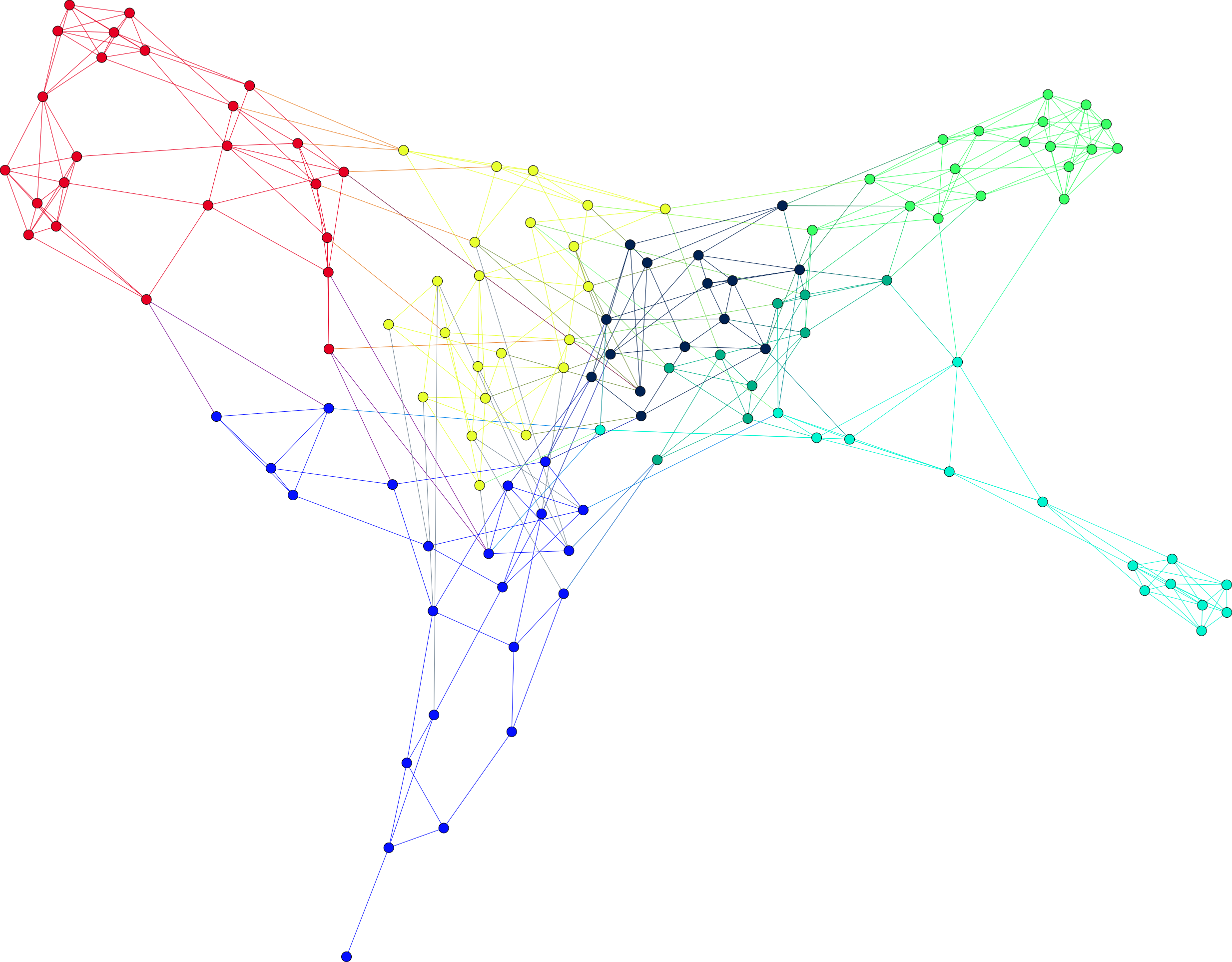
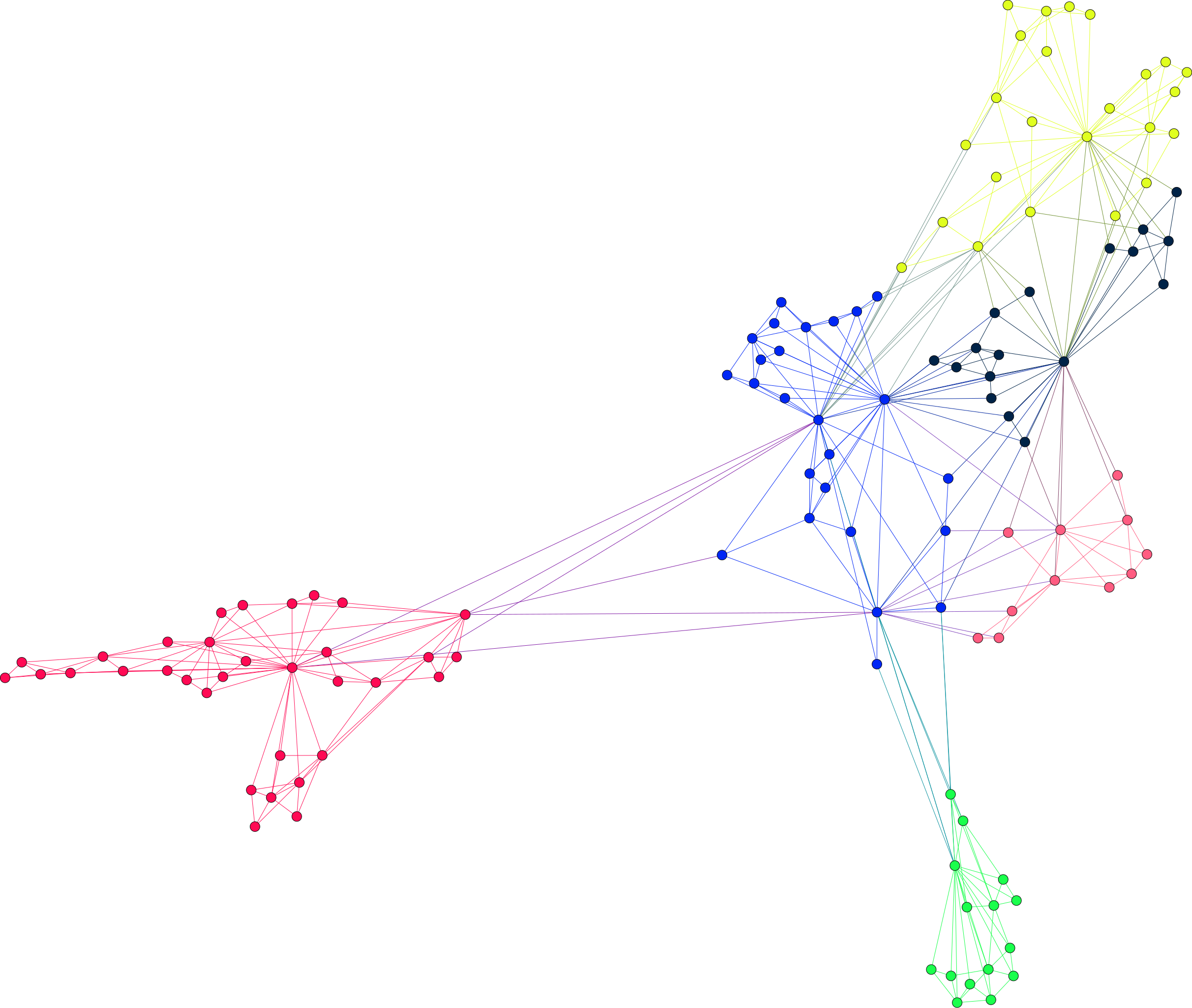
We generated the PD and PMFG networks for the above-mentioned data, the analysis of which is provided below. In the PD network, we have vertices with degrees ranging from 1 to 9 whereas in the PMFG network the degrees range from 3 to 29. Visualisations of both networks are in Figure 3.

2.5 Cliques

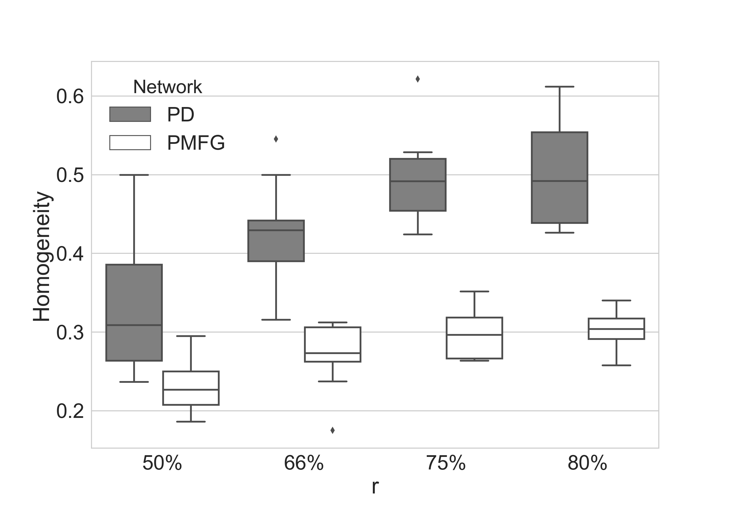
The analysis of the networks generated in the previous subsection indicates that there are 87 maximal cliques of size 3 and larger, including 52 maximal cliques of size 3, 23 of size 4, 9 of size 5, and 3 of size 6. Similarly, there are 122 maximal cliques of size 4 in PMFG network. To quantify homogeneity, $\nicefrac{{47}}{{87}}=0.54$ of the maximal cliques in the PD network consist of stocks all belonging to the same economic sector whereas this ratio is $\nicefrac{{43}}{{122}}=0.35$ for the PMFG network. We also compared the homogeneity of the maximal cliques with minimum size of 3 in the two networks on different random subsets of the stocks. To this end, we considered different proportions $r=\nicefrac{{4}}{{5}},\nicefrac{{3}}{{4}},\nicefrac{{2}}{{3}},\nicefrac{{1}}{{2}}$ of all the 125 stocks, and for each $r$, we took 10 samples of size $\lfloor r\times n\rceil$ from the stocks. We plotted the results of all samples for each $r$ and each network as shown in Figure 1, and we can see that for every $r$, the PD network has an overall larger homogeneity of maximal cliques compared with PMFG.

Figure 1: Maximal cliques homogeneity comparison of the two networks on different random subsets of proportions $r$ of all stocks

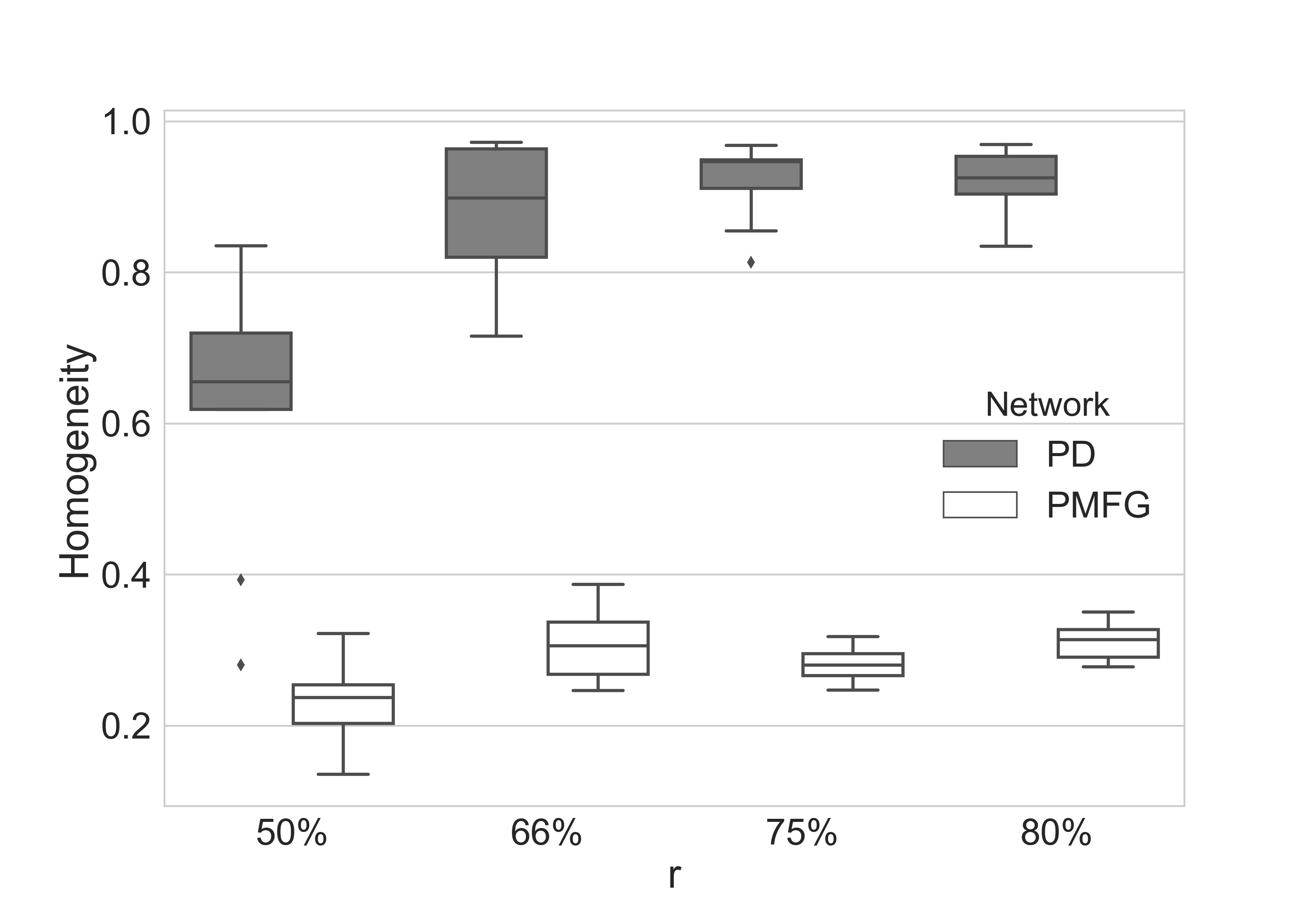
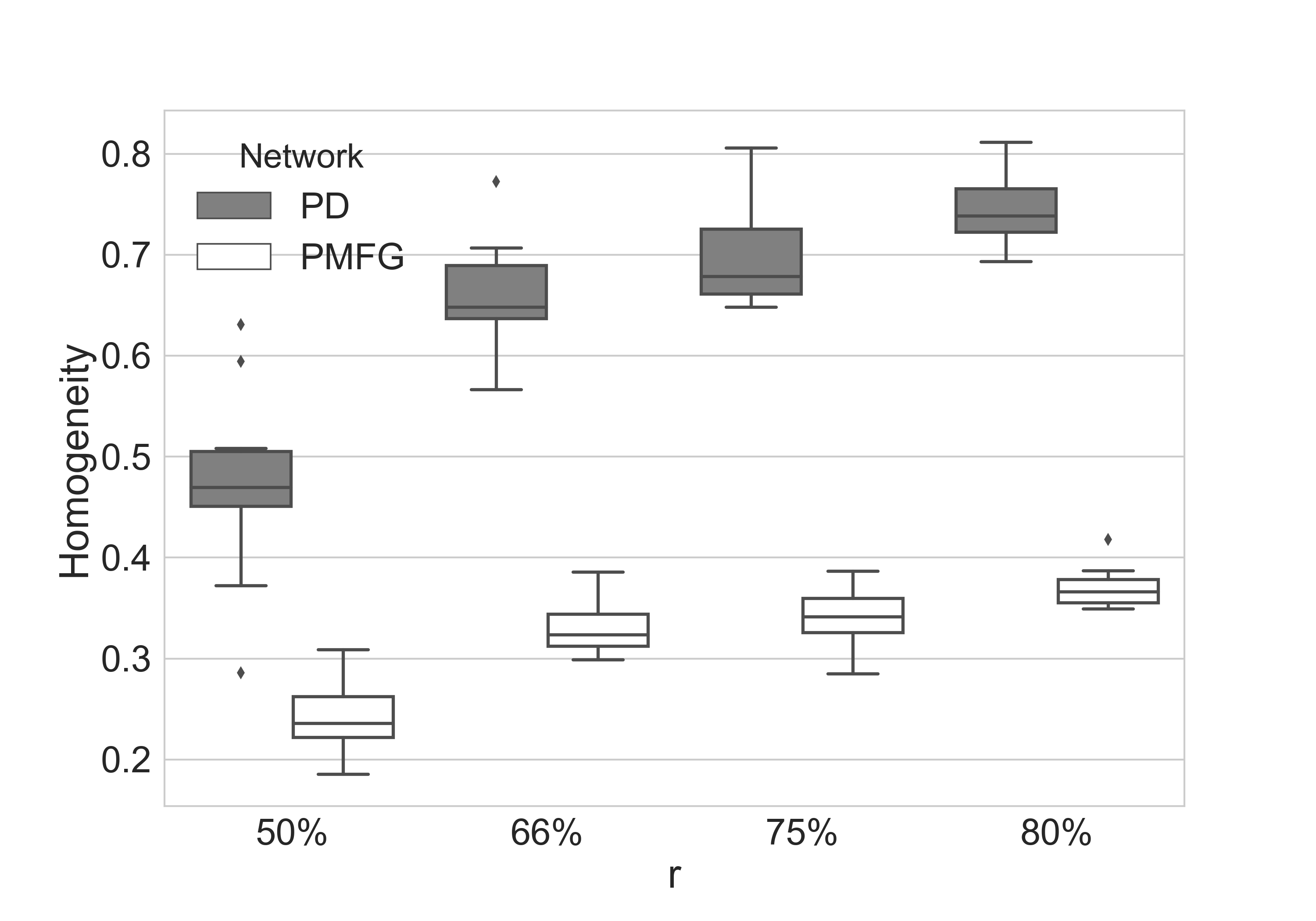
Contrasting with this, in a PMFG network, as any other planar graph, we cannot have a maximal clique with size more than 4 since such a clique cannot be embedded into a surface with genus $g=0$ without any two edges crossing. In fact, we can have at most $n-3$ maximal 4-cliques and $3n-6$ 3-cliques in any planar graph [38]. Accordingly, in another analysis, we compared the homogeneity of the 3-cliques and 4-cliques in the PD network, which are not necessarily maximal, with their counterparts in the PMFG network. There are 236 3-cliques and 101 4-cliques in the PD network, and we observe a homogeneity of $\nicefrac{{178}}{{236}}=0.75$ in the 3-cliques and $\nicefrac{{91}}{{101}}=0.90$ in the 4-cliques of it. These ratios are $\nicefrac{{152}}{{367}}=0.41$ and $\nicefrac{{43}}{{122}}=0.35$ in the PMFG network. So we can also see that all the maximal cliques in the PMFG network are 4-cliques here. As with the previous analysis, we compared the homogeneity of 3-cliques and 4-cliques of the two networks on different random subsets of the stocks, and the result is plotted on Figure 2. We can see that the comparison of 3-cliques and 4-cliques homogeneity between the two networks is even more striking than for maximal cliques.

(a) 4-cliques

(b) 3-cliques

Figure 2: 4-cliques and 3-cliques homogeneity comparison of the two networks on different random subsets of proportions $r$ of all stocks

2.6 Clusters

Using the Louvain community detection approach, following Wang and Xie[20] and Wang et al. [21], we identified clusters as shown in Tables 1 and 2. We found 7 clusters in PD and 6 in PMFG. In both tables, “Sectors” refers to the number of stocks belonging to each economic sector in the corresponding cluster, e.g. 17F denotes 17 stocks belonging to Financials sector, “Size” refers to the cluster size, “Dominant” refers to the economic sector repeated the most in the cluster, and “Percentage” refers to the proportion of the stocks belonging to the dominant sector in the cluster.

Table 1: Clusters captured in the PD network by Louvain community detection

Cluster		Sectors	Size	Dominant	Percentage
1		17F, 1RE	18	F	94%
2		13M, 7E, 4I	24	M	54%
3		10RE, 3I, 1U, 1TS	15	RE	67%
4		5HC, 2CS, 1CD, 1I	9	HC	56%
5		5CD, 5HC, 4I, 4M, 2U, 1RE, 1TS	22	CD	23%
6		8M, 5CD, 4CS, 2I, 1E, 1F, 1IT	22	M	36%
7		10CD, 2I, 1F, 1IT, 1M	15	CD	67%

Table 2: Clusters captured in the PMFG network by Louvain community detection

Cluster		Sectors	Size	Dominant	Percentage
1		10F, 5CS, 3CD, 3I, 2TS, 1HC, 1M	25	F	40%
2		19M, 8E, 5I, 1CD	33	M	58%
3		9CD, 5M, 1F, 1I, 1RE	17	CD	53%
4		9HC, 1CS, 1RE	11	HC	82%
5		8CD, 8F, 5I, 2IT, 1M	24	CD	33%
6		10RE, 3U, 2I	15	RE	67%

Nonetheless, as pointed out in Section LABEL:Louvain_subsection, Louvain community detection yields different partitions depending on the order of vertex evaluation. To mitigate the effect of different partitions corresponding to different orders of vertices on ARI, we applied the Louvain method on 100 random orders of vertices in both networks and took the average of those 100 ARIs for each method in terms of resemblance to economic sectors’ partition of stocks. This produced average ARIs of 0.31 and 0.26 for PD and PMFG networks respectively.

However, the economic sector classification is not the be-all and end-all partition of stocks. For example, every stock labelled as Real Estate in the ASX/S&P 200 data of 01/10/2018 had been put in the Financials category in the ASX/S&P 200 data of 21/03/2016, which means that the economic sector classification is subject to change, reducing the likelihood that it represents the unique correct partition. Indeed, it could also be argued that there are some significant sub-categories in other economic sectors, which would create more clusters than the number of economic sectors. To create another partition benchmark other than the economic sector classification, we used Louvain community detection on the complete graph of NMI between stocks (similarity matrix of the stocks). This computation produced only four clusters of stocks. Comparing clusters achieved by Louvain community detection in PD and PMFG networks as shown in Tables 1 and 2 with the new partition benchmark, we got ARIs of 0.40 and 0.36 respectively. Yet not much can be concluded from this comparison since the number of clusters in the benchmark partition is so different from the numbers of clusters in the two networks.

(a) Different colors referring to different clusters of Table 1

(b) Different colors referring to different clusters of Table 2

Figure 3: Clusters found in the PD (a) and PMFG (b) networks using Louvain community detection

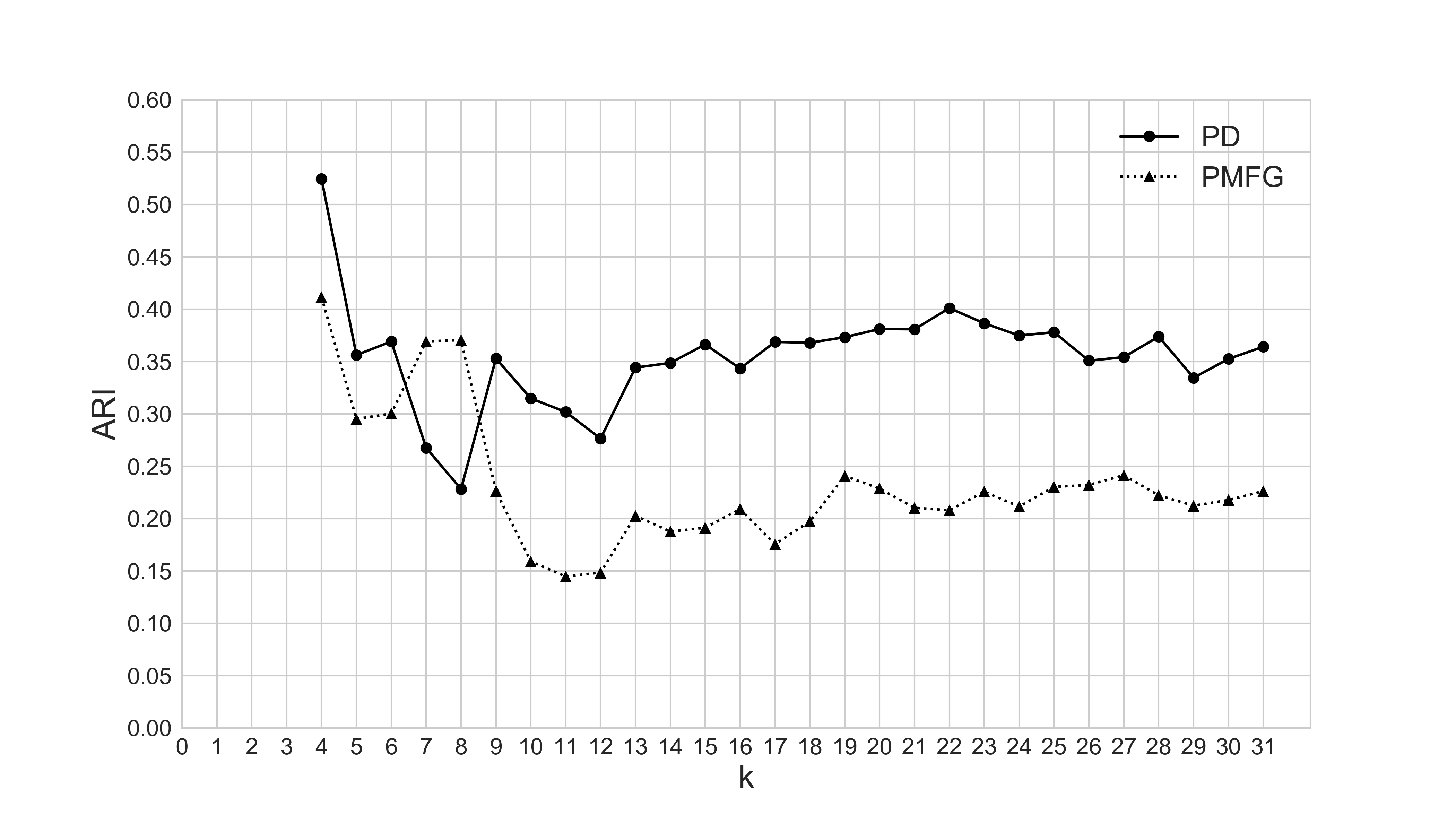
To draw a more significant comparison between the clustering behaviour of the two networks, we used NSC on the similarity matrix of the stocks and called the resulting partition $C_{\textrm{K}}$. Then we applied NSC to the PD and PMFG networks where the corresponding partitions are denoted by $C_{\textrm{PD}}$ and $C_{\textrm{PMFG}}$ respectively. For the similarity matrix to input into NSC, we used the binary adjacency matrix of the networks. In Figure 4, the Y-axis denotes the ARI of $C_{\textrm{K}}$ and $C_{\textrm{PD}}$ versus that of $C_{\textrm{K}}$ and $C_{\textrm{PMFG}}$, and the X-axis denotes $k$. Here, we regard a network to have a good ARI performance if its ARI against $C_{\textrm{K}}$ is large. It can be seen that for small values of $k$, there is not much difference in the ARI performance of the networks, for $k=7,8$, PMFG has a better ARI performance, and for $k>8$, PD consistently has a better ARI performance than PMFG. As shown in Figure 4, we restrict the number of clusters to being at least 4 because this is the least number of clusters in the application of Louvain to any of the networks or graphs under discussion, and is much smaller than the number of economic sectors.

Implementing the heuristic described in Section LABEL:NSC_subsection and ignoring the gaps between the first, second, and third sorted eigenvalues since we ignore 1 and 2 as the number of clusters, we find the largest gaps between the sorted eigenvalues for the similarity matrix are $g(\lambda_{4},\lambda_{5})=0.74$, $g(\lambda_{10},\lambda_{11})=0.35$, and $g(\lambda_{11},\lambda_{12})=0.16$. We then note that the PD network has a better ARI performance than the PMFG network for $k=4,10,11$. From another perspective, one of the points we made is that there could be some subsectors lurking in the classification of stocks by the economic sector. As we have 11 economic sectors, from this point of view, the number of clusters can be $k>11$, and for these values of $k$, PD consistently displays a better ARI performance than PMFG. It should be said that although spectral clustering does not perform well on sparse networks all the time [39, 40, 41], NSC gives a sensible result in our networks as the partitions match fairly well with the economic sector classification $C_{e}$ of the stocks as shown in Table 3. Also, the result of this table is another indicator that small values of $k$ are not valid, for the ARI of $C_{\textrm{PD}}$ and $C_{e}$ is smaller than that of $C_{\textrm{K}}$ and $C_{e}$. Besides this, the ARI of $C_{\textrm{PD}}$/$C_{\textrm{PMFG}}$ and $C_{e}$ is small for small values of $k$ compared to larger values of $k$.

Table 3: ARI of $C_{\textrm{PD}}$/$C_{\textrm{PMFG}}$/$C_{\textrm{K}}$ and $C_{e}$

k	PD	PMFG	Complete graph
5	0.195	0.0585	0.121
6	0.197	0.0921	0.124
7	0.195	0.069	0.229
8	0.236	0.1665	0.27
9	0.339	0.1557	0.352
10	0.242	0.1015	0.376
11	0.274	0.0833	0.29
12	0.279	0.0799	0.33

Figure 4: ARI performance comparison of $C_{\textrm{PD}}$ versus $C_{\textrm{PMFG}}$

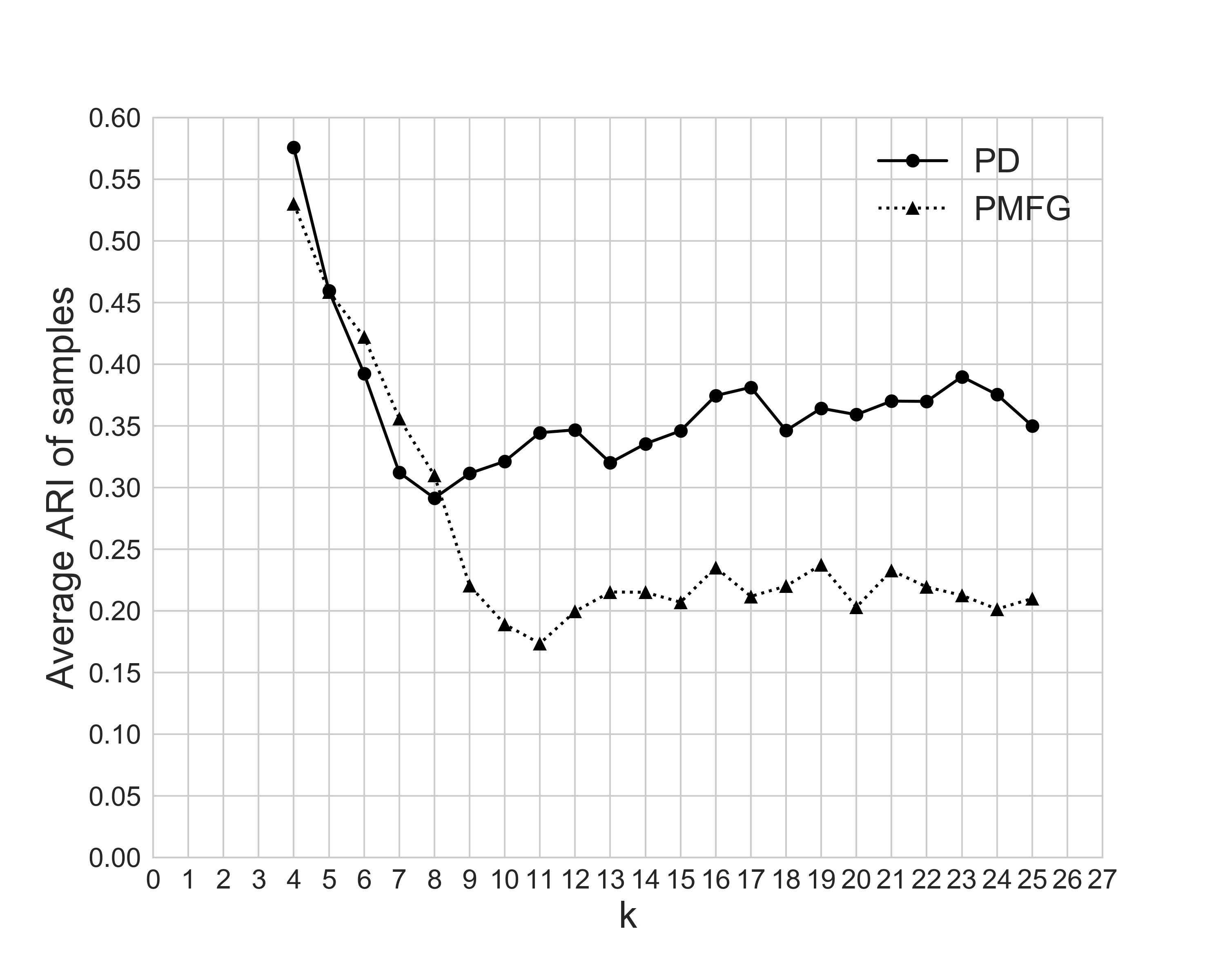
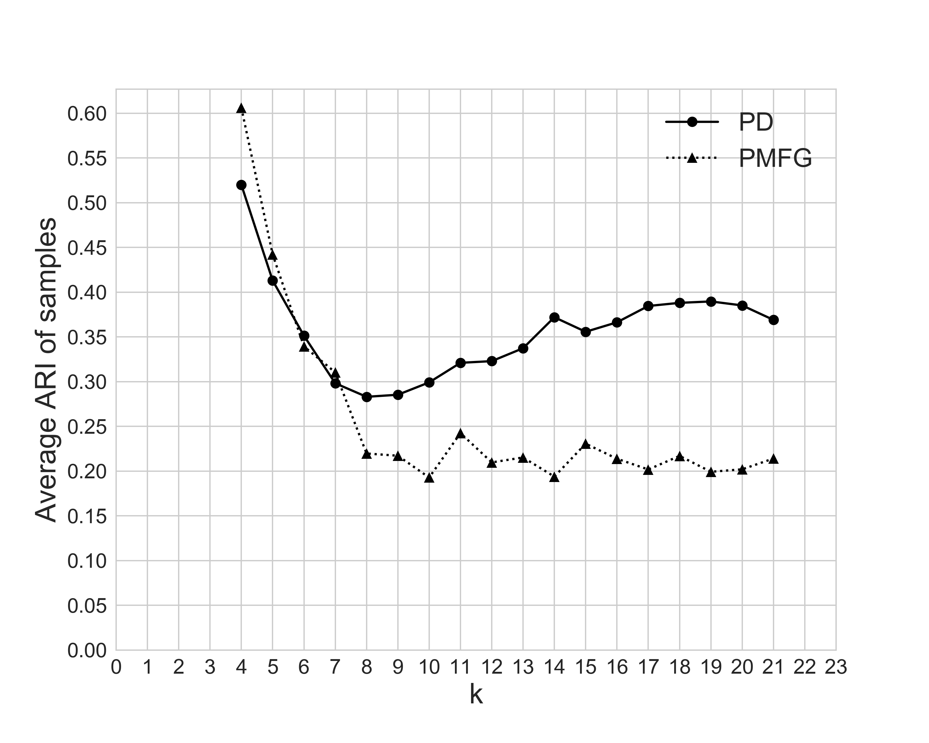
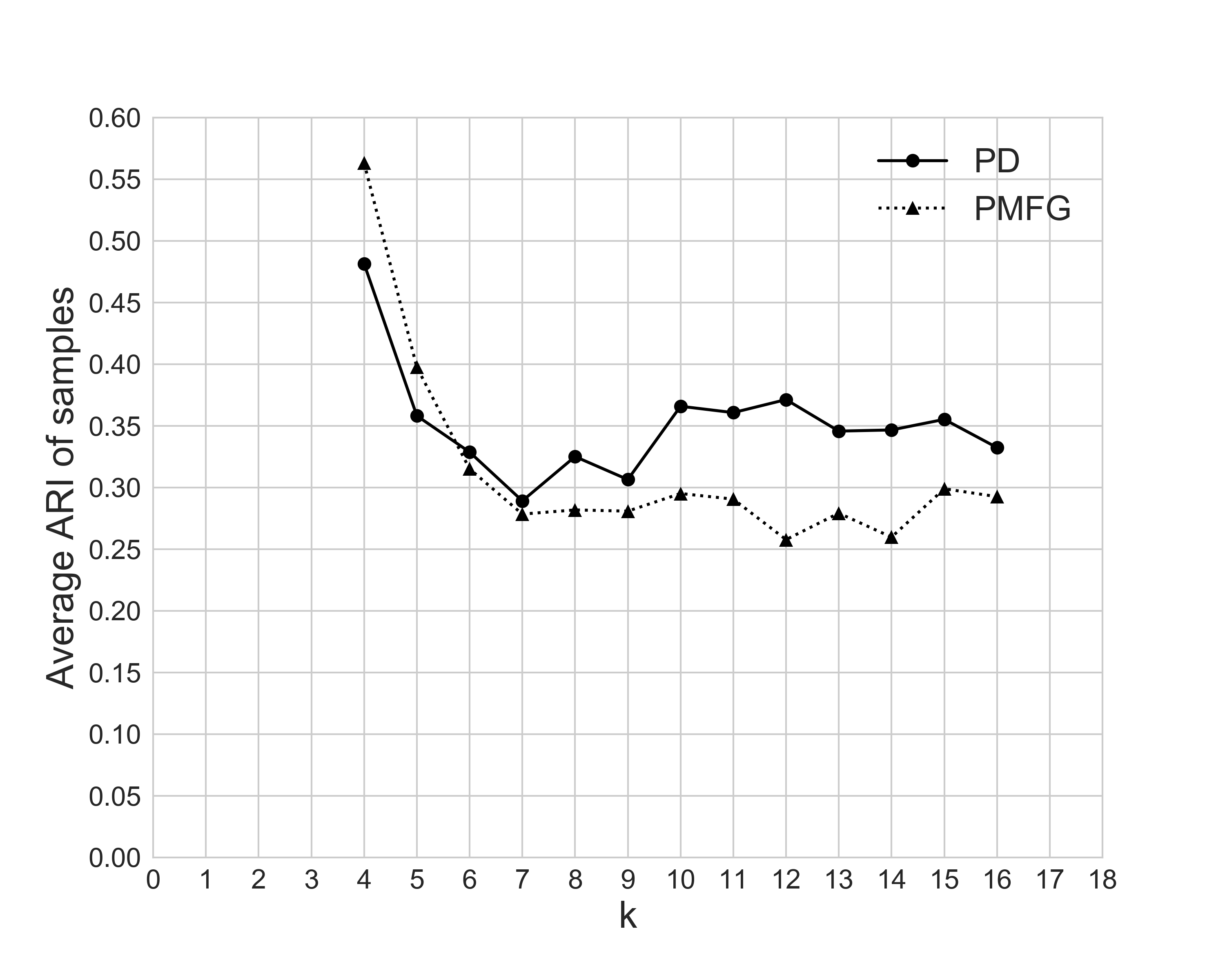
As with our analysis of the homogeneity of cliques, to test the validity of our result, we also compared the ARI performance of the two networks on different random subsets of the stocks. To this end, again, we considered different possible proportions $r=\nicefrac{{4}}{{5}},\nicefrac{{3}}{{4}},\nicefrac{{2}}{{3}},\nicefrac{{1}}{{2}}$, and for each $r$, we took 10 samples of size $\lfloor rn\rceil$ from the stocks. Then we implemented the PD and PMFG algorithms on the samples to generate the two networks and applied NSC on both networks for each sample. Denoting the partitions of PD, PMFG, and the complete similarity matrix of sample $i$ by $C_{{\rm{PD}}_{i}}$, $C_{{\rm{PMFG}}_{i}}$, and $C_{\rm{K}_{i}}$ respectively, we considered the average ARI of $C_{\rm{K}_{i}}$ and $C_{{\rm{PD}}_{i}}$ versus that of $C_{\rm{K}_{i}}$ and $C_{{\rm{PMFG}}_{i}}$ for $i=1,\ldots,10$ and plotted the results as shown in Figure 5. We can see the same pattern for every $r$; that for a large enough $k$, PD has consistently a better average ARI performance than PMFG whereas for small values of $k$, there is virtually no difference in the average ARI performance of the networks. In addition, we can see on Figure 5 that as the size of the network shrinks (for smaller values of $r$), the difference between the average ARI performance of the networks become smaller. In other words, forcing into a planar network has less effect on clustering of the stocks in smaller networks. One reason could be that there is less use of larger cliques in smaller networks; thus, the restriction of PMFG to maximal clique size of 4 becomes less important.

(a) $r=\nicefrac{{4}}{{5}}$

(b) $r=\nicefrac{{3}}{{4}}$

(c) $r=\nicefrac{{2}}{{3}}$

(d) $r=\nicefrac{{1}}{{2}}$

Figure 5: Average ARI performance of the PD and PMFG networks for different proportions $r$ of stocks

2.7 Robustness

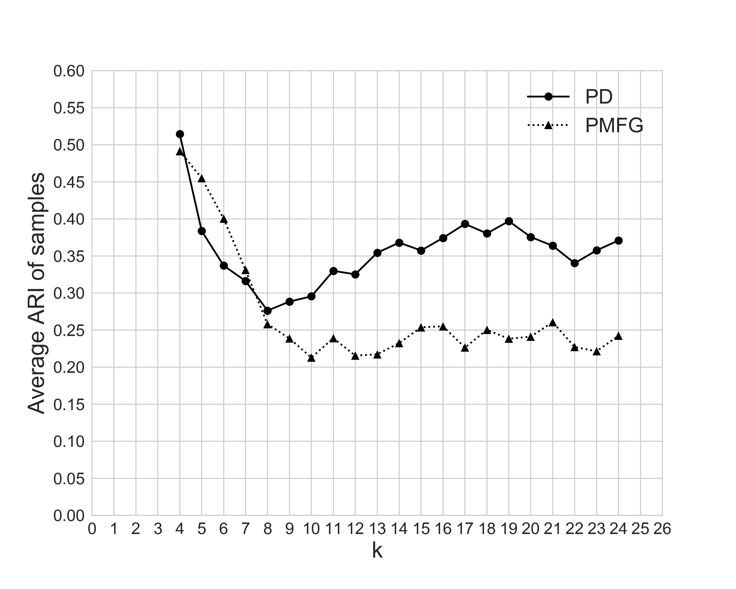
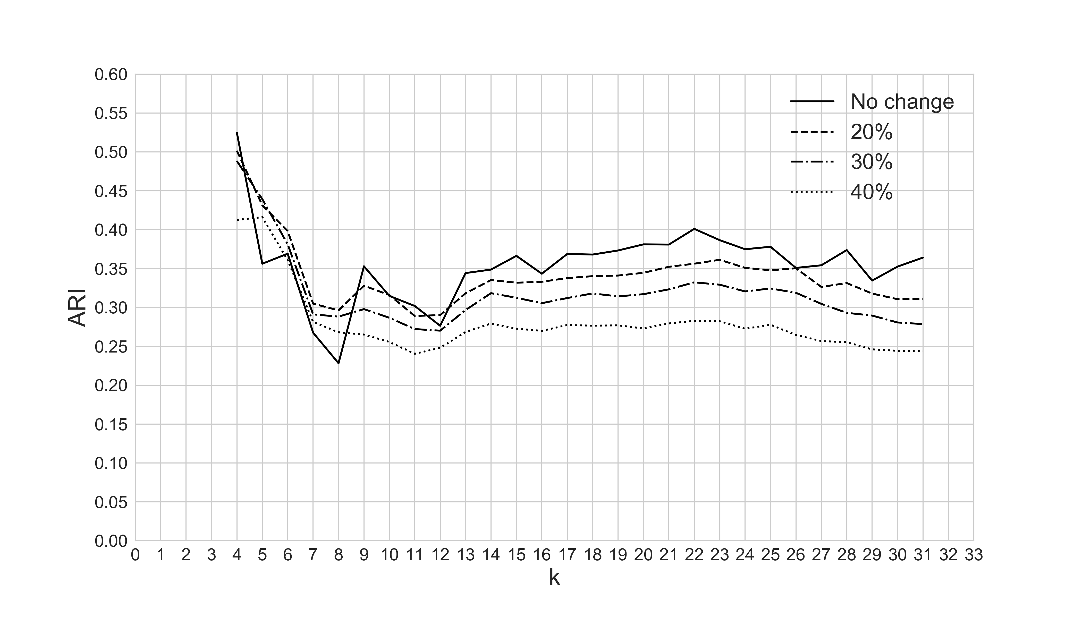
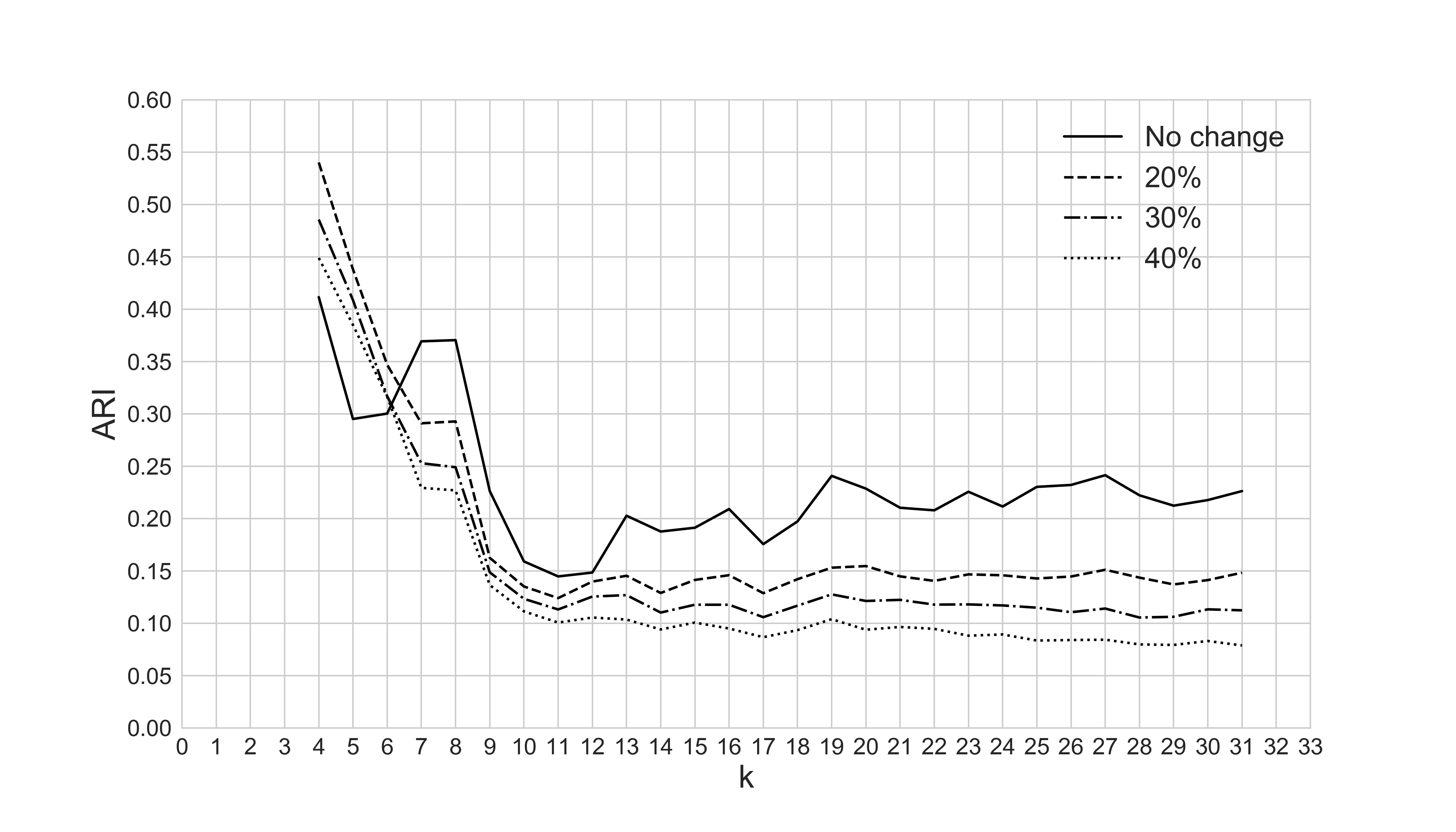
One method to investigate the robustness or stability of network is removing a subset of its vertices or edges at a certain rate [23]. On both networks, we removed 100 different samples of 20%, 30%, and 40% of the edges randomly and applied NSC on them. Then we plotted the the average ARI of $C_{\rm{K}}$ and $C_{\rm{PD}}$ and that of $C_{\rm{K}}$ and $C_{\rm{PMFG}}$ as shown in Figure 6. As expected, there is an overall decrease in ARI performance of both networks as the percentages of edge removal increases. That being said, there is an increase in the average ARI for small $k$’s ( $k\leq 8$ and $k\leq 6$ for the PD and PMFG networks respectively), which could be another indicator that small values of $k$ are not valid. Hence, PD has a better clustering behaviour that PMFG since for large values of $k$, it displays a better ARI performance.

(a) PD

(b) PMFG

Figure 6: Fluctuations in ARI for NSC of the networks for different proportions of edge removal

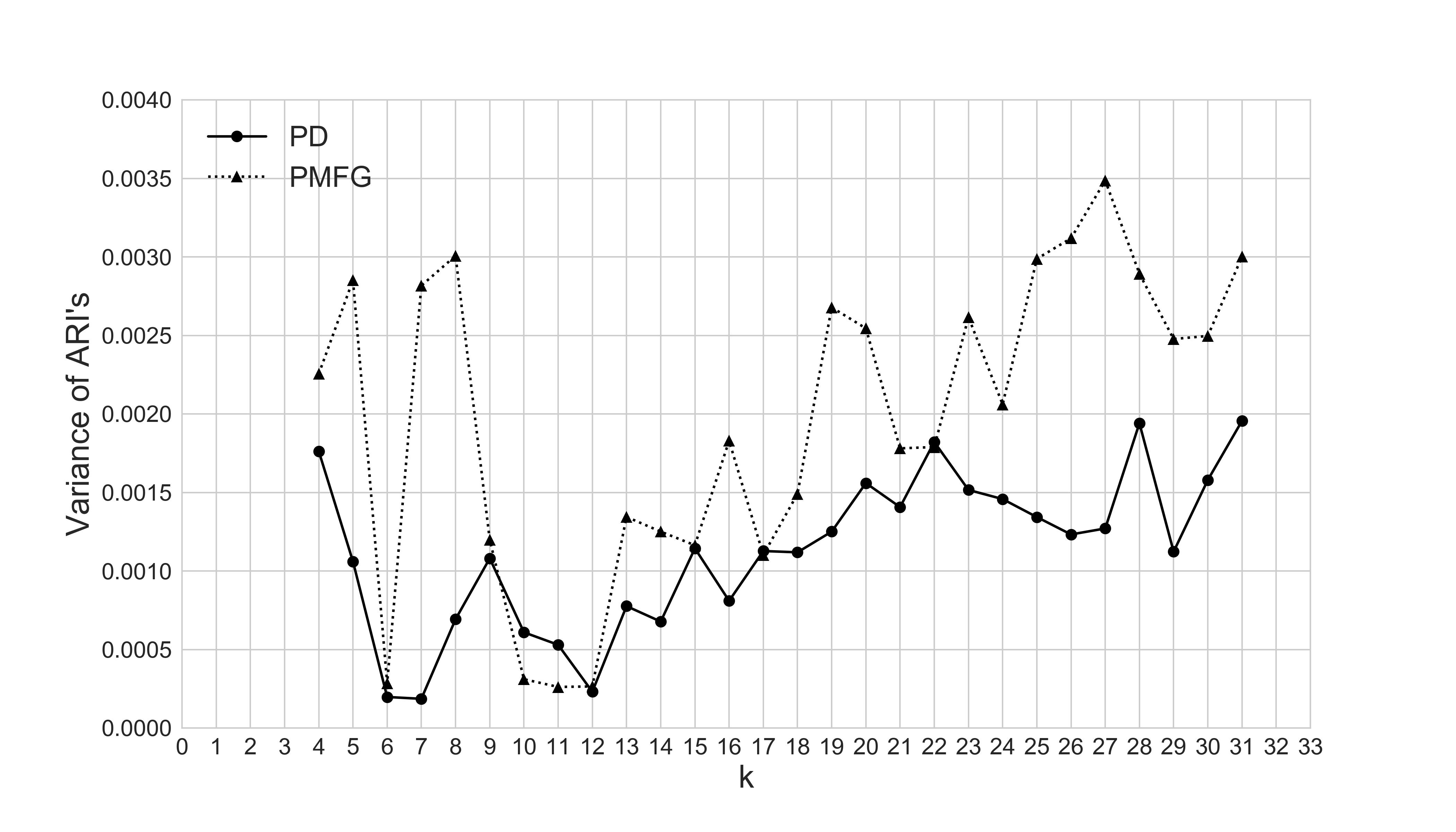
In order to see which network has more change of clusters by edge removal, we took the variance of ARIs of both networks for each $k$ in 4 states, being firstly the networks with no change, and then the networks with 20%,30%, and 40% edge removal respectively. The results are plotted on Figure 7, and we can see that for every $k$, there is either not a significant difference in the variance of the ARIs or PD has a significantly smaller variance than PMFG; thus, more robust with respect to change in clusters.

Figure 7: Robustness of the networks clusters in presence of edge removal for each $k$

3 Conclusion

We used the NMI measure to build a cross-correlation similarity matrix across stocks and applied the PD and PMFG algorithms to generate the corresponding stock-correlation networks. We showed that maximal cliques, 3-cliques, and 4-cliques had a higher homogeneity in the PD network than the PMFG network as to financial sectoral classification of the stocks. Moreover, we showed that for a realistic number of clusters in the NSC algorithm, the PD network has a better ARI performance than the PMFG network in terms of matching the clusters achieved through applying the NSC algorithm on the similarity matrix of the stocks.

It should be noted that the aforementioned results were achieved using NMI, and they are not necessarily expected using other correlation measures. Also, we used $3n-6$ edges to build the PD network for the whole purpose of comparing its performance with its PMFG counterpart. It is not clear this size of the PD network is the optimal one considering the criteria of a superior stocks-correlation network. A future topic for prospective researchers can be varying the sparsity of the PD algorithm and comparing the resulting networks. Also, other measures of correlation and dependence across stocks such as Spearman’s rank correlation coefficient could be used to build the stock-correlation network and compare that with other stock-correlation networks according to the criteria used in the literature.

References

- [1] Réka Albert and Albert-László Barabási. Statistical mechanics of complex networks. Reviews of modern physics, 74(1):47, 2002.
- [2] Réka Albert, Hawoong Jeong, and Albert-László Barabási. Internet: Diameter of the world-wide web. nature, 401(6749):130, 1999.
- [3] Albert-László Barabási, Réka Albert, and Hawoong Jeong. Scale-free characteristics of random networks: the topology of the world-wide web. Physica A: statistical mechanics and its applications, 281(1-4):69–77, 2000.
- [4] Sidney Redner. How popular is your paper? an empirical study of the citation distribution. The European Physical Journal B-Condensed Matter and Complex Systems, 4(2):131–134, 1998.
- [5] Henry Small. Co-citation in the scientific literature: A new measure of the relationship between two documents. Journal of the American Society for information Science, 24(4):265–269, 1973.
- [6] Joseph Galaskiewicz and Stanley Wasserman. Social network analysis: Concepts, methodology, and directions for the 1990s. Sociological Methods & Research, 22(1):3–22, 1993.
- [7] Stanley Wasserman and Katherine Faust. Social network analysis: Methods and applications, volume 8. Cambridge university press, 1994.
- [8] Duncan J Watts, Peter Sheridan Dodds, and Mark EJ Newman. Identity and search in social networks. science, 296(5571):1302–1305, 2002.
- [9] Mark EJ Newman, Duncan J Watts, and Steven H Strogatz. Random graph models of social networks. Proceedings of the National Academy of Sciences, 99(suppl 1):2566–2572, 2002.
- [10] Michael Boss, Helmut Elsinger, Martin Summer, and Stefan Thurner 4. Network topology of the interbank market. Quantitative finance, 4(6):677–684, 2004.
- [11] Kimmo Soramäki, Morten L Bech, Jeffrey Arnold, Robert J Glass, and Walter E Beyeler. The topology of interbank payment flows. Physica A: Statistical Mechanics and its Applications, 379(1):317–333, 2007.
- [12] Rosario N Mantegna. Hierarchical structure in financial markets. The European Physical Journal B-Condensed Matter and Complex Systems, 11(1):193–197, 1999.
- [13] Giovanni Bonanno, Guido Caldarelli, Fabrizio Lillo, and Rosario N Mantegna. Topology of correlation-based minimal spanning trees in real and model markets. Physical Review E, 68(4):046130, 2003.
- [14] Benjamin M Tabak, Thiago R Serra, and Daniel O Cajueiro. Topological properties of stock market networks: The case of brazil. Physica A: Statistical Mechanics and its Applications, 389(16):3240–3249, 2010.
- [15] Xue Guo, Hu Zhang, and Tianhai Tian. Development of stock correlation networks using mutual information and financial big data. PloS one, 13(4):e0195941, 2018.
- [16] Jukka-Pekka Onnela, Anirban Chakraborti, Kimmo Kaski, Janos Kertesz, and Antti Kanto. Asset trees and asset graphs in financial markets. Physica Scripta, 2003(T106):48, 2003.
- [17] Michele Tumminello, Tomaso Aste, Tiziana Di Matteo, and Rosario N Mantegna. A tool for filtering information in complex systems. Proceedings of the National Academy of Sciences, 102(30):10421–10426, 2005.
- [18] Michele Tumminello, Tiziana Di Matteo, Tomaso Aste, and Rosario N Mantegna. Correlation based networks of equity returns sampled at different time horizons. The European Physical Journal B, 55(2):209–217, 2007.
- [19] Dong-Ming Song, Michele Tumminello, Wei-Xing Zhou, and Rosario N Mantegna. Evolution of worldwide stock markets, correlation structure, and correlation-based graphs. Physical Review E, 84(2):026108, 2011.
- [20] Gang-Jin Wang and Chi Xie. Correlation structure and dynamics of international real estate securities markets: A network perspective. Physica A: Statistical Mechanics and its Applications, 424:176–193, 2015.
- [21] Gang-Jin Wang, Chi Xie, and Shou Chen. Multiscale correlation networks analysis of the us stock market: a wavelet analysis. Journal of Economic Interaction and Coordination, 12(3):561–594, 2017.
- [22] Vladimir Boginski, Sergiy Butenko, and Panos M Pardalos. Statistical analysis of financial networks. Computational statistics & data analysis, 48(2):431–443, 2005.
- [23] Wei-Qiang Huang, Xin-Tian Zhuang, and Shuang Yao. A network analysis of the chinese stock market. Physica A: Statistical Mechanics and its Applications, 388(14):2956–2964, 2009.
- [24] K Tse Chi, Jing Liu, and Francis CM Lau. A network perspective of the stock market. Journal of Empirical Finance, 17(4):659–667, 2010.
- [25] A Namaki, AH Shirazi, R Raei, and GR Jafari. Network analysis of a financial market based on genuine correlation and threshold method. Physica A: Statistical Mechanics and its Applications, 390(21-22):3835–3841, 2011.
- [26] Jenna Birch, Athanasios A Pantelous, and Kimmo Soramäki. Analysis of correlation based networks representing dax 30 stock price returns. Computational Economics, 47(4):501–525, 2016.
- [27] Fernando Lopes da Silva, Jan Pieter Pijn, and Peter Boeijinga. Interdependence of eeg signals: linear vs. nonlinear associations and the significance of time delays and phase shifts. Brain topography, 2(1-2):9–18, 1989.
- [28] Thomas M Cover and Joy A Thomas. Elements of information theory. John Wiley & Sons, 2012.
- [29] Claude Elwood Shannon. A mathematical theory of communication. ACM SIGMOBILE mobile computing and communications review, 5(1):3–55, 2001.
- [30] Santo Fortunato. Community detection in graphs. Physics reports, 486(3-5):75–174, 2010.
- [31] Giuseppe Buccheri, Stefano Marmi, and Rosario N Mantegna. Evolution of correlation structure of industrial indices of us equity markets. Physical Review E, 88(1):012806, 2013.
- [32] Huan Chen, Yong Mai, and Sai-Ping Li. Analysis of network clustering behavior of the chinese stock market. Physica A: Statistical Mechanics and its Applications, 414:360–367, 2014.
- [33] Vincent D Blondel, Jean-Loup Guillaume, Renaud Lambiotte, and Etienne Lefebvre. Fast unfolding of communities in large networks. Journal of statistical mechanics: theory and experiment, 2008(10):P10008, 2008.
- [34] Jianbo Shi and Jitendra Malik. Normalized cuts and image segmentation. IEEE Transactions on pattern analysis and machine intelligence, 22(8):888–905, 2000.
- [35] Lawrence Hubert and Phipps Arabie. Comparing partitions. Journal of classification, 2(1):193–218, 1985.
- [36] Ulrike Von Luxburg. A tutorial on spectral clustering. Statistics and computing, 17(4):395–416, 2007.
- [37] William M Rand. Objective criteria for the evaluation of clustering methods. Journal of the American Statistical association, 66(336):846–850, 1971.
- [38] David R Wood. On the maximum number of cliques in a graph. Graphs and Combinatorics, 23(3):337–352, 2007.
- [39] Florent Krzakala, Cristopher Moore, Elchanan Mossel, Joe Neeman, Allan Sly, Lenka Zdeborová, and Pan Zhang. Spectral redemption in clustering sparse networks. Proceedings of the National Academy of Sciences, 110(52):20935–20940, 2013.
- [40] Can M Le, Elizaveta Levina, and Roman Vershynin. Sparse random graphs: regularization and concentration of the laplacian. arXiv preprint arXiv:1502.03049, 2015.
- [41] Arash A Amini, Aiyou Chen, Peter J Bickel, Elizaveta Levina, et al. Pseudo-likelihood methods for community detection in large sparse networks. The Annals of Statistics, 41(4):2097–2122, 2013.