Mean field limits for interacting diffusions with colored noise:
phase transitions and spectral numerical methods

S.N. Gomes  [Uncaptioned image] Mathematics Institute, University of Warwick (susana.gomes@warwick.ac.uk)    G.A. Pavliotis  [Uncaptioned image] Department of Mathematics, Imperial College London (g.pavliotis@imperial.ac.uk)    U. Vaes  [Uncaptioned image] Department of Mathematics, Imperial College London (u.vaes13@imperial.ac.uk)
Abstract

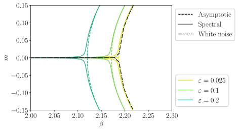
In this paper we consider systems of weakly interacting particles driven by colored noise in a bistable potential, and we study the effect of the correlation time of the noise on the bifurcation diagram for the equilibrium states. We accomplish this by solving the corresponding McKean–Vlasov equation using a Hermite spectral method, and we verify our findings using Monte Carlo simulations of the particle system. We consider both Gaussian and non-Gaussian noise processes, and for each model of the noise we also study the behavior of the system in the small correlation time regime using perturbation theory. The spectral method that we develop in this paper can be used for solving both linear and nonlinear, local and nonlocal (mean field) Fokker–Planck equations, without requiring that they have a gradient structure.

Keywords: McKean–Vlasov PDEs, Nonlocal Fokker–Planck equations, Interacting particles, Desai–Zwanzig model, Colored noise, Hermite spectral methods, Phase transitions.

AMS: 35Q70, 35Q83, 35Q84, 65N35, 65M70, 82B26,

1 Introduction

Systems of interacting particles appear in a wide variety of applications, ranging from plasma physics and galactic dynamics [5] to mathematical biology [13, 34], the social sciences [17, 37], active media [4], dynamical density functional theory (DDFT) [19, 18] and machine learning [33, 42, 45]. They can also be used in models for cooperative behavior [9], opinion formation [17], and risk management [16], and also in algorithms for global optimization [41].

In most of the existing works on the topic, the particles are assumed to be subject to thermal additive noise that is modeled as a white noise process, i.e. a mean-zero Gaussian stationary process that is delta-correlated in time. There is extensive literature studying the behavior of these systems; we mention for example works on the rigorous passage to the mean field limit [38], the long-time behavior of solutions (see [9, 44] for a case of a ferromagnetic (quartic) potential, and [20] for more general potentials), multiscale analysis [21], and phase transitions [47].

In a more realistic scenario, the system has memory and the hypothesis of Markovianity does not hold [26, 27, 28]. This memory can be modeled by using colored noise, i.e. noise with a nonzero correlation time (or, more precisely, a nonsingular autocorrelation function), which is the approach we take in this paper. For simplicity, we will assume that the noise is additive and that it can be represented by a finite-dimensional Markov process, as in the recent study [11] on mean field limits for non-Markovian interacting particles.

In this paper we will study the dynamics of a system of interacting particles of the Desai–Zwanzig type, interacting via a quadratic Curie–Weiss potential. The system of interacting particles is modeled by a system of stochastic differential equations (SDEs):

dXtidt=(V(Xti)+θ(Xti1Nj=1NXtj))+2β1ξti,i=1,,N,formulae-sequencedsuperscriptsubscript𝑋𝑡𝑖d𝑡superscript𝑉superscriptsubscript𝑋𝑡𝑖𝜃superscriptsubscript𝑋𝑡𝑖1𝑁superscriptsubscript𝑗1𝑁superscriptsubscript𝑋𝑡𝑗2superscript𝛽1superscriptsubscript𝜉𝑡𝑖𝑖1𝑁\frac{\mathrm{d}X_{t}^{i}}{\mathrm{d}t}=-\left(V^{\prime}(X_{t}^{i})+\theta\,\left(X_{t}^{i}-\frac{1}{N}\sum_{j=1}^{N}X_{t}^{j}\right)\right)+\sqrt{2\beta^{-1}}\,\xi_{t}^{i},\qquad i=1,\dotsc,N, (1.1)

where N𝑁N is the number of particles, V()𝑉V(\cdot) is a confining potential, θ𝜃\theta is the interaction strength, β𝛽\beta is the inverse temperature of the system, and ξtisuperscriptsubscript𝜉𝑡𝑖\xi_{t}^{i} are independent, identically distributed (i.i.d.) noise processes.

Before discussing the Desai–Zwanzig model with colored noise, we present a brief overview of known results [9, 44] for the white noise problem. When ξtisuperscriptsubscript𝜉𝑡𝑖\xi_{t}^{i} are white noise processes, we can pass to the mean field limit N𝑁N\to\infty in eq. 1.1 and obtain a nonlinear and nonlocal Fokker–Planck equation, known in the literature as a McKean–Vlasov equation, for the one-particle distribution function ρ(x,t)𝜌𝑥𝑡\rho(x,t):

ρt=x(V(x)ρ+θ(x𝐑xρ(x,t)dx)ρ+β1ρx).𝜌𝑡𝑥superscript𝑉𝑥𝜌𝜃𝑥subscript𝐑𝑥𝜌𝑥𝑡differential-d𝑥𝜌superscript𝛽1𝜌𝑥\mathchoice{\frac{\partial{\rho}}{\partial t}}{\partial_{t}\rho}{}{}=\mathchoice{\frac{\partial{}}{\partial x}}{\partial_{x}}{}{}\left(V^{\prime}(x)\,\rho+\theta\,\left(x-\int_{\mathbf{R}}x\,\rho(x,t)\,\mathrm{d}x\right)\,\rho+\beta^{-1}\,\mathchoice{\frac{\partial{\rho}}{\partial x}}{\partial_{x}\rho}{}{}\right). (1.2)

The McKean–Vlasov equation (1.2) is a gradient flow with respect to the quadratic Wasserstein metric for the free energy functional

[ρ]=β1𝐑ρ(x)lnρ(x)dx+𝐑V(x)ρ(x)dx+θ2𝐑𝐑F(xy)ρ(x)ρ(y)dxdy,delimited-[]𝜌superscript𝛽1subscript𝐑𝜌𝑥𝜌𝑥differential-d𝑥subscript𝐑𝑉𝑥𝜌𝑥differential-d𝑥𝜃2subscript𝐑subscript𝐑𝐹𝑥𝑦𝜌𝑥𝜌𝑦differential-d𝑥differential-d𝑦\mathcal{F}[\rho]=\beta^{-1}\int_{\mathbf{R}}\rho(x)\,\ln\rho(x)\,\mathrm{d}x+\int_{\mathbf{R}}V(x)\,\rho(x)\,\mathrm{d}x+\frac{\theta}{2}\int_{\mathbf{R}}\int_{\mathbf{R}}F(x-y)\,\rho(x)\,\rho(y)\,\mathrm{d}x\,\mathrm{d}y, (1.3)

where F(x):=x2/2assign𝐹𝑥superscript𝑥22F(x):=x^{2}/2 is the interaction potential. The long-time behavior of solutions depends on the number of local minima of the confining potential V𝑉V [47]. It follows directly from eq. 1.2 that any steady-state solution ρ(x)subscript𝜌𝑥\rho_{\infty}(x) solves, together with its first moment, the following system of equations:

x(V(x)ρ(x)+θ(xm)ρ(x)+β1ρx(x))=0,𝑥superscript𝑉𝑥subscript𝜌𝑥𝜃𝑥𝑚subscript𝜌𝑥superscript𝛽1subscript𝜌𝑥𝑥0\displaystyle\mathchoice{\frac{\partial{}}{\partial x}}{\partial_{x}}{}{}\left(V^{\prime}(x)\,\rho_{\infty}(x)+\theta\,\left(x-m\right)\,\rho_{\infty}(x)+\beta^{-1}\,\mathchoice{\frac{\partial{\rho_{\infty}}}{\partial x}}{\partial_{x}\rho_{\infty}}{}{}(x)\right)=0, (1.4a)
m=𝐑xρ(x)dx.𝑚subscript𝐑𝑥subscript𝜌𝑥differential-d𝑥\displaystyle m=\int_{\mathbf{R}}x\,\rho_{\infty}(x)\,\mathrm{d}x. (1.4b)

Since eq. 1.4a is, for m𝑚m fixed, the stationary Fokker–Planck equation associated with the overdamped Langevin dynamics in the confining potential

Veff(x;m,θ)=V(x)+θ2(xm)2,subscript𝑉eff𝑥𝑚𝜃𝑉𝑥𝜃2superscript𝑥𝑚2V_{\textrm{eff}}(x;m,\theta)=V(x)+\frac{\theta}{2}(x-m)^{2}, (1.5)

solutions can be expressed explicitly as

ρ(x;m,β,θ):=1𝒵(m,β,θ)eβVeff(x;m,θ),assignsubscript𝜌𝑥𝑚𝛽𝜃1𝒵𝑚𝛽𝜃superscripte𝛽subscript𝑉eff𝑥𝑚𝜃\rho_{\infty}(x;m,\beta,\theta):=\frac{1}{\mathcal{Z}(m,\beta,\theta)}\operatorname{e}^{-\beta V_{\textrm{eff}}(x;m,\theta)}, (1.6)

where 𝒵(m,β,θ)𝒵𝑚𝛽𝜃\mathcal{Z}(m,\beta,\theta) is the normalization constant (partition function); see [9, 20, 21] for more details. By substitution in eq. 1.4b, a scalar fixed-point problem is obtained for m𝑚m, the self-consistency equation:

m=𝐑xρ(x;m,β,θ)dx=:R(m,β,θ).m=\int_{\mathbf{R}}x\,\rho_{\infty}(x;m,\beta,\theta)\,\mathrm{d}x=:R(m,\beta,\theta). (1.7)

The stability of solutions to eq. 1.4 depends on whether they correspond to a local minimum (stable) or to a local maximum/saddle point (unstable) of the free energy functional. The free energy along the one-parameter family (1.6), with parameter m𝑚m, can be calculated explicitly [21],

[ρ(;m,β,θ)]=β1ln𝒵(m,β,θ)θ2(R(m,β,θ)m)2,delimited-[]subscript𝜌𝑚𝛽𝜃superscript𝛽1𝒵𝑚𝛽𝜃𝜃2superscript𝑅𝑚𝛽𝜃𝑚2\displaystyle\mathcal{F}[\rho_{\infty}(\,\cdot\,;m,\beta,\theta)]=-\beta^{-1}\,\ln\mathcal{Z}(m,\beta,\theta)-\frac{\theta}{2}\big{(}R(m,\beta,\theta)-m\big{)}^{2},

from which we calculate that

m[ρ(;m,β,θ)]=βθ2(R(m,β,θ)m)Var(ρ(;m,β,θ)),𝑚delimited-[]subscript𝜌𝑚𝛽𝜃𝛽superscript𝜃2𝑅𝑚𝛽𝜃𝑚Varsubscript𝜌𝑚𝛽𝜃\displaystyle\mathchoice{\frac{\partial{}}{\partial m}}{\partial_{m}}{}{}\,\mathcal{F}[\rho_{\infty}(\,\cdot\,;m,\beta,\theta)]=-\beta\theta^{2}\big{(}R(m,\beta,\theta)-m\big{)}\,\mathrm{Var}(\rho_{\infty}(\cdot\,;\,m,\beta,\theta)),

where, for a probability density ψ𝜓\psi,

Var(ψ):=𝐑(x𝐑ψ(x)dx)2ψ(x)dx.assignVar𝜓subscript𝐑superscript𝑥subscript𝐑𝜓𝑥differential-d𝑥2𝜓𝑥differential-d𝑥\mathrm{Var}(\psi):=\int_{\mathbf{R}}\left(x-\int_{\mathbf{R}}\psi(x)\,\mathrm{d}x\right)^{2}\,\psi(x)\,\mathrm{d}x.

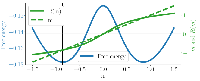
Though incomplete, this informal argument suggests that the stability of a steady-state solution can also be inferred from the slope of R(m,β,θ)m𝑅𝑚𝛽𝜃𝑚R(m,\beta,\theta)-m at the corresponding value of m𝑚m: if this slope is positive, the equilibrium is unstable, and conversely. The self-consistency map and the free energy of ρ(x;m,β,θ)subscript𝜌𝑥𝑚𝛽𝜃\rho_{\infty}(x;m,\beta,\theta), for a range of values of m𝑚m, are illustrated in fig. 1 for the bistable potential V(x)=x44x22𝑉𝑥superscript𝑥44superscript𝑥22V(x)=\frac{x^{4}}{4}-\frac{x^{2}}{2}.

Refer to caption
Figure 1: Free energy (1.3) of the one-parameter family (1.6) of probability densities that solve eq. 1.4a for some value of m𝑚m (in blue), and associated first moment R(m)𝑅𝑚R(m) (in green), for fixed θ=1𝜃1\theta=1 and β=5𝛽5\beta=5. Along the one-parameter family, m=0𝑚0m=0 is a local maximum of the free energy, and it therefore corresponds to an unstable steady state of the McKean–Vlasov equation.

It is well-known that, when V()𝑉V(\cdot) is an even potential, eq. 1.2 possesses a unique, mean-zero steady-state solution for sufficiently large temperatures (i.e., small β𝛽\beta). As the temperature decreases, this solution loses its stability and two new solutions of the self-consistency equation emerge, corresponding to a pitchfork bifurcation; see [9, 21] for details.

As mentioned above, in this paper we focus on the case where the noise processes ξtisuperscriptsubscript𝜉𝑡𝑖\xi_{t}^{i} in eq. 1.1 have a nonzero correlation time, and in particular we assume that each noise process can be represented using a (possibly multi-dimensional) SDE, in which case eq. 1.1 leads to a Markovian system of SDEs in an extended phase space. The colored noise will be modeled by either an Ornstein–Uhlenbeck process, harmonic noise [39, Example 8.2], or a non-Gaussian reversible diffusion process.

Though more realistic, the use of colored noise presents us with some difficulties. First, the introduction of an extra SDE for the noise breaks the gradient structure of the problem; while we can still pass formally to the limit N𝑁N\to\infty in eq. 1.1 and obtain a McKean–Vlasov equation for the associated one-particle distribution function, it is no longer possible to write a free energy functional, such as eq. 1.3, that is dissipated by this equation. Second, the McKean–Vlasov equation is now posed in an extended phase space, which increases the computational cost of its numerical solution via PDE methods. And third, it is no longer possible to obtain an explicit expression for the one-parameter family of (possible) stationary solutions to the mean field equation, as was possible in eq. 1.6, which renders the calculation of steady states considerably more difficult.

When the correlation time of the noise is small, the latter difficulty can be somewhat circumvented by constructing an approximate one-parameter family of solutions through appropriate asymptotic expansions in terms of the correlation time, from which steady-state solutions of the McKean–Vlasov dynamics can be extracted by solving a self-consistency equation similar to (1.7), see eq. 2.10. Outside of the small correlation time regime, however, finding the steady-states of the McKean–Vlasov equation requires a numerical method for PDEs in all but the simplest cases.

In this work, we propose a novel Hermite spectral method for the time-dependent and steady-state equations, applicable to the cases of both white and colored noise. Discretized in a basis of Hermite functions, the McKean–Vlasov equation becomes a system of ordinary differential equations with a quadratic nonlinearity originating from the interaction term. In contrast with other discretization methods for PDEs, the use of (possibly rescaled) Hermite functions for the problem under consideration leads to an efficient numerical method, first because Hermite functions have very good approximation properties in L2superscript𝐿2L^{2}, but also because all the differential operators appearing in the McKean Vlasov equation lead to sparse matrices in Hermite space, with a small bandwidth related to the polynomial degree of V𝑉V (provided that a suitable ordering of the multi-indices is employed). To solve the finite-dimensional system of equations obtained after discretization of the time-dependent equation, we employ either the Runge–Kutta 45 method (RK45) or a linear, semi-implicit time-stepping scheme.

To assess the performance of our numerical method, we compare its efficiency in the white noise case with that of the finite volume scheme developed in [8], the applicability of which depends on the existence a gradient structure of eq. 1.2. We also verify that our results agree with known analytical solutions in simple settings, and with explicit asymptotic expansions in the small correlation time regime. We then use our spectral method, together with asymptotic expansions and Monte Carlo (MC) simulations of the particle system, to construct the bifurcation diagram of the first moment of the steady-state solutions as a function of the inverse temperature.

For the reader’s convenience, we summarize here the main results of this paper:

  1. 1.

    The systematic study of the effect of colored noise, both Gaussian and non-Gaussian, on the long-time behavior of the McKean–Vlasov mean field equation, including the effect of colored noise on the structure and properties of phase transitions.

  2. 2.

    The development and analysis of a spectral numerical method for the solution of linear or nonlinear, local or nonlocal Fokker–Planck-type equations. In particular, our method does not depend on an underlying gradient structure for the PDE.

The rest of the paper is organized as follows. In Section 2, we present the models for the colored noise and we derive formally the mean field McKean–Vlasov equation associated with the interacting particle system. In Section 3, we present the numerical methods used to (a) solve the time-dependent and steady-state Fokker–Planck (or McKean–Vlasov) equations and (b) solve the finite-dimensional system of interacting diffusions (1.1). In Section 4, we study the performance of our numerical method in the small correlation time regime, and we verify numerically the convergence rates to the white noise solution in the limit where the correlation time tends to 0. In Section 5, we describe our methodology for constructing the bifurcation diagrams and we present the associated results. Section 6 is reserved for conclusions and perspectives for future work.

2 The model

We consider the following system of weakly interacting diffusions,

dXti=(V(Xti)+θ(Xti1Nj=1NXtj))dt+2β1ηtidt,1iN,formulae-sequencedsuperscriptsubscript𝑋𝑡𝑖superscript𝑉superscriptsubscript𝑋𝑡𝑖𝜃superscriptsubscript𝑋𝑡𝑖1𝑁superscriptsubscript𝑗1𝑁superscriptsubscript𝑋𝑡𝑗d𝑡2superscript𝛽1subscriptsuperscript𝜂𝑖𝑡d𝑡1𝑖𝑁\mathrm{d}X_{t}^{i}=-\left(V^{\prime}(X_{t}^{i})+\theta\left(X_{t}^{i}-\frac{1}{N}\sum_{j=1}^{N}X_{t}^{j}\right)\right)\,\mathrm{d}t+\sqrt{2\beta^{-1}}\,\eta^{i}_{t}\,\mathrm{d}t,\quad 1\leq i\leq N, (2.1)

where the noise processes ηtisubscriptsuperscript𝜂𝑖𝑡\eta^{i}_{t} are independent, mean-zero, second-order stationary processes with almost surely continuous paths and autocorrelation function K(t)𝐾𝑡K(t). In the rest of this paper, we will assume that the interaction strength θ𝜃\theta is fixed and equal to 1 and we will use the inverse temperature β1superscript𝛽1\beta^{-1} as the bifurcation parameter. We will consider two classes of models for the noise: Gaussian stationary noise processes with an exponential correlation function, and non-Gaussian noise processes that we construct by using the overdamped Langevin dynamics in a non-quadratic potential.

Gaussian noise

Stationary Gaussian processes in 𝐑nsuperscript𝐑𝑛\mathbf{R}^{n} with continuous paths and an exponential autocorrelation function are solutions to an SDE of Ornstein–Uhlenbeck type:

d𝐘ti=A𝐘tidt+2Dd𝐖ti,i=1,,N,formulae-sequencedsuperscriptsubscript𝐘𝑡𝑖𝐴superscriptsubscript𝐘𝑡𝑖d𝑡2𝐷dsuperscriptsubscript𝐖𝑡𝑖𝑖1𝑁\mathrm{d}\boldsymbol{\mathbf{Y}}_{t}^{i}=\mathit{A}\,\boldsymbol{\mathbf{Y}}_{t}^{i}\,\mathrm{d}t+\sqrt{2}\,\mathit{D}\,\mathrm{d}\boldsymbol{\mathbf{W}}_{t}^{i},\qquad i=1,\dotsc,N, (2.2)

where A,D𝐴𝐷\mathit{A},\mathit{D} are n×n𝑛𝑛n\times n matrices satisfying Kalman’s rank condition [32, Chapter 9], and 𝐖tisuperscriptsubscript𝐖𝑡𝑖\boldsymbol{\mathbf{W}}_{t}^{i}, 1in1𝑖𝑛1\leq i\leq n, are independent white noise processes in 𝐑nsuperscript𝐑𝑛\mathbf{R}^{n}. We assume here that the noise is obtained by projection as ηti=𝐘ti,𝐲ηsuperscriptsubscript𝜂𝑡𝑖superscriptsubscript𝐘𝑡𝑖subscript𝐲𝜂\eta_{t}^{i}=\left\langle{\boldsymbol{\mathbf{Y}}_{t}^{i},\boldsymbol{\mathbf{y}}_{\eta}}\right\rangle, where ,\left\langle{\cdot,\cdot}\right\rangle denotes the Euclidean inner product, for some vector 𝐲η𝐑nsubscript𝐲𝜂superscript𝐑𝑛\boldsymbol{\mathbf{y}}_{\eta}\in\mathbf{R}^{n}. Throughout this paper we will consider two particular examples, namely the scalar OU process and the harmonic noise [39, Chapter 8].

(OU)

Scalar Ornstein–Uhlenbeck process:

dηti=ηtidt+2dWti.dsuperscriptsubscript𝜂𝑡𝑖superscriptsubscript𝜂𝑡𝑖d𝑡2dsuperscriptsubscript𝑊𝑡𝑖\mathrm{d}\eta_{t}^{i}=-\eta_{t}^{i}\,\mathrm{d}t+\sqrt{2}\,\mathrm{d}W_{t}^{i}.

The associated autocorrelation function is

KOU(t)=e|t|.subscript𝐾𝑂𝑈𝑡superscript𝑒𝑡K_{OU}(t)=e^{-|t|}.
(H)

Harmonic noise:

A=(011γ),D=(000γ),𝐲η=(10).formulae-sequence𝐴matrix011𝛾formulae-sequence𝐷matrix000𝛾subscript𝐲𝜂matrix10\mathit{A}=\begin{pmatrix}0&1\\ -1&-\gamma\end{pmatrix},\quad\mathit{D}=\begin{pmatrix}0&0\\ 0&\sqrt{\gamma}\end{pmatrix},\quad\boldsymbol{\mathbf{y}}_{\eta}=\begin{pmatrix}1\\ 0\end{pmatrix}.

In this case the noise is the solution to the Langevin equation, with the first and second components of 𝐘𝐘\boldsymbol{\mathbf{Y}} corresponding to the position and velocity, respectively. Throughout this paper we will assume γ=1𝛾1\gamma=1 for simplicity. The associated autocorrelation function of ηisuperscript𝜂𝑖\eta^{i} is given by

KH(t)=e|t|2(cos(32t)+33sin(32t)).subscript𝐾𝐻𝑡superscript𝑒𝑡232𝑡3332𝑡K_{H}(t)=e^{-\frac{|t|}{2}}\left(\cos\left(\frac{\sqrt{3}}{2}t\right)+\frac{\sqrt{3}}{3}\sin\left(\frac{\sqrt{3}}{2}t\right)\right).

Non-Gaussian noise

In this case, instead of eq. 2.2 we consider

dηti=Vη(ηti)dt+2dWti,dsuperscriptsubscript𝜂𝑡𝑖superscriptsubscript𝑉𝜂superscriptsubscript𝜂𝑡𝑖d𝑡2dsuperscriptsubscript𝑊𝑡𝑖\mathrm{d}\eta_{t}^{i}=-V_{\eta}^{\prime}(\eta_{t}^{i})\,\mathrm{d}t+\sqrt{2}\,\mathrm{d}{W}_{t}^{i},

where now Vηsubscript𝑉𝜂V_{\eta} is a smooth non-quadratic confining potential satisfying the mean-zero condition:

𝐑ηeVη(η)dη=0.subscript𝐑𝜂superscriptesubscript𝑉𝜂𝜂d𝜂0\int_{\mathbf{R}}\eta\,\operatorname{e}^{-V_{\eta}(\eta)}\,\mathrm{d}\eta=0. (2.3)

We consider the following choices for Vηsubscript𝑉𝜂V_{\eta}:

(B)

The bistable potential Vη(η)=η4/4η2/2subscript𝑉𝜂𝜂superscript𝜂44superscript𝜂22V_{\eta}(\eta)=\eta^{4}/4-\eta^{2}/2.

(NS)

The shifted tilted bistable potential

Vη(η)=(ηα)44(ηα)22+(ηα),subscript𝑉𝜂𝜂superscript𝜂𝛼44superscript𝜂𝛼22𝜂𝛼V_{\eta}(\eta)=\frac{{(\eta-\alpha)}^{4}}{4}-\frac{{(\eta-\alpha)}^{2}}{2}+(\eta-\alpha), (2.4)

with the constant α0.885𝛼0.885\alpha\approx 0.885 such that eq. 2.3 is satisfied.

Remark 2.1.

For the two Gaussian noise processes we consider, it would have been equivalent (by a change of variables) to include the inverse temperature β𝛽\beta in the noise equation eq. 2.2 rather than in eq. 2.1. This is not the case for non-Gaussian noise processes, for which including the temperature in the noise equation leads to an effective diffusion coefficient, in the limit as the correlation time tends to 0, with a nonlinear dependence on β𝛽\beta.

2.1 Mean field limit

For weakly interacting diffusions, the derivation of the mean field McKean–Vlasov PDE is a standard, well-known result [9, 44, 38]. When ξtisuperscriptsubscript𝜉𝑡𝑖\xi_{t}^{i} in (1.1) are colored noise processes, it is also possible to pass to the mean field limit N𝑁N\to\infty in eq. 1.1 and to obtain a McKean–Vlasov equation for the one-particle distribution function ρ(x,𝐲,t)𝜌𝑥𝐲𝑡\rho(x,\boldsymbol{\mathbf{y}},t):

ρt=x(Vρ+θ(xm(t))ρ2β1𝐲i,𝐲ηρ)+𝐲ρ,𝜌𝑡𝑥superscript𝑉𝜌𝜃𝑥𝑚𝑡𝜌2superscript𝛽1subscript𝐲𝑖subscript𝐲𝜂𝜌superscriptsubscript𝐲𝜌\mathchoice{\frac{\partial{\rho}}{\partial t}}{\partial_{t}\rho}{}{}=\mathchoice{\frac{\partial{}}{\partial x}}{\partial_{x}}{}{}\left(V^{\prime}\rho+\theta\,(x-m(t))\,\rho-\sqrt{2\beta^{-1}}\,\left\langle{\boldsymbol{\mathbf{y}}_{i},\boldsymbol{\mathbf{y}}_{\eta}}\right\rangle\,\rho\right)+\mathcal{L}_{\boldsymbol{\mathbf{y}}}^{*}\rho, (2.5a)
with the dynamic constraint
m(t)=𝐑𝐑nxρ(x,𝐲,t)d𝐲dx.𝑚𝑡subscript𝐑subscriptsuperscript𝐑𝑛𝑥𝜌𝑥𝐲𝑡differential-d𝐲differential-d𝑥m(t)=\int_{\mathbf{R}}\int_{\mathbf{R}^{n}}x\,\rho(x,\boldsymbol{\mathbf{y}},t)\,\mathrm{d}\boldsymbol{\mathbf{y}}\,\mathrm{d}x. (2.5b)

Here 𝐲𝐲\boldsymbol{\mathbf{y}} are the noise variables, denoted by (η,λ)𝜂𝜆(\eta,\lambda) in the case of harmonic noise and just η𝜂\eta otherwise, and

𝐲ρ={η(ηρ+ηρ),for scalar OU noise,λ(λρ+λρ)+(ηλρληρ),for harmonic noise,η(Vηρ+ηρ),for non-Gaussian noise.superscriptsubscript𝐲𝜌casessubscript𝜂𝜂𝜌subscript𝜂𝜌for scalar OU noise,subscript𝜆𝜆𝜌subscript𝜆𝜌𝜂subscript𝜆𝜌𝜆subscript𝜂𝜌for harmonic noise,subscript𝜂superscriptsubscript𝑉𝜂𝜌subscript𝜂𝜌for non-Gaussian noise\mathcal{L}_{\boldsymbol{\mathbf{y}}}^{*}\rho=\begin{cases}\mathchoice{\frac{\partial{}}{\partial{\eta}}}{\partial_{\eta}}{}{}\left(\eta\,\rho+\mathchoice{\frac{\partial{\rho}}{\partial{\eta}}}{\partial_{\eta}\rho}{}{}\right),&\textrm{for scalar OU noise,}\\ \mathchoice{\frac{\partial{}}{\partial{\lambda}}}{\partial_{\lambda}}{}{}\left(\lambda\,\rho+\mathchoice{\frac{\partial{\rho}}{\partial{\lambda}}}{\partial_{\lambda}\rho}{}{}\right)+\left(\eta\,\mathchoice{\frac{\partial{\rho}}{\partial{\lambda}}}{\partial_{\lambda}\rho}{}{}-\lambda\,\mathchoice{\frac{\partial{\rho}}{\partial{\eta}}}{\partial_{\eta}\rho}{}{}\right),&\textrm{for harmonic noise,}\\ \mathchoice{\frac{\partial{}}{\partial{\eta}}}{\partial_{\eta}}{}{}\left(V_{\eta}^{\prime}\,\rho+\mathchoice{\frac{\partial{}}{\partial{\eta}}}{\partial_{\eta}}{}{}\rho\right),&\textrm{for non-Gaussian noise}.\end{cases}

A formal derivation of the mean field limit is presented in [49], and this derivation can be justified rigorously using the results in [12, 36].

The main goal of this paper is the study of the effect of colored noise on the structure of the bifurcation diagram for the McKean–Vlasov equation with colored noise, eqs. 2.5a and 2.5b. In other words, we want to gain insight into the number of solutions to the following stationary PDE and associated constraint (self-consistency equation):

x(V(x)ρ+θ(xm)ρ2β1𝐲i,𝐲ηρ)+𝐲ρ=0,𝑥superscript𝑉𝑥𝜌𝜃𝑥𝑚𝜌2superscript𝛽1subscript𝐲𝑖subscript𝐲𝜂𝜌superscriptsubscript𝐲𝜌0\mathchoice{\frac{\partial{}}{\partial x}}{\partial_{x}}{}{}\left(V^{\prime}(x)\,\rho+\theta\,(x-m)\,\rho-\sqrt{2\beta^{-1}}\,\left\langle{\boldsymbol{\mathbf{y}}_{i},\boldsymbol{\mathbf{y}}_{\eta}}\right\rangle\,\rho\right)+\mathcal{L}_{\boldsymbol{\mathbf{y}}}^{*}\rho=0, (2.6a)
m=𝐑𝐑nxρ(x,𝐲)d𝐲dx.𝑚subscript𝐑subscriptsuperscript𝐑𝑛𝑥𝜌𝑥𝐲differential-d𝐲differential-d𝑥m=\int_{\mathbf{R}}\int_{\mathbf{R}^{n}}x\,\rho(x,\boldsymbol{\mathbf{y}})\,\mathrm{d}\boldsymbol{\mathbf{y}}\,\mathrm{d}x. (2.6b)

Although there still exists, for fixed β𝛽\beta and fixed θ𝜃\theta, a one-parameter family of solutions to (2.6a) (with parameter m𝑚m), which we will denote by {ρ(x,𝐲;m,β,θ)}m𝐑subscriptsubscript𝜌𝑥𝐲𝑚𝛽𝜃𝑚𝐑\{\rho_{\infty}(x,\boldsymbol{\mathbf{y}};m,\beta,\theta)\}_{m\in\mathbf{R}}, no closed form is available for these solutions. This is because the detailed balance condition no longer holds in the presence of colored noise, i.e. the probability flux at equilibrium does not vanish. Here, by probability flux, we mean the argument of the divergence in the Fokker–Planck operator; see [39, Section 4.6].

2.2 The white noise limit

To study the limit of small correlation time, it will be convenient to rescale the noise as

ηtiζηt/ε2i/ε,subscriptsuperscript𝜂𝑖𝑡𝜁superscriptsubscript𝜂𝑡superscript𝜀2𝑖𝜀\eta^{i}_{t}\rightarrow\zeta\,\eta_{t/\varepsilon^{2}}^{i}/\varepsilon,

where ε𝜀\varepsilon is a time scaling parameter, and ζ𝜁\zeta is a model-dependent parameter ensuring that the autocorrelation function of the rescaled noise, given by ζ2K(t/ε2)/ε2superscript𝜁2𝐾𝑡superscript𝜀2superscript𝜀2\zeta^{2}\,K(t/\varepsilon^{2})/\varepsilon^{2}, satisfies

0ζ2K(t/ε2)/ε2dt=0ζ2K(t)dt=12.superscriptsubscript0superscript𝜁2𝐾𝑡superscript𝜀2superscript𝜀2differential-d𝑡superscriptsubscript0superscript𝜁2𝐾𝑡differential-d𝑡12\int_{0}^{\infty}\zeta^{2}K(t/\varepsilon^{2})/\varepsilon^{2}\,\mathrm{d}t=\int_{0}^{\infty}\zeta^{2}K(t)\,\mathrm{d}t=\frac{1}{2}.

Then the autocorrelation of the noise converges to a Dirac delta when ε0𝜀0\varepsilon\to 0, and it can be shown that, in this limit, the solution of eq. 2.1 converges to that of

dXti=(V(Xti)θ(Xti1Nj=0NXtj))dt+2β1dWti,i=1,N,formulae-sequencedsuperscriptsubscript𝑋𝑡𝑖superscript𝑉superscriptsubscript𝑋𝑡𝑖𝜃superscriptsubscript𝑋𝑡𝑖1𝑁superscriptsubscript𝑗0𝑁superscriptsubscript𝑋𝑡𝑗d𝑡2superscript𝛽1dsubscriptsuperscript𝑊𝑖𝑡𝑖1𝑁\mathrm{d}X_{t}^{i}=\left(-V^{\prime}(X_{t}^{i})-\theta\left(X_{t}^{i}-\frac{1}{N}\sum_{j=0}^{N}X_{t}^{j}\right)\right)\,\mathrm{d}t+\sqrt{2\beta^{-1}}\,\mathrm{d}W^{i}_{t},\quad i=1,\dotsc N,

where Wisuperscript𝑊𝑖W^{i}, i=1,N𝑖1𝑁i=1,\dotsc N, are independent Wiener processes; see [6] and [40, Chapter 11]. While not strictly necessary, including the parameter ζ𝜁\zeta is convenient to obtain simpler formulas. The value of ζ𝜁\zeta for each of the noise models considered in this paper is presented in table 1. For the models B and NS, ζ𝜁\zeta was calculated numerically and rounded to three significant figures in this table.

Table 1: Value of ζ𝜁\zeta
Model OU H B NS
ζ𝜁\zeta 1/2121/\sqrt{2} 1/2121/\sqrt{2} 0.6240.6240.624 0.9440.9440.944

In view of the convergence of the solution of the finite-dimensional particle system when ε0𝜀0\varepsilon\to 0, we expect that also the x𝑥x-marginals of the steady-state solutions to the McKean–Vlasov equation with colored noise, obtained by solving eqs. 2.6a and 2.6b, should converge to their white-noise counterparts as ε0𝜀0\varepsilon\to 0. It turns out that this is the case and, using asymptotic techniques from [26], it is possible to approximate the solutions ρ(x,𝐲;m,β,θ)subscript𝜌𝑥𝐲𝑚𝛽𝜃\rho_{\infty}(x,\boldsymbol{\mathbf{y}};m,\beta,\theta) to eq. 2.6a by a power series expansion in ε𝜀\varepsilon; using a superscript to emphasize the dependence on ε𝜀\varepsilon,

ρε(x,𝐲;m,β,θ)=p0(x,𝐲;m,β,θ)+εp1(x,𝐲;m,β,θ)+ε2p2(x,𝐲;m,β,θ)+,superscriptsubscript𝜌𝜀𝑥𝐲𝑚𝛽𝜃subscript𝑝0𝑥𝐲𝑚𝛽𝜃𝜀subscript𝑝1𝑥𝐲𝑚𝛽𝜃superscript𝜀2subscript𝑝2𝑥𝐲𝑚𝛽𝜃\rho_{\infty}^{\varepsilon}(x,\boldsymbol{\mathbf{y}};m,\beta,\theta)=p_{0}(x,\boldsymbol{\mathbf{y}};m,\beta,\theta)+\varepsilon\,p_{1}(x,\boldsymbol{\mathbf{y}};m,\beta,\theta)+\varepsilon^{2}\,p_{2}(x,\boldsymbol{\mathbf{y}};m,\beta,\theta)+\dotsb, (2.7)

From eq. 2.7, we obtain a power series expansion for the x𝑥x-marginal by integrating out the noise variable:

ρε(x;m,β,θ)subscriptsuperscript𝜌𝜀𝑥𝑚𝛽𝜃\displaystyle\rho^{\varepsilon}_{\infty}(x;m,\beta,\theta) =𝐑nρε(x,𝐲;m,β,θ)d𝐲absentsubscriptsuperscript𝐑𝑛subscriptsuperscript𝜌𝜀𝑥𝐲𝑚𝛽𝜃differential-d𝐲\displaystyle=\int_{\mathbf{R}^{n}}\rho^{\varepsilon}_{\infty}(x,\boldsymbol{\mathbf{y}};m,\beta,\theta)\,\mathrm{d}\boldsymbol{\mathbf{y}} (2.8)
=:ρ(x;m,β,θ)+εp1(x;m,β,θ)+ε2p2(x;m,β,θ)+,\displaystyle=:\rho_{\infty}(x;m,\beta,\theta)+\varepsilon\,p_{1}(x;m,\beta,\theta)+\varepsilon^{2}\,p_{2}(x;m,\beta,\theta)+\dotsb,

The methodology to obtain expressions for the terms works by substituting eq. 2.7 in eq. 2.6a and grouping the terms in powers of ε𝜀\varepsilon in the resulting equation. This leads to a sequence of equations that can be studied using standard techniques. Details of the analysis leading to an explicit expression of the first nonzero correction in (2.8) can be found in [26, Section 8] for the particular case of the OU noise, and in [49] for the other noise models we consider.

The order of the first nonzero correction in this expansion depends on the model: it is equal to 1 for model NS, to 2 for models OU and B, and to 4 for model H. In all cases, the first nontrivial term in the series expansion (2.8) can be calculated explicitly (possibly up to constant coefficients that have to be calculated numerically). For scalar Ornstein–Uhlenbeck noise, for example, we have, omitting the dependence of Veffsubscript𝑉effV_{\textrm{eff}} (the effective potential defined in eq. 1.5) on m𝑚m and θ𝜃\theta for notational convenience,

ρε(x;m,β,θ)=ρ(x;m,β,θ)[1+ε2(COUβ2(Veff(x))2+Veff′′(x))]+𝒪(ε4)subscriptsuperscript𝜌𝜀𝑥𝑚𝛽𝜃subscript𝜌𝑥𝑚𝛽𝜃delimited-[]1superscript𝜀2subscript𝐶𝑂𝑈𝛽2superscriptsuperscriptsubscript𝑉eff𝑥2superscriptsubscript𝑉eff′′𝑥𝒪superscript𝜀4\displaystyle\rho^{\varepsilon}_{\infty}(x;m,\beta,\theta)=\rho_{\infty}(x;m,\beta,\theta)\left[1+\varepsilon^{2}\left(C_{OU}-\frac{\beta}{2}\left(V_{\textrm{eff}}^{\prime}{\left(x\right)}\right)^{2}+V_{\textrm{eff}}^{\prime\prime}{\left(x\right)}\right)\right]+\mathcal{O}(\varepsilon^{4}) (2.9)

Here COUsubscript𝐶𝑂𝑈C_{OU} is a constant such that the correction integrates to 00. Similar expressions can be obtained for the other models; see [49].

Taking into account only the first nontrivial correction, the order of which we denote by δ𝛿\delta, the steady-state solutions to the McKean–Vlasov equation with colored noise can be approximated by solving the approximate self-consistency equation

m𝑚\displaystyle m =R0(m,β,θ)+εδRδ(m,β,θ)absentsubscript𝑅0𝑚𝛽𝜃superscript𝜀𝛿subscript𝑅𝛿𝑚𝛽𝜃\displaystyle=R_{0}(m,\beta,\theta)+\varepsilon^{\delta}\,R_{\delta}(m,\beta,\theta)
:=𝐑xρ(x;m,β,θ)dx+εδ𝐑xpδ(x;m,β,θ)dxassignabsentsubscript𝐑𝑥subscript𝜌𝑥𝑚𝛽𝜃differential-d𝑥superscript𝜀𝛿subscript𝐑𝑥subscript𝑝𝛿𝑥𝑚𝛽𝜃differential-d𝑥\displaystyle:=\int_{\mathbf{R}}x\,\rho_{\infty}(x;m,\beta,\theta)\,\mathrm{d}x+\varepsilon^{\delta}\int_{\mathbf{R}}x\,p_{\delta}(x;m,\beta,\theta)\,\mathrm{d}x (2.10)
R(m,β):=𝐑xρε(x;m,β,θ)dx.absent𝑅𝑚𝛽assignsubscript𝐑𝑥subscriptsuperscript𝜌𝜀𝑥𝑚𝛽𝜃differential-d𝑥\displaystyle\approx R(m,\beta):=\int_{\mathbf{R}}x\,\rho^{\varepsilon}_{\infty}(x;m,\beta,\theta)\,\mathrm{d}x.

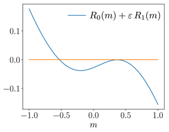
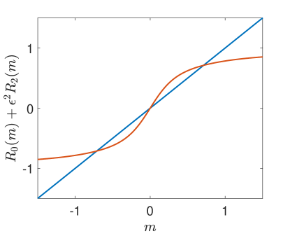
We show in fig. 2 that the equation R0(m,β,θ)+ε2R2(m,β,θ)=msubscript𝑅0𝑚𝛽𝜃superscript𝜀2subscript𝑅2𝑚𝛽𝜃𝑚R_{0}(m,\beta,\theta)+\varepsilon^{2}R_{2}(m,\beta,\theta)=m, for fixed β=10𝛽10\beta=10, θ=1𝜃1\theta=1 and ε=0.1𝜀0.1\varepsilon=0.1, admits three solutions in the case of OU noise, similarly to the case of white noise. This figure was generated using the asymptotic expansion (2.9).
Refer to caption
Figure 2: Truncated asymptotic expansion of the self-consistency map, R0+ε2R2subscript𝑅0superscript𝜀2subscript𝑅2R_{0}+\varepsilon^{2}\,R_{2}, as a function of m𝑚m (red line) compared to y=m𝑦𝑚y=m (blue line) for the scalar Ornstein–Uhlenbeck noise, with β=10,θ=1,ε=0.1formulae-sequence𝛽10formulae-sequence𝜃1𝜀0.1\beta=10,\,\theta=1,\,\varepsilon=0.1.

3 The numerical method

In this section, we describe the spectral numerical method that we will use in order to solve the time-dependent McKean–Vlasov equation, eqs. 2.5a and 2.5b, as well as the steady-state equation, eqs. 2.6a and 2.6b. Before looking at colored noise, we consider the case of white noise, for which our method can be tested against the results in [21], which were obtained using the finite volume scheme developed in [8].

3.1 Linear Fokker–Planck equation with white noise

We start by presenting the methodology used in the absence of an interaction term, in which case eq. 2.5a reduces to a linear Fokker–Planck equation:

ρt=x(Vρ+β1ρx)=:xρ,ρ(x,t=0)=ρ0(x).\mathchoice{\frac{\partial{\rho}}{\partial t}}{\partial_{t}\rho}{}{}=\mathchoice{\frac{\partial{}}{\partial x}}{\partial_{x}}{}{}\left(V^{\prime}\,\rho+\beta^{-1}\,\mathchoice{\frac{\partial{\rho}}{\partial x}}{\partial_{x}\rho}{}{}\right)=:\mathcal{L}_{x}^{*}\rho,\quad\rho(x,t=0)=\rho_{0}(x). (3.1)

We assume that V()𝑉V(\cdot) is a smooth confining potential and, consequently, the unique invariant distribution is given by ρs=1𝒵eβVsubscript𝜌𝑠1𝒵superscripte𝛽𝑉\rho_{s}=\frac{1}{\mathcal{Z}}\operatorname{e}^{-\beta V}, where 𝒵𝒵\mathcal{Z} is the normalization constant [39, Proposition 4.2]. The Fokker–Planck operator in eq. 3.1 is unitarily equivalent to a Schrödinger operator; see [1] and [39, Section 4.9]. Defining u=ρ/ρs𝑢𝜌subscript𝜌𝑠u=\rho/\sqrt{\rho_{s}}, the function u𝑢u satisfies

ut=ρs1x(ρsu)=β12ux2+(12V′′(x)β4|V(x)|2)u=:xu,\displaystyle\mathchoice{\frac{\partial{u}}{\partial t}}{\partial_{t}u}{}{}=\sqrt{\rho^{-1}_{s}}\,\mathcal{L}_{x}^{*}\,\left(\sqrt{\mathstrut\rho_{s}}\,u\right)=\beta^{-1}\,\mathchoice{\frac{\partial^{2}{u}}{\partial x^{2}}}{\partial_{x}^{2}u}{}{}+\left(\frac{1}{2}\,V^{\prime\prime}(x)-\frac{\beta}{4}\,|V^{\prime}(x)|^{2}\right)\,u=:\mathcal{H}_{x}u, (3.2)

with the initial condition u(x,t=0)=ρ0/ρs=:u0u(x,t=0)=\rho_{0}/\sqrt{\rho_{s}}=:u_{0}. Several works made use of Hermite spectral methods to study equations of this type, e.g.  [1, 14, 15]. The Schrödinger operator on the right-hand side of eq. 3.2 is selfadjoint in L2(𝐑)superscript𝐿2𝐑L^{2}(\mathbf{R}) and it has nonpositive eigenvalues. Under appropriate growth assumptions on the potential V(x)𝑉𝑥V(x) as x𝑥x\to\infty, it can be shown that its eigenfunctions decrease more rapidly than any exponential function in the L2(𝐑)superscript𝐿2𝐑L^{2}(\mathbf{R}) sense, in that they satisfy eμ|x|φ(x)L2(𝐑)superscripte𝜇𝑥𝜑𝑥superscript𝐿2𝐑\operatorname{e}^{\mu\left|x\right|}\,\varphi(x)\in L^{2}(\mathbf{R}) for all μ𝐑𝜇𝐑\mu\in\mathbf{R}; see [15] and also [2] for a detailed study. Under appropriate decay assumptions at infinity on the initial condition, we expect the solution to eq. 3.2 to also decrease rapidly as |x|𝑥\left|x\right|\to\infty.

We denote by 𝐏(d)𝐏𝑑\mathbf{P}(d) the space of polynomials of degree less than or equal to d𝑑d, and by ,\left\langle{\cdot,\cdot}\right\rangle the usual L2(𝐑)superscript𝐿2𝐑L^{2}(\mathbf{R}) inner product. For a quadratic potential Vq=12(xσ)2subscript𝑉𝑞12superscript𝑥𝜎2V_{q}=\frac{1}{2}\left(\frac{x}{\sigma}\right)^{2}, with σ𝜎\sigma a scaling parameter, the Galerkin method we employ consists in finding ud(t)eVq/2𝐏(d)subscript𝑢𝑑𝑡superscriptesubscript𝑉𝑞2𝐏𝑑u_{d}(t)\in\operatorname{e}^{-V_{q}/2}\,\mathbf{P}(d) such that

udt,wdsubscript𝑢𝑑𝑡subscript𝑤𝑑\displaystyle\left\langle{\mathchoice{\frac{\partial{u_{d}}}{\partial t}}{\partial_{t}u_{d}}{}{},w_{d}}\right\rangle =xud,wdd^absentsubscriptsubscript𝑥subscript𝑢𝑑subscript𝑤𝑑^𝑑\displaystyle=\left\langle{\mathcal{H}_{x}u_{d},w_{d}}\right\rangle_{\hat{d}} wdeVq/2𝐏(d),t>0,formulae-sequencefor-allsubscript𝑤𝑑superscriptesubscript𝑉𝑞2𝐏𝑑for-all𝑡0\displaystyle\qquad\forall w_{d}\in\operatorname{e}^{-V_{q}/2}\,\mathbf{P}(d),\quad\forall t>0, (3.3a)
ud(0),wdsubscript𝑢𝑑0subscript𝑤𝑑\displaystyle\left\langle{u_{d}(0),w_{d}}\right\rangle =u0,wdd^absentsubscriptsubscript𝑢0subscript𝑤𝑑^𝑑\displaystyle=\left\langle{u_{0},w_{d}}\right\rangle_{\hat{d}} wdeVq/2𝐏(d).for-allsubscript𝑤𝑑superscriptesubscript𝑉𝑞2𝐏𝑑\displaystyle\qquad\forall w_{d}\in\operatorname{e}^{-V_{q}/2}\,\mathbf{P}(d). (3.3b)

Here the subscript d^d^𝑑𝑑\hat{d}\geq d on the right-hand side of eqs. 3.3a and 3.3b indicates that the inner product is performed using a numerical quadrature with d^+1^𝑑1\hat{d}+1 points. With appropriately rescaled Gauss–Hermite points, inner products calculated using the quadrature are exact for functions in eVq/2𝐏(d^)superscriptesubscript𝑉𝑞2𝐏^𝑑\operatorname{e}^{-V_{q}/2}\,\mathbf{P}(\hat{d}),

vd,wdd^=vd,wdvd,wdeVq/2𝐏(d^),formulae-sequencesubscriptsubscript𝑣𝑑subscript𝑤𝑑^𝑑subscript𝑣𝑑subscript𝑤𝑑for-allsubscript𝑣𝑑subscript𝑤𝑑superscriptesubscript𝑉𝑞2𝐏^𝑑\left\langle{v_{d},w_{d}}\right\rangle_{\hat{d}}=\left\langle{v_{d},w_{d}}\right\rangle\quad\forall v_{d},w_{d}\in\operatorname{e}^{-V_{q}/2}\,\mathbf{P}(\hat{d}),

which is why we did not append the subscript d^^𝑑\hat{d} to the inner products in the left-hand side of eqs. 3.3a and 3.3b. When V𝑉V is a polynomial, it is possible to show using the recursion relations eqs. A.2 and A.1 in appendix A, that the inner product xud,wdd^subscriptsubscript𝑥subscript𝑢𝑑subscript𝑤𝑑^𝑑\left\langle{\mathcal{H}_{x}u_{d},w_{d}}\right\rangle_{\hat{d}} on the right-hand side of eq. 3.3a is exactly xud,wdsubscript𝑥subscript𝑢𝑑subscript𝑤𝑑\left\langle{\mathcal{H}_{x}u_{d},w_{d}}\right\rangle when d^d+deg(|V|2)^𝑑𝑑degreesuperscriptsuperscript𝑉2\hat{d}\geq d+\deg(|V^{\prime}|^{2}). This is the approach we take in all the numerical experiments presented in this paper, and we will therefore omit the subscript d^^𝑑\hat{d} in eq. 3.3a from now on.

The natural basis of 𝐏(d)𝐏𝑑\mathbf{P}(d) (from which a basis of eVq/2𝐏(d)superscript𝑒subscript𝑉𝑞2𝐏𝑑e^{-V_{q}/2}\,\mathbf{P}(d) follows) to obtain a finite-dimensional system of differential equations from the variational formulation (3.3a) is composed of rescaled Hermite polynomials Hiσ(x):=Hi(x/σ)assignsuperscriptsubscript𝐻𝑖𝜎𝑥subscript𝐻𝑖𝑥𝜎H_{i}^{\sigma}(x):=H_{i}(x/\sigma), 0id0𝑖𝑑0\leq i\leq d, where Hi(x)subscript𝐻𝑖𝑥H_{i}(x) are the Hermite polynomials orthonormal for the Gaussian weight 𝒩(0,1)𝒩01\mathcal{N}(0,1); the corresponding basis functions of eVq/2𝐏(d)superscriptesubscript𝑉𝑞2𝐏𝑑\operatorname{e}^{-V_{q}/2}\,\mathbf{P}(d) are then rescaled Hermite functions. The fundamental results on Hermite polynomials, Hermite functions and the related approximation results that are used in this paper are summarized in appendix A. In general, in addition to the rescaling parametrized by σ𝜎\sigma, a translation could be applied in order to generate more suitable basis functions (e.g. when most of the mass of eβVsuperscripte𝛽𝑉\operatorname{e}^{-\beta V} is itself localized away from x=0𝑥0x=0), but for simplicity we confine ourselves in this work to the case where Vqsubscript𝑉𝑞V_{q} is symmetric around x=0𝑥0x=0.

Remark 3.1.

Although eq. 3.2 and the associated variational formulation (3.3a) are convenient for analysis purposes, for numerical purposes it is useful to perform a second unitary transformation; defining v=eVq/2u=:u/ρqv=\operatorname{e}^{V_{q}/2}\,u=:u/\sqrt{\rho_{q}}, the function v𝑣v satisfies

vt=ρs1ρq1x(ρsρqv)=1β(Vqx+2x2+β2V′′12Vq′′14|βV|2+14|Vq|2)v,𝑣𝑡superscriptsubscript𝜌𝑠1superscriptsubscript𝜌𝑞1superscriptsubscript𝑥subscript𝜌𝑠subscript𝜌𝑞𝑣1𝛽superscriptsubscript𝑉𝑞𝑥superscript2superscript𝑥2𝛽2superscript𝑉′′12superscriptsubscript𝑉𝑞′′14superscript𝛽superscript𝑉214superscriptsuperscriptsubscript𝑉𝑞2𝑣\displaystyle\mathchoice{\frac{\partial{v}}{\partial t}}{\partial_{t}v}{}{}=\sqrt{\rho_{s}^{-1}\,\rho_{q}^{-1}}\,\mathcal{L}_{x}^{*}\,\left(\sqrt{\rho_{s}\,\rho_{q}}\,v\right)=\frac{1}{\beta}\left(-V_{q}^{\prime}\,\mathchoice{\frac{\partial{}}{\partial x}}{\partial_{x}}{}{}+\mathchoice{\frac{\partial^{2}{}}{\partial x^{2}}}{\partial_{x}^{2}}{}{}+\frac{\beta}{2}\,V^{\prime\prime}-\frac{1}{2}\,V_{q}^{\prime\prime}-\frac{1}{4}\,|\beta V^{\prime}|^{2}+\frac{1}{4}\,|V_{q}^{\prime}|^{2}\right)v, (3.4)

with the initial condition v(x,t=0)=ρ0/ρsρq𝑣𝑥𝑡0subscript𝜌0subscript𝜌𝑠subscript𝜌𝑞v(x,t=0)=\rho_{0}/\sqrt{\rho_{s}\,\rho_{q}}, and to approximate the solution to this equation in 𝐏(d)𝐏𝑑\mathbf{P}(d). While clearly equivalent, this approach enables us to work directly with Hermite polynomials, for which a range of free and open-source software tools are available, e.g. in the NumPy package for scientific computing in Python [29]. Building upon the tools provided by NumPy, we have developed a thin Python library, available online [48], that offers the possibility of fully automating spectral methods based on Hermite polynomials. We note that, when Vq=βVsubscript𝑉𝑞𝛽𝑉V_{q}=\beta V, eq. 3.4 is merely the backward Kolmogorov equation corresponding to eq. 3.1.

It is possible to prove the convergence of the method presented above in the limit as d𝑑d\to\infty given appropriate additional assumptions on the confining potential V()𝑉V(\cdot). For simplicity we will make the following assumption, which is satisfied for the bistable potential that we consider in this work, but we note that less restrictive conditions would be sufficient.

Assumption 3.1.

The confining potential V()𝑉V(\cdot) is a polynomial of (even) degree greater than or equal to 2. Consequently, it satisfies

C1(1+|x|2)C2+W:=C2+(β4|V|212V′′)C3(1+|x|2k),subscript𝐶11superscript𝑥2subscript𝐶2𝑊assignsubscript𝐶2𝛽4superscriptsuperscript𝑉212superscript𝑉′′subscript𝐶31superscript𝑥2𝑘C_{1}(1+\left|x\right|^{2})\leq C_{2}+W:=C_{2}+\left(\frac{\beta}{4}\left|V^{\prime}\right|^{2}-\frac{1}{2}V^{\prime\prime}\right)\leq C_{3}(1+\left|x\right|^{2k}),

for constants C1,C2,C3>0subscript𝐶1subscript𝐶2subscript𝐶30C_{1},C_{2},C_{3}>0 and a natural number k1𝑘1k\geq 1.

We will denote by Hm(𝐑;x)superscript𝐻𝑚𝐑subscript𝑥H^{m}(\mathbf{R};\mathcal{H}_{x}) the Hilbert space obtained by completion of Cc(𝐑)subscriptsuperscript𝐶𝑐𝐑C^{\infty}_{c}(\mathbf{R}), the space of smooth compactly supported functions, with the inner product

u,vm,x:=(x+1)mu,v.assignsubscript𝑢𝑣𝑚subscript𝑥superscriptsubscript𝑥1𝑚𝑢𝑣\left\langle{u,v}\right\rangle_{m,\mathcal{H}_{x}}:=\left\langle{(-\mathcal{H}_{x}+1)^{m}u,v}\right\rangle.

The norm associated with this Sobolev-like space will be denoted by m,x\|\cdot\|_{m,\mathcal{H}_{x}}.

Theorem 3.1.

Suppose that 3.1 holds and that the initial condition u0subscript𝑢0u_{0} is smooth and belongs to Hm(𝐑;x)superscript𝐻𝑚𝐑subscript𝑥H^{m}(\mathbf{R};\mathcal{H}_{x}) for some natural number m2k𝑚2𝑘m\geq 2k, where k𝑘k is as in 3.1. Then for any dm1𝑑𝑚1d\geq m-1, any final time T𝑇T and for all α>0𝛼0\alpha>0, it holds that

supt[0,T]u(t)ud(t)2CαeαT(dm+1)!(d2k+1)!u0m,x,subscriptsupremum𝑡0𝑇superscriptnorm𝑢𝑡subscript𝑢𝑑𝑡2subscript𝐶𝛼superscripte𝛼𝑇𝑑𝑚1𝑑2𝑘1subscriptnormsubscript𝑢0𝑚subscript𝑥\sup_{t\in[0,T]}\|u(t)-u_{d}(t)\|^{2}\leq C_{\alpha}\,\operatorname{e}^{\alpha T}\,{\frac{(d-m+1)!}{(d-2k+1)!}}\|u_{0}\|_{m,\mathcal{H}_{x}},

for a constant Cαsubscript𝐶𝛼C_{\alpha} not depending on d𝑑d, u0subscript𝑢0u_{0}, or T𝑇T, and where \|\cdot\| denotes the L2(𝐑)superscript𝐿2𝐑L^{2}(\mathbf{R}) norm.

Proof.

See appendix B. ∎

Remark 3.2.

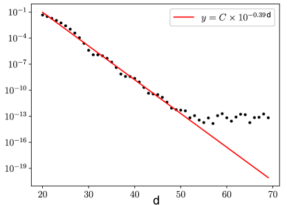
Theorem 3.1 is not optimal. One one hand, it overestimates the error for large times: both the numerical and exact solutions converge to stationary solutions as t𝑡t\to\infty, so we expect the error u(t)ud(t)2superscriptnorm𝑢𝑡subscript𝑢𝑑𝑡2\|u(t)-u_{d}(t)\|^{2} to tend to finite limit when t𝑡t\to\infty. Although the error between the stationary solutions can be bounded similarly to the transient error, see remark B.1, we have not obtained a result that combines both errors; we plan to return to this interesting question in future work. On the other hand, the bound on the transient error of theorem 3.1 is probably not sharp. Indeed, when the initial condition u0subscript𝑢0u_{0} is smooth and, together with all its derivatives, decreases exponentially as x𝑥x\to\infty, theorem 3.1 implies only that the error decreases faster than any negative power of d𝑑d. In most practical examples, however, we observed numerically that the convergence is in fact exponential.

Remark 3.3.

The condition that u0Hm(𝐑;m,x)subscript𝑢0superscript𝐻𝑚𝐑𝑚subscript𝑥u_{0}\in H^{m}(\mathbf{R};m,\mathcal{H}_{x}) is quite restrictive. It requires in particular that u0L2(𝐑)subscript𝑢0superscript𝐿2𝐑u_{0}\in L^{2}(\mathbf{R}), which is equivalent to requiring that ρ0L2(𝐑;ρs1)subscript𝜌0superscript𝐿2𝐑superscriptsubscript𝜌𝑠1\rho_{0}\in L^{2}(\mathbf{R};\rho_{s}^{-1}), because u0=ρ0/ρssubscript𝑢0subscript𝜌0subscript𝜌𝑠u_{0}=\rho_{0}/\sqrt{\rho_{s}} by definition. Though natural from an L2superscript𝐿2L^{2}-theory perspective, see [39, Sec. 4.5] and [35], this condition excludes a large class of initial conditions. If V(x)𝑉𝑥V(x) behaves as |x|4superscript𝑥4|x|^{4} as |x|𝑥|x|\to\infty, then it excludes Gaussian initial conditions, for example.

Remark 3.4.

An alternative manner of solving eq. 3.1 numerically is to approximate the eigenvalues and eigenfunctions of the operator xsubscript𝑥\mathcal{H}_{x} in terms of Hermite functions, after which integration in time becomes trivial. This approach requires finding (or approximating) the d+1𝑑1d+1 solutions (φdi,λdi)superscriptsubscript𝜑𝑑𝑖superscriptsubscript𝜆𝑑𝑖(\varphi_{d}^{i},\lambda_{d}^{i}), φdieVq/2𝐏(d)superscriptsubscript𝜑𝑑𝑖superscriptesubscript𝑉𝑞2𝐏𝑑\varphi_{d}^{i}\in\operatorname{e}^{-V_{q}/2}\,\mathbf{P}(d), 0id0𝑖𝑑0\leq i\leq d, of the eigenvalue problem

xφdi,wd=λdiφdi,wdwdeVq/2𝐏(d).formulae-sequencesubscript𝑥superscriptsubscript𝜑𝑑𝑖subscript𝑤𝑑superscriptsubscript𝜆𝑑𝑖superscriptsubscript𝜑𝑑𝑖subscript𝑤𝑑for-allsubscript𝑤𝑑superscriptesubscript𝑉𝑞2𝐏𝑑\left\langle{\mathcal{H}_{x}\,\varphi_{d}^{i},w_{d}}\right\rangle=\lambda_{d}^{i}\left\langle{\varphi_{d}^{i},w_{d}}\right\rangle\quad\forall w_{d}\in\operatorname{e}^{-V_{q}/2}\,\mathbf{P}(d). (3.5)

Once these have been calculated, an approximation of the solution to eq. 3.2 is obtained simply as

ud(t)=i=0dc0iφdieλdit,c0i=u0,φdid^.formulae-sequencesubscript𝑢𝑑𝑡superscriptsubscript𝑖0𝑑subscript𝑐0𝑖superscriptsubscript𝜑𝑑𝑖superscriptesubscriptsuperscript𝜆𝑖𝑑𝑡subscript𝑐0𝑖subscriptsubscript𝑢0superscriptsubscript𝜑𝑑𝑖^𝑑u_{d}(t)=\sum_{i=0}^{d}c_{0i}\,\varphi_{d}^{i}\,\operatorname{e}^{\lambda^{i}_{d}\,t},\quad c_{0i}=\left\langle{u_{0},\varphi_{d}^{i}}\right\rangle_{\hat{d}}. (3.6)

It is readily seen that udsubscript𝑢𝑑u_{d}, defined by this equation, is also the unique solution of (3.3a). This is the approach taken in [7] for the calculation of drift and diffusion coefficients in the diffusion approximation of kinetic equations. While equivalent, this methodology is more computationally expensive because it requires the full solution of the eigenvalue problem (3.5).

3.2 McKean–Vlasov equation with white noise

In the presence of an interaction term, the Fokker–Planck equation becomes nonlinear:

ρt=x(Vρ+θ(xm(t))ρ+β1ρx)=:(xm)ρ,m(t)=𝐑xρdx.\mathchoice{\frac{\partial{\rho}}{\partial t}}{\partial_{t}\rho}{}{}=\mathchoice{\frac{\partial{}}{\partial x}}{\partial_{x}}{}{}\left(V^{\prime}\,\rho+\theta(x-m(t))\,\rho+\beta^{-1}\mathchoice{\frac{\partial{\rho}}{\partial x}}{\partial_{x}\rho}{}{}\right)=:(\mathcal{L}_{x}^{m})^{*}\rho,\quad m(t)=\int_{\mathbf{R}}x\,\rho\,\mathrm{d}x. (3.7)

For this equation the weighted L2(𝐑;eV)superscript𝐿2𝐑superscripte𝑉L^{2}(\mathbf{R};\operatorname{e}^{V}) energy estimate of the linear case (B.7) does not hold, and there is therefore no longer a natural space for the Galerkin approximation. Because of this, and since we would like to employ the spectral numerical method with Gaussian initial conditions, which is not possible with a variational formulation of the type (3.3) in view of remark 3.3, we will use Hermite functions to approximate the solution to eq. 3.7 directly, i.e. we will look for an approximate solution in the space eVq/2𝐏(d)superscriptesubscript𝑉𝑞2𝐏𝑑\operatorname{e}^{-V_{q}/2}\,\mathbf{P}(d). The variational formulation corresponding to the Galerkin approximation is then to find ρeVq/2𝐏(d)𝜌superscriptesubscript𝑉𝑞2𝐏𝑑\rho\in\operatorname{e}^{-V_{q}/2}\,\mathbf{P}(d) such that

ρdt,wdsubscript𝜌𝑑𝑡subscript𝑤𝑑\displaystyle\left\langle{\mathchoice{\frac{\partial{\rho_{d}}}{\partial t}}{\partial_{t}\rho_{d}}{}{},w_{d}}\right\rangle =(xmd)ρd,wdabsentsuperscriptsuperscriptsubscript𝑥subscript𝑚𝑑subscript𝜌𝑑subscript𝑤𝑑\displaystyle=\left\langle{(\mathcal{L}_{x}^{m_{d}})^{*}\rho_{d},w_{d}}\right\rangle\qquad wdeVq/2𝐏(d),for-allsubscript𝑤𝑑superscriptesubscript𝑉𝑞2𝐏𝑑\displaystyle\forall w_{d}\in\operatorname{e}^{-V_{q}/2}\,\mathbf{P}(d), (3.8a)
mdsubscript𝑚𝑑\displaystyle\quad m_{d} =x,ρdd^missing1,ρdd^missing𝐑xρddx𝐑ρddx,absentsubscript𝑥subscript𝜌𝑑^𝑑missingsubscript1subscript𝜌𝑑^𝑑missingsubscript𝐑𝑥subscript𝜌𝑑differential-d𝑥subscript𝐑subscript𝜌𝑑differential-d𝑥\displaystyle=\frac{\left\langle{x,\rho_{d}}\right\rangle_{\hat{d}}missing}{\left\langle{1,\rho_{d}}\right\rangle_{\hat{d}}missing}\approx\frac{\int_{\mathbf{R}}x\,\rho_{d}\,\mathrm{d}x}{\int_{\mathbf{R}}\rho_{d}\,\mathrm{d}x}, (3.8b)
ρd(0),wdsubscript𝜌𝑑0subscript𝑤𝑑\displaystyle\left\langle{\rho_{d}(0),w_{d}}\right\rangle =ρ0,wdd^absentsubscriptsubscript𝜌0subscript𝑤𝑑^𝑑\displaystyle=\left\langle{\rho_{0},w_{d}}\right\rangle_{\hat{d}}\qquad wdeVq/2𝐏(d).for-allsubscript𝑤𝑑superscriptesubscript𝑉𝑞2𝐏𝑑\displaystyle\forall w_{d}\in\operatorname{e}^{-V_{q}/2}\,\mathbf{P}(d). (3.8c)

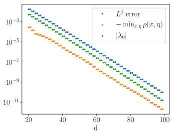
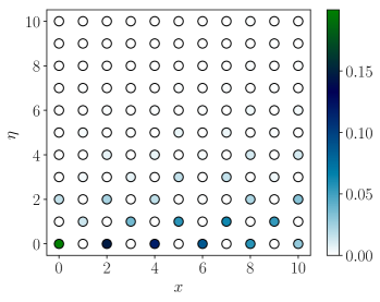
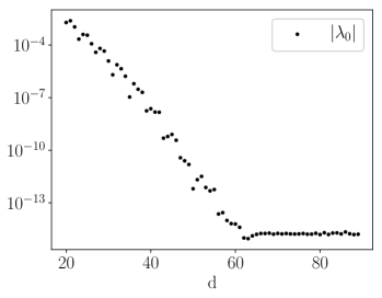
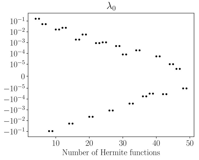
Dividing by 1,ρdd^subscript1subscript𝜌𝑑^𝑑\left\langle{1,\rho_{d}}\right\rangle_{\hat{d}} in eq. 3.8b is useful to account for changes in the total mass of ρdsubscript𝜌𝑑\rho_{d}, which can compromise the accuracy of the method when d𝑑d is low, but doing so becomes unnecessary for large enough d𝑑d. In contrast with the operator xsubscript𝑥\mathcal{H}_{x} in eq. 3.3a, the operator (xmd)superscriptsuperscriptsubscript𝑥subscript𝑚𝑑(\mathcal{L}_{x}^{m_{d}})^{*} is not selfadjoint in L2(𝐑)superscript𝐿2𝐑L^{2}(\mathbf{R}), and therefore the associated stiffness matrix is not symmetric. In addition, the quadratic form (xm),\left\langle{(\mathcal{L}_{x}^{m})^{*}\cdot,\cdot}\right\rangle is not necessarily negative for the usual L2(𝐑)superscript𝐿2𝐑L^{2}(\mathbf{R}) inner product, and indeed we observe numerically that the eigenvalue with smallest real part of the discrete operator is often negative, although small when d𝑑d is large enough. This is illustrated in fig. 3 for the same parameters as in the subsequent convergence study.
Refer to caption
(a) Eigenvalue with smallest real part of Π^d(xm)Π^dsubscript^Π𝑑superscriptsuperscriptsubscript𝑥𝑚subscript^Π𝑑-\hat{\Pi}_{d}\,(\mathcal{L}_{x}^{m})^{*}\,\hat{\Pi}_{d} for m=0𝑚0m=0. A mixed scale, linear in the interval [105,105]superscript105superscript105[-10^{-5},10^{-5}] and logarithmic elsewhere, is used for the y𝑦y axis.
Refer to caption
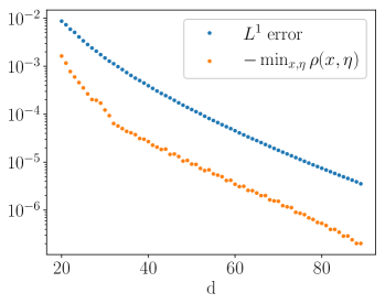
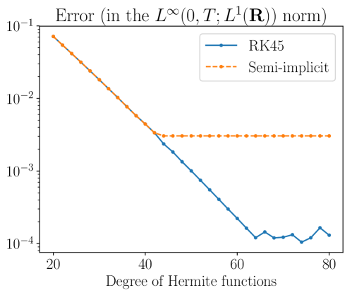
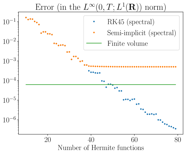
(b) Error of the Hermite Galerkin discretization, with either RK45 or the semi-implicit method (3.9), against degree of approximation (d𝑑d), and comparison with the error of the finite volume scheme from [8].
Figure 3: Study of the Galerkin approximation (3.8).

For the integration in time, we used either the RK45 method (using the solve_ivp method from the SciPy integrate module), or a linear semi-implicit method obtained by treating mdsubscript𝑚𝑑m_{d} explicitly and the other terms implicitly at each time step. The former is most useful when an accurate time-dependent solution is required, while the latter enables the use of larger time steps and is therefore more convenient when only the steady-state solution is sought, as will be the case for the construction of bifurcation diagrams. Denoting the time step by ΔtΔ𝑡\Delta t and the Galerkin approximation of ρd(nΔt)subscript𝜌𝑑𝑛Δ𝑡\rho_{d}(n\,\Delta t) by ρdnsuperscriptsubscript𝜌𝑑𝑛\rho_{d}^{n}, the semi-implicit method is based on obtaining ρdn+1superscriptsubscript𝜌𝑑𝑛1\rho_{d}^{n+1} by solving:

ρdn+1ρdn,wdsuperscriptsubscript𝜌𝑑𝑛1superscriptsubscript𝜌𝑑𝑛subscript𝑤𝑑\displaystyle\left\langle{\rho_{d}^{n+1}-\rho_{d}^{n},w_{d}}\right\rangle =Δt(xmdn)ρdn+1,wdwdeVq/2𝐏(d),formulae-sequenceabsentΔ𝑡superscriptsuperscriptsubscript𝑥superscriptsubscript𝑚𝑑𝑛superscriptsubscript𝜌𝑑𝑛1subscript𝑤𝑑for-allsubscript𝑤𝑑superscriptesubscript𝑉𝑞2𝐏𝑑\displaystyle=\Delta t\,\left\langle{(\mathcal{L}_{x}^{m_{d}^{n}})^{*}\rho_{d}^{n+1},w_{d}}\right\rangle\qquad\forall w_{d}\in\operatorname{e}^{-V_{q}/2}\,\mathbf{P}(d), (3.9a)
mdn+1superscriptsubscript𝑚𝑑𝑛1\displaystyle\quad m_{d}^{n+1} =x,ρdn+1d^missing1,ρdn+1d^missing.absentsubscript𝑥superscriptsubscript𝜌𝑑𝑛1^𝑑missingsubscript1superscriptsubscript𝜌𝑑𝑛1^𝑑missing\displaystyle=\frac{\left\langle{x,\rho_{d}^{n+1}}\right\rangle_{\hat{d}}missing}{\left\langle{1,\rho_{d}^{n+1}}\right\rangle_{\hat{d}}missing}. (3.9b)

Convergence study

The analysis of the Hermite spectral method for general types of McKean–Vlasov equations will not be presented here. For the purposes of this work, it will be sufficient to present a detailed numerical study of the convergence of the method. To study empirically the validity of the Galerkin method (3.8) and of the associated time-stepping scheme (3.9), we compare our method with the positivity preserving, entropy decreasing finite volume method proposed in [8] for nonlinear, nonlocal gradient PDEs111We reiterate the fact that one of the main advantages of our numerical method is that it does not require that the PDE has a gradient flow structure. . The parameters used here are β=3𝛽3\beta=3, θ=1𝜃1\theta=1, and the initial condition was the Gaussian 𝒩(101,1)𝒩superscript1011\mathcal{N}(10^{-1},1). The same time points were used for the finite volume method and semi-implicit Galerkin method (with a mean time step of approximately 0.002), and for RK45 the absolute and relative tolerances were both set to 1011superscript101110^{-11}. For the finite volume method, 600 equidistant mesh points were used between x=6𝑥6x=-6 and x=6𝑥6x=6.

Figure 3 presents the L(0,T;L1(𝐑))superscript𝐿0𝑇superscript𝐿1𝐑L^{\infty}(0,T;L^{1}(\mathbf{R})) norm of the errors associated with the solutions obtained, for values of d𝑑d, the degree of Hermite polynomials used, ranging from 101010 to 808080. A very accurate solution, obtained by using our spectral method with d=120𝑑120d=120, was employed for the calculation of the errors. We observe that, as d𝑑d increases initially, the solutions obtained using the semi-implicit (3.9) and the RK45 methods are indistinguishable and converge exponentially fast. From d40𝑑40d\approx 40, the accuracy of the semi-implicit method no longer improves, indicating that the error introduced by the time-stepping scheme dominates from that point on. From d50𝑑50d\approx 50, the Galerkin/RK45 approximation becomes more precise than the finite volume method. We therefore conclude that an accuracy as good as that obtained using the finite volume scheme can be reached with roughly ten times fewer unknowns using the spectral discretization (3.8). Our spectral method also enjoys a low computational cost: it ran in only about a minute with a Intel i7-3770 processor, even for a value of d𝑑d as high as 80, whereas the finite volume simulation took over an hour.

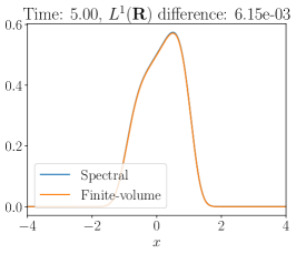
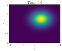
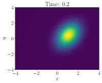
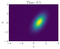
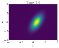
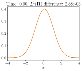
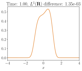
Figure 4 presents snapshots of the solutions at different times. We observe that, although the number of Hermite functions employed in the expansion is relatively low (=25), the solutions are in extremely good agreement.
Refer to caption
Refer to caption
Refer to caption
Figure 4: Snapshots of the solution to (3.7) using either the finite volume method from [8] or the Galerkin approximation (3.8) with the RK45 method and 25 Hermite functions.

In the simulations presented in this section, the scaling factor was set to σ2=110superscript𝜎2110\sigma^{2}=\frac{1}{10}. As discussed in appendix A, choosing this factor appropriately can significantly improve the accuracy of the method. In particular, given that the solution to eq. 3.7 decreases rapidly as |x|𝑥\left|x\right|\to\infty, σ𝜎\sigma should decrease with d𝑑d, with the optimal scaling being σdproportional-to𝜎𝑑\sigma\propto\sqrt{d}, as demonstrated in [46]. For convergence studies, however, it is convenient to use a fixed σ𝜎\sigma, first because this is assumed by most convergence results (such as theorem 3.1) and, second, because this simplifies the calculation of the matrices involved in the Galerkin formulation (only the last row and the last column have to be calculated upon incrementing d𝑑d).

Remark 3.5 (Computational considerations).

Discretizing the operators appearing in the Galerkin approximations (3.3a) and (3.8) requires the calculation of multiple matrices corresponding to operators of the type Πd(fx)ΠdsubscriptΠ𝑑𝑓subscript𝑥subscriptΠ𝑑\Pi_{d}\,\left(f\,\partial_{x}\right)\Pi_{d}, where f𝑓f is a polynomial and ΠdsubscriptΠ𝑑\Pi_{d} is the L2(𝐑;eVq)superscript𝐿2𝐑superscriptesubscript𝑉𝑞L^{2}(\mathbf{R};\operatorname{e}^{-V_{q}}) projection operator onto 𝐏(d)𝐏𝑑\mathbf{P}(d). These calculations can be carried out by noticing that

Πd(fdmdxm)Πd=(ΠdfΠd)(ΠddmdxmΠd).subscriptΠ𝑑𝑓superscriptd𝑚dsuperscript𝑥𝑚subscriptΠ𝑑subscriptΠ𝑑𝑓subscriptΠ𝑑subscriptΠ𝑑superscriptd𝑚dsuperscript𝑥𝑚subscriptΠ𝑑\Pi_{d}\,\left(f\,\mathchoice{\frac{\mathrm{d}^{m}{}}{\mathrm{d}x^{m}}}{\mathrm{d}_{x}^{m}}{}{}\right)\Pi_{d}=\left(\Pi_{d}\,f\,\Pi_{d}\right)\,\left(\Pi_{d}\mathchoice{\frac{\mathrm{d}^{m}{}}{\mathrm{d}x^{m}}}{\mathrm{d}_{x}^{m}}{}{}\Pi_{d}\right).

The matrix representation of the first operator on the right-hand side, in a basis of Hermite polynomials, can be obtained from the Hermite transform of f𝑓f. The matrix representation of the second operator, on the other hand, is a matrix with zero entries everywhere except on the m𝑚m-th superdiagonal, in view of the recursion relation (A.2).

3.3 Linear Fokker–Planck equation with colored noise

In this section, we turn our attention to the case of Gaussian or non-Gaussian colored noise given in terms of overdamped Langevin dynamics. The case of harmonic noise can be treated in a similar fashion, and for conciseness we do not present the associated Galerkin formulation explicitly here. We start by considering the linear (without the interaction term) Fokker–Planck equation with colored noise:

ρt=x(Vxρζε2β1ηρ)+1ε2η(Vηρ+ρη)=:ερ.\mathchoice{\frac{\partial{\rho}}{\partial t}}{\partial_{t}\rho}{}{}=\mathchoice{\frac{\partial{}}{\partial x}}{\partial_{x}}{}{}\left(\mathchoice{\frac{\partial{V}}{\partial x}}{\partial_{x}V}{}{}\,\rho-\frac{\zeta}{\varepsilon}\,\sqrt{2\,\beta^{-1}}\eta\,\rho\right)+\frac{1}{\varepsilon^{2}}\,\mathchoice{\frac{\partial{}}{\partial\eta}}{\partial_{\eta}}{}{}\,\left(V_{\eta}^{\prime}\,\rho+\mathchoice{\frac{\partial{\rho}}{\partial\eta}}{\partial_{\eta}\rho}{}{}\right)=:\mathcal{L}_{\varepsilon}^{*}\,\rho. (3.10)

We recall that ε2superscript𝜀2\varepsilon^{2} controls the correlation time of the colored noise and ζ𝜁\zeta is a parameter such that the white noise limit is recovered (with inverse temperature β𝛽\beta) when ε0𝜀0\varepsilon\to 0. We include ε𝜀\varepsilon in eq. 3.10 because, although we do not consider the white noise limit in this section, large values of ε𝜀\varepsilon are in general more difficult to tackle numerically, and it will be therefore convenient to use smaller correlation times in the numerical experiments below. The problem is now two-dimensional and the operator on the right-hand side of eq. 3.10 is no longer elliptic. In contrast with the white noise case, there does not exist an explicit formula for the steady-state solution for eq. 3.10.

The procedure for obtaining a Galerkin formulation is the same as in Subsection 3.1, except that we now use tensorized Hermite polynomials/functions. To retain some generality, we will consider that the Galerkin approximation space is of the form Sd=eU(x,η)/2eVq(x,η)/2𝐏(d)subscript𝑆𝑑superscripte𝑈𝑥𝜂2superscriptesubscript𝑉𝑞𝑥𝜂2𝐏subscript𝑑S_{d}=\operatorname{e}^{-U(x,\eta)/2}\,\operatorname{e}^{-V_{q}(x,\eta)/2}\,\mathbf{P}(\mathcal{I}_{d}) for some function U:𝐑2𝐑:𝑈maps-tosuperscript𝐑2𝐑U:\mathbf{R}^{2}\mapsto\mathbf{R}, a nondegenerate quadratic potential Vqsubscript𝑉𝑞V_{q} to be determined, and where 𝐏(d):=span{xαxηαη:(αx,αη)d}assign𝐏subscript𝑑span:superscript𝑥subscript𝛼𝑥superscript𝜂subscript𝛼𝜂subscript𝛼𝑥subscript𝛼𝜂subscript𝑑\mathbf{P}(\mathcal{I}_{d}):=\operatorname{span}\left\{x^{\alpha_{x}}\,\eta^{\alpha_{\eta}}:(\alpha_{x},\alpha_{\eta})\in\mathcal{I}_{d}\right\} for some index set d𝐍2subscript𝑑superscript𝐍2\mathcal{I}_{d}\subset\mathbf{N}^{2} that grows with d𝐍𝑑𝐍d\in\mathbf{N}. Compared to the one-dimensional case, there are now two scaling parameters, Vq:=x2/2σx2+η2/2ση2assignsubscript𝑉𝑞superscript𝑥22superscriptsubscript𝜎𝑥2superscript𝜂22superscriptsubscript𝜎𝜂2V_{q}:=x^{2}/2\sigma_{x}^{2}+\eta^{2}/2\sigma_{\eta}^{2}. The Galerkin approximation we propose consists in finding ρdSdsubscript𝜌𝑑subscript𝑆𝑑\rho_{d}\in S_{d} such that

ρdt,wdeU=subscriptsubscript𝜌𝑑𝑡subscript𝑤𝑑superscripte𝑈absent\displaystyle\left\langle{\mathchoice{\frac{\partial{\rho_{d}}}{\partial t}}{\partial_{t}\rho_{d}}{}{},w_{d}}\right\rangle_{\operatorname{e}^{U}}= ερd,wdeUwdSd,t>0,formulae-sequencesubscriptsuperscriptsubscript𝜀subscript𝜌𝑑subscript𝑤𝑑superscripte𝑈for-allsubscript𝑤𝑑subscript𝑆𝑑for-all𝑡0\displaystyle\left\langle{\mathcal{L}_{\varepsilon}^{*}\,\rho_{d},w_{d}}\right\rangle_{\operatorname{e}^{U}}\qquad\forall w_{d}\in S_{d},\quad\forall t>0, (3.11)

with appropriate initial conditions. The choice of the weight eUsuperscripte𝑈\operatorname{e}^{U} in the inner products of eq. 3.11 is motivated by the fact that differential operators admit sparse representations in the Hermite-type basis naturally associated with Sdsubscript𝑆𝑑S_{d}, and we note that eU(x,η)/2eVq(x,η)/2𝐏(𝐍2)superscripte𝑈𝑥𝜂2superscriptesubscript𝑉𝑞𝑥𝜂2𝐏superscript𝐍2\operatorname{e}^{-U(x,\eta)/2}\,\operatorname{e}^{-V_{q}(x,\eta)/2}\,\mathbf{P}(\mathbf{N}^{2}), where 𝐏(𝐍2)𝐏superscript𝐍2\mathbf{P}(\mathbf{N}^{2}) is the space of polynomials in two dimensions, is dense in L2(𝐑2;eU)superscript𝐿2superscript𝐑2superscripte𝑈L^{2}(\mathbf{R}^{2};\operatorname{e}^{U}). In practice, we obtain ρdsubscript𝜌𝑑\rho_{d} as eU(x,η)/2eVq(x,η)/2vdsuperscripte𝑈𝑥𝜂2superscriptesubscript𝑉𝑞𝑥𝜂2subscript𝑣𝑑\operatorname{e}^{-U(x,\eta)/2}\,\operatorname{e}^{-V_{q}(x,\eta)/2}\,v_{d}, where vdsubscript𝑣𝑑v_{d} is obtained by solving

vdt,wdeVq=subscriptsubscript𝑣𝑑𝑡subscript𝑤𝑑superscriptesubscript𝑉𝑞absent\displaystyle\left\langle{\mathchoice{\frac{\partial{v_{d}}}{\partial t}}{\partial_{t}v_{d}}{}{},w_{d}}\right\rangle_{\operatorname{e}^{-V_{q}}}= εvd,wdeVqwd𝐏(d),t>0,formulae-sequencesubscriptsubscript𝜀subscript𝑣𝑑subscript𝑤𝑑superscriptesubscript𝑉𝑞for-allsubscript𝑤𝑑𝐏subscript𝑑for-all𝑡0\displaystyle\left\langle{\mathcal{H}_{\varepsilon}\,v_{d},w_{d}}\right\rangle_{\operatorname{e}^{-V_{q}}}\qquad\forall w_{d}\in\mathbf{P}(\mathcal{I}_{d}),\quad\forall t>0, (3.12)

where, for a test function φ𝜑\varphi, εφ:=(eU/2eVq/2)ε(eU/2eVq/2φ)assignsubscript𝜀𝜑superscripte𝑈2superscriptesubscript𝑉𝑞2superscriptsubscript𝜀superscripte𝑈2superscriptesubscript𝑉𝑞2𝜑\mathcal{H}_{\varepsilon}\varphi:=(\operatorname{e}^{U/2}\,\operatorname{e}^{V_{q}/2})\mathcal{L}_{\varepsilon}^{*}\,(\operatorname{e}^{-U/2}\,\operatorname{e}^{-V_{q}/2}\,\varphi), and the basis functions used for eq. 3.12 are Hermite polynomials orthonormal with respect to the Gaussian weight eVqsuperscriptesubscript𝑉𝑞\operatorname{e}^{-V_{q}}. Regarding the index set, several choices are possible, with the simplest ones being the triangle {α𝐍2:|α|1d}conditional-set𝛼superscript𝐍2subscript𝛼1𝑑\{\alpha\in\mathbf{N}^{2}:\left|\alpha\right|_{1}\leq d\} and the square {α𝐍2:|α|d}conditional-set𝛼superscript𝐍2subscript𝛼𝑑\{\alpha\in\mathbf{N}^{2}:\left|\alpha\right|_{\infty}\leq d\}, see figs. 15 and 16 below. We demonstrate in Section 4 that, in order to study the limit ε0𝜀0\varepsilon\to 0, a rectangle-shaped index set is usually the only suitable choice. When studying the behavior as d𝑑d increases, however, we observed spectral convergence irrespectively of the index set utilized.

Clearly, it is necessary that ρL2(𝐑2;eU)𝜌superscript𝐿2superscript𝐑2superscripte𝑈\rho\in L^{2}(\mathbf{R}^{2};\operatorname{e}^{U}) for the Galerkin discretization (3.11) to produce good results. Since the 1/ε21superscript𝜀21/\varepsilon^{2} part of the operator on the right-hand side of eq. 3.10, 0=η(Vη(η)+η)\mathcal{L}_{0}^{*}\cdot=\mathchoice{\frac{\partial{}}{\partial\eta}}{\partial_{\eta}}{}{}(V_{\eta}^{\prime}(\eta)\cdot+\,\mathchoice{\frac{\partial{}}{\partial\eta}}{\partial_{\eta}}{}{}\cdot), is selfadjoint in L2(𝐑;eUx(x)/2Vη(η)/2)superscript𝐿2𝐑superscriptesubscript𝑈𝑥𝑥2subscript𝑉𝜂𝜂2L^{2}(\mathbf{R};\operatorname{e}^{-U_{x}(x)/2-V_{\eta}(\eta)/2}) for any choice of Uxsubscript𝑈𝑥U_{x}, it is natural to choose eU(x,η)/2=eUx(x)/2Vη(η)/2superscripte𝑈𝑥𝜂2superscriptesubscript𝑈𝑥𝑥2subscript𝑉𝜂𝜂2\operatorname{e}^{-U(x,\eta)/2}=\operatorname{e}^{-U_{x}(x)/2-V_{\eta}(\eta)/2} for some one-dimensional potential Uxsubscript𝑈𝑥U_{x}. This guarantees that the matrix representation of 0superscriptsubscript0\mathcal{L}_{0}^{*} is symmetric and negative semi-definite, but this is not a requirement.

The performance of the Galerkin approximation (3.11) is investigated through numerical experiments in appendix C. An asymptotic analysis of the numerical method in the limit as ε0𝜀0\varepsilon\to 0 is presented in [22], which is a longer version of this paper.

3.4 McKean–Vlasov equation with colored noise

We consider now the nonlinear McKean–Vlasov initial value problem with OU noise: recalling that ζ=1/2𝜁12\zeta=1/\sqrt{2} in this case,

ρt=x(Vxρ+θ(xm(t))ρ1εβ1ηρ)+1ε2η(ηρ+ρη),𝜌𝑡𝑥𝑉𝑥𝜌𝜃𝑥𝑚𝑡𝜌1𝜀superscript𝛽1𝜂𝜌1superscript𝜀2𝜂𝜂𝜌𝜌𝜂\displaystyle\mathchoice{\frac{\partial{\rho}}{\partial t}}{\partial_{t}\rho}{}{}=\mathchoice{\frac{\partial{}}{\partial x}}{\partial_{x}}{}{}\left(\mathchoice{\frac{\partial{V}}{\partial x}}{\partial_{x}V}{}{}\,\rho+\theta\,(x-m(t))\,\rho-\frac{1}{\varepsilon}\,\sqrt{\beta^{-1}}\,\eta\,\rho\right)+\frac{1}{\varepsilon^{2}}\,\mathchoice{\frac{\partial{}}{\partial\eta}}{\partial_{\eta}}{}{}\,\left(\eta\,\rho+\mathchoice{\frac{\partial{\rho}}{\partial\eta}}{\partial_{\eta}\rho}{}{}\right), (3.13a)
m(t)=𝐑𝐑xρ(x,η,t)dηdx,𝑚𝑡subscript𝐑subscript𝐑𝑥𝜌𝑥𝜂𝑡differential-d𝜂differential-d𝑥\displaystyle m(t)=\int_{\mathbf{R}}\int_{\mathbf{R}}x\,\rho(x,\eta,t)\,\mathrm{d}\eta\,\mathrm{d}x, (3.13b)
ρ(x,η,t=0)=ρ0(x,η),𝜌𝑥𝜂𝑡0subscript𝜌0𝑥𝜂\displaystyle\rho(x,\eta,t=0)=\rho_{0}(x,\eta), (3.13c)

for some initial distribution ρ0(x,η)subscript𝜌0𝑥𝜂\rho_{0}(x,\eta) such that the noise is not necessarily started at stationarity. The method that we use in this case, which applies mutatis mutandis to the other noise models, is the same as in eq. 3.11, with the addition of the interaction term, and we use the same time-stepping schemes as in Subsection 3.1.

Numerical experiments, testing the convergence of the method for the two time-stepping schemes, are presented in appendix C.

3.5 Monte Carlo simulations

We will compare the bifurcation diagrams obtained using the spectral method described above to those obtained by direct MC simulations of the system of interacting particles (2.1). We use the Euler–Maruyama method:

Xk+1i=XkiV(Xki)Δtθ(Xki1Nj=1NXkj)Δt+ζε2β1ηkiΔt,superscriptsubscript𝑋𝑘1𝑖superscriptsubscript𝑋𝑘𝑖superscript𝑉superscriptsubscript𝑋𝑘𝑖Δ𝑡𝜃superscriptsubscript𝑋𝑘𝑖1𝑁superscriptsubscript𝑗1𝑁superscriptsubscript𝑋𝑘𝑗Δ𝑡𝜁𝜀2superscript𝛽1superscriptsubscript𝜂𝑘𝑖Δ𝑡X_{k+1}^{i}=X_{k}^{i}-V^{\prime}(X_{k}^{i})\,\Delta t-\theta\left(X_{k}^{i}-\frac{1}{N}\sum_{j=1}^{N}X_{k}^{j}\right)\,\Delta t+\frac{\zeta}{\varepsilon}\,\sqrt{2\beta^{-1}}\,\eta_{k}^{i}\,\Delta t,

where ηkisuperscriptsubscript𝜂𝑘𝑖\eta_{k}^{i} is the appropriate projection of the stochastic process 𝐘tsubscript𝐘𝑡\boldsymbol{\mathbf{Y}}_{t}. In the case of Gaussian noise, this is discretized as follows

𝐘k+1i=𝐘ki+1ε2A𝐘kiΔt+1ε2ΔtDξ,superscriptsubscript𝐘𝑘1𝑖superscriptsubscript𝐘𝑘𝑖1superscript𝜀2𝐴superscriptsubscript𝐘𝑘𝑖Δ𝑡1𝜀2Δ𝑡𝐷𝜉\boldsymbol{\mathbf{Y}}_{k+1}^{i}=\boldsymbol{\mathbf{Y}}_{k}^{i}+\frac{1}{\varepsilon^{2}}A\,\boldsymbol{\mathbf{Y}}_{k}^{i}\,\Delta t+\frac{1}{\varepsilon}\,\sqrt{2\ \Delta t}\,D\xi,

where ξN(0,1)similar-to𝜉𝑁01\xi\sim N(0,1), and Xksubscript𝑋𝑘X_{k}, 𝐘ksubscript𝐘𝑘\boldsymbol{\mathbf{Y}}_{k} and ηksubscript𝜂𝑘\eta_{k} are the approximations to X(kΔt),𝐘(kΔt)𝑋𝑘Δ𝑡𝐘𝑘Δ𝑡X(k\Delta t),\,\boldsymbol{\mathbf{Y}}(k\Delta t) and η(kΔt)𝜂𝑘Δ𝑡\eta(k\Delta t), respectively. The time step used was always 𝒪(ε2)𝒪superscript𝜀2\mathcal{O}(\varepsilon^{2}), to ensure the accurate solution of the equation. This scheme has weak order of convergence one, see [24, 25], and we find that we capture the correct behavior as long as the time step is sufficiently small.

4 Asymptotic analysis for the Galerkin formulation

In Section 5, we will construct bifurcation diagrams of m𝑚m as a function of β𝛽\beta for different values of ε𝜀\varepsilon, and we will verify that the bifurcation diagram of the white noise case is recovered when ε0𝜀0\varepsilon\to 0. Since the spectral method presented in Section 3 will be used to that purpose, it is useful to study the behavior of the solution to the Galerkin formulation (3.11) in the limit ε0𝜀0\varepsilon\to 0, which is the purpose of this section. We will then confirm numerically the rates of convergence to the white noise limit presented in Subsection 2.2, i.e. 𝒪(ε2)𝒪superscript𝜀2\mathcal{O}(\varepsilon^{2}) for Ornstein–Uhlenbeck noise and 𝒪(ε4)𝒪superscript𝜀4\mathcal{O}(\varepsilon^{4}) for harmonic noise.

For simplicity, we confine ourselves for the analysis to the case where the noise process is one-dimensional and the weight function eU(x,η)/2superscripte𝑈𝑥𝜂2\operatorname{e}^{-U(x,\eta)/2} can be decomposed as eU(x,η)/2=eUx(x)/2eVη(η)/2superscripte𝑈𝑥𝜂2superscriptesubscript𝑈𝑥𝑥2superscriptesubscript𝑉𝜂𝜂2\operatorname{e}^{-U(x,\eta)/2}=\operatorname{e}^{-U_{x}(x)/2}\,\operatorname{e}^{-V_{\eta}(\eta)/2}. As before, Π^dsubscript^Π𝑑\hat{\Pi}_{d} denotes the L2(𝐑2;eU)superscript𝐿2superscript𝐑2superscripte𝑈L^{2}(\mathbf{R}^{2};\operatorname{e}^{U}) projection operator on the space of Hermite functions (with appropriate scalings). Decomposing the operator (Π^dεΠ^d)subscript^Π𝑑superscriptsubscript𝜀subscript^Π𝑑(\hat{\Pi}_{d}\,\mathcal{L}_{\varepsilon}^{*}\,\hat{\Pi}_{d}) in eq. 3.11 in powers of ε𝜀\varepsilon, we obtain the equation

ρdt=(Π^dεΠ^d)ρdsubscript𝜌𝑑𝑡subscript^Π𝑑superscriptsubscript𝜀subscript^Π𝑑subscript𝜌𝑑\displaystyle\mathchoice{\frac{\partial{\rho_{d}}}{\partial t}}{\partial_{t}\rho_{d}}{}{}=(\hat{\Pi}_{d}\,\mathcal{L}_{\varepsilon}^{*}\,\hat{\Pi}_{d})\,\rho_{d} =Π^d(1ε20+1ε1+2)Π^dρd,absentsubscript^Π𝑑1superscript𝜀2superscriptsubscript01𝜀superscriptsubscript1superscriptsubscript2subscript^Π𝑑subscript𝜌𝑑\displaystyle=\hat{\Pi}_{d}\,\left(\frac{1}{\varepsilon^{2}}\mathcal{L}_{0}^{*}+\frac{1}{\varepsilon}\mathcal{L}_{1}^{*}+\mathcal{L}_{2}^{*}\right)\hat{\Pi}_{d}\,\rho_{d},
=:(1ε2^0+1ε^1+^2)ρd.\displaystyle=:\left(\frac{1}{\varepsilon^{2}}\hat{\mathcal{L}}_{0}+\frac{1}{\varepsilon}\hat{\mathcal{L}}_{1}+\hat{\mathcal{L}}_{2}\right)\rho_{d}.

As a consequence of the choice of eUsuperscripte𝑈\operatorname{e}^{U}, the largest (sign included) eigenvalue of ^0subscript^0\hat{\mathcal{L}}_{0} is a nonpositive, nondecreasing function of d𝑑d. Since we cannot expect the leading order term of the discrete generator to have an eigenvalue exactly equal to 0, we look for a solution of the form ρd=e|λ0,d|t/ε2(ϱ0+εϱ1+ε2ϱ2+)subscript𝜌𝑑superscriptesubscript𝜆0𝑑𝑡superscript𝜀2subscriptitalic-ϱ0𝜀subscriptitalic-ϱ1superscript𝜀2subscriptitalic-ϱ2\rho_{d}=\operatorname{e}^{-\left|\lambda_{0,d}\right|\,t/\varepsilon^{2}}(\varrho_{0}+\varepsilon\,\varrho_{1}+\varepsilon^{2}\,\varrho_{2}+\dotsb), where λ0,dsubscript𝜆0𝑑\lambda_{0,d} is the largest eigenvalue of ^0subscript^0\hat{\mathcal{L}}_{0}. Denoting by idid\operatorname{id} the identity operator and gathering equal powers of ε𝜀\varepsilon, we obtain the equations:

0=(0^+|λ0,d|id)ϱ0,0^subscript0subscript𝜆0𝑑idsubscriptitalic-ϱ0\displaystyle 0=\left(\hat{\mathcal{L}_{0}}+\left|\lambda_{0,d}\right|\,\operatorname{id}\right)\,\varrho_{0}, (4.2a)
0=(0^+|λ0,d|id)ϱ1+1^ϱ0,0^subscript0subscript𝜆0𝑑idsubscriptitalic-ϱ1^subscript1subscriptitalic-ϱ0\displaystyle 0=\left(\hat{\mathcal{L}_{0}}+\left|\lambda_{0,d}\right|\,\operatorname{id}\right)\,\varrho_{1}+\hat{\mathcal{L}_{1}}\,\varrho_{0}, (4.2b)
ϱit=(0^+|λ0,d|id)ϱi+2+1^ϱi+1+2^ϱi,i=0,1,formulae-sequencesubscriptitalic-ϱ𝑖𝑡^subscript0subscript𝜆0𝑑idsubscriptitalic-ϱ𝑖2^subscript1subscriptitalic-ϱ𝑖1^subscript2subscriptitalic-ϱ𝑖𝑖01\displaystyle\mathchoice{\frac{\partial{\varrho_{i}}}{\partial t}}{\partial_{t}\varrho_{i}}{}{}=\left(\hat{\mathcal{L}_{0}}+\left|\lambda_{0,d}\right|\,\operatorname{id}\right)\,\varrho_{i+2}+\hat{\mathcal{L}_{1}}\,\varrho_{i+1}+\hat{\mathcal{L}_{2}}\,\varrho_{i},\qquad i=0,1,\dotsc (4.2c)

4.1 Suitable index sets

Let Hixsubscriptsuperscript𝐻𝑥𝑖H^{x}_{i} and Hjηsubscriptsuperscript𝐻𝜂𝑗H^{\eta}_{j} denote the (possibly rescaled) Hermite functions in the x𝑥x and η𝜂\eta directions, respectively. Let also i,ηsubscript𝑖𝜂\mathcal{I}_{i,\eta} be a slice of the index set, i,η:={j:(i,j)d}assignsubscript𝑖𝜂conditional-set𝑗𝑖𝑗subscript𝑑\mathcal{I}_{i,\eta}:=\{j:(i,j)\in\mathcal{I}_{d}\}, and ΠxdsubscriptΠ𝑥subscript𝑑\Pi_{x}\mathcal{I}_{d} be the projected index set given by {i:(j𝐍)[(i,j)d]}conditional-set𝑖𝑗𝐍delimited-[]𝑖𝑗subscript𝑑\{i:(\exists j\in\mathbf{N})[(i,j)\in\mathcal{I}_{d}]\}. Expanding ϱ0subscriptitalic-ϱ0\varrho_{0} in terms of the basis functions used for the Galerkin discretization in the first equation, we obtain

00\displaystyle 0 =(^0+|λ0,d|id)(i,j)dcij(eUx/2HixeVη/2Hjη)absentsubscript^0subscript𝜆0𝑑idsubscript𝑖𝑗subscript𝑑subscript𝑐𝑖𝑗superscriptesubscript𝑈𝑥2tensor-productsubscriptsuperscript𝐻𝑥𝑖superscript𝑒subscript𝑉𝜂2subscriptsuperscript𝐻𝜂𝑗\displaystyle=(\hat{\mathcal{L}}_{0}+\left|\lambda_{0,d}\right|\operatorname{id})\,\sum_{(i,j)\in\mathcal{I}_{d}}c_{ij}\,\left(\operatorname{e}^{-U_{x}/2}\,H^{x}_{i}\otimes e^{-V_{\eta}/2}\,H^{\eta}_{j}\right)
=iΠxdeUx/2Hix(ji,ηcijki,η(Ljk+|λ0,d|δjk)eVη/2Hkη),absentsubscript𝑖subscriptΠ𝑥subscript𝑑tensor-productsuperscriptesubscript𝑈𝑥2subscriptsuperscript𝐻𝑥𝑖subscript𝑗subscript𝑖𝜂subscript𝑐𝑖𝑗subscript𝑘subscript𝑖𝜂subscript𝐿𝑗𝑘subscript𝜆0𝑑subscript𝛿𝑗𝑘superscriptesubscript𝑉𝜂2subscriptsuperscript𝐻𝜂𝑘\displaystyle=\sum_{i\in\Pi_{x}\mathcal{I}_{d}}\operatorname{e}^{-U_{x}/2}\,H^{x}_{i}\otimes\left(\sum_{j\in\mathcal{I}_{i,\eta}}c_{ij}\sum_{k\in\mathcal{I}_{i,\eta}}(L_{jk}+\left|\lambda_{0,d}\right|\,\delta_{jk})\,\operatorname{e}^{-V_{\eta}/2}\,H^{\eta}_{k}\right),

where Ljk:=0(eVη/2Hjη),eVη/2HkηeVηassignsubscript𝐿𝑗𝑘subscriptsuperscriptsubscript0superscriptesubscript𝑉𝜂2subscriptsuperscript𝐻𝜂𝑗superscriptesubscript𝑉𝜂2subscriptsuperscript𝐻𝜂𝑘superscriptesubscript𝑉𝜂L_{jk}:=\left\langle{\mathcal{L}_{0}^{*}(\operatorname{e}^{-V_{\eta}/2}\,H^{\eta}_{j}),\operatorname{e}^{-V_{\eta}/2}\,H^{\eta}_{k}}\right\rangle_{\operatorname{e}^{V_{\eta}}}. Since {eUx/2Hix}iΠxdsubscriptsuperscriptesubscript𝑈𝑥2subscriptsuperscript𝐻𝑥𝑖𝑖subscriptΠ𝑥subscript𝑑\{\operatorname{e}^{-U_{x}/2}\,H^{x}_{i}\}_{i\in\Pi_{x}\mathcal{I}_{d}} are linearly independent, this implies that

ji,ηcij(Ljk+|λ0,d|δjk)=0,iΠxd,formulae-sequencesubscript𝑗subscript𝑖𝜂subscript𝑐𝑖𝑗subscript𝐿𝑗𝑘subscript𝜆0𝑑subscript𝛿𝑗𝑘0for-all𝑖subscriptΠ𝑥subscript𝑑\sum_{j\in\mathcal{I}_{i,\eta}}c_{ij}\,(L_{jk}+\left|\lambda_{0,d}\right|\,\delta_{jk})=0,\qquad\forall i\in\Pi_{x}\mathcal{I}_{d}, (4.3)

implying that, for all iΠxdfor-all𝑖subscriptΠ𝑥subscript𝑑\forall i\in\Pi_{x}\mathcal{I}_{d}, the vector of coefficients (cij)ji,ηsubscriptsubscript𝑐𝑖𝑗𝑗subscript𝑖𝜂{(c_{ij})}_{j\in\mathcal{I}_{i,\eta}} is in the kernel of the matrix (Ljk+|λ0,d|)j,ki,ηsubscriptsubscript𝐿𝑗𝑘subscript𝜆0𝑑𝑗𝑘subscript𝑖𝜂{(L_{jk}+\left|\lambda_{0,d}\right|)}_{j,k\in\mathcal{I}_{i,\eta}}. Therefore, if for some i𝑖i this matrix has full rank, then the corresponding Hermite coefficients must be 00. This is of particular relevance when the eigenfunction in the kernel of 0superscriptsubscript0\mathcal{L}_{0}^{*} cannot be exactly represented in terms of a finite number of the approximating basis functions, as is the case with the noise processes B and NS considered in Section 2.

Consider for example the case of a triangular index set. In this case the matrix Mi:=(Ljk+|λ0,d|)j,ki,ηassignsubscript𝑀𝑖subscriptsubscript𝐿𝑗𝑘subscript𝜆0𝑑𝑗𝑘subscript𝑖𝜂M_{i}:={(L_{jk}+\left|\lambda_{0,d}\right|)}_{j,k\in\mathcal{I}_{i,\eta}} is of shape d+1i×d+1i𝑑1𝑖𝑑1𝑖d+1-i\times d+1-i: incrementing i𝑖i by one corresponds to removing the last line last and last column of the matrix. Consequently, the maximal eigenvalue of Misubscript𝑀𝑖M_{i} (sign included), which we denote by λmax(i)subscript𝜆𝑖\lambda_{\max}(i), is a nonincreasing function of i𝑖i such that λmax(0)=0subscript𝜆00\lambda_{\max}(0)=0. In the case of noise model B, it holds that λmax(i)<0subscript𝜆𝑖0\lambda_{\max}(i)<0 for i>0𝑖0i>0 or i>1𝑖1i>1, depending on whether d𝑑d is even or odd. Consequently, in this case eq. 4.3 implies that cij=0subscript𝑐𝑖𝑗0c_{ij}=0 for these values of i𝑖i and all ji,η𝑗subscript𝑖𝜂j\in\mathcal{I}_{i,\eta}.

From this we conclude that, in order to capture the correct solution as ε0𝜀0\varepsilon\to 0, it is necessary to choose a rectangularly shaped index set, which is consistent with the fact that, in the limit ε0𝜀0\varepsilon\to 0, the solution can be expressed as a tensor product ρ(x,η)=ρx(x)ρη(η)subscript𝜌𝑥𝜂superscript𝜌𝑥𝑥superscript𝜌𝜂𝜂\rho_{\infty}(x,\eta)=\rho^{x}(x)\,\rho^{\eta}(\eta).

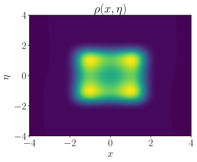
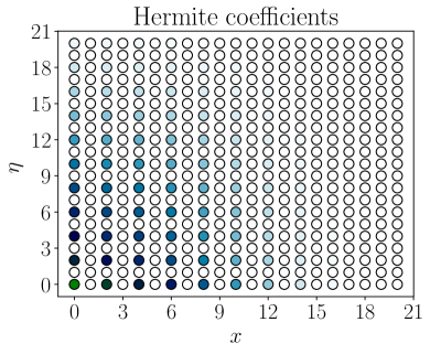
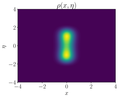
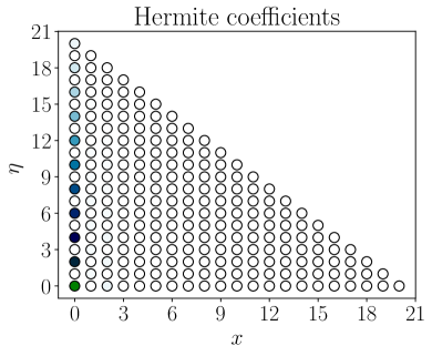
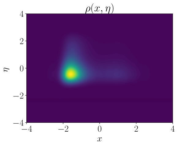
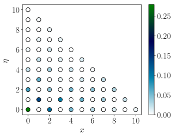
To illustrate the point made in the previous paragraph, we present side by side in fig. 5 the results of numerical experiments performed using either a triangular index set or a square index set, for the parameters ε=0.01𝜀0.01\varepsilon=0.01, d=20𝑑20d=20, β=15𝛽15\beta=15, θ=0𝜃0\theta=0, σx2=ση2=1/15superscriptsubscript𝜎𝑥2superscriptsubscript𝜎𝜂2115\sigma_{x}^{2}=\sigma_{\eta}^{2}=1/15, eUx(x)=1superscriptesubscript𝑈𝑥𝑥1\operatorname{e}^{-U_{x}(x)}=1. While the probability density obtained using a square index set is close to the exact solution and clearly exhibits four local maxima, the solution obtained using a triangle index set is concentrated around x=0𝑥0x=0, and all the associated Hermite coefficients cijsubscript𝑐𝑖𝑗c_{ij} with i>0𝑖0i>0 are very close to zero.

Refer to caption
Refer to caption
(a) Square index set.
Refer to caption
Refer to caption
(b) Triangle index set.
Figure 5: Comparison of the numerical solutions for the steady-state Fokker–Planck equation with the bistable noise model (model B in Section 2), using either a square index set or a triangle index set. While not obvious from the figures, in the former case it follows from the fact that ε=0.011𝜀0.01much-less-than1\varepsilon=0.01\ll 1 that the columns of Hermite coefficients in the η𝜂\eta direction are essentially colinear.

4.2 Effective drift and diffusion coefficients

We assume from now on that the index-set has a rectangular shape, d={0,1,,dx}×{0,1,,dη}subscript𝑑01subscript𝑑𝑥01subscript𝑑𝜂\mathcal{I}_{d}=\{0,1,\dotsc,d_{x}\}\times\{0,1,\dotsc,d_{\eta}\}. At the continuous, infinite dimensional level, the absence of an effective drift term for the models of the noise B and NS as ε0𝜀0\varepsilon\to 0 is ensured by the centering condition (2.3). Any deviation from zero would lead to an effective drift term, scaling as 1/ε1𝜀1/\varepsilon and proportional to

2β1ζ𝐑ηexp(βVη(η))dη.2superscript𝛽1𝜁subscript𝐑𝜂𝛽subscript𝑉𝜂𝜂differential-d𝜂\sqrt{2\,\beta^{-1}}\,\zeta\,\int_{\mathbf{R}}\eta\,\exp\left(-\beta V_{\eta}(\eta)\right)\,\mathrm{d}\eta.

At the finite-dimensional, numerical level, a parasitic effective drift can arise even when Vηsubscript𝑉𝜂V_{\eta} satisfies (2.3), as we demonstrate below. This can occur when Vηsubscript𝑉𝜂V_{\eta} is not an even function, and it is especially critical when the number of basis functions used to approximate the solution in the η𝜂\eta direction is relatively low, leading to a nonzero first moment of the approximate equilibrium probability density of the noise process. In these cases, it is useful to introduce an artificial drift term μd/εsubscript𝜇𝑑𝜀\mu_{d}/\varepsilon in Galerkin formulation, for some constant μdsubscript𝜇𝑑\mu_{d} to be determined. To formulate result 4.1 below, let φ0,dsubscript𝜑0𝑑\varphi_{0,d} denote the (assumed unique up to a sign) normalized one-dimensional eigenfunction associated with λ0,dsubscript𝜆0𝑑\lambda_{0,d},

φ0,d=argmaxφdSdηη,φdeVη=1eVη/2φd,eη2/4ση2>00φd,φdeVη,where Sdηη=eVη/2eη2/4ση2𝐏(dη).formulae-sequencesubscript𝜑0𝑑superscriptesubscript𝑉𝜂2subscript𝜑𝑑superscriptesuperscript𝜂24superscriptsubscript𝜎𝜂20subscriptargmaxsubscript𝜑𝑑superscriptsubscript𝑆subscript𝑑𝜂𝜂subscriptnormsubscript𝜑𝑑superscriptesubscript𝑉𝜂1subscriptsuperscriptsubscript0subscript𝜑𝑑subscript𝜑𝑑superscriptesubscript𝑉𝜂where superscriptsubscript𝑆subscript𝑑𝜂𝜂superscriptesubscript𝑉𝜂2superscriptesuperscript𝜂24superscriptsubscript𝜎𝜂2𝐏subscript𝑑𝜂\varphi_{0,d}=\underset{\left\langle{\operatorname{e}^{V_{\eta}/2}\,\varphi_{d},\operatorname{e}^{-\eta^{2}/4\sigma_{\eta}^{2}}}\right\rangle>0}{\operatorname*{arg\,max}_{\varphi_{d}\in S_{d_{\eta}}^{\eta},\,\|\varphi_{d}\|_{\operatorname{e}^{V_{\eta}}=1}}}\left\langle{\mathcal{L}_{0}^{*}\varphi_{d},\varphi_{d}}\right\rangle_{\operatorname{e}^{V_{\eta}}},\qquad\text{where }S_{d_{\eta}}^{\eta}=\operatorname{e}^{-V_{\eta}/2}\,\operatorname{e}^{-\eta^{2}/4\sigma_{\eta}^{2}}\,\mathbf{P}(d_{\eta}).
Result 4.1.

Let μdsubscript𝜇𝑑\mu_{d} be defined by

μd=2β1ζ𝐑ηφ0,d2eV(η)dη.subscript𝜇𝑑2superscript𝛽1𝜁subscript𝐑𝜂superscriptsubscript𝜑0𝑑2superscripte𝑉𝜂d𝜂\mu_{d}=-\sqrt{2\,\beta^{-1}}\,\zeta\,\int_{\mathbf{R}}\eta\,\varphi_{0,d}^{2}\,\operatorname{e}^{V(\eta)}\,\mathrm{d}\eta. (4.4)

Then, when ε1much-less-than𝜀1\varepsilon\ll 1, the solution ρdsubscript𝜌𝑑\rho_{d} of

ρdt=Π^d(ε+|λ0,d|id(μdε)x)Π^dρd,ρd(x,η,t=0)=ρd,0(x)φ0,d(η)formulae-sequencesubscript𝜌𝑑𝑡subscript^Π𝑑superscriptsubscript𝜀subscript𝜆0𝑑idsubscript𝜇𝑑𝜀𝑥subscript^Π𝑑subscript𝜌𝑑subscript𝜌𝑑𝑥𝜂𝑡0subscript𝜌𝑑0𝑥subscript𝜑0𝑑𝜂\displaystyle\mathchoice{\frac{\partial{\rho_{d}}}{\partial t}}{\partial_{t}\rho_{d}}{}{}=\hat{\Pi}_{d}\,\left(\mathcal{L}_{\varepsilon}^{*}+\left|\lambda_{0,d}\right|\,\operatorname{id}-\left(\frac{\mu_{d}}{\varepsilon}\right)\mathchoice{\frac{\partial{}}{\partial x}}{\partial_{x}}{}{}\right)\,\hat{\Pi}_{d}\,\rho_{d},\qquad\rho_{d}(x,\eta,t=0)=\rho_{d,0}(x)\,\varphi_{0,d}(\eta)

with εsuperscriptsubscript𝜀\mathcal{L}_{\varepsilon}^{*} as in eq. 3.10, can be approximated by ρdx(x,t)φ0,d(η)superscriptsubscript𝜌𝑑𝑥𝑥𝑡subscript𝜑0𝑑𝜂\rho_{d}^{x}(x,t)\,\varphi_{0,d}(\eta), where ρdxsuperscriptsubscript𝜌𝑑𝑥\rho_{d}^{x} satisfies

ρdxt=Π^d[x(Vρdx+Adρdxx)],ρdx(x,t=0)=ρd,0(x).formulae-sequencesuperscriptsubscript𝜌𝑑𝑥𝑡subscript^Π𝑑delimited-[]𝑥superscript𝑉superscriptsubscript𝜌𝑑𝑥subscript𝐴𝑑superscriptsubscript𝜌𝑑𝑥𝑥superscriptsubscript𝜌𝑑𝑥𝑥𝑡0subscript𝜌𝑑0𝑥\displaystyle\mathchoice{\frac{\partial{\rho_{d}^{x}}}{\partial t}}{\partial_{t}\rho_{d}^{x}}{}{}=\hat{\Pi}_{d}\left[\mathchoice{\frac{\partial{}}{\partial x}}{\partial_{x}}{}{}\left(V^{\prime}\,\rho_{d}^{x}+A_{d}\,\mathchoice{\frac{\partial{\rho_{d}^{x}}}{\partial x}}{\partial_{x}\rho_{d}^{x}}{}{}\right)\right],\qquad\rho_{d}^{x}(x,t=0)=\rho_{d,0}(x). (4.5)

Here the effective diffusion Adsubscript𝐴𝑑A_{d} is equal to

Ad:=𝐑(Π^d0Π^d+|λ0,d|id)1(bηφ0,d)(bηφ0,d)eVη(η)dη,assignsubscript𝐴𝑑subscript𝐑superscriptsubscript^Π𝑑subscript0subscript^Π𝑑subscript𝜆0𝑑id1subscript𝑏𝜂subscript𝜑0𝑑subscript𝑏𝜂subscript𝜑0𝑑superscriptesubscript𝑉𝜂𝜂d𝜂A_{d}:=\int_{\mathbf{R}}{(-\hat{\Pi}_{d}\,\mathcal{L}_{0}\,\hat{\Pi}_{d}+\left|\lambda_{0,d}\right|\,\operatorname{id})}^{-1}\left(b_{\eta}\,\varphi_{0,d}\right)\,\left(b_{\eta}\,\varphi_{0,d}\right)\,\operatorname{e}^{V_{\eta}(\eta)}\,\mathrm{d}\eta, (4.6)

with bη:=(μd+2β1ζη)assignsubscript𝑏𝜂subscript𝜇𝑑2superscript𝛽1𝜁𝜂b_{\eta}:=\left(\mu_{d}+\sqrt{2\,\beta^{-1}}\,\zeta\,\eta\right) and where 0subscript0\mathcal{L}_{0} is the formal L2superscript𝐿2L^{2} adjoint of 0superscriptsubscript0\mathcal{L}_{0}^{*}.

Proof.

The argument below is formal, but it can be turned into a rigorous proof using standard methods in multiscale analysis; see e.g. [39]. Expanding the solution in powers of ε𝜀\varepsilon and gathering terms multiplying equal powers of ε𝜀\varepsilon, a system of equations similar to eqs. 4.2a, 4.2b and 4.2c can be obtained, differing only by the presence of the corrective drift term next to ^1subscript^1\hat{\mathcal{L}}_{1}. The solvability condition for the first equation implies that ϱ0=ρdx(x,t)φ0,d(η)subscriptitalic-ϱ0subscriptsuperscript𝜌𝑥𝑑𝑥𝑡subscript𝜑0𝑑𝜂\varrho_{0}=\rho^{x}_{d}(x,t)\,\varphi_{0,d}(\eta). For the second equation, we see from the definition of μdsubscript𝜇𝑑\mu_{d} and using the symmetry of ^0subscript^0\hat{\mathcal{L}}_{0} in L2(𝐑2;eVη(η)+Ux(x))superscript𝐿2superscript𝐑2superscriptesubscript𝑉𝜂𝜂subscript𝑈𝑥𝑥L^{2}(\mathbf{R}^{2};\operatorname{e}^{V_{\eta}(\eta)+U_{x}(x)}), that the Fredholm solvability condition is automatically satisfied, which enables solving for ϱ1subscriptitalic-ϱ1\varrho_{1}:

ϱ1=(Π^d0Π^d+|λ0,d|id)1((μd+2β1ζη)φ0,d)ρdxx+Φ1(x,t)φ0,d.subscriptitalic-ϱ1superscriptsubscript^Π𝑑superscriptsubscript0subscript^Π𝑑subscript𝜆0𝑑id1subscript𝜇𝑑2superscript𝛽1𝜁𝜂subscript𝜑0𝑑subscriptsuperscript𝜌𝑥𝑑𝑥subscriptΦ1𝑥𝑡subscript𝜑0𝑑\displaystyle\varrho_{1}={(-\hat{\Pi}_{d}\,\mathcal{L}_{0}^{*}\,\hat{\Pi}_{d}+\left|\lambda_{0,d}\right|\,\operatorname{id})}^{-1}\left(-(\mu_{d}+\sqrt{2\,\beta^{-1}}\,\zeta\,\eta)\,\varphi_{0,d}\right)\,\mathchoice{\frac{\partial{\rho^{x}_{d}}}{\partial x}}{\partial_{x}\rho^{x}_{d}}{}{}+\Phi_{1}(x,t)\,\varphi_{0,d}.

Writing out the solvability condition for the third equation, we obtain the effective equation for ρdxsubscriptsuperscript𝜌𝑥𝑑\rho^{x}_{d}:

ρdxt=2^ρdx(x,t)+𝐑(1^μd(Π^dxΠ^d))ϱ1φ0,deVηdη,subscriptsuperscript𝜌𝑥𝑑𝑡^subscript2subscriptsuperscript𝜌𝑥𝑑𝑥𝑡subscript𝐑^subscript1subscript𝜇𝑑subscript^Π𝑑subscript𝑥subscript^Π𝑑subscriptitalic-ϱ1subscript𝜑0𝑑superscriptesubscript𝑉𝜂d𝜂\mathchoice{\frac{\partial{\rho^{x}_{d}}}{\partial t}}{\partial_{t}\rho^{x}_{d}}{}{}=\hat{\mathcal{L}_{2}}\,\rho^{x}_{d}(x,t)\,+\int_{\mathbf{R}}\left(\hat{\mathcal{L}_{1}}-\mu_{d}\,(\hat{\Pi}_{d}\,{\textstyle\mathchoice{\frac{\partial{}}{\partial x}}{\partial_{x}}{}{}}\hat{\Pi}_{d})\right)\,\varrho_{1}\,\varphi_{0,d}\,\operatorname{e}^{V_{\eta}}\,\mathrm{d}\eta,

which after expansion of the terms is eq. 4.5. ∎

In the examples we considered in Section 3, both φ0,dsubscript𝜑0𝑑\varphi_{0,d} and Vηsubscript𝑉𝜂V_{\eta} were even functions, so the corrective drift term defined by eq. 4.4 was zero. This is not the case for the noise model NS, where the noise is confined by the uneven potential (2.4). To illustrate the importance of including the corrective drift term (4.4), we present simulation results with and without it in the case of the noise model NS. We consider the following parameters for the equation: ε=25𝜀superscript25\varepsilon=2^{-5}, θ=0𝜃0\theta=0, β=1𝛽1\beta=1, V(x)=x4/4x2/2𝑉𝑥superscript𝑥44superscript𝑥22V(x)=x^{4}/4-x^{2}/2, and for the numerics we choose d=20𝑑20d=20, σx2=ση2=0.1superscriptsubscript𝜎𝑥2superscriptsubscript𝜎𝜂20.1\sigma_{x}^{2}=\sigma_{\eta}^{2}=0.1, eUx(x)=1superscriptesubscript𝑈𝑥𝑥1\operatorname{e}^{-U_{x}(x)}=1. The solutions obtained are presented in figs. 6 and 6.
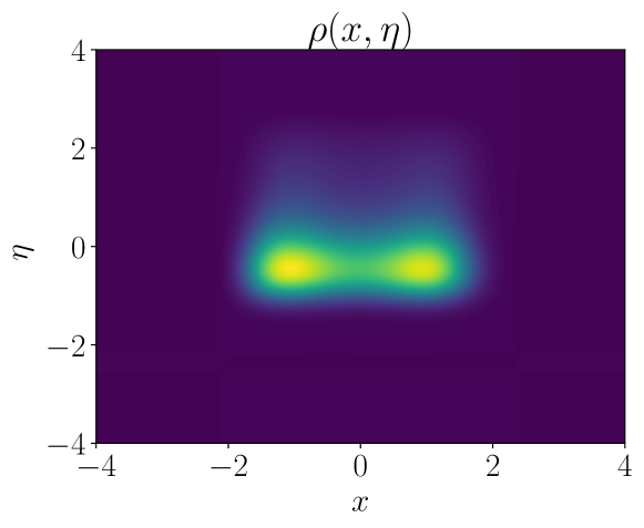
Refer to caption
(a) With the corrective drift.
Refer to caption
(b) Without the corrective drift.
Figure 6: Comparison of the numerical solutions for the steady-state Fokker–Planck equation when the noise is confined by potential (2.4), with and without the corrective drift term. Without correction, the parasitic drift completely deteriorates the accuracy of the solution.

We note however that, for fixed ε𝜀\varepsilon, μd0subscript𝜇𝑑0\mu_{d}\to 0 as d𝑑d\to\infty, by convergence of φ0,dsubscript𝜑0𝑑\varphi_{0,d} to CeVη𝐶superscriptesubscript𝑉𝜂C\,\operatorname{e}^{-V_{\eta}}. This is illustrated in fig. 7, where the same parameters as those used in fig. 6 were used. While the value of the bias decreases exponentially with the degree of approximation, we have found through numerical experiments that, when ε𝜀\varepsilon is of the order of 0.010.010.01, failure to account for the parasitic drift is very detrimental to the accuracy of the solution for d𝑑d as high as 30.

Refer to caption
Figure 7: Normalized bias εμd𝜀subscript𝜇𝑑\varepsilon\,\mu_{d} defined in (4.4), against degree of approximation, for ση2=0.1superscriptsubscript𝜎𝜂20.1\sigma_{\eta}^{2}=0.1. (The values shown need to be divided by ε𝜀\varepsilon to obtain the effective parasitic bias for a given value of ε𝜀\varepsilon.)

4.3 Numerical verification of the rates of convergence

In this section, we verify numerically the rate of convergence of the stationary solution to the Galerkin formulation eq. 3.11 in the limit ε0𝜀0\varepsilon\to 0. We recall that this Galerkin formulation is associated to the linear Fokker–Planck equation (3.11). In addition to verifying the rates of convergence, examining the limit ε0𝜀0\varepsilon\to 0 numerically will enable us to gain insight into the accuracy of the asymptotic expansions for moderate values of ε𝜀\varepsilon.

One-dimensional Ornstein–Uhlenbeck noise

For this test we use the same parameters as in the convergence study for the bistable potential in Subsection 3.3. We verify the accuracy of the asymptotic expansion up to order ε2superscript𝜀2\varepsilon^{2} of the full solution in the x𝑥xη𝜂\eta plane, given in [49, Chapter 3], by comparing it to numerical results obtained using the spectral method introduced in Section 3. The convergence is presented in fig. 8. We notice that, even for the smallest value of ε𝜀\varepsilon considered (26superscript262^{-6}), the norm of the difference between the asymptotic and spectral solutions appears to be roughly constant for d20𝑑20d\geq 20. This is because, beyond this point, the spectral method is more accurate than the asymptotic expansion.
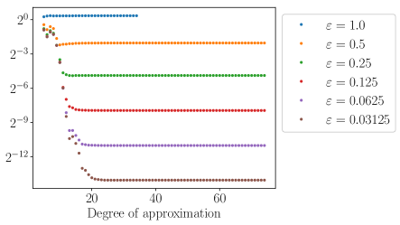
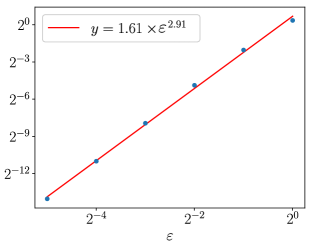
Refer to caption
Refer to caption
Figure 8: L1superscript𝐿1L^{1} norm of the difference between the solutions found using the Hermite spectral method and the asymptotic expansion up to order ε2superscript𝜀2\varepsilon^{2}, in both x𝑥x and η𝜂\eta, in the case of OU noise with ε=2i,i=0,,5formulae-sequence𝜀superscript2𝑖𝑖05\varepsilon=2^{-i},i=0,\dotsc,5 (left), and the corresponding L1superscript𝐿1L^{1} error of the asymptotic expansion (right). The scaling of the error (with respect to ε𝜀\varepsilon) is close to the expected value of 3.

Harmonic noise

The second case we consider is that of harmonic noise, for which the order of the first nontrival correction in the expansion of the solution is 𝒪(ε4)𝒪superscript𝜀4\mathcal{O}(\varepsilon^{4}); see [49]. We confirmed this numerically for V(x)=x4/4x2/2𝑉𝑥superscript𝑥44superscript𝑥22V(x)=x^{4}/4-x^{2}/2 and β=5𝛽5\beta=5 using 50 basis functions in each direction, with scaling factors σx2=1/30,σp2=σq2=1formulae-sequencesuperscriptsubscript𝜎𝑥2130superscriptsubscript𝜎𝑝2superscriptsubscript𝜎𝑞21\sigma_{x}^{2}=1/30,\sigma_{p}^{2}=\sigma_{q}^{2}=1. The results are illustrated in fig. 9.
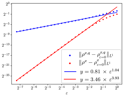
Refer to caption
Figure 9: Convergence as ε0𝜀0\varepsilon\to 0 in the case of harmonic noise. The observed rate of convergence of the x𝑥x-marginal to the white noise limit is 3.933.933.93, which is close to the theoretical value of 444. Here ρx,qsuperscript𝜌𝑥𝑞\rho^{x,q} denotes the marginal of the solution on the x,q𝑥𝑞x,q plane.

5 Results: effect of colored noise on bifurcations

In this section we present the bifurcation diagrams corresponding to the four models of the noise introduced in Section 2. We begin with the case of Gaussian noise, and later move to the case of non-Gaussian noise.

5.1 Construction of the bifurcation diagrams for the mean field equation

We constructed the bifurcation diagrams using three different approaches:

Monte Carlo simulations

We solved the system of interacting particles (2.1) with a sufficiently large number of particles, and we approximated the first moment by ergodic average over an interval (T,T+ΔT)𝑇𝑇Δ𝑇(T,T+\Delta T), where T𝑇T is sufficiently large to guarantee that the system has reached its stationary state and ΔTΔ𝑇\Delta T is sufficiently large to ensure that the ergodic averages are accurate. By applying this procedure for a range of inverse temperatures, β=0.1,0.15,0.2,,10𝛽0.10.150.210\beta=0.1,0.15,0.2,\dotsc,10, we obtained the desired bifurcation diagram.

Perturbation expansions

This approach, which we already outlined in Section 2, relies on the fact that the self-consistency map can be approximated as R(m,β)R0(m,β)+εδRδ(m,β)𝑅𝑚𝛽subscript𝑅0𝑚𝛽superscript𝜀𝛿subscript𝑅𝛿𝑚𝛽R(m,\beta)\approx R_{0}(m,\beta)+\varepsilon^{\delta}R_{\delta}(m,\beta), with good accuracy when ε1much-less-than𝜀1\varepsilon\ll 1. Here we used the same notation as in Section 2, and in particular δ𝛿\delta denotes the order of the first nontrivial correction in eq. 2.8. Using arclength continuation222We do this using the Moore–Penrose quasi-arclength continuation algorithm. The rigorous mathematical construction of the arclength continuation methodology can be found, e.g., in [30] and [3]. Some useful practical aspects of implementing arclength continuation are also given in [10]. See also [20]. for the resulting approximate self-consistency equation, m=R0(m,β)+εδRδ(m,β)𝑚subscript𝑅0𝑚𝛽superscript𝜀𝛿subscript𝑅𝛿𝑚𝛽m=R_{0}(m,\beta)+\varepsilon^{\delta}R_{\delta}(m,\beta), we can plot the first moment m𝑚m as a function of β𝛽\beta for a fixed value of ε𝜀\varepsilon. We note that, in view of the typical shape of the self-consistency map, depicted in a particular case in fig. 2, a standard root finding algorithm can be employed to initiate the arclength continuation at some initial inverse temperature β0subscript𝛽0\beta_{0}.

The spectral method

Finally, we employed the Galerkin method presented in Subsection 3.3. We considered two different methodologies: on the one hand, by calculating numerically an approximation ρd,(x,η;β,m)subscript𝜌𝑑𝑥𝜂𝛽𝑚\rho_{d,\infty}(x,\eta;\beta,m) of the steady-state solution of the linear Fokker–Planck equation (2.6a) with fixed m𝑚m and β𝛽\beta, we approximated the self-consistency map as R(m,β)𝐑𝐑nxρd,(x,η;β,m)dxd𝐲𝑅𝑚𝛽subscript𝐑subscriptsuperscript𝐑𝑛𝑥subscript𝜌𝑑𝑥𝜂𝛽𝑚differential-d𝑥differential-d𝐲R(m,\beta)\approx\int_{\mathbf{R}}\int_{\mathbf{R}^{n}}x\,\rho_{d,\infty}(x,\eta;\beta,m)\,\mathrm{d}x\,\mathrm{d}\boldsymbol{\mathbf{y}}, after which a bifurcation diagram can be constructed by using the same method as in the previous paragraph. Each evaluation of the self-consistency map requires the computation of the eigenvector associated with the eigenvalue of smallest magnitude of the discretized operator, which can be performed efficiently for sufficiently small systems using the SciPy toolbox. On the other hand, the time-dependent (nonlinear) McKean–Vlasov equation can be integrated directly using our spectral method. Since only the final solution is of interest to us, the semi-implicit time-stepping scheme (3.9) can be used with a large time step, which enables a quick and accurate approximation of the steady-state solutions. While both methodologies work well in the two-dimensional case, in three dimensions (harmonic noise) solving the McKean–Vlasov equation directly proved more efficient, so this is the approach we employed for all the tests presented in this section.

5.2 Gaussian case

The one-dimensional Ornstein–Uhlenbeck noise provides an ideal testbed for the three methods we use to construct bifurcation diagrams. Figure 10 below plots the bifurcation diagram of the first moment m𝑚m as a function of β𝛽\beta for ε=0.1,0.2,,0.5𝜀0.10.20.5\varepsilon=0.1,0.2,\dotsc,0.5. Three different initial conditions (𝐗0N(0,0.1),𝐗0N(0.1,0.1)formulae-sequencesimilar-tosubscript𝐗0𝑁00.1similar-tosubscript𝐗0𝑁0.10.1\boldsymbol{\mathbf{X}}_{0}\sim N(0,0.1),\,\boldsymbol{\mathbf{X}}_{0}\sim N(0.1,0.1), and 𝐗0N(0.1,0.1)similar-tosubscript𝐗0𝑁0.10.1\boldsymbol{\mathbf{X}}_{0}\sim N(-0.1,0.1)) were used for the MC simulations. Although we observe that the results of MC simulations tend to be less precise around the bifurcation point, the agreement between the three methods overall is excellent for ε=0.1,0.2𝜀0.10.2\varepsilon=0.1,0.2. For the other values of ε𝜀\varepsilon, while the results of MC simulations and of our spectral method continue to agree, those obtained from the asymptotic expansion are significantly less accurate, which is consistent with the observations presented in fig. 8.
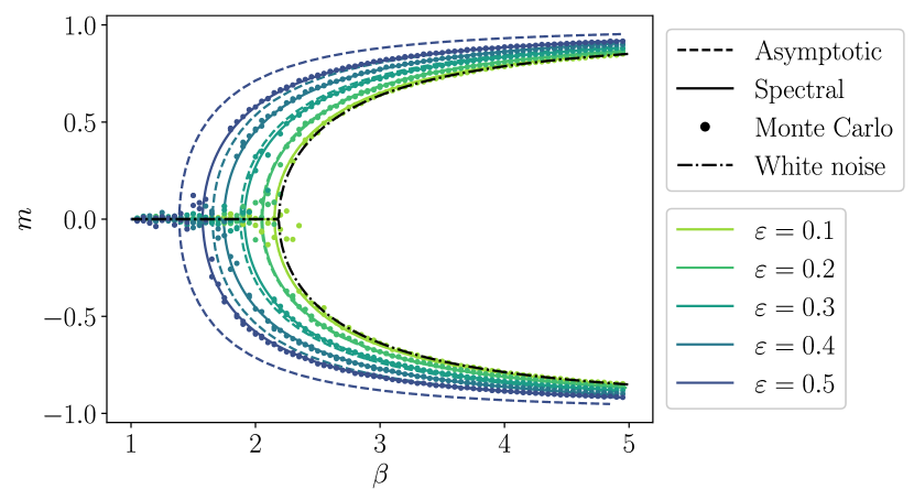
Refer to caption
Figure 10: Bifurcation diagram of m𝑚m against β𝛽\beta for Ornstein–Uhlenbeck noise, obtained via MC simulation, the spectral method, and the asymptotic expansion (2.9).

The case of harmonic noise, corresponding to a three-dimensional McKean–Vlasov equation, is more challenging to tackle using our spectral method. When using 40 basis functions in each direction, the CPU time required to construct the full bifurcation diagram was of the order of a week. As a consequence of the lower number of basis functions used in this case, we observe a small discrepancy between the results of the spectral method and those of MC simulations for large β𝛽\beta in the case ε=0.4𝜀0.4\varepsilon=0.4. Nevertheless, as can be seen in fig. 11, for small ε𝜀\varepsilon the overall agreement between the three methods is excellent. We note in particular that, as suggested by the asymptotic expansions, the use of harmonic noise produces results much closer to the white noise limit than scalar OU noise.
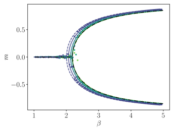
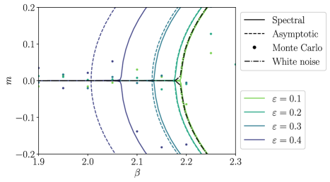
Refer to caption
Refer to caption
Figure 11: Bifurcation diagram of m𝑚m against β𝛽\beta for harmonic noise (model H), obtained via MC simulation, the Hermite spectral method, and the asymptotic expansion (2.9).

5.3 Non-Gaussian noise

For the non-Gaussian noise processes we consider, the x4superscript𝑥4x^{4} asymptotic growth of the confining potentials in both directions causes the McKean–Vlasov equation to be stiffer than in the cases of OU and harmonic noise, especially for large values of ε𝜀\varepsilon. Consequently, we were not able to consider as wide a range of ε𝜀\varepsilon as in the previous subsection using the spectral method. Since, on the other hand, MC simulations become overly computationally expensive for small ε𝜀\varepsilon, the comparisons in this section comprise only results obtained using our spectral method and asymptotic expansions. Results of simulations for the bistable noise (model B) are presented in fig. 12, in which a very good agreement can be observed.
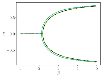
Refer to caption
Refer to caption
Figure 12: Bifurcation diagram of m𝑚m against β𝛽\beta for the bistable noise (model B), using the spectral method and a truncated asymptotic expansion including the first nonzero correction. We see that, overall, the agreement between the two methods is excellent.

For nonsymmetric noise (model NS), the two branches in the bifurcation diagram are separate, as illustrated in fig. 13. Here too, the agreement between the spectral method and the asymptotic expansion is excellent. In contrast with the other models considered, the first nonzero term in the asymptotic expansion is of order ε𝜀\varepsilon, which is reflected by the manifestly higher sensitivity to the correlation time of the noise. In the right panel of fig. 13, we present the graph of R0(m;β)+εR1(m;β)subscript𝑅0𝑚𝛽𝜀subscript𝑅1𝑚𝛽R_{0}(m;\beta)+\varepsilon R_{1}(m;\beta) for a value of β𝛽\beta close to the point at which new branches (one stable and one unstable) emerge.
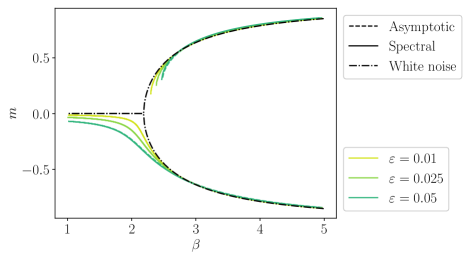
Refer to caption
Refer to caption
Figure 13: Left: bifurcation diagram of m𝑚m against β𝛽\beta for the nonsymmetric noise (model NS), using the spectral method and a truncated asymptotic expansion including the first nonzero correction. Right: R0+εR1(m)msubscript𝑅0𝜀subscript𝑅1𝑚𝑚R_{0}+\varepsilon R_{1}(m)-m against m𝑚m for ε=0.1𝜀0.1\varepsilon=0.1 and β=2.6𝛽2.6\beta=2.6.

5.4 Dependence of the critical temperature on ε𝜀\varepsilon

For the noise models OU, H and B, the effect of colored noise on the dynamics is a shift of the critical temperature: the pitchfork bifurcation occurs for smaller values of β𝛽\beta (i.e., larger temperatures) as the correlation time increases. In order to further investigate the effect of the correlation time on the long time behavior of the system of interacting particles, we will compute the critical temperature as a function of ε𝜀\varepsilon based on the asymptotic expansions and compare with the results of spectral and MC simulations, see fig. 14. Rather than finding the critical inverse temperature βCsubscript𝛽𝐶\beta_{C} for a range of values of ε𝜀\varepsilon (and for a fixed θ𝜃\theta), it is convenient to fix βCsubscript𝛽𝐶\beta_{C} and find the corresponding ε𝜀\varepsilon, satisfying

ddm(𝐑xp0(x;βC,m)dx)m=0+εδddm(𝐑pδ(x;βC,m)dx)m=0=1,dd𝑚subscriptsubscript𝐑𝑥subscript𝑝0𝑥subscript𝛽𝐶𝑚differential-d𝑥𝑚0superscript𝜀𝛿dd𝑚subscriptsubscript𝐑subscript𝑝𝛿𝑥subscript𝛽𝐶𝑚differential-d𝑥𝑚01\mathchoice{\frac{\mathrm{d}{}}{\mathrm{d}m}}{\mathrm{d}_{m}}{}{}\left(\int_{\mathbf{R}}x\,p_{0}(x;\beta_{C},m)\,\mathrm{d}x\right)_{m=0}+\varepsilon^{\delta}\mathchoice{\frac{\mathrm{d}{}}{\mathrm{d}m}}{\mathrm{d}_{m}}{}{}\left(\int_{\mathbf{R}}p_{\delta}(x;\beta_{C},m)\,\mathrm{d}x\right)_{m=0}=1, (5.1)

which is merely a polynomial equation in ε𝜀\varepsilon, the coefficient of which can be calculated by numerical differentiation. With this procedure, the dependence of the critical β𝛽\beta upon ε𝜀\varepsilon can be calculated on a fine mesh. In the case of OU noise, for example, both coefficients on the left-hand side of eq. 5.1 are positive, implying that the equation has a solution (in fact, two, but one of them negative) only if βCsubscript𝛽𝐶\beta_{C} is lower than the inverse critical temperature in the white noise case.

Of the three methods employed in fig. 14, the approach based on the asymptotic expansions has the lowest computational cost: calculating all the solid curves took only about a couple of minutes on a personal computer with an Intel i7-3770 processor. The data points associated with the spectral method and the MC simulations were obtained from the bifurcation diagrams presented above.
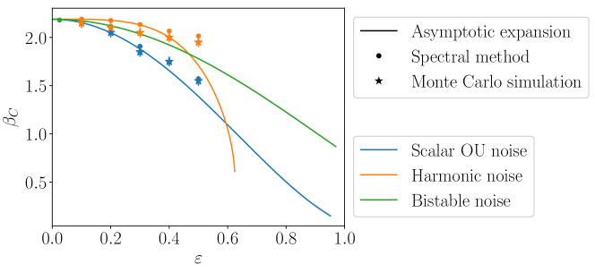
Refer to caption
Figure 14: Critical β𝛽\beta against ε𝜀\varepsilon.

6 Conclusions

In this paper, we introduced a robust spectral method for the numerical solution of linear and nonlinear, local and nonlocal Fokker–Planck-type PDEs that does not require that the PDE is a gradient flow. We then used our method to construct the bifurcation diagram for the stationary solutions of the mean field limit of a system of weakly interacting particles driven by colored noise.

To verify our results, we also constructed the bifurcation diagrams by using two other independent approaches, namely by MC simulation of the N𝑁N-particle system and by using explicit asymptotic expansions with respect to correlation time of the noise. In the small correlation time regime, we observed a very good agreement between all three methods. For larger values of the correlation time, the asymptotic expansions become inaccurate, but the results obtained via the spectral method and MC simulations continue to be in good agreement.

It appeared from our study that, unless the potential in which the noise process is confined is asymmetric, the correlation structure of the noise does not influence the topology of the bifurcation diagram: the mean-zero steady-state solution, which is stable for sufficiently large temperatures, becomes unstable as the temperature decreases below a critical value, at which point two new stable branches emerge, in the same manner as reported in [9, 44]. The correlation structure does, however, influence the temperature at which bifurcation occurs, and in general this temperature increases as the correlation time of the noise increases. In the presence of an asymmetry in the confining potential of the noise, on the other hand, the two stable branches in the bifurcation diagram are separate, indicating that the system always reaches the same equilibrium upon slowly decreasing the temperature. This behavior is similar to what has been observed previously in the white noise case when a tilt is introduced in the confining potential V()𝑉V(\cdot), see [20, 21].

Several problems remain open for future work. On the theoretical front, we believe that the analysis we presented in Subsections 3.1 and B for the linear Fokker–Planck equation can be extended to both the linear Fokker–Planck equation with colored noise and the nonlinear McKean–Vlasov equation. Another direction for future research could be the rigorous study of bifurcations and, more specifically, of fluctuations and critical slowing down near the bifurcation point. On the modeling front, it would be interesting to consider more general evolution equations for the interacting particles, such as the generalized Langevin equation, and also to study systems of interacting particles subject to colored noise that is multiplicative.

Appendix A Hermite polynomials and Hermite functions

In one dimension, the orthonormal Hermite polynomials can be defined by:

Hn(x)=(1)nn!exp(x22)dndxn(exp(x22)),n=0,1,formulae-sequencesubscript𝐻𝑛𝑥superscript1𝑛𝑛superscript𝑥22superscriptd𝑛dsuperscript𝑥𝑛superscript𝑥22𝑛01H_{n}(x)=\frac{(-1)^{n}}{\sqrt{n!}}\exp\left({\frac{x^{2}}{2}}\right)\mathchoice{\frac{\mathrm{d}^{n}{}}{\mathrm{d}x^{n}}}{\mathrm{d}_{x}^{n}}{}{}\,\left(\exp{\left(-\frac{x^{2}}{2}\right)}\right),\qquad n=0,1,\dotsc

They form a complete orthonormal basis of the weighted space L2(𝐑;g)superscript𝐿2𝐑𝑔L^{2}(\mathbf{R};g), where g:=ex2/2/2πassign𝑔superscriptesuperscript𝑥222𝜋g:=\operatorname{e}^{-x^{2}/2}/\sqrt{2\,\pi}, and they satisfy the following recursion relations (eq. A.3 can be obtained by combining eqs. A.1 and A.2):

(xddx)Hn=n+1Hn+1;𝑥dd𝑥subscript𝐻𝑛𝑛1subscript𝐻𝑛1\displaystyle\left(x-\mathchoice{\frac{\mathrm{d}{}}{\mathrm{d}x}}{\mathrm{d}_{x}}{}{}\right)\,H_{n}=\sqrt{n+1}\,H_{n+1}; (A.1)
Hn+1=i=0nHi𝐑Hn+1Hi(x)g(x)dx=n+1Hn;superscriptsubscript𝐻𝑛1subscriptsuperscript𝑛𝑖0subscript𝐻𝑖subscript𝐑superscriptsubscript𝐻𝑛1subscript𝐻𝑖𝑥𝑔𝑥differential-d𝑥𝑛1subscript𝐻𝑛\displaystyle H_{n+1}^{\prime}=\sum^{n}_{i=0}\,H_{i}\,\int_{\mathbf{R}}H_{n+1}^{\prime}\,H_{i}(x)\,g(x)\,\mathrm{d}x=\sqrt{n+1}\,H_{n}; (A.2)
Hn+1=1n+1xHnnn+1Hn1.subscript𝐻𝑛11𝑛1𝑥subscript𝐻𝑛𝑛𝑛1subscript𝐻𝑛1\displaystyle H_{n+1}=\sqrt{\frac{1}{n+1}}\,x\,H_{n}-\sqrt{\frac{n}{n+1}}H_{n-1}. (A.3)

From eqs. A.1 and A.2, we see that Hermite polynomials are the eigenfunctions of a second-order operator:

Hi:=xxHi:=(xddx)ddxHi=iHi,assignsubscript𝐻𝑖subscriptsuperscript𝑥subscript𝑥subscript𝐻𝑖assign𝑥dd𝑥dd𝑥subscript𝐻𝑖𝑖subscript𝐻𝑖\mathcal{L}\,H_{i}:=\partial^{*}_{x}\partial_{x}\,H_{i}:=\left(x-\mathchoice{\frac{\mathrm{d}{}}{\mathrm{d}x}}{\mathrm{d}_{x}}{}{}\right)\mathchoice{\frac{\mathrm{d}{}}{\mathrm{d}x}}{\mathrm{d}_{x}}{}{}H_{i}=i\,H_{i}, (A.4)

which is essential to proving approximation results. We note that the eigenvalues grow linearly, which explains the square root in the rate of convergence in the results presented below. Since Hermite polynomials constitute an orthonormal basis of L2(𝐑;g)superscript𝐿2𝐑𝑔L^{2}(\mathbf{R};g), any function u𝑢u in that space can be expanded as a series of Hermite polynomials, and

i=0dHiu,HiguinL2(𝐑;g)asd.formulae-sequencesuperscriptsubscript𝑖0𝑑subscript𝐻𝑖subscript𝑢subscript𝐻𝑖𝑔𝑢insuperscript𝐿2𝐑𝑔as𝑑\sum_{i=0}^{d}H_{i}\,\left\langle{u,H_{i}}\right\rangle_{g}\to u\quad\text{in}~{}L^{2}(\mathbf{R};g)~{}\text{as}~{}d\to\infty.

We will call Hermite transform the operator:

𝒯::𝒯absent\displaystyle\mathcal{T}:\, L2(𝐑;g)2superscript𝐿2𝐑𝑔superscript2\displaystyle L^{2}(\mathbf{R};g)\to\ell^{2}
u(u,H0g,u,H1g,).maps-to𝑢subscript𝑢subscript𝐻0𝑔subscript𝑢subscript𝐻1𝑔\displaystyle u\mapsto\big{(}\left\langle{u,H_{0}}\right\rangle_{g},\left\langle{u,H_{1}}\right\rangle_{g},\dotsc\big{)}.

Denoting by ΠdsubscriptΠ𝑑\Pi_{d} the L2(𝐑;g)superscript𝐿2𝐑𝑔L^{2}(\mathbf{R};g) projection operator on span{H0,H1,,Hd}spansubscript𝐻0subscript𝐻1subscript𝐻𝑑\operatorname{span}\{H_{0},H_{1},\dotsc,H_{d}\}, the following theorem follows from (A.2); see [43] for details.

Theorem A.1 (Approximation by Hermite polynomials).

For any uHm(𝐑;g)𝑢superscript𝐻𝑚𝐑𝑔u\in H^{m}(\mathbf{R};g) with 0md+10𝑚𝑑10\leq m\leq d+1, the following inequality holds:

ddx(Πduu)g(dm+1)!(d+1)!u(m)g,=0,,m.formulae-sequencesubscriptnormsuperscriptddsuperscript𝑥subscriptΠ𝑑𝑢𝑢𝑔𝑑𝑚1𝑑1subscriptnormsuperscript𝑢𝑚𝑔0𝑚\left\|\mathchoice{\frac{\mathrm{d}^{\ell}{}}{\mathrm{d}x^{\ell}}}{\mathrm{d}_{x}^{\ell}}{}{}(\Pi_{d}u-u)\right\|_{g}\leq\sqrt{\frac{(d-m+1)!}{(d-\ell+1)!}}\,\|u^{(m)}\|_{g},\qquad\ell=0,\dotsc,m.

The Hermite polynomials, as defined above, are suitable for the approximation of functions with respect to the norm of L2(𝐑;g)superscript𝐿2𝐑𝑔L^{2}(\mathbf{R};g), which assigns a significant weight only to the region around x=0𝑥0x=0. For the approximation with respect to the flat L2(𝐑)superscript𝐿2𝐑L^{2}(\mathbf{R}) norm, or with respect to other norms that penalize growth as x𝑥x\to\infty, such as the weighted L2(𝐑;ex2/2)superscript𝐿2𝐑superscript𝑒superscript𝑥22L^{2}(\mathbf{R};e^{x^{2}/2}) norm, one can use the basis functions (eU/2Hi)i=0superscriptsubscriptsuperscripte𝑈2subscript𝐻𝑖𝑖0(\operatorname{e}^{-U/2}\,H_{i})_{i=0}^{\infty} for some function U𝑈U, which constitute an orthonormal basis of L2(𝐑n;eUg)superscript𝐿2superscript𝐑𝑛superscripte𝑈𝑔L^{2}(\mathbf{R}^{n};\operatorname{e}^{U}g). For uL2(𝐑;eUg)𝑢superscript𝐿2𝐑superscripte𝑈𝑔u\in L^{2}(\mathbf{R};\operatorname{e}^{U}g), we define the generalized Hermite transform associated with the factor eU/2superscripte𝑈2\operatorname{e}^{-U/2}, which we denote by 𝒯Usubscript𝒯𝑈\mathcal{T}_{U}:

𝒯U::subscript𝒯𝑈absent\displaystyle\mathcal{T}_{U}: L2(𝐑;eUg)2superscript𝐿2𝐑superscripte𝑈𝑔superscript2\displaystyle L^{2}(\mathbf{R};\operatorname{e}^{U}g)\to\ell^{2} (A.5)
u(u,eU/2H0eUg,u,eU/2H1eUg,).maps-to𝑢subscript𝑢superscripte𝑈2subscript𝐻0superscripte𝑈𝑔subscript𝑢superscripte𝑈2subscript𝐻1superscripte𝑈𝑔\displaystyle u\mapsto\left(\left\langle{u,\operatorname{e}^{-U/2}H_{0}}\right\rangle_{\operatorname{e}^{U}g},\left\langle{u,\operatorname{e}^{-U/2}H_{1}}\right\rangle_{\operatorname{e}^{U}g},\dotsc\right).

Note that 𝒯U(u)=𝒯(eU/2u)subscript𝒯𝑈𝑢𝒯superscripte𝑈2𝑢\mathcal{T}_{U}(u)=\mathcal{T}(\operatorname{e}^{U/2}u), i.e. TU(u)subscript𝑇𝑈𝑢T_{U}(u) is the usual Hermite transform of eU/2usuperscripte𝑈2𝑢\operatorname{e}^{U/2}u. This formalism enables us to treat in a unified manner the case of Hermite polynomials (U=0𝑈0U=0), of Hermite functions (eU/2=gsuperscripte𝑈2𝑔\operatorname{e}^{-U/2}=\sqrt{g}), as well as other useful cases. As an example of why such generality can be useful, it has been shown in [14] that the choice eU/2=gsuperscripte𝑈2𝑔\operatorname{e}^{-U/2}=g leads to basis functions, referred to as generalized Hermite functions in that paper, that can be used to design an efficient numerical method for the solution of the Kramers Fokker–Planck equation. By the property (A.4), we see that (eU/2Hi)i=0superscriptsubscriptsuperscripte𝑈2subscript𝐻𝑖𝑖0(\operatorname{e}^{-U/2}H_{i})_{i=0}^{\infty} are the eigenfunctions of the operator:

u(eU/2eU/2)u,maps-to𝑢superscripte𝑈2superscripte𝑈2𝑢u\mapsto(\operatorname{e}^{-U/2}\mathcal{L}\operatorname{e}^{U/2})u,

which is of Schrödinger type when eU=gsuperscripte𝑈𝑔\operatorname{e}^{-U}=g, see [39]. Introducing the notations ΠdU:=eU/2ΠdeU/2assignsuperscriptsubscriptΠ𝑑𝑈superscripte𝑈2subscriptΠ𝑑superscripte𝑈2\Pi_{d}^{U}:=\operatorname{e}^{-U/2}\Pi_{d}\operatorname{e}^{U/2} and xU:=x+U/2=eU/2x(eU/2)\partial_{x}^{U}:=\partial_{x}+U^{\prime}/2=\operatorname{e}^{-U/2}\partial_{x}(\operatorname{e}^{U/2}\cdot), we have the following immediate corollary of theorem A.1.

Corollary A.2 (Approximation by generalized Hermite functions).

For any u𝑢u such that (xU)muL2(𝐑;eUg)superscriptsuperscriptsubscript𝑥𝑈𝑚𝑢superscript𝐿2𝐑superscripte𝑈𝑔(\partial_{x}^{U})^{m}u\in L^{2}(\mathbf{R};\operatorname{e}^{U}g) with 0md+10𝑚𝑑10\leq m\leq d+1,

(xU)(ΠdUuu)eUg(dm+1)!(d+1)!(xU)mueUg,=0,,m.formulae-sequencesubscriptnormsuperscriptsuperscriptsubscript𝑥𝑈superscriptsubscriptΠ𝑑𝑈𝑢𝑢superscripte𝑈𝑔𝑑𝑚1𝑑1subscriptnormsuperscriptsuperscriptsubscript𝑥𝑈𝑚𝑢superscripte𝑈𝑔0𝑚\|(\partial_{x}^{U})^{\ell}(\Pi_{d}^{U}u-u)\|_{\operatorname{e}^{U}g}\leq\sqrt{\frac{(d-m+1)!}{(d-\ell+1)!}}\,\|(\partial_{x}^{U})^{m}u\|_{\operatorname{e}^{U}g},\qquad\ell=0,\dotsc,m.

In the case eU=gsuperscripte𝑈𝑔\operatorname{e}^{-U}=g (orthonormal Hermite functions in L2(𝐑)superscript𝐿2𝐑L^{2}(\mathbf{R})), one can prove a similar statement with the usual derivative instead of xUsuperscriptsubscript𝑥𝑈\partial_{x}^{U} in the left-hand side, see [43, Theorem 7.14]. We note that theorems A.1 and A.2 can be extended to the multi-dimensional case, see e.g. [1].

In addition to the function eU/2superscripte𝑈2\operatorname{e}^{-U/2} multiplying the Hermite polynomials in the definition of basis functions, it is usual in numerical simulations to introduce a scaling factor, which can be chosen appropriately depending on how localized the function to be approximated is. We define Hiσ(x):=Hi(x/σ)assignsubscriptsuperscript𝐻𝜎𝑖𝑥subscript𝐻𝑖𝑥𝜎H^{\sigma}_{i}(x):=H_{i}(x/\sigma), and note that these polynomials form an orthonormal basis in L2(𝐑;gσ)superscript𝐿2𝐑subscript𝑔𝜎L^{2}(\mathbf{R};g_{\sigma}), where gσsubscript𝑔𝜎g_{\sigma} is the normal distribution with mean 0 and variance σ2superscript𝜎2\sigma^{2}. Although we do not present them explicitly, approximation results similar to theorems A.1 and A.2 can be proved in the presence of this scaling factor, with the only difference being the presence of additional constant factors on the right-hand side; see, for example, [1].

The importance of choosing this scaling factor in a suitable manner was demonstrated rigorously in [46], where the author shows that, for Gaussian-type functions, the optimal value of σ𝜎\sigma should depend on the number of basis function used with a dependence of the form 1/d1𝑑1/\sqrt{d}. This can be justified intuitively by taking into account that, on the one hand, the behavior of Hermite functions as x𝑥x\to\infty is well-understood, with the final inflection point occurring at xdσproportional-to𝑥𝑑𝜎x\propto\sqrt{d}\,\sigma and a rapid decrease to 0 beyond that point [31], and that, on the other hand, scaled Hermite functions are eigenfunctions of the Fourier transform operator, up to dilations/contractions. Since a contraction in real space results in a dilation in Fourier space, by choosing a scaling factor that decreases with d𝑑d one effectively favors exploration in Fourier space. In particular, choosing σ1/dproportional-to𝜎1𝑑\sigma\propto 1/\sqrt{d} leads to a situation where the position of the final inflection point of the Hermite function of highest order remains approximately constant (while the position of the final inflection point of its Fourier transform grows linearly), so it is crucial in that case to ensure that dσ𝑑𝜎\sqrt{d}\,\sigma is large enough to ensure that the basis functions cover the support of the target function.

In practice, calculating the Hermite transform numerically requires the introduction of a quadrature. To bound the associated error, results similar to theorems A.1 and A.2, with the projection operators replaced by interpolation operators, can be proved; see [43, Theorems 7.17, 7.18].

Appendix B Proof of theorem 3.1

Using the same notation as in appendix A, we let ΠdsubscriptΠ𝑑\Pi_{d} be the L2(𝐑;eVq)superscript𝐿2𝐑superscript𝑒subscript𝑉𝑞L^{2}(\mathbf{R};e^{-V_{q}}) projection operator on 𝐏(d)𝐏𝑑\mathbf{P}(d) and Π^d:=eVq/2ΠdeVq/2assignsubscript^Π𝑑superscript𝑒subscript𝑉𝑞2subscriptΠ𝑑superscript𝑒subscript𝑉𝑞2\hat{\Pi}_{d}:=e^{-V_{q}/2}\,\Pi_{d}\,e^{V_{q}/2}. The solution udsubscript𝑢𝑑u_{d} of eq. 3.3a satisfies tud=Π^dxΠ^dud=:dud\partial_{t}u_{d}=\hat{\Pi}_{d}\,\mathcal{H}_{x}\,\hat{\Pi}_{d}\,u_{d}=:\mathcal{H}_{d}\,u_{d}. Clearly, the operator dsubscript𝑑\mathcal{H}_{d} is selfadjoint on eVq/2𝐏(d)superscriptesubscript𝑉𝑞2𝐏𝑑\operatorname{e}^{-V_{q}/2}\mathbf{P}(d) with the L2(𝐑)superscript𝐿2𝐑L^{2}(\mathbf{R}) inner product, and it is also negative, by negativity of xsubscript𝑥\mathcal{H}_{x}:

dwd,wd=xwd,wd0wdeVq/2𝐏(d).formulae-sequencesubscript𝑑subscript𝑤𝑑subscript𝑤𝑑subscript𝑥subscript𝑤𝑑subscript𝑤𝑑0for-allsubscript𝑤𝑑superscriptesubscript𝑉𝑞2𝐏𝑑\left\langle{\mathcal{H}_{d}w_{d},w_{d}}\right\rangle=\left\langle{\mathcal{H}_{x}w_{d},w_{d}}\right\rangle\leq 0\quad\forall w_{d}\in\operatorname{e}^{-V_{q}/2}\mathbf{P}(d). (B.1)

To prove the convergence of udsubscript𝑢𝑑u_{d} when d𝑑d\to\infty, we will rely on the following lemma.

Lemma B.1.

Let ^x:=x+x/2assignsubscript^𝑥subscript𝑥𝑥2\hat{\partial}_{x}:=\partial_{x}+x/2, and assume that ^xnuL2(𝐑)superscriptsubscript^𝑥𝑛𝑢superscript𝐿2𝐑\hat{\partial}_{x}^{n}u\in L^{2}(\mathbf{R}) for n=0,,m𝑛0𝑚n=0,\dots,m. Then for all natural numbers m1,m2subscript𝑚1subscript𝑚2m_{1},m_{2} such that m1+m2msubscript𝑚1subscript𝑚2𝑚m_{1}+m_{2}\leq m, it holds that xm1u(m2)L2(𝐑)superscript𝑥subscript𝑚1superscript𝑢subscript𝑚2superscript𝐿2𝐑x^{m_{1}}\,u^{(m_{2})}\in L^{2}(\mathbf{R}) and

K1(m)maxm1+m2mxm1u(m2)max0im^xiuK2(m)maxm1+m2mxm1u(m2),subscript𝐾1𝑚subscriptsubscript𝑚1subscript𝑚2𝑚normsuperscript𝑥subscript𝑚1superscript𝑢subscript𝑚2subscript0𝑖𝑚normsuperscriptsubscript^𝑥𝑖𝑢subscript𝐾2𝑚subscriptsubscript𝑚1subscript𝑚2𝑚normsuperscript𝑥subscript𝑚1superscript𝑢subscript𝑚2\displaystyle K_{1}(m)\,\max_{m_{1}+m_{2}\leq m}\,\|x^{m_{1}}\,u^{(m_{2})}\|\leq\max_{0\leq i\leq m}\|\hat{\partial}_{x}^{i}u\|\leq K_{2}(m)\,\max_{m_{1}+m_{2}\leq m}\,\|x^{m_{1}}\,u^{(m_{2})}\|, (B.2)

where K1(m),K2(m)subscript𝐾1𝑚subscript𝐾2𝑚K_{1}(m),K_{2}(m) are positive constants depending only on m𝑚m and \|\cdot\| is the usual L2(𝐑)superscript𝐿2𝐑L^{2}(\mathbf{R}) norm.

Proof.

We denote by Hm(𝐑;ex2/2)superscript𝐻𝑚𝐑superscriptesuperscript𝑥22H^{m}(\mathbf{R};\operatorname{e}^{-x^{2}/2}) the Sobolev space weighted by ex2/2superscriptesuperscript𝑥22\operatorname{e}^{-x^{2}/2},

Hm(𝐑;ex2/2)={v:v(i)L2(𝐑;ex2/2) for i=0,,m},superscript𝐻𝑚𝐑superscriptesuperscript𝑥22conditional-set𝑣formulae-sequencesuperscript𝑣𝑖superscript𝐿2𝐑superscriptesuperscript𝑥22 for 𝑖0𝑚H^{m}(\mathbf{R};\operatorname{e}^{-x^{2}/2})=\{v:v^{(i)}\in L^{2}(\mathbf{R};\operatorname{e}^{-x^{2}/2})\text{ for }i=0,\dotsc,m\},

and by m,ex2/2\|\cdot\|_{m,\operatorname{e}^{-x^{2}/2}} the associated norm: vm,ex2/22=i=0mv(i)ex2/22superscriptsubscriptnorm𝑣𝑚superscriptesuperscript𝑥222superscriptsubscript𝑖0𝑚superscriptsubscriptnormsuperscript𝑣𝑖superscriptesuperscript𝑥222\|v\|_{m,\operatorname{e}^{-x^{2}/2}}^{2}=\sum_{i=0}^{m}\|v^{(i)}\|_{\operatorname{e}^{-x^{2}/2}}^{2}. For the first inequality, we know from [43, Lemma B.6] that

xvex2/24v1,ex2/2vH1(𝐑;ex2/2).formulae-sequencesubscriptnorm𝑥𝑣superscriptesuperscript𝑥224subscriptnorm𝑣1superscriptesuperscript𝑥22for-all𝑣superscript𝐻1𝐑superscriptesuperscript𝑥22\|xv\|_{\operatorname{e}^{-x^{2}/2}}\leq 4\,\|v\|_{1,\operatorname{e}^{-x^{2}/2}}\qquad\forall v\in H^{1}(\mathbf{R};\operatorname{e}^{-x^{2}/2}).

Applying this inequality repeatedly, we obtain

xm1vex2/2C(m)vm,ex2/2,m1=0,,m,vHm(𝐑;ex2/2),formulae-sequencesubscriptnormsuperscript𝑥subscript𝑚1𝑣superscriptesuperscript𝑥22𝐶𝑚subscriptnorm𝑣𝑚superscriptesuperscript𝑥22formulae-sequencesubscript𝑚10𝑚for-all𝑣superscript𝐻𝑚𝐑superscriptesuperscript𝑥22\displaystyle\|x^{m_{1}}v\|_{\operatorname{e}^{-x^{2}/2}}\leq C(m)\,\|v\|_{m,\operatorname{e}^{-x^{2}/2}},\qquad m_{1}=0,\dotsc,m,\qquad\forall v\in H^{m}(\mathbf{R};\operatorname{e}^{-x^{2}/2}), (B.3)

for a constant C(m)𝐶𝑚C(m) depending only on m𝑚m. By definition, ^xu=ex2/4x(ex2/4u)subscript^𝑥𝑢superscriptesuperscript𝑥24subscript𝑥superscriptesuperscript𝑥24𝑢\hat{\partial}_{x}u=\operatorname{e}^{-x^{2}/4}\partial_{x}(\operatorname{e}^{x^{2}/4}u), so the assumption implies that ex2/4uHm(𝐑;ex2/2)superscriptesuperscript𝑥24𝑢superscript𝐻𝑚𝐑superscriptesuperscript𝑥22\operatorname{e}^{x^{2}/4}u\in H^{m}(\mathbf{R};\operatorname{e}^{-x^{2}/2}), from which we obtain using eq. B.3 that, for 0m1m0subscript𝑚1𝑚0\leq m_{1}\leq m,

xm1u=xm1uex2/4ex2/2C(m)uex2/4m,ex2/2=C(m)i=0m^xmu2.normsuperscript𝑥subscript𝑚1𝑢subscriptnormsuperscript𝑥subscript𝑚1𝑢superscriptesuperscript𝑥24superscriptesuperscript𝑥22𝐶𝑚subscriptnorm𝑢superscriptesuperscript𝑥24𝑚superscriptesuperscript𝑥22𝐶𝑚superscriptsubscript𝑖0𝑚superscriptnormsuperscriptsubscript^𝑥𝑚𝑢2\|x^{m_{1}}u\|=\|x^{m_{1}}u\,\operatorname{e}^{x^{2}/4}\|_{\operatorname{e}^{-x^{2}/2}}\leq C(m)\,\|u\,\operatorname{e}^{x^{2}/4}\|_{m,\operatorname{e}^{-x^{2}/2}}=C(m)\sqrt{\sum_{i=0}^{m}\|\hat{\partial}_{x}^{m}u\|^{2}}.

This proves the first inequality of eq. B.2 in the case m2=0subscript𝑚20m_{2}=0. We assume now that the statement is proved up to m21subscript𝑚21m_{2}-1, and we show that it is valid for m2subscript𝑚2m_{2}. Using the triangle inequality we obtain

xm1u(m2)xm1(u(m2)^xm2u)+xm1^xm2u.normsuperscript𝑥subscript𝑚1superscript𝑢subscript𝑚2normsuperscript𝑥subscript𝑚1superscript𝑢subscript𝑚2superscriptsubscript^𝑥subscript𝑚2𝑢normsuperscript𝑥subscript𝑚1superscriptsubscript^𝑥subscript𝑚2𝑢\displaystyle\|x^{m_{1}}\,u^{(m_{2})}\|\leq\|x^{m_{1}}\,(u^{(m_{2})}-\hat{\partial}_{x}^{m_{2}}u)\|+\|x^{m_{1}}\,\hat{\partial}_{x}^{m_{2}}u\|.

The derivatives in the first term are of order strictly lower than m2subscript𝑚2m_{2}, and therefore this term can be bounded by the induction assumption. The second term is bounded by applying the base case to ^xm2usuperscriptsubscript^𝑥subscript𝑚2𝑢\hat{\partial}_{x}^{m_{2}}u: introducing v:=^xm2uassign𝑣superscriptsubscript^𝑥subscript𝑚2𝑢v:=\hat{\partial}_{x}^{m_{2}}u, we notice that ^xmm2v=^xmuL2(𝐑)superscriptsubscript^𝑥𝑚subscript𝑚2𝑣superscriptsubscript^𝑥𝑚𝑢superscript𝐿2𝐑\hat{\partial}_{x}^{m-m_{2}}v=\hat{\partial}_{x}^{m}u\in L^{2}(\mathbf{R}) by assumption, so we can apply the first inequality in eq. B.2, without any derivative of v𝑣v in the left-hand side, to deduce

xmm2vmax0imm2^xivmax0im^xiu.normsuperscript𝑥𝑚subscript𝑚2𝑣subscript0𝑖𝑚subscript𝑚2normsuperscriptsubscript^𝑥𝑖𝑣subscript0𝑖𝑚normsuperscriptsubscript^𝑥𝑖𝑢\|x^{m-m_{2}}v\|\leq\max_{0\leq i\leq m-m_{2}}\|\hat{\partial}_{x}^{i}v\|\leq\max_{0\leq i\leq m}\|\hat{\partial}_{x}^{i}u\|.

The second inequality in (B.2) then holds trivially by expanding ^xsubscript^𝑥\hat{\partial}_{x} and applying a triangle inequality. ∎

With 3.1, we can show that the two norms in lemma B.1 can be bounded from above by the norm (x+1)mu,usuperscriptsubscript𝑥1𝑚𝑢𝑢\sqrt{\left\langle{{(-\mathcal{H}_{x}+1)}^{m}u,u}\right\rangle} for appropriate m𝑚m.

Lemma B.2 (Bound by alternative norm).

If 3.1 holds, then

i=0m^xmu2C(x+1)mu,usuperscriptsubscript𝑖0𝑚superscriptnormsuperscriptsubscript^𝑥𝑚𝑢2𝐶superscriptsubscript𝑥1𝑚𝑢𝑢\sum_{i=0}^{m}{\|\hat{\partial}_{x}^{m}u\|}^{2}\leq C\,\left\langle{(-\mathcal{H}_{x}+1)^{m}u,u}\right\rangle

for any smooth u𝑢u for which the right-hand side is well-defined. Here C𝐶C is a positive constant that depends on β𝛽\beta, m𝑚m, and on the particular expression of the potential W𝑊W defined in 3.1.

Proof.

Below C1subscript𝐶1C_{1} and C2subscript𝐶2C_{2} denote the same constants as in 3.1. First we notice that, for any constant K>1𝐾1K>1,

(x+K)mu,uKm(x+1)mu,u,superscriptsubscript𝑥𝐾𝑚𝑢𝑢superscript𝐾𝑚superscriptsubscript𝑥1𝑚𝑢𝑢\left\langle{(-\mathcal{H}_{x}+K)^{m}u,u}\right\rangle\leq K^{m}\left\langle{(-\mathcal{H}_{x}+1)^{m}u,u}\right\rangle, (B.4)

because xsubscript𝑥\mathcal{H}_{x} is a negative operator. Since W𝑊W is a polynomial, its derivatives grow asymptotically more slowly that W𝑊W itself, and so it is possible for any ε>0𝜀0\varepsilon>0 to find KC2𝐾subscript𝐶2K\geq C_{2} large enough that

|W(i)(x)|ε(W(x)+K)x𝐑,i=1,2,.formulae-sequencesuperscript𝑊𝑖𝑥𝜀𝑊𝑥𝐾formulae-sequencefor-all𝑥𝐑𝑖12\left|W^{(i)}(x)\right|\leq\varepsilon\,(W(x)+K)\qquad\forall x\in\mathbf{R},\qquad i=1,2,\dotsc. (B.5)

For this proof to go through, it is in fact sufficient that this inequality be satisfied for i=1,,m𝑖1𝑚i=1,\dotsc,m. We decompose x+Ksubscript𝑥𝐾-\mathcal{H}_{x}+K as (β1x2)+(W(x)+K)superscript𝛽1superscriptsubscript𝑥2𝑊𝑥𝐾(-\beta^{-1}\mathchoice{\frac{\partial^{2}{}}{\partial x^{2}}}{\partial_{x}^{2}}{}{})+(W(x)+K). The two operators in this sum are positive because KC2𝐾subscript𝐶2K\geq C_{2} and by assumption W(x)+C2C1(1+|x|2)𝑊𝑥subscript𝐶2subscript𝐶11superscript𝑥2W(x)+C_{2}\geq C_{1}(1+\left|x\right|^{2}). Expanding the inner product in the left-hand side of eq. B.4 and using integration by parts,

(x+K)mu,u=(i=0mβi(mi)𝐑(W(x)+K)i(u(mi)(x))2dx)+,superscriptsubscript𝑥𝐾𝑚𝑢𝑢superscriptsubscript𝑖0𝑚superscript𝛽𝑖binomial𝑚𝑖subscript𝐑superscript𝑊𝑥𝐾𝑖superscriptsuperscript𝑢𝑚𝑖𝑥2differential-d𝑥\displaystyle\left\langle{(-\mathcal{H}_{x}+K)^{m}u,u}\right\rangle=\left(\sum_{i=0}^{m}\beta^{-i}\binom{m}{i}\,\int_{\mathbf{R}}{(W(x)+K)}^{i}\,{(u^{(m-i)}(x))}^{2}\,\mathrm{d}x\right)+\dotsb, (B.6)

where the remainder terms originate from the fact that the operators xsubscript𝑥\mathchoice{\frac{\partial{}}{\partial x}}{\partial_{x}}{}{} and (W(x)+K)𝑊𝑥𝐾(W(x)+K) do not commute. By eq. B.5, these terms can be bounded for sufficiently large K𝐾K by half the leading term in eq. B.6. To conclude, we further expand this leading term:

(x+K)mu,usuperscriptsubscript𝑥𝐾𝑚𝑢𝑢\displaystyle\left\langle{(-\mathcal{H}_{x}+K)^{m}u,u}\right\rangle 12i=0m(mi)βi𝐑(W(x)+K)i(u(mi)(x))2dxabsent12superscriptsubscript𝑖0𝑚binomial𝑚𝑖superscript𝛽𝑖subscript𝐑superscript𝑊𝑥𝐾𝑖superscriptsuperscript𝑢𝑚𝑖𝑥2differential-d𝑥\displaystyle\geq\frac{1}{2}\sum_{i=0}^{m}\binom{m}{i}\beta^{-i}\,\int_{\mathbf{R}}{(W(x)+K)}^{i}\,{(u^{(m-i)}(x))}^{2}\,\mathrm{d}x
12i=0m(mi)C1iβi𝐑(1+x2)i(u(mi)(x))2dxabsent12superscriptsubscript𝑖0𝑚binomial𝑚𝑖superscriptsubscript𝐶1𝑖superscript𝛽𝑖subscript𝐑superscript1superscript𝑥2𝑖superscriptsuperscript𝑢𝑚𝑖𝑥2differential-d𝑥\displaystyle\geq\frac{1}{2}\sum_{i=0}^{m}\binom{m}{i}C_{1}^{i}\,\beta^{-i}\,\int_{\mathbf{R}}\,{(1+x^{2})}^{i}\,{(u^{(m-i)}(x))}^{2}\,\mathrm{d}x
12i=0mj=0i(mi)(ij)C1iβi𝐑x2j(u(mi)(x))2dxabsent12superscriptsubscript𝑖0𝑚superscriptsubscript𝑗0𝑖binomial𝑚𝑖binomial𝑖𝑗superscriptsubscript𝐶1𝑖superscript𝛽𝑖subscript𝐑superscript𝑥2𝑗superscriptsuperscript𝑢𝑚𝑖𝑥2differential-d𝑥\displaystyle\geq\frac{1}{2}\sum_{i=0}^{m}\sum_{j=0}^{i}\binom{m}{i}\binom{i}{j}\,C_{1}^{i}\,\beta^{-i}\,\,\int_{\mathbf{R}}x^{2j}\,{(u^{(m-i)}(x))}^{2}\,\mathrm{d}x
C(m,β,C1)m1+m2mxm1u(m2)2,absent𝐶𝑚𝛽subscript𝐶1subscriptsubscript𝑚1subscript𝑚2𝑚superscriptnormsuperscript𝑥subscript𝑚1superscript𝑢subscript𝑚22\displaystyle\geq C(m,\beta,C_{1})\,\sum_{m_{1}+m_{2}\leq m}\|x^{m_{1}}\,u^{(m_{2})}\|^{2},

from which lemma B.1 allows us to conclude. ∎

Proof of theorem 3.1.

We assume for simplicity that σ=1𝜎1\sigma=1, and we begin by splitting the error as udu=(udΠ^du)+(Π^duu)=:ed+δdu_{d}-u=(u_{d}-\hat{\Pi}_{d}u)+(\hat{\Pi}_{d}u-u)=:e_{d}+\delta_{d}. The first term is related to the so-called consistency error, and the second to the approximation error. We obtain from eqs. 3.2 and 3.3a

ted=Π^dxΠ^ded+(Π^dxΠ^dΠ^dx)u.subscript𝑡subscript𝑒𝑑subscript^Π𝑑subscript𝑥subscript^Π𝑑subscript𝑒𝑑subscript^Π𝑑subscript𝑥subscript^Π𝑑subscript^Π𝑑subscript𝑥𝑢\displaystyle\textstyle\mathchoice{\frac{\partial{e_{d}}}{\partial t}}{\partial_{t}e_{d}}{}{}=\hat{\Pi}_{d}\mathcal{H}_{x}\hat{\Pi}_{d}e_{d}+(\hat{\Pi}_{d}\mathcal{H}_{x}\hat{\Pi}_{d}-\hat{\Pi}_{d}\mathcal{H}_{x})u.

Taking the inner product with edsubscript𝑒𝑑e_{d} and using (B.1), this implies

ted,edsubscript𝑡subscript𝑒𝑑subscript𝑒𝑑\displaystyle\textstyle\left\langle{\mathchoice{\frac{\partial{e_{d}}}{\partial t}}{\partial_{t}e_{d}}{}{},e_{d}}\right\rangle x(Π^duu),edabsentsubscript𝑥subscript^Π𝑑𝑢𝑢subscript𝑒𝑑\displaystyle\leq\left\langle{\mathcal{H}_{x}(\hat{\Pi}_{d}\,u-u),e_{d}}\right\rangle
α2ed,ed+12αx2(uΠ^du),(uΠ^du)α>0,formulae-sequenceabsent𝛼2subscript𝑒𝑑subscript𝑒𝑑12𝛼superscriptsubscript𝑥2𝑢subscript^Π𝑑𝑢𝑢subscript^Π𝑑𝑢for-all𝛼0\displaystyle\leq\frac{\alpha}{2}\left\langle{e_{d},e_{d}}\right\rangle+\frac{1}{2\alpha}\left\langle{\mathcal{H}_{x}^{2}(u-\hat{\Pi}_{d}\,u),(u-\hat{\Pi}_{d}\,u)}\right\rangle\qquad\forall\alpha>0,

where we used Young’s inequality. We see from this equation that edsubscript𝑒𝑑e_{d} can be controlled if one can bound the second inner product on the right-hand side. For this we use arguments similar to the ones employed in [1, 15]. Since xsubscript𝑥\mathcal{H}_{x} is negative and selfadjoint, we notice

(x)iu(t),u(t)superscriptsubscript𝑥𝑖𝑢𝑡𝑢𝑡\displaystyle\left\langle{(-\mathcal{H}_{x})^{i}u(t),u(t)}\right\rangle =(x)iu0,u0+0tdds(x)iu(s),u(s)dsabsentsuperscriptsubscript𝑥𝑖subscript𝑢0subscript𝑢0superscriptsubscript0𝑡dd𝑠superscriptsubscript𝑥𝑖𝑢𝑠𝑢𝑠differential-d𝑠\displaystyle=\left\langle{(-\mathcal{H}_{x})^{i}u_{0},u_{0}}\right\rangle+\int_{0}^{t}\mathchoice{\frac{\mathrm{d}{}}{\mathrm{d}s}}{\mathrm{d}_{s}}{}{}\left\langle{(-\mathcal{H}_{x})^{i}u(s),u(s)}\right\rangle\,\mathrm{d}s
=(x)iu0,u020t(x)i+1u(s),u(s)dsabsentsuperscriptsubscript𝑥𝑖subscript𝑢0subscript𝑢02superscriptsubscript0𝑡superscriptsubscript𝑥𝑖1𝑢𝑠𝑢𝑠differential-d𝑠\displaystyle=\left\langle{(-\mathcal{H}_{x})^{i}u_{0},u_{0}}\right\rangle-2\int_{0}^{t}\,\left\langle{(-\mathcal{H}_{x})^{i+1}u(s),u(s)}\right\rangle\,\mathrm{d}s
(x)iu0,u0,absentsuperscriptsubscript𝑥𝑖subscript𝑢0subscript𝑢0\displaystyle\leq\left\langle{(-\mathcal{H}_{x})^{i}u_{0},u_{0}}\right\rangle, (B.7)

for i=1,2,𝑖12i=1,2,\dots, which implies that the inner products (x)iu,usuperscriptsubscript𝑥𝑖𝑢𝑢\left\langle{(-\mathcal{H}_{x})^{i}u,u}\right\rangle remain bounded for all positive times. We can now apply corollary A.2 to obtain, using lemmas B.1 and B.2 and 3.1,

x2(uΠ^du),(uΠ^du)superscriptsubscript𝑥2𝑢subscript^Π𝑑𝑢𝑢subscript^Π𝑑𝑢\displaystyle\left\langle{\mathcal{H}_{x}^{2}(u-\hat{\Pi}_{d}\,u),(u-\hat{\Pi}_{d}\,u)}\right\rangle Ci=02k^xi(uΠ^du)2absent𝐶superscriptsubscript𝑖02𝑘superscriptnormsuperscriptsubscript^𝑥𝑖𝑢subscript^Π𝑑𝑢2\displaystyle\leq C\,\sum_{i=0}^{2\,k}\,\|\hat{\partial}_{x}^{i}(u-\hat{\Pi}_{d}\,u)\|^{2}
C(dm+1)!(d2k+1)!^xmu2absent𝐶𝑑𝑚1𝑑2𝑘1superscriptnormsuperscriptsubscript^𝑥𝑚𝑢2\displaystyle\leq C\,{\frac{(d-m+1)!}{(d-2k+1)!}}\,\|\hat{\partial}_{x}^{m}u\|^{2}
C(dm+1)!(d2k+1)!(x+1)mu,uabsent𝐶𝑑𝑚1𝑑2𝑘1superscriptsubscript𝑥1𝑚𝑢𝑢\displaystyle\leq C\,{\frac{(d-m+1)!}{(d-2k+1)!}}\,\left\langle{(-\mathcal{H}_{x}+1)^{m}u,u}\right\rangle
C(dm+1)!(d2k+1)!(x+1)mu0,u0.absent𝐶𝑑𝑚1𝑑2𝑘1superscriptsubscript𝑥1𝑚subscript𝑢0subscript𝑢0\displaystyle\leq C\,{\frac{(d-m+1)!}{(d-2k+1)!}}\,\left\langle{(-\mathcal{H}_{x}+1)^{m}u_{0},u_{0}}\right\rangle.

We note that when V𝑉V is quadratic, k=1𝑘1k=1 is a valid choice in 3.1, and the bound above can be obtained by simply expanding u𝑢u in terms of the eigenfunctions of xsubscript𝑥\mathcal{H}_{x}, which in that case are just rescaled Hermite functions. Using Grönwall’s inequality, we finally obtain

ed(t)2superscriptnormsubscript𝑒𝑑𝑡2\displaystyle\|e_{d}(t)\|^{2} eαted(0)2+0teα(ts)x2(uΠ^du),(uΠ^du)ds,absentsuperscripte𝛼𝑡superscriptnormsubscript𝑒𝑑02superscriptsubscript0𝑡superscripte𝛼𝑡𝑠superscriptsubscript𝑥2𝑢subscript^Π𝑑𝑢𝑢subscript^Π𝑑𝑢differential-d𝑠\displaystyle\leq\operatorname{e}^{\alpha t}\,\|e_{d}(0)\|^{2}+\int_{0}^{t}\operatorname{e}^{\alpha(t-s)}\,\left\langle{\mathcal{H}_{x}^{2}(u-\hat{\Pi}_{d}\,u),(u-\hat{\Pi}_{d}\,u)}\right\rangle\mathrm{d}s,
eαt(ed(0)2+Cα(dm+1)!(d2k+1)!).absentsuperscripte𝛼𝑡superscriptnormsubscript𝑒𝑑02subscript𝐶𝛼𝑑𝑚1𝑑2𝑘1\displaystyle\leq\operatorname{e}^{\alpha t}\,\left(\|e_{d}(0)\|^{2}+C_{\alpha}\,{\frac{(d-m+1)!}{(d-2k+1)!}}\right). (B.8)

The first term, proportional to ed(0)2superscriptnormsubscript𝑒𝑑02\|e_{d}(0)\|^{2}, depends only on the interpolation error of the initial condition, which is nonzero when using a Gauss–Hermite quadrature. It was proved that this error term also decreases spectrally, see e.g. [43, Theorems 7.17, 7.18], and in our case faster than the second error term. For the approximation error δdsubscript𝛿𝑑\delta_{d}, similar inequalities to the ones used above can be used to obtain a bound of the type (B.8), which leads to the conclusion. ∎

Remark B.1.

As mentioned in remark 3.2, theorem 3.1 is not optimal. It leaves open, in particular, the question of precisely how the error behaves as t𝑡t\to\infty. In this remark, we give a partial answer to the question: we show how a bound on the stationary error can be obtained, under the assumption that the solution to the discretized equation is rescaled in time in such a way that the integral of ρd:=ρsudassignsubscript𝜌𝑑subscript𝜌𝑠subscript𝑢𝑑\rho_{d}:=\sqrt{\rho_{s}}\,u_{d} remains equal to 111. With this rescaling and with the notation Sd:=Π^d(L2(𝐑))assignsubscript𝑆𝑑subscript^Π𝑑superscript𝐿2𝐑S_{d}:=\hat{\Pi}_{d}(L^{2}(\mathbf{R})), the stationary solution of the discretized (in space) equation is

u^s:=argmaxψdSd,𝐑ρsψd=1xψd,ψd.assignsubscript^𝑢𝑠subscriptargmaxformulae-sequencesubscript𝜓𝑑subscript𝑆𝑑subscript𝐑subscript𝜌𝑠subscript𝜓𝑑1subscript𝑥subscript𝜓𝑑subscript𝜓𝑑\hat{u}_{s}:=\operatorname*{arg\,max}_{\psi_{d}\in S_{d},\int_{\mathbf{R}}\sqrt{\rho_{s}}\,\psi_{d}=1}\left\langle{\mathcal{H}_{x}\psi_{d},\psi_{d}}\right\rangle.

Taking

ψd=Π^ρs𝐑ρsΠ^ρs,subscript𝜓𝑑^Πsubscript𝜌𝑠subscript𝐑subscript𝜌𝑠^Πsubscript𝜌𝑠\psi_{d}=\frac{\hat{\Pi}\sqrt{\rho_{s}}}{\int_{\mathbf{R}}\sqrt{\rho_{s}}\hat{\Pi}\sqrt{\rho_{s}}},

we deduce

xu^s,u^ssubscript𝑥subscript^𝑢𝑠subscript^𝑢𝑠absent\displaystyle-\left\langle{\mathcal{H}_{x}\hat{u}_{s},\hat{u}_{s}}\right\rangle\leq\, |1𝐑ρsΠ^ρs|2x(Π^ρs),Π^ρs.superscript1subscript𝐑subscript𝜌𝑠^Πsubscript𝜌𝑠2subscript𝑥^Πsubscript𝜌𝑠^Πsubscript𝜌𝑠\displaystyle-\left|\frac{1}{\int_{\mathbf{R}}\sqrt{\rho_{s}}\hat{\Pi}\sqrt{\rho_{s}}}\right|^{2}\left\langle{\mathcal{H}_{x}(\hat{\Pi}\sqrt{\rho_{s}}),\hat{\Pi}\sqrt{\rho_{s}}}\right\rangle.

Since xsubscript𝑥\mathcal{H}_{x} is self adjoint in L2(𝐑)superscript𝐿2𝐑L^{2}(\mathbf{R}) and xρs=0subscript𝑥subscript𝜌𝑠0\mathcal{H}_{x}\sqrt{\rho_{s}}=0, it follows that

x(u^sρs),u^sρssubscript𝑥subscript^𝑢𝑠subscript𝜌𝑠subscript^𝑢𝑠subscript𝜌𝑠absent\displaystyle-\left\langle{\mathcal{H}_{x}(\hat{u}_{s}-\sqrt{\rho_{s}}),\hat{u}_{s}-\sqrt{\rho_{s}}}\right\rangle\leq\, |1𝐑ρsΠ^ρs|2x(Π^ρsρs),Π^ρsρs.superscript1subscript𝐑subscript𝜌𝑠^Πsubscript𝜌𝑠2subscript𝑥^Πsubscript𝜌𝑠subscript𝜌𝑠^Πsubscript𝜌𝑠subscript𝜌𝑠\displaystyle-\left|\frac{1}{\int_{\mathbf{R}}\sqrt{\rho_{s}}\hat{\Pi}\sqrt{\rho_{s}}}\right|^{2}\left\langle{\mathcal{H}_{x}(\hat{\Pi}\sqrt{\rho_{s}}-\sqrt{\rho_{s}}),\hat{\Pi}\sqrt{\rho_{s}}-\sqrt{\rho_{s}}}\right\rangle.

An approximation argument similar to the one above can be employed to show that the right-hand side, and therefore also the left-hand side, decrease to zero as d𝑑d\to\infty faster than dnsuperscript𝑑𝑛d^{-n} for any n>0𝑛0n>0. To conclude, a Poincaré-type inequality can be invoked, which is justified because

𝐑(u^sρs)ρs=11=0,subscript𝐑subscript^𝑢𝑠subscript𝜌𝑠subscript𝜌𝑠110\int_{\mathbf{R}}(\hat{u}_{s}-\sqrt{\rho_{s}})\,\sqrt{\rho_{s}}=1-1=0,

to obtain a bound of the type

u^sρsCx(u^sρs),u^sρs.normsubscript^𝑢𝑠subscript𝜌𝑠𝐶subscript𝑥subscript^𝑢𝑠subscript𝜌𝑠subscript^𝑢𝑠subscript𝜌𝑠\|\hat{u}_{s}-\sqrt{\rho_{s}}\|\leq-C\left\langle{\mathcal{H}_{x}(\hat{u}_{s}-\sqrt{\rho_{s}}),\hat{u}_{s}-\sqrt{\rho_{s}}}\right\rangle.

Appendix C Benchmark tests for the spectral numerical method

In this section, we investigate the performance of the spectral method through numerical experiments.

C.1 Linear Fokker–Planck equation with colored noise

We focus first on the Galerkin approximation (3.11). Here we consider only the cases where V()𝑉V(\cdot) is a quadratic or a bistable potential and where the noise is described by an OU process, but results of additional numerical experiments, corresponding to harmonic noise and non-Gaussian noise, are presented in [49].
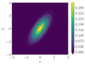
Refer to caption
Refer to caption
(a) Steady-state solution of the Fokker–Planck equation (3.11) with the associated field lines of the probability flux (left) and absolute value of the coefficients of degree less than equal to 101010 in the Hermite expansion (right).
Refer to caption
(b) Convergence of the method, using three different metrics for the error: the L1superscript𝐿1L^{1} norm of the error between the numerical and exact solutions, the negative of the minimum of the numerical solution, and the absolute value of the eigenvalue with smallest real part.
Figure 15: Simulation data when V(x)=x2/2𝑉𝑥superscript𝑥22V(x)=x^{2}/2.

We start with the case V(x)=x2/2𝑉𝑥superscript𝑥22V(x)=x^{2}/2, for which the exact solution to the Fokker–Planck equation (3.10) can be calculated explicitly by substitution of a Gaussian ansatz, see [39, Section 3.7]. We study the convergence of the steady-state solution, obtained by calculating the eigenfunction associated with the eigenvalue of lowest magnitude of Π^dεΠ^dsubscript^Π𝑑superscriptsubscript𝜀subscript^Π𝑑\hat{\Pi}_{d}\,\mathcal{L}_{\varepsilon}^{*}\,\hat{\Pi}_{d}, where Π^dsubscript^Π𝑑\hat{\Pi}_{d} is the L2(𝐑2;eU)superscript𝐿2superscript𝐑2superscripte𝑈L^{2}(\mathbf{R}^{2};\operatorname{e}^{U}) projection operator on Sdsubscript𝑆𝑑S_{d}, directly using the method eigs from the SciPy toolbox. The parameters used for this simulation are the following: β=ε=1𝛽𝜀1\beta=\varepsilon=1, σx2=110superscriptsubscript𝜎𝑥2110\sigma_{x}^{2}=\frac{1}{10}, ση2=1superscriptsubscript𝜎𝜂21\sigma_{\eta}^{2}=1, eU(x,η)/2=eVη(η)/2=eη2/4superscripte𝑈𝑥𝜂2superscriptesubscript𝑉𝜂𝜂2superscriptesuperscript𝜂24\operatorname{e}^{-U(x,\eta)/2}=\operatorname{e}^{-V_{\eta}(\eta)/2}=\operatorname{e}^{-\eta^{2}/4}. With these parameters, the steady-state solution to eq. 3.10 is equal to ρ(x,η)=e2x2+2xηη2/πsubscript𝜌𝑥𝜂superscripte2superscript𝑥22𝑥𝜂superscript𝜂2𝜋\rho_{\infty}(x,\eta)=\operatorname{e}^{-2x^{2}+2x\eta-\eta^{2}}/\pi, and clearly ρL2(𝐑2;eU)subscript𝜌superscript𝐿2superscript𝐑2superscripte𝑈\rho_{\infty}\in L^{2}(\mathbf{R}^{2};\operatorname{e}^{U}). Figure 15 presents the steady-state solution, obtained using the spectral method with Hermite polynomials up to degree 100 (d=100𝑑100d=100) and a triangular index set, and fig. 15 presents the convergence of the method. Since the solution satisfies ρ(x,η)=ρ(x,η)subscript𝜌𝑥𝜂subscript𝜌𝑥𝜂\rho_{\infty}(x,\eta)=\rho_{\infty}(-x,-\eta), the Hermite coefficients corresponding to even values of i+j𝑖𝑗i+j are zero, where i𝑖i and j𝑗j are the indices in the x𝑥x and η𝜂\eta directions, respectively.

Now we consider that V𝑉V is the bistable potential x4/4x2/2superscript𝑥44superscript𝑥22x^{4}/4-x^{2}/2, which was solved numerically in [23] using generalized Hermite functions and a variation of the matrix continued fraction technique. For this case an explicit analytical solution is not available. The parameters we use are the following: β=1𝛽1\beta=1, ε=12𝜀12\varepsilon=\frac{1}{2}, σx2=120superscriptsubscript𝜎𝑥2120\sigma_{x}^{2}=\frac{1}{20}, ση2=1superscriptsubscript𝜎𝜂21\sigma_{\eta}^{2}=1. Through numerical exploration, we noticed that a good convergence could be obtained by using the multiplier function eU(x,η)/2=eβV(x)/2η2/4superscripte𝑈𝑥𝜂2superscripte𝛽𝑉𝑥2superscript𝜂24\operatorname{e}^{-U(x,\eta)/2}=\operatorname{e}^{-\beta V(x)/2-\eta^{2}/4}, rather than just eη2/4superscriptesuperscript𝜂24\operatorname{e}^{-\eta^{2}/4} in the previous paragraph. We note that this would have been the natural choice if the noise in the x𝑥x direction had been white noise. The solution obtained using a square-shaped index set and d=100𝑑100d=100, as well as the corresponding Hermite coefficients up to degree 10, is illustrated in fig. 16. We observe that the Hermite coefficients corresponding to the degree 0 in the η𝜂\eta direction (i.e. to the basis function eη2/2superscriptesuperscript𝜂22\operatorname{e}^{-\eta^{2}/2}) are significantly larger than the other coefficients, which is consistent with the fact that, as ε0𝜀0\varepsilon\to 0, the steady-state solution approaches eβV(x)eη2/2superscripte𝛽𝑉𝑥superscriptesuperscript𝜂22\operatorname{e}^{-\beta V(x)}\,\operatorname{e}^{-\eta^{2}/2} (up to a constant factor). The associated convergence curves are presented in fig. 16. We observe that the convergence is exponential, which is better than the rate of convergence predicted in theorem 3.1.
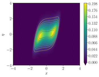
Refer to caption
Refer to caption
(a) Steady-state solution to eq. 3.11 and associated field lines of the probability flux (left), and absolute value of the coefficients of degree less than or equal to 101010 in the Hermite expansion (right).
Refer to caption
Refer to caption
(b) Convergence of the method using the same measures of the error as in fig. 15, except that the L1superscript𝐿1L^{1} error is calculated by comparison with the numerical solution obtained when d=100𝑑100d=100.
Figure 16: Simulation data when V(x)=x4/4x2/2𝑉𝑥superscript𝑥44superscript𝑥22V(x)=x^{4}/4-x^{2}/2.

C.2 McKean–Vlasov equation with colored noise

We focus now on the Galerkin approximation to (3.13). When the potential V()𝑉V(\cdot) is quadratic and the initial condition is Gaussian, it is well-known that the McKean–Vlasov equation has an explicit solution and that this solution is Gaussian. We assume that V(x)=x2/2𝑉𝑥superscript𝑥22V(x)=x^{2}/2 and we rewrite eq. 3.13 in the formalism of [11], as

ρt=(B𝐱ρ+𝐑2K(𝐱𝐱)ρ(𝐱,t)d𝐱ρDρ),𝜌𝑡bold-∇𝐵𝐱𝜌subscriptsuperscript𝐑2𝐾𝐱superscript𝐱𝜌superscript𝐱𝑡differential-dsuperscript𝐱𝜌𝐷bold-∇𝜌\mathchoice{\frac{\partial{\rho}}{\partial t}}{\partial_{t}\rho}{}{}=-\boldsymbol{\mathbf{\nabla}}\cdot\left(B\,\boldsymbol{\mathbf{x}}\,\rho+\int_{\mathbf{R}^{2}}K(\boldsymbol{\mathbf{x}}-\boldsymbol{\mathbf{x}}^{\prime})\,\rho(\boldsymbol{\mathbf{x}}^{\prime},t)\,\mathrm{d}\boldsymbol{\mathbf{x}}^{\prime}\,\rho-D\,\boldsymbol{\mathbf{\nabla}}\rho\right),

where 𝐱=(x,η)T𝐱superscript𝑥𝜂𝑇\boldsymbol{\mathbf{x}}=(x,\eta)^{T} and

B=(1ε1β1/20ε2),K=(θ000),D=(000ε2).formulae-sequence𝐵matrix1superscript𝜀1superscript𝛽120superscript𝜀2formulae-sequence𝐾matrix𝜃000𝐷matrix000superscript𝜀2B=\begin{pmatrix}-1&\varepsilon^{-1}\beta^{-1/2}\\ 0&-\varepsilon^{-2}\end{pmatrix},\quad K=\begin{pmatrix}-\theta&0\\ 0&0\end{pmatrix},\quad D=\begin{pmatrix}0&0\\ 0&\varepsilon^{-2}\end{pmatrix}.

Adapting [11, Proposition 2.3] to our case, we deduce that the solution is of the type

ρ(𝐱,t)=1(2π)|Σ(t)|exp(12(𝐱μ(t))TΣ1(t)(𝐱μ(t))),𝜌𝐱𝑡12𝜋Σ𝑡12superscript𝐱𝜇𝑡𝑇superscriptΣ1𝑡𝐱𝜇𝑡\rho(\boldsymbol{\mathbf{x}},t)=\frac{1}{(2\pi)\,\left|\Sigma(t)\right|}\,\exp\left(-\frac{1}{2}\,(\boldsymbol{\mathbf{x}}-\mu(t))^{T}\Sigma^{-1}(t)(\boldsymbol{\mathbf{x}}-\mu(t))\right),

where μ(t)𝜇𝑡\mu(t) and Σ(t)Σ𝑡\Sigma(t) are given by

μ(t)=eBtμ(0),Σ(t)=et(B+K)Σ(0)et(B+K)T+20tes(B+K)Des(B+K)Tds.formulae-sequence𝜇𝑡superscripte𝐵𝑡𝜇0Σ𝑡superscripte𝑡𝐵𝐾Σ0superscripte𝑡superscript𝐵𝐾𝑇2superscriptsubscript0𝑡superscripte𝑠𝐵𝐾𝐷superscripte𝑠superscript𝐵𝐾𝑇d𝑠\mu(t)=\operatorname{e}^{Bt}\,\mu(0),\quad\Sigma(t)=\operatorname{e}^{t(B+K)}\,\Sigma(0)\,\operatorname{e}^{t{(B+K)}^{T}}+2\,\int_{0}^{t}\operatorname{e}^{s(B+K)}\,D\,\operatorname{e}^{s{(B+K)}^{T}}\,\mathrm{d}s. (C.1)

This solution can be obtained by introducing g=lnρ𝑔𝜌g=-\ln\rho, rewriting eq. 3.13 as an equation for g𝑔g, and using a quadratic ansatz for g𝑔g. The eigenvalue decomposition of B+K𝐵𝐾B+K is

(B+K)(1ε0β(1ε2(1+θ)))=(1ε0β(1ε2(1+θ)))(1θ00ε2),𝐵𝐾matrix1𝜀0𝛽1superscript𝜀21𝜃matrix1𝜀0𝛽1superscript𝜀21𝜃matrix1𝜃00superscript𝜀2(B+K)\begin{pmatrix}1&-\varepsilon\\ 0&\sqrt{\beta}\,(1-\varepsilon^{2}(1+\theta))\end{pmatrix}=\begin{pmatrix}1&-\varepsilon\\ 0&\sqrt{\beta}\,(1-\varepsilon^{2}(1+\theta))\end{pmatrix}\,\begin{pmatrix}-1-\theta&0\\ 0&-\varepsilon^{-2}\end{pmatrix},

which enables the explicit calculation of the integral in the expression of Σ(t)Σ𝑡\Sigma(t). From eq. C.1 and the structure of B𝐵B and K𝐾K, we notice that, as t𝑡t\to\infty, μ0𝜇0\mu\to 0 and

Σ(t)Σ=20es(B+K)Des(B+K)Tds,Σ𝑡subscriptΣ2superscriptsubscript0superscripte𝑠𝐵𝐾𝐷superscripte𝑠superscript𝐵𝐾𝑇d𝑠\Sigma(t)\to\Sigma_{\infty}=2\int_{0}^{\infty}\operatorname{e}^{s(B+K)}\,D\,\operatorname{e}^{s{(B+K)}^{T}}\,\mathrm{d}s,

which coincides with the solution of the steady state linear Fokker–Planck equation corresponding to the McKean–Vlasov equation when m𝑚m is a parameter equal to 0. For this test case, we use the following parameters: β=θ=1𝛽𝜃1\beta=\theta=1, ε=1/2𝜀12\varepsilon=1/2, σx2=ση2=1/5superscriptsubscript𝜎𝑥2superscriptsubscript𝜎𝜂215\sigma_{x}^{2}=\sigma_{\eta}^{2}=1/5, eU(x,η)/2=eV(x)/2eVη(η)/2superscripte𝑈𝑥𝜂2superscripte𝑉𝑥2superscriptesubscript𝑉𝜂𝜂2\operatorname{e}^{-U(x,\eta)/2}=\operatorname{e}^{-V(x)/2}\,\operatorname{e}^{-V_{\eta}(\eta)/2}. The initial condition is taken to be the Gaussian density 𝒩((1,1)T,I2×2)𝒩superscript11𝑇subscript𝐼22\mathcal{N}\left((1,1)^{T},I_{2\times 2}\right). The evolution of the probability density is illustrated in fig. 17, and the convergence of the method, in the L(0,T;L1(𝐑2))superscript𝐿0𝑇superscript𝐿1superscript𝐑2L^{\infty}(0,T;L^{1}(\mathbf{R}^{2})) norm, is illustrated in fig. 18.

Refer to caption
Refer to caption
Refer to caption
Refer to caption
Figure 17: Probability density solution of eq. 3.13 (obtained using the spectral method) at times 0,0.2,0.5,100.20.510,0.2,0.5,1.
Refer to caption
Figure 18: Convergence of the Hermite spectral method for the nonlinear McKean–Vlasov equation with colored noise. The error decreases exponentially for low enough values of d𝑑d, and then reaches a plateau when it becomes dominated by the error induced by the time discretization.

Acknowledgments

The authors are grateful to J.A. Carrillo for making available the finite volume code employed in Subsection 3.1 for the comparison with our spectral method for the McKean–Vlasov dynamics. This work was supported by EPSRC through grants number EP/P031587/1, EP/L024926/1, EP/L020564/1 and EP/K034154/1. The work of SG is supported by the Leverhulme Trust through Early Career Fellowship ECF-2018-536.

References

  • [1] A. Abdulle, G. A. Pavliotis, and U. Vaes. Spectral methods for multiscale stochastic differential equations. SIAM/ASA J. Uncertain. Quantif., 5(1):720–761, 2017.
  • [2] S. Agmon. Lectures on exponential decay of solutions of second-order elliptic equations: bounds on eigenfunctions of N𝑁N-body Schrödinger operators, volume 29 of Mathematical Notes. Princeton University Press, Princeton, NJ; University of Tokyo Press, Tokyo, 1982.
  • [3] E. L. Allgower and K. Georg. Introduction to numerical continuation methods, volume 45 of Classics in Applied Mathematics. Society for Industrial and Applied Mathematics (SIAM), Philadelphia, PA, 2003.
  • [4] N. Bain and D. Bartolo. Critical mingling and universal correlations in model binary active liquids. Nat. Commun., 8:15969, 2017.
  • [5] J. Binney and S. Tremaine. Galactic dynamics, volume 20. Princeton University Press, 2011.
  • [6] G. Blankenship and G. C. Papanicolaou. Stability and control of stochastic systems with wide-band noise disturbances. I. SIAM J. Appl. Math., 34(3):437–476, 1978.
  • [7] V. Bonnaillie-Noël, J. A. Carrillo, T. Goudon, and G. A. Pavliotis. Efficient numerical calculation of drift and diffusion coefficients in the diffusion approximation of kinetic equations. IMA J. Numer. Anal., 36(4):1536–1569, 2016.
  • [8] J. A. Carrillo, A. Chertock, and Y. Huang. A finite-volume method for nonlinear nonlocal equations with a gradient flow structure. Commun. Comput. Phys., 17(1):233–258, 2015.
  • [9] D. A. Dawson. Critical dynamics and fluctuations for a mean-field model of cooperative behavior. J. Statist. Phys., 31(1):29–85, 1983.
  • [10] A. Dhooge, W. Govaerts, Y. A. Kuznetsov, W. Mestrom, A. M. Riet, and B. Sautois. MATCONT and CL MATCONT: Continuation toolboxes in MATLAB, 2006.
  • [11] M. H. Duong and G. A. Pavliotis. Mean field limits for non-Markovian interacting particles: convergence to equilibrium, GENERIC formalism, asymptotic limits and phase transitions. Commun. Math. Sci., 16(8):2199–2230, 2018.
  • [12] A. Durmus, A. Eberle, A. Guillin, and R. Zimmer. An elementary approach to uniform in time propagation of chaos. ArXiv e-prints, May 2018.
  • [13] F. Farkhooi and W. Stannat. A complete mean-field theory for dynamics of binary recurrent neural networks. ArXiv e-prints, Jan. 2017.
  • [14] J. C. M. Fok, B. Guo, and T. Tang. Combined Hermite spectral-finite difference method for the Fokker-Planck equation. Math. Comp., 71(240):1497–1528, 2002.
  • [15] J. Gagelman and H. Yserentant. A spectral method for Schrödinger equations with smooth confinement potentials. Numer. Math., 122(2):383–398, 2012.
  • [16] J. Garnier, G. Papanicolaou, and T.-W. Yang. Large deviations for a mean field model of systemic risk. SIAM J. Financial Math., 4(1):151–184, 2013.
  • [17] J. Garnier, G. Papanicolaou, and T.-W. Yang. Consensus convergence with stochastic effects. Vietnam J. Math., 45(1-2):51–75, 2017.
  • [18] B. D. Goddard, A. Nold, N. Savva, G. A. Pavliotis, and S. Kalliadasis. General dynamical density functional theory for classical fluids. Phys. Rev. Lett., 109:120603, Sep 2012.
  • [19] B. D. Goddard, G. A. Pavliotis, and S. Kalliadasis. The overdamped limit of dynamic density functional theory: rigorous results. Multiscale Model. Simul., 10(2):633–663, 2012.
  • [20] S. N. Gomes, S. Kalliadasis, G. A. Pavliotis, and P. Yatsyshin. Dynamics of the Desai-Zwanzig model in multiwell and random energy landscapes. Phys. Rev. E, 99:032109, Mar 2019.
  • [21] S. N. Gomes and G. A. Pavliotis. Mean field limits for interacting diffusions in a two-scale potential. J. Nonlinear Sci., 28(3):905–941, 2018.
  • [22] S. N. Gomes, G. A. Pavliotis, and U. Vaes. Mean-field limits for interacting diffusions with colored noise: phase transitions and spectral numerical methods. ArXiv e-prints, 2020.
  • [23] P. Hanggi and P. Jung. Colored Noise in Dynamical Systems. Adv. in Chem. Phys., 89:239–326, Jan. 1995.
  • [24] D. J. Higham. An algorithmic introduction to numerical simulation of stochastic differential equations. SIAM Rev., 43(3):525–546, 2001.
  • [25] D. J. Higham, X. Mao, and A. M. Stuart. Strong convergence of Euler-type methods for nonlinear stochastic differential equations. SIAM J. Numer. Anal., 40(3):1041–1063, 2002.
  • [26] W. Horsthemke and R. Lefever. Noise-induced transitions: Theory and application in physics, chemistry, and biology. Springer Series in Synergetics, Springer-Verlag, Berlin, 15, 1984.
  • [27] A. Igarashi, P. V. E. McClintock, and N. G. Stocks. Velocity spectrum for non-Markovian Brownian motion in a periodic potential. J. Statist. Phys., 66(3-4):1059–1070, 1992.
  • [28] A. Igarashi and T. Munakata. Non-Markovian Brownian motion in a periodic potential. J. Phys. Soc. Jpn., 57(7):2439–2447, 1988.
  • [29] E. Jones, T. Oliphant, P. Peterson, et al. SciPy: Open source scientific tools for Python, 2001–2018.
  • [30] B. Krauskopf, H. M. Osinga, and J. Galán-Vioque, editors. Numerical continuation methods for dynamical systems. Understanding Complex Systems. Springer, Dordrecht, 2007.
  • [31] G. Leibon, D. N. Rockmore, W. Park, R. Taintor, and G. S. Chirikjian. A fast Hermite transform. Theoret. Comput. Sci., 409(2):211–228, 2008.
  • [32] L. Lorenzi and M. Bertoldi. Analytical methods for Markov semigroups, volume 283 of Pure and Applied Mathematics (Boca Raton). Chapman & Hall/CRC, Boca Raton, FL, 2007.
  • [33] J. Lu, Y. Lu, and J. Nolen. Scaling limit of the Stein variational gradient descent part I: the mean field regime. ArXiv e-prints, May 2018.
  • [34] E. Luçon and W. Stannat. Transition from Gaussian to non-Gaussian fluctuations for mean-field diffusions in spatial interaction. Ann. Appl. Probab., 26(6):3840–3909, 2016.
  • [35] P. A. Markowich and C. Villani. On the trend to equilibrium for the Fokker-Planck equation: an interplay between physics and functional analysis. volume 19, pages 1–29. 2000. VI Workshop on Partial Differential Equations, Part II (Rio de Janeiro, 1999).
  • [36] P. Monmarché. Long-time behaviour and propagation of chaos for mean field kinetic particles. Stochastic Processes and their Applications, 127(6):1721 – 1737, 2017.
  • [37] S. Motsch and E. Tadmor. Heterophilious dynamics enhances consensus. SIAM Rev., 56(4):577–621, 2014.
  • [38] K. Oelschläger. A martingale approach to the law of large numbers for weakly interacting stochastic processes. Ann. Probab., 12(2):458–479, 1984.
  • [39] G. A. Pavliotis. Stochastic processes and applications, volume 60 of Texts in Applied Mathematics. Springer, New York, 2014. Diffusion processes, the Fokker-Planck and Langevin equations.
  • [40] G. A. Pavliotis and A. M. Stuart. Multiscale methods, volume 53 of Texts in Applied Mathematics. Springer, New York, 2008. Averaging and homogenization.
  • [41] R. Pinnau, C. Totzeck, O. Tse, and S. Martin. A consensus-based model for global optimization and its mean-field limit. Math. Models Methods Appl. Sci., 27(1):183–204, 2017.
  • [42] G. M. Rotskoff and E. Vanden-Eijnden. Neural Networks as Interacting Particle Systems: Asymptotic Convexity of the Loss Landscape and Universal Scaling of the Approximation Error. ArXiv e-prints, May 2018.
  • [43] J. Shen, T. Tang, and L.-L. Wang. Spectral methods, volume 41 of Springer Series in Computational Mathematics. Springer, Heidelberg, 2011. Algorithms, analysis and applications.
  • [44] M. Shiino. Dynamical behavior of stochastic systems of infinitely many coupled nonlinear oscillators exhibiting phase transitions of mean-field type: H theorem on asymptotic approach to equilibrium and critical slowing down of order-parameter fluctuations. Phys. Rev. A, 36:2393–2412, Sep 1987.
  • [45] J. Sirignano and K. Spiliopoulos. Mean Field Analysis of Neural Networks. ArXiv e-prints, May 2018.
  • [46] T. Tang. The Hermite spectral method for Gaussian-type functions. SIAM J. Sci. Comput., 14(3):594–606, 1993.
  • [47] J. Tugaut. Phase transitions of McKean-Vlasov processes in double-wells landscape. Stochastics, 86(2):257–284, 2014.
  • [48] U. Vaes. Python library for the Hermite spectral method. https://github.com/urbainvaes/hermipy, 2018.
  • [49] U. Vaes. Topics in multiscale modelling: numerical analysis and applications. PhD thesis, Department of Mathematics, Imperial College London, 2019.