Searching for Dark Photons with Maverick Top Partners
Jeong Han Kim, Samuel D. Lane, Hye-Sung Lee, Ian M. Lewis, Matthew Sullivan
aDepartment of Physics and Astronomy, University of Kansas, Lawrence, KS 66045, USA
bDepartment of Physics, KAIST, Daejeon 34141, Korea
Abstract
In this paper, we present a model in which an up-type vector-like quark (VLQ) is charged under a new gauge force which kinetically mixes with the SM hypercharge. The gauge boson of the is the dark photon, . Traditional searches for VLQs rely on decays into Standard Model electroweak bosons or Higgs. However, since no evidence for VLQs has been found at the Large Hadron Collider (LHC), it is imperative to search for other novel signatures of VLQs beyond their traditional decays. As we will show, if the dark photon is much less massive than the Standard Model electroweak sector, , for the large majority of the allowed parameter space the VLQ predominately decays into the dark photon and the dark Higgs that breaks the . That is, this VLQ is a “maverick top partner” with nontraditional decays. One of the appeals of this scenario is that pair production of the VLQ at the LHC occurs through the strong force and the rate is determined by the gauge structure. Hence, the production of the dark photon at the LHC only depends on the strong force and is largely independent of the small kinetic mixing with hypercharge. This scenario provides a robust framework to search for a light dark sector via searches for heavy colored particles at the LHC.
1 Introduction
Some of the most important searches for Beyond the Standard Model (BSM) physics at the Large Hadron Collider (LHC) are searches for new vector like quarks (VLQs). Up-type VLQs, so-called top partners , are ubiquitous in composite [1, 2, 3, 4, 5, 6, 7] and Little Higgs [8, 9, 10, 11, 12, 13, 14, 15] models where the top partners help solve the hierarchy problem. Traditionally, searches for VLQs rely on decays into the Standard Model (SM) electroweak (EW) bosons: //Higgs. However, there is a class of “maverick top partners” with non-traditional decays into photons [16, 17, 18, 19, 20, 21], gluons [16, 17, 18, 19, 20, 21], new scalars [22, 23, 24, 25, 26, 27, 28, 29], etc. These new decays can easily be dominant with minor tweaks to the simplest VLQ models. We consider a VLQ that is charged under both the SM and a new abelian gauge symmetry , where the SM is neutral under the . As we will show, in a very large range of the parameter space, this opens new dominant decays of VLQs that have not yet been searched for.
This new can be motivated by noting that dark matter may very well have self-interactions through this new force. The gauge boson, the so-called dark photon, kinetically mixes with the SM hypercharge through a renormalizable interaction [30, 31, 32]. This kinetic mixing can be generated via new vector like fermions charged under both the SM and the new [30, 33, 34], as considered here. In the limit that the dark photon is much less massive than the Z and the kinetic mixing is small, the dark photon inherits couplings to SM particles of the form , where is the electromagnetic current and is the kinetic mixing parameter. Hence, the name dark photon. Most of the searches for the dark photon take place at low energy experiments such as fixed target experiments or B-factories [32]. However, it is also possible to search for dark photons through the production and decays of heavy particles at high energy colliders [35, 36, 37]. For example, Higgs decays [33, 38, 34] into dark photons is a plausible scenario for discovery.
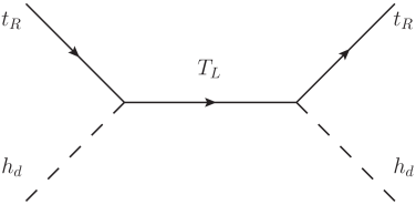
A recent paper [39] studied the scenario where down-type VLQs and vector like leptons are charged under the SM and . Ref. [39] relied on a very large mass gap between the SM fermions and their vector-like fermion partners to suppress the traditional vector-like fermion decays into //Higgs. With this mass gap, the branching ratios of vector-like fermions into dark photons and SM fermions is enhanced. Here we point out that this mechanism does not require a mass gap in the fermion sector, although such a gap further enhances the effect. To illustrate this, we will focus on an up-type VLQ, , that mixes with the SM top quark, . The mass gap between and does not need to be as large as between the bottom quark/leptons and vector-like fermions. From the Goldstone equivalence theorem, the partial width of into fully SM final states is
where is a mixing angle between the SM top quark and , GeV is the Higgs boson vacuum expectation value (vev), and is the mass of the VLQ . The partial width is inversely proportional to due to an enhancement of decays into longitudinal s and s. If the new vector like quark is charged under the dark force (and assuming there is a dark sector Higgs mechanism), the partial widths of into the dark photon, , or dark Higgs, , is
where is the vev of the dark sector Higgs boson. Note that now the partial width is inversely proportional to . Hence, the ratio of the rates into and is
For dark photon masses GeV, we generically expect that the vev GeV and
Hence, the VLQ preferentially decays to light dark sector bosons due to the mass gap between the dark sector bosons and the SM EW bosons. Since there is a quadratic dependence on and , this mass gap does not have to be very large for the decays to be dominant.
This is a new avenue to search for light dark sectors using decays of heavy particles at the LHC, providing a connection between heavy particle searches and searches for new light sectors. The appeal of such searches is that pair production of VLQs is through the QCD interaction and is fully determined via gauge interactions. That is, the pair production rate only depends on the mass, spin, and color representation of the produced particles. Additionally, as we will show, for a very large region of parameter space VLQs will predominantly decay into dark photons and dark Higgses. Hence, the dark photon can be produced at QCD rates at the LHC independently of a small kinetic mixing parameter. The major dependence on the kinetic mixing parameter arises in the decay length of the dark photon, and for small the dark photon can be quite long lived. In fact, for small dark photon masses, its decay products will be highly collimated and may give rise to displaced “lepton jets” [40].
In Section 2 we present an explicit model that realizes this mechanism for dark photon searches and review current constraints in Sec. 3. We calculate the decay and production rates of the new VLQ in Sec. 4 and the decay of the dark photon in Sec. 5. In Section 6 we present collider searches relevant for our model. This includes the current collider sensitivity as well as demonstrating the complementarity between the searches for dark photons via heavy particle decays at the LHC and low energy experiments. Finally we conclude in Section 7. We also include several appendices with the details on perturbative unitarity calculation in App. A, kinetic mixing in App. B, relevant scalar interactions in App. C, and relevant dark photon-fermion couplings in App. D.
2 Model
We consider a simple extension of the SM consisting of a new singlet up-type vector-like quark, , and a new gauge symmetry. For simplicity, we will only consider mixing between the new vector-like quark and generation SM quarks:
| (1) |
The SM particles are singlets under the new symmetry, and we give the VLQ a charge under the new symmetry. The is broken by a dark Higgs field that is a singlet under the SM and has charge under . The relevant field content and their charges under are given in Table 1. This particle content and charges are similar to those in Ref. [39].
This field content allows for kinetic mixing between the SM field, , and the new gauge boson, :
where are the field strength tensor with and are the field strength tensors with The relevant fermion kinetic terms for the third generation quarks and VLQ are
| (3) |
and the relevant scalar kinetic terms are
| (4) |
The general covariant derivative is
| (5) |
where is the strong coupling constant, is the coupling constant, is the coupling constant, and is the coupling constant. Values for , and the generators of , are given according to the charges in Table 1.
| 3 | 1 | 2/3 | 0 | |
| 3 | 1 | -1/3 | 0 | |
| 3 | 2 | 1/6 | 0 | |
| 1 | 2 | 1/2 | 0 | |
| 3 | 1 | 2/3 | 1 | |
| 3 | 1 | 2/3 | 1 | |
| 1 | 1 | 0 | 1 |
2.1 Scalar Sector
The allowed form of the scalar potential symmetric under the gauge group is
| (6) |
Since does not break EW symmetry, must have a vev of GeV. Imposing that the potential has a minimum where the SM Higgs and dark Higgs have vacuum expectation values and , the mass parameters are found to be
| (7) |
Now we work in the unitary gauge:
| (8) |
The two Higgs bosons mix and can be rotated to the mass basis:
| (9) |
where can be identified as the observed Higgs boson with a mass GeV, and is a new scalar boson with mass . After diagonalizing the mass matrix, the free parameters of the scalar sector are
| (10) |
All parameters in the Lagrangian can then be determined
| (11) |
where .
To check the stability of the scalar potential, we consider it when the fields and are large:
| (12) | |||||
where in the last step we completed the square. The potential is bounded when
| (13) |
From the relationships in Eq. (11) we have
| (14) |
Hence, the boundedness condition for the potential is always satisfied as long as and are both positive.
For our analysis in the next sections, only two trilinear scalar couplings are relevant:
| (15) |
where
| (16) | |||||
2.2 Gauge Sector
From Eq.(2), the gauge boson can mix with the SM electroweak gauge bosons. After diagonalizing the gauge bosons, the covariant derivative in Eq. (5) becomes
where is a mixing angle between the dark photon and SM -boson; and are the usual electromagnetic charge and operator respectively; and with are the neutral current coupling and operator respectively; ; is the observed EW neutral current boson with mass ; and is the dark photon with mass . Additionally, is the mixing angle between and . The relationship between and other model parameters is not the same as the SM weak mixing angle. Hence, we introduce the hat notation to emphasize the difference. The relationship between the SM weak mixing angle and is given below111The details of diagonalizing the gauge boson kinetic and mass terms, including precise definitions of and , are given in Appendix B.. For simplicity of notation, we have redefined the coupling constant and kinetic mixing parameter
| (18) |
The SM EW sector has three independent parameters, which we choose to be the experimentally measured mass, the fine-structure constant at zero momentum, and G-Fermi [41]:
| (19) |
In addition to the EW parameters, we have the new free parameters:
| (20) |
All other parameters in the gauge sector can be expressed in terms of these. Since , we can solve equations for and iteratively as an expansion in :
where and the SM value of the weak mixing angle is
| (21) |
Although these are good approximations for , unless otherwise noted we will use exact expressions of parameters as given in Appendix B.
Note that in the limit of small kinetic mixing and dark photon mass much less than the -mass we find the covariant derivative
where the superscript indicates the SM value of parameters. Hence we see that the dark photon couples to SM particles through the electromagnetic current with coupling strength . Additionally, the -boson obtains additional couplings to particles with non-zero dark charge with strength .
2.3 Fermion Sector
To avoid flavor constraints, we only allow the VLQ to mix with the third generation SM quarks. The allowed Yukawa interactions and mass terms that are symmetric under are
| (23) |
After symmetry breaking, the VLQ and top quark mass terms are then
| (24) |
where
| (25) |
and . To diagonalize the mass matrix, we perform the bi-unitary transformation:
| (26) |
where and are the mass eigenstates with masses GeV and , respectively. Since the Lagrangian only has three free parameters, the top sector only has three inputs which we choose to be
| (27) |
The Lagrangian parameters can be expressed by
| (28) | |||||
| (29) | |||||
| (30) |
The right-handed mixing angle is redundant and can be determined via
| (31) |
After rotating to the scalar and fermion mass eigenbases, the couplings to the third generation and VLQ are given by
where the couplings are
| (33) | |||||
and the couplings are
| (34) | |||||
Now we consider the small angle limit . If the VLQ and top quark have similar masses , then Eq. (30) becomes . In this limit, from Eq. (31), we see that and both mixing angles are small. However, for a large fermion mass hierarchy , the right-handed mixing angle expressions in Eq. (31) become
| (35) |
There are two cases then:
| (36) |
where the sign of depends on the sign of . Hence, as discussed in Ref. [39], the right-handed mixing angle is enhanced relative to the left-handed mixing angle due to a large fermion mass hierarchy.
Since and have different quantum numbers and mix, flavor off-diagonal couplings between the VLQ and the SM third generation quarks appear. In the small mixing angle limit, the relevant couplings are
| (40) |
The full Feynman rules are given in Appendix D. Note that although the right-handed coupling to the appears of order , if the left- and right-handed couplings can be of the same order. However, with this counting the right-handed coupling of the dark photon, VLQ, and top quark is unsuppressed. This is precisely the fermionic mass hierarchy enhancement noticed in Ref. [39]. However, as we will point out, a fermionic mass hierarchy is not necessary for the VLQ decays into the dark Higgs or dark photon to be dominant.
3 Current Constraints
3.1 Electroweak Precision and Direct Searches
Electroweak precision measurements place strong constraints on the addition of new particles. In the model presented here, there are many contributions to the oblique parameters [42, 43, 44]: new loop contributions from the VLQ [45, 46, 47, 48, 49, 50] and scalar [51, 52, 53, 54, 55, 56] as well as shifts in couplings to EW gauge boson couplings from the mixing of the dark photon with hypercharge [57, 35], dark Higgs with the SM Higgs, and the VLQ with the top quark. Since there are multiple contributions to the oblique parameters in this model, there is the possibility of cancellations that could relax some of the constraints. To be conservative, we will only consider one contribution at a time.
There are also many direct searches for VLQs, new scalars, and dark photons at colliders and fixed target experiments. Here we summarize the current state of constraints:
-
•
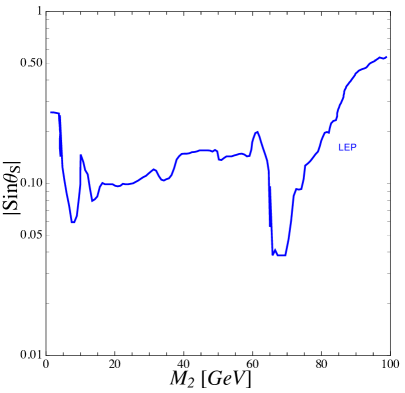
VLQ: The dashed line labeled “EW Prec” in Fig. 1 shows the EW precision constraints on the VLQ-top quark mixing angle. This result is taken from Ref. [50]. The current limits are () for VLQ mass TeV (2 TeV).
Additionally, in our model the top-bottom component of the CKM matrix is , where the subscript SM denotes the SM value. The most stringent constraints on come from single top quark production. A combination of Tevatron and LHC single top measurements give a constraint of [41]. Another more recent analysis including differential distributions gives a bound of [58]. Both constraints give an upper bound of at the confidence level. This limit is indicated by the orange dotted line labeled “CKM” in Fig. 1, where the region above is excluded. We see that the CKM measurements are not currently as important as EW precision constraints.
As mentioned above, in the model presented here traditional decays into SM EW bosons Higgs will be suppressed and not directly applicable. Nevertheless, for completeness we summarize their results here. In these traditional modes, the LHC excludes VLQ masses TeV in pair production searches [59, 60, 61] and TeV in single production searches [62, 63, 64]. Single production of an singlet depends on the mixing angle and decouples as [16] weakening the above limit. Taking this into account, LHC searches for single production have been cast into constraints on which are comparable to EW precision constraints for TeV [65, 62].
-
•
Scalar: The addition of a new scalar shifts Higgs boson couplings away from SM predictions, as well as contributing to new loop contributions to EW precision parameters. Additionally, many searches have been performed for new scalar production at the LHC [66, 67, 68, 69, 70, 71, 72] as well as at LEP [73, 74, 75]. However, the most stringent constraints [76] come from precision measurements of the observed GeV Higgs boson for GeV and precision -mass constraints [55, 56, 77] for TeV. The constraints on the scalar mixing angle is for TeV [76]. For GeV LEP searches can be very constraining on the scalar mixing angle, as shown in Fig. 1. These results are adapted from Ref. [56].
-
•
Kinetic Mixing: As can be seen in covariant derivative in Eq. (2.2), the couplings between the and SM particles are shifted due to the kinetic mixing of the Hypercharge and gauge boson. Hence, electroweak precision data can place bounds on the value of the kinetic mixing parameter [57, 35]. The most stringent constraints from EW precision are [35]. This is less constraining than direct searches for dark photons at fixed target experiments or low energy experiments [78] which require for GeV.

3.2 Perturbativity Bounds
Requiring the top quark and VLQ Yukawa couplings be perturbative can place strong constraints on the top quark-VLQ mixing angle. As can be seen in Eq. (29), in the limit that the Yukawa couplings become
| (41) |
While is well-behaved for , is enhanced by . Hence, the mixing angle must be small to compensate for this and ensure remains perturbative.
To determine when becomes non-perturbative, we calculate the perturbative unitarity limit for the scattering process and find that
| (42) |
When this limit is saturated, there must be a minimum higher order correction of to unitarize the S-matrix [79]. Hence, this is near or at the limit for which we can trust perturbative calculations. Details of this calculation can be found in Appendix A.
To translate the limit on to a limit on the mixing angle we solve Eq. (29) to find
| (43) |
This solution is real if . Combining with the perturbative unitarity limit in Eq. (42), we find an upper limit on :
| (44) |
Note that for VLQ mass , the perturbative unitarity limit is never saturated. Hence, for a fixed there is an upper bound on for which is always perturbative. Assuming , the upper-bound on becomes
| (45) |
In Fig. 1 we show the limits on from (solid) requiring that satisfies Eq. (44) for various values of together with (dashed magenta) EW precision data and (dotted orange) CKM constraints. The kink in the GeV line occurs at VLQ mass GeV. For the upper bound on is proportional to , while for it is proportional to as shown in Eq. (45). As can be clearly seen, over much of the parameter range the limits on in Eq. (44) provide the most stringent constraint on . As mentioned earlier, this is due to having an enhancement of , requiring to be quite small to ensure does not get too large. EW precision is more constraining for larger and smaller .
3.3 Limits
There have been searches at the LHC [80] for where that place limits on combination
| (46) |
for dark photons in the mass range . The subscript indicates a SM production rate. The production rate is dominantly via gluon fusion which in the model presented here is altered via the shift in the coupling away from the SM prediction as shown in Eqs. (2.3,33) and new loop contributions from the new VLQ. However, in the small mixing angle limit with the counting , we have
| (47) |
In addition to the usual SM decay modes, can decay into , , and when kinematically allowed. Using the counting , the partial widths into the new decay modes are
| (48) | |||||
For the decays into SM, all the couplings between and SM fermions and gauge bosons, except for the and couplings, are uniformly suppressed by . The and couplings are more complicated due to the mixing and mixing, respectively. Additionally, there are new contributions to the loop level decays , , and due to the new VLQ. Since the partial widths and make negligible contributions to the total width, we will neglect changes in these quantities. Reweighting the SM partial widths with the new contributions, the width into fully SM final states are then
| (49) | |||||
| (50) |
where are SM fermions or gauge bosons, the subscript indicates SM values of widths, MeV [81], and , are in Eq. (33). Other SM values for the partial widths of can be found in Ref. [81]. The loop function can be found in Ref. [82], where and we have used such that .

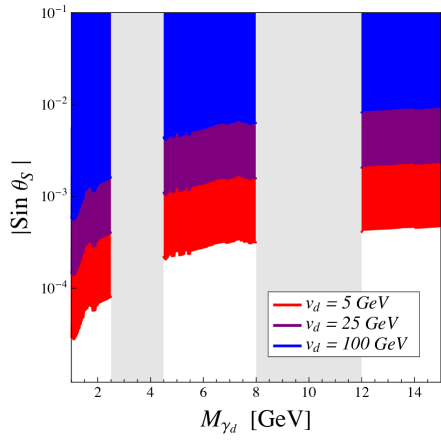
ATLAS has measured the upper limit in the mass range GeV when both dark photons decay into muons [80]. However, they have assumed neglecting possible hadronic decays of the dark photon. We reweight the results of Ref. [80] using the including hadronic decays222See Sec. 5 for details of the calculation., as shown in Fig. 2. The hatched regions correspond to hadronic resonances and were not included in the search in Ref. [80]. This is the to be used in Eqs. (46,53).
In Fig. 2 we show the upper limit on from Eq. (53) and using in Fig. 2. The solid regions are ruled out by the search for (red) GeV, (maroon) GeV, and (blue) GeV. These constraints are very strong with limits in the range of . These limits are more constraining than the direct searches for as shown in Fig. 1. Eq. (53) is linear in the dark Higgs vev , so the limits on become less constraining for large . However, since these constraints cannot be arbitrarily relaxed without very small dark gauge coupling .
If there is dark matter (DM) with mass , it is possible that the decay of the dark photon into DM is dominant since, unlike the dark photon coupling to SM fermions, the -DM coupling would not be suppressed by the kinetic mixing parameter . Hence, it is possible for the Higgs to decay invisibly . There are searches for invisible decays of with limits [83] from CMS and from ATLAS [84]. Assuming that , from Eq. (53) these limits correspond to
| (54) |
4 Production and Decay of Vector Like Quark
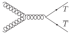

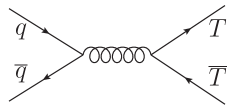

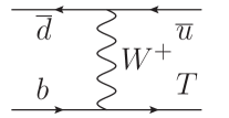
In this section, we focus on the production and decay of the VLQ, , at the LHC based on the model in Sec. 2. Figure 3 displays the VLQ (a,b,c) pair production () and (d,e) single production in association with a jet ( + jet)333There is also production which is subdominant. In the model with an additional singlet scalar, a loop-induced production [16] can be as large as the pair production.. The pair production is induced by QCD interactions so that the production cross section depends only on , the spin of , and the gauge coupling. Hence, pair production is relatively model independent444In a scenario where the top partners are pair produced via a heavier resonance, the production cross section can be model dependent. See Refs. [86, 87, 88] and references therein.. The single production, on the other hand, relies on the coupling in Eq.(40) which is proportional to the mixing angle . Therefore the production cross section is proportional to and is suppressed for small [16].
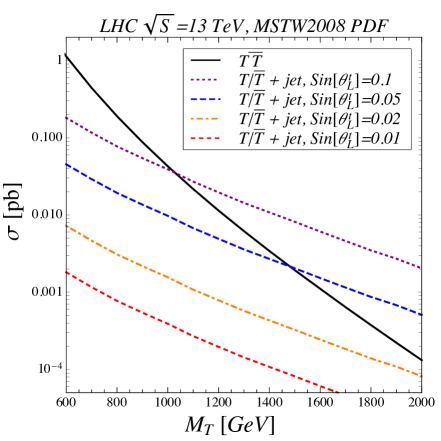
In Fig. 4 we show cross sections for single and pair production of from Ref. [85]555It should be noted that these results are for a charge 5/3 VLQ. However, a charge 2/3 partner has the same QCD and spin structure so the results are still valid since the QCD production does not depend on the electric charge of the particle.. The pair production cross section with NNLO QCD corrections is computed using the HATHOR code [89] with the MSTW2008 parton distribution functions (PDF) [90]. The single production cross section with NLO QCD corrections is calculated using MCFM [91, 92, 93] with the same PDF. The NLO single production cross sections are rescaled by to take into account the normalization of the coupling in Eqs.(40,101). The single production becomes more important at high mass, where the gluon PDF sharply drops suppressing and the pair production phase space is squeezed relative to single production. With a sizable mixing angle , the single production outperforms the pair production in a wide range of . The single production, however, vanishes as the mixing angle becomes very small, as required by perturbativity and EW precision [Fig. 1]. This can be already seen from Figure 4 when , where the jet cross section goes into the sub-femtobarn level which will be challenging to probe at the LHC.


Traditionally, searches for the VLQ rely on the , , and decays, as shown in Fig 5. However, in the scenario where is charged under both the SM and , new decay modes into the and appear, which alters phenomenology significantly. Partial widths into in the limit and are666To produce numerical results and plots, however, we will use exact width expressions.


| (55) |
For large , the partial widths of into fully SM final states are proportional to due to the Goldstone equivalence theorem. The partial widths into and in the limit and are
| (56) |
Hence, the ratios of the rates of VLQ decays into the dark Higgs/photon and into fully SM final states are
| (57) |
There are two enhancements: (1) the enhancement since decays into longitudinal dark photons are enhanced by compared to decays into longitudinal SM bosons which are proportional to . (2) If there is a enhancement since the right-handed top-VLQ mixing angle is larger than left-handed mixing due to a fermion mass hierarchy as seen in Eqs. (35-40). However, note that for fixed , the fermion mass hierarchy enhancement cancels and only the survives. Although, note there is now a suppression from the fermion mass hierarchy and is disfavored by perturbative unitarity [Eq. (45)]. This is because in this limit and does not grow with .
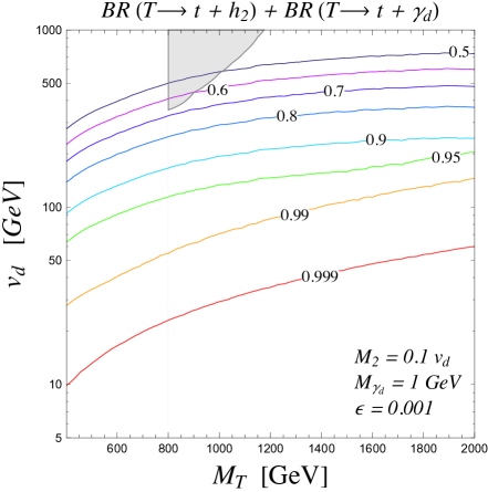
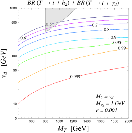
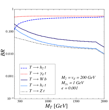
Equation (57) shows that even in the absence of a fermionic mass hierarchy (), decays into light dark sector bosons are still strongly enhanced. This can be clearly seen in Figure 6(a,b) where we show contours of the total VLQ branching ratio in and . Note that for GeV in the entire range. As increases, branching ratios into the dark photon/Higgs increase due to the fermionic mass hierarchy, as discussed above. Fig. 6 is the same as Fig. 6 with a different choice of . The results in both Fig. 6(a,b) are very similar, showing the conclusions about the branching ratio dependence on boson and fermion mass hierarchies are robust against model parameters. The reach of current searches into and [59] are shown in the gray shaded regions. We have rescaled the results of Ref. [59] according to the branching ratios in our model. There were no limits below GeV, hence the exlusion region is truncated. As can be seen, the traditional searches are largely insensitive to our model and our approach provides a new avenue to search for . New search strategies are necessary depending on the decays of as we will discuss in section 6.
In Fig. 6(c,d) we show the branching ratios of into all final states, including . The branching ratios into the fully SM particles are less than for smaller GeV as shown in Fig. 6. For enhanced dark sector mass scales GeV the rates to the SM final states can reach at most for GeV shown in Fig. 6, but then fall to the percent level for higher VLQ masses.
There is a kink in Fig. 6 around TeV. For TeV EW precision constraints on are the most stringent and for TeV the perturbativity bounds on are most constraining [see Fig. 1]. The EW precision and perturbativity bounds on have different dependendencies on , hence the kink. The branching ratios into Higgs become flat for approaching 1.9 TeV. Without perturbative unitarity constraints, these branching ratios would eventually increase due to the suppression of by the fermionic mass hierarchy for the limit of and fixed , as discussed around Eq. (57). Perturbative unitarity instead prevents this increase from occurring. Once perturbativity constraints are dominant , the fermion mass hierarchy enhancement reasserts itself, and branching ratios into fully SM final states decrease precipitously.
Finally, in the limit and , the total width of the VLQ normalized to is
| (58) |
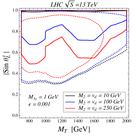
Due to the very large enhancement of , the mixing angle must be quite small for to be narrow. In Fig. 7 we show contours of fixed in the plane for various dark Higgs vevs . When compared to the constraints in Fig. 1, it is clear that the constraint be narrow with is by far the strongest constraint on . In Fig. 7 we show the total width in the plane. As is clear, VLQ total width grows for small and larger .
5 Decay of the dark photon
We now discuss the dark photon decays, since this specifies experimental signatures in the VLQ decay . The lowest order (LO) partial decay widths can be computed using the couplings to the light fermions from the covariant derivative in Eq. (2.2). However, this does not take into account the higher-order QCD corrections and hadronic resonances. To reflect these combined effects, we follow Ref. [35] and utilize the experimental data on electron positron collisions [41]
| (59) |
Since couplings are approximately electromagnetic, hadronic decays of can be incorporated into the total width of via
| (60) | |||||
We have used the approximation and as in Eq. (2.2). We have also assumed there are no DM candidates with mass and that so that DM and decays are forbidden.

The lifetime of the dark photon can be calculated by
| (61) |
Hence, the lifetime is inversely proportional to . For small kinetic mixing parameter the dark photon can be quite long lived and have a large decay length. In Fig. 8 we show the decay length of the dark photon as a function of the kinetic mixing parameter for various dark photon masses. For in the range of the decay length can be mm. As discussed in the next section, this can lead to a spectacular collider signature of displaced vertices.
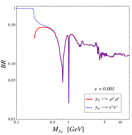
In Fig. 8 we show the branching ratios of the dark photon into electrons and muons. This reproduces the results from Ref. [35], which we have recalculated and included for completeness. The branching ratios of the dark photon into electrons and muons are almost identical when . For much lower masses below MeV, the decay to muons is kinematically closed, and hence decays dominate. The multiple dips in the branching ratios starting around MeV are attributed to hadronic resonances , , , , , , and for [41].
6 Searching for the dark photon with decays
We now discuss the collider signatures of this model. As discussed previously, the pair production of only depends on the spin and mass of and in a very large range of parameter space. Hence, the production rate of the dark photon is at QCD rates and largely independent of the model parameters. The major model dependence comes from the lifetime of . If is sufficiently small, the dark photon becomes long-lived.
The decay length of the dark photon from decays is
| (62) |
where is a proper lifetime as shown in Fig. 8 and is the average boost of the dark photon. Assuming the VLQs are produced mostly at rest, the boost is
where is the dark photon 3-momentum. Using the total width in Eq. (60), we can then solve for the decay length:
| (64) |
Hence, for reasonable parameter choices, the decay length of the dark photon can be several hundreds of microns. The precise direction of the dark photon in the detector will determine if it appears as a displaced vertex or where it will decay in the detector. Nevertheless, for m the dark photon decay can be considered prompt, for it will be a displaced vertex, for the dark photon will decay in the detector, and the dark photon will decay outside the detector [16]. Hence, we can solve for the values of for these various scenarios:
If the dark photon decays outside the detector it is unobserved, giving rise to the final state characterized by . This is the same signature as pair produced scalar tops, , in R-Parity conserving SUSY models with the decays , where is the lightest superpartner and stable. Hence, the currently available CMS [94, 95, 96, 97, 98, 99] and ATLAS [100, 101] searches for stop pair production can be used to obtain constraints on the model presented here. In the limit of large gluino/squark masses, the most stringent bound is at 13 TeV excludes stop masses up to 1225 GeV for a massless [99]. Since Ref. [99] assumes , the corresponding CL upper limit on the NLL-NLO stop pair production cross section is given by fb [102].
Since both stop and pair production yield similar kinematic distributions in the final states, the efficiencies of two searches are quite similar [103]. The upper bound on the stop pair production cross section can then be reinterpreted as a bound on the VLQ pair production cross section:
| (66) |
In Fig. 9 we show this limit in the plane for a dark photon mass of GeV (gray region is ruled out). We used the branching ratios in Fig. 6 and the NNLO cross section in Fig. 4. As shown in Sec. 4, the production and decay rates of the VLQ are relatively independent of model parameters and this result is robust. We find that VLQ masses
| (67) |
are excluded for GeV and GeV when the dark photon is stable on collider time scales. The bound can be weakened for higher values of since the branching ratio of into SM bosons with visible decays increases, suppressing as displayed in Figure 6.


Searches for single production can be important if mixing is not too small. It is clear from Figure 4 that for the single production dominates over the pair production at high VLQ masses. Refs. [125, 126] showed that the channel displays a superior performance in prospects for discovering the . The signature is then , which is the same as for when is long lived. The ATLAS collaboration [104] presented results on the single production of with the decay . Assuming that efficiencies of and searches are the same, we re-interpret the CL upper limit on the cross section in Ref. [104] to derive constraints on plane, as shown as dotted lines in Figure 9. The regions within the curves are ruled out. As in Fig. 9, we consider both where the dark photon is assumed to escape the detector, and . For VLQ masses around TeV, the limits on are
| (68) |
where the stronger bounds are expected for smaller values of due to the enhancement of the branching ratio . For smaller the single VLQ production rate is too small to be detectable yet. For larger and larger , the VLQ essentially decays like a top quark with a near 100% branching ratio into . Hence, the branching ratio to is suppressed and a gap appears for and GeV. These bounds are, however, weaker as compared to the EW precision test [see Figure 1].
CMS has also performed a recent search for electroweak production of T decaying through Z and Higgs channels with fully hadronic decays [105]. These searches can be re-interpretted into constraints in the plane. The % CL exclusions are shown as solid lines in Figure 9 with the regions inside the curves ruled out. In the small limit ( GeV) the branching ratios into SM final states are neglible so there are not strong constraints. As increases the branching ratios become viable and some constraints emerge. In the high the generic search constraints start to become more stringent than constraints. Hence, there is a complementarity between the fully hadronic and missing energy searches.
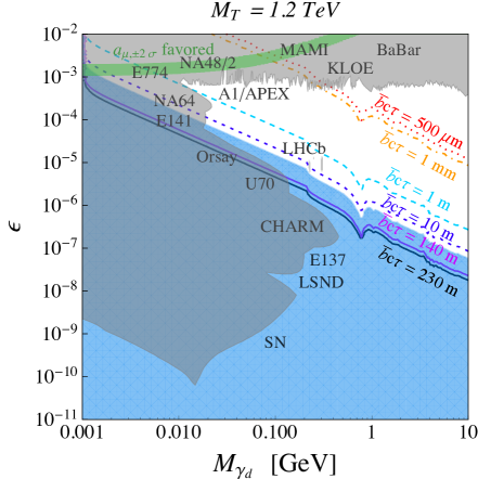
Figure 10 shows the decay lengths of dark photons originating from the VLQ with masses (a) TeV and (b) TeV in plane. We show several lines of the dark photon decay length that are indicative of prompt decays (=500 m), displaced vertices (=1 mm), decays in the detector (=1 m), and decays outside the detector (=10 m). Additionally, there is a proposed MATHUSLA detector [127] to search for long lived particles. MATHUSLA will be on the surface m away from the interaction point. Hence, we also show lines for dark photons that could decay inside the MATHUSLA detector. The blue shaded regions are excluded by searches for stop pair production with decay , as discussed above. This blue exclusion region exists for TeV. Hence, it appears in Fig. 10 but not Fig. 10. The grey shaded regions are excluded by various low energy experiments [78] and supernova measurements [123, 124]. As can be clearly seen, searches for with a wide range of possible signals can cover a substantial portion of the parameter space. This is because in the model presented here the production of from VLQ production is largely independent of the small kinetic mixing parameter. Hence, the production rate of is unsuppressed at low and the LHC can be quite sensitive to this region.
The dark photon branching ratios into and is non-negligible as shown in Fig. 8. Hence, the most promising signature of the would be the leptonic decays of the dark photon, which would help avoid large QCD backgrounds. Since the dark photon is highly boosted, its decay products are highly collimated. The angular distance between the leptons from decays can be estimated as
| (69) |
where , are the azimuthal angles of the leptons, and are their rapidities. At such small angular separation, the leptons are very difficult to isolate and the dark photon can give rise to so-called “lepton jets” [40, 39] which are highly collimated clusters of electrons and muons. In fact, for not too small kinetic mixing , there could be displaced lepton jets or even lepton jets originating in the detector.
7 Conclusion
In this paper we have studied a model with an up-type VLQ charged under a new , where the gauge boson kinetically mixes with the SM hypercharge. One of the most significant aspects of this model is that the decay patterns of the VLQ can be substantially altered from the usual scenario. That is, the VLQ is a “maverick top partner.” As shown in Figs. 6(a,b), if the scale of the is smaller than the EW sector (), the VLQ decays into a dark photon or dark Higgs greater than of the time independent of the VLQ mass. This is due to the longitudinal enhancement of decaying into light gauge bosons which enhances the VLQ partial widths into by relative to decays into the SM EW bosons. When the VLQ is substantially heavier than the top quark , there can also an enhancement of for VLQ decays into [39].
The appeal of this scenario is that the production rate of the dark photon is largely independent of model parameters. The VLQs can be pair produced via the strong interaction. This pair production rate is governed by gauge interactions and only depends on the VLQ mass and spin. As discussed above, the branching ratio in a very wide range of parameter space. Hence, the dark photon production rate is almost completely governed the strong interaction and is independent of the small kinetic mixing parameter .
While the production rate of the dark photon is independent of the kinetic mixing parameter, the collider searches are not. As we showed, for reasonable , the dark photon can give rise to displaced vertices, decay inside the detector, or even escape the detector and appear as missing energy as shown in Fig. 10. Besides the missing energy, the most promising signatures of the dark photon would be its decays into electrons and muons. For dark photon masses much below the VLQ masses, the electrons and muons would be highly collimated giving rise to lepton jets [40] or even displaced lepton jets.
The model presented here is a mild perturbation from the typical simplified models of dark photons and VLQs. However, as we demonstrated, the collider phenomenology is significantly changed from the usual scenarios. Hence, this provides a robust framework in which searches for heavy particles at the LHC can illuminate a light dark sector force.
Acknowledgements
We would like to thank KS Babu, KC Kong, and Chris Rogan for helpful discussions. We would also like to thank KC Kong and Douglas McKay for suggestions the term “maverick top partner.” JHK and IML are supported in part by the U.S. Department of Energy under grant No. DE-SC0017988. MS is supported in part by the State of Kansas EPSCoR grant program. SDL acknowledges financial support of Madison & Lila Self Graduate Fellowship. HSL is supported by National Research Foundation (NRF) Strategic Research Program (NRF2017R1E1A1A01072736). The data to reproduce the plots has been uploaded with the arXiv submission or is available upon request.
Appendix A Perturbative Unitarity
To derive a perturbative unitarity bound, we will look at tree-level scattering in the high energy limit. For the high energy limit, we work with gauge eigenstate fields in the unbroken phase. In the broken phase, there would be -channel diagrams with scalar trilinears. However, since trilinear scales are dimensionful, they will be suppressed by compared to the fermionic -channel, were is the energy of the process.
Additionally, each vertex flips the chirality of the fermion. In the high energy limit, we neglect masses, so there can be no additional chiral flips from mass insertions. Hence, the chirality of the incoming and outgoing top quarks must be the same. Finally, the dark higgs vertex only exists between and , so only the amplitudes are non-zero. Fig. 11 shows the relevant diagram.
The tree-level amplitude for this process is given by
| (70) |
where is the scattering angle. We now expand this amplitude into partial waves as
| (71) |
where are Wigner d-functions. The only relevant term for this particular process corresponds to the term, and we get
| (72) |
Tree-level perturbative unitarity then corresponds to , which, after taking a square root, gives us the final form of our bound,
| (73) |
Appendix B Kinetic Mixing
We now review diagonalizing the neutral gauge bosons. First, the kinetic mixing term in Eq. (2) with the transformations
| (74) |
where . Then we have the normalized gauge kinetic terms
| (75) |
The covariant derivative in Eq.(5) then contains
| (76) |
where we have defined , .
| (77) |
Here, is identified as the SM-like hypercharge gauge boson. To get the photon we perform the usual rotation:
| (78) |
where . The covariant derivative becomes
where , , , and . The charge operator is . Hence, and in the unitary gauge. We can identify as the physical massless photon and as the electric charge.
Evaluate the scalar kinetic terms to get the gauge boson masses:
| (79) | |||||
where
| (80) |
and . We rotate the basis to diagonalize the mass matrix
| (81) |
where has mass and has mass . We can solve for the mixing angle and masses
| (82) | |||||
| (83) | |||||
| (84) |
Now, for the degrees of freedom we choose:
| (85) |
with the values in Eq. (19). Using together with and Eqs. (80,83), we find
| (86) |
where . Now, Eqs. (82,86) can be used to recursively solve for as an expansion in . All other parameters can then be easily solved for in terms of the input parameters in Eq. (85).
Appendix C Scalar Interactions
The scalar couplings relevant the analysis here are
| (87) |
The detailed expressions for the couplings are
| (88) | |||||
| (89) | |||||
| (90) | |||||
| (91) | |||||
| (92) | |||||
| (93) | |||||
| (94) | |||||
| (95) |
where are given in Eq.(80). The detailed expressions for gauge-sector parameters can be found in Appendix B.
The trilinear are given by
| (96) |
where the couplings are
| (97) | |||||
| (98) | |||||
| (99) | |||||
| (100) |
Appendix D Gauge Boson Fermion Interactions
The interactions with the top quark and VLQ are
| (101) |
The couplings of the neutral bosons to top quark and VLQ are defined as
| (102) |
where and the couplings are
| (103) | |||||
| (104) | |||||
| (105) | |||||
| (106) | |||||
| (107) | |||||
| (108) |
The interactions with the other SM fermions are flavor diagonal and can be obtained using the covariant derivative defined in Eq.(2.2) and their SM quantum numbers.
References
- [1] K. Agashe, R. Contino, and A. Pomarol, The Minimal composite Higgs model, Nucl. Phys. B719 (2005) 165–187, arXiv:hep-ph/0412089 [hep-ph].
- [2] K. Agashe and R. Contino, The Minimal composite Higgs model and electroweak precision tests, Nucl. Phys. B742 (2006) 59–85, arXiv:hep-ph/0510164 [hep-ph].
- [3] K. Agashe, R. Contino, L. Da Rold, and A. Pomarol, A Custodial symmetry for , Phys. Lett. B641 (2006) 62–66, arXiv:hep-ph/0605341 [hep-ph].
- [4] R. Contino, L. Da Rold, and A. Pomarol, Light custodians in natural composite Higgs models, Phys. Rev. D75 (2007) 055014, arXiv:hep-ph/0612048 [hep-ph].
- [5] G. F. Giudice, C. Grojean, A. Pomarol, and R. Rattazzi, The Strongly-Interacting Light Higgs, JHEP 06 (2007) 045, arXiv:hep-ph/0703164 [hep-ph].
- [6] A. Azatov and J. Galloway, Light Custodians and Higgs Physics in Composite Models, Phys. Rev. D85 (2012) 055013, arXiv:1110.5646 [hep-ph].
- [7] J. Serra, Beyond the Minimal Top Partner Decay, JHEP 09 (2015) 176, arXiv:1506.05110 [hep-ph].
- [8] N. Arkani-Hamed, A. G. Cohen, E. Katz, and A. E. Nelson, The Littlest Higgs, JHEP 07 (2002) 034, arXiv:hep-ph/0206021 [hep-ph].
- [9] N. Arkani-Hamed, A. G. Cohen, T. Gregoire, and J. G. Wacker, Phenomenology of electroweak symmetry breaking from theory space, JHEP 08 (2002) 020, arXiv:hep-ph/0202089 [hep-ph].
- [10] I. Low, W. Skiba, and D. Tucker-Smith, Little Higgses from an antisymmetric condensate, Phys. Rev. D66 (2002) 072001, arXiv:hep-ph/0207243 [hep-ph].
- [11] S. Chang and J. G. Wacker, Little Higgs and custodial SU(2), Phys. Rev. D69 (2004) 035002, arXiv:hep-ph/0303001 [hep-ph].
- [12] C. Csaki, J. Hubisz, G. D. Kribs, P. Meade, and J. Terning, Variations of little Higgs models and their electroweak constraints, Phys. Rev. D68 (2003) 035009, arXiv:hep-ph/0303236 [hep-ph].
- [13] M. Perelstein, M. E. Peskin, and A. Pierce, Top quarks and electroweak symmetry breaking in little Higgs models, Phys. Rev. D69 (2004) 075002, arXiv:hep-ph/0310039 [hep-ph].
- [14] M.-C. Chen and S. Dawson, One loop radiative corrections to the rho parameter in the littlest Higgs model, Phys. Rev. D70 (2004) 015003, arXiv:hep-ph/0311032 [hep-ph].
- [15] J. Berger, J. Hubisz, and M. Perelstein, A Fermionic Top Partner: Naturalness and the LHC, JHEP 07 (2012) 016, arXiv:1205.0013 [hep-ph].
- [16] J. H. Kim and I. M. Lewis, Loop Induced Single Top Partner Production and Decay at the LHC, JHEP 05 (2018) 095, arXiv:1803.06351 [hep-ph].
- [17] H. Alhazmi, J. H. Kim, K. Kong, and I. M. Lewis, Shedding Light on Top Partner at the LHC, JHEP 01 (2019) 139, arXiv:1808.03649 [hep-ph].
- [18] A. De Rujula, L. Maiani, and R. Petronzio, Search for Excited Quarks, Phys. Lett. 140B (1984) 253–258.
- [19] J. H. Kuhn and P. M. Zerwas, Excited Quarks and Leptons, Phys. Lett. 147B (1984) 189–196.
- [20] U. Baur, I. Hinchliffe, and D. Zeppenfeld, Excited Quark Production at Hadron Colliders, Int. J. Mod. Phys. A2 (1987) 1285.
- [21] U. Baur, M. Spira, and P. M. Zerwas, Excited Quark and Lepton Production at Hadron Colliders, Phys. Rev. D42 (1990) 815–824.
- [22] A. Anandakrishnan, J. H. Collins, M. Farina, E. Kuflik, and M. Perelstein, Odd Top Partners at the LHC, Phys. Rev. D93 no. 7, (2016) 075009, arXiv:1506.05130 [hep-ph].
- [23] M. J. Dolan, J. L. Hewett, M. Krämer, and T. G. Rizzo, Simplified Models for Higgs Physics: Singlet Scalar and Vector-like Quark Phenomenology, JHEP 07 (2016) 039, arXiv:1601.07208 [hep-ph].
- [24] N. Bizot, G. Cacciapaglia, and T. Flacke, Common exotic decays of top partners, JHEP 06 (2018) 065, arXiv:1803.00021 [hep-ph].
- [25] M. Chala, R. Gröber, and M. Spannowsky, Searches for vector-like quarks at future colliders and implications for composite Higgs models with dark matter, JHEP 03 (2018) 040, arXiv:1801.06537 [hep-ph].
- [26] J. A. Aguilar-Saavedra, D. E. López-Fogliani, and C. Muñoz, Novel signatures for vector-like quarks, JHEP 06 (2017) 095, arXiv:1705.02526 [hep-ph].
- [27] M. Chala, Direct bounds on heavy toplike quarks with standard and exotic decays, Phys. Rev. D96 no. 1, (2017) 015028, arXiv:1705.03013 [hep-ph].
- [28] R. Balkin, M. Ruhdorfer, E. Salvioni, and A. Weiler, Charged Composite Scalar Dark Matter, JHEP 11 (2017) 094, arXiv:1707.07685 [hep-ph].
- [29] K. Das, T. Mondal, and S. K. Rai, Nonstandard signatures of vectorlike quarks in a leptophobic 221 model, Phys. Rev. D99 no. 11, (2019) 115002, arXiv:1807.08160 [hep-ph].
- [30] B. Holdom, Two U(1)’s and Epsilon Charge Shifts, Phys. Lett. 166B (1986) 196–198.
- [31] J. D. Bjorken, R. Essig, P. Schuster, and N. Toro, New Fixed-Target Experiments to Search for Dark Gauge Forces, Phys. Rev. D80 (2009) 075018, arXiv:0906.0580 [hep-ph].
- [32] R. Essig et al., Working Group Report: New Light Weakly Coupled Particles, in Proceedings, 2013 Community Summer Study on the Future of U.S. Particle Physics: Snowmass on the Mississippi (CSS2013): Minneapolis, MN, USA, July 29-August 6, 2013. 2013. arXiv:1311.0029 [hep-ph].
- [33] H. Davoudiasl, H.-S. Lee, and W. J. Marciano, Dark Side of Higgs Diphoton Decays and Muon g-2, Phys. Rev. D86 (2012) 095009, arXiv:1208.2973 [hep-ph].
- [34] Q. Lu, D. E. Morrissey, and A. M. Wijangco, Higgs Boson Decays to Dark Photons through the Vectorized Lepton Portal, JHEP 06 (2017) 138, arXiv:1705.08896 [hep-ph].
- [35] D. Curtin, R. Essig, S. Gori, and J. Shelton, Illuminating Dark Photons with High-Energy Colliders, JHEP 02 (2015) 157, arXiv:1412.0018 [hep-ph].
- [36] K. Kong, H.-S. Lee, and M. Park, Dark decay of the top quark, Phys. Rev. D89 no. 7, (2014) 074007, arXiv:1401.5020 [hep-ph].
- [37] J. Alimena et al., Searching for long-lived particles beyond the Standard Model at the Large Hadron Collider, arXiv:1903.04497 [hep-ex].
- [38] H. Davoudiasl, H.-S. Lee, I. Lewis, and W. J. Marciano, Higgs Decays as a Window into the Dark Sector, Phys. Rev. D88 no. 1, (2013) 015022, arXiv:1304.4935 [hep-ph].
- [39] T. G. Rizzo, Kinetic Mixing and Portal Matter Phenomenology, Phys. Rev. D99 no. 11, (2019) 115024, arXiv:1810.07531 [hep-ph].
- [40] N. Arkani-Hamed and N. Weiner, LHC Signals for a SuperUnified Theory of Dark Matter, JHEP 12 (2008) 104, arXiv:0810.0714 [hep-ph].
- [41] M. Tanabashi et al., , Particle Data Group Collaboration, Review of Particle Physics, Phys. Rev. D98 no. 3, (2018) 030001.
- [42] M. E. Peskin and T. Takeuchi, Estimation of oblique electroweak corrections, Phys. Rev. D46 (1992) 381–409.
- [43] G. Degrassi and A. Sirlin, Gauge invariant selfenergies and vertex parts of the Standard Model in the pinch technique framework, Phys. Rev. D46 (1992) 3104–3116.
- [44] G. Degrassi, B. A. Kniehl, and A. Sirlin, Gauge invariant formulation of the S, T, and U parameters, Phys. Rev. D48 (1993) R3963–R3966.
- [45] L. Lavoura and J. P. Silva, The Oblique corrections from vector - like singlet and doublet quarks, Phys. Rev. D47 (1993) 2046–2057.
- [46] H.-J. He, N. Polonsky, and S.-f. Su, Extra families, Higgs spectrum and oblique corrections, Phys. Rev. D64 (2001) 053004, arXiv:hep-ph/0102144 [hep-ph].
- [47] J. A. Aguilar-Saavedra, R. Benbrik, S. Heinemeyer, and M. Pérez-Victoria, Handbook of vectorlike quarks: Mixing and single production, Phys. Rev. D88 no. 9, (2013) 094010, arXiv:1306.0572 [hep-ph].
- [48] S. Dawson and E. Furlan, A Higgs Conundrum with Vector Fermions, Phys. Rev. D86 (2012) 015021, arXiv:1205.4733 [hep-ph].
- [49] S. A. R. Ellis, R. M. Godbole, S. Gopalakrishna, and J. D. Wells, Survey of vector-like fermion extensions of the Standard Model and their phenomenological implications, JHEP 09 (2014) 130, arXiv:1404.4398 [hep-ph].
- [50] C.-Y. Chen, S. Dawson, and E. Furlan, Vectorlike fermions and Higgs effective field theory revisited, Phys. Rev. D96 no. 1, (2017) 015006, arXiv:1703.06134 [hep-ph].
- [51] M. Bowen, Y. Cui, and J. D. Wells, Narrow trans-TeV Higgs bosons and H —¿ hh decays: Two LHC search paths for a hidden sector Higgs boson, JHEP 03 (2007) 036, arXiv:hep-ph/0701035 [hep-ph].
- [52] S. Profumo, M. J. Ramsey-Musolf, and G. Shaughnessy, Singlet Higgs phenomenology and the electroweak phase transition, JHEP 08 (2007) 010, arXiv:0705.2425 [hep-ph].
- [53] V. Barger, P. Langacker, M. McCaskey, M. J. Ramsey-Musolf, and G. Shaughnessy, LHC Phenomenology of an Extended Standard Model with a Real Scalar Singlet, Phys. Rev. D77 (2008) 035005, arXiv:0706.4311 [hep-ph].
- [54] G. M. Pruna and T. Robens, Higgs singlet extension parameter space in the light of the LHC discovery, Phys. Rev. D88 no. 11, (2013) 115012, arXiv:1303.1150 [hep-ph].
- [55] D. López-Val and T. Robens, r and the W-boson mass in the singlet extension of the standard model, Phys. Rev. D90 (2014) 114018, arXiv:1406.1043 [hep-ph].
- [56] T. Robens and T. Stefaniak, Status of the Higgs Singlet Extension of the Standard Model after LHC Run 1, Eur. Phys. J. C75 (2015) 104, arXiv:1501.02234 [hep-ph].
- [57] A. Hook, E. Izaguirre, and J. G. Wacker, Model Independent Bounds on Kinetic Mixing, Adv. High Energy Phys. 2011 (2011) 859762, arXiv:1006.0973 [hep-ph].
- [58] B. Clerbaux, W. Fang, A. Giammanco, and R. Goldouzian, Model-independent constraints on the CKM matrix elements , and , JHEP 03 (2019) 022, arXiv:1807.07319 [hep-ph]. [Physics2019,22(2019)].
- [59] M. Aaboud et al., , ATLAS Collaboration, Combination of the searches for pair-produced vector-like partners of the third-generation quarks at 13 TeV with the ATLAS detector, Phys. Rev. Lett. 121 no. 21, (2018) 211801, arXiv:1808.02343 [hep-ex].
- [60] CMS Collaboration Collaboration, Search for Pair Production of Vector-Like Quarks in the Fully Hadronic Channel, Tech. Rep. CMS-PAS-B2G-18-005, CERN, Geneva, 2019.
- [61] A. M. Sirunyan et al., , CMS Collaboration, Search for vector-like T and B quark pairs in final states with leptons at 13 TeV, JHEP 08 (2018) 177, arXiv:1805.04758 [hep-ex].
- [62] M. Aaboud et al., , ATLAS Collaboration, Search for pair- and single-production of vector-like quarks in final states with at least one boson decaying into a pair of electrons or muons in collision data collected with the ATLAS detector at TeV, Phys. Rev. D98 no. 11, (2018) 112010, arXiv:1806.10555 [hep-ex].
- [63] A. M. Sirunyan et al., , CMS Collaboration, Search for single production of a vector-like T quark decaying to a Z boson and a top quark in proton-proton collisions at = 13 TeV, Phys. Lett. B781 (2018) 574–600, arXiv:1708.01062 [hep-ex].
- [64] A. M. Sirunyan et al., , CMS Collaboration, Search for single production of vector-like quarks decaying into a b quark and a W boson in proton-proton collisions at 13 TeV, Phys. Lett. B772 (2017) 634–656, arXiv:1701.08328 [hep-ex].
- [65] M. Aaboud et al., , ATLAS Collaboration, Search for single production of vector-like quarks decaying into in collisions at TeV with the ATLAS detector, JHEP 05 (2019) 164, arXiv:1812.07343 [hep-ex].
- [66] V. Khachatryan et al., , CMS Collaboration, Search for a Higgs boson in the mass range from 145 to 1000 GeV decaying to a pair of W or Z bosons, JHEP 10 (2015) 144, arXiv:1504.00936 [hep-ex].
- [67] A. M. Sirunyan et al., , CMS Collaboration, Search for a new scalar resonance decaying to a pair of Z bosons in proton-proton collisions at TeV, JHEP 06 (2018) 127, arXiv:1804.01939 [hep-ex].
- [68] M. Aaboud et al., , ATLAS Collaboration, Search for heavy ZZ resonances in the and final states using proton-proton collisions at TeV with the ATLAS detector, Eur. Phys. J. C78 no. 4, (2018) 293, arXiv:1712.06386 [hep-ex].
- [69] G. Aad et al., , ATLAS Collaboration, Search For Higgs Boson Pair Production in the Final State using Collision Data at TeV from the ATLAS Detector, Phys. Rev. Lett. 114 no. 8, (2015) 081802, arXiv:1406.5053 [hep-ex].
- [70] V. Khachatryan et al., , CMS Collaboration, Search for two Higgs bosons in final states containing two photons and two bottom quarks in proton-proton collisions at 8 TeV, Phys. Rev. D94 no. 5, (2016) 052012, arXiv:1603.06896 [hep-ex].
- [71] P. Bechtle, S. Heinemeyer, O. Stål, T. Stefaniak, and G. Weiglein, Applying Exclusion Likelihoods from LHC Searches to Extended Higgs Sectors, Eur. Phys. J. C75 no. 9, (2015) 421, arXiv:1507.06706 [hep-ph].
- [72] U. Haisch, J. F. Kamenik, A. Malinauskas, and M. Spira, Collider constraints on light pseudoscalars, JHEP 03 (2018) 178, arXiv:1802.02156 [hep-ph].
- [73] P. Bechtle, O. Brein, S. Heinemeyer, G. Weiglein, and K. E. Williams, HiggsBounds: Confronting Arbitrary Higgs Sectors with Exclusion Bounds from LEP and the Tevatron, Comput. Phys. Commun. 181 (2010) 138–167, arXiv:0811.4169 [hep-ph].
- [74] P. Bechtle, O. Brein, S. Heinemeyer, G. Weiglein, and K. E. Williams, HiggsBounds 2.0.0: Confronting Neutral and Charged Higgs Sector Predictions with Exclusion Bounds from LEP and the Tevatron, Comput. Phys. Commun. 182 (2011) 2605–2631, arXiv:1102.1898 [hep-ph].
- [75] P. Bechtle, O. Brein, S. Heinemeyer, O. Stål, T. Stefaniak, G. Weiglein, and K. E. Williams, : Improved Tests of Extended Higgs Sectors against Exclusion Bounds from LEP, the Tevatron and the LHC, Eur. Phys. J. C74 no. 3, (2014) 2693, arXiv:1311.0055 [hep-ph].
- [76] T. Robens, . Personal communication.
- [77] A. Ilnicka, T. Robens, and T. Stefaniak, Constraining Extended Scalar Sectors at the LHC and beyond, Mod. Phys. Lett. A33 no. 10n11, (2018) 1830007, arXiv:1803.03594 [hep-ph].
- [78] M. Battaglieri et al., US Cosmic Visions: New Ideas in Dark Matter 2017: Community Report, in U.S. Cosmic Visions: New Ideas in Dark Matter College Park, MD, USA, March 23-25, 2017. 2017. arXiv:1707.04591 [hep-ph].
- [79] A. Schuessler and D. Zeppenfeld, Unitarity constraints on MSSM trilinear couplings, in SUSY 2007 Proceedings, 15th International Conference on Supersymmetry and Unification of Fundamental Interactions, July 26 - August 1, 2007, Karlsruhe, Germany, pp. 236–239. 2007. arXiv:0710.5175 [hep-ph].
- [80] M. Aaboud et al., , ATLAS Collaboration, Search for Higgs boson decays to beyond-the-Standard-Model light bosons in four-lepton events with the ATLAS detector at TeV, JHEP 06 (2018) 166, arXiv:1802.03388 [hep-ex].
- [81] D. de Florian et al., , LHC Higgs Cross Section Working Group Collaboration, Handbook of LHC Higgs Cross Sections: 4. Deciphering the Nature of the Higgs Sector, arXiv:1610.07922 [hep-ph].
- [82] J. F. Gunion, H. E. Haber, G. L. Kane, and S. Dawson, The Higgs Hunter’s Guide, Front. Phys. 80 (2000) 1–404.
- [83] A. M. Sirunyan et al., , CMS Collaboration, Search for invisible decays of a Higgs boson produced through vector boson fusion in proton-proton collisions at 13 TeV, arXiv:1809.05937 [hep-ex].
- [84] ATLAS Collaboration Collaboration, Combination of searches for invisible Higgs boson decays with the ATLAS experiment, Tech. Rep. ATLAS-CONF-2018-054, CERN, Geneva, Nov, 2018.
- [85] O. Matsedonskyi, G. Panico, and A. Wulzer, On the Interpretation of Top Partners Searches, JHEP 12 (2014) 097, arXiv:1409.0100 [hep-ph].
- [86] M. Chala, J. Juknevich, G. Perez, and J. Santiago, The Elusive Gluon, JHEP 01 (2015) 092, arXiv:1411.1771 [hep-ph].
- [87] A. Azatov, D. Chowdhury, D. Ghosh, and T. S. Ray, Same sign di-lepton candles of the composite gluons, JHEP 08 (2015) 140, arXiv:1505.01506 [hep-ph].
- [88] J. P. Araque, N. F. Castro, and J. Santiago, Interpretation of Vector-like Quark Searches: Heavy Gluons in Composite Higgs Models, JHEP 11 (2015) 120, arXiv:1507.05628 [hep-ph].
- [89] M. Aliev, H. Lacker, U. Langenfeld, S. Moch, P. Uwer, and M. Wiedermann, HATHOR: HAdronic Top and Heavy quarks crOss section calculatoR, Comput. Phys. Commun. 182 (2011) 1034–1046, arXiv:1007.1327 [hep-ph].
- [90] A. D. Martin, W. J. Stirling, R. S. Thorne, and G. Watt, Parton distributions for the LHC, Eur. Phys. J. C63 (2009) 189–285, arXiv:0901.0002 [hep-ph].
- [91] J. M. Campbell, R. Frederix, F. Maltoni, and F. Tramontano, NLO predictions for t-channel production of single top and fourth generation quarks at hadron colliders, JHEP 10 (2009) 042, arXiv:0907.3933 [hep-ph].
- [92] J. M. Campbell, R. Frederix, F. Maltoni, and F. Tramontano, Next-to-Leading-Order Predictions for t-Channel Single-Top Production at Hadron Colliders, Phys. Rev. Lett. 102 (2009) 182003, arXiv:0903.0005 [hep-ph].
- [93] J. M. Campbell, R. K. Ellis, and F. Tramontano, Single top production and decay at next-to-leading order, Phys. Rev. D70 (2004) 094012, arXiv:hep-ph/0408158 [hep-ph].
- [94] A. M. Sirunyan et al., , CMS Collaboration, Search for top squark pair production in pp collisions at TeV using single lepton events, JHEP 10 (2017) 019, arXiv:1706.04402 [hep-ex].
- [95] A. M. Sirunyan et al., , CMS Collaboration, Search for top squarks and dark matter particles in opposite-charge dilepton final states at 13 TeV, Phys. Rev. D97 no. 3, (2018) 032009, arXiv:1711.00752 [hep-ex].
- [96] A. M. Sirunyan et al., , CMS Collaboration, Search for supersymmetry in multijet events with missing transverse momentum in proton-proton collisions at 13 TeV, Phys. Rev. D96 no. 3, (2017) 032003, arXiv:1704.07781 [hep-ex].
- [97] A. M. Sirunyan et al., , CMS Collaboration, Search for new phenomena with the variable in the all-hadronic final state produced in proton–proton collisions at TeV, Eur. Phys. J. C77 no. 10, (2017) 710, arXiv:1705.04650 [hep-ex].
- [98] A. M. Sirunyan et al., , CMS Collaboration, Search for supersymmetry in proton-proton collisions at 13 TeV using identified top quarks, Phys. Rev. D97 no. 1, (2018) 012007, arXiv:1710.11188 [hep-ex].
- [99] CMS Collaboration Collaboration, Searches for new phenomena in events with jets and high values of the variable, including signatures with disappearing tracks, in proton-proton collisions at , Tech. Rep. CMS-PAS-SUS-19-005, CERN, Geneva, 2019.
- [100] M. Aaboud et al., , ATLAS Collaboration, Search for a scalar partner of the top quark in the jets plus missing transverse momentum final state at =13 TeV with the ATLAS detector, JHEP 12 (2017) 085, arXiv:1709.04183 [hep-ex].
- [101] M. Aaboud et al., , ATLAS Collaboration, Search for direct top squark pair production in final states with two leptons in TeV collisions with the ATLAS detector, Eur. Phys. J. C77 no. 12, (2017) 898, arXiv:1708.03247 [hep-ex].
- [102] C. Borschensky, M. Krämer, A. Kulesza, M. Mangano, S. Padhi, T. Plehn, and X. Portell, Squark and gluino production cross sections in pp collisions at = 13, 14, 33 and 100 TeV, Eur. Phys. J. C74 no. 12, (2014) 3174, arXiv:1407.5066 [hep-ph].
- [103] S. Kraml, U. Laa, L. Panizzi, and H. Prager, Scalar versus fermionic top partner interpretations of searches at the LHC, JHEP 11 (2016) 107, arXiv:1607.02050 [hep-ph].
- [104] M. Aaboud et al., , ATLAS Collaboration, Search for large missing transverse momentum in association with one top-quark in proton-proton collisions at = 13 TeV with the ATLAS detector, JHEP 05 (2019) 041, arXiv:1812.09743 [hep-ex].
- [105] A. M. Sirunyan et al., , CMS Collaboration, Search for electroweak production of a vector-like T quark using fully hadronic final states, arXiv:1909.04721 [hep-ex].
- [106] J. D. Bjorken, S. Ecklund, W. R. Nelson, A. Abashian, C. Church, B. Lu, L. W. Mo, T. A. Nunamaker, and P. Rassmann, Search for Neutral Metastable Penetrating Particles Produced in the SLAC Beam Dump, Phys. Rev. D38 (1988) 3375.
- [107] E. M. Riordan et al., A Search for Short Lived Axions in an Electron Beam Dump Experiment, Phys. Rev. Lett. 59 (1987) 755.
- [108] A. Bross, M. Crisler, S. H. Pordes, J. Volk, S. Errede, and J. Wrbanek, A Search for Shortlived Particles Produced in an Electron Beam Dump, Phys. Rev. Lett. 67 (1991) 2942–2945.
- [109] J. Blümlein and J. Brunner, New Exclusion Limits on Dark Gauge Forces from Proton Bremsstrahlung in Beam-Dump Data, Phys. Lett. B731 (2014) 320–326, arXiv:1311.3870 [hep-ph].
- [110] J. Blumlein and J. Brunner, New Exclusion Limits for Dark Gauge Forces from Beam-Dump Data, Phys. Lett. B701 (2011) 155–159, arXiv:1104.2747 [hep-ex].
- [111] R. Aaij et al., , LHCb Collaboration, Search for Dark Photons Produced in 13 TeV Collisions, Phys. Rev. Lett. 120 no. 6, (2018) 061801, arXiv:1710.02867 [hep-ex].
- [112] P. Ilten, Y. Soreq, M. Williams, and W. Xue, Serendipity in dark photon searches, JHEP 06 (2018) 004, arXiv:1801.04847 [hep-ph].
- [113] D. Banerjee et al., , NA64 Collaboration, Search for a Hypothetical 16.7 MeV Gauge Boson and Dark Photons in the NA64 Experiment at CERN, Phys. Rev. Lett. 120 no. 23, (2018) 231802, arXiv:1803.07748 [hep-ex].
- [114] M. Pospelov, Secluded U(1) below the weak scale, Phys. Rev. D80 (2009) 095002, arXiv:0811.1030 [hep-ph].
- [115] M. Endo, K. Hamaguchi, and G. Mishima, Constraints on Hidden Photon Models from Electron g-2 and Hydrogen Spectroscopy, Phys. Rev. D86 (2012) 095029, arXiv:1209.2558 [hep-ph].
- [116] D. Babusci et al., , KLOE-2 Collaboration, Limit on the production of a light vector gauge boson in phi meson decays with the KLOE detector, Phys. Lett. B720 (2013) 111–115, arXiv:1210.3927 [hep-ex].
- [117] F. Archilli et al., , KLOE-2 Collaboration, Search for a vector gauge boson in meson decays with the KLOE detector, Phys. Lett. B706 (2012) 251–255, arXiv:1110.0411 [hep-ex].
- [118] P. Adlarson et al., , WASA-at-COSY Collaboration, Search for a dark photon in the decay, Phys. Lett. B726 (2013) 187–193, arXiv:1304.0671 [hep-ex].
- [119] S. Abrahamyan et al., , APEX Collaboration, Search for a New Gauge Boson in Electron-Nucleus Fixed-Target Scattering by the APEX Experiment, Phys. Rev. Lett. 107 (2011) 191804, arXiv:1108.2750 [hep-ex].
- [120] H. Merkel et al., , A1 Collaboration, Search for Light Gauge Bosons of the Dark Sector at the Mainz Microtron, Phys. Rev. Lett. 106 (2011) 251802, arXiv:1101.4091 [nucl-ex].
- [121] M. Reece and L.-T. Wang, Searching for the light dark gauge boson in GeV-scale experiments, JHEP 07 (2009) 051, arXiv:0904.1743 [hep-ph].
- [122] B. Aubert et al., , BaBar Collaboration, Search for Dimuon Decays of a Light Scalar Boson in Radiative Transitions Upsilon gamma A0, Phys. Rev. Lett. 103 (2009) 081803, arXiv:0905.4539 [hep-ex].
- [123] J. H. Chang, R. Essig, and S. D. McDermott, Revisiting Supernova 1987A Constraints on Dark Photons, JHEP 01 (2017) 107, arXiv:1611.03864 [hep-ph].
- [124] J. H. Chang, R. Essig, and S. D. McDermott, Supernova 1987A Constraints on Sub-GeV Dark Sectors, Millicharged Particles, the QCD Axion, and an Axion-like Particle, JHEP 09 (2018) 051, arXiv:1803.00993 [hep-ph].
- [125] M. Backović, T. Flacke, J. H. Kim, and S. J. Lee, Discovering heavy new physics in boosted channels: vs , Phys. Rev. D92 no. 1, (2015) 011701, arXiv:1501.07456 [hep-ph].
- [126] M. Backovic, T. Flacke, J. H. Kim, and S. J. Lee, Search Strategies for TeV Scale Fermionic Top Partners with Charge 2/3, JHEP 04 (2016) 014, arXiv:1507.06568 [hep-ph].
- [127] D. Curtin and M. E. Peskin, Analysis of Long Lived Particle Decays with the MATHUSLA Detector, Phys. Rev. D97 no. 1, (2018) 015006, arXiv:1705.06327 [hep-ph].