Phase Diagram, Scalar-Pseudoscalar Meson Behavior and Restoration of Symmetries in (2 + 1) Polyakov-Nambu-Jona-Lasinio Model

Abstract

We explore the phase diagram and the modification of mesonic observables in a hot and dense medium using the (2 + 1) Polyakov-Nambu-Jona-Lasinio model. We present the phase diagram in the ($T,\,\mu_{B})$-plane, with its isentropic trajectories, paying special attention to the chiral critical end point (CEP). Chiral and deconfinement transitions are examined. The modifications of mesonic observables in the medium are explored as a tool to analyze the effective restoration of chiral symmetry for different regions of the phase diagram. It is shown that the meson masses, namely that of the kaons, change abruptly near the CEP, which can be relevant for its experimental search.

I Introduction

Since its creation in 1961 by Yoichiro Nambu and Giovanni Jona-Lasinio Nambu and Jona-Lasinio (1961a, b), the Nambu- Jona-Lasinio (NJL) model has been used in multiple applications. The NJL model is a pre-Quantum Chromodynamics (QCD) model that was introduced to describe the pion as a bound state of a nucleon and an antinucleon. Indeed, in its first version, the NJL model was formulated as an effective theory of nucleons and mesons, constructed from Dirac fermions that interact via four-fermion interactions with chiral symmetry, analogous with Cooper pairs in the Bardeen-Cooper-Schrieffer theory (BCS) theory of superconductivity (simultaneously and independently, the analogy between four fermion masses and gaps in superconductors was also proposed by V. G. Vaks and A. I. Larkin  Vaks and Larkin. (1961)). The key idea was that the mass gap in the Dirac spectrum of the nucleon can be generated analogously with the energy gap of a superconductor in BCS theory. Later, the nucleon fields were replaced by quark fields ($u$, $d$ and $s$) and it is still used to this day as an effective low-energy and model of QCD. The introduction of quark degrees of freedom, in the chiral limit (the bare quark mass is $m_{i}=0$), and the description of hadrons were made by T. Eguchi and K. Kikkawa Eguchi (1976); Kikkawa (1976) and in a more realistic version with $m_{i}\neq 0$ by D. Ebert and M. Volkov Volkov and Ebert (1982); Ebert and Volkov (1983); Volkov (1984).

The central point of the NJL model becomes the fact that its Lagrangian density contains the most important symmetries of QCD that are also observed in nature, namely chiral symmetry, which is fundamental to understand the physics of the lightest hadrons. The NJL model also embodies a spontaneous symmetry breaking mechanism. As matter of fact, within this approach, mesons can be interpreted as quark-antiquark excitations of the vacuum and baryons as bound states of quarks (solitons or quark-diquarks structures) Vogl and Weise (1991).

Another relevant aspect is the fact that the interaction between quarks is assumed to be point-like (the gluon degrees of freedom are considered to be frozen into point-like quark-(anti-)quark vertices), attractive leading to a quark-antiquark pair condensation in the vacuum. However, the result of this point-like interaction is that the NJL model is not a renormalizable field theory and a regularization scheme must be specified to deal with the improper integrals that occur. Another well-known shortcoming of NJL-type models is the absence of gluons and the lack of the QCD property of color confinement, which implies that some care must be taken when applying the theory to high energies.

Over time, the model has undergone several improvements, a very important one was the introduction of a term simulating the U_A(1) anomaly Kunihiro and Hatsuda (1988); Bernard et al. (1988); Reinhardt and Alkofer (1988), which is known as the Kobayashi-Maskawa-’t Hooft (KMT) term Kobayashi and Maskawa (1970); Kobayashi et al. (1971); ’t Hooft (1976, 1986). This new KMT term is a six-fermion interaction that can be written in a determinantal form. It breaks the unwanted axial U_A(1) symmetry of the four-quark NJL Lagrangian. Indeed, it is well know that in the chiral limit, i.e., $m_{u}=m_{d}=m_{s}=0$, QCD has a U(3) chiral symmetry. When this symmetry is spontaneously broken, it implies the existence of nine massless Goldstone bosons. However, in nature, only eight light pseudoscalar mesons exist: $\pi^{0},\,\pi^{+},\pi^{-}$,  $K^{+},\,K^{-},\,K^{0},\,\overline{K}^{0}$ and $\eta$. The Adler-Bell-Jackiw U_A(1) anomaly solves this discrepancy, and the eventual ninth Goldstone boson, the $\eta^{\prime}$, gets a mass (around 1 GeV) due to the fact that the density of topological charges in the QCD vacuum is nonzero Adler (1969); Bell and Jackiw (1969). Since the origin of the mass of the $\eta^{\prime}$-meson is different from the masses of the other pseudoscalar mesons, this meson cannot be seen as the remnant of a Goldstone boson. Interestingly, the KMT term also induces a mixing between different quark flavors with very important consequences in the scalar and pseudoscalar mesons. We emphasize the following review works on this model Vogl and Weise (1991); Klevansky (1992); Hatsuda and Kunihiro (1994); Buballa (2005).

Over the past decade, two major improvements of the NJL model took place: the introduction of eight-quark interactions with the purpose of stabilizing the asymmetric ground state of the model with four and six-quark ’t Hooft interactions Osipov et al. (2006, 2007, 2008); the introduction of the Polyakov loop effective field in order to consider characteristics of both the chiral symmetry breaking and the deconfinement. The latter resulted in the so-called Polyakov loop—Nambu-Jona-Lasinio (PNJL) model Fukushima (2004); Ratti et al. (2006); Hansen et al. (2007).

In the PNJL model, the Lagrangian contains static degrees of freedom that are introduced through an effective gluon potential in terms of the Polyakov loop Meisinger and Ogilvie (1996); Pisarski (2000, 2002); Meisinger et al. (2002); Fukushima (2004); Mocsy et al. (2004); Ratti et al. (2006); Hansen et al. (2007). This coupling of quarks to the Polyakov loop effectively induces the reduction of the weight of the quark degrees of freedom at low temperature. This is a consequence of the restoration of the $\mathbb{Z}_{N_{c}}$ symmetry related with the color confinement. Indeed, in these new types of models, the Polyakov loop effective field is not a dynamical degree of freedom because the Lagrangian does not contain any dynamical term. The gluon dynamics are simply reduced to a chiral-point coupling between quarks, combined with a static background field representing the Polyakov loop Hansen et al. (2007).

One of the first big achievements of the NJL model was the study of meson properties at finite temperature and density, first in SU(2) sector Hatsuda and Kunihiro (1987); Bernard et al. (1987a, b) then in the (2 + 1)-flavors, where the role of strangeness was taken in consideration Bernard et al. (1988); Bernard and Meissner (1988); Klimt et al. (1990); Vogl et al. (1990); Lutz et al. (1992); Ruivo et al. (1994); Ruivo and de Sousa (1996); de Sousa and Ruivo (1997); Ruivo et al. (1999); Bhattacharyya et al. (1999). The chiral symmetry restoration through the point of view of the chiral partners has entered in the agenda. Indeed, experimentally, the manifestation of chiral symmetry would be the existence of parity doublets, that is, a multiplet of particles with the same mass and opposite parity for each multiplet of isospin (the so-called chiral partners) in the hadronic spectrum, a situation is not verified in nature. However, as the temperature increases, the chiral partners should have the same mass Rehberg et al. (1996); Costa et al. (2004a, 2005). The same happens for increasing densities, even for different environment scenarios Costa et al. (2005); Blanquier (2011, 2014); Blaschke et al. (2017).

The study on the modification of the mesonic observables in the hot medium (used as a tool for understanding the restoration of chiral and axial symmetries) was extended to the (2 + 1)-flavor PNJL model to infer the role of the Polyakov loop. It was concluded that the partial restoration of the chiral symmetry is faster in the PNJL model than in the NJL model Costa et al. (2009a). The properties of the mesons in the PNJL were also studied in Blanquier (2011, 2012); Dubinin et al. (2014); Blanquier (2014); Blaschke et al. (2017).

Interestingly, the NJL model has also been used to study mesons containing charmed quarks like $D$ and $B$-mesons Gottfried and Klevansky (1992); Blaschke et al. (2003); Guo et al. (2013); Caramés et al. (2016), in order to describe both the light and heavy quarks in one model. The same mesons were studied within the PNJL model, with particular focus on the modification of the $D$-meson properties (masses and widths) in hot and dense matter. The purpose was to find the consequences of the possible non dropping of the $D$-meson masses in the medium for $J/\psi$ suppression scenarios Blaschke et al. (2012).

Another aspect where the NJL model (and its extensions) proved to be very useful was in the study of the possible phases of strongly-interacting matter. Since the first conjecture by N. Cabibbo and G. Parisi Cabibbo and Parisi (1975), the QCD phase diagram has been widely studied by both theoretical and experimental physicists (for a general review see Brambilla et al. (2014)). In fact, in the hot and dense region of the phase diagram, the QCD phase structure is replete of rich details Halasz et al. (1998); Gupta et al. (2011), namely the nature of the hadron matter-quark gluon plasma (QGP) transition and the possible existence of the QCD chiral critical endpoint (CEP), have been subject of remarkable theoretical and experimental efforts. In this region, QCD is non-perturbative, meaning that the set of theoretical tools available to study the phase transitions and meson behavior is limited. Some options on the table are lattice gauge theory applied to QCD (lattice QCD), Dyson-Schwinger equations and effective models. Lattice QCD is a first principles method however, at finite density, it suffers from the so-called sign problem, which renders the importance sampling needed in Monte Carlo simulations not appropriate Schmidt and Sharma (2017). Different methods are currently trying to fix, or circumvent, this issue like reweighting, Taylor expansions, considering an imaginary chemical potential and complex Langevin Schmidt and Sharma (2017); Seiler (2018). Dyson-Schwinger equations are a method based on the QCD effective action Roberts and Williams (1994); Roberts (2015). This method generates an infinite tour of integro-differential equations for the Green’s function of the theory that need to be truncated at some order. Making a proper truncation is not a simple task and several techniques have been developed and applied throughout the years Fischer (2018). The use of effective models of QCD allows access to the entire phase diagram rooting the model to experimental or lattice QCD data. The main disadvantage of using effective models is that they are not derived from first principles; one should only study the model inside its range of applicability.

One interesting and very timely topic of the phase diagram of strong interactions, is the possible existence and location of the chiral CEP. The CEP is a conjectured second order phase transition point in the ($T-\mu_{B}(\rho_{B})$ )-plane (belonging to the three-dimensional Ising universality class), which separates the crossover transition at zero density predicted by lattice QCD calculations Borsanyi et al. (2010); Bazavov et al. (2014) and a possible first-order phase transition in the cold and dense region of the diagram. Old lattice results Fodor and Katz (2004), Dyson-Schwinger calculations Fischer et al. (2014a, b) and several models predict its existence but this remains a matter of debate.

Experimentally, a major goal of heavy ion collision (HIC) experiments is not only to map the the QCD phase boundaries but also settle the question about the existence of the elusive CEP. Indeed, the search for the CEP is already being carried out in several facilities such as the Relativistic Heavy Ion Collider (RHIC) (STAR Collaboration) at Brookhaven National Laboratory Adamczyk et al. (2014, 2018, 2017) and in the Super Proton Synchrotron (SPS) (NA61/SHINE Collaboration) at CERN Aduszkiewicz et al. (2016); Grebieszkow (2017); Future facilities like the J-PARC Heavy Ion Project at Japan Proton Accelerator Research Complex (J-PARC) Sako et al. (2014), the Facility for Antiproton and Ion Research (FAIR) at GSI Helmholtzzentrum für Schwerionenforschung Ablyazimov et al. (2017) and the Nuclotron-based Ion Collider fAcility (NICA) at Joint Institute for Nuclear Research Blaschke, David et al. (2016), have planned experiments to its search (a review on the experimental search of the CEP can be found in Ref. Akiba et al. (2015)).

One of the first suggestions for a first-order phase transition in the framework of the standard SU(2) NJL model was made in Asakawa and Yazaki (1989) and the study of the phase diagram in the same version of the model at finite temperature and density was presented in Schwarz et al. (1999). Also in the framework of the standard SU(2) NJL model, the calculation of the hadronization cross section in a quark plasma at finite temperatures and densities was done in Reference Zhuang et al. (2000). After that, several studies have addressed the peculiarities of the different versions of the model, namely the SU(2) Scavenius et al. (2001); Fujii (2003); Biguet et al. (2015) and (2 + 1)-flavors Mishustin et al. (2000); Costa et al. (2007, 2008a). The PNJL model brings with it some changes relative to the NJL model, in both SU(2) and (2 + 1)-flavor versions, particularly concerning to a higher temperature for the position of the CEP and also a larger size of the critical region Fu et al. (2008); Costa et al. (2009b, 2010a); Friesen et al. (2015); Torres-Rincon and Aichelin (2017).

The applications of NJL and PNJL models are indeed very wide, see for example their usefulness in the study of neutron stars Schertler et al. (1999); Hanauske et al. (2001); Buballa et al. (2004); Menezes and Providencia (2003); Lenzi et al. (2010); Bonanno and Sedrakian (2012); Pereira et al. (2016) or the influence of strong magnetic fields Menezes et al. (2009); Ferreira et al. (2014a); Costa et al. (2014); Ferreira et al. (2014b); Costa et al. (2015); Ferreira et al. (2018a, b).

In the present work, we will consider the PNJL model to explore the QCD phase diagram and the in-medium behavior of scalar and pseudoscalar mesons, especially the hot and dense regions near the chiral transition.

This paper is organized as follows. In Section II, we present the PNJL model used throughout the work to study the phase diagram of QCD and the behavior of scalar and pseudoscalar mesons. In Section III, we present the phase diagram and analyze some features of both the chiral and deconfinement transitions. Special attention is given to the isentropic trajectories near the CEP. In Section IV, we study the behavior of scalar and pseudoscalar mesons in six different paths that cross the phase diagram: zero density, zero temperature, crossover, CEP, first-order and a path following an isentropic line. Finally, we present the concluding remarks in Section V.

II Model and Formalism

II.1 The PNJL Model

The SU${}_{f}(3)$ Nambu$-$Jona-Lasinio model, including the ’t Hooft interaction (the inclusion of this term is not only important to correctly reproduce the symmetries of QCD, but also allows to reproduce the correct mass split between the $\eta$ and $\eta^{\prime}$ mesons in SU_f(3) Klevansky (1992); Kobayashi and Maskawa (1970)), which explicitly breaks U_A(1), is defined via the following Lagrangian density:

$$\mathcal{L}_{\mathrm{NJL}}=\overline{\psi}\quantity(i\not{\partial}-\hat{m})\psi +\frac{g_{S}}{2}\sum_{a=0}^{8}\quantity[\quantity(\overline{\psi}\lambda^{a}\psi)^{2}+\quantity(\overline{\psi}i\gamma^{5}\lambda^{a}\psi)^{2}]$$

$$+g_{D}\quantity[\det\quantity(\overline{\psi}\quantity(1+\gamma_{5})\psi)+\det\quantity(\overline{\psi}\quantity(1-\gamma_{5})\psi)].$$ (2)

Here, the quark field $\psi$, is a $3$-component vector in flavor space, where each component is a Dirac spinor, $\hat{m}=\operatorname{diag}\quantity(m_{u},m_{d},m_{s})$ is the quark current mass matrix, diagonal in flavor space. The matrices $\lambda^{a}$ with $a=1,...,8$, are the Gell-Mann matrices and $\lambda^{0}=\sqrt{\nicefrac{{2}}{{3}}}\mathbbm{1}_{3\times 3}$.

Following Costa et al. (2009a), the bosonization procedure can be easily carried out after the ’t Hooft six-quark interaction is reduced to a four-quark interaction. One gets:

$${\cal L}_{\mathrm{eff}}=\overline{\psi}\quantity(i\not{\partial}-\hat{m})\psi+\frac{1}{2}S_{ab}\quantity[\quantity(\overline{\psi}\lambda^{a}\psi)\quantity(\overline{\psi}\lambda^{b}\psi)]+\frac{1}{2}P_{ab}\quantity[\quantity(\overline{\psi}i\gamma_{5}\lambda^{a}\psi)\quantity(\overline{\psi}i\gamma_{5}\lambda^{b}\psi)],$$ (3)

where the projectors $S_{ab}\,,P_{ab}$ are given by

$$S_{ab} =g_{S}\delta_{ab}+g_{D}D_{abc}\left\langle\overline{q}\lambda^{c}q\right\rangle,$$ (4)

$$P_{ab} =g_{S}\delta_{ab}-g_{D}D_{abc}\left\langle\overline{q}\lambda^{c}q\right\rangle.$$ (5)

The constants $D_{abc}$ coincide with the SU_f(3) structure constants for $a,b,c=(1,2,\ldots,8)$, while $D_{0ab}=-\frac{1}{\sqrt{6}}\delta_{ab}$ and $D_{000}=\sqrt{\frac{2}{3}}$. The quark fields can then be integrated out using the Hubbard-Stratonovich transformation.

The main shortcoming of the NJL model as an effective model of QCD is its inability to describe confinement physics. To remedy this situation and study the deconfinement transition, the Polyakov-NJL model was introduced by K. Fukushima Fukushima (2004), by coupling the NJL model to an order parameter that describes the $Z(N_{c})$ symmetry breaking: the Polyakov loop.

One important global symmetry of QCD is the center symmetry of SU$(N_{c})$, the $Z(N_{c})$ symmetry. The breaking of this symmetry is associated to the deconfinement transition: $Z(N_{c})$ is respected in the confined phase and broken in the deconfined phase. When considering pure glue theory at finite temperature, the boundary conditions of QCD are respected by the $Z(N_{c})$ symmetry. An order parameter for the possible $Z(N_{c})$ symmetry breaking can be defined using the thermal Wilson line $L\left(\bm{x}\right)$,

$$L\left(\bm{x}\right)=\mathcal{P}\exp\left[i\int_{0}^{\beta}d\tau\;A_{4}\left(\tau,\bm{x}\right)\right].$$ (6)

$\mathcal{P}$ is the path ordering operator and $A_{4}$ the gluon field in the time direction,

$$A_{4} =ig\mathcal{A}_{\mu}^{a}\frac{\lambda_{a}}{2}\delta_{0}^{\mu},\quad a=1,...,N_{c}^{2}-1$$ (7)

$$=iA_{0},\quad A_{0}=g\mathcal{A}_{\mu}^{a}\frac{\lambda_{a}}{2}\delta_{0}^{\mu}.$$ (8)

Here, $\mathcal{A}_{\mu}^{a}$ is the gluon field of color index $a$. The Polyakov loop $\Phi$ can be defined as the trace over color of the thermal Wilson line:

$$\Phi=\frac{1}{N_{c}}\;\underset{c}{\tr}L\left(\bm{x}\right).$$ (9)

In the confined phase $\Phi\rightarrow 0$ while in the deconfined phase, $\Phi\rightarrow 1$.

The NJL model can be minimally coupled to the gluon field in the temporal direction, through the introduction of the covariant derivative:

$$\partial_{\mu}\rightarrow D_{\mu}=\partial_{\mu}-A_{4}^{0}\delta_{\mu}^{0}.$$ (10)

One has also to add to the Lagrangian density the effective Polyakov-loop potential, $\mathcal{U}\left(\Phi,\overline{\Phi};T\right)$, which represents the effective glue potential at finite temperature.

The ansatz for the Polyakov loop effective potential can be written in terms of the order parameter, using the Ginzburg-Landau theory of phase transitions. The potential has to respect the $Z\quantity(N_{c})$ symmetry and to reproduce its spontaneous breaking at some high temperature. There are several potentials in the literature that fulfill these properties, e.g., Ratti et al. (2006); Roessner et al. (2007); Fukushima (2008). We choose to adopt the one proposed in Reference Fukushima (2004); Roessner et al. (2007):

$$\frac{\mathcal{U}\left(\Phi,\overline{\Phi};T\right)}{T^{4}}=-\frac{1}{2}a\left(T\right)\overline{\Phi}\Phi+b\left(T\right)\ln\left[X(\Phi,\overline{\Phi})\right],$$ (11)

with the $T$-dependent parameters Roessner et al. (2007),

$$a\left(T\right) =a_{0}+a_{1}\left(\frac{T_{0}}{T}\right)+a_{2}\left(\frac{T_{0}}{T}\right)^{2},$$ (12)

$$b\left(T\right) =b_{3}\left(\frac{T_{0}}{T}\right)^{3},$$ (13)

and where the argument in the logarithm is written as:

$$X(\Phi,\overline{\Phi})=1-6\Phi\overline{\Phi}+4(\Phi^{3}+\overline{\Phi}^{3})-3(\Phi\overline{\Phi})^{2}.$$ (14)

The parameters $T_{0}$, $a_{0}$, $a_{1}$, $a_{2}$ and $a_{3}$ are fixed by reproducing lattice QCD results at $\mu=0$ Ejiri et al. (1998); Boyd et al. (1996); Kaczmarek et al. (2002). A commonly used set is:

$$T_{0} =270\quad\text{(in the pure gauge sector)},$$

$$a_{0} =3.51,\quad a_{1}=-2.47,$$

$$a_{2} =15.2,\quad a_{3}=-1.75.$$

To study the effects of finite density one can add to the Lagrangian density the term $\overline{\psi}\gamma^{0}\hat{\mu}\psi$, where $\hat{\mu}=\operatorname{diag}\quantity(\mu_{u},\mu_{d},\mu_{s})$. If considering the $A_{4}$ as a constant background mean field, it can be absorbed in the definition of the chemical potential, $\hat{\mu}\rightarrow\hat{\mu}-iA_{4}=\tilde{\mu}$. The main effect of $A_{4}$ in the effective chemical potential is to change the distribution functions for particles and antiparticles, as shown in Reference Hansen et al. (2007).

In the present work, temperature and finite density effects will be introduced through the Matsubara formalism, which can be translated in the usual substitution, $p_{0}\rightarrow i\omega_{n}+\hat{\mu}$:

$$\int\frac{\differential[4]{p}}{\quantity(2\pi)^{4}}\rightarrow\frac{1}{-i\beta}\int\frac{\differential[3]{p}}{\quantity(2\pi)^{3}}\sum_{n}.$$ (15)

where $\beta=1/T$ and the sum is made over the Matsubara frequencies, $\omega_{n}$.

II.2 Gap Equations

Considering the mean field approximation, the effective quark masses (the gap equations) can be derive from Equation (3) (see Reference Klevansky (1992)). One gets:

$$M_{i}=m_{i}-2g_{{}_{S}}\left\langle\overline{q}_{i}q_{i}\right\rangle-2g_{{}_{D}}\left\langle\overline{q}_{j}q_{j}\right\rangle\left\langle\overline{q}_{k}q_{k}\right\rangle\,,$$ (16)

where the quark condensates $\left\langle\overline{q}_{i}q_{i}\right\rangle$, with $i,j,k=u,d,s$, in cyclic order.

The SU_f(3) PNJL grand canonical potential is:

$$\Omega=\mathcal{U}\left(\Phi,\overline{\Phi};T\right) +g_{{}_{S}}\sum_{i=u,d,s}\left\langle\overline{q}_{i}q_{i}\right\rangle^{2}+4g_{{}_{D}}\left\langle\overline{q}_{u}q_{u}\right\rangle\left\langle\overline{q}_{d}q_{d}\right\rangle\left\langle\overline{q}_{s}q_{s}\right\rangle-2N_{c}\sum_{i=u,d,s}\int\frac{d^{3}p}{(2\pi)^{3}}E_{i}$$

$$-2\sum_{i=u,d,s}\int\frac{d^{3}p}{(2\pi)^{3}}\left[\mathcal{F}\left(\bm{p},T,\mu_{i}\right)+\mathcal{F}^{*}\left(\bm{p},T,\mu_{i}\right)\right].$$ (17)

Here, $E_{i}$ is the quasiparticle energy for the quark $i$: $E_{i}=\sqrt{\mathbf{p}^{2}+M_{i}^{2}}$ and the thermal functions $\mathcal{F}$ and $\mathcal{F}^{*}$ are defined as:

$$\mathcal{F}\left(\bm{p},T,\mu_{i}\right) =T\ln\left[1+e^{-3\left(E_{i}-\mu_{i}\right)/T}+N_{c}\overline{\Phi}e^{-\left(E_{i}-\mu_{i}\right)/T}+N_{c}\Phi e^{-2\left(E_{i}-\mu_{i}\right)/T}\right],$$ (18)

$$\mathcal{F}^{*}\left(\bm{p},T,\mu_{i}\right) =T\ln\left[1+e^{-3\left(E_{i}+\mu_{i}\right)/T}+N_{c}\Phi e^{-\left(E_{i}+\mu_{i}\right)/T}+N_{c}\overline{\Phi}e^{-2\left(E_{i}+\mu_{i}\right)/T}\right],$$ (19)

To obtain the mean field equations, we apply the thermodynamic consistency relations, i.e., calculate the minima of the thermodynamical potential density, Equation (17), with respect to $\left\langle\overline{q}_{i}q_{i}\right\rangle$ ($i=u,d,s$), $\Phi$, and $\overline{\Phi}$:

$$\frac{\partial\Omega}{\partial\left\langle\overline{q}_{i}q_{i}\right\rangle}=\frac{\partial\Omega}{\partial\Phi}=\frac{\partial\Omega}{\partial\overline{\Phi}}=0,\quad i=u,d,s.$$ (20)

These relations define the value of the $i-$flavor quark condensate:

$$\left\langle\overline{q}_{i}q_{i}\right\rangle =-i\tr\left[S_{i}(q)\right]=-2\;N_{c}\int\frac{d^{3}p}{(2\pi)^{3}}\frac{M_{i}}{E_{i}}\left(1-\nu_{i}-\overline{\nu}_{i}\right).$$ (21)

Here, $S_{i}(q)$ is the quark propagator of flavor $i$, $\nu_{i}$ and $\overline{\nu}_{i}$ are the particle and antiparticle occupation numbers in the PNJL model, defined as:

$$\nu_{i} =\frac{\frac{3}{N_{c}}e^{-3\left(E_{i}-\mu_{i}\right)/T}+\overline{\Phi}e^{-\left(E_{i}-\mu_{i}\right)/T}+2\Phi e^{-2\left(E_{i}-\mu_{i}\right)/T}}{1+e^{-3\left(E_{i}-\mu_{i}\right)/T}+N_{c}\overline{\Phi}e^{-\left(E_{i}-\mu_{i}\right)/T}+N_{c}\Phi e^{-2\left(E_{i}-\mu_{i}\right)/T}},$$ (22)

$$\overline{\nu}_{i} =\frac{\frac{3}{N_{c}}e^{-3\left(E_{i}+\mu_{i}\right)/T}+\Phi e^{-\left(E_{i}+\mu_{i}\right)/T}+2\overline{\Phi}e^{-2\left(E_{i}+\mu_{i}\right)/T}}{1+e^{-3\left(E_{i}+\mu_{i}\right)/T}+N_{c}\Phi e^{-\left(E_{i}+\mu_{i}\right)/T}+N_{c}\overline{\Phi}e^{-2\left(E_{i}+\mu_{i}\right)/T}}.$$ (23)

The gap equations for the Polyakov loop fields $\Phi$ and $\overline{\Phi}$ are:

$$-\frac{1}{2}a\left(T\right)\overline{\Phi}-\frac{6b\left(T\right)\left(\overline{\Phi}-2\Phi^{2}+\overline{\Phi}^{2}\Phi\right)}{X(\Phi,\overline{\Phi})}=\frac{2N_{c}}{T^{3}}\sum_{i=u,d,s}\int\frac{d^{3}p}{(2\pi)^{3}}\left[\frac{e^{-\left(E_{i}+\mu_{i}\right)/T}}{e^{\mathcal{F}^{*}\left(\bm{p},T,\mu_{i}\right)/T}}+\frac{e^{-2\left(E_{i}-\mu_{i}\right)/T}}{e^{\mathcal{F}\left(\bm{p},T,\mu_{i}\right)/T}}\right],$$ (24)

$$-\frac{1}{2}a\left(T\right)\Phi-\frac{6b\left(T\right)\left(\Phi-2\overline{\Phi}^{2}+\overline{\Phi}\Phi^{2}\right)}{X(\Phi,\overline{\Phi})}=\frac{2N_{c}}{T^{3}}\sum_{i=u,d,s}\int\frac{d^{3}p}{(2\pi)^{3}}\left[\frac{e^{-\left(E_{i}-\mu_{i}\right)/T}}{e^{\mathcal{F}\left(\bm{p},T,\mu_{i}\right)/T}}+\frac{e^{-2\left(E_{i}+\mu_{i}\right)/T}}{e^{\mathcal{F}^{*}\left(\bm{p},T,\mu_{i}\right)/T}}\right].$$ (25)

In the $T=0$ limit, the PNJL grand canonical potential is reduced to the usual NJL model. Indeed, in this limit, the Polyakov loop potential and the thermal function $\mathcal{F}^{*}$ vanish while the function $\mathcal{F}$ becomes a step-function. For more details, see the Appendix B. We draw attention to the fact that this feature is a consequence of the definition of the Polyakov loop potential in Equation (11). Actually, one can try to build a different Polyakov loop potential that does not vanish in the $T\to 0$ limit, by including for example, an explicit dependence in the chemical potential. Of course, such a modified potential would have to respect the $Z(N_{c})$ of QCD, as well as, reproduce lattice observables.

II.3 Pseudoscalar and Scalar Meson Nonets

To study the meson mass spectrum and decays, we need to calculate the meson propagators. Following the same procedure outlined in detail in Reference Rehberg et al. (1996); Costa et al. (2009a), we expand the effective action to second order in the meson fields, yielding the following meson propagator:

$$D^{M}_{ab}(q)=\frac{1}{M_{ab}^{-1}-\Pi^{M}_{ab}(q)}.$$ (26)

Here, $M_{ab}$ are the so-called projectors which, for scalar mesons are $S_{ab}$ and for pseudoscalar mesons $P_{ab}$, defined in Equations (4) and (5). The polarization operator for the meson channel $M$, is:

$$\Pi_{ab}^{M}(q)=iN_{c}\int\frac{d^{4}p}{(2\pi)^{4}}\mbox{tr}\left[S_{a}(p)\Gamma_{a}^{M}S_{b}(p+q)\Gamma_{b}^{M}\right].$$ (27)

The trace has to be made over flavor and Dirac spaces and $\Gamma_{a}^{M}=\lambda^{a}\otimes\Gamma^{M}$, where $\Gamma^{M}=\{\mathbbm{1},i\gamma_{5}\}$. The explicit expression is presented in the Appendix A. As already stated, the introduction of the Polyakov loop is made in the quark propagator, $S_{i}(q)$, by the use of the modified Fermi functions, defined in Equations (22) and (23).

The calculation of the masses of the scalar and pseudoscalar mesons is done from the zeros of the inverse meson propagators in the rest frame, i.e.,

$$1-M_{ab}\Pi^{M}_{ab}\left(M_{M}-i\frac{\Gamma_{M}}{2},\bm{q}=\bm{0}\right)=0.$$ (28)

Here, $M_{M}$ and $\Gamma_{M}$ are the mass and decay width of the meson channel $M$. The Mott dissociation is commonly identified by mass poles for mesons becoming complex: the real part being the “mass”, $M_{M}$, of the resonance; and the imaginary part being related to a finite width, $\Gamma_{M}$, due to its decay into the quark constituents (reflecting the fact that the NJL model does not confine the quarks). These two quantities are extracted from the zeroes of the complete real and imaginary components of Equation (28) that can be written in the form of a system of two coupled equations. Usually, different approaches can also be used to compute $M_{M}$ and $\Gamma_{M}$. In Torres-Rincon and Aichelin (2017), the meson masses were calculated by supposing that the pole is near the real axis and the imaginary part of the solution in the argument of Equation (39) of the Appendix A is neglected. In Ruivo et al. (2005); Costa et al. (2005, 2009a) only the $\Gamma_{M}^{2}$ contribution coming from $(M_{M}-i\Gamma_{M}/2)$ was neglected.

The quark-meson coupling constants are given by the residue at the poles of the propagators defined in Equation (26). It yields:

$$g_{M\overline{q}q}^{-2}=-\frac{1}{2M}\frac{\partial}{\partial q_{0}}\left[\Pi_{ab}^{M}(q_{0})\right]_{|_{q_{0}=M_{M}}}\,,$$ (29)

where $M_{M}$ is the mass of the bound state containing quark flavors $a,b$.

To calculate the masses of the $\eta$ and ${\eta^{\prime}}$ mesons, we consider the basis of $\pi^{0}-\eta-\eta^{\prime}$ system (for more details see Costa et al. (2004b)). In the case where the $\pi^{0}$ is decoupled (this happens if $\left\langle\overline{q}_{u}\,q_{u}\right\rangle=\left\langle\overline{q}_{d}\,q_{d}\right\rangle$) from the $\eta-\eta^{\prime}$, the following inverse propagators can be defined:

$$D_{\eta}^{-1}(q) =\left({A}+{C}\right)-\sqrt{({C}-{A})^{2}+4{B}^{2}}$$ (30)

$$D_{\eta^{\prime}}^{-1}(q) =\left({A}+{C}\right)+\sqrt{({C}-{A})^{2}+4{B}^{2}}$$ (31)

with ${A}=P_{88}-\Delta\Pi_{00}^{P}(q),{C}=P_{00}-\Delta\Pi_{88}^{P}(q),{B}=-(P_{08}+\Delta\Pi_{08}^{P}(q)$ and $\Delta=P_{00}P_{88}-P_{08}^{2}$. Here, $P_{ab}$ is defined in Equation (5).

In the rest frame, $D_{\eta}^{-1}(q_{0}=M_{\eta},{\bf q}=0)=0,\,D_{\eta^{\prime}}^{-1}(P_{0}=M_{\eta^{\prime}},{\bf q}=0)=0$. The mixing $\eta-\eta^{\prime}$ pseudoscalar angle $\theta_{P}$, is given by:

$$\tan 2\theta_{P}=\frac{2B}{A-C}.$$ (32)

Turning now to the scalar mesons $\sigma$ and $f_{0}$, the approach is identical to the one followed above. The propagators for these mesons and scalar angle $\theta_{S}$, are be identical to the ones in Equations (30)–(32). However, $A$, $B$ and $C$ are obtained by substituting $P_{ab}\rightarrow S_{ab}$ and $\Pi_{ab}^{P}(q)\rightarrow\Pi_{ab}^{S}(q)$.

II.4 Thermodynamics

Thermodynamic quantities are of great importance. Some of these quantities can be compared with the results that have become accessible in first principles calculations on the lattice at non-zero chemical potential (e.g., results of fluctuations of conserved charges such as baryon number, electric charge, and strangeness Bazavov et al. (2012)). Also, it is interesting to study isentropic trajectories due to their importance for studying the thermodynamics of matter created in relativistic heavy-ion collisions.

The equations of state and other quantities of interest like the particle density $(\rho_{i})$, energy density $(\epsilon)$, and entropy density $(S)$, can be derived from the thermodynamical potential $\Omega(T,\mu)$ (Equation (17)), using the following relations Kapusta and Gale (2011):

$$p =-\Omega,$$ (33)

$$\rho_{i} =-\left(\frac{\partial\Omega}{\partial\mu_{i}}\right)_{T},$$ (34)

$$S =-\left(\frac{\partial\Omega}{\partial T}\right)_{\mu},$$ (35)

$$\epsilon =-P+TS+\sum_{i}\mu_{i}\rho_{i}.$$ (36)

The pressure and the energy density are defined in such way that their values are zero in the vacuum state Buballa (2005).

II.5 Model Parameters and Regularization Procedure

Concerning the numerical calculations, the model is fixed by the coupling constants $g_{S}$, and $g_{D}$ in the Lagrangian (2), the cutoff parameter $\Lambda$ which regularizes momentum space integrals $I_{1}^{i}$ (Equation (38)) and $I_{2}^{ij}$ (Equation (39)), and the current quark masses $m_{i}$ ($i=l,\,s$; with $m_{u}=m_{d}=m_{l}$). We employ the parameters of Rehberg et al. (1996). The (2 + 1)-flavors version of the NJL (PNJL) model has five parameters. These parameters are fixed in order to fit the observables $M_{\pi}=135.0$ MeV, $f_{\pi}=92.4$ MeV, $M_{K}=497.7$ MeV, and $M_{\eta^{\prime}}=957.8$ MeV, while $m_{l}=5.5$ MeV. The parameters and the numerical results are given in Table 1.

Table 1: Physical quantities in the vacuum state and the parameter set used in this work. The asterisk signalize the results of the model for such physical quantities.

Physical Quantities	Parameter set
	and constituent quark masses
$f_{\pi}=92.4$ MeV	$m_{u}=m_{d}=5.5$ MeV
$M_{\pi}=135.0$ MeV	$m_{s}=140.7$ MeV
$M_{K}=497.7$ MeV	$\Lambda=602.3$ MeV
${M}_{\eta^{\prime}}={957.8}$ MeV	$g_{S}\Lambda^{2}=3.67$
${M}_{\eta}=$ ${514.8}$ MeV ∗	$g_{D}\Lambda^{5}=-12.36$
$f_{K}=93.1$ MeV$\leavevmode\nobreak\ {}^{\ast}$	${M}_{u}{=M}_{d}=367.7$ MeV ∗
${M}_{\sigma}={728.9}$ MeV ∗	${M}_{s}=549.5$ MeV ∗
${M}_{a_{0}}={880.2}$ MeV ∗
${M}_{\kappa}={1050.5}$ MeV ∗
${M}_{f_{0}}={1198.3}$ MeV ∗
${\theta}_{P}={-5.8}$${{}^{\circ}}\leavevmode\nobreak\ ^{\ast}$ ; ${\theta}_{S}={16}$${{}^{\circ}}^{\ast}$

An important aspect of both, NJL and PNJL models, is the lack of renormalizability which comes from the point-like nature of the quark-quark interaction. As a consequence, a procedure for regularizing divergent quantities in both models is required. Therefore, the regularization scheme determines the model. As pointed out in Klevansky (1992), it is needed to look to physical and not just to the mathematical content. Therefore, the regularization process must be carried out in such a way that physically expected properties of the model and symmetry considerations are maintained Klevansky (1992).

Several regularization procedures are available: three dimensional cut-off Klevansky (1992), four dimensional cut-off Vogl and Weise (1991); Klevansky (1992); Van den Bossche (1996) Pauli-Villars regularization Pauli and Villars (1949); Schuren et al. (1993); Dmitrasinovic et al. (1995), regularization in proper time Schwinger (1951); Schuren et al. (1993). For a detailed analysis of the regularization procedures and more references to the corresponding literature see Klevansky (1992); Ripka (1997); Van den Bossche (1997).

In this work, we will use a three dimensional cut-off, $\Lambda$, in all integrals and not just the divergent ones. The effect of the inclusion of the Polyakov loop and the regularization procedure in the medium was studied in Costa et al. (2010a). A regularization that includes high momentum quark states ($\Lambda\rightarrow\infty$ in finite integrals), is necessary to get the required increase of extensive thermodynamic quantities, allowing the convergence to the Stefan-Boltzmann (SB) limit of QCD. However, this leads to unphysical behavior of the quark condensates at very high temperatures (the quark condensates change sign because the constituent quark masses go below the respective current value) Costa et al. (2008b, 2010b). In Reference Bratovic et al. (2013) a regularization procedure was proposed that prevents the unphysical behavior of the quark condensates ensuring, at the same time, that the pressure reaches the SB limit at high temperatures. On the other hand, in Moreira et al. (2012) it was shown that the inclusion of a temperature and chemical potential dependent term (which arises as a constant of integration when integrate the gap equations to obtain the thermodynamic potential) leads to the correct asymptotics for all observables considered.

The parameter $T_{0}$ is the temperature for the deconfinement phase transition in pure gauge. According to lattice findings, it is usually fixed to $270$ MeV Karsch (2002); Borsanyi et al. (2012a). With this value of $T_{0}$, an almost exact coincidence between the chiral crossover and the deconfinement transition at zero chemical potential is obtained, as seen in lattice calculations. However, different criteria for fixing $T_{0}$ are found in the literature as in Schaefer et al. (2007) where an explicit $N_{f}$ dependence of $T_{0}$ is given considering renormalization group arguments. Since the results for the Polyakov loop coming from lattice calculations with (2 + 1) flavors and with fairly realistic quark masses are identical to the SU_f(2) case Kaczmarek (2007), it was chosen to maintain the same parameters that were used in SU_f(2) PNJL Roessner et al. (2007) for the effective potential $\mathcal{U}\left(\Phi,\overline{\Phi};T\right)$.

In the present work, we rescale $T_{0}$ to $195$ MeV in order to get an agreement between the deconfinement pseudocritical temperature obtained in the model, with the results obtained on the lattice: 170 MeV Aoki et al. (2009). This modification of $T_{0}$ (which is the only free parameter of the Polyakov loop since the effective potential is fixed) has a rescaling effect without drastically changing the physics of the model. With this choice of parameters, $\Phi$ and $\overline{\Phi}$ are always lower than $1$.

To conclude this section, some comments regarding the the number of parameters and the nature of the Polyakov field are needed. It is important to mention that NJL parameters and the Polyakov potential are not on the same footing. In fact, while the NJL parameters can be directly related with physical quantities, the role of the Polyakov loop potential is to insure the recovering of pure gauge lattice expectations. This means that the potential for the Polyakov loop can be seen as an unique but functional parameter. The pure gauge critical temperature, $T_{0}$, is the only true parameter and fixes the temperature scale of the system. However, in the Landau-Ginzburg framework, the characteristic temperature for a phase transition is not expected to be a prediction. Therefore, this parameter is changed in order to fix the correct energy scale and obtain the result for the deconfinement pseudocritical temperature, coming from lattice QCD calculations.

Finally it is important to point out that the Polyakov loop effective field is not a dynamical degree of freedom. This is due to the the absence of dynamical term in the Polyakov loop potential at the Lagrangian level: it is a background gauge field in which quarks propagate.

III The Phase Diagram in the PNJL Model

We will start our analysis of the PNJL model by the respective phase diagram. We briefly discuss the chiral and deconfinement transitions as well as the Mott dissociation of the pion and sigma mesons at finite temperature and/or baryonic chemical potential. Isentropic trajectories will also be drawn and discussed.

III.1 Characteristic Temperatures at Zero Density

At zero temperature and density (baryonic chemical potential $\mu_{B}$), the chiral symmetry of QCD is broken, both explicitly and spontaneously. It is then expected that chiral symmetry gets restored at high temperatures and an eventual phase transition will occur separating the regions of low and high temperatures.

We start the discussion of the results by identifying the characteristic temperatures, at $\mu_{B}=0$, that splits the different thermodynamic phases in the PNJL model Hansen et al. (2007). On the one hand, the pseudocritical temperature associated to the “deconfinement” transition is $T_{c}^{\Phi}$. This temperature corresponds to the crossover location of $\Phi$, defined by its inflexion point of, i.e., ${\partial^{2}\Phi}/{\partial T^{2}}=0$. The terminology “deconfinement” is used here to designate the transition between $\Phi\simeq 0$ and $\Phi\simeq 1$ (see Reference Hansen et al. (2007) for a detailed discussion of this subject). On the other hand, the chiral transition characteristic temperature, $T^{\chi}_{c}$, is given by the inflexion point (chiral crossover) of the light chiral condensate $\langle\overline{q}_{i}q_{i}\rangle$ ($i=u,d$), i.e., ${\partial^{2}\left\langle\overline{q}_{i}q_{i}\right\rangle}/{\partial T^{2}}=0$. However, since the presence of nonzero current quark mass terms break the chiral symmetry, the restoration of chiral symmetry is realized through parity doubling rather than by massless quarks. The temperature of effective restoration of chiral symmetry (in the light sector), $T^{\chi}_{eff}$, is provided by the degeneracy of the respective chiral partners [$\pi,\,\sigma$] and [$\eta,\,{a_{0}}$] or, in other words, by the merging of their spectral functions Hansen et al. (2007); Costa et al. (2009a). $T^{\chi}_{eff}$ is then defined as the temperature where $M_{\sigma}-M_{\pi}<1\%\,(M_{\sigma}^{vac}-M_{\pi}^{vac})$ MeV. Indeed, one key point of this work is the effective restoration of symmetries through the mesonic properties perspective.

In Figure 1, the strange and nonstrange quarks condensates are plotted (left panel), as well as the respective quark masses (right panel), and the Polyakov loop as functions of the temperature. In the left panel, we also plot the derivatives of the light quarks (black) and of the Polyakov loop (blue) in order to the temperature (thin lines). The respective peaks also indicate the pseudocritical temperatures for the partial restoration of chiral symmetry and the deconfinement. For temperatures near $T^{\chi}_{c}$, the light quark masses drop in a continuous way to the respective current quark mass value. This indicates the smooth crossover from the chirally broken to a partially chirally symmetric phase, once the value of the quarks masses are still far from the value of the corresponding current masses (partial restoration of chiral symmetry). The strange quark mass shows a similar behavior to that of the nonstrange quarks, with a substantial decrease above $T^{\chi}_{c}$; however, its mass is still far away from the strange current quark mass. As in the NJL model, regarding the strange sector Costa et al. (2005) and since $m_{u}=m_{d}<m_{s}$, the (sub)group SU(2)$\otimes$SU(2) is a better symmetry of the Lagrangian (Equation (2)). This will have consequences in the behavior of the meson masses.

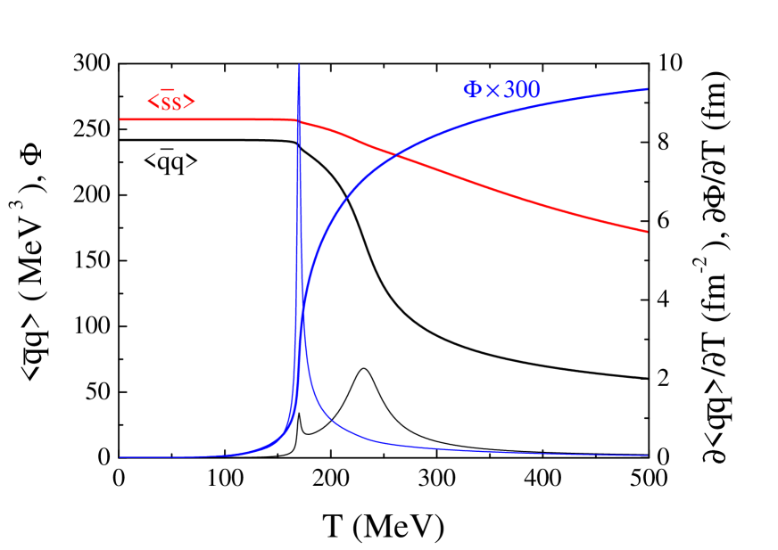
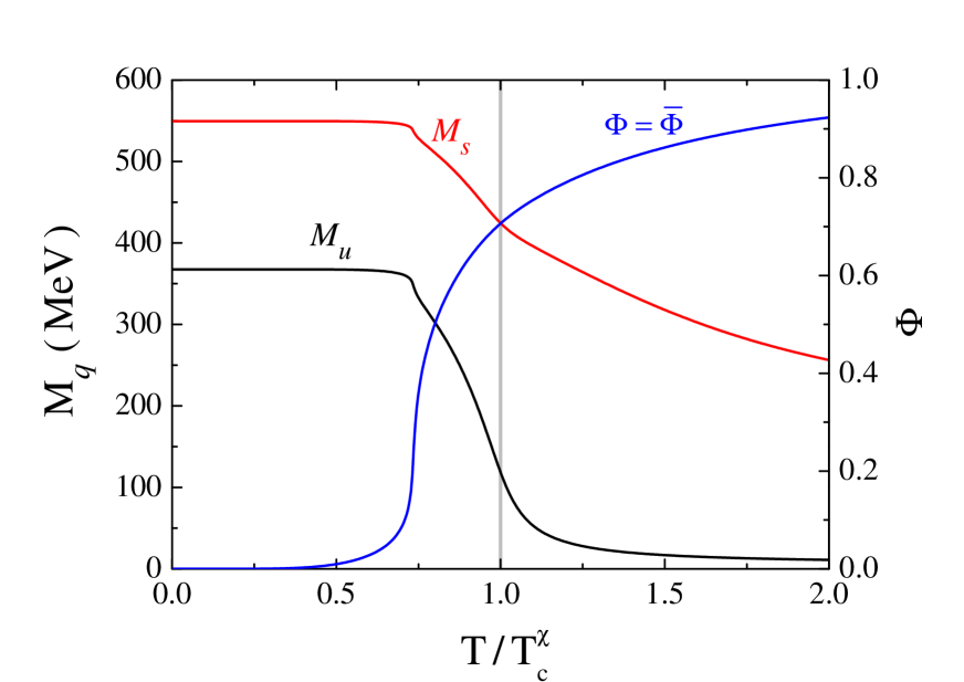
Figure 1: Quark condensates and respective derivatives (left panel) and quark masses (right panel) in the PNJL model as functions of the temperature; the Polyakov loop field, $\Phi$, is also shown, together with its derivative given by the thin blue line in the left panel.

In Table 2, we report the characteristic temperatures in the PNJL model: the pseudocritical temperatures for the chiral transition ($T_{c}^{\chi}$) and deconfinement ($T_{c}^{\Phi}$); the effective chiral symmetry restoration temperature ($T_{eff}^{\chi}$); and the Mott temperatures for pion ($T^{Mott}_{\pi}$), for eta ($T^{Mott}_{\eta}$), for kaon ($T^{Mott}_{kaon}$) and for the sigma ($T^{Mott}_{\sigma}$) mesons. We remind that the Mott transition is related with the composite nature of the mesons: at the Mott temperature it becomes energetically favorable for a meson to decay into a $\overline{q}q$ pair .

Table 2: Characteristic and Mott temperatures in the PNJL model at $\mu_{B}$ with $T_{0}=195$ MeV.

$T_{c}^{\chi}$ [MeV]	$T_{c}^{\Phi}$ [MeV]	$T_{eff}^{\chi}$ [MeV]	$T^{Mott}_{\pi}$ [MeV]	$T^{Mott}_{\eta}$ [MeV]	$T^{Mott}_{K}$ [MeV]	$T^{Mott}_{\sigma}$ [MeV]
$231$	$170$	$280$	$239$	$211$	$243$	$197$

The difference between $T_{c}^{\Phi}$ and $T^{\chi}_{c}$ is due to the choice of $T_{0}$ and the regularization procedure, as it was pointed out in Reference Hansen et al. (2007). In these work a three-dimensional momentum cutoff to both the zero and the finite temperature/densities contributions is applied. Different type of regularizations can lower $T^{\chi}_{c}$ Costa et al. (2008b). In Reference Costa et al. (2010a) the meson properties were calculated without rescaling the parameter $T_{0}$ to a smaller value. By adopting a higher value of $T_{0}$, a smaller difference between the psudocritical temperatures of the two transitions was obtained. However, since our goal is the general properties of mesons, the absolute value of the pseudocritical temperatures is not the most significant point: in fact, these properties are independent of the precise value of $T^{\chi}_{c}$ and different values of $T_{0}$ do not change the conclusions.

III.2 Finite Temperature and Chemical Potential

Now, let’s extend the analysis to the scenario with $\mu_{B}\neq 0$, i.e., the phase diagram. The PNJL model can mimic a region in the interior of a neutron star (where the PNJL model is reduced to the NJL model) or a dense fireball created in a HIC. Bearing in mind that in a relativistic HIC, the fireball evolves rapidly (it takes about $10^{-22}$ s for hadronization), only processes mediated by the strong interaction will attain thermal equilibration rather than the full electroweak equilibrium. In this work, we impose the condition $\mu_{u}=\mu_{d}=\mu_{s}=\mu_{q}$ (equal quark chemical potentials) with $\mu_{B}=3\mu_{q}$. This corresponds to zero charge (or isospin), $\mu_{Q}=0$, and zero strangeness chemical potential, $\mu_{S}=0$. This choice also allows for isospin symmetry, $M_{u}=M_{d}$. The net strange quark density, $\rho_{S}$, will be different from zero but only at very high values of $T$ and/or $\mu_{B}$.

From both panels of Figure 2 one can see that, instead of what happens at finite temperature, at $T=0$ and finite baryonic chemical potential a first-order phase transition takes place with the critical chemical potential being $\mu_{B}^{crit}=1083$ MeV (or $\mu_{q}^{crit}=361$ MeV). As the temperature increases this first-order transition (blue full line) persists up to the chiral CEP (black dot). Along this line, the thermodynamic potential has two degenerate minima which are separated by a finite potential barrier. The two minima correspond to the phases of broken and restored chiral symmetry, respectively. As the temperature increases the height of the barrier decreases and disappears at the CEP, which is located at $T^{CEP}=126.3$ MeV and $\mu_{B}^{CEP}=915.4$ MeV ($\rho_{B}^{CEP}=1.75\rho_{0}$). At the CEP the chiral transition becomes a second-order phase transition.

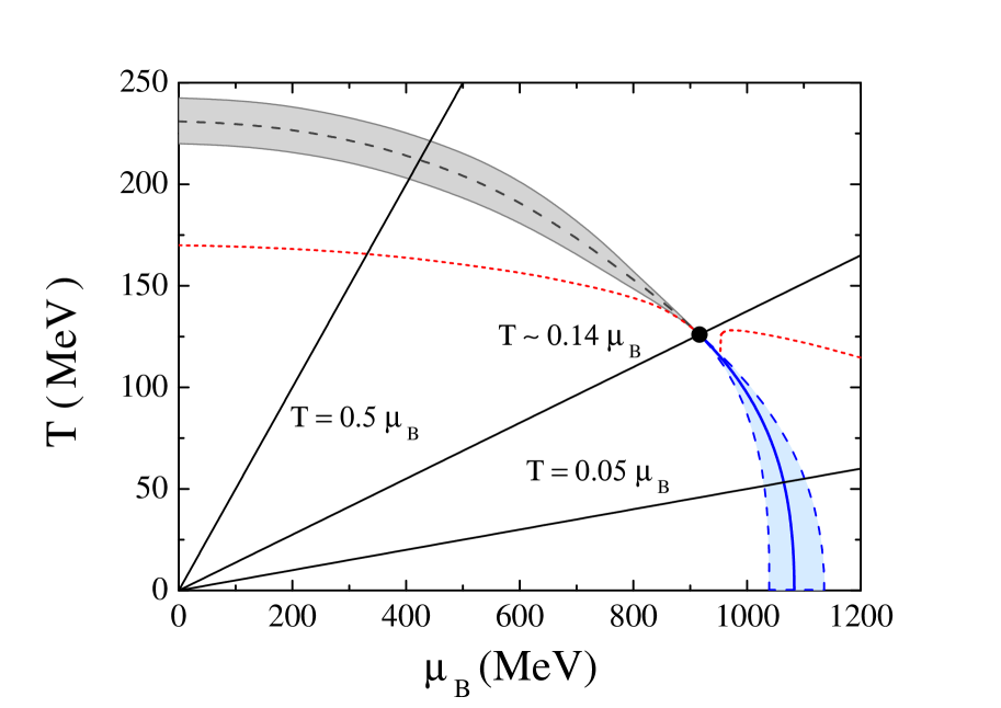
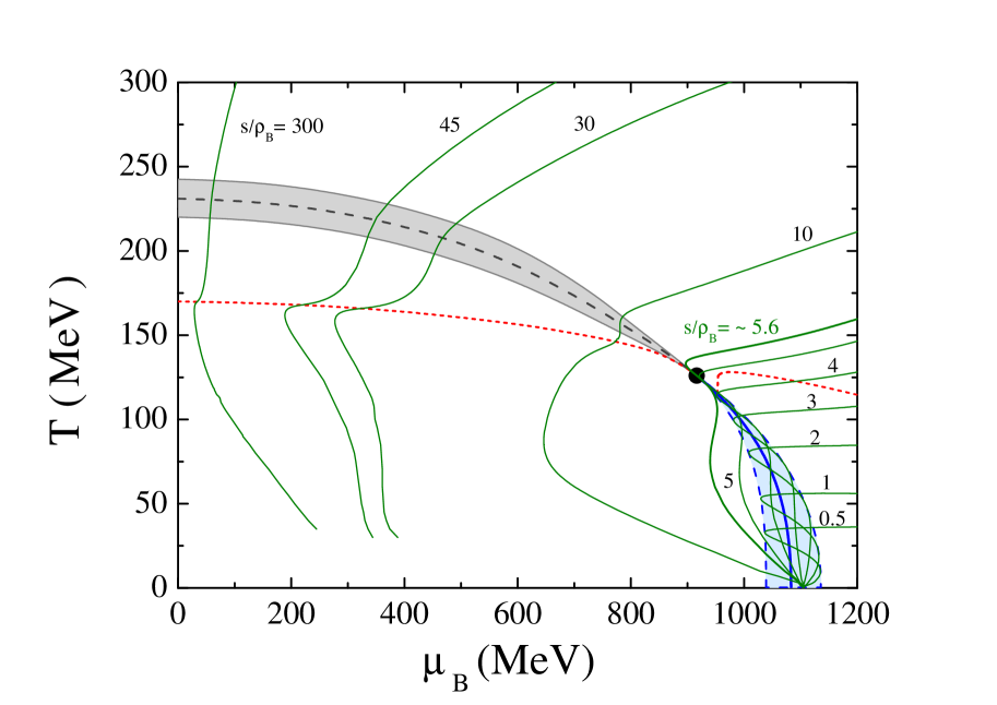
Figure 2: (Left panel) Deconfinement transition (red dots) and chiral transition with first-order (full blue line), CEP (black dot) and crossover regions (dashed black line) and spinodal lines (dashed blue line). (Right panel) Deconfinment and chiral transitions alongside isentropic lines (full green lines).

The blue dashed lines in Figure 2 are the borders of the coexistence area (light blue region). The domain between these lines has metastable states, characterized by large fluctuations. Although they are also solutions of the gap equations, their thermodynamic potential is higher than for the stable solutions. The left dashed curve is the beginning of the metastable solutions of restored symmetry in the phase of broken symmetry, while the right dashed curve depicts the end of the metastable solutions of broken symmetry in the restored symmetric phase. Above the CEP the thermodynamic potential has only one minimum, meaning that the transition is washed out and only a smooth crossover occurs (gray dashed line).

The crossover is a fast decrease of the chiral order-like parameter (the quark condensate) and its range is defined by the interval between the two peaks around the zero of ${\partial^{2}\left\langle\overline{q}_{i}q_{i}\right\rangle}/{\partial T^{2}}$. In Figure 2 this region is presented in gray. It can be seen that, as $\mu_{B}$ increases, the area where the crossover takes place is getting narrower and narrower until it reaches the CEP.

III.3 Nernst Principle and Isentropic Trajectories

It is accepted that the expansion of the QGP in HIC is a hydrodynamic expansion of an ideal fluid and it will nearly follow trajectories of constant entropy. Due to the baryon number conservation, the isentropic trajectories are lines of constant entropy per baryon, i.e., $s/\rho_{B}$, in the ($T,\mu_{B}$)-plane and contain relevant information on the adiabatic evolution of the system. The values of $s/\rho_{B}$ for AGS, SPS, and RHIC, are 30, 45, and 300, respectively Bluhm et al. (2007).

The numerical results for the isentropic trajectories in the $(T,\mu_{B})$-plane are given in the right panel Figure 2. A complete study of the behavior of isentropics trajectories in the PNJL model under the influence of a repulsive vector interaction and by the presence of an external magnetic field was performed in Costa (2016). It is important to start the discussion by analyzing the behavior of the isentropic trajectories when $T\rightarrow 0$. In this limit, $s\rightarrow 0$ according to the third law of thermodynamics and, once also $\rho_{B}\rightarrow 0$, it is insured the condition $s/\rho_{B}\,=\,const.$. In fact, all isentropic trajectories end at the same point ($T=0$ and $\mu_{q}=\mu_{B}/3=367.7$ MeV) of the horizontal axes. Since $\mu_{q}=M_{q}^{vac}>\mu_{q}^{crit}$, the combination ($T=0\,,\mu_{q}=367.7$ MeV) corresponds to the vacuum. With the chosen set of parameters, the point where the first-order transition occurs satisfies the condition $\mu_{q}^{crit}<M_{q}^{vac}$ for $T=0$ Buballa (2005). It also allows the existence of a strong first-order phase transition from the vacuum solution, $M_{q}=M^{vac}_{q}$, into the partially chiral restored phase with $M_{q}$ smaller the $M^{vac}_{q}$. At the transition point, the total baryonic density jumps from zero to $\leavevmode\nobreak\ 2.5\rho_{0}$, equally carried by $u$ and $d$-quarks (the density of strange quarks, $\rho_{s}$, is still zero, and the system only has $\rho_{s}\neq 0$ when $\mu_{q}>M_{s}$).

Close to the first-order region, for $T\neq 0$, the isentropic trajectories ($s/\rho_{B}=1,...,5$) show the following behavior: they come from the region of partially restored chiral symmetry reaching the unstable region (spinodal region), delimited by the spinodal lines, going then along with it as $T$ decreases until they reach $T=0$. By looking to the trajectory $s/\rho_{B}=0.5$, it can be seen that the isentropic trajectory crosses the spinodal line at ($T\approx 36$ MeV, $\mu_{B}\approx 1122$ MeV) and intersects the first-order line twice, at ($T\approx 35$ MeV, $\mu_{B}\approx 1075$ MeV) and ($T\approx 25$ MeV, $\mu_{q}\approx 1080$ MeV), as the temperature decreases in a “zigzag”-shaped trajectory delimited by the spinodal lines. By analyzing the isentropic trajectory with $s/\rho_{B}=5$, it is interesting to notice that it starts by having an identical behavior to the isentropic trajectory $s/\rho_{B}=0.5$, but it then leaves the spinodal region. Nonetheless, as the temperature diminishes, the isentropic trajectory reaches once again the spinodal region, now from lower values of $\mu_{B}$. After that, it also goes to the horizontal axes ($T=0$). The isentrpoic trajectory $s/\rho_{B}=5.6$ nearly goes through the CEP and we will calculate the meson masses along this path.

Concerning the behavior of the isentropic trajectories in the chiral crossover region, ($s/\rho_{B}>5.6$) it is qualitatively similar to the one obtained in lattice calculations Ejiri et al. (2006); Borsanyi et al. (2012b) or in some models Nonaka and Asakawa (2005); Fukushima (2009); Kahara and Tuominen (2008): they directly go through the the crossover region, displaying a smooth behavior. However, they suffer a pronounced bend when they cross the deconfinement transition (red dashed curve) reaching the spinodal region from lower values of $\mu_{B}$. In conclusion, all the trajectories directly arrive in the same point of the horizontal axes at $T=0$.

A final remark; while the critical behavior at the CEP is universal, characteristic shape of the isentropic trajectories near the CEP can change from model to model, even if they belong to the same universality class Nakano et al. (2010).

IV Scalar and Pseudoscalar Mesons in the PNJL Model

In this section, we will study the behavior of scalar and pseudoscalar mesons in the PNJL model for different physical scenarios. We will look for signs of the effective restoration of chiral symmetry and how the chiral transition and the deconfinement affect their behavior. The criterion to identify an effective restoration of the chiral symmetry will be to seek for the degeneracy of the respective chiral partners. Indeed, we will compare the properties (e.g., the masses) of the pseudoscalar meson nonet ($\pi$, $K$, $\eta$, and $\eta^{\prime}$) with those which can be considered as chiral partners, i.e., the scalar mesons ($\sigma$, $\kappa$, $a_{0}$, and $f_{0}$).

IV.1 Mesons Properties at Finite Temperature

IV.1.1 Mesonic Masses and Mixing Angles

We start with the analysis of the mesons and mixing angles general behavior. The plot of the meson masses, mixing angles and coupling constants will be done as functions of the reduced temperature $T/T^{\chi}_{c}$. This will allow a better understanding of their behavior around the chiral pseudocritical temperature. The masses of the pseudoscalar mesons $\pi$, $K$, $\eta$, and $\eta^{\prime}$ (solid lines) and of the respective scalar chiral partners $\sigma$, $\kappa$, $a_{0}$, and $f_{0}$ (dashed lines) as functions of the reduced temperature are given in the left panel of Figure 3.

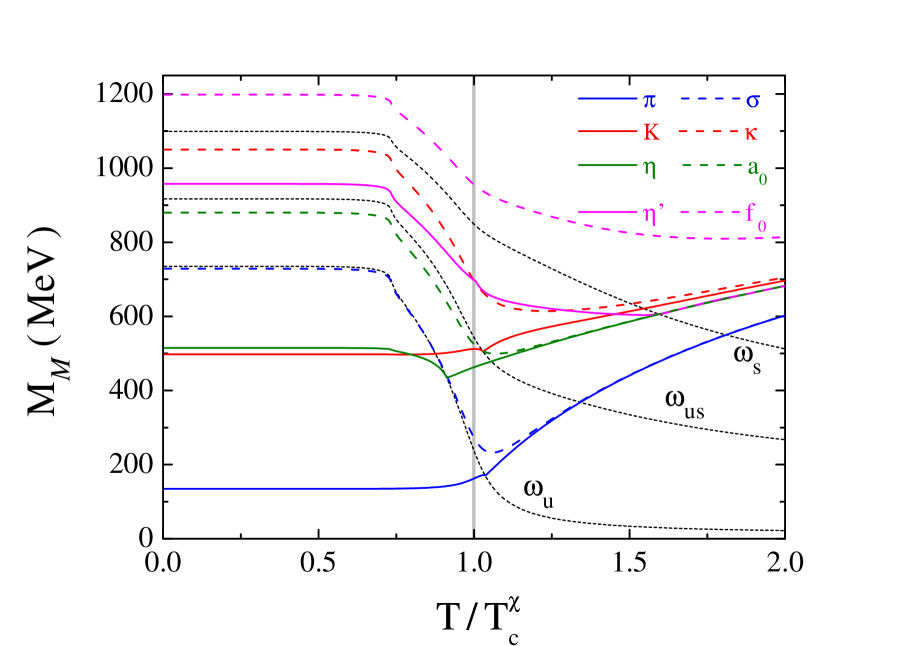
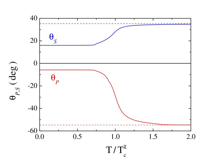
Figure 3: (Left panel) Masses of the pseudoscalar (full lines) and scalar mesons (dashed lines) as function of the reduced temperature. (Right panel) Pseudoscalar and scalar mixing angles as a function of the reduced temperature.

Concerning the pseudoscalar mesons, they are bound states at low temperature (except the $\eta^{\prime}$ meson that is always above the continuum $\omega_{u}=2M_{u}$), but they become unbound at the respective Mott temperatures (see Table 2). The Mott temperature is the temperature where the transition from a bound state to a resonance takes place and, as already pointed out, it comes from the fact that mesons are not elementary objects but composed states of $\overline{q}q$ excitations. Above the Mott temperature, the imaginary parts of the integrals $I_{2}^{ij}$ (see Equation (39)) must be taken into account and the finite width approximation is used Rehberg et al. (1996). The lower limits of the continua belonging to each meson are also shown (black doted lines). Indeed, the continuum starts when the $\pi$, and the $\eta$ masses cross the quark threshold $\omega_{u}=2M_{u}$ and the $K$ crosses $\omega_{us}=M_{u}+M_{s}$. For the $\pi$ and $K$ mesons this entry into the continuum occurs at approximately the same temperature ($T^{Mott}_{\pi}=239$ MeV, $T^{Mott}_{K}=242$ MeV). The $\eta^{\prime}$ meson is always an unbound state and its mass already begins to be larger than $\omega_{u}=2M_{u}$.

Concerning the scalar mesons, the $\sigma$-meson is the only scalar meson that can be considered as a true (slightly) bound state for relatively small temperatures. At the corresponding Mott temperature, $T^{Mott}_{\sigma}=197$ MeV, it turns into a resonance. The other scalar mesons are always resonant states. For the $\pi$, $\eta$ and $\sigma$ there is a second entry into the continuum when the mass of these mesons intersect $\omega_{s}=2M_{s}$.

As shown in Ref. Costa et al. (2010b), at $T^{\chi}_{eff}$ the behavior of some observables signalize the so-called effective restoration of chiral: the masses of the meson chiral partners become degenerated as it can be see in Figure 3 (left panel). In this case, for temperatures above $280$ MeV the $\pi$ starts to be degenerate with the $\sigma$ meson. It also can be seen that the partners [$\pi,\sigma$] (blue curves) and [$\eta,a_{0}$] (green curves) become degenerate at almost the same temperature. In both cases, this behavior is a clear indication of the effective restoration of chiral symmetry in the nonstrange sector. Differently, the masses of $\eta^{\prime}$ and $f_{0}$ mesons do not show a tendency to converge in the range of temperatures considered. This pattern can be interpreted as a sign that chiral symmetry does not show a trend to get restored in the strange sector, a consequence of the slow decrease of $M_{s}$ in Figure 1 (right panel).

Finally, our attention will be focused in the $K$ and $\kappa$ mesons (red curves in the left panel of Figure 3). The $\kappa$ is always unbounded and it exhibits a tendency to get degenerate in mass with the $K$ meson for increasing temperatures.

Summarizing the above, the SU(2) chiral partners [$\pi,\sigma$] and [$\eta,a_{0}$] become degenerate for temperatures higher than $T>280$ MeV (the masses of the $\sigma$ and $\eta$ mesons become less strange, and converge, respectively, with the non strange ones, $\pi$ and $a_{0}$); the [$\eta^{\prime},f_{0}$] do not indicate a tendency to converge in the rage of temperatures studied; the convergence of the partners $K$ and $\kappa$ that have a $\overline{u}s$ structure, occurs at higher values of the temperature, and is presumably slowed down by the small decrease of the strange quark mass, $M_{s}$. The degree of restoration of chiral symmetry in the different sectors essentially drives the mesonic behavior.

It is important to refer that, as pointed out in Costa et al. (2009a), the behavior of the mesonic masses in the PNJL model is qualitatively similar to the corresponding one in the NJL model Costa et al. (2004b, 2003, 2005).

Concerning the pseudoscalar mixing angle, $\theta_{P}$, a first evidence emerges from the right panel of Figure 3: as the temperature increases, it goes to its ideal value $\theta_{P}=$ $-54.736^{\circ}$ asymptotically. As a result, a remarkable change in the quark content of the mesons $\eta$ and $\eta^{\prime}$ occurs, although a small percentage of mixing always remains: the $\eta$ eventually becomes almost nonstrange, while the $\eta^{\prime}$ becomes almost a purely strange meson Costa et al. (2003, 2005). The scalar mixing angle $\theta_{S}$ shows an identical tendency: the ideal mixing angle goes asymptotically to $\theta_{S}=$ $35.264^{\circ}$. Therefore, there is a decrease of the strange component of the $\sigma$-meson, that never disappears, and $f_{0}$ becomes almost purely strange.

The mixing angles are very sensitive to temperature (and also the medium) effects, particularly due to its influence on the mass of strange quark. This might be an explanation to the fact that some aspects of $\theta_{S}$ and $\theta_{P}$ behavior are not the same in different models Schaefer and Wagner (2009); Horvatic et al. (2007). It should be noticed that the mixing angles depend on the mesons masses, namely, $\theta_{S}$ on the mass of the $\sigma$-meson and $\theta_{P}$ on the mass of the $\eta$-meson.

The evolution of the strangeness content of both mesons, $\eta$ and $\eta^{\prime}$ determines which meson will become nonstrange, and consequently will behave as the chiral axial partner of the $\pi$. The behavior of $\theta_{P}$ at finite temperature leads to the identification of the $\eta$ as the chiral axial partner of the $\pi$, but the opposite is found in References Lenaghan et al. (2000); Schaefer and Wagner (2009) where a crossing of the mixing angles can be seen. A certain degree of crossing of the pseudoscalar mixing angle and exchange of identities of $\eta,\,\eta^{\prime}$ was also seen in Reference Schaffner-Bielich (2000), and an alike effect for the scalar angle was presented in Ref. Schaefer and Wagner (2009). Indeed, because of the mixing angles behavior, $f_{0}$ and $\eta^{\prime}$ become essentially strange for increasing temperatures. Besides, as it was shown in Reference Costa et al. (2008b), even when the spontaneously broken chiral symmetry gets restored in all sectors (and unlike what is found for the nonstrange chiral partners) a considerable difference between the masses of these mesons is still present, a fact due to the high value of the current strange quark mass used in this work ($m_{s}=140.7$ MeV). Indeed, at high temperatures the relation $m_{f_{0}}^{2}\simeq m_{\eta^{\prime}}^{2}+4m_{s}^{2}$ is approximately valid, thus explaining the observed behavior.

IV.1.2 Pion and Kaon Coupling Constants

The left(right) panel of Figure 4 shows the values of the $\pi$ and $K$ coupling(decay) constants. At the Mott temperature, a striking behavior for each meson can be seen: the coupling strengths approach zero for $T\rightarrow T_{\pi(K)}^{Mott}$ Rehberg et al. (1996). This behavior occurs because the polarization displays a kink singularity, which can also be seen in the meson masses.

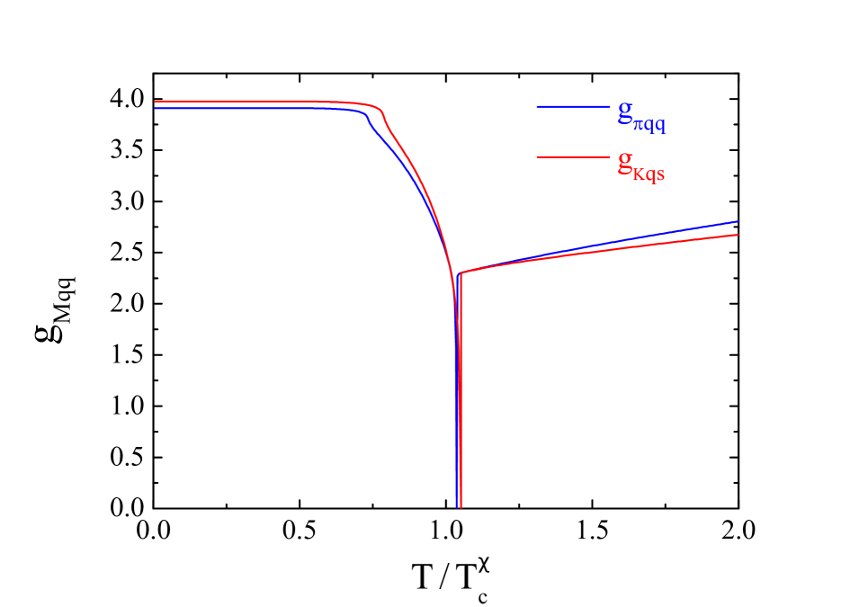
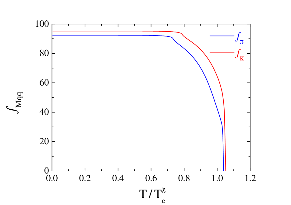
Figure 4: Coupling constants (left panel) and decay constants (right panel) as a function of the reduced temperature.

It is interesting to note that the Mott temperature for each meson is above $T^{\chi}_{c}$, indicating a slightly survival of these mesons as bound states in the restored phase. This is a feature of the PNJL model, which is a quantitative step toward confinement regarding the NJL model. This is due to the $\Phi$ factor that suppresses the 1- and 2- quarks Boltzmann factor at low temperatures. Indeed, the fast restoration of the $\mathbb{Z}_{3}$ symmetry ($\Phi$ goes to one with increasing temperatures) produces a quark thermal bath with all (1-, 2- and 3-) quark contributions in a short range of temperatures, which might help to explain the fastening of the transition Costa et al. (2009a).

IV.2 Mesons at Zero Temperature

Next, we will study the meson behavior at finite values of $\mu_{B}$. We emphasize that, as previously stated, the employed PNJL model at $T=0$ is identical to the usual NJL model.

We consider symmetric quark matter as in Section III.2. The first aspect that arises is that, similarly to the previous finite temperature scenario, chiral symmetry is effectively restored only in the light sector. This is due to some specific details of the behavior of the strange quark mass with the density. Figure 5 shows the quark masses as function of $\mu_{B}$ around the first-order transition, left panel, and as a function of $\rho_{B}/\rho_{0}$, right panel (the light-blue area corresponds to the region of the phase transition). As it can be seen, in the present case there are no strange quarks in the medium at low densities. The mass of the strange quark smoothly decreases, due to the effect of the ’t Hooft interaction, and it becomes smaller than the chemical potential for strange quarks (at $\rho_{B}\simeq 5.45\rho_{0}$ and $\mu_{B}\simeq 1388$ MeV) and strange quarks appear in the system. Then, a pronounced decrease of the strange quark mass is observed.

With respect to the meson spectra and the mixing angles, we will discuss new aspects that arise, mainly in the high baryonic chemical potential/density region.

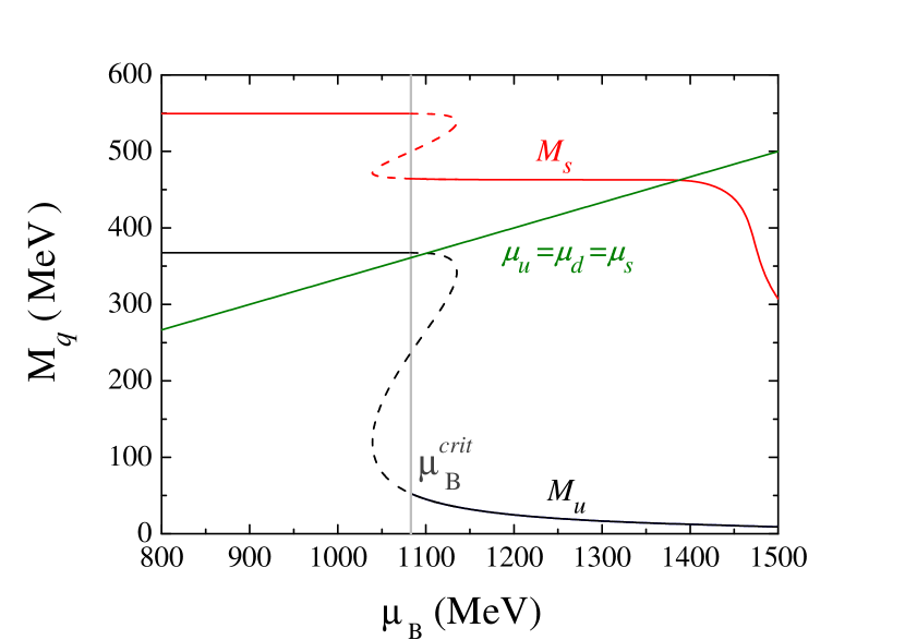
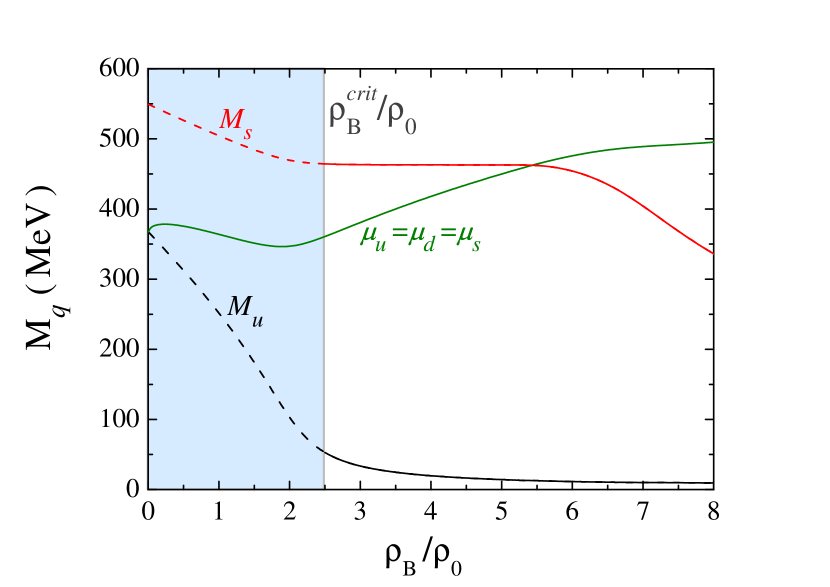
Figure 5: Quark masses at $T=0$ as a function of the baryonic chemical potential (left panel) and reduced baryonic density (right panel). The dashed lines represent the quark masses in the first-order region. $\mu_{B}^{crit}$ is the baryonic critical chemical potential of the first-order phase transition, and $\rho_{B}^{crit}/\rho_{0}$ the respective critical reduced density ($\rho_{0}=0.16$ fm^-3).

In Figure 6, the meson masses are plotted as functions of the baryonic chemical potential (panel (a)) and of the density (panel (b)). The chiral partners [$\pi,\sigma$] (blue curves) are always bound states. Before continuing the discussion, some words about the continuum $\omega^{\prime}$ at zero temperature are needed. From the dispersion relations for the pion and kaons, at $T=0$, two kinds of discrete bound states are allowed (looking to the limits of the regions of poles in the integrals $I^{ij}_{2}$, Equation (39)): particle-antiparticle modes of the Dirac sea, that are already present in the vacuum and are related with the spontaneous breaking of chiral symmetry; and, when the breaking of the flavor symmetry is considered, particle-hole excitations of the Fermi sea, that only manifest themselves in the medium (for a detailed description, see de Sousa and Ruivo (1997)). On the other hand, the Fermi and Dirac sea continua are defined by the unperturbed solution. In the isospin limit, the Dirac continuum starts at $\omega^{\prime}=\omega_{u(d)}^{\prime}=2\mu_{u(d)}$ and at $\omega_{s}^{\prime}=2\mu_{s}$ (at finite temperature, we have $\omega_{u(d)}=2M_{u(d)}$, and $\omega_{s}=2M_{s}$).

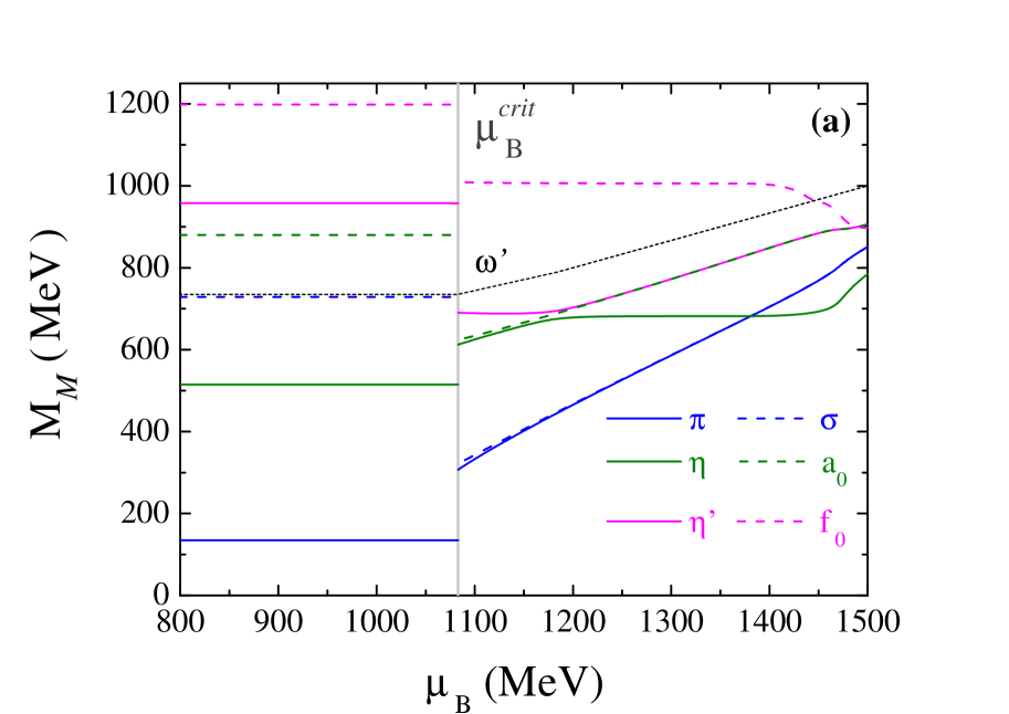
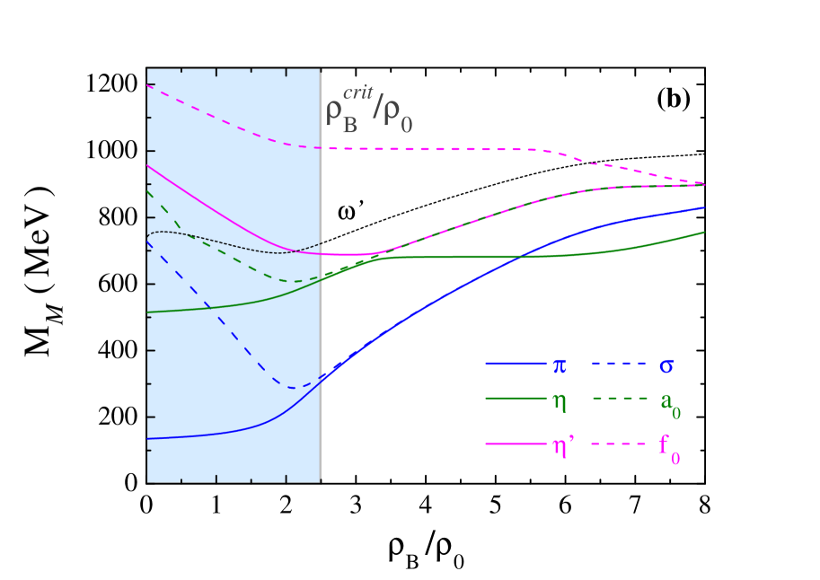
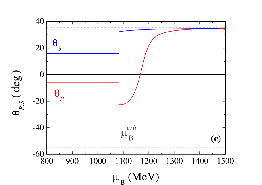
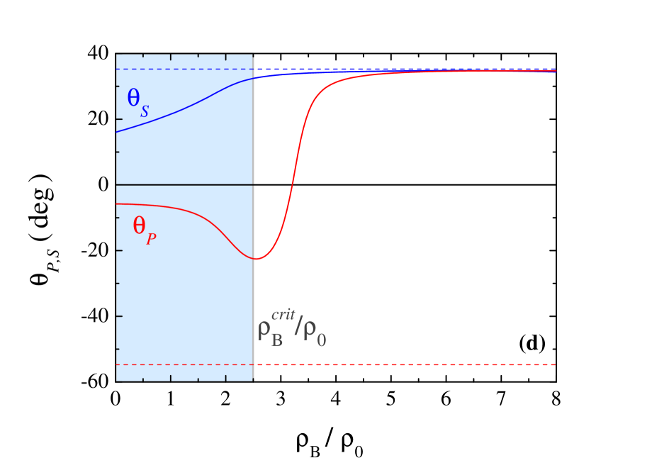
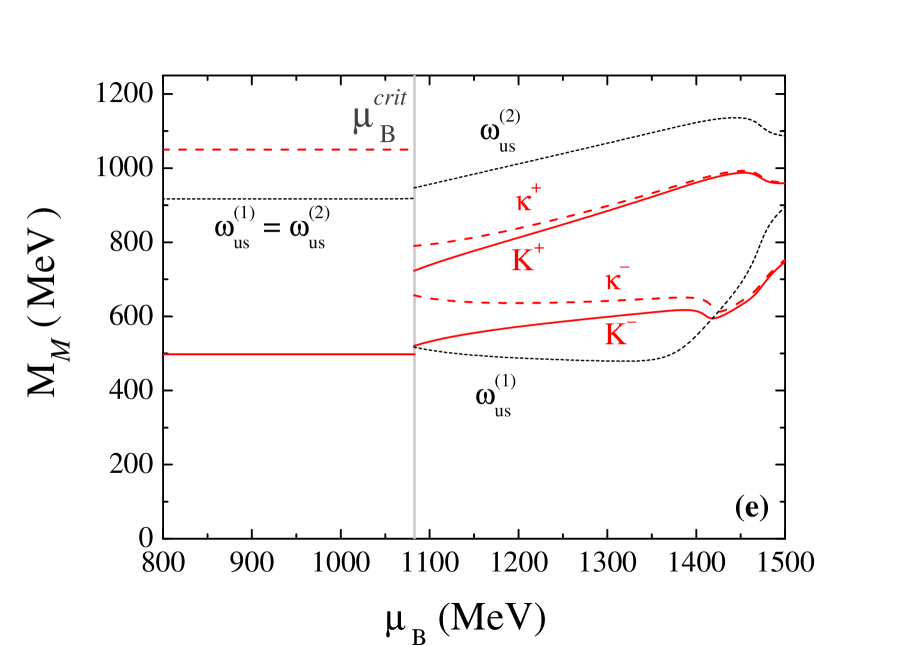
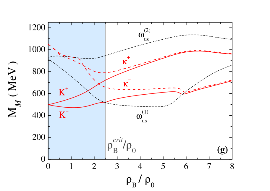
Figure 6: Masses of the neutral pseudoscalar and scalar mesons as a function of $\mu_{B}$ (panel (a)) and as a function of $\rho_{B}/\rho_{0}$ (panel (b)); the pseudoscalar and scalar mixing angles as a function of $\mu_{B}$ (panel (c)) and as a function of $\rho_{B}/\rho_{0}$ (panel (d)); masses of the charged pseudoscalar and scalar mesons as a function of $\mu_{B}$ (panel (e)) and as a function of $\rho_{B}/\rho_{0}$ (panel (g)). All results are at $T=0$ (see text for details).

Returning to meson masses, for all range of densities (chemical potentials), the pion is a light quark system contrary to the $\sigma$ meson which has a strange component at $\rho_{B}=0$ but never becomes a purely non-strange state because $\theta_{S}$ never reaches the ideal mixing angle $35.264^{\circ}$ (Figure 6, panels (c) and (d)). As $\rho_{B}$ ($\mu_{B}$) increases these mesons become degenerate ($\rho^{eff}_{B}\gtrsim 2.9\rho_{0}$, $\mu_{B}^{eff}\gtrsim 1126$ MeV, effective restoration of chiral symmetry in the light sector, see blue curves of panels (a) and (b)).

At the approximate same density, and $\mu_{B}$, the chiral partners [$\eta,a_{0}$] (green curves in panels (a) and (b) of Figure 6) also become degenerate. On one hand, the $\eta$-meson is permanently a bound state; on the other hand, $a_{0}$ starts to be a resonance, because its mass is above the $\overline{q}q$ continuum, and converts into a bound state for $\rho_{B}\gtrsim 0.6\rho_{0}$, and $\mu_{B}\gtrsim 1121$ MeV.

However, as the baryonic chemical potential (panel (a)) or the density (panel (b)) increases, the $a_{0}$ mass splits from the $\eta$ mass and goes to degenerate with the $\eta^{\prime}$ mass. To clarify this behavior we look to the behavior of the mixing angle $\theta_{P}$ in panels (d) and (e) of Figure 6: it is noticed that the angle $\theta_{P}$, which starts at $-5.8^{\circ}$, changes sign at $\mu_{B}\simeq 1167$ MeV ($\rho_{B}\simeq 3.2\rho_{0}$) becoming positive and increasing rapidly, which can be interpreted as a signal of a change of identity between both $\eta$ and $\eta^{\prime}$ mesons. As it was seen in Figure 5, the strange quark mass decreases more rapidly when strange quarks appear in the system ($\mu_{q}>M_{s}$). A consequence of this behavior is the changing in the percentage of strange, $(q\overline{q})_{s}=s\overline{s}$, and non-strange, $(q\overline{q})_{\rm ns}=\frac{1}{2}({u}\overline{u}+{d}\overline{d})$, quark content in $\eta$ and $\eta^{\prime}$ mesons: the $\eta^{\prime}$ has a bigger strangeness component than the $\eta$ at low density, and the opposite takes place at high density Costa et al. (2003). Then, the $\eta^{\prime}$ mass will degenerate with the mass of the $a_{0}$-meson that is permanently a non-strange state. As a final point, the $f_{0}$-resonance is a strange state for all densities that denotes a tendency to be degenerated with other mesons only at very high values of $\mu_{B}$ ($\rho_{B}$).

A very interesting scenario happens for kaons and their chiral partners: $K^{\pm}$ and $\kappa^{\pm}$ (Figure 5, panels (e) and (f)). A first finding concerns to the separation between charge multiplets of kaons and the respective $\kappa$-mesons. Also the the mass degeneracy of [$K^{+}$, $\kappa^{+}$] and [$K^{-}$, $\kappa^{-}$] occur at different values of density (chemical potential) which are higher then for [$\pi,\sigma$]. Indeed, taking the difference ($M_{K^{\pm}}-M_{\kappa^{\pm}}$), now at $5\%$ of its vacuum value, for [$K^{+}$, $\kappa^{+}$] the degeneracy of their masses takes place at $\mu_{B}=1187$ MeV ($\rho_{B}=3.38\rho_{0}$) while for [$K^{-}$, $\kappa^{-}$] the degeneracy takes place at $\mu_{B}=1419$ MeV ($\rho_{B}=5.86\rho_{0}$).

Another particularity is the fact that the $K^{+}$ is always a bound state, never reaching the continuum, while the $K^{-}$ is bounded only until it gets in the continuum of $s\overline{u}$ excitations of the Dirac sea at $\mu_{B}=1083$ MeV ($\rho_{B}=2.5\rho_{0}$) and becomes thereafter a $s\overline{u}$ resonance: $M_{K^{-}}>\omega_{us}^{(1)}$ (with $\omega_{us}^{(1)}=(M_{s}^{2}+\lambda_{u}^{2})^{1/2}+\mu_{u}$, being the chemical potential $\mu_{u}=(M_{u}^{2}+\lambda_{s}^{2})^{1/2}$, and the Fermi momentum of the $i$-quark $\lambda_{i}=(\pi^{2}\rho_{i})^{1/3}$). However, when $\mu_{B}>1419$ MeV ($\rho_{B}>5.85\rho_{0}$) the $K^{-}$ becomes once again a bound state (this behavior was already found in Costa and Ruivo (2002); Costa et al. (2004b)). Still as far as the $K^{-}$ is concerned, it was shown in Ruivo and de Sousa (1996); de Sousa and Ruivo (1997); Costa and Ruivo (2002); Costa et al. (2005) that there are low bound states with quantum numbers of $K^{-}$ that appear below the inferior limit of the Fermi sea continuum of particle-hole excitations being the Fermi see bounded by $\omega_{low}=(M_{s}^{2}+\lambda_{u}^{2})^{1/2}-\mu_{u}$ and $\omega_{up}=(M_{s}^{2}+\lambda_{s}^{2})^{1/2}-(M_{u}^{2}+\lambda_{s}^{2})^{1/2}$. However, we will not go further in this discussion.

Finally, with respect to the scalar mesons, $\kappa^{\pm}$, it is verified that both mesons start to be unbounded, with the continuum now defined as $\omega_{us}^{(2)}=\mu_{s}+(M_{u}^{2}+\lambda_{s}^{2})^{1/2}$ (at $T=\rho_{B}=0$ $\omega_{us}^{(1)}=\omega_{us}^{(2)}$) but, as $\mu_{B}$ ($\rho_{B}$) increases, they will turn into bound states and become degenerated with the respective partners.

IV.3 Mesons Properties in Different Regions of the Phase Diagram

IV.3.1 Meson Masses in the Crossover Region

We continue the analysis of the behavior of mesons masses in symmetric matter, by following a path in the ($T-\mu_{B}$)-plane passing through the crossover region. As indicated in Figure 2, we choose the path $T=0.5\mu_{B}$. Chiral symmetry is, again, effectively restored only in the light quark sector. In Figure 7 the meson masses are plotted as functions of temperature and baryonic chemical potential, in the left panels and right panels, respectively.

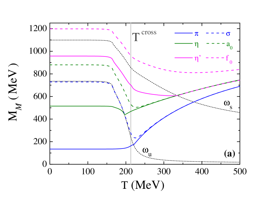
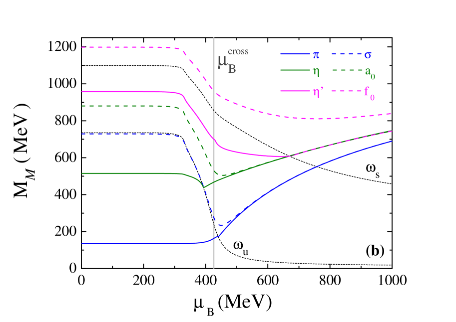
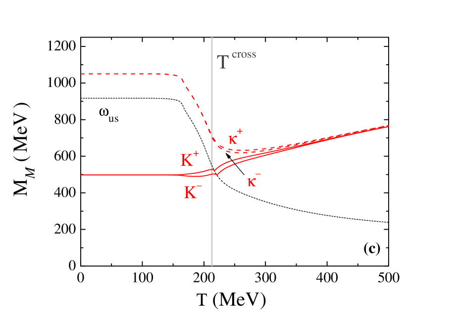
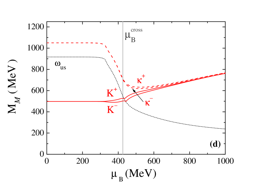
Figure 7: Masses of the pseudoscalar and scalar mesons as function of the temperature (panels (a,c)) and as function of $\mu_{B}$ (panels (b,d)) along the path $T=0.5\mu_{B}$, the crossover region. $T^{\text{cross}}=213$ MeV and $\mu_{B}^{\text{cross}}=426$ MeV are, respectively, the temperature and the baryonic chemical potential for the crossover.

The chiral partners [$\pi$,$\sigma$] and the $\eta$ meson are bound states up to the respective Mott dissociation for a certain temperature and chemical potential(density) as can be seen in panels (a) and (b) Figure 7. The pion still survives as a bound state after the crossover transition in a small range of temperatures and chemical potentials.

Differently from the zero temperature case, and like the case at finite temperature and zero density, the $a_{0}$ meson is always a resonance since its mass always lies above the $\omega_{u}=2M_{u}$ continuum (see Figure 7 panel (a) and (b)). As in the zero temperature case, the degeneracy between each set of chiral partners, [$\pi$,$\sigma$] and [$\eta$,$a_{0}$], happens at almost the same temperature and chemical potential.

The $\eta^{\prime}$ meson is always a resonate state and it will reach the $\omega_{s}=2M_{s}$ continuum, a temperature and a chemical potential where it can decay also in a $\overline{s}s$ pair. Immediately, it degenerates with the $\eta$ and $a_{0}$ mesons. Its chiral partner, $f_{0}$, is always above the $\omega_{s}=2M_{s}$ continuum.

Concerning the kaons and their chiral partners (Figure 7, panels (c) and (d)), the previously observed charge splitting at $T=0$ MeV is also present (contrasting with the case $\mu_{B}=0$ MeV where no splitting occurs). However, its effect is much less visible then in the zero temperature case and it happens, for the $K^{\pm}$, before the crossover while for $\kappa^{\pm}$ it happens after the critical temperature and chemical potential. Both $K^{+}$ and $K^{-}$ are bound states until they reach the $\omega_{us}=M_{u}+M_{s}$ continuum while their chiral partners, are always resonances. The continuum is reached slightly above the critical temperature and baryonic chemical potential of the crossover transition.

The degeneracy mechanism for these mesons in this path is different from previously studied zero temperature case. Since the charge splitting in this scenario is much less severe, we first observe degeneracy between each charge multiplet $K^{\pm}$ and $\kappa^{\pm}$, happening at approximately the same temperature and chemical potentials. Following this behavior the chiral partners [$K$,$\kappa$] become degenerate at higher values of temperature and baryonic chemical potential.

At high enough temperatures and chemical potentials (outside the range of applicability of the model) it is expected that all mesons become degenerate.

IV.3.2 Mesons through the CEP

In this subsection we explore the meson behavior along a path that goes through the CEP. This path can be parameterized by $T=0.14\leavevmode\nobreak\ \mu_{B}$, as seen in Figure 2. The meson masses are plotted as functions of temperature and chemical potential, in the left panels and right panels of Figure 8 respectively.

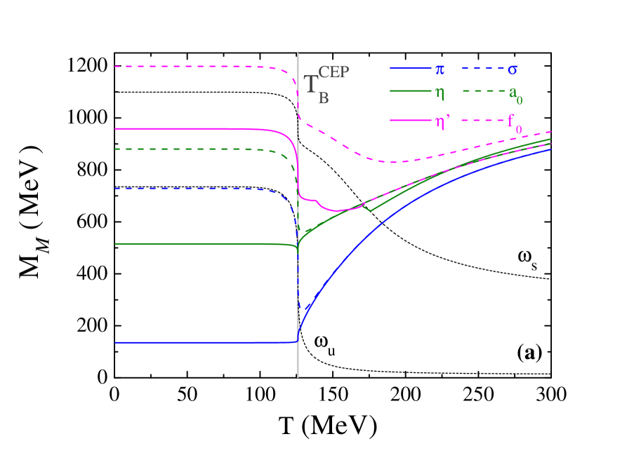
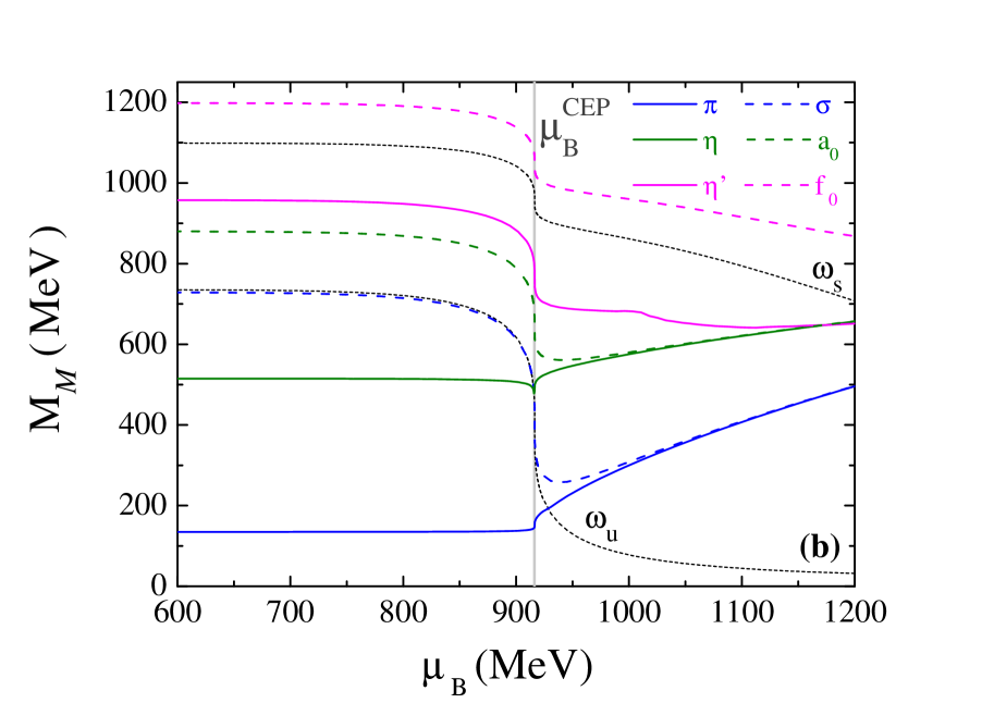
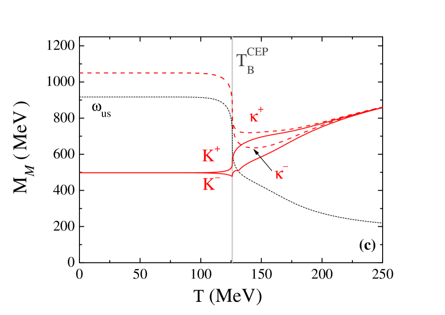
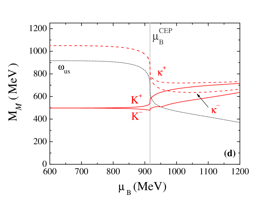
Figure 8: Masses of the pseudoscalar and scalar mesons as function of the temperature (panels (a,c)) and as function of $\mu_{B}$ (panels (b,d)) along the path that crosses the CEP.

We first discuss the behavior of the [$\pi$,$\sigma$], [$\eta$,$a_{0}$] and [$\eta^{\prime}$,$f_{0}$] meson masses presented in panels (a) and (b) of Figure 8. The main and most important observation from Figure 8 is the drastic continuous decrease that almost meson masses (except the pion and $K^{+}$) displays in the temperature and chemical potential of the CEP. In fact, this feature may be used as a signal for the CEP. For example, processes such as $\sigma\rightarrow\pi\pi$ and $\sigma\rightarrow\gamma\gamma$ productions are important tools for the search of the CEP Anticic et al. (2010); Hatsuda et al. (1999). If the $\sigma$-meson has an abnormally small mass around the CEP, this means that peculiar experimental signatures are expected to be observed through its spectral changes: the dipion decay can be suppressed near the CEP due to the fast reduction of the $\sigma$-meson mass. Also the maximum in the $K^{+}/\pi^{+}$ ratio (“the horn” effect) Cleymans et al. (2005), that was discussed as a possible signal of the onset of deconfinement, that also appears near CEP (being considered as a critical region signal for the CEP Friesen et al. (2018)), can be related with the increase of the $K^{+}$ mass seen in Figure 8 (panels (c) and (d)) relative to the decreasing $K^{-}$ mass.

The $\sigma$ and $\eta$ mesons are bound states up to the CEP, where both mesons reach the $\omega_{u}$ continuum. The pion survives as a bound state after the CEP for a very limited range of temperatures and chemical potentials, reaching the continuum after the CEP. After becoming resonances, the chiral partners [$\pi$,$\sigma$] degenerate. The $\eta^{\prime}$-meson mass is bigger then the $\omega_{u}$ continuum, meaning it is always unbound. The [$\eta$,$a_{0}$] also become degenerate up to the $\omega_{s}$ continuum where the $\eta$ (green curve) and $\eta^{\prime}$ (magenta curve) switch roles (this is particularly seen in panel (a) of Figure 8 with the mesons as functions of the temperature), as we will discuss in the following. The $f_{0}$ meson is a resonance and its mass is always above the $\omega_{s}$ continuum.

The $\eta^{\prime}$ mass reaches the $\omega_{s}$ continuum at $\sim 1.4T^{\mathrm{CEP}}$ and $\sim 1.4\mu_{B}^{\mathrm{CEP}}$. Then, the $\eta$ and $\eta^{\prime}$ switch nature since the $\eta^{\prime}$ immediately become degenerate with the $a_{0}$ meson while the $\eta$ meson separates from the $a_{0}$ mass and asymptotically degenerates with the $f_{0}$ meson mass.

As in the crossover scenario, there is charge splitting before and after the CEP for the $K^{\pm}$ and $\kappa^{\pm}$, respectively (see panels (c) and (d) of Figure 8). The splitting for kaons become even more pronounced just at the CEP. The $K^{+}$ is a bound state up to the CEP where it reaches the $\omega_{us}$ continuum while the $K^{-}$ is a bound state that survives the CEP, for a limited range of temperature and chemical potential. After becoming resonances, the both kaons will degenerate with the respective chiral partners of the same charge, $\kappa^{\pm}$, being these scalar mesons always resonances. The charge splitting between mesons disappears as temperature and chemical potential increases (faster for the temperature).

IV.3.3 Mesons through the First-Order Transition

We now analyze a path that goes through the first-order phase transition, parameterized by $T=0.05\leavevmode\nobreak\ \mu_{B}$ (see Figure 2). In the right and left panels of Figure 9, are displayed the mesons masses as functions of the temperature and chemical potential for this scenario.

The general behavior of the mesons in this case is very similar to the one encountered in the zero temperature case since, in both cases, there is a first-order phase transition. However, there are some specifications.

The $\pi$, $\sigma$ and $\eta$ mesons are bound states up to the phase transition. Immediately after this point they, discontinuously, become resonances. In fact, the discontinuity in the meson masses is a consequence of the nature of the first-order phase transition where the thermodynamical potential has two degenerate minima and there is a discontinuous jump from one stable minimum to the other. The $a_{0}$ meson is always a resonance.

The $\eta^{\prime}$ meson mass is always above $\omega_{u}$ up to the point where it reaches the $\omega_{s}$ continuum at higher values of temperature and chemical potential. The $f_{0}$ meson is also always unbound with its mass above $\omega_{s}$.

After the first-order phase transition the pairs $\pi$ and $\sigma$ and $\eta$ and $\eta^{\prime}$ degenerate almost immediately. When the $a_{0}$ mass (dashed green curve) reaches the mass of the degenerate $\eta$ and $\eta^{\prime}$ pair, the $\eta$-meson (solid green curve) decouples from the $\eta^{\prime}$. After this point, the $\eta^{\prime}$ and $a_{0}$ degenerate and evolve to degenerate with the $f_{0}$ meson at high energies while, the $\eta$-meson, remains separate from the [$\eta^{\prime}$,$a_{0}$] pair. When the $\eta$ mass reaches the $\omega_{s}$ continuum its mass increases to asymptotically degenerate with the other mesons.

Regarding the kaons and their chiral partners, right before the first-order phase transition the charge multiplets of the $K$ start to split (see Figure 9 panels (c) and (d)). Before the phase transition only the $K$ mesons are bound while the chiral partners, $\kappa$, are resonances. At the first-order phase transition, as expected, there is a discontinuous split of each charge multiplet of both $K$ and $\kappa$ and every meson is now a resonance, since they all lie above the $\omega_{us}$ continuum. As temperature and chemical potential increases, the $K^{+}$ and $\kappa^{+}$ mesons start to degenerate, followed by the respective negative pair. For larger energies the charge multiplets of the chiral pair also show tendency to degenerate.

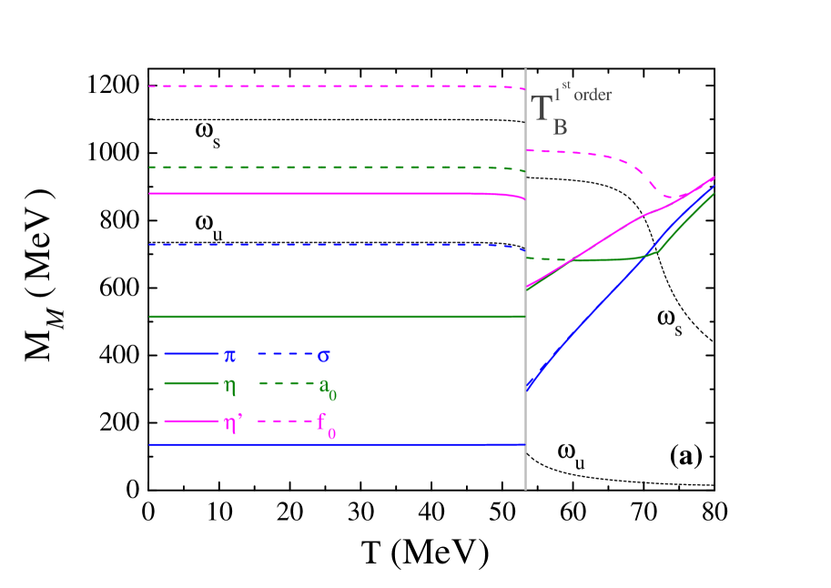
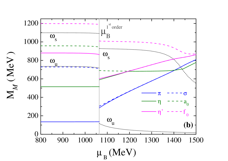
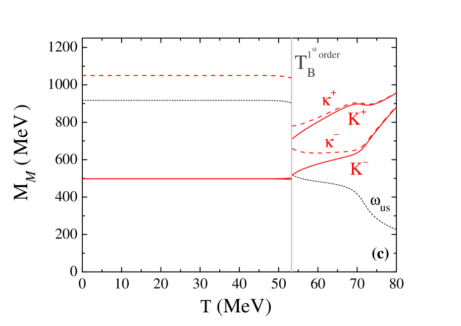
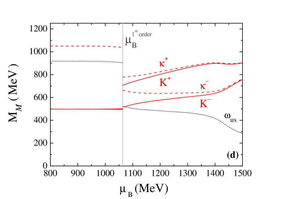
Figure 9: Masses of the pseudoscalar and scalar mesons as function of the temperature (panels (a,c)) and as function of $\mu_{B}$ (panels (b,d)) along the the path $T=0.05\mu_{B}$, crossing the first-order region.

IV.3.4 Mesons along the Isentropic Trajectory That Passes over the CEP

Previously, the isentropic trajectories relevance was presented, namely the fact that the expansion of the QGP in HIC is accepted to be a hydrodynamic expansion of an ideal fluid and it approximately follows trajectories of constant entropy. This argument motivates the presentation of the behavior of mesons masses as functions of the temperature along the nearest isentropic trajectory of the CEP, $s/\rho_{B}\approx 5.6$, in Figure 10. There is a substantial difference for the scenario studied in Section IV.3.2 (the path $T=0.14\mu_{B}$): the abrupt decrease of the meson masses is not seen. Indeed, in this case, along the isentropic trajectory both, the temperature and the baryonic chemical potential, are varying in such a way that $s/\rho_{B}$ is held constant. So, the approximation to the CEP is not direct, being the behavior of the mesons masses more smooth in the neighborhood of the CEP. This may be an indication of different critical behavior near the CEP, depending on the direction the CEP is approached in the $(T,\mu_{B})$ plane. Indeed in Costa et al. (2009b), the critical exponents in the PNJL model were studied and it was found that their values slightly changed depending on the direction. Nevertheless, from the right panel of Figure 10, we see that the separation between $K^{+}$ and $K^{-}$ is the same ($\sim 70$ MeV) like in Section IV.3.2, as it should.

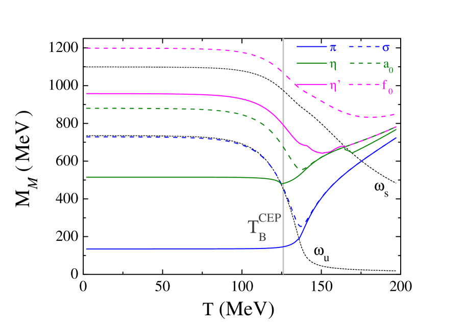
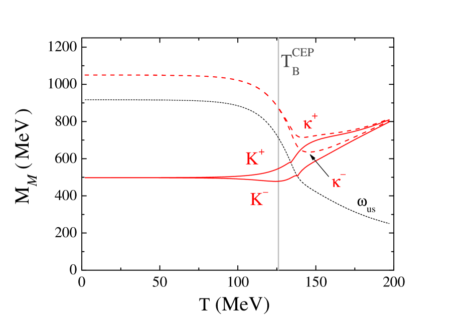
Figure 10: Masses of the pseudoscalar and scalar mesons as function of the temperature (left panel) and as function of $\mu_{B}$ (right panel) along the the path $T=0.05\mu_{B}$, crossing the first-order region.

IV.4 Effective Restoration of Chiral Symmetry and Mott Dissociation of $\pi$ and $\sigma$ along the Phase Diagram

Since the pion and the sigma mesons dissociate in a $\overline{q}q$ pair, in Figure 11 we represent the respective “Mott lines”. In the region $\mu_{B}<\mu_{B}^{CEP}$, the Mott line for $\sigma$-meson occurs below chiral crossover, while the correspondent Mott line for $\pi$ occurs slightly above. It is interesting to note that above $\mu_{B}\sim\mu_{B}^{CEP}$ both Mott lines occurs inside the first-order region.

When we use the degeneracy of the $\pi$ and $\sigma$-meson masses as criterion to define the point of the effective restoration of chiral symmetry, we guarantee that all quantities that violate the chiral symmetry are already sufficiently small. We then can draw a line for the effective restoration of chiral symmetry (brown line in Figure 11). For example, when finally $M_{\pi}=M_{\sigma}$, the constituent masses of the $u$ and $d$ quarks are already sufficiently close to the respective currents masses values (also the light quark condensates already have a very low values).

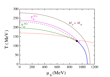
Figure 11: Line of effective restoration of chiral symmetry (brown curve) and the Mott dissociation line for $\pi$ (magenta) and $\sigma$ (green) along the ($T-\mu_{B}$)-plane.

V Conclusions

In this work, we have explored the phase diagram of strongly interacting matter and discussed the scalar-pseudoscalar meson spectrum, with related properties, in connection with the restoration of chiral symmetry and deconfinement for different regions of the phase diagram. We have used the (2 + 1) PNJL model with explicit breaking of the U_A(1) anomaly, which includes flavor mixing, and the coupling of quarks to the Polyakov loop. The PNJL model has proven to be very useful in understanding the underlying concepts of the phase diagram of strongly interacting matter, namely the chiral symmetry breaking and restoration mechanisms. It is also an important tool to study the dynamics of pseudoscalar and scalar mesons with regard to the effective restoration of chiral symmetry.

Some of the presented results have shown a great relevance:

1. the survivability of some meson modes, especially the pion, as a bound state after the transition to the QGP (this tendency to a slightly longer survival as bound state is also shown by the behavior of meson-quark coupling constants for $\pi$, $\sigma$ and $\eta$ mesons);

2. the change of identity between $\eta$ and $\eta^{\prime}$ at finite density for scenarios at lower temperatures;

3. the meson masses change abruptly when choosing a path that passes through the CEP (this can be very important for the signatures of the CEP);

4. in relation to kaons, with the exception of the limiting cases for $T=0$ and $\mu_{B}=0$, a kaon charge splitting before critical temperature/baryonic chemical potential occurs. At CEP and first-order cases, kaons first degenerate with the respective chiral partners and only then with charge multiplet, contrary to the crossover scenario where charge multiplets degenerate first. At the CEP, there is a accentuated splitting for kaons, with $K^{+}$ sharply increasing, a splitting that is still pronounced just after the CEP;

5. above certain critical values of temperature and chemical potentials ($T^{\chi}_{eff}$, ${\mu_{B}}_{eff}^{\chi}$) the masses of the chiral partners [$\pi$,$\sigma$] will degenerate, meaning that chiral symmetry is effectively restored. All quantities that violate chiral symmetry are guaranteed to be already sufficiently small .

New extensions of the model (e.g., with explicit chiral symmetry breaking interactions that lead to a very good reproduction of the overall characteristics of the LQCD data Moreira et al. (2018), or with spin-0 and spin-1 U(3)$\times$U(3) symmetric four-quark interactions to deal with vector–scalar and axial-vector–pseudoscalar transitions Morais et al. (2017)) or going beyond the mean-field approximation, by modifying the gap equations due to mesonic fluctuations in the scalar and pseudoscalar channels, can lead the (P)NJL type models to new insights of low energy QCD.

Appendix A

The polarization operator for the meson channel $M$ given in Equation  (27) in the static limit, $\bm{q}=\bm{0}$ can be calculated to yield:

$$\Pi_{ij}(q_{0})=4\left((I_{1}^{i}+I_{1}^{j})-[q_{0}^{2}-(M_{i}-M_{j})^{2}]\,\,I_{2}^{ij}(q_{0})\right).$$ (37)

where $M_{i}$ is the effective mass of the quark $i$. At finite temperature and with two chemical potentials, $\mu_{i}$ and $\mu_{j}$, the integral $I_{1}^{i}$ can be written as:

$$I_{1}^{i}(T,\mu_{i})=-\frac{N_{c}}{4\pi^{2}}\int\frac{{p}^{2}d{p}}{E_{i}}\left(\nu_{i}-\overline{\nu}_{i}\right).$$ (38)

The integral $I_{2}^{ij}$ is given by:

$$I_{2}^{ij}(q_{0},T,\mu_{i},\mu_{j})= -N_{c}\int\frac{d^{3}{p}}{(2\pi)^{3}}\Biggl{[}\frac{1}{2E_{i}}\frac{\nu_{i}}{(E_{i}+q_{0}-(\mu_{i}-\mu_{j}))^{2}-E_{j}^{2}}-\frac{1}{2E_{i}}\frac{\overline{\nu}_{i}}{(E_{i}-q_{0}+(\mu_{i}-\mu_{j}))^{2}-E_{j}^{2}}$$

$$+\frac{1}{2E_{j}}\frac{\nu_{j}}{(E_{j}-q_{0}+(\mu_{i}-\mu_{j}))^{2}-E_{i}^{2}}-\frac{1}{2E_{j}}\frac{\overline{\nu}_{j}}{(E_{j}+q_{0}-(\mu_{i}-\mu_{j}))^{2}-E_{i}^{2}}\Biggr{]}.$$ (39)

Here, $E_{i}$ is the quasiparticle energy, $E_{i}=\sqrt{\mathbf{p}^{2}+M_{i}^{2}}$, $\mu_{i}$ is the chemical potential for the quark $i$. The distribution functions are given by Equations (24) and (25).

Appendix B

In the $T\to 0$ limit, the grand canoncial potential of the SU_f(3) PNJL and the SU_f(3) NJL model are identical. We can see this by defining the zero temperature limit of Equation (17) as $\Omega^{0}$ and writing: Ω^0= lim_T →0 Ω(T)= lim_T →0 U(Φ,¯Φ;T)+ g__S ∑_i=u,d,s ⟨¯q_iq_i⟩^2 + 4 g__D⟨¯q_uq_u⟩⟨¯q_dq_d⟩⟨¯q_sq_s⟩- 2N_c ∑_i=u,d,s ∫d3p(2π)3E_i- 2 ∑_i=u,d,s ∫d3p(2π)3[lim_T →0F(p,T,μ_i )+ lim_T →0F^*(p,T,μ_i )]. The Polyakov loop potential, $\mathcal{U}\left(\Phi,\overline{\Phi};T\right)$, as defined in Equation (11), vanishes in this limit. The limits of the thermal functions (18) and (19) are given by:

$$\lim_{T\to 0}\mathcal{F}\left(T,{\mu}_{i}\right) =3\left({\mu}_{i}-E_{i}\right)\theta\left(E_{i}-\mu_{i}\right),$$ (41)

$$\lim_{T\to 0}\mathcal{F}^{*}\left(T,\mu_{i}\right) =0.$$ (42)

where $\theta(E_{i}-{\mu}_{i})$ is the Heaviside step function. One can define the Fermi momentum of the quark of flavor $i$ as:

$$\lambda_{F_{i}}=\sqrt{\mu_{i}^{2}-M_{i}^{2}}.$$ (43)

The grand canonical potential can then be written as:

$$\Omega^{0} =g_{{}_{S}}\sum_{i=u,d,s}\left\langle\overline{q}_{i}q_{i}\right\rangle^{2}+4g_{{}_{D}}\left\langle\overline{q}_{u}q_{u}\right\rangle\left\langle\overline{q}_{d}q_{d}\right\rangle\left\langle\overline{q}_{s}q_{s}\right\rangle-\frac{N_{c}}{\pi^{2}}\sum_{i=u,d,s}\int^{\Lambda}_{\lambda_{F_{i}}}dpp^{2}E_{i}-\sum_{i=u,d,s}{\mu}_{i}\frac{\lambda_{F_{i}}^{3}}{\pi^{2}}.$$ (44)

The $i-$quark density is:

$$\rho_{i}=\frac{\lambda_{F_{i}}^{3}}{\pi^{2}}.$$ (45)

Applying the stationary conditions yields the respective $i-$quark condensate,

$$\left\langle\overline{q}_{i}q_{i}\right\rangle=-\frac{N_{c}}{\pi^{2}}\int^{\Lambda}_{\lambda_{F_{i}}}dpp^{2}\frac{M_{i}}{E_{i}}.$$ (46)

These set of equations, which define the SU_f(3) PNJL in this limit, are identical to those defining the SU_f(3) NJL at zero temperature.

References

- Nambu and Jona-Lasinio (1961a) Y. Nambu and G. Jona-Lasinio, Phys.Rev. 122, 345 (1961a).
- Nambu and Jona-Lasinio (1961b) Y. Nambu and G. Jona-Lasinio, Phys.Rev. 124, 246 (1961b).
- Vaks and Larkin. (1961) V. G. Vaks and A. I. Larkin., Zh. Éksp. Teor. Fiz. 40, 282 (1961), (English transl.: Sov. Phys. JETP 13 (1961), 192-193).
- Eguchi (1976) T. Eguchi, Phys. Rev. D14, 2755 (1976).
- Kikkawa (1976) K. Kikkawa, Prog. Theor. Phys. 56, 947 (1976).
- Volkov and Ebert (1982) M. K. Volkov and D. Ebert, Yad. Fiz. 36, 1265 (1982).
- Ebert and Volkov (1983) D. Ebert and M. K. Volkov, Z. Phys. C16, 205 (1983).
- Volkov (1984) M. K. Volkov, Annals Phys. 157, 282 (1984).
- Vogl and Weise (1991) U. Vogl and W. Weise, Prog. Part. Nucl. Phys. 27, 195 (1991).
- Kunihiro and Hatsuda (1988) T. Kunihiro and T. Hatsuda, Phys. Lett. B206, 385 (1988), [Erratum: Phys. Lett.B210,278(1988)].
- Bernard et al. (1988) V. Bernard, R. L. Jaffe, and U. G. Meissner, Nucl. Phys. B308, 753 (1988).
- Reinhardt and Alkofer (1988) H. Reinhardt and R. Alkofer, Phys. Lett. B207, 482 (1988).
- Kobayashi and Maskawa (1970) M. Kobayashi and T. Maskawa, Prog. Theor. Phys. 44, 1422 (1970).
- Kobayashi et al. (1971) M. Kobayashi, H. Kondo, and T. Maskawa, Prog. Theor. Phys. 45, 1955 (1971).
- ’t Hooft (1976) G. ’t Hooft, Phys. Rev. D14, 3432 (1976), [,70(1976)].
- ’t Hooft (1986) G. ’t Hooft, Phys. Rept. 142, 357 (1986).
- Adler (1969) S. L. Adler, Phys. Rev. 177, 2426 (1969), [,241(1969)].
- Bell and Jackiw (1969) J. S. Bell and R. Jackiw, Nuovo Cim. A60, 47 (1969).
- Klevansky (1992) S. P. Klevansky, Rev. Mod. Phys. 64, 649 (1992).
- Hatsuda and Kunihiro (1994) T. Hatsuda and T. Kunihiro, Phys. Rept. 247, 221 (1994), eprint hep-ph/9401310.
- Buballa (2005) M. Buballa, Phys. Rept. 407, 205 (2005), eprint hep-ph/0402234.
- Osipov et al. (2006) A. A. Osipov, B. Hiller, and J. da Providencia, Phys. Lett. B634, 48 (2006), eprint hep-ph/0508058.
- Osipov et al. (2007) A. A. Osipov, B. Hiller, A. H. Blin, and J. da Providencia, Annals Phys. 322, 2021 (2007), eprint hep-ph/0607066.
- Osipov et al. (2008) A. A. Osipov, B. Hiller, J. Moreira, and A. H. Blin, Phys. Lett. B659, 270 (2008), eprint 0709.3507.
- Fukushima (2004) K. Fukushima, Phys. Lett. B591, 277 (2004), eprint hep-ph/0310121.
- Ratti et al. (2006) C. Ratti, M. A. Thaler, and W. Weise, Phys. Rev. D73, 014019 (2006), eprint hep-ph/0506234.
- Hansen et al. (2007) H. Hansen, W. Alberico, A. Beraudo, A. Molinari, M. Nardi, et al., Phys.Rev. D75, 065004 (2007), eprint hep-ph/0609116.
- Meisinger and Ogilvie (1996) P. N. Meisinger and M. C. Ogilvie, Phys. Lett. B379, 163 (1996), eprint hep-lat/9512011.
- Pisarski (2000) R. D. Pisarski, Phys. Rev. D62, 111501 (2000), eprint hep-ph/0006205.
- Pisarski (2002) R. D. Pisarski (2002), eprint hep-ph/0203271.
- Meisinger et al. (2002) P. N. Meisinger, T. R. Miller, and M. C. Ogilvie, Phys. Rev. D65, 034009 (2002), eprint hep-ph/0108009.
- Mocsy et al. (2004) A. Mocsy, F. Sannino, and K. Tuominen, Phys. Rev. Lett. 92, 182302 (2004), eprint hep-ph/0308135.
- Hatsuda and Kunihiro (1987) T. Hatsuda and T. Kunihiro, Phys. Lett. B185, 304 (1987).
- Bernard et al. (1987a) V. Bernard, U. G. Meissner, and I. Zahed, Phys. Rev. Lett. 59, 966 (1987a).
- Bernard et al. (1987b) V. Bernard, U. G. Meissner, and I. Zahed, Phys. Rev. D36, 819 (1987b).
- Bernard and Meissner (1988) V. Bernard and U. G. Meissner, Nucl. Phys. A489, 647 (1988).
- Klimt et al. (1990) S. Klimt, M. F. M. Lutz, U. Vogl, and W. Weise, Nucl. Phys. A516, 429 (1990).
- Vogl et al. (1990) U. Vogl, M. F. M. Lutz, S. Klimt, and W. Weise, Nucl. Phys. A516, 469 (1990).
- Lutz et al. (1992) M. F. M. Lutz, S. Klimt, and W. Weise, Nucl. Phys. A542, 521 (1992).
- Ruivo et al. (1994) M. C. Ruivo, C. A. de Sousa, B. Hiller, and A. H. Blin, Nucl. Phys. A575, 460 (1994).
- Ruivo and de Sousa (1996) M. C. Ruivo and C. A. de Sousa, Phys. Lett. B385, 39 (1996).
- de Sousa and Ruivo (1997) C. A. de Sousa and M. C. Ruivo, Nucl. Phys. A625, 713 (1997).
- Ruivo et al. (1999) M. C. Ruivo, C. A. de Sousa, and C. Providencia, Nucl. Phys. A651, 59 (1999).
- Bhattacharyya et al. (1999) A. Bhattacharyya, S. K. Ghosh, and S. Raha, Mod. Phys. Lett. A14, 621 (1999), eprint nucl-th/9809057.
- Rehberg et al. (1996) P. Rehberg, S. Klevansky, and J. Hufner, Phys.Rev. C53, 410 (1996), eprint hep-ph/9506436.
- Costa et al. (2004a) P. Costa, M. C. Ruivo, C. A. de Sousa, and Yu. L. Kalinovsky, Phys. Rev. D70, 116013 (2004a), eprint hep-ph/0408177.
- Costa et al. (2005) P. Costa, M. C. Ruivo, C. A. de Sousa, and Yu. L. Kalinovsky, Phys. Rev. D71, 116002 (2005), eprint hep-ph/0503258.
- Blanquier (2011) E. Blanquier, J. Phys. G38, 105003 (2011).
- Blanquier (2014) E. Blanquier, Phys. Rev. C89, 065204 (2014).
- Blaschke et al. (2017) D. Blaschke, A. Dubinin, A. Radzhabov, and A. Wergieluk, Phys. Rev. D96, 094008 (2017), eprint 1608.05383.
- Costa et al. (2009a) P. Costa, M. C. Ruivo, C. A. de Sousa, H. Hansen, and W. M. Alberico, Phys. Rev. D79, 116003 (2009a), eprint 0807.2134.
- Blanquier (2012) E. Blanquier, J. Phys. G39, 105003 (2012).
- Dubinin et al. (2014) A. Dubinin, D. Blaschke, and Yu. L. Kalinovsky, Acta Phys. Polon. Supp. 7, 215 (2014), eprint 1312.0559.
- Gottfried and Klevansky (1992) F. O. Gottfried and S. P. Klevansky, Phys. Lett. B286, 221 (1992).
- Blaschke et al. (2003) D. Blaschke, G. Burau, Yu. L. Kalinovsky, and V. L. Yudichev, Prog. Theor. Phys. Suppl. 149, 182 (2003).
- Guo et al. (2013) X.-Y. Guo, X.-L. Chen, and W.-Z. Deng, Chin. Phys. C37, 033102 (2013), eprint 1205.0355.
- Caramés et al. (2016) T. Caramés, C. Fontoura, G. Krein, K. Tsushima, J. Vijande, and A. Valcarce, Phys. Rev. D94, 034009 (2016), eprint 1608.04040.
- Blaschke et al. (2012) D. Blaschke, P. Costa, and Yu. L. Kalinovsky, Phys. Rev. D85, 034005 (2012), eprint 1107.2913.
- Cabibbo and Parisi (1975) N. Cabibbo and G. Parisi, Phys. Lett. 59B, 67 (1975).
- Brambilla et al. (2014) N. Brambilla et al., Eur. Phys. J. C74, 2981 (2014), eprint 1404.3723.
- Halasz et al. (1998) A. M. Halasz, A. D. Jackson, R. E. Shrock, M. A. Stephanov, and J. J. M. Verbaarschot, Phys. Rev. D58, 096007 (1998), eprint hep-ph/9804290.
- Gupta et al. (2011) S. Gupta, X. Luo, B. Mohanty, H. G. Ritter, and N. Xu, Science 332, 1525 (2011), eprint 1105.3934.
- Schmidt and Sharma (2017) C. Schmidt and S. Sharma, J. Phys. G44, 104002 (2017), eprint 1701.04707.
- Seiler (2018) E. Seiler, EPJ Web Conf. 175, 01019 (2018), eprint 1708.08254.
- Roberts and Williams (1994) C. D. Roberts and A. G. Williams, Prog. Part. Nucl. Phys. 33, 477 (1994), eprint hep-ph/9403224.
- Roberts (2015) C. D. Roberts, IRMA Lect. Math. Theor. Phys. 21, 355 (2015), eprint 1203.5341.
- Fischer (2018) C. S. Fischer (2018), eprint 1810.12938.
- Borsanyi et al. (2010) S. Borsanyi, Z. Fodor, C. Hoelbling, S. D. Katz, S. Krieg, C. Ratti, and K. K. Szabo (Wuppertal-Budapest), JHEP 09, 073 (2010), eprint 1005.3508.
- Bazavov et al. (2014) A. Bazavov et al. (HotQCD), Phys. Rev. D90, 094503 (2014), eprint 1407.6387.
- Fodor and Katz (2004) Z. Fodor and S. Katz, JHEP 0404, 050 (2004), eprint hep-lat/0402006.
- Fischer et al. (2014a) C. S. Fischer, L. Fister, J. Luecker, and J. M. Pawlowski, Phys. Lett. B732, 273 (2014a), eprint 1306.6022.
- Fischer et al. (2014b) C. S. Fischer, J. Luecker, and C. A. Welzbacher, Phys. Rev. D90, 034022 (2014b), eprint 1405.4762.
- Adamczyk et al. (2014) L. Adamczyk et al. (STAR), Phys.Rev.Lett. 113, 092301 (2014), eprint 1402.1558.
- Adamczyk et al. (2018) L. Adamczyk et al. (STAR), Phys. Lett. B785, 551 (2018), eprint 1709.00773.
- Adamczyk et al. (2017) L. Adamczyk et al. (STAR), Phys. Rev. C96, 044904 (2017), eprint 1701.07065.
- Aduszkiewicz et al. (2016) A. Aduszkiewicz et al. (NA61/SHINE), Eur. Phys. J. C76, 635 (2016), eprint 1510.00163.
- Grebieszkow (2017) K. Grebieszkow (NA61/SHINE), PoS EPS-HEP2017, 167 (2017), eprint 1709.10397.
- Sako et al. (2014) H. Sako, T. Chujo, T. Gunji, H. Harada, K. Imai, M. Kaneta, M. Kinsho, Y. Liu, S. Nagamiya, K. Nishio, et al., Nuclear Physics A 931, 1158 (2014).
- Ablyazimov et al. (2017) T. Ablyazimov et al. (CBM), Eur. Phys. J. A53, 60 (2017), eprint 1607.01487.
- Blaschke, David et al. (2016) Blaschke, David, Aichelin, Jörg, Bratkovskaya, Elena, Friese, Volker, Gazdzicki, Marek, Randrup, Jørgen, Rogachevsky, Oleg, Teryaev, Oleg, and Toneev, Viacheslav, Eur. Phys. J. A 52, 267 (2016).
- Akiba et al. (2015) Y. Akiba, A. Angerami, H. Caines, A. Frawley, U. Heinz, et al. (2015), eprint 1502.02730.
- Asakawa and Yazaki (1989) M. Asakawa and K. Yazaki, Nucl.Phys. A504, 668 (1989).
- Schwarz et al. (1999) T. M. Schwarz, S. P. Klevansky, and G. Papp, Phys. Rev. C60, 055205 (1999), eprint nucl-th/9903048.
- Zhuang et al. (2000) P. Zhuang, M. Huang, and Z. Yang, Phys. Rev. C62, 054901 (2000), eprint nucl-th/0008043.
- Scavenius et al. (2001) O. Scavenius, A. Mocsy, I. N. Mishustin, and D. H. Rischke, Phys. Rev. C64, 045202 (2001), eprint nucl-th/0007030.
- Fujii (2003) H. Fujii, Phys. Rev. D67, 094018 (2003), eprint hep-ph/0302167.
- Biguet et al. (2015) A. Biguet, H. Hansen, T. Brugière, P. Costa, and P. Borgnat, Eur. Phys. J. A51, 121 (2015), eprint 1409.0990.
- Mishustin et al. (2000) I. N. Mishustin, L. M. Satarov, H. Stoecker, and W. Greiner, Phys. Rev. C62, 034901 (2000), eprint hep-ph/0002148.
- Costa et al. (2007) P. Costa, C. A. de Sousa, M. C. Ruivo, and Yu. L. Kalinovsky, Phys. Lett. B647, 431 (2007), eprint hep-ph/0701135.
- Costa et al. (2008a) P. Costa, M. C. Ruivo, and C. A. de Sousa, Phys. Rev. D77, 096001 (2008a), eprint 0801.3417.
- Fu et al. (2008) W.-j. Fu, Z. Zhang, and Y.-x. Liu, Phys. Rev. D77, 014006 (2008), eprint 0711.0154.
- Costa et al. (2009b) P. Costa, C. A. de Sousa, M. C. Ruivo, and H. Hansen, EPL 86, 31001 (2009b), eprint 0801.3616.
- Costa et al. (2010a) P. Costa, M. C. Ruivo, C. A. de Sousa, and H. Hansen, Symmetry 2, 1338 (2010a), eprint 1007.1380.
- Friesen et al. (2015) A. V. Friesen, Yu. L. Kalinovsky, and V. D. Toneev, Int. J. Mod. Phys. A30, 1550089 (2015), eprint 1412.6872.
- Torres-Rincon and Aichelin (2017) J. M. Torres-Rincon and J. Aichelin, Phys. Rev. C96, 045205 (2017), eprint 1704.07858.
- Schertler et al. (1999) K. Schertler, S. Leupold, and J. Schaffner-Bielich, Phys. Rev. C60, 025801 (1999), eprint astro-ph/9901152.
- Hanauske et al. (2001) M. Hanauske, L. M. Satarov, I. N. Mishustin, H. Stoecker, and W. Greiner, Phys. Rev. D64, 043005 (2001), eprint astro-ph/0101267.
- Buballa et al. (2004) M. Buballa, F. Neumann, M. Oertel, and I. Shovkovy, Phys. Lett. B595, 36 (2004), eprint nucl-th/0312078.
- Menezes and Providencia (2003) D. P. Menezes and C. Providencia, Phys. Rev. C68, 035804 (2003), eprint nucl-th/0308041.
- Lenzi et al. (2010) C. H. Lenzi, A. S. Schneider, C. Providencia, and R. M. Marinho, Phys. Rev. C82, 015809 (2010), eprint 1001.3169.
- Bonanno and Sedrakian (2012) L. Bonanno and A. Sedrakian, Astron. Astrophys. 539, A16 (2012), eprint 1108.0559.
- Pereira et al. (2016) R. C. Pereira, P. Costa, and C. Providência, Phys. Rev. D94, 094001 (2016), eprint 1610.06435.
- Menezes et al. (2009) D. P. Menezes, M. Benghi Pinto, S. S. Avancini, A. Perez Martinez, and C. Providencia, Phys. Rev. C79, 035807 (2009), eprint 0811.3361.
- Ferreira et al. (2014a) M. Ferreira, P. Costa, D. P. Menezes, C. Providência, and N. Scoccola, Phys. Rev. D89, 016002 (2014a), [Addendum: Phys. Rev.D89,no.1,019902(2014)], eprint 1305.4751.
- Costa et al. (2014) P. Costa, M. Ferreira, H. Hansen, D. P. Menezes, and C. Providência, Phys. Rev. D89, 056013 (2014), eprint 1307.7894.
- Ferreira et al. (2014b) M. Ferreira, P. Costa, O. Lourenço, T. Frederico, and C. Providência, Phys. Rev. D89, 116011 (2014b), eprint 1404.5577.
- Costa et al. (2015) P. Costa, M. Ferreira, D. P. Menezes, J. Moreira, and C. Providência, Phys. Rev. D92, 036012 (2015), eprint 1508.07870.
- Ferreira et al. (2018a) M. Ferreira, P. Costa, and C. Providência, Phys. Rev. D97, 014014 (2018a), eprint 1712.08378.
- Ferreira et al. (2018b) M. Ferreira, P. Costa, and C. Providência, Phys. Rev. D98, 034006 (2018b), eprint 1806.05757.
- Roessner et al. (2007) S. Roessner, C. Ratti, and W. Weise, Phys. Rev. D75, 034007 (2007), eprint hep-ph/0609281.
- Fukushima (2008) K. Fukushima, Phys.Rev. D77, 114028 (2008), eprint 0803.3318.
- Ejiri et al. (1998) S. Ejiri, Y. Iwasaki, and K. Kanaya, Phys. Rev. D58, 094505 (1998), eprint hep-lat/9806007.
- Boyd et al. (1996) G. Boyd, J. Engels, F. Karsch, E. Laermann, C. Legeland, M. Lutgemeier, and B. Petersson, Nucl. Phys. B469, 419 (1996), eprint hep-lat/9602007.
- Kaczmarek et al. (2002) O. Kaczmarek, F. Karsch, P. Petreczky, and F. Zantow, Phys. Lett. B543, 41 (2002), eprint hep-lat/0207002.
- Ruivo et al. (2005) M. C. Ruivo, P. Costa, C. A. de Sousa, and Yu. L. Kalinovsky, J. Phys. G31, S1183 (2005), eprint hep-ph/0411246.
- Costa et al. (2004b) P. Costa, M. C. Ruivo, Yu. L. Kalinovsky, and C. A. de Sousa, Phys. Rev. C70, 025204 (2004b), eprint hep-ph/0304025.
- Bazavov et al. (2012) A. Bazavov et al., Phys. Rev. Lett. 109, 192302 (2012), eprint 1208.1220.
- Kapusta and Gale (2011) J. I. Kapusta and C. Gale, Finite-temperature field theory: Principles and applications, Cambridge Monographs on Mathematical Physics (Cambridge University Press, 2011), ISBN 9780521173223, 9780521820820, 9780511222801.
- Van den Bossche (1996) B. Van den Bossche, Ph.D. thesis, Université de Liège (1996).
- Pauli and Villars (1949) W. Pauli and F. Villars, Rev. Mod. Phys. 21, 434 (1949).
- Schuren et al. (1993) C. Schuren, F. Doring, E. Ruiz Arriola, and K. Goeke, Nucl. Phys. A565, 687 (1993).
- Dmitrasinovic et al. (1995) V. Dmitrasinovic, H. J. Schulze, R. Tegen, and R. H. Lemmer, Annals Phys. 238, 332 (1995).
- Schwinger (1951) J. S. Schwinger, Phys. Rev. 82, 664 (1951), [,116(1951)].
- Ripka (1997) G. Ripka, Quarks bound by chiral fields: The quark-structure of the vacuum and of light mesons and baryons, Oxford Stud. Nucl. Phys. (Clarendon Press, Oxford, 1997).
- Van den Bossche (1997) B. Van den Bossche, in Research Workshop on Deconfinement at Finite Temperature and Density (Dubna, Russia, October 1-25, 1997), eprint nucl-th/9807010.
- Costa et al. (2008b) P. Costa, M. C. Ruivo, and C. A. de Sousa, Phys. Rev. D77, 096009 (2008b), eprint 0710.5491.
- Costa et al. (2010b) P. Costa, H. Hansen, M. C. Ruivo, and C. A. de Sousa, Phys. Rev. D81, 016007 (2010b), eprint 0909.5124.
- Bratovic et al. (2013) N. M. Bratovic, T. Hatsuda, and W. Weise, Phys.Lett. B719, 131 (2013), eprint 1204.3788.
- Moreira et al. (2012) J. Moreira, B. Hiller, A. A. Osipov, and A. H. Blin, Int. J. Mod. Phys. A27, 1250060 (2012), eprint 1008.0569.
- Karsch (2002) F. Karsch, Lect. Notes Phys. 583, 209 (2002), eprint hep-lat/0106019.
- Borsanyi et al. (2012a) S. Borsanyi, G. Endrodi, Z. Fodor, S. D. Katz, and K. K. Szabo, JHEP 07, 056 (2012a), eprint 1204.6184.
- Schaefer et al. (2007) B.-J. Schaefer, J. M. Pawlowski, and J. Wambach, Phys. Rev. D76, 074023 (2007), eprint 0704.3234.
- Kaczmarek (2007) O. Kaczmarek, PoS CPOD07, 043 (2007), eprint 0710.0498.
- Aoki et al. (2009) Y. Aoki, S. Borsanyi, S. Durr, Z. Fodor, S. D. Katz, S. Krieg, and K. K. Szabo, JHEP 06, 088 (2009), eprint 0903.4155.
- Bluhm et al. (2007) M. Bluhm, B. Kampfer, R. Schulze, D. Seipt, and U. Heinz, Phys. Rev. C76, 034901 (2007), eprint 0705.0397.
- Costa (2016) P. Costa, Phys. Rev. D93, 114035 (2016), eprint 1610.06433.
- Ejiri et al. (2006) S. Ejiri, F. Karsch, E. Laermann, and C. Schmidt, Phys. Rev. D73, 054506 (2006), eprint hep-lat/0512040.
- Borsanyi et al. (2012b) S. Borsanyi, G. Endrodi, Z. Fodor, S. D. Katz, S. Krieg, C. Ratti, and K. K. Szabo, JHEP 08, 053 (2012b), eprint 1204.6710.
- Nonaka and Asakawa (2005) C. Nonaka and M. Asakawa, Phys. Rev. C71, 044904 (2005), eprint nucl-th/0410078.
- Fukushima (2009) K. Fukushima, Phys. Rev. D79, 074015 (2009), eprint 0901.0783.
- Kahara and Tuominen (2008) T. Kahara and K. Tuominen, Phys. Rev. D78, 034015 (2008), eprint 0803.2598.
- Nakano et al. (2010) E. Nakano, B. J. Schaefer, B. Stokic, B. Friman, and K. Redlich, Phys. Lett. B682, 401 (2010), eprint 0907.1344.
- Costa et al. (2003) P. Costa, M. C. Ruivo, and Yu. L. Kalinovsky, Phys. Lett. B560, 171 (2003), eprint hep-ph/0211203.
- Schaefer and Wagner (2009) B.-J. Schaefer and M. Wagner, Phys. Rev. D79, 014018 (2009), eprint 0808.1491.
- Horvatic et al. (2007) D. Horvatic, D. Klabucar, and A. E. Radzhabov, Phys. Rev. D76, 096009 (2007), eprint 0708.1260.
- Lenaghan et al. (2000) J. T. Lenaghan, D. H. Rischke, and J. Schaffner-Bielich, Phys. Rev. D62, 085008 (2000), eprint nucl-th/0004006.
- Schaffner-Bielich (2000) J. Schaffner-Bielich, Phys. Rev. Lett. 84, 3261 (2000), eprint hep-ph/9906361.
- Costa and Ruivo (2002) P. Costa and M. C. Ruivo, Europhys. Lett. 60, 356 (2002), eprint hep-ph/0111301.
- Anticic et al. (2010) T. Anticic et al. (NA49), Phys. Rev. C81, 064907 (2010), eprint 0912.4198.
- Hatsuda et al. (1999) T. Hatsuda, T. Kunihiro, and H. Shimizu, Phys. Rev. Lett. 82, 2840 (1999), eprint nucl-th/9810022.
- Cleymans et al. (2005) J. Cleymans, H. Oeschler, K. Redlich, and S. Wheaton, Phys. Lett. B615, 50 (2005), eprint hep-ph/0411187.
- Friesen et al. (2018) A. V. Friesen, Yu. L. Kalinovsky, and V. D. Toneev (2018), eprint 1808.04179.
- Moreira et al. (2018) J. Moreira, J. Morais, B. Hiller, A. A. Osipov, and A. H. Blin, Phys. Rev. D98, 074010 (2018), eprint 1806.00327.
- Morais et al. (2017) J. Morais, B. Hiller, and A. A. Osipov, Phys. Lett. B773, 277 (2017), eprint 1705.04644.