Bridging Theory and Algorithm for Domain Adaptation

Abstract

This paper addresses the problem of unsupervised domain adaption from theoretical and algorithmic perspectives. Existing domain adaptation theories naturally imply minimax optimization algorithms, which connect well with the domain adaptation methods based on adversarial learning. However, several disconnections still exist and form the gap between theory and algorithm. We extend previous theories (Mansour et al., 2009c; Ben-David et al., 2010) to multiclass classification in domain adaptation, where classifiers based on the scoring functions and margin loss are standard choices in algorithm design. We introduce Margin Disparity Discrepancy, a novel measurement with rigorous generalization bounds, tailored to the distribution comparison with the asymmetric margin loss, and to the minimax optimization for easier training. Our theory can be seamlessly transformed into an adversarial learning algorithm for domain adaptation, successfully bridging the gap between theory and algorithm. A series of empirical studies show that our algorithm achieves the state of the art accuracies on challenging domain adaptation tasks.

1 Introduction

It is commonly assumed in learning theories that training and test data are drawn from identical distribution. If the source domain where we train a supervised learner, is substantially dissimilar to the target domain where the learner is applied, there are no possibilities for good generalization. However, we may expect to train a model by leveraging labeled data from similar yet distinct domains, which is the key machine learning setting that domain adaptation deals with (Quionero-Candela et al., 2009; Pan & Yang, 2010).

Remarkable theoretical advances have been achieved in domain adaptation. Mansour et al. (2009c); Ben-David et al. (2010) provided rigorous learning bounds for unsupervised domain adaptation, a most challenging scenario in this field. These earliest theories have later been extended in many ways, from loss functions to Bayesian settings and regression problems (Mohri & Medina, 2012; Germain et al., 2013; Cortes et al., 2015). In addition, theories based on weighted combination of hypotheses have also been developed for multiple source domain adaptation (Crammer et al., 2008; Mansour et al., 2009b, a; Hoffman et al., 2018a).

On par with the theoretical findings, there are rich advances in domain adaptation algorithms. Previous work explored various techniques for statistics matching (Pan et al., 2011; Tzeng et al., 2014; Long et al., 2015, 2017) and discrepancy minimization (Ganin & Lempitsky, 2015; Ganin et al., 2016). Among them, adversarial learning methods come with relatively strong theoretical insights. Inspired by Goodfellow et al. (2014), these methods are built upon the two-player game between the domain discriminator and feature extractor. Current works explored adversarial learning in diverse ways, yielding state of the art results on many tasks (Tzeng et al., 2017; Saito et al., 2018; Long et al., 2018).

While many domain adaptation algorithms can be roughly interpreted as minimizing the distribution discrepancy in theories, several disconnections still form non-negligible gaps between the theories and algorithms. Firstly, domain adaptation algorithms using scoring functions lack theoretical guarantees since previous works simply studied the 0-1 loss for classification in this setting. Meanwhile, there is a gap between the widely-used divergences in theories and algorithms (Ganin & Lempitsky, 2015; Gretton et al., 2012; Long et al., 2015; Courty et al., 2017).

This work aims to bridge the gaps between the theories and algorithms for domain adaptation. We present a novel theoretical analysis of classification task in domain adaptation towards explicit guidance for algorithm design. We extend existing theories to classifiers based on the scoring functions and margin loss, which is closer to the choices for real tasks. We define a new divergence, Margin Disparity Discrepancy, and provide margin-aware generalization bounds based on Rademacher complexity, revealing that there is a trade-off between generalization error and the choice of margin. Our theory can be seamlessly transformed into an adversarial learning algorithm for domain adaptation, which achieves state of the art accuracies on several challenging real tasks.

2 Preliminaries

In this section we introduce basic notations and assumptions for classification problems in domain adaptation.

2.1 Learning Setup

In supervised learning setting, the learner receives a sample of $n$ labeled points $\{(x_{i},y_{i})\}_{i=1}^{n}$ from $\mathcal{X}\times\mathcal{Y}$, where $\mathcal{X}$ is an input space and $\mathcal{Y}$ is an output space, which is $\{0,1\}$ in binary classification and $\{1,\ldots,k\}$ in multiclass classification. The sample is denoted by $\widehat{D}$ if independently drawn according to the distribution $D$.

In unsupervised domain adaptation, there are two different distributions, the source $P$ and the target $Q$. The learner is trained on a labeled sample $\widehat{P}=\{(x_{i}^{s},y_{i}^{s})\}_{i=1}^{n}$ drawn from the source distribution and an unlabeled sample $\widehat{Q}=\{x_{i}^{t}\}_{i=1}^{m}$ drawn from the target distribution.

Following the notations of Mohri et al. (2012), we consider multiclass classification with hypothesis space $\mathcal{F}$ of scoring functions $f:\mathcal{X}\to\mathds{R}^{|\mathcal{Y}|}=\mathds{R}^{k}$, where the outputs on each dimension indicate the confidence of prediction. With a little abuse of notations, we consider $f:\mathcal{X}\times\mathcal{Y}\to\mathds{R}$ instead and $f(x,y)$ indicates the component of $f(x)$ corresponding to the label $y$. The predicted label associated to point $x$ is the one resulting in the largest score. Thus it induces a labeling function space $\mathcal{H}$ containing $h_{f}$ from $\mathcal{X}$ to $\mathcal{Y}$:

$$h_{f}:x\mapsto\mathop{\arg\max}_{y\in\mathcal{Y}}f(x,y).$$ (1)

The (expected) error rate and empirical error rate of a classifier $h\in\mathcal{H}$ with respect to distribution $D$ are given by

$${\mathrm{err}}_{D}(h) \triangleq\mathds{E}_{(x,y)\sim D}\mathds{1}[h(x)\neq y],$$ (2)

$${\mathrm{err}}_{\widehat{D}}(h) \triangleq\mathds{E}_{(x,y)\sim\widehat{D}}\mathds{1}[h(x)\neq y]$$

$$=\frac{1}{n}\sum_{i=1}^{n}\mathds{1}[h(x_{i})\neq y_{i}],$$

where $\mathds{1}$ is the indicator function.

Before further discussion, we assume the constant classifier $1\in\mathcal{H}$ and $\mathcal{H}$ is closed under permutations of $\mathcal{Y}$. For binary classification, this is equivalent to the assumption that for any $h\in\mathcal{H}$, we have $1-h\in\mathcal{H}$.

2.2 Margin Loss

In practice, the margin between data points and the classification surface plays a significant role in achieving strong generalization performance. Thus a margin theory for classification was developed by Koltchinskii et al. (2002), where the 0-1 loss is replaced by the margin loss.

Define the margin of a hypothesis $f$ at a labeled example $(x,y)$ as

$$\rho_{f}(x,y)\triangleq\frac{1}{2}(f(x,y)-\max_{y^{\prime}\neq y}f(x,y^{\prime})).$$ (3)

The corresponding margin loss and empirical margin loss of a hypothesis $f$ is

$$\begin{gathered}\mathrm{err}_{D}^{(\rho)}(f)\triangleq\mathds{E}_{x\sim D}\Phi_{\rho}\mathop{\scalebox{0.6}{$\circ$}}\rho_{f}(x,y),\\ \mathrm{err}_{\widehat{D}}^{(\rho)}(f)\triangleq\mathds{E}_{x\sim\widehat{D}}\Phi_{\rho}\mathop{\scalebox{0.6}{$\circ$}}\rho_{f}(x,y)=\frac{1}{n}\sum_{i=1}^{n}\Phi_{\rho}(\rho_{f}(x_{i},y_{i})),\end{gathered}$$ (4)

where $\mathop{\scalebox{0.6}{$\circ$}}$ denotes function composition, and $\Phi_{\rho}$ is

$$\Phi_{\rho}(x)\triangleq\begin{cases}0&\rho\leq x\\ 1-x/\rho&0\leq x\leq\rho\\ 1&x\leq 0\end{cases}.$$ (5)

An important property is that $\mathrm{err}_{D}^{(\rho)}(f)\geq\mathrm{err}_{D}(h_{f})$ for any $\rho>0$ and $f\in\mathcal{F}$. Koltchinskii et al. (2002) showed that the margin loss leads to an informative generalization bound for classification. Based on this seminal work, we shall develop margin bounds for classification in domain adaptation.

3 Theoretical Guarantees

In this section, we give theoretical guarantees for domain adaptation. All proofs can be found in Appendices A–C.

To reduce the error rate on target domain with labeled training data only on source domain, the distributions $P$ and $Q$ should not be dissimilar substantially. Thus a measurement of their discrepancy is crucial in domain adaptation theory.

In the seminal work (Ben-David et al., 2010), the $\mathcal{H}\Delta\mathcal{H}$-divergence was proposed to measure such discrepancy,

$$d_{\mathcal{H}\Delta\mathcal{H}}=\sup_{h,h^{\prime}\in\mathcal{H}}\left|\mathds{E}_{Q}\mathds{1}[h^{\prime}\neq h]-\mathds{E}_{P}\mathds{1}[h^{\prime}\neq h]\right|.$$ (6)

Mansour et al. (2009c) extended the $\mathcal{H}\Delta\mathcal{H}$-divergence to general loss functions, leading to the discrepancy distance:

$$\mathrm{disc}_{L}=\sup_{h,h^{\prime}\in\mathcal{H}}|\mathds{E}_{Q}L(h^{\prime},h)-\mathds{E}_{P}L(h^{\prime},h)|,$$ (7)

where $L$ should be a bounded function satisfying symmetry and triangle inequality. Note that many widely-used losses, e.g. margin loss, do not satisfy these requirements.

With these discrepancy measures, generalization bounds based on VC-dimension and Rademacher complexity were rigorously derived for domain adaptation. While these theories have made influential impact in advancing algorithm designs, there are two crucial directions for improvement:

1. Generalization bound for classification with scoring functions has not been formally studied in the domain adaptation setting. As scoring functions with margin loss provide informative generalization bound in the standard classification, there is a strong motivation to develop a margin theory for domain adaptation.

2. The hypothesis-induced discrepancies require taking supremum over hypothesis space $\mathcal{H}\Delta\mathcal{H}$, while achieving lower generalization bound requires minimizing these discrepancies adversarially. Computing the supremum requires an ergodicity over $\mathcal{H}\Delta\mathcal{H}$ and the optimal hypotheses in this problem might differ significantly from the optimal classifier, which highly increases the difficulty of optimization. Thus there is a critical need for theoretically justified algorithms which minimize not only the empirical error on the source domain, but also the discrepancy measure.

These directions are the pain points in practical algorithm designs. While designing a domain adaptation algorithm using scoring functions, we may suspect whether the algorithm is theoretically guaranteed since there is a gap between the loss functions used in the theories and algorithms. Another gap lies between the hypothesis-induced discrepancies in theories and the widely-used divergences in domain adaptation algorithms, including Jensen Shannon Divergence (Ganin & Lempitsky, 2015), Maximum Mean Discrepancy (Long et al., 2015), and Wasserstein Distance (Courty et al., 2017). In this work, we aim to bridge these gaps between the theories and algorithms for domain adaptation, by defining a novel, theoretically-justified margin disparity discrepancy.

3.1 Margin Disparity Discrepancy

First, we give an improved discrepancy for measuring the distribution difference by restricting the hypothesis space.

Given two hypotheses $h,h^{\prime}\in\mathcal{H}$, we define the (expected) 0-1 disparity between them as

$$\mathrm{disp}_{D}(h^{\prime},h)\triangleq\mathds{E}_{D}\mathds{1}[h^{\prime}\neq h],$$ (8)

and the empirical 0-1 disparity as

$$\mathrm{disp}_{\widehat{D}}(h^{\prime},h)\triangleq\!\mathds{E}_{\widehat{D}}\mathds{1}[h^{\prime}\neq h]=\!\frac{1}{n}\sum_{i=1}^{n}\mathds{1}[h^{\prime}(x_{i})\neq h(x_{i})].$$ (9)

Definition 3.1 (Disparity Discrepancy, DD).

Given a hypothesis space $\mathcal{H}$ and a specific classifier $h\!\in\!\mathcal{H}$, the Disparity Discrepancy (DD) induced by $h^{\prime}\in{\mathcal{H}}$ is defined by

$$d_{h,\mathcal{H}}(P,Q) \triangleq\sup_{h^{\prime}\in\mathcal{H}}(\mathrm{disp}_{Q}(h^{\prime},h)-\mathrm{disp}_{P}(h^{\prime},h))$$ (10)

$$=\sup_{h^{\prime}\in\mathcal{H}}(\mathds{E}_{Q}\mathds{1}[h^{\prime}\neq h]-\mathds{E}_{P}\mathds{1}[h^{\prime}\neq h]).$$

Similarly, the empirical disparity discrepancy is

$$d_{h,\mathcal{H}}(\widehat{P},\widehat{Q})\triangleq\sup_{h^{\prime}\in\mathcal{H}}(\mathrm{disp}_{\widehat{Q}}(h^{\prime},h)-\mathrm{disp}_{\widehat{P}}(h^{\prime},h)).$$ (11)

Note that the disparity discrepancy is not only dependent on the hypothesis space $\mathcal{H}$, but also on a specific classifier $h$. We shall prove that this discrepancy can well measure the difference of distributions (actually a pseudo-metric in the binary case) and leads to a VC-dimension generalization bound for binary classification. An alternative analysis of this standard case is provided in Appendix B. Compared with the $\mathcal{H}\Delta\mathcal{H}$-divergence, the supremum in the disparity discrepancy is taken only over the hypothesis space $\mathcal{H}$ and thus can be optimized more easily. This will significantly ease the minimax optimization widely used in many domain adaptation algorithms.

In the case of multiclass classification, the margin of scoring functions becomes an important factor for informative generalization bound, as envisioned by Koltchinskii et al. (2002). Existing domain adaptation theories (Ben-David et al., 2007, 2010; Blitzer et al., 2008; Mansour et al., 2009c) do not give a formal analysis of generalization bound with scoring functions and margin loss. To bridge the gap between theories that typically analyze labeling functions and loss functions with symmetry and subadditivity, and algorithms that widely adopt scoring functions and margin losses, we propose a margin based disparity discrepancy.

The margin disparity, i.e., disparity by changing the 0-1 loss to the margin loss, and its empirical version from hypothesis $f$ to $f^{\prime}$ are defined as

$$\mathrm{disp}_{D}^{(\rho)}(f^{\prime},f) \triangleq\mathds{E}_{D}\Phi_{\rho}\mathop{\scalebox{0.6}{$\circ$}}\rho_{f^{\prime}}(\cdot,h_{f}),$$ (12)

$$\mathrm{disp}_{\widehat{D}}^{(\rho)}(f^{\prime},f) \triangleq\mathds{E}_{\widehat{D}}\Phi_{\rho}\mathop{\scalebox{0.6}{$\circ$}}\rho_{f^{\prime}}(\cdot,h_{f})$$

$$=\frac{1}{n}\sum_{i=1}^{n}\Phi_{\rho}\mathop{\scalebox{0.6}{$\circ$}}\rho_{f^{\prime}}(x_{i},h_{f}(x_{i})).$$

Note that $f$ and $f^{\prime}$ are scoring functions while $h_{f}$ and $h_{f^{\prime}}$ are their labeling functions. Note also that the margin disparity is not a symmetric function on $f$ and $f^{\prime}$, and the generalization theory w.r.t. this loss could be quite different from that for the discrepancy distance (Mansour et al., 2009c), which requires symmetry and subadditivity.

Definition 3.2 (Margin Disparity Discrepancy, MDD).

With the definition of margin disparity, we define Margin Disparity Discrepancy (MDD) and its empirical version by

$$d_{f,\mathcal{F}}^{(\rho)}(P,Q)\triangleq\sup_{f^{\prime}\in\mathcal{F}}\Big{(}\mathrm{disp}_{Q}^{(\rho)}(f^{\prime},f)-\mathrm{disp}_{P}^{(\rho)}(f^{\prime},f)\Big{)},$$ (13)

$$d_{f,\mathcal{F}}^{(\rho)}(\widehat{P},\widehat{Q})\triangleq\sup_{f^{\prime}\in\mathcal{F}}\Big{(}\mathrm{disp}_{\widehat{Q}}^{(\rho)}(f^{\prime},f)-\mathrm{disp}_{\widehat{P}}^{(\rho)}(f^{\prime},f)\Big{)}.$$

The margin disparity discrepancy (MDD) is well-defined since $d_{f,\mathcal{F}}^{(\rho)}(P,P)=0$ and it satisfies the nonnegativity and subadditivity. Despite of its asymmetry, MDD has the ability to measure the distribution difference in domain adaptation regarding the following proposition.

Proposition 3.3.

For every scoring function $f$,

$$\mathrm{err}_{Q}(h_{f})\leq\mathrm{err}_{P}^{(\rho)}(f)+d_{f,\mathcal{F}}^{(\rho)}(P,Q)+\lambda,$$ (14)

where $\lambda=\lambda(\rho,\mathcal{F},P,Q)$ is the ideal combined margin loss:

$$\lambda=\mathop{\min}\limits_{f^{*}\in\mathcal{H}}\{\mathrm{err}_{P}^{(\rho)}(f^{*})+\mathrm{err}_{Q}^{(\rho)}(f^{*})\}.$$ (15)

This upper bound has a similar form with the learning bound proposed by Ben-David et al. (2010). $\lambda$ is determined by the learning problem quantifying the inverse of “adaptability” and can be reduced to a rather small value if the hypothesis space is rich enough. $\mathrm{err}_{P}^{(\rho)}(f)$ depicts the performance of $f$ on source domain and MDD bounds the performance gap caused by domain shift. This margin bound gives a new perspective for analyzing domain adaptation with respect to scoring functions and margin loss.

3.2 Domain Adaptation: Generalization Bounds

In this subsection, we provide several generalization bounds for multiclass domain adaptation based on margin loss and margin disparity discrepancy (MDD). First, we present a Rademacher complexity bound for the difference between MDD and its empirical version. Then, we combine the Rademacher complexity bound of MDD and Proposition 3.3 to derive the final generalization bound.

To begin with, we introduce a new function class $\Pi_{\mathcal{H}}\mathcal{F}$ that serves as a “scoring” version of the symmetric difference hypothesis space $\mathcal{H}\Delta\mathcal{H}$ in Ben-David et al. (2010). For more intuition, we also provide a geometric interpretation of this notion in the Appendix (Definition C.3).

Definition 3.4.

Given a class of scoring functions $\mathcal{F}$ and a class of the induced classifiers $\mathcal{H}$, we define $\Pi_{\mathcal{H}}\mathcal{F}$ as

$$\Pi_{\mathcal{H}}\mathcal{F}=\{x\mapsto f(x,h(x))|h\in\mathcal{H},f\in\mathcal{F}\}.$$ (16)

Now we introduce the Rademacher complexity, commonly used in the generalization theory as a measurement of richness for a particular hypothesis space (Mohri et al., 2012).

Definition 3.5 (Rademacher Complexity).

Let $\mathcal{F}$ be a family of functions mapping from $\mathcal{Z}=\mathcal{X}\times\mathcal{Y}$ to $[a,b]$ and $\widehat{D}=\{z_{1},\ldots,z_{n}\}$ a fixed sample of size $n$ drawn from the distribution $D$ over $\mathcal{Z}$. Then, the empirical Rademacher complexity of $\mathcal{F}$ with respect to the sample $\widehat{D}$ is defined as

$$\widehat{\mathfrak{R}}_{\widehat{D}}(\mathcal{F})\triangleq\mathds{E}_{\sigma}\sup_{f\in\mathcal{F}}\frac{1}{n}\sum_{i=1}^{n}\sigma_{i}f(z_{i}).$$ (17)

where $\sigma_{i}$’s are independent uniform random variables taking values in $\{-1,+1\}$. The Rademacher complexity is

$$\mathfrak{R}_{n,D}(\mathcal{F})\triangleq\mathds{E}_{\widehat{D}\sim D^{n}}\widehat{\mathfrak{R}}_{\widehat{D}}(\mathcal{F}).$$ (18)

With the Rademacher complexity, we proceed to show that MDD can be well estimated through finite samples.

Lemma 3.6.

For any $\delta>0$, with probability $1-2\delta$, the following holds simultaneously for any scoring function $f$,

$$|d_{f,\mathcal{F}}^{(\rho)}(\widehat{P},\widehat{Q})-d_{f,\mathcal{F}}^{(\rho)}(P,Q)|$$ (19)

$$\leq \frac{2k}{\rho}{\mathfrak{R}}_{n,P}(\Pi_{\mathcal{H}}\mathcal{F})+\frac{2k}{\rho}{\mathfrak{R}}_{m,Q}(\Pi_{\mathcal{H}}\mathcal{F})+\sqrt{\frac{\log\frac{2}{\delta}}{2n}}+\sqrt{\frac{\log\frac{2}{\delta}}{2m}}.$$

This lemma justifies that the expected MDD with respect to $f$ can be uniformly approximated by the empirical one computed on samples. The error term is controlled by the complexity of hypothesis set, the margin $\rho$, the class number $k$ and sample sizes $n,m$.

Combining Proposition 3.3 and Lemma 3.6, we obtain a Rademacher complexity based generalization bound of the expected target error through the empirical MDD.

Theorem 3.7 (Generalization Bound).

Given the same settings with Definition 3.5, for any $\delta>0$, with probability $1-3\delta$, we have the following uniform generalization bound for all scoring functions $f$,

$$\mathrm{err}_{Q}(f)\leq \mathrm{err}_{\widehat{P}}^{(\rho)}(f)+d_{f,\mathcal{F}}^{(\rho)}(\widehat{P},\widehat{Q})+\lambda$$ (20)

$$+ \frac{2k^{2}}{\rho}{\mathfrak{R}_{n,P}}(\Pi_{1}\mathcal{F})+\frac{2k}{\rho}{\mathfrak{R}_{n,P}}(\Pi_{\mathcal{H}}\mathcal{F})+2\sqrt{\frac{\log\frac{2}{\delta}}{2n}}$$

$$\ + \frac{2k}{\rho}{\mathfrak{R}_{m,Q}}(\Pi_{\mathcal{H}}\mathcal{F})+\sqrt{\frac{\log\frac{2}{\delta}}{2m}},$$

where $\Pi_{1}(\mathcal{F})$ is defined as

$$\Pi_{1}\mathcal{F}\triangleq\{x\mapsto f(x,y)\big{|}y\in\mathcal{Y},f\in\mathcal{F}\},$$ (21)

and $\lambda=\lambda(\rho,\mathcal{F},P,Q)$ is a constant independent of $f$.

Note that the notation $\Pi_{1}\mathcal{F}$ follows from Mohri et al. (2012), where $1$ stands for constant functions mapping all points to the same class and $\Pi_{1}\mathcal{F}$ can be seen as the union of projections of $\mathcal{F}$ onto each dimension (See Appendix Lemma C.4). Such projections are needed because the Rademacher complexity is only defined for real-valued function classes.

Compared with the bounds based on 0-1 loss and $\mathcal{H}\Delta\mathcal{H}$-divergence (Ben-David et al., 2010; Mansour et al., 2009c), this generalization bound is more informative. Through choosing a better margin $\rho$, we could achieve better generalization ability on the target domain. Moreover, we point out that there is a trade-off between generalization and optimization in the choice of $\rho$. For relatively small $\rho$ and rich hypothesis space, the first two terms do not differ too much according to $\rho$ so the right-hand side becomes smaller with the increase of $\rho$. However, for too large $\rho$, these terms cannot be optimized to reach an acceptable small value.

Although we have shown the margin bound, the value of the Rademacher complexity in Theorem 3.7 is still not explicit enough. Therefore, we include an example of linear classifiers in the Appendix (Example C.9). Also we need to check the variation of ${\mathfrak{R}_{n,D}}(\Pi_{\mathcal{H}}\mathcal{F})$ with the growth of $n$. To this end, we describe the notion of covering number from Zhou (2002); Anthony & Bartlett (2009); Talagrand (2014).

Intuitively a covering number $\mathcal{N}_{2}(\tau,\mathcal{G})$ is the minimal number of $\mathcal{L}_{2}$ balls of radius $\tau>0$ needed to cover a class $\mathcal{G}$ of bounded functions $g:\mathcal{X}\to\mathds{R}$ and can be interpreted as a measure of the richness of the class $\mathcal{G}$ at scale $\tau$. A rigorous definition is given in the Appendix together with a proof of the following covering number bound for MDD.

Theorem 3.8 (Generalization Bound with Covering Number).

With the same conditions in Theorem 3.7, further suppose $\Pi_{1}\mathcal{F}$ is bounded in $\mathcal{L}_{2}$ by $L$. For $\delta>0$, with probability $1-3\delta$, we have the following uniform generalization bound for all scoring functions $f$,

$$\mathrm{err}_{Q} (f)\leq\mathrm{err}_{\widehat{P}}^{(\rho)}(f)+d_{f,\mathcal{F}}^{(\rho)}(\widehat{P},\widehat{Q})+\lambda+2\sqrt{\frac{\log\frac{2}{\delta}}{2n}}$$ (22)

$$+\sqrt{\frac{\log\frac{2}{\delta}}{2m}}+\frac{16k^{2}\sqrt{k}}{\rho}\inf_{\epsilon\geq 0}\Big{\{}\epsilon+3\big{(}\frac{1}{\!\sqrt{n}}\!\!+\!\!\frac{1}{\!\sqrt{m}}\big{)}$$

$$\big{(}\!\!\int_{\epsilon}^{L}\!\!\!\!\!\!\!\sqrt{\log\mathcal{N}_{2}(\tau,\Pi_{1}\mathcal{F})}\textrm{d}\tau\!+\!L\!\!\int_{\epsilon/L}^{1}\!\!\!\!\!\!\!\sqrt{\log\mathcal{N}_{2}(\tau,\Pi_{1}\mathcal{H})}\mathrm{d}\tau\big{)}\Big{\}}.$$

Compared with 3.7, the Rademacher complexity terms are replaced by more intuitive and concrete notions of covering numbers. Theoretically, covering numbers also serve as a bridge between Rademacher complexity of $\Pi_{\mathcal{H}}\mathcal{F}$ and VC-dimension style bound when $k=2$. To show this we need the notion of fat-shattering dimension (Mendelson & Vershynin, 2003; Rakhlin & Sridharan, 2014). For concision, we leave the definition and results to the Appendix (Theorem C.19), where we show that our results coincide with Ben-David et al. (2010) in the order of sample complexity.

In summary, our theory is a bold attempt towards filling the two gaps mentioned at the beginning of this section. Firstly, we provide a thorough analysis for multiclass classification in domain adaptation. Secondly, our bound is based on scoring functions and margin loss. Thirdly, as the measure of distribution shift, MDD is defined by simply taking supremum over a single hypothesis space $\mathcal{F}$, making the minimax optimization problem easier to solve.

4 Algorithm

According to the above theory, we propose an adversarial representation learning method for domain adaptation.

4.1 Minimax Optimization Problem

Recall that the expected error $\mathrm{err}_{Q}(f)$ on target domain is bounded by the sum of four terms: empirical margin error on the source domain $\mathrm{err}_{\widehat{P}}^{(\rho)}(f)$, empirical MDD $d_{f,\mathcal{F}}^{(\rho)}(\widehat{P},\widehat{Q})$, the ideal error $\lambda$ and complexity terms. We need to solve the following minimization problem for the optimal classifier $f$ in hypothesis space $\mathcal{F}$:

$$\min_{f\in\mathcal{F}}\;\mathrm{err}_{\widehat{P}}^{(\rho)}(f)+d_{f,\mathcal{F}}^{(\rho)}(\widehat{P},\widehat{Q}).$$ (23)

Minimizing margin disparity discrepancy is a minimax game since MDD is defined as the supremum over hypothesis space $\mathcal{F}$. Because the max-player is still too strong, we introduce a feature extractor $\psi$ to make the min-player stronger. Applying $\psi$ to the source and target empirical distributions, the overall optimization problem can be written as

$$\begin{gathered}\min_{f,\psi}\;\mathrm{err}_{\psi(\widehat{P})}^{(\rho)}(f)+(\mathrm{disp}_{\psi(\widehat{Q})}^{(\rho)}(f^{*},f)-\mathrm{disp}_{\psi(\widehat{P})}^{(\rho)}(f^{*},f)),\\ f^{*}=\max_{f^{\prime}}\;(\mathrm{disp}_{\psi(\widehat{Q})}^{(\rho)}(f^{\prime},f)-\mathrm{disp}_{\psi(\widehat{P})}^{(\rho)}(f^{\prime},f)).\end{gathered}$$ (24)

To enable representation-based domain adaptation, we need to learn new representation $\psi$ such that MDD is minimized.

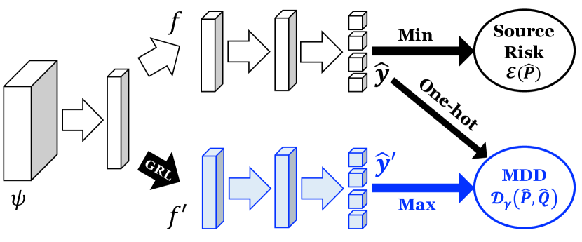
Figure 1: The adversarial network for algorithm implementation.

Now we design an adversarial learning algorithm to solve this problem by introducing an auxiliary classifier $f^{\prime}$ sharing the same hypothesis space with $f$. This is natively implemented in an adversarial network as Figure 1. Also since the margin loss is hard to optimize via stochastic gradient descent (SGD) in practice, we use a combination of loss functions $L$ and $L^{\prime}$ in substitution to the margin loss, which well preserve the key property of the margin. The practical optimization problem in the adversarial learning is stated as

$$\begin{gathered}\min_{f,\psi}\;\mathcal{E}(\widehat{P})+\eta\mathcal{D}_{\gamma}(\widehat{P},\widehat{Q}),\\ \max_{f^{\prime}}\;\mathcal{D}_{\gamma}(\widehat{P},\widehat{Q}),\end{gathered}$$ (25)

where $\eta$ is the trade-off coefficient between source error $\mathcal{E}(\widehat{P})$ and MDD $\mathcal{D}_{\gamma}(\widehat{P},\widehat{Q})$, $\gamma\triangleq\exp\rho$ is designed to attain the margin $\rho$ (detailed in the next subsection). Concretely,

$$\mathcal{E}(\widehat{P}) =\mathds{E}_{(x^{s},y^{s})\sim\widehat{P}}\,L(f(\psi(x^{s})),y^{s}),$$ (26)

$$\mathcal{D}_{\gamma}(\widehat{P},\widehat{Q}) =\mathds{E}_{x^{t}\sim\widehat{Q}}L^{\prime}(f^{\prime}(\psi(x^{t})),f(\psi(x^{t})))$$

$$-\gamma\mathds{E}_{x^{s}\sim\widehat{P}}L(f^{\prime}(\psi(x^{s})),f(\psi(x^{s}))).$$

Since the discrepancy loss term is not differentiable on the parameters of $f$, for simplicity we directly train the feature extractor $\psi$ to minimize the discrepancy loss term through a gradient reversal layer (GRL) (Ganin & Lempitsky, 2015).

4.2 Combined Cross-Entropy Loss

As we mentioned above, multiclass margin loss or hinge loss causes the problem of gradient vanishing in stochastic gradient descent, and thus cannot be optimized efficiently, especially for representation learning that significantly relies on gradient propagation. To overcome this common issue, we choose different loss functions on source and target and reweigh them to approximate MDD.

Denote by $\sigma$ the softmax function, i.e., for $\mathbf{z}\in\mathds{R}^{k}$

$$\sigma_{j}(\mathbf{z})={\frac{e^{z_{j}}}{\sum_{i=1}^{k}e^{z_{i}}}},\;\mathrm{for}\ j=1,\ldots,k.$$ (27)

On the source domain, $\mathrm{err}_{\widehat{P}}^{(\rho)}(f)$ and $\mathrm{disp}_{\widehat{P}}^{(\rho)}(f^{\prime},f)$ are replaced by the standard cross-entropy loss

$$L(f(\psi(x^{s})),y^{s}) \triangleq-\log[\sigma_{y^{s}}(f(\psi(x^{s})))],$$ (28)

$$L(f^{\prime}(\psi(x^{s})),f(\psi(x^{s}))) \triangleq-\log[\sigma_{h_{f}(\psi(x^{s}))}(f^{\prime}(\psi(x^{s})))].$$

On the target domain, we use a modified cross-entropy loss

$$L^{\prime}(f^{\prime}(\psi(x^{t})),\!f(\psi(x^{t})))\triangleq\log[1-\sigma_{h_{f}(\psi(x^{t}))}(f^{\prime}(\psi(x^{t}\!)))].$$ (29)

Note that this modification was introduced in Goodfellow et al. (2014) to mitigate the burden of exploding or vanishing gradients when performing adversarial learning. Combining the above two terms with a coefficient $\gamma$, the objective of the auxiliary classifier $f^{\prime}$ can be formulated as

$$\max_{f^{\prime}}\;\gamma \mathds{E}_{x^{s}\sim\widehat{P}}\log[\sigma_{h_{f}(\psi(x^{s}))}(f^{\prime}(\psi(x^{s})))]$$ (30)

$$+ \mathds{E}_{x^{t}\sim\widehat{Q}}\log[1-\sigma_{h_{f}(\psi(x^{t}))}(f^{\prime}(\psi(x^{t})))].$$

We shall see that training the feature extractor $\psi$ to minimize loss function (30) will lead to $\psi(\widehat{P})\approx\psi(\widehat{Q})$.

Proposition 4.1.

(Informal) Assuming that there is no restriction on the choice of $f^{\prime}$ and $\gamma>1$, the global minimum of the loss function (30) is $P=Q$. The value of $\sigma_{h_{f}}(f^{\prime}(\cdot))$ at equilibrium is ${\gamma}/{(1+\gamma)}$ and the corresponding margin of $f^{\prime}$ is $\log\gamma$.

We refer to $\gamma=\exp\rho$ as the margin factor, with explanation given in the Appendix (Theorems D.1 & D.2). In general larger $\gamma$ yields better generalization. However, as we have explained in Section 3, we cannot let it go to infinity. In fact, from an empirical view $\rho$ can only be chosen far beyond the theoretical optimal value since performing SGD for a large $\gamma$ might lead to exploding gradients. In summary, the choice of $\gamma$ is crucial in our method and we prefer relatively larger $\gamma$ in practice when exploding gradients are not encountered.

Table 1: Accuracy (%) on Office-31 for unsupervised domain adaptation (ResNet-50).

Method	A $\rightarrow$ W	D $\rightarrow$ W	W $\rightarrow$ D	A $\rightarrow$ D	D $\rightarrow$ A	W $\rightarrow$ A	Avg
ResNet-50 (He et al., 2016)	68.4$\pm$0.2	96.7$\pm$0.1	99.3$\pm$0.1	68.9$\pm$0.2	62.5$\pm$0.3	60.7$\pm$0.3	76.1
DAN (Long et al., 2015)	80.5$\pm$0.4	97.1$\pm$0.2	99.6$\pm$0.1	78.6$\pm$0.2	63.6$\pm$0.3	62.8$\pm$0.2	80.4
DANN (Ganin et al., 2016)	82.0$\pm$0.4	96.9$\pm$0.2	99.1$\pm$0.1	79.7$\pm$0.4	68.2$\pm$0.4	67.4$\pm$0.5	82.2
ADDA (Tzeng et al., 2017)	86.2$\pm$0.5	96.2$\pm$0.3	98.4$\pm$0.3	77.8$\pm$0.3	69.5$\pm$0.4	68.9$\pm$0.5	82.9
JAN (Long et al., 2017)	85.4$\pm$0.3	97.4$\pm$0.2	99.8$\pm$0.2	84.7$\pm$0.3	68.6$\pm$0.3	70.0$\pm$0.4	84.3
GTA (Sankaranarayanan et al., 2018)	89.5$\pm$0.5	97.9$\pm$0.3	99.8$\pm$0.4	87.7$\pm$0.5	72.8$\pm$0.3	71.4$\pm$0.4	86.5
MCD (Saito et al., 2018)	88.6$\pm$0.2	98.5$\pm$0.1	100.0$\pm$.0	92.2$\pm$0.2	69.5$\pm$0.1	69.7$\pm$0.3	86.5
CDAN (Long et al., 2018)	94.1$\pm$0.1	98.6$\pm$0.1	100.0$\pm$.0	92.9$\pm$0.2	71.0$\pm$0.3	69.3$\pm$0.3	87.7
MDD (Proposed)	94.5$\pm$0.3	98.4$\pm$0.1	100.0$\pm$.0	93.5$\pm$0.2	74.6$\pm$0.3	72.2$\pm$0.1	88.9

Table 2: Accuracy (%) on Office-Home for unsupervised domain adaptation (ResNet-50).

Method	Ar$\shortrightarrow$Cl	Ar$\shortrightarrow$Pr	Ar$\shortrightarrow$Rw	Cl$\shortrightarrow$Ar	Cl$\shortrightarrow$Pr	Cl$\shortrightarrow$Rw	Pr$\shortrightarrow$Ar	Pr$\shortrightarrow$Cl	Pr$\shortrightarrow$Rw	Rw$\shortrightarrow$Ar	Rw$\shortrightarrow$Cl	Rw$\shortrightarrow$Pr	Avg
ResNet-50 (He et al., 2016)	34.9	50.0	58.0	37.4	41.9	46.2	38.5	31.2	60.4	53.9	41.2	59.9	46.1
DAN (Long et al., 2015)	43.6	57.0	67.9	45.8	56.5	60.4	44.0	43.6	67.7	63.1	51.5	74.3	56.3
DANN (Ganin et al., 2016)	45.6	59.3	70.1	47.0	58.5	60.9	46.1	43.7	68.5	63.2	51.8	76.8	57.6
JAN (Long et al., 2017)	45.9	61.2	68.9	50.4	59.7	61.0	45.8	43.4	70.3	63.9	52.4	76.8	58.3
CDAN (Long et al., 2018)	50.7	70.6	76.0	57.6	70.0	70.0	57.4	50.9	77.3	70.9	56.7	81.6	65.8
MDD (Proposed)	54.9	73.7	77.8	60.0	71.4	71.8	61.2	53.6	78.1	72.5	60.2	82.3	68.1

5 Experiments

We evaluate the proposed learning method on three datasets against state of the art deep domain adaptation methods. The code is available at github.com/thuml/MDD.

5.1 Setup

Office-31 (Saenko et al., 2010) is a standard domain adaptation dataset of three diverse domains, Amazon from Amazon website, Webcam by web camera and DSLR by digital SLR camera with 4,652 images in 31 unbalanced classes.

Office-Home (Venkateswara et al., 2017) is a more complex dataset containing 15,500 images from four visually very different domains: Artistic images, Clip Art, Product images, and Real-world images.

VisDA-2017 (Peng et al., 2017) is simulation-to-real dataset with two extremely distinct domains: Synthetic renderings of 3D models and Real collected from photo-realistic or real-image datasets. With 280K images in 12 classes, the scale of VisDA-2017 brings challenges to domain adaptation.

We compare our designed algorithm based on Margin Disparity Discrepancy (MDD) with state of the art domain adaptation methods: Deep Adaptation Network (DAN) (Long et al., 2015), Domain Adversarial Neural Network (DANN) (Ganin et al., 2016), Joint Adaptation Network (JAN) (Long et al., 2017), Adversarial Discriminative Domain Adaptation (ADDA) (Tzeng et al., 2017), Generate to Adapt (GTA) (Sankaranarayanan et al., 2018), Maximum Classifier Discrepancy (MCD) (Saito et al., 2018), and Conditional Domain Adversarial Network (CDAN) (Long et al., 2018).

We follow the commonly used experimental protocol for unsupervised domain adaptation from Ganin & Lempitsky (2015); Long et al. (2018). We report the average accuracies of five independent experiments. The importance-weighted cross-validation (IWCV) is employed in all experiments for the selection of hyper-parameters. The asymptotic value of coefficient $\eta$ is fixed to $0.1$ and $\gamma$ is chosen from $\{2,3,4\}$ and kept the same for all tasks on the same dataset.

We implement our algorithm in PyTorch. ResNet-50 (He et al., 2016) is adopted as the feature extractor with parameters fine-tuned from the model pre-trained on ImageNet (Russakovsky et al., 2014). The main classifier and auxiliary classifier are both 2-layer neural networks with width 1024. For optimization, we use the mini-batch SGD with the Nesterov momentum 0.9. The learning rate of the classifiers are set 10 times to that of the feature extractor, the value of which is adjusted according to Ganin et al. (2016).

Table 3: Accuracy (%) on VisDA-2017 (ResNet-50).

Method	Synthetic $\rightarrow$ Real
JAN (Long et al., 2017)	61.6
MCD (Saito et al., 2018)	69.2
GTA (Sankaranarayanan et al., 2018)	69.5
CDAN (Long et al., 2018)	70.0
MDD (Proposed)	74.6

5.2 Results

The results on Office-31 are reported in Table 1. MDD achieves state of the art accuracies on five out of six transfer tasks. Notice that in previous works, feature alignment methods (JAN, CDAN) generally perform better for large-to-small tasks (A$\to$W, A$\to$D) while pixel-level adaptation methods (GTA) tend to obtain higher accuracy for small-to-large ones (W$\to$A, D$\to$A). Nevertheless our algorithm outperforms both types of methods on almost all task, showing its efficacy and universality. Tables 2 and 3 present the accuracies of our algorithm on Office-Home and VisDA-2017, where we make remarkable performance boost. Some of the methods listed in the tables use additional techniques such as the entropy minimization to enhance their performance. Our method possesses both simplicity and performance strength.

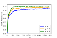
(a) Test Accuracy

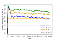
(b) Equilibrium on Source

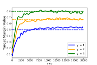
(c) Equilibrium on Target

Figure 2: Test accuracy and empirical values of $\sigma_{h_{f}}\mathop{\scalebox{0.6}{$\circ$}}f^{\prime}$ on transfer task D $\rightarrow$ A, where dashed lines indicate $\gamma/(1+\gamma)$.

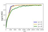
(a) MDD w/o Minimization

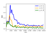
(b) DD

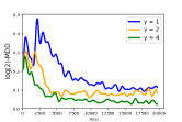
(c) $\log 2$-MDD

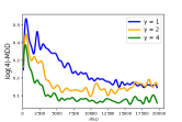
(d) $\log 4$-MDD

Figure 3: Empirical values of the margin disparity discrepancy (MDD) computed by auxiliary classifier $f^{\prime}$.

5.3 Analyses

In our adversarial learning algorithm, we reasonably use the combined cross-entropy loss instead of the margin loss and margin disparity discrepancy in our theory. We need to show that despite the technical modification, our algorithm can well reduce empirical MDD computed according to $f^{\prime}$:

$$\mathrm{disp}_{\widehat{Q}}^{(\rho)}(f^{\prime},f)-\mathrm{disp}_{\widehat{P}}^{(\rho)}(f^{\prime},f).$$ (31)

We choose $\gamma=1,2,4$ for comparison. The expected margin should reach $\log 2$ and $\log 4$ in the last two cases while there is no guarantee for margin with $\gamma=1$. Correspondingly, we examine DD (based on 0-1 loss), $\log 2$-MDD and $\log 4$-MDD for task D$\to$A and show results in Figures 2–3.

Table 4: Accuracy (%) on Office-31 by different margins.

Margin $\gamma$	A $\rightarrow$ W	D $\rightarrow$ A	Avg on Office-31
1	92.5	72.4	87.6
2	93.7	73.0	88.1
3	94.0	73.7	88.5
4	94.5	74.6	88.9
5	93.8	74.3	88.7
6	93.5	74.2	88.6

First, we justify that without the minimization part of the adversarial training, the auxiliary classifier $f^{\prime}$ in Eq. (30) is close to the $f^{\prime}$ that maximizes MDD over $\mathcal{F}$. We solve this optimization problem by directly training with the auxiliary classifier and show our results in 3(a), where MDD reaches $1$ shortly after training begins, implying that the loss function we use can well substitute MDD.

Next, we consider the equilibrium of the minimax optimization. The average values of $\sigma_{h_{f}}\mathop{\scalebox{0.6}{$\circ$}}f^{\prime}$ are presented in Figures 2(b) and 2(c). We could see that at the final training stage, $\sigma_{h_{f}}\mathop{\scalebox{0.6}{$\circ$}}f^{\prime}$ is close to the predicted value $\gamma/(1+\gamma)$ on the target (Section 4.1), which gives rise to large margin.

Last, by visualizing the values of DD, $\log 2$-MDD and $\log 4$-MDD and test accuracy computed over the whole dataset every 100 steps, we could see that relatively larger $\gamma$ leads to smaller MDD and higher test accuracy. Despite difficulties in gradient saturation, results using the original MDD loss are also comparable as shown in Appendix (See Table E.1).

6 Related Work

Domain Adaptation Theory.

One of the pioneering theoretical works in this field was conducted by Ben-David et al. (2007). They proposed the $\mathcal{H}\Delta\mathcal{H}$-divergence as a substitution of traditional distribution discrepancies (e.g. total variation, KL-divergence), which overcame the difficulties in estimation from finite samples. Mansour et al. (2009c) considered a general class of loss functions satisfying symmetry and subadditivity and developed a generalization theory with respect to the newly proposed discrepancy distance. The concurrent work in this setting was made by Kuroki et al. (2019), who introduced a tractable and finer counterpart for $\mathcal{H}\Delta\mathcal{H}$-divergence called S-disc computed with the ideal source classifier and similar class of loss functions with (Mansour et al., 2009c). In fact this measurement is encompassed in our DD as a special case. Mohri & Medina (2012); Zhang et al. (2012) proposed $\mathcal{Y}$-disc for domain adaptation with partially labeled target data. Cortes & Mohri (2014); Cortes et al. (2015) further proposed a theory for regression tasks in the setting of domain adaptation via the generalized discrepancy. Another line of theoretical works on domain adaptation puts emphasis on the assumptions of the different distributions. Zhang et al. (2013); Gong et al. (2016) tackled this problem from a causal view and put forward the generalized target shift (GeTarS) scenario instead of the traditional assumption of covariate shift. Germain et al. (2013) proposed a PAC-Bayesian theory for domain adaptation using the domain disagreement pseudometric.

Domain Adaptation Algorithm.

Domain adaptation methods based on deep networks have achieved great success in recent years (Long et al., 2015; Ganin & Lempitsky, 2015). These works aim to learn domain-invariant representations by minimizing a certain discrepancy between distributions of source and target features extracted by a shared representation learner. With insights from both the theory of Ben-David et al. (2010) and the practice of adversarial learning (Goodfellow et al., 2014), Ganin & Lempitsky (2015) put forward the domain adversarial neural network (DANN). A domain discriminator is trained to distinguish source features from target features and a feature extractor to confuse the discriminator. Since then, a series of works have appeared and achieved significantly better performance. Tzeng et al. (2017) proposed an architecture that employed asymmetric encodings for target and source data. Long et al. (2018) presented a principled framework that conducted the adversarial adaptation models using conditional information. Hoffman et al. (2018b); Sankaranarayanan et al. (2018) unified pixel-level and feature-level adversarial learning for domain adaptation. Saito et al. (2018) considered the classifiers instead of features and designed an original adversarial learning method by maximizing the classifier discrepancy.

7 Conclusion

In this paper, we derived novel generalization bounds based on newly proposed margin disparity discrepancy, and presented both theoretical and algorithmic analyses of domain adaptation. Our analyses are more general for analyzing real-world domain adaptation problems, and the well-designed theory-induced algorithm achieves the state of the art results.

References

- Anthony & Bartlett (2009) Anthony, M. and Bartlett, P. L. Neural network learning: Theoretical foundations. cambridge university press, 2009.
- Ben-David et al. (2007) Ben-David, S., Blitzer, J., Crammer, K., and Pereira, F. Analysis of representations for domain adaptation. In Advances in Neural Information Processing Systems (NeurIPS), 2007.
- Ben-David et al. (2010) Ben-David, S., Blitzer, J., Crammer, K., Kulesza, A., Pereira, F., and Vaughan, J. W. A theory of learning from different domains. Machine Learning, 79(1-2):151–175, 2010.
- Blitzer et al. (2008) Blitzer, J., Crammer, K., Kulesza, A., Pereira, F., and Wortman, J. Learning bounds for domain adaptation. In Advances in Neural Information Processing Systems (NeurIPS), pp. 129–136. 2008.
- Cortes & Mohri (2014) Cortes, C. and Mohri, M. Domain adaptation and sample bias correction theory and algorithm for regression. Theoretical Computer Science, 519:103–126, 2014.
- Cortes et al. (2015) Cortes, C., Mohri, M., and Muñoz Medina, A. Adaptation algorithm and theory based on generalized discrepancy. In ACM SIGKDD International Conference on Knowledge Discovery and Data Mining (KDD), pp. 169–178, 2015.
- Courty et al. (2017) Courty, N., Flamary, R., Habrard, A., and Rakotomamonjy, A. Joint distribution optimal transportation for domain adaptation. In Advances in Neural Information Processing Systems (NeurIPS), pp. 3730–3739. 2017.
- Crammer et al. (2008) Crammer, K., Kearns, M., and Wortman, J. Learning from multiple sources. Journal of Machine Learning Research (JMLR), 9:1757–1774, 2008.
- Ganin & Lempitsky (2015) Ganin, Y. and Lempitsky, V. Unsupervised domain adaptation by backpropagation. In International Conference on Machine Learning (ICML), 2015.
- Ganin et al. (2016) Ganin, Y., Ustinova, E., Ajakan, H., Germain, P., Larochelle, H., Laviolette, F., Marchand, M., and Lempitsky, V. Domain-adversarial training of neural networks. Journal of Machine Learning Research (JMLR), 17:2096–2030, 2016.
- Germain et al. (2013) Germain, P., Habrard, A., Laviolette, F., and Morvant, E. A pac-bayesian approach for domain adaptation with specialization to linear classifiers. In International Conference on Machine Learning (ICML), pp. 738–746, 2013.
- Gong et al. (2016) Gong, M., Zhang, K., Liu, T., Tao, D., Glymour, C., and Schölkopf, B. Domain adaptation with conditional transferable components. In International conference on machine learning (ICML), pp. 2839–2848, 2016.
- Goodfellow et al. (2014) Goodfellow, I., Pouget-Abadie, J., Mirza, M., Xu, B., Warde-Farley, D., Ozair, S., Courville, A., and Bengio, Y. Generative adversarial nets. In Advances in Neural Information Processing Systems (NeurIPS), 2014.
- Gretton et al. (2012) Gretton, A., Borgwardt, K., Rasch, M., Schölkopf, B., and Smola, A. A kernel two-sample test. Journal of Machine Learning Research (JMLR), 13:723–773, 2012.
- He et al. (2016) He, K., Zhang, X., Ren, S., and Sun, J. Deep residual learning for image recognition. In IEEE Conference on Computer Vision and Pattern Recognition (CVPR), 2016.
- Hoffman et al. (2018a) Hoffman, J., Mohri, M., and Zhang, N. Algorithms and theory for multiple-source adaptation. In Advances in Neural Information Processing Systems (NeurIPS), pp. 8256–8266. 2018a.
- Hoffman et al. (2018b) Hoffman, J., Tzeng, E., Park, T., Zhu, J.-Y., Isola, P., Saenko, K., Efros, A., and Darrell, T. CyCADA: Cycle-consistent adversarial domain adaptation. In International Conference on Machine Learning (ICML), pp. 1989–1998, 2018b.
- Koltchinskii et al. (2002) Koltchinskii, V., Panchenko, D., et al. Empirical margin distributions and bounding the generalization error of combined classifiers. The Annals of Statistics, 30(1):1–50, 2002.
- Kuroki et al. (2019) Kuroki, S., Charonenphakdee, N., Bao, H., Honda, J., Sato, I., and Sugiyama, M. Unsupervised domain adaptation based on source-guided discrepancy. In AAAI Conference on Artificial Intelligence (AAAI), 2019.
- Long et al. (2015) Long, M., Cao, Y., Wang, J., and Jordan, M. I. Learning transferable features with deep adaptation networks. In International Conference on Machine Learning (ICML), 2015.
- Long et al. (2017) Long, M., Wang, J., and Jordan, M. I. Deep transfer learning with joint adaptation networks. In International Conference on Machine Learning (ICML), 2017.
- Long et al. (2018) Long, M., Cao, Z., Wang, J., and Jordan, M. I. Conditional adversarial domain adaptation. In Advances in Neural Information Processing Systems (NeurIPS), pp. 1647–1657. 2018.
- Mansour et al. (2009a) Mansour, Y., Mohri, M., and Rostamizadeh, A. Multiple source adaptation and the rényi divergence. In Conference on Uncertainty in Artificial Intelligence, pp. 367–374. AUAI Press, 2009a.
- Mansour et al. (2009b) Mansour, Y., Mohri, M., and Rostamizadeh, A. Domain adaptation with multiple sources. In Advances in Neural Information Processing Systems (NeurIPS), pp. 1041–1048. 2009b.
- Mansour et al. (2009c) Mansour, Y., Mohri, M., and Rostamizadeh, A. Domain adaptation: Learning bounds and algorithms. In Conference on Learning Theory (COLT), 2009c.
- Mendelson & Vershynin (2003) Mendelson, S. and Vershynin, R. Entropy and the combinatorial dimension. Inventiones mathematicae, 152(1):37–55, 2003.
- Mohri & Medina (2012) Mohri, M. and Medina, A. M. New analysis and algorithm for learning with drifting distributions. In International Conference on Algorithmic Learning Theory, pp. 124–138, 2012.
- Mohri et al. (2012) Mohri, M., Rostamizadeh, A., and Talwalkar, A. Foundations of machine learning. 2012.
- Pan & Yang (2010) Pan, S. J. and Yang, Q. A survey on transfer learning. IEEE Transactions on Knowledge and Data Engineering (TKDE), 22(10):1345–1359, 2010.
- Pan et al. (2011) Pan, S. J., Tsang, I. W., Kwok, J. T., and Yang, Q. Domain adaptation via transfer component analysis. IEEE Transactions on Neural Networks (TNN), 22(2):199–210, 2011.
- Peng et al. (2017) Peng, X., Usman, B., Kaushik, N., Hoffman, J., Wang, D., and Saenko, K. Visda: The visual domain adaptation challenge. CoRR, abs/1710.06924, 2017.
- Quionero-Candela et al. (2009) Quionero-Candela, J., Sugiyama, M., Schwaighofer, A., and Lawrence, N. D. Dataset shift in machine learning. The MIT Press, 2009.
- Rakhlin & Sridharan (2014) Rakhlin, A. and Sridharan, K. Statistical learning and sequential prediction. Book Draft, 2014.
- Russakovsky et al. (2014) Russakovsky, O., Deng, J., Su, H., Krause, J., Satheesh, S., Ma, S., Huang, Z., Karpathy, A., Khosla, A., Bernstein, M., Berg, A. C., and Fei-Fei, L. ImageNet Large Scale Visual Recognition Challenge. 2014.
- Saenko et al. (2010) Saenko, K., Kulis, B., Fritz, M., and Darrell, T. Adapting visual category models to new domains. In European Conference on Computer Vision (ECCV), 2010.
- Saito et al. (2018) Saito, K., Watanabe, K., Ushiku, Y., and Harada, T. Maximum classifier discrepancy for unsupervised domain adaptation. In IEEE Conference on Computer Vision and Pattern Recognition (CVPR), pp. 3723–3732, 2018.
- Sankaranarayanan et al. (2018) Sankaranarayanan, S., Balaji, Y., Castillo, C. D., and Chellappa, R. Generate to adapt: Aligning domains using generative adversarial networks. In IEEE Conference on Computer Vision and Pattern Recognition (CVPR), 2018.
- Talagrand (2014) Talagrand, M. Upper and lower bounds for stochastic processes: modern methods and classical problems, volume 60. Springer Science & Business Media, 2014.
- Tzeng et al. (2014) Tzeng, E., Hoffman, J., Zhang, N., Saenko, K., and Darrell, T. Deep domain confusion: Maximizing for domain invariance. CoRR, abs/1412.3474, 2014.
- Tzeng et al. (2017) Tzeng, E., Hoffman, J., Saenko, K., and Darrell, T. Adversarial discriminative domain adaptation. In IEEE Conference on Computer Vision and Pattern Recognition (CVPR), 2017.
- Venkateswara et al. (2017) Venkateswara, H., Eusebio, J., Chakraborty, S., and Panchanathan, S. Deep hashing network for unsupervised domain adaptation. In IEEE Conference on Computer Vision and Pattern Recognition (CVPR), 2017.
- Zhang et al. (2012) Zhang, C., Zhang, L., and Ye, J. Generalization bounds for domain adaptation. In Advances in Neural Information Processing Systems (NeurIPS), pp. 3320–3328. 2012.
- Zhang et al. (2013) Zhang, K., Schölkopf, B., Muandet, K., and Wang, Z. Domain adaptation under target and conditional shift. In International Conference on Machine Learning (ICML), pp. 819–827, 2013.
- Zhou (2002) Zhou, D.-X. The covering number in learning theory. Journal of Complexity, 18(3):739–767, 2002.