Evolution of intensive light pulses in a nonlinear medium with the Raman effect

Аннотация

In this paper, we study the evolution of intensive light pulses in nonlinear single-mode fibers. The dynamics of light in such fibers is described by the nonlinear Schrödinger equation with the Raman term, due to stimulated Raman self-scattering. It is shown that dispersive shock waves are formed during the evolution of sufficiently intensive pulses. In this case the situation is much richer than for the nonlinear Schrödinger equation with Kerr nonlinearity only. The Whitham equations are obtained under the assumption that the Raman term can be considered as a small perturbation. These equations describe slow evolution of dispersive shock waves. It is shown that if one takes into account the Raman effect, then dispersive shock waves can asymptotically acquire a stationary profile. The analytical theory is confirmed by numerical calculations.

Keywords: nonlinear medium, Raman effect, dispersive shock waves, solitons, Whitham modulation equations.

1 Introduction

The problem of evolution of light pulses in wave-guides is a subject of active modern experimental and theoretical research. It is well known that if one neglects the effects of dissipation and dispersion, then the theory of nonlinear propagation of light envelope suffers from a wave breaking singularity developed at some finite fiber length after which a formal solution of nonlinear wave equations becomes multi-valued and loses its physical meaning. The account of dispersion eliminates such a non-physical behavior, but the evolution equations for the envelopes acquire higher order derivatives which makes their analytical treatment more difficult. Nevertheless, the following qualitative picture of the phenomenon can be inferred from numerical experiments. After the wave breaking moment, instead of multi-valued region, an expanding region of fast nonlinear oscillations is formed. Envelope parameters in such a structure change slowly compared with the characteristic oscillations frequency and their wavelength. This region of fast oscillations is called ‘‘dispersive shock wave’’ (DSW). In nonlinear optics, such structures were observed long ago (see, for instance, tsj-85 ; rg-89 ). But even earlier this phenomenon had been studied in the water waves dynamics (see, for instance, BenLigh-1954 ) and plasma physics (see, for instance, tbi-70 ). The general nature of this phenomenon, which arises as a result of interplay of nonlinear and dispersion effects with low viscosity, was studied by R. Z. Sagdeev Sagdeev-1964 . The introduction of small dissipation can, in some cases, balance the dispersive effects so that the DSW eventually acquires a steady profile, but remains oscillatory in space. The simplest and, apparently, most powerful theoretical approach to a description of DSWs was formulated by Gurevich and Pitaevskii GP-1973 in framework of the Whitham theory of modulation of nonlinear waves whitham-65 ; whitham-77 which was based on large difference between scales of the wavelength of nonlinear oscillations within DSW and the size of the whole DSW. To date, the theory and experimental investigations of DSWs have been greatly developed, It has spread to other fields of nonlinear physics, including the dynamics of nonlinear waves in a Bose-Einstein condensates; see, for instance, the review article ElHoefer-2016 and references therein. In particular, the theory of DSWs has been applied to the nonlinear Schrödinger (NLS) equation for media with normal dispersion and Kerr nonlinearity gk-87 ; eggk-95 . And it agrees perfectly well with experimental studies of the evolution of specially formed rectangular pulses in optical fibers Xu-2017 .

The NLS equation theory is one of the main ways of describing waves in nonlinear optics and it usually gives a good qualitative explanation of the main features of the phenomenon. However, it often turns out to be insufficient for quantitative interpretation of the emerging DSWs. Sometimes even small corrections to the NLS equation, caused by taking into account small additional effects, lead to a sufficiently radical deviations for long evolution from predictions of the NLS equation theory. As was demonstrated in Zakh-1971 , the NLS equation belongs to a special class of so-called completely integrable equations. Going beyond this class makes the inverse scattering method used in the theory of the NLS equation inapplicable. For instance, optical shock waves were observed in intensive light beams propagating in photorefractive crystals with defocusing saturated nonlinearity wjf-2007 , so by increasing the intensity of the wave, the relative role of nonlinearity decreases, which is not considered in the NLS theory. In this case, the Whitham modulation equations are too complicated for finding their global analytical solution. In spite of that, for the special case of the initial condition in the form of an intensity step-like discontinuity, the method of the work El05 gives the main characteristics of DSW egkkk-07 . A similar theory can be developed for optical DSW in colloidal media ans-17 . A more general form of initial pulses can be considered with the use of the recently developed method Kamch-2019 .

Changing the type of nonlinearity can lead not only to quantitative differences from the NLS theory but also to qualitatively new effects. For instance, the delay of the nonlinear response of the medium to the wave field turns the NLS equation into so-called ‘‘derivative nonlinear Schrödinger equation’’, which contain in addition to the Kerr-type nonlinearity its time derivative. Such a modification of the NLS equation radically changes the theory of DSWs. As a result, new wave structures of the combined type become possible. For example, the oscillation region can be combined with rarefaction waves, as well as other wave configurations (see IvKamch-2017 ) can be observed.

Other qualitatively new effects are caused by small perturbations of dissipative type. These perturbations at a sufficiently large time become comparable with small modulation of the wave packet, which can lead to the stabilization of DSW so that it acquires a stationary profile. This phenomenon can also occur when one takes into account the Raman effect in the propagation of light pulses in the wave-guides. As was mentioned in Kivshar-1990 , in the small-amplitude approximation, the NLS equation with an additional Raman term can be reduced to the Korteweg-de Vries-Burgers (KdV-B) equation. The presence of stationary DSWs for the KdV-B equation was established in johnson-70 by the direct perturbation theory (gp-87 ; akn-87 ) and by using the Whitham method (see also Kamchatnov-2016 ). However, taking into account perturbing terms of this type in the NLS theory is much more complicated (Kamch-2004 ; lpk-12 ) and therefore requires separate consideration. The aim of this work is to study the impact of the Raman effect, which is caused by the influence of retardation of the fiber material response to variations of the electromagnetic signal on the dynamics of light pulses propagating in a single-mode fiber. First, in section 3, we consider the influence of this effect on the dynamics of linear waves that propagate along a uniform background. In section 4 we find the leading dispersion and nonlinear corrections to the dispersionless linear propagation of disturbances since some qualitative features of the behavior of a light pulse envelope in fiber can be already explained by the small-amplitude limit of the evolution equations. Then we proceed to the description of several stages in the DSW evolution after wave breaking. As will be shown, in the first stage, when the length of light propagation through the fiber is sufficiently small, the Raman effect can be neglected. Then the system can be described by the ordinary NLS equation with Kerr nonlinearity. The solution of the Whitham equations for this equation in some characteristic cases is well known. At the next stage, the Raman effect becomes efficient. In this case, the evolution of the DSW is described by the perturbed Whitham equations, which will be derived in section 5 within the framework of the theory developed in Kamch-2004 . We will show that this effect affects differently on the waves that propagate in different directions. Finally, it will be shown that the shock wave directed in the positive direction of the time axis $t$ becomes stationary, while the parameters of the DSW propagating in the opposite direction continue to evolve with increasing amplitude of the DSW and the duration of the wave structure. The analytical results obtained in the work are confirmed by numerical calculations.

2 The model

We proceed from a standard approach (see, for instance, KivsharAgrawal-2003 ), in which the dynamics of the electric field envelope $E(x,t)$ of the light wave is described by the NLS equation taking into account normal dispersion and defocusing Kerr nonlinearity, whereas we neglect attenuation:

$$\frac{\partial E}{\partial X}+\beta_{1}\frac{\partial E}{\partial T}+\frac{i}{2}\beta_{2}\frac{\partial^{2}E}{\partial T^{2}}-i\tilde{\gamma}|E|^{2}E=0,$$ (1)

where $X$ is a coordinate along the waveguide, $T$ is a time, $\beta_{1}$ is reverse group velocity of the waves ($v_{gr}=1/\beta_{1}$) and $\beta_{2}$ is the parameter that determines pulse expansion, $\tilde{\gamma}$ is non-linear coefficient which determined by the expression

$$\tilde{\gamma}=\frac{n_{2}\omega_{0}}{c_{l}E_{eff}},\qquad E_{eff}=\pi w^{2}$$

for the carrier frequency $\omega_{0}$. Here $w$ is the parameter of the Gaussian mode, $n_{2}$ is the nonlinear refractive index, $c_{l}$ is the light velocity in vacuum. Thus, the second term in the evolution equation (1) describes wave transfer with group velocity, and the last term corresponds to Kerr nonlinearity. The term with the positive coefficient $\beta_{2}>0$ is a quadratic dispersion. Equation (1) by substitution

$$x=-\tilde{\gamma}I_{0}X,\quad t=\sqrt{\frac{\tilde{\gamma}I_{0}}{\beta_{2}}}(T-\beta_{1}X),\quad q=\frac{E}{\sqrt{I_{0}}},$$

where $I_{0}$ is the characteristic intensity of the system, is converted to a conventional dimensionless form

$$iq_{x}+\frac{1}{2}q_{tt}-|q|^{2}q=0.$$ (2)

As mentioned in the Introduction, the propagation of pulses along sufficiently long fibers is significantly affected by small effects that are not taken into account in the NLS approximation, such as higher-order dispersion, self-steepening and Raman scattering (Raman effect). The influence of the self-steepening effect on the DSW evolution was discussed in detail in IvKamch-2017 , where it was shown that it leads to the formation of complex combined structures. The Raman effect describes the mixing of the frequency of stimulated Raman self-scattering. And its consideration leads to an additional term in the evolution equation so that the equation for the light pulse envelope in dimensionless variables has a form

$$iq_{x}+\frac{1}{2}q_{tt}-|q|^{2}q+\gamma q(|q|^{2})_{t}=0.$$ (3)

Here $\gamma$ is a constant, which characterizes the slope of the SRS-gain line. It is usually a small parameter of the system, which allows us to consider the last term of the equation as a perturbation for the description of DSW in the Whitham theory. It is worth noting that the manifestations of the self-steepening and the Raman effect are quite different and therefore they can be identified separately.

We shall start with the study of linear waves which propagate along a uniform wave background.

3 Linear waves

Let the light pulse propagate along a uniform wave background with the amplitude $\sqrt{I_{0}}=|q_{0}|=\mathrm{const}$. To see the role of the Raman term, we find the solution of the linearized NLS equation with the Raman term for evolution of a pulse in a linear approximation. It is convenient to make a substitution $q(x,t)=\tilde{q}(x,t)\exp{(-{i}I_{0}x)}$. Then equation (3) takes the form

$$i\tilde{q}_{x}+\frac{1}{2}\tilde{q}_{tt}+(I_{0}-|\tilde{q}|^{2})\tilde{q}+\gamma\tilde{q}(|\tilde{q}|^{2})_{t}=0.$$ (4)

This replacement does not change the properties of the equation since the phase of the wave is determined up to a constant. The evolution of a small perturbation $\delta q$ propagating along a homogeneous background,

$$\tilde{q}=\sqrt{I_{0}}+\delta q,\qquad|\delta q|\ll\sqrt{I_{0}},$$ (5)

can be described by a linearized equation

$$i\delta q+\frac{1}{2}\delta q_{tt}-I_{0}(\delta q+\delta q^{*})+\gamma I_{0}(\delta q+\delta q^{*})_{t}=0$$ (6)

with the initial condition $\delta{q}|_{x=0}=\delta{q_{0}}(t)$. After separation of real and imaginary parts

$$\delta q=A+iB$$ (7)

we obtain from (6)

$$A_{x}+\frac{1}{2}B_{tt}=0,\quad B_{x}-\frac{1}{2}A_{tt}+2I_{0}A-2\gamma I_{0}A_{t}=0.$$ (8)

The function $B$ can be excluded, and then from this system we get a linear equation for $A$:

$$A_{xx}-I_{0}A_{tt}+\gamma I_{0}A_{ttt}+\frac{1}{4}A_{tttt}=0.$$ (9)

This equation can be solved by the Fourier method. To this end, we note that linear harmonic waves $A\propto\exp{[{i}(kx-\omega t)]}$ satisfy the dispersion law

$$k=\pm k(\omega),\quad k(\omega)=\omega\sqrt{\frac{\omega^{4}}{4}+I_{0}(1+i\gamma\omega)}.$$ (10)

The imaginary unit in the dispersion law means that for $\gamma\neq 0$ there is a damping or amplification of linear waves. General solution of the equation (9) can be written as

$$\begin{split}A(x,t)=&\int_{-\infty}^{+\infty}W_{1}(\omega)e^{i(k(\omega)x-\omega t)}\frac{d\omega}{2\pi}\\ &+\int_{-\infty}^{+\infty}W_{2}(\omega)e^{i(-k(\omega)x-\omega t)}\frac{d\omega}{2\pi},\end{split}$$ (11)

where functions $W_{1,2}(\omega)$ are determined from the initial conditions

$$\begin{split}A(0,t)&=\int_{-\infty}^{+\infty}[W_{1}(\omega)+W_{2}(\omega)]e^{-i\omega t}\frac{d\omega}{2\pi}\\ A_{x}(0,t)&=i\int_{-\infty}^{+\infty}k(\omega)[W_{1}(\omega)-W_{2}(\omega)]e^{-i\omega t}\frac{d\omega}{2\pi}.\end{split}$$ (12)

After standard calculations we arrive at the solution expressed in terms of the Fourier transform $\widehat{I^{\prime}_{0}}(\omega)$ and $\widehat{\varphi^{\prime}_{0}}(\omega)$ of the initial (input) intensity $I^{\prime}(x,t)=2\sqrt{I_{0}}A(x,t)$ and phase $\varphi^{\prime}(x,t)=B(x,t)/\sqrt{I_{0}}$ disturbances,

$$\begin{split}W_{1}(\omega)&=\frac{1}{4\sqrt{I_{0}}}\left[\widehat{I^{\prime}_{0}}(\omega)-i\frac{\omega^{2}}{k(\omega)}I_{0}\widehat{\varphi^{\prime}_{0}}(\omega)\right],\\ W_{1}(\omega)&=\frac{1}{4\sqrt{I_{0}}}\left[\widehat{I^{\prime}_{0}}(\omega)+i\frac{\omega^{2}}{k(\omega)}I_{0}\widehat{\varphi^{\prime}_{0}}(\omega)\right].\end{split}$$ (13)

Suppose that at the initial moment the phase of the wave is constant and there is only the intensity perturbation, that is, $\varphi^{\prime}_{0}=0$, then

$$\begin{split}I^{\prime}(t,x)=\frac{1}{4\pi}\int_{-\infty}^{+\infty}\widehat{I^{\prime}_{0}}(\omega)\left[e^{ixf_{1}(\omega)}+e^{ixf_{2}(\omega)}\right]d\omega,\end{split}$$ (14)

where

$$f_{1}(\omega)=k(\omega)-\omega\frac{t}{x},\quad f_{2}(\omega)=-k(\omega)-\omega\frac{t}{x}.$$ (15)

These integrals can be estimated for a large distance of propagation $x$ by the method of stationary phase resulting in

$$\delta I(t,x)\simeq\frac{2\widehat{I^{\prime}_{0}}(\omega^{(1)}_{0})}{\sqrt{2x{|\frac{d^{2}f_{1}}{d\omega^{2}}|}_{\omega_{0}^{(1)}}}}\cos{\left(xf_{1}(\omega^{(1)}_{0})-\frac{\pi}{4}\right)}$$ (16)

for the wave that propagates in the negative direction of the $t$-axis, and

$$\delta I(t,x)\simeq\frac{2\widehat{I^{\prime}_{0}}(\omega^{(2)}_{0})}{\sqrt{2x{|\frac{d^{2}f_{2}}{d\omega^{2}}|}_{\omega_{0}^{(2)}}}}\cos{\left(xf_{2}(\omega^{(2)}_{0})-\frac{\pi}{4}\right)}$$ (17)

for a linear wave propagating to the right. Here $\omega^{(1)}_{0}$ and $\omega^{(2)}_{0}$ are the values of $\omega$ at the points of the stationary phase that are defined by the equations

$$\frac{df_{1}}{d\omega}=0,\qquad\frac{df_{2}}{d\omega}=0.$$ (18)

Fig. 1: Evolution of the pulse in the linear approximation of the NLS equations with Raman term (3) with $\gamma=0.1$. The dashed gray line shows the initial perturbation, the dashed blue line corresponds to the stationary phase approximation (16) and (17), and the red solid line corresponds to the numerical calculation of the integral (14) for $x=4$ with the initial perturbation (19) with $a=1$. Black solid line shows linear waves obeying a linearized equation (6) with $\gamma=0$.

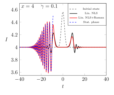
In figure 1 we compare the numerical calculations of the integral (14) with its approximate estimates (16) and (17) for the initial perturbation

$$I^{\prime}_{0}(t)=\frac{1}{\sqrt{\pi}a}\exp{\left(-\frac{t^{2}}{a^{2}}\right)},\quad\widehat{I^{\prime}_{0}}(\omega)=\exp{\left(-\frac{\omega^{2}a^{2}}{4}\right)}.$$ (19)

As we see, the pulse splits into two smaller pulses, however, on the contrary to the NLS case, they are not symmetrical pulses propagating in opposite directions. Now, these two pulses have different profiles. It can be seen that the pulse propagating in the positive direction of the $t$-axis attenuates, while the impulse propagates in the negative direction is amplified. This is the manifestation of lack of the time inversion invariance, which is caused by the last term in (3). The approximate solution (16), (17) shows that the amplitude of a linear wave packet propagating to the left increases monotonically. However, one should not forget that this theory is valid for small deviations from the background intensity. It should be noted that the asymptotic solution (16) and (17) describes well the wave packet even for not very large $x$.

Fig. 2: Evolution of the pulse in the linear approximation of the NLS equation with Raman term (3) with $\gamma=0.02$. The dashed gray line shows the initial perturbation as an initial discontinuity and the red solid line corresponds to the numerical calculation of the integral (14) for $x=5$ with the initial perturbation (20) with $I^{L}=0.5$, $I^{R}=0$ and $\Delta=0.3$. The black solid line shows the linear waves obeying the linearized equation (6) with $\gamma=0$.

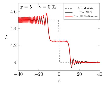
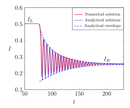
The figure 2 shows the dependence of linear wave intensity on time for the step-like initial condition, which we model by the formula

$$I^{\prime}_{0}(t)=\frac{1}{2}\left\{I^{R}+I^{L}+(I^{R}-I^{L})\tanh{\left(\frac{t}{\Delta}\right)}\right\},$$ (20)

where ‘‘step width’’ $\Delta$ should be taken small enough so that its effect disappears at sufficiently large time. The constants $I^{R}$ and $I^{L}$ are responsible for the boundary values of the light intensity on the right and left sides of discontinuity, respectively. The problem of the evolution of the initial discontinuity is one of the fundamental importance in the DSW theory, and we will consider it in detail below. Here we note that the difference between linear waves at $\gamma=0$ and at $\gamma\neq 0$ is noticeable even at small values of $\gamma$, especially for the left wave.

Let us turn now to the study of the effect of small dispersion and nonlinearity on the light pulse evolution.

4 Small-amplitude and weak dispersion limits

Let us turn to the study of the Raman effect influence on the evolution of a DSW in the small-amplitude and weak dispersion limit when they are taken into account in the main approximation. That is, we are interested in the leading dispersion and nonlinear corrections to the dispersionless linear propagation of disturbances along the uniform background $I_{0}$. To this end, it is convenient to use the physical variables of intensity $I(x,t)$ and chirp $u(x,t)$. To go to the equations for these variables, we apply the Madelung transform

$$q(x,t)=\sqrt{I(x,t)}\exp{\left({i}\int^{t}u(x,t^{\prime})dt^{\prime}\right)}.$$ (21)

After its substitution into Eq. (3), separation of the real and imaginary parts and differentiation of one of the equations with respect to $x$, we get the system

$$\begin{split}&I_{x}+(uI)_{t}=0,\\ &u_{x}+uu_{t}+I_{t}+\left(\frac{I^{2}_{t}}{8I^{2}}-\frac{I_{tt}}{4I}\right)_{t}=\gamma I_{tt}.\end{split}$$ (22)

The last term on the left-hand side of the second equation describes the dispersion, and the term on the right-hand side of this equation resembles the well-known Burgers viscosity in the theory of water waves and other continuous media whitham-77 .

Using the last system and applying the standard perturbation theory for the amplitude of the perturbation and for the weak dispersion (see, for example, kamch-2000 ), one can obtain a small-amplitude analog of the equation (3). Let the wave propagate in the positive direction of the $t$-axis. Then an approximate equation for $I^{\prime}=I-I_{0}$ takes the form

$$\begin{split}\frac{\partial I^{\prime}}{\partial x}+\sqrt{I_{0}}\frac{\partial I^{\prime}}{\partial t}&+\frac{3}{2\sqrt{I_{0}}}I^{\prime}\frac{\partial I^{\prime}}{\partial t}\\ &-\frac{1}{8\sqrt{I_{0}}}\frac{\partial^{3}I^{\prime}}{\partial t^{3}}=\frac{1}{2}\gamma\sqrt{I_{0}}\frac{\partial^{2}I^{\prime}}{\partial t^{2}}.\end{split}$$ (23)

This is the Korteweg-de Vries–Burgers equation (KdV–B). As is known (see gp-87 ; Kamchatnov-2016 ), the evolution of waves obeying this equation is divided into three stages. In the first stage, when $x\ll\gamma^{-1}$, the term that characterizes low viscosity has little effect on the evolution of DSW and therefore it is neglected. Then, in the second stage, when $x\sim\gamma^{-1}$, the influence of viscosity becomes comparable to the modulation of DSW. Obviously, in this case, viscosity cannot be neglected, and then perturbation theory is used to describe the DSW because of the smallness of the viscosity coefficient. Finally, at the third stage, at $x\gg\gamma^{-1}$, the DSW becomes stationary in $x$, that is the output signal profile ceases to depend on the fiber length. Such a behavior of the DSW should be expected in the case of the equation (3) for the wave propagating to the left.

However, the situation changes drastically for waves propagating in the opposite direction. For a perturbation of intensity $I^{\prime}$, the limiting equation is written in the form

$$\begin{split}\frac{\partial I^{\prime}}{\partial x}-\sqrt{I_{0}}\frac{\partial I^{\prime}}{\partial t}&+\frac{1}{\sqrt{I_{0}}}I^{\prime}\frac{\partial I^{\prime}}{\partial t}\\ &\frac{1}{8\sqrt{I_{0}}}\frac{\partial^{3}I^{\prime}}{\partial t^{3}}=-\frac{1}{2}\gamma\sqrt{I_{0}}\frac{\partial^{2}I^{\prime}}{\partial t^{2}}.\end{split}$$ (24)

This is also the KdV–B equation, but now it has opposite signs before the dispersion and viscosity. This means that the orientation of the DSW is changed, and wave amplification is expected instead of the standard attenuation of the wave.

This difference between the waves oppositely directed is caused by the absence of symmetry of the equation (3) with respect to the replacement $t\rightarrow-t$. Obviously, this property will affect the evolution of the pulse described by the complete equation (3). Let us turn to the description of the formation of DSWs and the derivation of equations describing their dynamics.

5 Dispersive shock wave formation

We first discuss the dispersionless limit of hydrodynamic equations that follows from the NLS equation (2) when the dispersion is neglected. In this limit, equations (22) without the Raman term is transferred to the system

$$\begin{split}&I_{x}+(uI)_{t}=0,\\ &u_{x}+uu_{t}+I_{t}=0,\end{split}$$ (25)

where the first equation can be interpreted as the continuity equation for the intensity $I$ and the second one as the Euler equation for the ‘‘flow velocity’’ $u$. This system can be cast in a standard way to the Riemann diagonal form

$$\frac{\partial r_{\pm}}{\partial x}+\frac{1}{v_{\pm}}\frac{\partial r_{\pm}}{\partial t}=0$$ (26)

for the Riemann invariants

$${r_{\pm}}=\frac{u}{2}\pm\sqrt{I}$$ (27)

with inverse velocities

$$\frac{1}{v_{\pm}}=u\pm\sqrt{I}.$$ (28)

The functions introduced here will be needed to select the initial conditions corresponding to the wave propagating in a certain direction.

Let the initial (input) conditions have a step-like form

$$\begin{split}I(x=0)=\begin{cases}I^{L},&\quad t<0,\\ I^{R},&\quad t>0,\end{cases}\quad\\ u(x=0)=\begin{cases}u^{L},&\quad t<0,\\ u^{R},&\quad t>0.\end{cases}\quad\end{split}$$ (29)

Under these initial conditions, the wave will break at $x=0$. If the evolution of a light envelope $q(x,t)$ is described by the equation (2), then during the propagation two characteristic structures would be formed: rarefaction wave and DSW. From the form of hydrodynamic equations (22) and the small-amplitude limit, it is clear that in the general case the same structures will be formed. However, the Raman effect will only affect the evolution of the DSW as viscosity in the case of water waves dynamics described by the KdV–B equation. Then, to consider the dynamics of shock waves, it makes sense to confine ourselves to such initial conditions, which evolution leads only to the DSW formation without the formation of a rarefaction wave. This will greatly simplify the study. In the Riemann invariants notation, this means that the initial state should be chosen according to the conditions (a) $r_{+}^{L}=r_{+}^{R}$, $r_{-}^{L}>r_{-}^{R}$, (b) $r_{+}^{L}>r_{+}^{R}$, $r_{-}^{L}=r_{-}^{R}$, where the superscript denotes the corresponding side of discontinuity.

Having defined the initial conditions in such a way, let us turn to the description of the three stages of the DSW formation with the Raman effect.

5.1 First stage: $x\ll\gamma^{-1}$

Since wave breaking occurs immediately, the dispersion must be taken into account at this stage, when $x\ll\gamma^{-1}$. However, the wave modulation is relatively large and the Raman effect can be neglected. Then the dynamics is described by the standard NLS equation (2) which periodic solution is well known and can be written in the form (see, for instance, kamch-2000 )

$$\begin{split}I&=\frac{1}{4}(\lambda_{4}-\lambda_{3}-\lambda_{2}+\lambda_{1})^{2}+\\ &+(\lambda_{4}-\lambda_{3})(\lambda_{2}-\lambda_{1})\times\\ &\times\mathrm{sn}^{2}(\sqrt{(\lambda_{4}-\lambda_{2})(\lambda_{3}-\lambda_{1})}\theta,m),\\ u&=V-\frac{j}{I},\end{split}$$ (30)

where

$$\begin{split}&\theta=t-\frac{x}{V},\qquad\frac{1}{V}=\frac{1}{2}\sum_{i=1}^{4}\lambda_{i},\\ &m=\frac{(\lambda_{2}-\lambda_{1})(\lambda_{4}-\lambda_{3})}{(\lambda_{4}-\lambda_{2})(\lambda_{3}-\lambda_{1})},\quad 0\leq m\leq 1;\\ &j=\frac{1}{8}(-\lambda_{1}-\lambda_{2}+\lambda_{3}+\lambda_{4})\times\\ &\times(-\lambda_{1}+\lambda_{2}-\lambda_{3}+\lambda_{4})(\lambda_{1}-\lambda_{2}-\lambda_{3}+\lambda_{4});\end{split}$$ (31)

and the real parameters $\lambda_{i}$ are zeros of the polynomial

$$P(\lambda)=\prod_{i=1}^{4}(\lambda-\lambda_{i})=\lambda^{4}-s_{1}\lambda^{3}+s_{2}\lambda^{2}-s_{3}\lambda+s_{4},$$ (32)

where

$$\begin{split}&s_{1}=\sum_{i}\lambda_{i},\quad s_{2}=\sum_{i<j}\lambda_{i}\lambda_{j},\quad s_{3}=\sum_{i<j<k}\lambda_{i}\lambda_{j}\lambda_{k},\\ &s_{4}=\lambda_{1}\lambda_{2}\lambda_{3}\lambda_{4},\end{split}$$ (33)

and $\lambda_{i}$ are ordered according to the inequalities

$$\lambda_{1}\leq\lambda_{2}\leq\lambda_{3}\leq\lambda_{4}.$$

As we see, the inverse phase velocity $V^{-1}$, the amplitude $a=(\lambda_{4}-\lambda_{3})(\lambda_{2}-\lambda_{1})$, the background density $I_{0}=(\lambda_{4}-\lambda_{3}-\lambda_{2}+\lambda_{1})^{2}/4$ through which the wave propagates, and the wavelength

$$T=\frac{2K(m)}{\sqrt{(\lambda_{1}-\lambda_{3})(\lambda_{2}-\lambda_{4})}}.$$ (34)

are expressed in terms of these parameters ($K(m)$ is the complete elliptic integral of the first kind). In a DSW they become slow functions of $x$ and $t$. The periodic solution written in the form (30) has the advantage that the parameters $\lambda_{i}$ are Riemann invariants of the Whitham modulation equations, and their evolution is defined by Whitham equations in a diagonal Riemann form

$$\frac{\partial\lambda_{i}}{\partial x}+\frac{1}{v_{i}(\lambda_{1},\lambda_{2},\lambda_{3},\lambda_{4})}\frac{\partial\lambda_{i}}{\partial t}=0,\quad i=1,2,3,4.$$ (35)

Here, $v_{i}$ are the characteristic Whitham velocities:

$$\begin{split}&\frac{1}{v_{1}}=\frac{1}{2}\sum_{i=1}^{4}\lambda_{i}-\frac{(\lambda_{4}-\lambda_{1})(\lambda_{2}-\lambda_{1})K}{(\lambda_{4}-\lambda_{1})K-(\lambda_{4}-\lambda_{2})E},\\ &\frac{1}{v_{2}}=\frac{1}{2}\sum_{i=1}^{4}\lambda_{i}+\frac{(\lambda_{3}-\lambda_{2})(\lambda_{2}-\lambda_{1})K}{(\lambda_{3}-\lambda_{2})K-(\lambda_{3}-\lambda_{1})E},\\ &\frac{1}{v_{3}}=\frac{1}{2}\sum_{i=1}^{4}\lambda_{i}-\frac{(\lambda_{4}-\lambda_{3})(\lambda_{3}-\lambda_{2})K}{(\lambda_{3}-\lambda_{2})K-(\lambda_{4}-\lambda_{2})E},\\ &\frac{1}{v_{4}}=\frac{1}{2}\sum_{i=1}^{4}\lambda_{i}+\frac{(\lambda_{4}-\lambda_{3})(\lambda_{4}-\lambda_{1})K}{(\lambda_{4}-\lambda_{1})K-(\lambda_{3}-\lambda_{1})E},\end{split}$$ (36)

where $E=E(m)$ is the complete elliptic integral of the second kind.

In the limit $m\rightarrow 1$ ($\lambda_{3}\rightarrow\lambda_{2}$) a traveling wave transforms into a soliton solution on constant background:

$$\begin{split}&I=\frac{1}{4}(\lambda_{4}-\lambda_{1})^{2}-\frac{(\lambda_{4}-\lambda_{2})(\lambda_{2}-\lambda_{1})}{\operatorname{ch}^{2}(\sqrt{(\lambda_{4}-\lambda_{2})(\lambda_{2}-\lambda_{1})}\theta)},\\ &\theta=x-\frac{1}{2}(\lambda_{1}+2\lambda_{2}+\lambda_{4})t.\end{split}$$ (37)

In the other (small-amplitude) limit $m\rightarrow 0$ ($\lambda_{3}\rightarrow\lambda_{4}$ or $\lambda_{2}\rightarrow\lambda_{1}$) the wave amplitude approaches zero, while the density takes its background value. Significantly, the pair of Whitham velocities in these limits transforms to the Riemann velocities of the dispersionless limit. This means that the edges of the DSW match the smooth solutions of the dispersionless hydrodynamic approximation.

Since the initial condition contains no parameters with the dimensions of time, the modulation parameters depend only on the self-similar variable $\tau=t/x$. Therefore, Whitham equations are reduced to

$$\frac{d\lambda_{i}}{d\tau}(v_{i}-\tau)=0,\quad i=1,2,3,4.$$ (38)

Hence, it follows that only one Riemann invariant is varying, while the three remaining ones must have constant values. Thus, knowing the input conditions, we can get the form of DSW for $x\ll\gamma^{-1}$. Characteristic situations have been studied in gk-87 ; eggk-95 and we will not dwell here on the details.

5.2 Second stage: $x\sim\gamma^{-1}$

At this stage, when $x\sim\gamma^{-1}$, effects associated with the Raman term begin to play a significant role and to compete with the modulation effect. The dynamics of the wave is governed by the complete NLS equation with the Raman term (3). The local waveform is still described by a periodic solution (30), but the Whitham equations now become non-uniform due to the appearance of the perturbation term. In their derivation we use the method developed in Kamch-2004 . It can be formulated as follows. Let the evolution equations of some field variables $\varphi_{m}(x,t)$ have the form

$$\begin{split}\varepsilon\frac{\partial\varphi_{m}}{\partial t}&=K_{m}(\varphi_{n},\varepsilon\frac{\partial\varphi_{m}}{\partial x},\varepsilon^{2}\frac{\partial^{2}\varphi_{m}}{\partial x^{2}},...)\\ &+R_{m}(\varphi_{n},\varepsilon\frac{\partial\varphi_{m}}{\partial x},\varepsilon^{2}\frac{\partial^{2}\varphi_{m}}{\partial x^{2}},...),\\ &\qquad m,n=1,...,N,\end{split}$$ (39)

where a small parameter $\varepsilon\ll 1$ measures the dispersion effects, $K_{m}$ are the functions which correspond to the ‘‘leading’’ integrable part of the equations without taking into account perturbations, and the functions $R_{m}$ are the perturbing terms of the system. It is supposed that a nonperturbed system can be represented as a compatibility condition of two linear equations,

$$\begin{split}\varepsilon^{2}\chi_{xx}&=\mathcal{A}\chi,\\ \chi_{t}&=-\frac{1}{2}\mathcal{B}_{x}\chi+\mathcal{B}\chi_{x},\end{split}$$ (40)

where $\mathcal{A}$ and $\mathcal{B}$ depend on the $\varphi_{n}$, their space derivatives, and on the spectral parameter $\lambda$. This condition is satisfied for the NLS equation and allows us to use the powerful finite-gap integration method for its investigation (see, for instance, kamch-2000 ). The second-order linear equations (40) have two basis solutions $\chi_{\pm}$ and their product $g=\chi_{+}\chi_{-}$ satisfies a third-order differential equation which can be integrated once to give

$$\begin{split}\frac{\varepsilon^{2}}{2}gg_{xx}-\frac{\varepsilon^{2}}{4}g_{x}^{2}-\mathcal{A}g^{2}=\sigma P(\lambda),\end{split}$$ (41)

where $\sigma$ is determined by the sign of the highest order term $\mathcal{A}$ as a function of $\lambda$ ($\mathcal{A}|_{\lambda\rightarrow\infty}\rightarrow-\sigma\lambda^{r}$), $P(\lambda)$ is polynomial in $\lambda$, and $\lambda_{i}$ are its zeros.

In a modulated wave the parameters $\lambda_{i}$ become slow functions of $x$ и $t$, whose evolution is described by the Whitham equations which in the case of (39) can be written in the form

$$\begin{split}\frac{\partial\lambda_{i}}{\partial t}-\frac{\left<\mathcal{B}/g\right>}{\left<1/g\right>}&\frac{\partial\lambda_{i}}{\partial x}=\\ =\lim_{\varepsilon\rightarrow 0}&\left\{\frac{\sigma}{\left<1/g\right>\prod_{j\neq k}(\lambda_{k}-\lambda_{j})}\times\right.\\ &\left.\times\sum_{m=1}^{N}\sum_{l=0}^{A_{m}}\left<\frac{\partial\mathcal{A}}{\partial\varphi_{m}^{(l)}}\frac{\partial^{l}R_{m}}{\partial x^{l}}g\right>\right\},\\ &\qquad i=1,...,M,\end{split}$$ (42)

where $A_{m}$ denotes the highest order derivative of functions $\varphi_{m}$, entering in $\mathcal{A}$. The angle brackets denote the averaging over one wavelength $L$. The spectral parameter $\lambda$ should be put equal to $\lambda_{i}$ after averaging.

We shall apply here this scheme to the NLS equation with Raman term

$$i\varepsilon q_{x}+\frac{\varepsilon^{2}}{2}q_{tt}-|q|^{2}q=-\varepsilon\gamma q(|q|^{2})_{t}.$$ (43)

The positive small parameter $\varepsilon\ll 1$ introduced here will not change the final equations, since in the limit $\varepsilon\rightarrow 0$ it disappears, leaving the leading term of powers of $\varepsilon$. In the equation (43) we have two field variables $q$ and $q^{*}$, and, correspondingly, two terms of perturbation

$$R_{q}=i\gamma q(|q|^{2})_{t},\qquad R_{q^{*}}=-i\gamma q^{*}(|q|^{2})_{t}.$$ (44)

For the nonperturbed NLS equation the functions $\mathcal{A}$ and $\mathcal{B}$ are specified as

$$\begin{split}\mathcal{A}&=-\lambda^{2}+i\varepsilon\lambda\frac{q_{t}}{q}+|q|^{2}-\frac{\varepsilon^{2}}{2}\frac{q_{tt}}{q}+\frac{3\varepsilon^{2}}{4}\frac{q_{t}^{2}}{q^{2}},\\ \mathcal{B}&=-\lambda+\frac{i\varepsilon}{2}\frac{q_{t}}{q}.\end{split}$$ (45)

The averaging can be performed with the use of equations known from the theory of periodic solutions of the NLS equation

$$\begin{split}g=\lambda-\mu,\qquad\varepsilon\frac{d\mu}{dt}=2\sqrt{-P(\mu)},\\ \frac{1}{V}=\frac{s_{1}}{2},\qquad T=\varepsilon\oint\frac{d\mu}{2\sqrt{-P(\mu)}},\end{split}$$ (46)

where $P(\mu)$ and $s_{1}$ are defined by the equations (32) and (33). To calculate the right-hand side parts of the Whitham equations, we also need an expression for the parameter $\mu$ (see kamch-2000 )

$$\begin{split}\mu(I)&=\frac{s_{1}}{4}+\frac{-j+i\sqrt{\mathcal{R}(I)}}{2I},\qquad\varepsilon\frac{dI}{dt}=2\sqrt{\mathcal{R}(I)},\\ \mathcal{R}(I)&=(I-I_{1})(I-I_{2})(I-I_{3}),\end{split}$$ (47)

where $I_{i}$ are the zeros of function $\mathcal{R}(I)$ related to Riemann invariants $\lambda_{i}$ by the formulas

$$\begin{split}I_{1}=\frac{1}{4}(\lambda_{1}-\lambda_{2}-\lambda_{3}+\lambda_{4})^{2},\\ I_{2}=\frac{1}{4}(\lambda_{1}-\lambda_{2}+\lambda_{3}-\lambda_{4})^{2},\\ I_{3}=\frac{1}{4}(\lambda_{1}+\lambda_{2}-\lambda_{3}-\lambda_{4})^{2},\end{split}$$ (48)

and $j$ is given by the equation (31). Then we obtain the Whitham equations for the Riemann invariants $\lambda_{i}$ in the form,

$$\begin{split}\frac{\partial\lambda_{i}}{\partial x}&+\frac{1}{v_{i}}\frac{\partial\lambda_{i}}{\partial t}=\\ &=\frac{\gamma j}{\partial T/\partial\lambda_{i}}\frac{\lambda_{i}}{\prod_{j\neq i}(\lambda_{i}-\lambda_{j})}\int_{I_{1}}^{I_{2}}\frac{\sqrt{\mathcal{R}(I)}}{I^{2}}dI,\\ &\qquad\qquad i=1,2,3,4,\end{split}$$ (49)

where the wavelength $T$ is expressed by the equation (34). The integral on the right-hand side can be expressed in terms of elliptic integrals. However, this expression is very complex, and it is easier to deal with its original non-integrated form.

The solution of the perturbed Whitham equations (49) determines the evolution of the parameters $\lambda_{i}$ due to the non-uniform wave modulation and the weak effect of the viscosity type. By the analogy with studied earlier small-amplitude limit, it is natural to expect that DSW propagating in a positive direction will asymptotically tend to a stationary wave. Some of its characteristics can be found analytically. The amplitude of the DSWs propagating to the left will continuously increase. This solution can be found numerically from the perturbed Whitham equations.

5.3 Third stage: $x\gg\gamma^{-1}$

At distances $x\gg\gamma^{-1}$ the DSW propagating in the positive direction of the $t$-axis becomes stationary, since for such $x$ the Raman effect will balance the wave modulation effect. This means that DSW moves as a whole with constant velocity $V$ and its profile does not change. Then the DSWs will be determined by the perturbed Whitham equations (49) with the parameters $\lambda_{i}$ depending on $\theta=t-x/V$. If we assume that the function $s_{1}$ is an integral of the Whitham equations, that is $s_{1}=\mathrm{const}$ under the condition $1/V=s_{1}/2$, then the Whitham equations take simpler form

$$\frac{\partial\lambda_{i}}{\partial\theta}=\frac{\lambda_{i}Q}{\prod_{j\neq i}(\lambda_{i}-\lambda_{j})},\qquad i=1,2,3,4,$$ (50)

where

$$\begin{split}Q=\frac{2\gamma j}{T}\int_{I_{1}}^{I_{2}}\frac{\sqrt{\mathcal{R}(I)}}{I^{2}}dI.\end{split}$$ (51)

Fig. 3: Riemann invariants $\lambda_{i}$ as functions of $\theta=t-x/V$.

We will show that the structure of these equations actually provides three integrals $s_{1}$, $s_{2}$ and $s_{4}$. This statement can be proved using Jacobi identities which follow from the obvious identity

$$\sum_{i=1}^{M}\frac{\prod_{j\neq i}(\lambda-\lambda_{j})}{\prod_{j\neq i}(\lambda_{i}-\lambda_{j})}=1,$$ (52)

where on the left-hand side we have a polynomial of degree $M-1$ which is equal to one at $N$ points $\lambda=\lambda_{i}$, $I=1,...,M$ and therefore equals to one identically. In our case $M=4$, so from this identity, we get

$$\begin{split}&\sum_{i=1}^{4}\frac{\lambda_{i}^{n}}{\prod_{j\neq i}(\lambda_{i}-\lambda_{j})}=\begin{cases}0,&\quad n=0,1,2\\ 1,&\quad n=3\end{cases},\\ &\sum_{i=1}^{4}\frac{\lambda_{i}^{n}{\sum_{j}}^{\prime}\lambda_{j}}{\prod_{j\neq i}(\lambda_{i}-\lambda_{j})}=\begin{cases}0,&\quad n=0,1,3\\ -1,&\quad n=2\end{cases},\\ &\sum_{i=1}^{4}\frac{\lambda_{i}^{n}{\sum_{j,k}}^{\prime}\lambda_{j}\lambda_{k}}{\prod_{j\neq i}(\lambda_{i}-\lambda_{j})}=\begin{cases}0,&\quad n=0,2,3\\ 1,&\quad n=1\end{cases},\\ &\sum_{i=1}^{4}\frac{\lambda_{i}^{n}s_{4}}{\prod_{j\neq i}(\lambda_{i}-\lambda_{j})}=\begin{cases}0,&\quad n=0,1,2\\ -1,&\quad n=-1\end{cases},\\ \end{split}$$ (53)

where the sum with a prime means that all terms with a factor $\lambda_{i}$ are omitted. It follows that

$$\frac{ds_{1}}{d\theta}=0,\quad\frac{ds_{2}}{d\theta}=0,\quad\frac{ds_{3}}{d\theta}=Q,\quad\frac{ds_{4}}{d\theta}=0,$$ (54)

that is, the equations (50) have three integrals of motion $s_{1}=\mathrm{const}$, $s_{2}=\mathrm{const}$ and $s_{4}=\mathrm{const}$. Thus, the system of equations (50) is reduced to a single ordinary differential equation

$$\begin{split}\frac{ds_{3}}{d\theta}=\frac{2\gamma j}{T}\int_{I_{1}(s_{3})}^{I_{2}(s_{3})}\frac{\sqrt{\mathcal{R}(I)}}{I^{2}}dI\end{split}$$ (55)

with the initial condition $s_{3}(\theta_{0})=s_{3}^{0}$, which is more convenient to take at the soliton edge of the DSW.

Fig. 4: The dependence of the amplitude of the leading soliton on the propagation length $x$ at different values of the constant $\gamma$ characterizing the Raman effect. The analytical result obtained with the help of the Whitham theory is shown by a black dashed line, and numerical results obtained by the solution of equation (3) are shown by solid curves.

Fig. 5: Stationary DSW. Comparison of the Whitham theory (blue color) with numerical solution of the equation (3) (red color) for $\gamma=0.05$ with boundary conditions $I_{L}=0.5$, $I_{r}=0.257$, $u_{L}=0$ and $u_{R}=-0.4$ at $x=200$ is shown. The dashed lines show the results of the Whitham theory for the envelopes.

From the matching condition at the edges of the DSW we find that at the soliton edge

$$\lambda_{1}^{L}=r_{-}^{L},\quad\lambda_{4}^{L}=r_{-}^{L}\quad\text{if}\quad\lambda_{3}^{L}=\lambda_{2}^{L},$$ (56)

and at the small-amplitude edge

$$\lambda_{1}^{R}=r_{-}^{R},\quad\lambda_{2}^{R}=r_{+}^{R}\quad\text{if}\quad\lambda_{3}^{R}=\lambda_{4}^{R}.$$ (57)

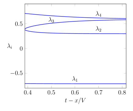
A diagram of Riemann invariants is shown in figure 3. Since in this case we consider a wave propagating in a positive direction, we have $r_{+}^{L}>r_{+}^{R}$, $r_{-}^{L}=r_{-}^{R}$. This means that $\lambda_{4}^{L}>\lambda_{2}^{R}$ and $\lambda_{1}^{L}=\lambda_{1}^{R}$. Then from the constancy of functions $s_{1}$ and $s_{2}$ we get

$$\begin{split}\lambda_{2}^{L}&=\frac{1}{2}\left(\lambda_{2}^{R}+\sqrt{\lambda_{2}^{R}\lambda_{4}^{L}}\right)\\ &=\frac{1}{4}\left(u^{R}+2\sqrt{I^{R}}+\sqrt{(u^{L}+2\sqrt{I^{L}})(u^{R}+2\sqrt{I^{R}})}\right)\end{split}$$ (58)

and

$$\begin{split}\lambda_{4}^{R}&=\frac{1}{2}\left(\lambda_{4}^{L}+\sqrt{\lambda_{2}^{R}\lambda_{4}^{L}}\right)\\ &=\frac{1}{4}\left(u^{L}+2\sqrt{I^{L}}+\sqrt{(u^{L}+2\sqrt{I^{L}})(u^{R}+2\sqrt{I^{R}})}\right).\end{split}$$ (59)

Thus, we know all Riemann invariants on both edges of DSW, that is, we know integrals $s_{1}$ and $s_{4}$ along the whole shock wave. From here we can get the wave velocity and amplitude of the leading soliton

$$\begin{split}\frac{1}{V}&=\frac{s_{1}}{2}=\frac{1}{2}\left(\lambda_{1}^{L}+\lambda_{4}^{L}+\lambda_{2}^{R}+\sqrt{\lambda_{2}^{R}\lambda_{4}^{L}}\right)\\ &=\frac{1}{4}\left(2u^{L}+u^{R}+2\sqrt{I^{R}}\right.\\ &\left.\qquad+\sqrt{(u^{L}+2\sqrt{I^{L}})(u^{R}+2\sqrt{I^{R}})}\right),\end{split}$$ (60)

$$\begin{split}a_{s}&=\frac{1}{4}\left(2\lambda_{4}^{L}-\lambda_{2}^{R}-\sqrt{\lambda_{2}^{R}\lambda_{4}^{L}}\right)\left(\lambda_{2}^{R}-2\lambda_{1}^{L}+\sqrt{\lambda_{2}^{R}\lambda_{4}^{L}}\right)\\ &=I^{L}-\frac{1}{16}\left[2\sqrt{I^{L}}-2u^{L}+u^{R}\right.\\ &\left.\qquad+\sqrt{(u^{L}+2\sqrt{I^{L}})(u^{R}+2\sqrt{I^{R}})}\right]^{2}.\end{split}$$ (61)

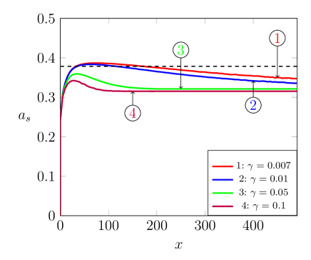
It should be noted that the velocity of the DSW and soliton amplitude depend only on the initial parameters and do not depend on the constant $\gamma$, which reflects the influence of the Raman effect. The numerical results reflecting the dependence of the soliton amplitude on the coordinate $x$ are shown in figure 4. As we can see, there is some deviation of the analytical theory from the numerical calculation, apparently caused by the fact that the Whitham theory does not take into account non-adiabatic effects. It may play a significant role in DSWs theory described by non-integrable equations. Such differences have already been noted in the works egs-06 ; egkkk-07 for other physical systems. Despite this difference, DSW is well described by the Whitham theory, as is illustrated in figure 5. As one can see, the correspondence between the results of Whitham theory and numerical calculations improves noticeably with decrease of the wave amplitude.

Fig. 6: Dispersive shock wave propagating in the negative direction of the $t$-axis for $\gamma=0.1$ with boundary conditions $I_{l}=0.257$, $I_{r}=0.5$, $u_{L}=0.4$ and $u_{R}=0$.

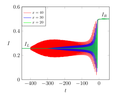
For a wave which propagates in the opposite direction, the reverse situation will occur. Amplitude of oscillations in the wave and its length will continuously increase. The construction of an analytical theory of such a non-stationary nonlinear structure is very difficult and one has to turn to numerical calculation. Figure 6 shows an example of such a wave obtained by numerical solution of the equation (3). It can be seen that the wave profile is significantly different for waves at different distances $x$. In this case, at sufficiently large waveguide lengths $x$, one can see a significant increase in the amplitude of the wave packet separated from the DSW. Description of such a wave packet obeys with good accuracy the linear theory from section 3.

6 Conclusion

In this work, the propagation of sufficiently long pulses in fibers described by the nonlinear Schrödinger equation modified by a small term which characterizes the Raman effect was studied analytically. The main stages of a shock wave formation with an initial profile in the step-like form are considered. Analytical solutions are constructed for the initial unsteady and final stable states using the Whitham method. Perturbed Whitham integrable equations for a nonlinear Schrödinger equation with the Raman term were obtained using the finite-gap integration method.

In principle, one may hope that the results found here can be observed experimentally in systems similar to that used in the recent experiment Xu-2017 . However, one should keep in mind that in standard fibers in addition to the Raman effect, self-steepening effect also occurs. However, the manifestations of these two effects are quite different and therefore they can be identified separately. As shown in the article IvKamch-2017 , the main consequence of self-steepening is the formation of combined shock waves caused by the non-monotonic dependence of the nonlinear term on the wave amplitude, while Raman scattering leads to the formation of stationary shock waves at finite length. At the same time, the Raman effect is usually much stronger than the self-steepening effect. The theory developed in this article shows that the Whitham method provides a general efficient approach for description DSWs in fibers and other optical systems.

Conflict of interest

The authors declare that there is no conflict of interest.

References

W. J. Tomlinson, R. H. Stolen, A. M. Johnson, Optics Lett., 10, 457 (1985).

J. E. Rothenberg, D. Grischkowsky, Phys. Rev. Lett., 62, 531 (1989).

T. B. Benjamin and M. J. Lighthill, Proc. R. Soc. London, Ser. A 224, 448–460 (1954).

R. J. Taylor, D. R. Baker, H. Ikezi, Phys. Rev. Lett., 24, 206 (1970).

R. Z. Sagdeev, Collective processes and shock waves in rarified plasma, in Problems of Plasma Theory, edited by M. A. Leontovich, 1964 (Atomizdat, Moscow, Vol. 5).

A. V. Gurevich and L. P. Pitaevskii, ZhETF, 65, 590 (1973) [Sov. Phys. JETP 38, 291 (1974)].

G. B. Whitham, Proc. Roy. Soc. London, A 283, 238 (1965).

G. B. Whitham, Linear and Nonlinear Waves, Wiley In- terscience, New York, 1974)

G. A. El and M. A. Hoefer, Physica D 333, 11 (2016).

A. V. Gurevich and A. L. Krylov, Sov. Phys. JETP 65, 944 (1987) [Sov. Phys. JETP 92, 1684 (1987)].

G. A. El, V. V. Geogjaev, A. V. Gurevich, A. L. Krylov, Physica D 87, 186 (1995).

G. Xu, M. Conforti, A. Kudlinski, A. Mussot, and S. Trillo, Phys. Rev. Lett., 118, 254101 (2017).

V. E. Zakharov, A. B. Shabat, Sov. Phys. JETP 34, 62-69 (1972) [Sov. Phys. JETP 61, 118—134 (1971)].

W. Wan, S. Jia, and J. W. Fleischer, Nature Phys., 3, 46 (2007).

G. A. El, Chaos 15, 037103 (2005).

G. A. El, A. Gammal, E. G. Khamis, R. A. Kraenkel, A. M. Kamchatnov, Phys. Rev. A 76, 053813 (2007).

X. An, T. R. Marchant, N. F. Smyth, Physica D 342, 45 (2017).

A. M. Kamchatnov, Phys. Rev. E 99, 012203 (2019).

S. K. Ivanov, A. M. Kamchatnov, Phys. Rev. A 96, 053844 (2017).

Y. S. Kivshar, Phys. Rev. A 42, 1757 (1990).

R. S. Johnson, J. Fluid Mech. 42, 49 (1970).

A. V. Gurevich and L. P. Pitaevskii, Zh. Eksp. Teor. Fiz. 93, 871–880 (1987) [Sov. Phys. JETP 66, 490–495 (1987)].

V. V. Avilov, I. M. Krichever, and S. P. Novikov, Dokl. Akad. Nauk SSSR, 295, 345–349 (1987) [Sov. Phys. Dokl., 32, 564–566 (1987)].

A. M. Kamchatnov, Physica D 333, 99 (2016).

A. M. Kamchatnov, Physica D 188, 247 (2004).

P.-É. Larré, N. Pavloff, A. M. Kamchatnov, Phys. Rev. B 86, 165304 (2012).

Yu. S. Kivshar and G. P. Agrawal, Optical Solitons. From Fibers to Photonic Crystals, Academic Press, Amsterdam, 2003.

A. M. Kamchatnov, Nonlinear Periodic Waves and Their Modulations—An Introductory Course, (World Scientific, Singapore, 2000).

G. A. El, R. H. J. Grimshaw, N. F. Smyth, Phys. Fluids, 18, 027104 (2006).