VHE Emission from Magnetic Reconnection in the RIAF of SgrA*

Abstract

The cosmic-ray (CR) accelerator at the galactic centre (GC) is not yet established by current observations. Here we investigate the radiative-inefficient accretion flow (RIAF) of Sagittarius A* (SgrA*) as a CR accelerator assuming acceleration by turbulent magnetic reconnection, and derive possible emission fluxes of CRs interacting within the RIAF (the central $\sim 10^{13}$cm). The target environment of the RIAF is modelled with numerical, general relativistic magneto-hydrodynamics (GRMHD) together with leptonic radiative transfer simulations. The acceleration of the CRs is not computed here. Instead, we inject CRs constrained by the magnetic reconnection power of the accretion flow and compute the emission/absorption of $\gamma$-rays due to these CRs interacting with the RIAF, through Monte Carlo simulations employing the CRPropa 3 code. The resulting very-high-energy (VHE) fluxes are not expected to reproduce the point source HESS J1745-290 as the emission of this source is most likely produced at pc scales. The emission profiles derived here intend to trace the VHE signatures of the RIAF as a CR accelerator and provide predictions for observations of the GC with improved angular resolution and differential flux sensitivity as those of the forthcoming Cherenkov Telescope Array (CTA). Within the scenario presented here, we find that for mass accretion rates $\gtrsim 10^{-7}$M_⊙yr^-1, the RIAF of SgrA* produces VHE fluxes which are consistent with the H.E.S.S. upper limits for the GC and potentially observable by the future CTA. The associated neutrino fluxes are negligible compared with the diffuse neutrino emission measured by the IceCube.

1 Introduction

The dynamic centre of our galaxy has been measured in the very-high-energy (VHE; $>$100 GeV) radiation regime by imaging atmospheric Cherenkov telescopes (IACTs) for over a decade (Tsuchiya et al., 2004; Kosack et al., 2004; Albert et al., 2006; Aharonian et al., 2004, 2009). Particularly, the VHE point-like source J1745-290 measured by the High Energy Stereoscopic System (H.E.S.S.) has been limited within an angular error of 13 arcsec (Acero et al., 2010) at the galactic centre (GC). This limit encloses three plausible astrophysical counterparts within the central $\sim$10 pc: a central spike of annihilating dark matter (Cembranos et al., 2012; Belikov et al., 2012), the pulsar wind nebula (PWN) G359.95-0.04 (Wang et al., 2006), and the supermassive black hole (SMBH) Sagittarius A* (SgrA*) (Aharonian & Neronov, 2005a, b; Atoyan & Dermer, 2004; Fujita et al., 2017).

A hadronic scenario for the origin of J1745-290 has been favoured by measurements of the diffuse VHE emission from the $\sim 200$ pc outskirts of the GC (Aharonian et al., 2006; H.E.S.S. Collaboration et al., 2016). This diffuse emission is spatially correlated with the gas density of the central molecular zone (CMZ) and its emission centroid coincides with the point-like source J1745-290. Such correlations then suggest that both the point-like as well as the diffuse fluxes might be produced by proton-proton (p-p hereafter) interactions of cosmic-rays (CRs) with the gas around the GC. Thus, if the origin of J1745-290 is mostly hadronic, the SMBH SgrA* could be powering CRs acceleration up to PeV energies (Aharonian & Neronov, 2005a, b; H.E.S.S. Collaboration et al., 2016).

No variability in the flux of J1745-290 was found during the simultaneous H.E.S.S. and Chandra observations performed in July 2005, when the X-ray flux of SgrA* increased by a factor of $\sim 9$ (Aharonian et al., 2008). A subsequent analysis with increased statistics of data and improved analysis methods displayed no variability, flaring, or quasi-periodic oscillations in the flux of J1745-290 (Aharonian et al., 2009), and more recently, a monitoring campaign of SgrA* with the MAGIC telescopes reported no significant variability of the emission from this source (Ahnen et al., 2017). This lack of variability disfavours the origin of the bulk emission of the VHE point source within the inner $\sim 100$ gravitational radii around the SMBH SgrA*, where simultaneous flares emitting at X-rays and infrared (IR) bands are most likely produced (Eckart et al., 2004; Dodds-Eden et al., 2009, 2011; Mossoux et al., 2016; Boyce et al., 2018; Okuda et al., 2019).

Another reason to not expect the emission of J1745-290 to be produced within few gravitational radii is the following. CRs leading to a flux compatible with J1745-290 from p-p interactions also produce secondary leptons. If these hadronic interactions take place in a medium with a magnetic field of $\sim$10 G or larger, as in the RIAF of SgrA*, the synchrotron emission of the secondary leptons may overshoot the quiescent X-ray flux from the GC, as shown by Aharonian & Neronov (2005a, b).

The unlikely origin of J1745-290 at few gravitational radii does not exclude however, the possibility of CR acceleration in the immediate vicinity of the SMBH. CRs that escape their acceleration zone could produce the observed emission of J1745-290 further out, while diffusing within the interstellar medium at pc scales, since given the angular resolution of the H.E.S.S. instrument, $\gamma$-rays produced within the central $\sim 10$ pc still appear as point-like emission. This scenario, originally proposed by Aharonian & Neronov (2005b), explains the spectrum of J1745-290 and can be extended to also match the data of the Fermi source 1FGL J1745.6-2900 (e.g., Liu et al., 2006; Chernyakova et al., 2011; Linden et al., 2012).

However, this interpretation as well as the current VHE observations from the GC give no direct information about the specific sites of CR acceleration or the acceleration mechanism. VHE fluxes observed with enhanced angular resolution and differential flux sensitivity like those potentially obtained with the forthcoming CTA (Acharya et al., 2013; Cherenkov Telescope Array Consortium et al., 2017) will be valuable to localise the presumed sites of CR acceleration at the GC.

In this work, we focus on possible VHE fluxes produced within tens of gravitational radii around the SMBH SgrA*. We particularly investigate the scenario of VHE emission produced by hadronic interactions in the accretion flow, where these CRs are accelerated by turbulent magnetic reconnection in the RIAF of SgrA*. In order to explore their detectability and how much they contribute to the current VHE emission from the GC, we compare the derived emission profiles with the differential flux sensitivity of CTA, as well as with the current emission of the source J1745-290.

The acceleration of CRs, and production of neutrinos and non-thermal radiation has been previously discussed in the framework of RIAFs and standard accrection disks considering one-zone models (e.g., de Gouveia Dal Pino et al., 2010a, b; Romero et al., 2010; Khiali et al., 2015; Kimura et al., 2015; Khiali & de Gouveia Dal Pino, 2016).

Particle acceleration by magnetic reconnection has been studied as an important emission process in BH systems, from BH binaries to active galactic nuclei (de Gouveia dal Pino & Lazarian, 2005; Singh et al., 2015; Khiali et al., 2015; Kadowaki et al., 2015; Khiali & de Gouveia Dal Pino, 2016).

The development of magnetic reconnection in accretion flows around BHs has been tested numerically by several authors (e.g., Koide & Arai, 2008; Dexter et al., 2014; Parfrey et al., 2015; Kadowaki et al., 2018; de Gouveia Dal Pino et al., 2018; Ball et al., 2018). In particular, fast reconnection occurrences induced by the magneto-rotational-instability turbulence have been detected in multidimensional general relativistic (GR) magneto-hydrodynamic (MHD) RIAF simulations (de Gouveia Dal Pino et al. 2018; Kadowaki et al. 2019) employing a current-sheet-search algorithm (Kadowaki et al., 2018). Also, stochastic CR Fermi acceleration by turbulent magnetic reconnection has been extensively investigated numerically (Kowal et al. 2011; Kowal et al. 2012; Guo et al. 2016; del Valle et al. 2016; Petropoulou & Sironi 2018; de Gouveia Dal Pino et al. 2019; Werner et al. 2019; see also de Gouveia Dal Pino & Kowal 2015 for a review). Acceleration by reconnection has been also considered recently as a triggering process to allow for further CR stochastic acceleration in MHD simulations of the MRI turbulence in hot accretion flows (Kimura et al., 2019). These authors found that stochastic acceleration is able to energise CRs up to 10 PeV.

In the context of SgrA*, magnetic reconnection has previously been invoked to model its observed IR and X-rays flares (Ball et al., 2016; Li et al., 2017). All these aforementioned results suggest that efficient CR acceleration by magnetic reconnection may occur and produce detectable VHE emission in the vicinity of the SMBH SgrA*.

In our approach, we assume that CRs are accelerated by magnetic reconnection and derive the implied VHE fluxes constraining the total injection of CRs by the magnetic reconnection power of the system. Such predicted VHE fluxes are not expected to coincide with the emission of the point source J1745-290, since as mentioned above, the nature of this source is probably different from the emission produced in the immediate vicinity of the SMBH. Thus, the emission profiles derived here intend to be predictions for future observations with improved angular and energy sensitivity like those of the forthcoming CTA.

In the next section, we describe the numerical GRMHD simulation and the GR radiative transfer calculations that we employ to model the accretion flow environment where CRs interact. The interactions and emission of CRs in the accretion flow are simulated with a Monte Carlo approach that we describe in Section 3. In Section 4, we describe and discuss different simulated models for the VHE fluxes associated to different values of the mass accretion rate. Finally, we present our conclusions in Section 5.

2 The numerical GRMHD model for accretion plasma environment

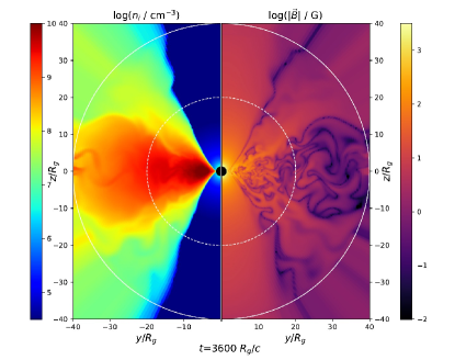
Figure 1: Gas number density and magnetic field intensity maps corresponding to a snapshot at the time evolution $t=3600R_{g}/c$ of the accretion flow simulation described in Section 2, employing the axis-symmetric harm code. The inner white circle represents the spherical boundary of CR injection and the outer circle the boundary for $\gamma$-ray detection in the CR simulations described in Section 3.

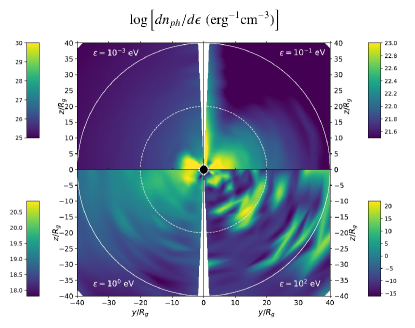
Figure 2: Photon field maps of synchrotron plus inverse Compton radiation corresponding to the accretion flow snapshot of Fig. 1, calculated with the grmonty code assuming the proton-to-electron temperature ratio of $T_{p}/T_{e}=80$. The photon field is shown at different energy bands in each panel, as indicated.

Due to its bolometric luminosity and accretion rate constrained by observations, the emitting material of SgrA* has been classified as a RIAF (Narayan et al., 1995; Yuan et al., 2003; Yuan & Narayan, 2014). In this work we consider that CRs potentially accelerated by turbulent magnetic reconnection in the accretion flow (e.g., Singh et al. 2015) will first interact within the RIAF environment before escaping to the outer regions. To model the gas density, magnetic and photon fields profiles of the plasma, we employ the GRMHD axi-symmetric harm code (Gammie et al., 2003; Noble et al., 2006) together with the GR radiative transfer grmonty code (Dolence et al., 2009).

We consider a numerical simulation where the accretion is triggered by magneto-rotational instability on a torus initially in hydrostatic equilibrium (Fishbone & Moncrief, 1976), similar to the studies by e.g., Mościbrodzka et al. (2009), Davelaar et al. (2018), Jiménez-Rosales & Dexter (2018), and other authors. The initial torus of the simulation has an inner radius at $6R_{g}$, a maximum gas pressure at $12R_{g}$, and is threaded with a poloidal magnetic field following the iso-density contours with a minimum plasma beta $\beta=50$. We use the dimensionless spin parameter $a=0.94$, the gas specific heat ratio $\gamma=4/3$, and a 256x256 resolution for the $R$ and $\theta$ spherical coordinates.

The soft radiation field, $n_{ph}$, of the accretion flow is calculated with post-processing radiative transfer (i.e., assuming that radiation pressure is not important in the plasma dynamics) of synchrotron plus inverse Compton radiation. The emitting electrons are assumed to follow a relativistic Maxwellian distribution where their temperature is a fraction of the ions temperature. The photon field is then obtained by calculating the radiation flux with the grmonty code at different radius and polar angles within the accretion flow zone.

The physical values of the gas density and the magnetic field profiles are obtained as $\rho=\rho_{0}\rho^{\prime}$, $B_{i}B^{i}=B_{0}^{2}B^{\prime}_{i}B^{\prime i}$, respectively, where $\rho^{\prime}$ and $B^{\prime i}$ are the gas density and the 3-magnetic field in code units. In these code units, the gas density is normalised so that $\rho^{\prime}=1$ at the maximum pressure of the initial torus.

Given a fixed value for the density normalisation factor $\rho_{0}$, the normalisation factor for the magnetic field is determined as $B_{0}=c\sqrt{4\pi\rho_{0}}$. This defines the accretion flow characteristics in physical units for each snapshot (Fig. 1 depicts one of these snapshots from our simulation, see more below).

The photon field density for each of these snapshots is obtained at the different points of the axi-symmetric flow as:

$$\frac{dn_{ph}}{d\epsilon}=\frac{\nu L_{\nu}(R,\theta,\epsilon,T_{p}/T_{e})}{4\pi c\epsilon^{2}R^{2}}\,,$$ (1)

where the differential luminosity $L_{\nu}$ is provided by the radiative transfer calculation at different radii and polar angles (Fig. 2). The value of the proton-to-electron temperature ratio, $T_{p}/T_{e}$, used to obtain the photon field of a given snapshot is chosen such that the calculated spectral energy distribution (SED) due to synchrotron plus IC is consistent with the observed radio to IR data of SgrA* (see Fig. 3).

Summarising, the spatial profiles of $\rho$, $B^{i}$ and $n_{ph}$ (gas density, magnetic field, and soft photon field) in the accretion flow are given by the GRMHD + GR radiative transfer simulations which are normalised by arbitrarily choosing the gas density unit $\rho_{0}$ together with the constraint of the radio-IR data of SgrA* (to define the value of the ratio $T_{p}/T_{e}$). Equivalently, we can freely choose the mass accretion rate and then define the normalisation factors $\rho_{0}$, $B_{0}$, and $T_{p}/T_{e}$.

In Fig. 1, we show the gas number density and magnetic field maps corresponding to the snapshot $t=3600\,R_{g}/c$ of the simulation as described in this section. The physical units of the maps in Fig. 1 are obtained using the gas density normalisation factor of $\rho_{0}=1.59\times 10^{10}$ cm^-3.

In Fig. 2 we show the photon field maps associated to the snapshot of Fig. 1, assuming $T_{p}/T_{e}=$80.

In the next section, we consider three different RIAF background models, each one obtained by choosing a different gas density normalisation, as described. For each background model, we calculate the emission of CRs injected in the accretion flow during a total time interval $\Delta t=320R_{g}/c$ that encompasses four subsequent snapshots of the simulation, namely $t=3440,3520,3600$, and $3680\,R_{g}/c$, in order to mimic a continuous injection of CRs.

In Fig. 3, we show the SEDs (averaged over these four snapshots) due to leptonic synchrotron plus IC emission for the three background models, each one labelled with the corresponding mass accretion rates and temperature ratios.

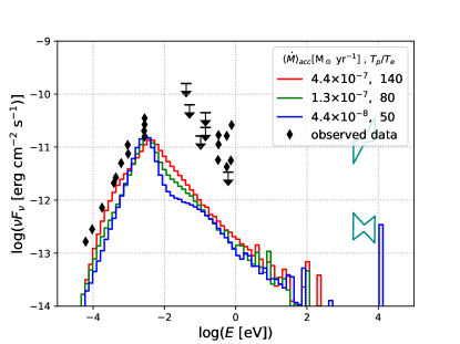
Figure 3: SED distribution due to synchrotron plus IC emission of the BH accretion flow calculated with the grmonty code for three models with different mass accretion rates and proton to electron temperature ratio (i.e. with different density normalisation). Each histogram gives the average leptonic SED obtained out of four snapshots of the accretion flow (see text). The data points correspond to the observed SED of SgrA*, adapted from Mościbrodzka et al. (2009).

3 Monte Carlo simulation of cosmic-ray emission

CRs accelerated in the RIAF of SgrA* by magnetic reconnection (see Section 4) produce $\gamma$-ray fluxes due to their interactions with the gas density, magnetic, and photon fields of the accretion flow environment. Whether these interactions are efficient enough to produce detectable $\gamma$-ray fluxes depends on the parameters of the accretion flow as well as on power and spectrum of the injected protons. We investigate this potential hadronic $\gamma$-ray emission by simulating the propagation and interaction of CRs and their secondaries with an extended version of the Monte Carlo code CRPropa 3 (Alves Batista et al., 2016). In these simulations, we assume that CRs are composed only by protons and we consider (i) proton-proton interactions of CRs with the thermal background ions, (ii) photon-pion interactions of CRs with the background soft photon field, (iii) $\gamma$-$\gamma$ absorption of VHE photons by the background soft photon field with production of electron-positron pairs, (iv) inverse Compton scattering of secondary leptons produced in the previous interactions, and (v) synchrotron cooling to account for energy losses of charged particles. Note that we do not track synchrotron photons as their energies are much lower than $\sim$ 1 GeV.

CRPropa simulates 3D trajectories of charged particles by solving the relativistic Lorentz force equation in a flat space-time. In our approach, we take the magnetic field 3-vector $B^{i}$ given by the axi-symmetric snapshots of the GRMHD simulation (see Section 2), rotate it to produce a magnetic field defined in a 3D uniform grid, and use it in a flat spacetime without any further transformations to perform the simulation of 3D CR propagation. The error introduced by neglecting GR effects in the trajectory of the CRs and photons in the resulting VHE emission decreases for $\gamma$-rays produced at larger distances from the central BH (In Appendix B, we show the radial distribution for the production of VHE photons, for chosen emission models derived in Section 4).

CRPropa 3 simulates the interactions of particles and photons along their trajectories using a Monte Carlo method and pre-loaded lookup tables for the interaction rates. For our calculations, we implement into the code spatially-dependent interaction mean free paths (MFPs) calculated out of the gas density and photon field profiles of the GRMHD snapshots. Thus, the MFP for proton-proton interactions $\lambda_{pp}$, photo-hadronic interactions $\lambda_{p\gamma}$, photon-photon pair creation $\lambda_{\gamma\gamma}$, and inverse Compton scattering $\lambda_{IC}$, are calculated as:

$$\lambda_{pp}^{-1}(E_{p},R_{i},\theta_{j})=\sigma_{pp}(E_{p})n_{i}(R_{i},\theta_{j}),$$ (2)

$$\begin{split}\lambda^{-1}_{p\gamma}(E_{p},R_{i},\theta_{j})&=\frac{m_{p}^{2}c^{4}}{2E_{p}^{2}}\int_{0}^{\infty}d\epsilon\\ &\times\frac{n_{ph}(\epsilon,R_{i},\theta_{j})}{\epsilon^{2}}\int_{145MeV}^{\frac{2E_{p}\epsilon}{m_{p}c^{2}}}d\epsilon^{\prime}\epsilon^{\prime}\sigma_{p\gamma}(\epsilon^{\prime})\,,\end{split}$$ (3)

$$\begin{split}\lambda^{-1}_{\gamma\gamma}(E_{\gamma},R_{i},\theta_{j})&=\frac{1}{8E_{\gamma}^{2}}\int_{2m_{e}^{2}c^{4}}^{4E_{\gamma}\epsilon_{max}}ds\\ &\times s\sigma_{\gamma\gamma}(s)\int_{0}^{\infty}d\epsilon\frac{n_{ph}(\epsilon,R_{i},\theta_{j})}{\epsilon^{2}},\end{split}$$ (4)

$$\begin{split}\lambda^{-1}_{IC}(E_{e},&R_{i},\theta_{j})=\frac{1}{8\beta E_{e}^{2}}\int_{m_{e}^{2}c^{4}}^{m_{e}^{2}c^{4}+E_{e}\epsilon_{max}(1+\beta)}ds\\ &\times\sigma_{IC}(s)(s-m_{e}^{2}c^{4})\int_{0}^{\infty}d\epsilon\frac{n_{ph}(\epsilon,R_{i},\theta_{j})}{\epsilon^{2}}.\end{split}$$ (5)

In equations (2)-(5), $n_{i}(R_{i},\theta_{j})$ and $n_{ph}(R_{i},\theta_{j},\epsilon)$ are the gas number density and the photon field at discrete spatial points. $E_{p}$, $E_{e}$, and $E_{\gamma}$ are the energies of protons, leptons, and $\gamma$-rays, respectively, and $m_{p}$ and $m_{e}$ the proton and electron mass, respectively. $\sigma_{pp}$, $\sigma_{p\gamma}$, $\sigma_{\gamma\gamma}$, and $\sigma_{IC}$ are the cross sections for the proton-proton interaction, photopion production, photon-photon pair production and inverse Compton scattering, respectively. In the integral of equation (5) $\beta=\sqrt{1-m_{e}^{2}c^{4}/E_{e}^{2}}$.

Because CRPropa does not perform proton-proton interactions, we have implemented it using the parametrisation for $\sigma_{pp}$ from Kafexhiu et al. (2014). The fraction of the parent’s energy taken by secondary particles is estimated using parametrisations from Kelner et al. (2006). The expressions for the cross sections $\sigma_{\gamma\gamma}$ and $\sigma_{IC}$ can be found in Alves Batista (2015) (see also Kachelrieß et al. 2012 and Lee 1998). The MFPs of Eqs. (3)-(5) are calculated employing the CRPropa tools, that we modify in order to include the information of the gas density $n_{i}(R_{i},\theta_{j})$ and the photon field $n_{ph}(\epsilon,R_{i},\theta_{j})$.

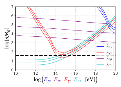
Figure 4: Interaction mean free paths for particles and photons, in units of the gravitational radius of SgrA*. The size of the accretion flow zone ($40R_{g}$) is indicated by the thick, dashed, black line. The interactions are calculated with the gas density and photon field obtained from the numerical GRMHD snapshot displayed in Figs. 1 and 2. For the photon-pion ($\lambda_{p\gamma}$), pair production ($\lambda_{\gamma\gamma}$), and inverse Compton ($\lambda_{IC}$) interactions, the different curves are calculated at the $\theta=45^{\mbox{\tiny{o}}}$ polar angle, and at 20 (lower-most lines), 30 (middle), and 40 $R_{g}$ (upper-most) from the central BH. For the proton-proton interaction ($\lambda_{pp}$) the different curves are calculated with the maximum gas density (lower-most), and with 0.1 (middle), and 0.01 (upper-most) fractions of the maximum gas density.

In Fig. 4, we show these interaction MFPs as a function of the energy, calculated with the gas density and the photon field of the GRMHD snapshot of Figs. (1)-(2). Although in the next section we consider different accretion flow backgrounds where the associated MPF curves are slightly different, the example shown in Fig. 4 qualitatively describes the overall behaviour of the interactions for all the background models considered in this work. We see that protons with energies $\lesssim 10^{15}$ eV produce $\gamma$-rays principally due to proton-proton interactions; $\gamma$-ray absorption by pair creation is significant for $\gamma$-rays with energies within $\sim 10^{13}$-$10^{18}$ eV; and $\gamma$-rays produced due to IC scattering are mainly produced by secondary leptons with energies $\lesssim 10^{14}$ eV. We note that $\gamma$-rays with energies $\lesssim 10^{13}$ eV readily escape the RIAF of SgrA*, as previously discussed by Aharonian & Neronov (2005a). The production of $\gamma$-rays due to photo-hadronic processes within the RIAF is significant for protons with energies $\gtrsim 10^{18}$ (ultra-high-energy cosmic-rays). However, in all models of this work we assume that the energies of the accelerated CRs are lower than $\sim 10^{15}$ eV (see Section 4), and thus, photo-hadronic interactions are not expected to significantly contribute to the production of $\gamma$-rays.

To calculate the emission due to a continuous injection of CRs, we employ four different snapshots with 80 $R_{g}/c$ time separation between each other, and simulate a burst-like propagation of CRs in each one. We inject in each burst CRs with a power-law energy distribution with power-law index $\kappa$, and exponential energy cut-off $\epsilon_{cut}$:

$$\frac{dN_{CR}}{d\epsilon}\propto\epsilon^{-\kappa}\exp\{-\epsilon/\epsilon_{cut}\}.$$ (6)

The energy of injected CRs in each snapshot is $E=W_{CR}\Delta t/4$, where $\Delta t=320R_{g}/c$ is the total injection time interval and $W_{CR}$ is the CR injection power.

The simulations are performed with $10^{6}$ protons, with initial position and momentum isotropically distributed within a sphere of $20R_{g}$ (represented as the inner dashed circle in Figs. 1-2) and we track photons and particles until they attain a minimum energy of $10^{11}$eV, or they complete a trajectory length of $160R_{g}$ (initiated from the parent protons), or else they cross a spherical detection boundary at $40R_{g}$ (represented as the outer circle in Figs. 1-2) from the central BH. In Appendix A we describe in detail how we calculate the SED of the $\gamma$-rays from the output data of the simulations. In the next section we describe the VHE emission models obtained from CRs interacting in different background models, where the CR injection is constrained to the available magnetic reconnection power of the background accretion flow.

4 VHE fluxes from the RIAF of SgrA*

Table 1: Parameters of the emission profiles plotted in Fig. 5.

Model	$\langle\dot{M}_{acc}\rangle\times 10^{-7}$ [M⊙ yr-1]	$T_{p}/T_{e}$	$W_{CR}\times 10^{37}$[erg s-1]	$W_{CR}/W_{rec}$	$\kappa$	$\epsilon_{cut}$ [PeV]
m11	$4.452$	140	30	0.8	2.4	0.05
m12	$4.452$	140	2	0.05	1.8	0.5
m13	$4.452$	140	0.8	0.02	1.3	0.5
m21	$1.335$	80	6.5	1.0	1.8	0.05
m22	$1.335$	80	6	0.92	1.8	0.5
m23	$1.335$	80	3	0.46	1.3	0.5
m31	$0.445$	50	1.3	0.96	1.0	0.05
m32	$0.445$	50	1.3	0.96	1.0	0.5

As described, we consider three background RIAF models and calculate their VHE fluxes. Each background model (i.e. the gas density and the magnetic and photon fields of the accretion flow) is defined by choosing the value of the gas density normalisation, $\rho_{0}$, for the snapshots of the GRMHD simulation, and fixing the proton-to-electron temperature ratio, $T_{p}/T_{e}$, to obtain the photon field which is constrained by the radio-IR data of SgrA* (see Section 2). The magnetic reconnection power of a particular background model to accelerate the CRs, is obtained following the analytic model for magnetic reconnection in magnetically-dominated accretion flows (MDAFs) of Singh et al. (2015) (see also de Gouveia dal Pino & Lazarian 2005; Kadowaki et al. 2015):

$$W_{rec}=1.52\times 10^{42}f\left(\frac{\langle\dot{M}_{acc}\rangle}{\mbox{M}_{\odot}\mbox{yr}^{-1}}\right)\left(\frac{T_{p}}{T_{e}}\right)\,\mbox{erg s}^{-1},$$ (7)

where $\langle\dot{M}_{acc}\rangle$ is the average accretion rate over the four snapshots employed for the calculation of the CR emission (see Sections 2-3 and Appendix A), the factor $f$ is a combination of dimensionless parameters and here we adopt a fiducial value $f=4$. The basic assumption of this work is that the energy of the CRs accelerated in the RIAF is provided by magnetic reconnection, as described in Section 1. Thus, to calculate the VHE emission in the background models, we constrain the power of CR injection, $W_{CR}$, with the condition $W_{CR}/W_{rec}<1$.

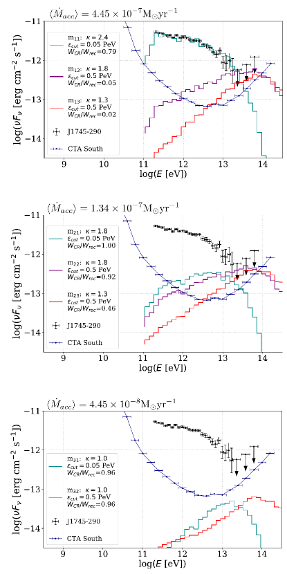
Figure 5: SED of hadronic emission produced by CRs accelerated by magnetic reconnection within the RIAF of SgrA* and calculated with the CRPropa 3 code (see the text). Additional parameters of the emission profiles can be found in Table 1. In each panel we over-plot the data points of the source HESS J1745-290, adapted from H.E.S.S. Collaboration et al. (2016), and the differential flux sensitivity of the forthcoming CTA, adapted from Cherenkov Telescope Array Consortium et al. (2017)

Fig. 5 shows the calculated SED of the accretion flows with different accretion rates, and the parameters obtained for the plotted emission profiles are listed in Table 1.

The emission curves in the upper panel of Fig. 5 correspond to a background accretion flow with $\langle\dot{M}_{acc}\rangle=4.452\times 10^{-7}$ M_⊙ yr^-1. The emission profile of model m₁₁ in this diagram is obtained injecting CRs with a power-law index $\kappa=2.4$ and exponential cut-off energy $\epsilon_{cut}=5\times 10^{13}$ eV. This emission profile matches quite well the VHE data of the point source J1745-290. However, as we mention in the introduction, such a VHE flux produced out of proton-proton interactions also implies an X-ray flux (due to the synchrotron emission of the secondary leptons produced through the channel $p$+$p\rightarrow\pi^{\pm}\rightarrow$ e^±) that overshoots by $\sim$ one order of magnitude the quiescent X-ray emission of SgrA* (Aharonian & Neronov, 2005b, a). This overestimation would not be conflicting if the flux of J1745-290 corresponded to flare episodes coincident with those measured at X-rays energies from SgrA*. However, as mentioned in the introduction, variability, flaring, or QPOs have not been found in the flux of the source J1745-290 (Aharonian et al., 2008, 2009). In contrast, the emission profile of the model m₁₂ obtained with CRs injected with the power-law index $\kappa=1.8$ and cut-off energy $\epsilon_{cut}=0.5$ PeV produces a flux within the RIAF of SgrA* that matches the upper limits detected by H.E.S.S. in the VHE tail. This emission profile peaks at $\sim 10^{13.5}$ eV with a flux one order of magnitude lower than the peak of the model m₁₁ and thus does not overshoot the quiescent emission at X-ray energies. Also, it requires $\sim$5% of the reconnection power, and is above the differential flux sensitivity of the future CTA in the energy range of $10^{12-14}$ eV. The emission profile of the model m₁₃ corresponds to CRs injected with the power-law index $\kappa=1.3$ and cut-off energy $\epsilon_{cut}=0.5$ PeV. This emission model requires $2\%$ of the reconnection power and is also above the CTA sensitivity.

The emission curves in the middle panel of Fig. 5 correspond to CRs emitting within a background with accretion rate of $\langle\dot{M}_{acc}\rangle=1.33\times 10^{-7}$ M_⊙ yr^-1. In this case, the magnetic reconnection power is not sufficient to reproduce the bulk emission of the source J1745-290 with any configuration of the parameters $W_{CR}$, $\kappa$, and $\epsilon_{cut}$. The curve from model m₂₁ is produced with CRs injected with the power-law index $\kappa=1.8$ and cut-off energy $\epsilon_{cut}=5\times 10^{13}$ eV, and peaks at $\sim 10^{12.5}$ eV with a flux of $10^{-12.5}$ erg cm^-2 s^-1. This flux profile makes no substantial contribution to the current data of the source J1745-290, but is, in principle, detectable by the future CTA. The flux models m₂₂ and m₂₃ correspond to CR injection with the same values of $\kappa$ and $\epsilon_{cut}$ of the models m₁₂ and m₁₃, respectively, and they are also qualitatively similar to their counterparts. They differ in that the models m₂₂ and m₂₃ require a larger fraction of the available magnetic reconnection power, which is naturally expected since the rate of proton-proton interactions as well as the magnetic reconnection power diminish for lower accretion rate (see Eq. 7).

Finally, it is shown in the lower panel of Fig. 5 that the VHE fluxes produced by RIAFs with accretion rates of $\langle\dot{M}_{acc}\rangle=4.45\times 10^{-8}$ M_⊙ yr^-1 and lower are not detectable.

Thus, based in the flux profiles of Fig. 5, we conclude that magnetic reconnection in the RIAF of SgrA* powers VHE fluxes that can be potentially detected by CTA, provided that the mass accretion rate is $\langle\dot{M}_{acc}\rangle\gtrsim 10^{-7}$ M_⊙ yr^-1. With regard to the expected fraction of the magnetic reconnection power that should be available for CR acceleration, laboratory experiments of reconnection (Yamada et al., 2010) and PIC simulations (e.g., Werner & Uzdensky 2017) predict that 30% to 50% goes into particle acceleration and the remaining goes to heat the plasma. In this sense, models m₁₂, m₁₃, and m₂₃ would be more favorable solutions.

In Fig. 6, we show the neutrino fluxes associated to the emission models m₁₁, m₁₂, m₁₃, m₂₁, m₂₂ and m₂₃ of Fig. 5. We see that the neutrino emission produced within the accretion flow of SgrA* is practically negligible compared to the IceCube diffuse neutrino flux.

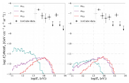
Figure 6: All-flavour neutrino fluxes associated to the emission profiles of the upper and middle panels of Fig 5. The IceCube high-energy starting events are taken from Aartsen et al. (2015).

As mentioned in Section 3, the error introduced by using the background environment of the GRMHD simulation in a flat spacetime and neglecting the GR curvature effects on the propagation of CRs and VHE photons, is lower for $\gamma$-rays produced at larger distances from the central BH. In Appendix B, we show that photons with energies $\gtrsim 10$ TeV, are more uniformly sourced within the 40$R_{g}$ volume than photons with lower energies. This is because lower energy photons are produced by lower energy CRs which have smaller Larmor radii and then are more easily trapped close to the BH where the magnetic field is more intense. Thus, we conclude that the error of neglecting the GR effects in the calculation of the VHE emission is lower for the emission models m₁₂, m₁₃, m₂₂, and m₂₃, which peak at energies $>10$ TeV. A more consistent approach considering the GR curvature effects on the propagation of CRs and VHE photons (possibly by following the approach of Bacchini et al. 2019) is left for future work.

In axy-symmetric numerical GRMHD RIAFs, strong magnetic reconnection events are localised mostly within the turbulent torus and in the interfaces between inflows and outflows, where several magnetic field reversals are identified, as can be seen in (de Gouveia Dal Pino et al., 2018) and (Kadowaki et al., 2019), where a fast magnetic reconnection tracking algorithm (Kadowaki et al., 2018) is employed. Because in this work we do not analyse the details of the magnetic reconnection sites produced by the simulated accretion flow, we injected isotropically the accelerated CRs within a sphere of 20$R_{g}$, where the magnetic fields take the highest values (see Section 3). If alternatively the CR injection is limited to the region of the accreting torus, the flux of the VHE emission is increased by a factor of $\sim$2, as can be seen in Fig. 7. This is expected, as the same CR injection power that had previously expanded throughout the sphere is now injected in the denser region of the flow (the torus region). Thus, the overall rate of p-p interactions is slightly increased and so the overall gamma-ray emission. As a consequence, there is no relevant difference between the spherical and the torus-limited injections in the resulting SED profiles.

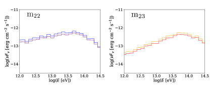
Figure 7: Calculated SEDs corresponding to the models m₂₂ and m₂₃ (see Table 1) for two different CR injection configurations. The purple and red curves correspond to CR injection homogeneously distributed within a sphere of $20R_{g}$ (as in Fig. 5). The blue and orange curves correspond to CR injection with the same model parameters, but weighting the previous simulation output to limit the CR injection within the volume defined by the polar angle range $\theta\in[\pi/4,3\pi/4]$ and the spherical radius range $r\in$[2$R_{g}$, 20$R_{g}$].

5 Conclusions

Point-like as well as diffuse VHE emission measured at the GC suggest the existence of a PeVatron in the direction of SgrA*. The site (or sites) of CR acceleration has not yet been determined by observations with the current IACTs. Future observations with the sensitivity of the forthcoming CTA may provide more localised VHE fluxes able to trace the real sites of CR acceleration.

In this work, we investigate the RIAF of SgrA* as a potential PeVatron, assuming that CRs are accelerated by turbulent magnetic reconnection and we then derive the implied VHE emission fluxes produced exclusively within the accretion flow plasma. Our approach is based on:

• numerical GRMHD plus GR radiative transfer, to model the RIAF environment of SgrA*,

• CRs injection constrained by the magnetic reconnection power of the system which we calculate following the model of (Singh et al., 2015), and

• MC simulations of CRs propagation plus electromagnetic cascading, to calculate the VHE $\gamma$-ray emission produced within the accretion flow environment.

We calculate the emission of CRs interacting with accretion flows considering three different mass accretion rates. Constraining the injection of CRs to the magnetic reconnection power, we find that systems with mass accretion rates $\gtrsim 10^{-7}$ M_⊙ yr^-1 produce VHE fluxes which are compatible with the highest energy upper limits by H.E.S.S. and that could be potentially observed by CTA.

For CR injection with power-law indices $\kappa=1.3-1.8$ and exponential cut-off energy $\epsilon_{cut}=0.5$ PeV (which are parameters consistent with particle acceleration by reconnection), such emission profiles peak at $\sim 10^{13.5}$ eV and have no substantial contribution to the current data points of the source J1745-290 (see the curves of the models m₁₂, m₁₃, m₂₂ and m₂₃ in Fig. 5).

The neutrino fluxes associated to these emission profiles are negligible compared with the IceCube neutrino diffuse emission.

The mass accretion rate threshold for detectable VHE fluxes derived here coincides with the upper limit for the mass accretion rate of SgrA* inferred from rotation measures (Marrone et al., 2007). Thus, if fluxes similar to the emission profiles of models m₂₂ and m₂₃ (see Fig. 5) are detected, they might be correlated with episodic enhancements in the accretion rate of SgrA*.

Appendix A Calculation of the VHE SED

We calculate the energy flux of $\gamma$-rays within the energy bin $\epsilon$ measured at the Earth as

$$\nu F_{\nu}=(4\pi R_{s}^{2})^{-1}\epsilon^{2}\frac{\dot{N}_{\epsilon}}{\Delta\epsilon},$$ (A1)

where $R_{s}=7.9$ kpc is the distance from SgrA* to us, $\Delta\epsilon$ is the size of the energy bin, and $\dot{N}_{\epsilon}$ is the number of photons per unit time with energies between $\epsilon$ and $\epsilon+\Delta\epsilon$ that reach the spherical detection boundary at $40R_{g}$ (as a result of the hadronic interactions plus $\gamma$-$\gamma$/IC cascading simulated with the CRPropa 3 code, see Section 3).

As described in Section 3 (see also Rodríguez-Ramírez et al. 2019), we emulate a continuous release of CRs by the RIAF of SgrA* during a time interval $\Delta t$ by injecting CRs at equally separated times $t_{i}$ (see Section 3) within the interval $\Delta t$ that contains four nearly steady state snapshots of the background accretion flow. Thus, the rate of $\gamma$-rays leaving the detection boundary is calculated as

$$\dot{N}_{\epsilon}=\frac{1}{\Delta t}\sum\limits_{i=1}^{4}N_{\epsilon,i},$$ (A2)

where $\Delta t$ is the time interval for photon detection (the same interval for CR injection), and $N_{\epsilon,i}$ are the number of photons within the energy bin $\epsilon$, produced by CRs injected at the time $t_{i}$.

To save computational resources, we inject $10^{6}$ CRs at each injection time $t_{i}$. This number of simulated CRs is several orders of magnitude smaller than the number of physical CRs expected in the physical system. Thus, we calculate the physical number of detected $\gamma$-rays, $N_{\epsilon,i}$, assuming statistical convergence with the condition:

$$N_{\epsilon,i}=\sum_{\epsilon_{0}}\left(\frac{N_{CR,\epsilon_{0},i}}{N_{CR,\epsilon_{0},i}^{sim}}\right)N^{sim}_{\epsilon(\epsilon_{0}),i},$$ (A3)

where the factor in the parenthesis is the ratio of physical to simulated CRs within the energy bin $\epsilon_{0}$, and $N_{\epsilon(\epsilon_{0})}^{sim}$ is the number of photons in the output of the simulation within the energy bin $\epsilon$ that was ultimately produced by CRs injected with initial energy within the energy bin $\epsilon_{0}$.

The CR simulations are performed with power-law injection distribution of index 1. Thus to calculate the flux of physical gamma rays corresponding to the injection of physical CRs with arbitrary power-law distribution $\kappa$, we normalise the distribution of the injected physical CRs ($N_{CR,\epsilon_{0},i}\propto\epsilon_{0}^{-\kappa}\exp\left\{-\epsilon_{0}/\epsilon_{cut}\right\}$), with the physical energy of CR injection $E_{i}$, and the distribution of simulated CRs ($N_{CR,\epsilon_{0},i}^{sim}\propto\epsilon_{0}^{-1}$), with the total number of simulated CRs $N_{CR}$. Then, the ratio in parenthesis in Eq. A3 is expressed in terms of the physical energy of CRs injection $E_{i}$, and the number of simulated CRs $N_{CR}$ as

$$\frac{N_{CR,\epsilon_{0},i}}{N^{sim}_{CR,\epsilon_{0},i}}=\frac{E_{i}}{N_{CR,i}}\frac{\ln(\epsilon_{max}/\epsilon_{min})}{\int_{\epsilon_{min}}^{\infty}\epsilon^{1-\kappa}\exp\{-\epsilon/\epsilon_{cut}\}d\epsilon}\epsilon_{0}^{1-\kappa}\exp\left\{-\epsilon_{0}/\epsilon_{cut}\right\}.$$ (A4)

For simplicity we consider the same amount of energy of the physical CRs in each injection time $E_{i}=W_{CR}\Delta t/4$, being $W_{CR}$ the power of physical CRs, assumed to be constant during the time interval $\Delta t$. Finally, combining Eqs. A3 and A4, the rate of physical photons $\dot{N}_{\epsilon}$ can be expressed in terms of the power of CR injection, $W_{CR}$, as

$$\dot{N}_{\epsilon}=W_{CR}\frac{\ln\left(\epsilon_{max}/\epsilon_{min}\right)}{\int_{\epsilon_{min}}^{\infty}\epsilon_{0}^{1-\kappa}\exp\{-\epsilon_{0}/\epsilon_{cut}\}d\epsilon_{0}}\sum\limits_{i=1}^{4}\sum\limits_{\epsilon_{0}}\frac{1}{N_{CR,i}}\epsilon_{0}^{1-\kappa}\exp\{-\epsilon_{0}/\epsilon_{cut}\}N_{\epsilon(\epsilon_{0}),i}^{sim}\;.$$ (A5)

Appendix B Radial location of the production of VHE photons

As described in Section 3, we use the gas density, magnetic and photon fields obtained with the GRMHD and GR leptonic radiative transfer simulations, to set the environment in a flat spacetime where we perform CR and VHE photon propagation. The error introduced by this in the calculation of the overall VHE flux depends on the location where the photons are sourced.

We show in Fig. 8, the distribution of photons for different energy ranges, as a function of the distance from the central BH where they were produced. The distributions in these plots correspond to the emission models m₂₁, m₂₂, m₂₃ (the model parameters are in Table 1 of Section 4). We can see that the origin of photons is more uniformly distributed along the 40 $R_{g}$ volume for models m₂₂ and m₂₃ and for photons with energy 10$<E/TeV<$100. The origin of photons with energies $<$1 TeV seems to be mostly sourced at distances $\lesssim 20R_{g}$ from the BH. We then conclude that emission profiles peaking at energies $\gtrsim 10$ TeV like the emission profiles m₁₃ and m₂₃ (see Fig. 5) appear to have the lowest error due to the neglection of the GR curvature effects in the calculation of the VHE SED.

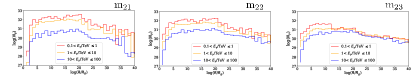
Figure 8: Distribution of photons as a function of their origin distance to the central BH, for different energy ranges. Each panel corresponds to the labelled model emission (see text).

References

- Aartsen et al. (2015) Aartsen, M. G., Abraham, K., Ackermann, M., et al. 2015, ApJ, 809, 98
- Acero et al. (2010) Acero, F., Aharonian, F., Akhperjanian, A. G., et al. 2010, MNRAS, 402, 1877
- Acharya et al. (2013) Acharya, B. S., Actis, M., Aghajani, T., et al. 2013, Astroparticle Physics, 43, 3
- Aharonian & Neronov (2005a) Aharonian, F., & Neronov, A. 2005a, ApJ, 619, 306
- Aharonian & Neronov (2005b) —. 2005b, Ap&SS, 300, 255
- Aharonian et al. (2004) Aharonian, F., Akhperjanian, A. G., Aye, K.-M., et al. 2004, A&A, 425, L13
- Aharonian et al. (2006) Aharonian, F., Akhperjanian, A. G., Bazer-Bachi, A. R., et al. 2006, Nature, 439, 695
- Aharonian et al. (2008) Aharonian, F., Akhperjanian, A. G., Barres de Almeida, U., et al. 2008, A&A, 492, L25
- Aharonian et al. (2009) Aharonian, F., Akhperjanian, A. G., Anton, G., et al. 2009, A&A, 503, 817
- Ahnen et al. (2017) Ahnen, M. L., Ansoldi, S., Antonelli, L. A., et al. 2017, A&A, 601, A33
- Albert et al. (2006) Albert, J., Aliu, E., Anderhub, H., et al. 2006, ApJ, 638, L101
- Alves Batista (2015) Alves Batista, R. 2015, PhD thesis, U. Hamburg, Dept. Phys., doi:10.3204/DESY-THESIS-2015-013
- Alves Batista et al. (2016) Alves Batista, R., Dundovic, A., Erdmann, M., et al. 2016, J. Cosmology Astropart. Phys, 5, 038
- Atoyan & Dermer (2004) Atoyan, A., & Dermer, C. D. 2004, ApJ, 617, L123
- Bacchini et al. (2019) Bacchini, F., Ripperda, B., Porth, O., & Sironi, L. 2019, ApJS, 240, 40
- Ball et al. (2016) Ball, D., Özel, F., Psaltis, D., & Chan, C.-k. 2016, ApJ, 826, 77
- Ball et al. (2018) Ball, D., Özel, F., Psaltis, D., Chan, C.-K., & Sironi, L. 2018, ApJ, 853, 184
- Belikov et al. (2012) Belikov, A. V., Zaharijas, G., & Silk, J. 2012, Phys. Rev. D, 86, 083516
- Boyce et al. (2018) Boyce, H., Haggard, D., Witzel, G., et al. 2018, arXiv e-prints, arXiv:1812.05764
- Cembranos et al. (2012) Cembranos, J. A. R., Gammaldi, V., & Maroto, A. L. 2012, Phys. Rev. D, 86, 103506
- Cherenkov Telescope Array Consortium et al. (2017) Cherenkov Telescope Array Consortium, T., :, Acharya, B. S., et al. 2017, arXiv e-prints, arXiv:1709.07997
- Chernyakova et al. (2011) Chernyakova, M., Malyshev, D., Aharonian, F. A., Crocker, R. M., & Jones, D. I. 2011, ApJ, 726, 60
- Davelaar et al. (2018) Davelaar, J., Mościbrodzka, M., Bronzwaer, T., & Falcke, H. 2018, A&A, 612, A34
- de Gouveia Dal Pino et al. (2018) de Gouveia Dal Pino, E., Kowal, G., Kadowaki, L., et al. 2018, arXiv e-prints, arXiv:1809.06742
- de Gouveia Dal Pino et al. (2019) de Gouveia Dal Pino, E. M., Alves Batista, R., Kowal, G., Medina-Torrejón, T., & Ramirez-Rodriguez, J. C. 2019, arXiv e-prints, arXiv:1903.08982
- de Gouveia Dal Pino & Kowal (2015) de Gouveia Dal Pino, E. M., & Kowal, G. 2015, in Astrophysics and Space Science Library, Vol. 407, Magnetic Fields in Diffuse Media, ed. A. Lazarian, E. M. de Gouveia Dal Pino, & C. Melioli, 373
- de Gouveia Dal Pino et al. (2010a) de Gouveia Dal Pino, E. M., Kowal, G., Kadowaki, L. H. S., Piovezan, P., & Lazarian, A. 2010a, International Journal of Modern Physics D, 19, 729
- de Gouveia dal Pino & Lazarian (2005) de Gouveia dal Pino, E. M., & Lazarian, A. 2005, A&A, 441, 845
- de Gouveia Dal Pino et al. (2010b) de Gouveia Dal Pino, E. M., Piovezan, P. P., & Kadowaki, L. H. S. 2010b, A&A, 518, A5
- del Valle et al. (2016) del Valle, M. V., de Gouveia Dal Pino, E. M., & Kowal, G. 2016, MNRAS, 463, 4331
- Dexter et al. (2014) Dexter, J., McKinney, J. C., Markoff, S., & Tchekhovskoy, A. 2014, MNRAS, 440, 2185
- Dodds-Eden et al. (2009) Dodds-Eden, K., Porquet, D., Trap, G., et al. 2009, ApJ, 698, 676
- Dodds-Eden et al. (2011) Dodds-Eden, K., Porquet, D., Trap, G., et al. 2011, in Astronomical Society of the Pacific Conference Series, Vol. 439, The Galactic Center: a Window to the Nuclear Environment of Disk Galaxies, ed. M. R. Morris, Q. D. Wang, & F. Yuan, 309
- Dolence et al. (2009) Dolence, J. C., Gammie, C. F., Mościbrodzka, M., & Leung, P. K. 2009, ApJS, 184, 387
- Eckart et al. (2004) Eckart, A., Baganoff, F. K., Morris, M., et al. 2004, A&A, 427, 1
- Fishbone & Moncrief (1976) Fishbone, L. G., & Moncrief, V. 1976, ApJ, 207, 962
- Fujita et al. (2017) Fujita, Y., Murase, K., & Kimura, S. S. 2017, J. Cosmology Astropart. Phys, 4, 037
- Gammie et al. (2003) Gammie, C. F., McKinney, J. C., & Tóth, G. 2003, ApJ, 589, 444
- Guo et al. (2016) Guo, F., Li, H., Daughton, W., Li, X., & Liu, Y.-H. 2016, Physics of Plasmas, 23, 055708
- H.E.S.S. Collaboration et al. (2016) H.E.S.S. Collaboration, Abramowski, A., Aharonian, F., et al. 2016, Nature, 531, 476
- Hunter (2007) Hunter, J. D. 2007, Computing In Science & Engineering, 9, 90
- Jiménez-Rosales & Dexter (2018) Jiménez-Rosales, A., & Dexter, J. 2018, MNRAS, 478, 1875
- Kachelrieß et al. (2012) Kachelrieß, M., Ostapchenko, S., & Tomàs, R. 2012, Computer Physics Communications, 183, 1036
- Kadowaki et al. (2019) Kadowaki, L. H. S., de Gouveia Dal Pino, E. M., & Medina-Torrejón, T. E. 2019, arXiv e-prints, arXiv:1904.04777
- Kadowaki et al. (2015) Kadowaki, L. H. S., de Gouveia Dal Pino, E. M., & Singh, C. B. 2015, ApJ, 802, 113
- Kadowaki et al. (2018) Kadowaki, L. H. S., De Gouveia Dal Pino, E. M., & Stone, J. M. 2018, ApJ, 864, 52
- Kafexhiu et al. (2014) Kafexhiu, E., Aharonian, F., Taylor, A. M., & Vila, G. S. 2014, Phys. Rev. D, 90, 123014
- Kelner et al. (2006) Kelner, S. R., Aharonian, F. A., & Bugayov, V. V. 2006, Phys. Rev. D, 74, 034018
- Khiali & de Gouveia Dal Pino (2016) Khiali, B., & de Gouveia Dal Pino, E. M. 2016, MNRAS, 455, 838
- Khiali et al. (2015) Khiali, B., de Gouveia Dal Pino, E. M., & del Valle, M. V. 2015, MNRAS, 449, 34
- Kimura et al. (2015) Kimura, S. S., Murase, K., & Toma, K. 2015, ApJ, 806, 159
- Kimura et al. (2014) Kimura, S. S., Toma, K., & Takahara, F. 2014, ApJ, 791, 100
- Kimura et al. (2019) Kimura, S. S., Tomida, K., & Murase, K. 2019, MNRAS, arXiv:1812.03901
- Koide & Arai (2008) Koide, S., & Arai, K. 2008, ApJ, 682, 1124
- Kosack et al. (2004) Kosack, K., Badran, H. M., Bond, I. H., et al. 2004, ApJ, 608, L97
- Kowal et al. (2011) Kowal, G., de Gouveia Dal Pino, E. M., & Lazarian, A. 2011, ApJ, 735, 102
- Kowal et al. (2012) —. 2012, Physical Review Letters, 108, 241102
- Lee (1998) Lee, S. 1998, Phys. Rev. D, 58, 043004
- Li et al. (2017) Li, Y.-P., Yuan, F., & Wang, Q. D. 2017, MNRAS, 468, 2552
- Linden et al. (2012) Linden, T., Lovegrove, E., & Profumo, S. 2012, ApJ, 753, 41
- Liu et al. (2006) Liu, S., Melia, F., Petrosian, V., & Fatuzzo, M. 2006, ApJ, 647, 1099
- Marrone et al. (2007) Marrone, D. P., Moran, J. M., Zhao, J.-H., & Rao, R. 2007, ApJ, 654, L57
- Mościbrodzka et al. (2009) Mościbrodzka, M., Gammie, C. F., Dolence, J. C., Shiokawa, H., & Leung, P. K. 2009, ApJ, 706, 497
- Mossoux et al. (2016) Mossoux, E., Grosso, N., Bushouse, H., et al. 2016, A&A, 589, A116
- Narayan et al. (1995) Narayan, R., Yi, I., & Mahadevan, R. 1995, Nature, 374, 623
- Noble et al. (2006) Noble, S. C., Gammie, C. F., McKinney, J. C., & Del Zanna, L. 2006, ApJ, 641, 626
- Okuda et al. (2019) Okuda, T., Singh, C. B., Das, S., et al. 2019, arXiv e-prints, arXiv:1902.02933
- Oliphant (2006–) Oliphant, T. 2006–, NumPy: A guide to NumPy, USA: Trelgol Publishing, , . http://www.numpy.org/
- Parfrey et al. (2015) Parfrey, K., Giannios, D., & Beloborodov, A. M. 2015, MNRAS, 446, L61
- Petropoulou & Sironi (2018) Petropoulou, M., & Sironi, L. 2018, MNRAS, 481, 5687
- Rodríguez-Ramírez et al. (2019) Rodríguez-Ramírez, J. C., de Gouveia Dal Pino, E. M., & Alves Batista, R. 2019, arXiv e-prints, arXiv:1903.05249
- Romero et al. (2010) Romero, G. E., Vieyro, F. L., & Vila, G. S. 2010, A&A, 519, A109
- Singh et al. (2015) Singh, C. B., de Gouveia Dal Pino, E. M., & Kadowaki, L. H. S. 2015, ApJ, 799, L20
- Tsuchiya et al. (2004) Tsuchiya, K., Enomoto, R., Ksenofontov, L. T., et al. 2004, ApJ, 606, L115
- Wang et al. (2006) Wang, Q. D., Lu, F. J., & Gotthelf, E. V. 2006, MNRAS, 367, 937
- Werner et al. (2019) Werner, G. R., Philippov, A. A., & Uzdensky, D. A. 2019, MNRAS, 482, L60
- Werner & Uzdensky (2017) Werner, G. R., & Uzdensky, D. A. 2017, ApJ, 843, L27
- Yamada et al. (2010) Yamada, M., Kulsrud, R., & Ji, H. 2010, Reviews of Modern Physics, 82, 603
- Yuan & Narayan (2014) Yuan, F., & Narayan, R. 2014, ARA&A, 52, 529
- Yuan et al. (2003) Yuan, F., Quataert, E., & Narayan, R. 2003, ApJ, 598, 301