Bubble-resummation and critical-point methods for $\beta$-functions at large $N$

Abstract

We investigate the connection between the bubble-resummation and critical-point methods for computing the $\beta$-functions in the limit of large number of flavours, $N$, and show that these can provide complementary information. While the methods are equivalent for single-coupling theories, for multi-coupling case the standard critical exponents are only sensitive to a combination of the independent pieces entering the $\beta$-functions, so that additional input or direct computation are needed to decipher this missing information. In particular, we evaluate the $\beta$-function for the quartic coupling in the Gross–Neveu–Yukawa model, thereby completing the full system at $\mathcal{O}(1/N)$. The corresponding critical exponents would imply a shrinking radius of convergence when $\mathcal{O}(1/N^{2})$ terms are included, but our present result shows that the new singularity is actually present already at $\mathcal{O}(1/N)$, when the full system of $\beta$-functions is known.

I Introduction

The computation of the RG functions in the limit of large number of flavours, $N$, has been traditionally divided into two schools: (i) the direct computation of the $\beta$-functions in a fixed space-time dimension resumming specific classes of diagrams in the perturbative expansion around the Gaußian fixed point  Espriu et al. (1982); Palanques-Mestre and Pascual (1984); Kowalska and Sessolo (2018); Antipin et al. (2018); Alanne and Blasi (2018a, b), and (ii) evaluation of the critical exponents at the Wilson–Fisher fixed point in $d$ dimensions of theories in the same universality class, see e.g. Refs Vasiliev et al. (1981a, b, 1982); Gracey (1993, 1996); Ciuchini et al. (2000); Gracey (1991, 1992); Derkachov et al. (1993); Vasiliev et al. (1993); Vasiliev and Stepanenko (1993); Gracey (1994a, b, 2017); Manashov and Strohmaier (2018) and Ref. Gracey (2019) for a recent review.

In particular for one-coupling systems, the critical-point formalism is very powerful since in this case the $\beta$-function can be computed once its slope at criticality is known; these results were recently also used to assess the apparent singularity structure of gauge $\beta$-functions Ryttov and Tuominen (2019). Furthermore, the method is technically more convenient beyond the leading order in $1/N$, even though attempts to reconstruct the leading singularity through high-order analysis are ongoing Dondi et al. (2019).

Conversely, the bubble-resummation method is more versatile: As we will show, for multi-coupling systems, the knowledge of the critical exponents is not enough to reconstruct the full system of $\beta$-functions, and one needs to either input additional information or rely on a direct computation. Furthermore, the bubble-resummation method has recently been used to compute other quantities beyond the various RG functions, like conformal anomaly coefficients at large-$N$ Antipin et al. (2019).

The purpose of this paper is to compare these two methods and to show that they can provide complementary information. We will first consider a generic one-coupling system, and provide a dictionary between these two methods; see e.g. Ref. Ferreira and Gracey (1998) for a similar attempt in the context of Wess–Zumino model, Ref. Friess and Gubser (2006) for 2D non-linear sigma models in a string theory context and Ref. Gracey (2019) for the general $\mathcal{O}(1/N)$ result. As a prime example, we will consider the Gross–Neveu (GN) model, whose critical exponents have been extensively studied; see e.g. Refs Gracey (1991); Vasiliev et al. (1993); Gracey (1994a, b). In particular, the slope of the $\beta$-function is known at $\mathcal{O}(1/N^{2})$. We will extract the explicit $\beta$-function up to this order and comment on the possibility of an IR fixed point for two-dimensional GN model Schonfeld (1975); Choi et al. (2017), which turns out to be disfavoured.

Secondly, we will explicitly show the complementarity of the two methods in the context of a two-coupling system, namely the Gross–Neveu–Yukawa (GNY) model, where we were able to compute the full coupled system of $\beta$-functions at $\mathcal{O}(1/N)$ completing the results of Ref. Alanne and Blasi (2018a). For the GNY model, the critical exponents are also known up to $\mathcal{O}(1/N^{2})$ Gracey (2017); Manashov and Strohmaier (2018). We will use these as an input to derive consistency conditions for the $\beta$-functions and gain information regarding the location of the poles at different orders in the expansion. Although the $\mathcal{O}(1/N^{2})$ result implies an appearance of a new singularity with respect to the $\mathcal{O}(1/N)$ critical exponents, we will show that this apparent new singularity is actually already present at $\mathcal{O}(1/N)$ once the full system $\beta$-functions is known, and the disappearance in the critical exponent is due to a subtle cancellation of different contributions.

The paper is organised as follows: In Sec. II we review the connection of the two methods in the one-coupling system and study the GN model in two dimensions as a concrete example. In Sec. III we compute the full coupled system of $\beta$-functions for GNY model up to $\mathcal{O}(1/N)$ and relate our result to the known critical exponents. In addition, we provide the $\mathcal{O}(1/N)$ contributions to the perturbative $\beta$-functions up to six-loop order. In Sec. IV we provide our conclusions. Finally, in Appendix A we give the corresponding relation between the $\beta$-functions and the critical exponents in the GNY model at $\mathcal{O}(1/N^{2})$.

II One-coupling model

In this section, we discuss the general ansatz for the $\beta$-function in the large-$N$ expansion for any system with one coupling, $g$. Our goal is to derive a general form for the $\beta$-function once the critical exponent $\omega=\beta^{\prime}(g_{c})$, where $g_{c}$ is the coupling at the Wilson–Fisher fixed point, is known. We define

$$\beta^{\prime}(g_{c})=\omega(d)\equiv\sum_{n=0}^{\infty}\frac{\omega_{n}(d)}{N^{n}}\,,$$ (1)

while the ansatz for the $\beta$-function is:

$$\beta(g)=(d-d_{c})g+g^{2}\left(bN+c+\sum_{n=1}^{\infty}\frac{F_{n}(gN)}{N^{n-1}}\right),$$ (2)

where $d$ is the dimension of the space-time, $d_{c}$ the critical dimension of the coupling $g$, $b$ and $c$ are model-dependent one-loop coefficients, and $F_{n}$ are resummed functions satisfying $F_{n}(0)=0$.

Requiring $\beta(g_{c})=0$, we find an implicit expression for the critical coupling:

$$g_{c}=-\frac{d-d_{c}}{bN+c+\sum_{n=1}^{\infty}\frac{F_{n}(g_{c}N)}{N^{n-1}}}.$$ (3)

The slope of the $\beta$-function at criticality can then be expanded in $1/N$ to yield

$$\begin{split}&\beta^{\prime}(g_{c})=-(d-d_{c})+\frac{(d-d_{c})^{2}}{b^{2}}\sum_{m=1}^{\infty}\frac{F^{\prime}_{m}(g_{c}N)}{N^{m}}\\ &\quad\times\sum_{k=0}^{\infty}(-b)^{-k}(k+1)\left(\frac{c}{N}+\sum_{n=1}^{\infty}\frac{F_{n}(g_{c}N)}{N^{n}}\right)^{k}.\end{split}$$ (4)

Using Eqs (1) and (4), we can relate the functions $F_{n}$ to $\omega_{n}$. To obtain the result in a closed form, it is necessary to compute $g_{c}$ order by order in $1/N$ according to Eq. (3). This, in turn, enters the argument of the functions $F_{n}$, which then need to be Taylor-expanded to include all the relevant contributions. In the following, we will give explicitly the first two orders. At $\mathcal{O}(1/N)$, we obtain

$$\omega_{1}(d)=\beta^{\prime}_{1}(g_{c})=\frac{(d-d_{c})^{2}}{b^{2}}F_{1}^{\prime}\left(\frac{d_{c}-d}{b}\right),$$ (5)

which, defining $t\equiv(d_{c}-d)/b$, results in

$$F_{1}(K)=\int_{0}^{K}\mathrm{d}t\frac{\omega_{1}\left(d_{c}-bt\right)}{t^{2}}.$$ (6)

At $\mathcal{O}(1/N^{2})$, the expansion of Eq. (4) gives

$$\begin{split}F_{2}(K)=\int_{0}^{K}\mathrm{d}t&\left(\frac{c+F_{1}(t)}{b}(tF_{1}^{\prime\prime}(t)+2F_{1}^{\prime}(t))\right.\\ &\left.\quad+\frac{\omega_{2}\left(d_{c}-bt\right)}{t^{2}}\right).\end{split}$$ (7)

Note that the critical exponent $\omega_{1}$ contributes to the $\beta$-function also beyond $\mathcal{O}(1/N)$ through $F_{1}$ and its derivatives, as can be seen explicitly in Eq. (7). The same structure is found at higher orders: $F_{n}$ receives contributions from $\omega_{n-1},\dots,\omega_{1}$—or, equivalently, from $F_{n-1},\dots,F_{1}$—and their derivatives, together with a pure $\omega_{n}$-term as in the last line of Eq. (7). Therefore, if $F_{1}$ has a singularity say at $K=K_{s}$, it will propagate to $F_{n}$ with a stronger degree of divergence up to the $n$-th derivative of $F_{1}$. This confirms the expectation that the singular structure of the higher-order $F_{n}$ functions contain all the singularities of the lower ones, together with new possible singularities brought in by the pure $\omega_{n}$-contribution. On the other hand, the fact that the illustrative singularity at $K=K_{s}$ would appear at any order in the $1/N$-expansion suggests that a resummation could exist such that the $\beta$-function is regular at $K_{s}$.

II.1 Gross–Neveu model in $d=2+\epsilon$

The possibility of an IR fixed point in the GN model in $2+\epsilon$ dimensions was recently studied Choi et al. (2017) using the perturbative four-loop result Gracey et al. (2016) with Padé approximants. On the other hand, the presence of an IR fixed point in the large-$N$ limit has already been excluded taking the $\mathcal{O}(1/N)$ contributions into account Schonfeld (1975). In this section, we extend the analysis to $\mathcal{O}(1/N^{2})$ by using the results of the previous section and the known results for the critical exponent, $\lambda(d)$,

$$\lambda(2+\epsilon)\equiv\sum_{n=0}^{\infty}\frac{\lambda_{n}(\epsilon)}{N^{n}}=\beta^{\prime}(g_{c}),$$ (8)

which is currently known up to $\mathcal{O}(1/N^{2})$ Gracey (1994a). The $\mathcal{O}(1/N)$ coefficient is explicitly given by

$$\lambda_{1}(t)=-\frac{2t\Gamma(t+2)\sin(\pi t/2)}{\pi(t+2)\Gamma(t/2+1)^{2}},$$ (9)

while the expression for $\lambda_{2}(t)$ is relatively lengthy and can be explicitly found in Ref. Gracey (1994a).

Referring to Eq. (2), the GN model is characterized by $d_{c}=2$, $b=-1$ and $c=2$. However, we modify the ansatz of Eq. (2) to implement the fact that for $N=2$ the GN model is equivalent to the abelian Thirring model Thirring (1958), and thus the $\beta$-function identically vanishes Mueller and Trueman (1971); Gomes and Lowenstein (1972):

$$\begin{split}&\beta(g)=(d-2)g\\ &\ \ +(N-2)g^{2}\left(-1+\frac{\tilde{F}_{1}(gN)}{N}+\frac{\tilde{F}_{2}(gN)}{N^{2}}+\dots\right),\end{split}$$ (10)

where

$$\tilde{F}_{1}(K)=-2\int_{0}^{K}\frac{\lambda_{1}(t)}{t^{2}}\mathrm{d}t$$ (11)

and

$$\begin{split}\tilde{F}_{2}(K)=\int_{0}^{K}&\left\{\frac{-2\lambda_{2}(t)+4\lambda_{1}(t)+4\lambda_{1}(t)F_{1}(t)}{t^{2}}\right.\\ &\left.\vphantom{\frac{1}{2}}\quad-t[2+F_{1}(t)]F_{1}^{\prime\prime}(t)\right\}\mathrm{d}t.\end{split}$$ (12)

The functions $\tilde{F}_{1,2}$ are related to $F_{1,2}$ of the standard ansatz (2) as

$$\tilde{F}_{1}=F_{1},\quad\tilde{F}_{2}=F_{2}+2F_{1},$$ (13)

so that the two ansätze coincide at $\mathcal{O}(1/N^{2})$.

On the other hand, the $\beta$-function for the GN model is known perturbatively up to four-loop level Gracey et al. (2016):

$$\begin{split}\beta_{4\mathrm{L}}(g)=&(d-2)g-(N-2)g^{2}+(N-2)g^{3}\\ &+\frac{1}{4}(N-2)(N-7)g^{4}\\ &-\frac{1}{12}(N-2)\left[N^{2}+(66\zeta_{3}+19)N\right.\\ &\left.\qquad\qquad\qquad-204\zeta_{3}-48\right]g^{5}.\end{split}$$ (14)

We find that the improved ansatz, Eq. (10), additionally reproduces the first subleading $1/N^{3}$ terms, in particular providing the correct three-loop coefficient. Explicitly,

$$\beta(g)-\beta_{4\mathrm{L}}(g)=-g^{5}(N-2)(4+17\zeta(3))+\mathcal{O}(g^{6}).$$ (15)

Furthermore, the prediction for the leading orders in $N$ based on Eqs (11) and (12) for the five-loop $\beta$-function is

$$\begin{split}\beta^{(5)}(g)=&\frac{1}{96}(N-2)\left[(3-6\zeta_{3})N^{3}\right.\\ &\left.\quad+(297\zeta_{4}+120\zeta_{3}+1)N^{2}+\dots\right]g^{6}.\end{split}$$ (16)

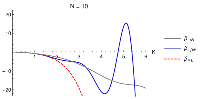
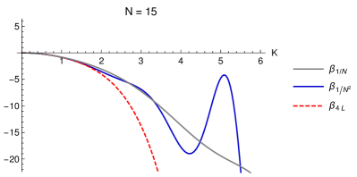
Figure 1: The $\beta$-function of Eq. (10) truncated to $\mathcal{O}(1/N)$, $\beta_{1/N}$, and to $\mathcal{O}(1/N^{2})$, $\beta_{1/N^{2}}$ along with the four-loop perturbative result, $\beta_{4\mathrm{L}}$, as a function of the rescaled coupling $K=gN$ for $N=10,15$.

We show the $\beta$-function of Eq. (10) truncated to $\mathcal{O}(1/N)$, $\beta_{1/N}$, and to $\mathcal{O}(1/N^{2})$, $\beta_{1/N^{2}}$, along with the four-loop perturbative result in Fig. 1 as a function of the rescaled coupling $K=gN$ for $N=10,15$. We conclude that there is no clear hint for the IR fixed point in the region where the perturbative series is under control.

To conclude the section, let us comment on the radius of convergence of the GN $\beta$-function at large $N$. The $\beta$-function does not have any singularities for positive couplings, although the resummed functions get contributions from graphs that grow polynomially with the loop order. Therefore, one expects to find a finite radius of convergence, similarly as in e.g. QED Palanques-Mestre and Pascual (1984). In the present case, the singularities do appear, but at negative coupling values so that the radius of convergence in the complex plane is indeed finite; this is related to the fact that the Wilson–Fisher fixed point exists above the critical dimension. For positive coupling values this translates to a regular, though wildly oscillatory, behaviour.

III Two-coupling case: Gross–Neveu–Yukawa model

III.1 Setup

The GNY model is the bosonised GN model with the scalar promoted to dynamical degree of freedom. It describes $N$ massless fermion flavours, $\psi$, coupling to a massless real scalar, $\phi$, via Yukawa interaction

$$\mathcal{L}_{\mathrm{GNY}}=\bar{\psi}\mathrm{i}\not{\partial}\psi-\frac{1}{2}\partial_{\mu}\phi\partial^{\mu}\phi+g_{1}\phi\bar{\psi}\psi+g_{2}\phi^{4}.$$ (17)

The critical dimension of the Yukawa interaction is ${d_{c}=4}$, and we will work in ${d=4-\epsilon}$ dimensions and $\overline{\mathrm{MS}}$ renormalisation scheme. We follow the notations of Refs Mihaila et al. (2017); Zerf et al. (2017) in order to provide for a straight-forward comparison with the perturbative result and define rescaled couplings

$$y\equiv\frac{g_{1}^{2}\mu^{\epsilon}}{8\pi^{2}},\quad K\equiv 2yN,\quad\text{and}\quad\lambda\equiv\frac{g_{2}\mu^{\epsilon}}{8\pi^{2}}.$$ (18)

III.2 The $\beta$-functions from the critical exponents

The critical exponents, $\omega_{\pm}$, for the GNY model were recently computed up to $1/N^{2}$ Gracey (2017); Manashov and Strohmaier (2018), and on the other hand, they are known perturbatively up to four-loop level Mihaila et al. (2017); Zerf et al. (2017). The computation for the Yukawa $\beta$-function using bubble-resummation method was carried out up to $\mathcal{O}(1/N)$ in Ref. Alanne and Blasi (2018a).

The Yukawa $\beta$-function at $\mathcal{O}(1/N)$ depends only on the Yukawa coupling, $y$:

$$\beta_{y}=(d-d_{c})y+y^{2}(2N+3+F_{1}(yN)).$$ (19)

Conversely, the $\beta$-function for the quartic coupling, $\lambda$, at $\mathcal{O}(1/N)$ is

$$\begin{split}\beta_{\lambda}=&(d-d_{c})\lambda+y^{2}(-N+F_{2}(yN))\\ &+\lambda^{2}(36+F_{3}(yN))+y\lambda(4N+F_{4}(yN)).\end{split}$$ (20)

According to Eqs (19) and (20), the coupled system of $\beta$-functions at $\mathcal{O}(1/N)$ contains four unknown functions, namely $F_{1}$, $F_{2}$, $F_{3}$ and $F_{4}$. Note that $F_{1-4}$ are functions of the rescaled Yukawa coupling only due to the $1/N$ counting. Diagrammatically this corresponds to chain of fermion bubbles. Similar diagrams of scalar bubbles lack the $N$ enhancement, and these chains are subleading.

We can constrain $F_{1-4}$ exploiting the knowledge of the critical exponents, $\omega_{\pm}$, by first determining the critical couplings such that $\beta_{y,\lambda}=0$. From the first equation, using $d-d_{c}=-\epsilon$, we find

$$y^{c}=\frac{\epsilon}{2N+3+F_{1}(y^{c}N)},$$ (21)

and from the second

$$\begin{split}\lambda^{c}=\ \frac{\epsilon-y^{c}\left(4N+F_{4}(y^{c}N)\right)+\sqrt{\Delta^{c}}}{2\left(36+F_{3}(y^{c}N)\right)}\end{split}$$ (22)

where we have taken the positive solution for $\lambda^{c}$ and defined

$$\begin{split}\Delta^{c}\equiv&\left[-\epsilon+y^{c}(4N+F_{4}(y^{c}N))\right]^{2}\\ &-4(36+F_{3}(y^{c}N))(y^{c})^{2}(-N+F_{2}(y^{c}N)).\end{split}$$ (23)

Up to leading order in $1/N$, we have

$$y^{c}=\frac{\epsilon}{2N}+\mathcal{O}(1/N^{2}),\quad\lambda^{c}=\frac{\epsilon}{4N}+\mathcal{O}(1/N^{2}).$$ (24)

Since $\frac{\partial\beta_{y}}{\partial\lambda}\equiv 0$, the eigenvalues of the Jacobian, $\omega_{\mp}$, directly correspond to $\frac{\partial\beta_{y}}{\partial y}$ and $\frac{\partial\beta_{\lambda}}{\partial\lambda}$ at criticality, respectively. Explicitly,

$$\frac{\partial\beta_{y}}{\partial y}=\epsilon+\frac{1}{4N}\epsilon^{2}F_{1}^{\prime}(\epsilon/2)=\epsilon+\frac{1}{N}\omega^{(1)}_{-}(4-\epsilon),$$ (25)

and

$$\frac{\partial\beta_{\lambda}}{\partial\lambda}= \epsilon+\frac{\epsilon}{2N}\left(30-2F_{1}(\epsilon/2)+F_{3}(\epsilon/2)+F_{4}(\epsilon/2)\right)$$

$$= \epsilon+\frac{1}{N}\tilde{\omega}^{(1)}_{+}(\epsilon).$$ (26)

For simplicity, we denote $\tilde{\omega}_{\pm}^{(1)}(\epsilon)\equiv\omega_{\pm}^{(1)}(4-\epsilon)$ in the following. Equation (25) yields

$$F_{1}(t)=\int_{0}^{t}\frac{\tilde{\omega}^{(1)}_{-}(2\epsilon)}{\epsilon^{2}}\text{d}\epsilon,$$ (27)

whereas Eq. (26) gives

$$30-2F_{1}(\epsilon/2)+F_{3}(\epsilon/2)+F_{4}(\epsilon/2)=2\frac{\tilde{\omega}^{(1)}_{+}(\epsilon)}{\epsilon}.$$ (28)

As we can see from Eq. (28), $\beta_{\lambda}$ cannot be computed with the knowledge of $\omega_{\pm}$, since only the combination $F_{3}+F_{4}$ can be accessed. In particular, $F_{2}$ is fully unconstrained. This shows that the critical exponents encoding the slope of the $\beta$-function can fully determine the $\beta$-function only for single-coupling theory, while for multi-coupling theory they are sensitive only to certain combinations. Therefore, either more information is input or one needs to rely on a direct computation to get $\beta_{\lambda}$ in a closed form.

Nevertheless, the knowledge of $\omega_{\pm}$ can be used to obtain independent cross-checks and gain information regarding the radius of convergence of the $1/N$ expansion. The explicit formulae for $\tilde{\omega}^{(1)}_{\mp}$ are Gracey (2017); Manashov and Strohmaier (2018)

$$\begin{split}\tilde{\omega}^{(1)}_{-}(t)&=-\frac{t\Gamma(4-t)}{\pi\Gamma\left(2-\frac{t}{2}\right)\Gamma\left(3-\frac{t}{2}\right)}\text{sin}\left(\frac{\pi t}{2}\right),\\ \vphantom{\frac{\frac{\frac{1}{2}}{\frac{1}{2}}}{\frac{1}{2}}}\tilde{\omega}^{(1)}_{+}(t)&=\frac{3t-10}{t}\tilde{\omega}^{(1)}_{-}(t).\end{split}$$ (29)

We show the critical exponents $\tilde{\omega}_{\pm}^{(1)}(t)$ along with the $\mathcal{O}(1/N^{2})$ results Manashov and Strohmaier (2018), $\tilde{\omega}_{\pm}^{(2)}(t)$, in Fig. 2. The $\mathcal{O}(1/N^{2})$ results indicate that there is a new singularity not present at $\mathcal{O}(1/N)$ occurring at $t=3$. Correspondingly, this would suggest a shrinking in the radius of convergence for the $\beta$-functions when higher orders are included. However, as we will show in the next sections, this singularity is actually already present at $\mathcal{O}(1/N)$, namely in the functions $F_{2},F_{3},F_{4}$, but is exactly cancelled in $\tilde{\omega}_{+}^{(1)}$, Eq. (28).

The connection between $\beta_{y,\lambda}$ and $\omega_{\mp}$ at $\mathcal{O}(1/N^{2})$ is enstablished in Appendix A. This allows us to derive conditions analogous to Eq. (28) for the new unknowns parametrizing the $\beta$-functions at $\mathcal{O}(1/N^{2})$.

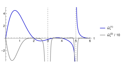
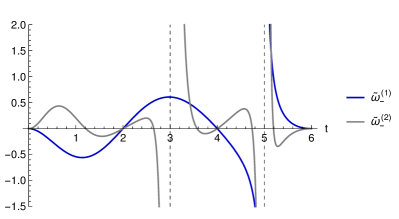
Figure 2: The first two coefficients of the $1/N$ expansion of the critical exponents $\tilde{\omega}_{\pm}=\sum_{n=1}^{\infty}\tilde{\omega}_{\pm}^{(n)}/N^{n}$. The explicit formulae for the $\mathcal{O}(1/N^{2})$ coeffiecients can be found in Ref. Manashov and Strohmaier (2018).

III.3 Bubble resummation

The knowledge of the critical exponent $\omega_{-}$ at $\mathcal{O}(1/N)$ is enough to obtain the explicit form of $\beta_{y}$ in Eq. (19) at the same order in $1/N$. This is not the case for $\beta_{\lambda}$ in Eq. (20), as the information contained in $\omega_{+}$ can only constrain a combinations of $F_{1}$, $F_{3}$ and $F_{4}$, see Eq. (28). In order to obtain $\beta_{\lambda}$ at the order $1/N$, we have thus to rely on explicit bubble resummation.

The $\beta$-function for $\lambda$ is obtained by acting with derivatives on the 1PI vertex counterterm, $Z_{\lambda}$, and on the scalar self-energy counterterm, $Z_{S}$. The bare coupling, $\lambda_{0}$, and the renormalized coupling, $\lambda$, are related via

$$\lambda_{0}=Z_{\lambda}Z_{S}^{-2}\lambda,$$ (30)

and the $\beta$-function is

$$\beta_{\lambda}=\lambda\left(\lambda\frac{\partial}{\partial\lambda}+K\frac{\partial}{\partial K}\right)\,\text{ln}\,\left(Z_{\lambda}Z_{S}^{-2}\right)_{1/\epsilon}.$$ (31)

The self-energy renormalisation constant, $Z_{S}$, has been computed in Ref. Alanne and Blasi (2018a) up to $\mathcal{O}(1/N)$, and reads:

$$Z_{S}=1-\frac{K}{\epsilon}-\frac{1}{\epsilon N}\int_{0}^{K}\left(\xi_{0}(t)-\xi_{0}(0)+\xi(t,1)K\right)\mathrm{d}t,$$ (32)

where

$$\xi_{0}(t)=-\frac{(1-t)\Gamma(4-t)}{\Gamma\left(2-\frac{t}{2}\right)\Gamma\left(3-\frac{t}{2}\right)\pi t}\sin\left(\frac{\pi t}{2}\right),$$ (33)

and

$$\xi(t,1)=\frac{1}{1-t}\xi_{0}(t).$$ (34)

The coupling-constant renormalisation constant, $Z_{\lambda}$, is given by

$$Z_{\lambda}=1-\text{div}\{Z_{\lambda}\Lambda_{0}(\lambda_{0},K_{0},p^{2},\epsilon)\},$$ (35)

where $K_{0}$ is the rescaled Yukawa coupling, and $\Lambda_{0}$ contains the 1PI contributions to the four-point function.

At the order $\mathcal{O}(1/N)$, we have

$$\begin{split}\Lambda_{0}=&\lambda_{0}\sum_{n=0}^{\infty}K_{0}^{n}\Lambda^{(n+1)}_{\lambda}(p^{2},\epsilon)+\frac{1}{\lambda_{0}N}K_{0}^{2}\Lambda_{K}^{(1)}(p^{2},\epsilon)\\ &+\frac{1}{\lambda_{0}N^{2}}K_{0}^{3}\sum_{n=0}^{\infty}K_{0}^{n}\Lambda_{K}^{(n+2)}(p^{2},\epsilon)\\ &+\frac{1}{N}K_{0}^{2}\sum_{n=0}^{\infty}K_{0}^{n}L^{(n+2)}(p^{2},\epsilon)\\ &+\frac{1}{\lambda_{0}N^{2}}K_{0}^{4}\sum_{n=0}^{\infty}K_{0}^{n}{\Lambda_{K}^{\prime}}^{(n+3)}(p^{2},\epsilon).\end{split}$$ (36)

The first term corresponds to a basic candy diagram where the Yukawa couplings only enter through the chain of fermion bubbles. The second term is the basic one-loop box diagram. The third term is a box diagram with an additional internal scalar propagator. The fourth term is a candy with two different vertices, namely one $\lambda$ and one effective quartic made of a fermion loop. The last term is a three-loop candy diagram with two fermion loops as effective quartics. The different topologies are shown in Figs 3–6.

The $p^{2}$ in the arguments refers generically to the IR regulator. We use two IR regulation strategies depending on the subclass of diagrams: For fermion-box type diagrams, we use a convenient choice of non-zero external momenta, and for the scalar-candy-type diagrams we give a non-zero regulating mass for the propagating scalars. The sum of the contributions in each of these subclasses is IR finite, justifying the different regularisations.

After trading the bare couplings with the renormalized couplings,

$$\lambda_{0}=Z_{\lambda}Z_{S}^{-2}\lambda,\quad K_{0}=Z_{S}^{-1}(Z_{V}Z_{F}^{-1})^{2}K,$$ (37)

where $Z_{V,F}=1+\mathcal{O}(1/N)$ are the renormalisation constants for the 1PI Yukawa vertex and fermion self-energy, resp., and keeping only term that contribute up to $\mathcal{O}(1/N)$, we find for $Z_{\lambda}$:

$$Z_{\lambda}=1 -\text{div}\bigg{\{}\lambda Z_{S}^{-2}\sum_{n=0}^{\infty}(Z_{S}^{-1}K)^{n}\Lambda_{\lambda}^{(n+1)}$$

$$+\frac{1}{N}K^{2}Z_{S}^{-2}\sum_{n=0}^{\infty}(Z_{S}^{-1}K)^{n}\left(L^{(n+2)}-2D\Lambda_{\lambda}^{(n+1)}\right)$$

$$+\frac{1}{\lambda N}K^{2}(Z_{V}Z_{F}^{-1})^{4}\Lambda_{K}^{(1)}$$

$$+\frac{1}{\lambda N^{2}}K^{3}Z_{S}^{-1}\sum_{n=0}^{\infty}(Z_{S}^{-1}K)^{n}\Lambda_{K}^{(n+2)}$$ (38)

$$+\frac{1}{\lambda N^{2}}K^{4}Z_{S}^{-2}\sum_{n=0}^{\infty}(Z_{S}^{-1}K)^{n}\left(D^{2}{\Lambda_{\lambda}}^{(n+1)}\right.$$

$$\left.\qquad\qquad-D{L}^{(n+2)}+{\Lambda_{K}^{\prime}}^{(n+3)}\right)\bigg{\}},$$

where we have iterated Eq. (35) to include all the contributions up to $\mathcal{O}(1/N)$, and we have defined $D$ as

$$D=\text{div}\{\Lambda_{K}^{(1)}\}.$$ (39)

Notice that, despite the explicit $1/N^{2}$ dependence, the $1/\lambda N^{2}$ contributions are actually $\mathcal{O}(1/N)$ when interpreted in terms of the rescaled quartic, $\lambda N$.

After taking derivatives according to Eq. (31), the first line in Eq. (III.3) will give the $\lambda^{2}$-contribution in Eq. (20), namely the function $F_{3}$, and the second line will contribute to $F_{4}$. The last four lines behave like $1/\lambda$ and correspond to the pure Yukawa contribution, $F_{2}$.

III.4 $F_{3}$, $F_{4}$ and cross-check

We compute here $F_{3}$ and $F_{4}$ by explicit resummation and cross-check our result with Eq. (28). Diagrammatically, $F_{3}$ corresponds to Fig. 3, where the internal scalar lines are dressed with fermion bubbles.

Figure 3: Diagram for $F_{3}(yN)$. The gray blob represents a bubble chain.

To obtain its expression, we refer to the first line of Eq. (III.3) and compute:

$$T_{3}\equiv- \text{div}\left\{\lambda Z_{S}^{-2}\sum_{n=0}^{\infty}(Z_{S}^{-1}K)^{n}\Lambda_{\lambda}^{(n+1)}\right\}$$ (40)

$$=- \text{div}\left\{\lambda\sum_{n=0}^{\infty}K^{n}\sum_{i=0}^{n}\left(\begin{array}[]{c}n+1\\ i\end{array}\right)\frac{(-1)^{i}}{\epsilon^{i}}\Lambda_{\lambda}^{(n-i+1)}\right\}.$$ (43)

The function $\Lambda_{\lambda}^{(m)}$ is found to be

$$\Lambda_{\lambda}^{(m)}=\frac{1}{\epsilon^{m}}l(\epsilon,m)=\frac{1}{\epsilon^{m}}\sum_{j=0}^{\infty}(m\epsilon)^{j}l_{j}(\epsilon).$$ (44)

After resummation, and keeping only the $1/\epsilon$ pole of $T_{3}$, we find

$$T_{3}=-\frac{1}{\epsilon}\lambda\,l_{0}(K)\ +\dots\,,$$ (45)

where

$$l_{0}(t)=\frac{9\cdot 2^{4-t}\Gamma\left(\frac{3}{2}-\frac{t}{2}\right)\text{sin}\left(\frac{\pi t}{2}\right)}{\pi^{3/2}t\Gamma\left(2-\frac{t}{2}\right)}.$$ (46)

By adopting the same convention of Eq. (20), the function $F_{3}$ is

$$F_{3}(t)=l_{0}(2t)+2tl_{0}^{\prime}(2t)-36,$$ (47)

where $-36$ removes the one-loop contribution.

To compute $F_{4}$, we start from the second line of Eq. (III.3), which diagrammatically corresponds to Fig. 4:

Figure 4: Diagram for $F_{4}(yN)$. The gray blob represents a chain of fermion bubbles. The labels $N$ and $T$ correspond to non-twisted and twisted fermion bubbles, respectively, and are pictorially represented below the $F_{4}$ diagram.

$$T_{4}\equiv-\frac{K^{2}}{N}\text{div}\left\{Z_{S}^{-2}\sum_{n=0}^{\infty}(Z_{S}^{-1}K)^{n}\left(L^{(n+2)}-2D\Lambda_{\lambda}^{(n+1)}\right)\right\}$$

$$=-\frac{K^{2}}{N}\text{div}\left\{\sum_{n=0}^{\infty}K^{n}\sum_{i=0}^{n}\left(\begin{array}[]{c}n+1\\ i\end{array}\right)\frac{(-1)^{i}}{\epsilon^{i}}\Gamma(n+2-i,\epsilon)\right\}$$ (50)

where we have introduced

$$\Gamma(m,\epsilon)\equiv L^{(m)}-2D\Lambda_{\lambda}^{(m-1)}=\frac{1}{m\epsilon^{m}}(-1)^{m}\gamma(\epsilon,m),$$ (51)

with

$$\gamma(\epsilon,m)=\sum_{j=0}^{\infty}(m\epsilon)^{j}\gamma_{j}(\epsilon).$$ (52)

After resummation, and keeping only the $1/\epsilon$ pole of $T_{4}$, we find

$$T_{4}=\frac{1}{\epsilon N}\left(K\gamma(K,1)-\int_{0}^{K}\gamma_{0}(t)\text{d}t\right)+\dots\,,$$ (53)

where

$$\gamma_{0}(t)=\frac{3\cdot 2^{3-t}(t-3)\Gamma\left(\frac{3}{2}-\frac{t}{2}\right)}{\pi^{3/2}t\Gamma(2-t/2)}\text{sin}\left(\frac{\pi t}{2}\right),$$ (54)

and

$$\gamma(t,1)=\frac{1}{1-t/3}\gamma_{0}(t).$$ (55)

Figure 5: Different types of box diagrams for $F_{2}(yN)$. The gray blob represents a chain of fermion bubbles.

Besides $T_{4}$, the function $F_{4}$ gets contribution from $Z_{S}$ in Eq. (32). Altogether, in the convention of Eq. (20), it is given by

$$F_{4}(t)= \,2\gamma(2t,1)-2\gamma_{0}(2t)+4t\gamma^{\prime}(2t,1)$$ (56)

$$+4\xi_{0}(2t)+8t\xi(2t,1)+6+4\int_{0}^{2t}\xi(x,1)\text{d}x.$$

With the results of Eqs (47) and (56) together with Eq. (27), one can check that Eq. (28) is fulfilled. This provides a powerful cross-check for our computation.

III.5 The function $F_{2}$

The function $F_{2}$ can be computed evaluating the $1/\lambda$ terms in the last four lines of Eq. (III.3), corresponding to the one-loop box diagram, the box diagrams with additional internal scalar propagator in Fig. 5 and to the candy diagrams in Fig. 6.

Let us start with the box contribution. The counterterms $Z_{V}$ and $Z_{F}$ have been computed up to $\mathcal{O}(1/N)$ in Ref. Alanne and Blasi (2018a) and read:

$$\begin{split}&Z_{V}=1+\frac{1}{2N}\sum_{n=1}^{\infty}\frac{K^{n}}{\epsilon^{n}}\frac{v_{0}(\epsilon)}{n}\\ &Z_{F}=1-\frac{1}{4N}\sum_{n=1}^{\infty}\frac{K^{n}}{\epsilon^{n}}\frac{\sigma_{0}(\epsilon)}{n}.\end{split}$$ (57)

The third line in Eq. (III.3) gives a divergent part

$$T_{b_{1}}\equiv\frac{4K^{2}}{\lambda N}\left[\frac{D}{4}+\text{div}\left\{(\tilde{Z}_{F}-\tilde{Z}_{V})\Lambda_{F}^{(1)}(p^{2},\epsilon)\right\}\right],$$ (58)

where $\tilde{Z}_{F,V}\equiv Z_{F,V}-1$, and we have defined the finite part of the one-loop box diagram as

$$\Lambda_{F}^{(1)}=\Lambda^{(1)}_{K}-D.$$ (59)

The first term in Eq. (58) gives the basic one-loop contribution of the box diagram and will be omitted in the following. Using Eq. (57) and keeping only the $1/\epsilon$ pole of $T_{b_{1}}$, we have:

$$T_{b_{1}}=\frac{K^{2}}{\epsilon\lambda N^{2}}\int_{0}^{K}\Lambda_{F}^{(1)}(p^{2},t)(\sigma_{0}(t)+2v_{0}(t))\mathrm{d}t\ +\dots$$ (60)

As for the fourth line in Eq. (III.3), we have

$$T_{b_{2}}\equiv\frac{K^{3}}{\lambda N^{2}}\sum_{n=0}^{\infty}K^{n}\text{div}\sum_{i=0}^{n}\left\{\left(\begin{array}[]{c}n\\ i\end{array}\right)\frac{1}{\epsilon^{i}}\Lambda^{(n+2-i)}_{K}(p^{2},\epsilon)\right\}.$$ (61)

The quantity $\Lambda^{(m)}_{K}$ allows for the following expansion:

$$\Lambda^{(m)}_{K}(p^{2},\epsilon)=\frac{1}{\epsilon^{m}m(m-1)}\lambda(p^{2},\epsilon,m),$$ (62)

where $\lambda(p^{2},\epsilon,m)$ is regular for $\epsilon\rightarrow 0$ and can be written as

$$\lambda(m,\epsilon)=\sum_{j=0}^{\infty}(m\epsilon)^{j}\lambda_{j}(p^{2},\epsilon).$$ (63)

Plugging Eqs (62) and (63) in Eq. (61) and using the usual summation formulas, we find for the $1/\epsilon$ pole:

$$\begin{split}T_{b_{2}}=\frac{K}{\epsilon\lambda N^{2}}&\int_{0}^{K}\left(\vphantom{\frac{1}{2}}\lambda_{0}(t)-\lambda_{0}(0)\right.\\ &\left.\qquad\ +K\frac{\lambda(p^{2},t,1)-\lambda_{0}(t)}{t}\right)\text{d}t\ +\dots\end{split}$$ (64)

When the $1/\epsilon$ poles of $T_{b_{1}}$ and $T_{b_{2}}$ are put together, the $p^{2}$ dependence of $\lambda(p^{2},t,1)$ cancels. We find the $1/\epsilon$ pole of $Z_{\lambda}^{\text{box}}$ to be

$$\begin{split}Z_{\lambda}^{\text{box}}&=-(T_{b_{1}}+T_{b_{2}})\\ &=-\frac{K}{\epsilon\lambda N^{2}}\int_{0}^{K}\left(\vphantom{\frac{1}{2}}\lambda_{0}(t)-\lambda_{0}(0)\right.\\ &\left.\qquad\qquad\qquad\quad+K\frac{5-t}{4-5t+t^{2}}\lambda_{0}(t)\right)\text{d}t,\end{split}$$ (65)

where the function $\lambda_{0}(t)$ is given by

$$\lambda_{0}(t)=(t-1)\frac{\Gamma(4-t)\,\text{sin}\left(\frac{\pi t}{2}\right)}{\pi t\Gamma\left(2-\frac{t}{2}\right)^{2}}.$$ (66)

In the convention of Eq. (20),

$$\begin{split}F_{2}^{\text{box}}(t)=&\int_{0}^{2t}\frac{x-5}{x^{2}-5x+4}\lambda_{0}(x)\text{d}x\\ &+\lambda_{0}(0)-\frac{4}{4-10t+4t^{2}}\lambda_{0}(2t).\end{split}$$ (67)

Let us now compute the contribution of the candy diagrams in Fig. 6, $Z_{\lambda}^{\text{candy}}$, arising from the last two lines of Eq. (III.3). It can be rewritten as

$$~{}T_{c}\equiv\frac{K^{4}}{\lambda N^{2}}\mathrm{div}\left\{\sum_{n=0}^{\infty}K^{n}\sum_{i=0}^{n}\left(\begin{array}[]{c}n+1\\ i\end{array}\right)\frac{1}{\epsilon^{i}}C^{(n+1-i)}\right\},$$ (68)

where

$$C^{(n+1-i)}\equiv D^{2}{\Lambda_{\lambda}}^{(n+1-i)}-D{L}^{(n+2-i)}+{\Lambda_{K}^{\prime\,(n+3-i)}}.$$ (69)

Figure 6: Candy diagrams for $F_{2}(yN)$. The basic diagram is the three-loop diagram $\Lambda^{\prime}_{K}$. The fermion loops $A,B$ are either of the form $N$ (non-twisted) or $T$ (twisted), cf. Fig. 4. The diagrams $DL$ and $D^{2}\Lambda_{\lambda}$ come from $\Lambda^{\prime}_{K}$ when $A$ or $B$ are shrunk to a counterterm vertex $D$, which is the same for $N$ and $T$.

The structure of $C^{(m)}$ is:

$$C^{(m)}=\frac{1}{\epsilon^{m+2}}\frac{1}{(m+1)(m+2)}c(p^{2},\epsilon,m),$$ (70)

where the function $c(p^{2},\epsilon,m)$ is regular for $\epsilon\rightarrow 0$ and can be expanded as

$$c(p^{2},\epsilon,m)=\sum_{j=0}^{\infty}(m\epsilon)^{j}c_{j}(p^{2},\epsilon).$$ (71)

The IR regulator, $p^{2}$, stands here for a soft mass for the scalar field. Plugging Eqs (70) and (71) in Eq. (68) yields

$$T_{c}=\frac{K^{4}}{\lambda N^{2}}\mathrm{div}\left\{\sum_{n=0}^{\infty}\frac{K^{n}}{\epsilon^{n+3}}\sum_{j=0}^{n+2}\epsilon^{j}c_{j}(p^{2},\epsilon)S(n,j)\right\},$$ (72)

where

$$S(n,j)=\sum_{i=0}^{n}\left(\begin{array}[]{c}n+1\\ i\end{array}\right)(-1)^{i}\frac{(n+2-i)^{j-1}}{n+3-i}.$$ (73)

We find

$$S(n,j)=\begin{cases}(-1)^{n}\frac{n+1}{2(n+3)}\quad&j=0,\\ (-1)^{n}\frac{(n+1)(n+4)}{2(n+2)(n+3)}&j\,\text{odd},\\ (-1)^{n}\frac{8+n(n+5)}{2(n+2)(n+3)}&j\,\text{even}.\end{cases}$$ (74)

Eq. (74) tells that three functions are relevant: $c_{0}(\epsilon)$, $c_{e}(\epsilon)$, and $c_{o}(\epsilon)$,

$$c_{e}(\epsilon) \equiv\sum_{j\,\text{even}}^{\infty}\epsilon^{j}c_{j}(\epsilon)=\frac{c(p^{2},\epsilon,1)+c(p^{2},\epsilon,-1)}{2}-c_{0}(\epsilon),$$

(75)

$$c_{o}(\epsilon) \equiv\sum_{j\,\text{odd}}^{\infty}\epsilon^{j}c_{j}(\epsilon)=\frac{c(p^{2},\epsilon,1)-c(p^{2},\epsilon,-1)}{2},$$

where the summation over $j$ has been extended to $\infty$ without affecting the result (namely, finite terms in the $\epsilon\rightarrow 0$ limit), and all the resulting functions are found to be independent of the IR regulator. They read

$$c_{0}(t)= -3\frac{2^{4-t}\,\Gamma\left(\frac{5}{2}-\frac{t}{2}\right)\text{sin}\left(\frac{\pi t}{2}\right)}{\pi^{3/2}t\Gamma\left(2-\frac{t}{2}\right)},$$ (76)

$$c_{e}(t)= \frac{t^{2}}{6(3-t)}c_{0}(t),$$ (77)

$$c_{o}(t)= \frac{t(6-t)}{6(3-t)}c_{0}(t).$$ (78)

After performing the sum over $n$ using Eqs (74)–(78), and retaining only the $1/\epsilon$ pole, we arrive at

$$T_{c}=\frac{1}{\epsilon\lambda N^{2}} \bigg{(}\frac{1}{2}K^{2}\left(c_{0}(K)+c_{0}(0)\right)+\frac{K^{3}}{6-2K}c_{0}(K)$$

$$+\frac{1}{3}K\int_{0}^{K}(t-3-K)c_{0}(t)\text{d}t\bigg{)}\ +\dots$$ (79)

In the convention of Eq. (20),

$$F_{2}^{\text{candy}}(t)= \,\frac{9-24t+8t^{2}}{2(2t-3)^{2}}c_{0}(2t)+\frac{3t}{2t-3}c_{0}^{\prime}(2t)$$

$$-\frac{1}{6}\left(3c_{0}(0)-2\int_{0}^{2t}c_{0}(x)\text{d}x\right).$$ (80)

Combining Eqs (67) and (III.5), the function $F_{2}(t)$ is then

$$F_{2}(t)=F_{2}^{\text{box}}(t)+F_{2}^{\text{candy}}(t).$$ (81)

We show the functions $F_{1}$, $F_{2}$, $F_{3}$ and $F_{4}$ in Fig. 7. In particular, we notice that functions $F_{2-4}$ feature the first singularity at $t=3/2$, which is not present in the $\mathcal{O}(1/N)$ critical exponents but shows up at the $\mathcal{O}(1/N^{2})$ level. This singularity gets exactly cancelled in the combination of $F_{3}$ and $F_{4}$ entering $\tilde{\omega}_{+}^{(1)}$, Eq. (28), while $F_{2}$ does not contribute to $\omega_{\pm}^{(1)}$.

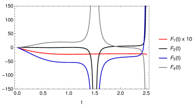
Figure 7: The functions $F_{1}$, $F_{2}$, $F_{3}$ and $F_{4}$ given in Eqs (25), (81), (47), (47), resp. $F_{1}$ has the first (logarithmic) singularity at $t=5/2$, whereas $F_{2-4}$ show a second-order pole at $t=3/2$.

III.6 Perturbative results

We provide here the expansion of the functions $F_{1-4}$ in order to check against the known perturbative results and predict the $\mathcal{O}(1/N)$ terms that would appear up to six-loop order.

In the following, we give the explicit term-by-term expansions of the $\beta$-functions, given in Eqs (19) and (20). First, for the Yukawa $\beta$-function we have

$$y^{2}F_{1}(yN)= -6y^{3}N+\frac{7}{2}y^{4}N^{2}+\frac{11}{6}y^{5}N^{3}$$

$$+\left(\frac{19}{16}-3\zeta_{3}\right)y^{6}N^{4}$$ (82)

$$+\left(\frac{7}{8}+\frac{14}{5}\zeta_{3}-\frac{18}{5}\zeta_{4}\right)y^{7}N^{5}+\mathcal{O}(y^{8}).$$

As for the quartic-coupling $\beta$-function, Eq. (20), one can predict the coefficients based on $F_{2}$, $F_{3}$ and $F_{4}$. Their contribution to the $\beta$-function is:

$$y^{2}F_{2}(yN) =4y^{3}N-\frac{157}{8}y^{4}N^{2}+\left(42\zeta_{3}-\frac{193}{6}\right)y^{5}N^{3}$$

$$\ +\left(-\frac{2623}{64}-\frac{157}{4}\zeta_{3}+90\zeta_{4}\right)y^{6}N^{4}$$ (83)

$$\ +\left(-\frac{3993}{80}-\frac{491}{5}\zeta_{3}-\frac{426}{5}\zeta_{4}+234\zeta_{5}\right)y^{7}N^{5}$$

$$\ +\mathcal{O}(y^{8}),$$

$$\begin{split}\lambda^{2}F_{3}(yN)=&-72y\lambda^{2}N-108y^{2}\lambda^{2}N^{2}\\ &+144(2\zeta_{3}-1)\lambda^{2}y^{3}N^{3}\\ &-180(1+2\zeta_{3}-3\zeta_{4})\lambda^{2}y^{4}N^{4}\\ &-216(1+2\zeta_{3}+3\zeta_{4}-6\zeta_{5})\lambda^{2}y^{5}N^{5}\\ &+\mathcal{O}(\lambda^{2}y^{6}),\end{split}$$ (84)

$$y\lambda F_{4} (yN)=7\lambda y^{2}N+\frac{217}{2}\lambda y^{3}N^{2}$$

$$\ +\left(\frac{1685}{12}-228\zeta_{3}\right)\lambda y^{4}N^{3}$$ (85)

$$\ +\left(\frac{699}{4}+248\zeta_{3}-450\zeta_{4}\right)\lambda y^{5}N^{4}$$

$$\ +\left(\frac{3359}{16}+\frac{2123}{5}\zeta_{3}+\frac{2409}{5}\zeta_{4}-1116\zeta_{5}\vphantom{\frac{1}{2}}\right)\lambda y^{6}N^{5}$$

$$\ +\mathcal{O}(\lambda y^{7}).$$

We have checked that the expansions up to $\mathcal{O}(N^{3})$ agree with the known leading-$N$ four-loop perturbative result Zerf et al. (2017). The $\mathcal{O}(N^{4})$ and $\mathcal{O}(N^{5})$ terms are the leading-$N$ prediction for the five- and six-loop terms, respectively.

IV Conclusions

Our goal in this paper was to compare the critical-point and bubble-resummation methods for computing the $\beta$-functions in the large-$N$ limit. While for the single-coupling theories, the methods are equivalent, we have shown that in the multi-coupling case the critical exponents are only sensitive to specific combinations of the different functions entering the $\beta$-functions, and direct computations by means of bubble resummations or additional information are needed to decipher this missing information. On the other hand, the critical-point method is more powerful for obtaining results beyond the leading $1/N$ order, and thereby the two methods can provide complementary information.

However, we envisage that it might be possible to reconstruct the full system of RG functions in a multiple-coupling theory within the critical-point formalism through extraction of the operator-product-expansion (OPE) coefficients. A detailed study of the three-point function Schwinger–Dyson equation would be necessary, from which one could extract the OPE consistently at every order in $1/N$ in a similar fashion as for the critical exponents. This is in line with the recent analyses carried out in the functional-RG framework Codello et al. (2017, 2018, 2019a, 2019b).

Concretely, we have presently computed the $\beta$-function for the quartic coupling in the GNY model, thereby completing the computation of the full system at $\mathcal{O}(1/N)$ level. While the critical exponents $\omega_{\pm}$ computed recently up to $\mathcal{O}(1/N^{2})$ imply that the radius of convergence of the critical exponents shrinks from $\mathcal{O}(1/N)$ to $\mathcal{O}(1/N^{2})$, our present result shows that this new pole only appearing in $\omega_{\pm}^{(2)}$ is actually already present at the $\mathcal{O}(1/N)$ level, when the full system of $\beta$-functions is known. We showed that the disappearance of the pole is due to a subtle cancellation between the various resummed function in the computation of the critical exponents.

For the one-coupling case we have briefly revisited the question about the possible IR fixed point of the two-dimensional GN model by studying the $\mathcal{O}(1/N^{2})$ $\beta$-function. This complements the previous studies using the four-loop perturbative results with the help of Padé approximants. We restate that there is no indication of an IR fixed point.

Appendix A Gross–Neveu–Yukawa $\beta$-functions at $1/N^{2}$

The $\mathcal{O}(1/N)$ ansatz for the GNY $\beta$-functions in Eqs (19) and (20) is extended to $\mathcal{O}(1/N^{2})$ as

$$\begin{split}\beta_{y}=&-\epsilon y+y^{2}[2N+3+F_{1}(yN)-y(9/8+F_{5}(yN))]\\ &-y^{2}\lambda(24+F_{6}(yN))+y\lambda^{2}(24+F_{7}(yN)),\end{split}$$ (86)

$$\begin{split}\beta_{\lambda}=&-\epsilon\lambda+y^{2}[-N+F_{2}(yN)+yF_{8}(yN)+\lambda F_{9}(yN)]\\ &+\lambda^{2}[36+F_{3}(yN)-\lambda(816+F_{11}(yN))]\\ &+y\lambda[4N+F_{4}(yN)+\lambda F_{10}(yN)],\end{split}$$ (87)

where we have introduced seven new unknown functions, $F_{5-11}$, such that $F_{5-11}(0)=0$. We then compute the Jacobian for $(\beta_{y},\beta_{\lambda})$ and we evaluate it at the Wilson–Fisher fixed point. The eigenvalues are then matched with the critical exponents $\omega_{\pm}$. At $\mathcal{O}(1/N^{2})$, we find the following relations:

$$\begin{split}&-57-4\left[3+F_{1}\left(\epsilon\right)\right]\left[2F_{1}^{\prime}\left(\epsilon\right)+\epsilon F_{1}^{\prime\prime}\left(\epsilon\right)\right]\\ &-8F_{5}\left(\epsilon\right)-2F_{7}\left(\epsilon\right)-8\epsilon F_{5}^{\prime}\left(\epsilon\right)\\ &-4\epsilon F_{6}^{\prime}\left(\epsilon\right)+2\epsilon F_{7}^{\prime}\left(\epsilon\right)=8\frac{\tilde{\omega}_{-}^{(2)}(2\epsilon)}{\epsilon^{2}}.\end{split}$$ (88)

and

$$-2520-4782\epsilon+8\epsilon F_{10}(\epsilon)-6\epsilon F_{11}(\epsilon)-288F_{2}(\epsilon)$$

$$-144F_{3}(\epsilon)-8F_{2}(\epsilon)F_{3}(\epsilon)-2F_{3}(\epsilon)^{2}-156F_{4}(\epsilon)$$

$$-4F_{3}(\epsilon)F_{4}(\epsilon)+16\epsilon F_{5}(\epsilon)+8\epsilon F_{6}(\epsilon)-4\epsilon F_{7}(\epsilon)$$

$$+8\epsilon F_{9}(\epsilon)-12\epsilon F_{3}^{\prime}(\epsilon)-12\epsilon F_{4}^{\prime}(\epsilon)+48F_{1}(\epsilon)$$ (89)

$$+24\epsilon F_{1}^{\prime}(\epsilon)+8F_{1}(\epsilon)^{2}-4F_{1}(\epsilon)F_{4}(\epsilon)+8\epsilon F_{1}(\epsilon)F_{1}^{\prime}(\epsilon)$$

$$-4\epsilon F_{1}(\epsilon)F_{3}^{\prime}(\epsilon)-4\epsilon F_{1}(\epsilon)F_{4}^{\prime}(\epsilon)=8\frac{\tilde{\omega}_{+}^{(2)}\left(2\epsilon\right)}{\epsilon}.$$

Clearly, one needs more input than $\omega_{\mp}^{(2)}$ to obtain $F_{5-11}$. On the other hand, direct computation at $\mathcal{O}(1/N^{2})$ is technically challenging and beyond the scope of this paper.

References

- Espriu et al. (1982) D. Espriu, A. Palanques-Mestre, P. Pascual, and R. Tarrach, Z. Phys. C13, 153 (1982).
- Palanques-Mestre and Pascual (1984) A. Palanques-Mestre and P. Pascual, Commun. Math. Phys. 95, 277 (1984).
- Kowalska and Sessolo (2018) K. Kowalska and E. M. Sessolo, JHEP 04, 027 (2018), arXiv:1712.06859 [hep-ph] .
- Antipin et al. (2018) O. Antipin, N. A. Dondi, F. Sannino, A. E. Thomsen, and Z.-W. Wang, Phys. Rev. D98, 016003 (2018), arXiv:1803.09770 [hep-ph] .
- Alanne and Blasi (2018a) T. Alanne and S. Blasi, JHEP 08, 081 (2018a), [Erratum: JHEP09,165(2018)], arXiv:1806.06954 [hep-ph] .
- Alanne and Blasi (2018b) T. Alanne and S. Blasi, Phys. Rev. D98, 116004 (2018b), arXiv:1808.03252 [hep-ph] .
- Vasiliev et al. (1981a) A. N. Vasiliev, Yu. M. Pismak, and Yu. R. Khonkonen, Theor. Math. Phys. 46, 104 (1981a), [Teor. Mat. Fiz.46,157(1981)].
- Vasiliev et al. (1981b) A. N. Vasiliev, Yu. M. Pismak, and Yu. R. Khonkonen, Theor. Math. Phys. 47, 465 (1981b), [Teor. Mat. Fiz.47,291(1981)].
- Vasiliev et al. (1982) A. N. Vasiliev, Yu. M. Pismak, and Yu. R. Khonkonen, Theor. Math. Phys. 50, 127 (1982), [Teor. Mat. Fiz.50,195(1982)].
- Gracey (1993) J. A. Gracey, Phys. Lett. B318, 177 (1993), arXiv:hep-th/9310063 [hep-th] .
- Gracey (1996) J. A. Gracey, Phys. Lett. B373, 178 (1996), arXiv:hep-ph/9602214 [hep-ph] .
- Ciuchini et al. (2000) M. Ciuchini, S. E. Derkachov, J. A. Gracey, and A. N. Manashov, Nucl. Phys. B579, 56 (2000), arXiv:hep-ph/9912221 [hep-ph] .
- Gracey (1991) J. A. Gracey, Int. J. Mod. Phys. A6, 395 (1991), [Erratum: Int. J. Mod. Phys.A6,2755(1991)].
- Gracey (1992) J. A. Gracey, Phys. Lett. B297, 293 (1992).
- Derkachov et al. (1993) S. E. Derkachov, N. A. Kivel, A. S. Stepanenko, and A. N. Vasiliev, (1993), arXiv:hep-th/9302034 [hep-th] .
- Vasiliev et al. (1993) A. N. Vasiliev, S. E. Derkachov, N. A. Kivel, and A. S. Stepanenko, Theor. Math. Phys. 94, 127 (1993), [Teor. Mat. Fiz.94,179(1993)].
- Vasiliev and Stepanenko (1993) A. N. Vasiliev and A. S. Stepanenko, Theor. Math. Phys. 97, 1349 (1993), [Teor. Mat. Fiz.97,364(1993)].
- Gracey (1994a) J. A. Gracey, Int. J. Mod. Phys. A9, 567 (1994a), arXiv:hep-th/9306106 [hep-th] .
- Gracey (1994b) J. A. Gracey, Int. J. Mod. Phys. A9, 727 (1994b), arXiv:hep-th/9306107 [hep-th] .
- Gracey (2017) J. A. Gracey, Phys. Rev. D96, 065015 (2017), arXiv:1707.05275 [hep-th] .
- Manashov and Strohmaier (2018) A. N. Manashov and M. Strohmaier, Eur. Phys. J. C78, 454 (2018), arXiv:1711.02493 [hep-th] .
- Gracey (2019) J. A. Gracey, Int. J. Mod. Phys. A33, 1830032 (2019), arXiv:1812.05368 [hep-th] .
- Ryttov and Tuominen (2019) T. A. Ryttov and K. Tuominen, (2019), arXiv:1903.09089 [hep-th] .
- Dondi et al. (2019) N. A. Dondi, G. V. Dunne, M. Reichert, and F. Sannino, (2019), arXiv:1903.02568 [hep-th] .
- Antipin et al. (2019) O. Antipin, N. A. Dondi, F. Sannino, and A. E. Thomsen, Phys. Rev. D99, 025004 (2019), arXiv:1808.00482 [hep-th] .
- Ferreira and Gracey (1998) P. M. Ferreira and J. A. Gracey, Nucl. Phys. B525, 435 (1998), arXiv:hep-th/9712138 [hep-th] .
- Friess and Gubser (2006) J. J. Friess and S. S. Gubser, Nucl. Phys. B750, 111 (2006), arXiv:hep-th/0512355 [hep-th] .
- Schonfeld (1975) J. F. Schonfeld, Nucl. Phys. B95, 148 (1975).
- Choi et al. (2017) G. Choi, T. A. Ryttov, and R. Shrock, Phys. Rev. D95, 025012 (2017), arXiv:1612.05580 [hep-th] .
- Gracey et al. (2016) J. A. Gracey, T. Luthe, and Y. Schroder, Phys. Rev. D94, 125028 (2016), arXiv:1609.05071 [hep-th] .
- Thirring (1958) W. E. Thirring, Annals Phys. 3, 91 (1958), [,509(1958)].
- Mueller and Trueman (1971) A. H. Mueller and T. L. Trueman, Phys. Rev. D4, 1635 (1971).
- Gomes and Lowenstein (1972) M. Gomes and J. H. Lowenstein, Nucl. Phys. B45, 252 (1972).
- Shrock (2014) R. Shrock, Phys. Rev. D89, 045019 (2014), arXiv:1311.5268 [hep-th] .
- Mihaila et al. (2017) L. N. Mihaila, N. Zerf, B. Ihrig, I. F. Herbut, and M. M. Scherer, Phys. Rev. B96, 165133 (2017), arXiv:1703.08801 [cond-mat.str-el] .
- Zerf et al. (2017) N. Zerf, L. N. Mihaila, P. Marquard, I. F. Herbut, and M. M. Scherer, Phys. Rev. D96, 096010 (2017), arXiv:1709.05057 [hep-th] .
- Codello et al. (2017) A. Codello, M. Safari, G. P. Vacca, and O. Zanusso, JHEP 04, 127 (2017), arXiv:1703.04830 [hep-th] .
- Codello et al. (2018) A. Codello, M. Safari, G. P. Vacca, and O. Zanusso, Eur. Phys. J. C78, 30 (2018), arXiv:1705.05558 [hep-th] .
- Codello et al. (2019a) A. Codello, M. Safari, G. P. Vacca, and O. Zanusso, Eur. Phys. J. C79, 331 (2019a), arXiv:1809.05071 [hep-th] .
- Codello et al. (2019b) A. Codello, M. Safari, G. P. Vacca, and O. Zanusso (2019) arXiv:1905.01086 [hep-th] .