A Kaczmarz Algorithm for Solving Tree Based Distributed Systems of Equations
Abstract.
The Kaczmarz algorithm is an iterative method for solving systems of linear equations. We introduce a modified Kaczmarz algorithm for solving systems of linear equations in a distributed environment, i.e. the equations within the system are distributed over multiple nodes within a network. The modification we introduce is designed for a network with a tree structure that allows for passage of solution estimates between the nodes in the network. We prove that the modified algorithm converges under no additional assumptions on the equations. We demonstrate that the algorithm converges to the solution, or the solution of minimal norm, when the system is consistent. We also demonstrate that in the case of an inconsistent system of equations, the modified relaxed Kaczmarz algorithm converges to a weighted least squares solution as the relaxation parameter approaches .
Key words and phrases:
Kaczmarz method, linear equations, least squares, distributed optimization2000 Mathematics Subject Classification:
Primary: 65F10, 15A06; Secondary 68W15, 41A651. Introduction
The Kaczmarz method ([11], 1937) is an iterative algorithm for solving a system of linear equations , where is an matrix. Written out, the equations are for , where is the th row of the matrix , and we take the dot product to be linear in both variables. Given a solution guess and an equation number , we calculate (the residual for equation ), and define
| (1) |
This makes the residual of in equation equal to 0. Here and elsewhere, is the usual Euclidean () norm. We iterate repeatedly through all equations (i.e. we consider where ). Kaczmarz proved that if the system of equations has a unique solution, then converges to that solution. Later, it was proved in [23] that if the system is consistent (but the solution is not unique), then the sequence converges to the solution of minimal norm. Likewise, it was proved in [4, 14] that if inconsistent, a relaxed version of the algorithm can provide approximations to a weighted least-squares solution.
Obtaining the estimate requires knowledge only of the -th equation ( as above) and the -th estimate. We suppose that the equations are indexed by the nodes of a tree, representing a network in which the equations are distributed over many nodes. In our distributed Kaczmarz algorithm, solution estimates can only be communicated when there exists an edge between the nodes. The estimates for the solution will disperse through the tree, which results in several different estimates of the solution. When these estimates then reach the leaves of the tree, they are pooled together into a single estimate. Using this single estimate as a seed, the process is repeated, with the goal that the sequence of single estimates will converge to the true solution. We illustrate the dispersion and pooling processes in Figure 1.
1.1. Notation
For linear transformations , we denote by and the kernel (nullspace) and range, respectively.
As mentioned previously, our notation is that the dot product of two vectors is linear in both variables. We use to denote the inner product on which is sesquilinear. In the sequel, we will use the linear transformation notation (rather than dot product notation):
| (2) |
When the vector corresponds to a row of the matrix indexed by a natural number , or when corresponds to a row of the matrix indexed by a node , we will denote the transformation in Equation (2) by or , respectively. We use to denote the linear projection onto :
| (3) |
and to denote the affine projection onto the linear manifold :
| (4) |
where is the vector that satisfies and is orthogonal to .
A tree is a connected graph with no cycles. We denote arbitrary nodes (vertices) of a tree by , . Our tree will be rooted; the root of the tree is denoted by . Following the notation from MATLAB, when is on the path from to , we will say that is a predecessor of and write . Conversely, is a successor of . By immediate successor of we mean a successor such that there is an edge between and (this is referred to as a child in graph theory parlance [25]). Similarly, is an immediate predecessor (i.e. parent). We denote the set of all immediate successors of node by . A node without a successor is called a leaf; leaves of the tree are denoted by . We will denote the set of all leaves by . Often we will have need to enumerate the leaves as , hence denotes the number of leaves.
A weight is a nonnegative function on the edges of the tree; we denote this by , where and are nodes that have an edge between them. We assume , though we will typically write when . When , but is not a immediate successor, we write
| (5) |
where is a path from to .
When the system of equations has a unique solution, we will denote this by . When the system is consistent but the solution is not unique, we denote the solution of minimal norm by , which is given by
| (6) |
1.2. The Distributed Kaczmarz Algorithm
The iteration begins with an estimate, say at the root of the tree (we denote this by ). Each node receives from its immediate predecessor an input estimate and generates a new estimate via the Kaczmarz update:
| (7) |
where the residual is given by
| (8) |
Node then passes this estimate to all of its immediate successors, and the process is repeated recursively. We refer to this as the dispersion stage. Once this process has finished, each leaf of the tree now possesses an estimate: .
The next stage, which we refer to as the pooling stage, proceeds as follows. For each leaf, set . Each node receives as input the several estimates from all immediate successors , and calculates an updated estimate as:
| (9) |
subject to the constraints that when and . This process continues until reaching the root of the tree, resulting in the estimate .
We set , and repeat the iteration. The updates in the dispersion stage (Equation 7) and pooling stage (Equation 9) are illustrated in Figure 2.
1.3. Related Work
The Kaczmarz method was originally introduced in ([11], 1937). It became popular with the introduction of Computer Tomography, under the name of ART (Algebraic Reconstruction Technique). ART added non-negativity and other constraints to the standard algorithm [5]. Other variations on the Kaczmarz method allowed for relaxation parameters [23], re-ordering equations to speed up convergence [6], or considering block versions of the Kaczmarz method with relaxation matrices [4]. Relatively recently, choosing the next equation randomly has been shown to dramatically improve the rate of convergence of the algorithm [22, 17, 18]. Moreover, this randomized version of the Kaczmarz algorithm has been shown to comparable to the gradient descent method [16]. Our version of the Kaczmarz method differs from these in that the next equation cannot be chosen randomly or otherwise, since the ordering of the equations is determined a priori by the network topology.
Our version is motivated by the situation in which the equations (or measurements) are distributed over a network. Distributed estimation problems have a long history in applied mathematics, control theory, and machine learning. At a high level, similar to our approach, they all involve averaging local copies of the unknown parameter vector interleaved with update steps [24, 26, 21, 2, 15, 10, 28, 19, 29, 20]. One common form of the parameter estimation problem involves posing it as a consensus problem, where the goal is for nodes in a given graph to arrive at a common solution, assuming that no exchange of measurements takes place and only estimates are shared across neighbors. Computations are often not synchronized, and network connections may be unstable. Computations done with gossip methods are usually quite simple, such as computing averages, and converge only slowly.
Following [28], a consensus problem takes the following form. Consider the problem of minimizing:
where is a function that is known (and private) to node in the graph. Then, one can solve this minimization problem using decentralized gradient descent, where each node updates its estimate of (say ) by combining the average of its neighbors with the negative gradient of its local function :
where represents the adjacency matrix of the graph. Specializing yields our least-squares estimation problem that we establish in Theorem 14 (where is a fixed weight for each node).
However, our version of the Kaczmarz method differs from previous work in a few aspects: (i) we assume a specific (tree) topology; (ii) our updates are asynchronous (the update time for each node is a function of its distance from the root); and (iii) as we will emphasize in Theorem 14, we make no strong convexity assumptions.
On the other end of the spectrum are algorithms that distribute a computational task over many processors arranged in a fixed network. These algorithms are usually considered in the context of parallel processing, where the nodes of the graph represent CPUs in a highly parallelized computer. This setup can handle large computational tasks, but the problem must be amenable to being broken into independent pieces. See [1] for an overview.
The algorithm we are considering does not really fit either of those categories. It requires more structure than the gossip algorithms, but each node depends on results from other nodes, more than the usual distributed algorithms.
This was pointed out in [1]. For iteratively solving a system of linear equations, an SOR variant of the Jacobi method is easy to parallelize; standard SOR, which is a variation on Gauss-Seidel, is not. The authors also consider what they call the Reynolds method, which is similar to a Kaczmarz method with all equations being updated simultaneously. Again, this method is easy to parallelize. A sequential version called RGS (Reynolds Gauss-Seidel) can only be parallelized in certain settings, such as the numerical solution of PDEs.
A distributed version of the Kaczmarz algorithm was introduced in [12]. The main ideas presented there are very similar to ours: updated estimates are obtained from prior estimates using the Kaczmarz update with the equations that are available at the node, and distributed estimates are averaged together at a single node (which the authors refer to as a fusion center, for us it is the root of the tree). In [12], the convergence analysis is limited to the case of consistent systems of equations, and inconsistent systems are handled by Tikhonov regularization [9, 7] rather than by varying the relaxation parameter.
2. Analysis of the Kaczmarz Algorithm for Tree Based Distributed Systems of Equations
In this section, we will demonstrate that the Kaczmarz algorithm for tree based equations as defined in Equations (7) and (9) converges. We consider three cases separately: (i) the system is consistent and the solution is unique; (ii) the system is consistent but there are many solutions; and (iii) the system is inconsistent. In subsection 2.1, we prove that for case (i) the algorithm converges to the solution, and in subsection 2.2, we prove that for case (ii) the algorithm converges to the solution of minimal norm. Also in subsection 2.2, we introduce the relaxed version of the update in Equation (7). We prove that for every relaxation parameter , the algorithm converges to the solution of minimal norm. Then in subsection 2.3, we prove that for case (iii) the algorithm converges to a generalized solution which depends on , and converges to a weighted least-squares solution as .
2.1. Systems with Unique Solutions
For our analysis, we need to trace the estimates through the tree. Suppose that the tree has leaves; for each leaf , let denote the length of the path between the root and the leaf . We will denote the vertices on the path from to by . During the dispersion stage, we have for :
Then at the beginning of the pooling stage, we have the estimates (we denote and ). These estimates then pool back at the root as follows (the proof is a straightforward induction argument):
Lemma 1.
The estimate at the root at the end of the pooling stage is given by:
Note that also by induction, we have that
| (10) |
Theorem 2.
Suppose that the equation has a unique solution, denoted by . There exists a constant , such that
Consequently,
and the convergence is linear in order.
Proof.
Along any path from the root to the leaf , the dispersion stage is identical to the classical Kaczmarz algorithm, and so we can write (see [13]):
from which it follows immediately that
| (11) |
We claim that unless , we must have a strict inequality for at least one leaf, say . Indeed, suppose to the contrary that for every leaf , we had equality in Equation (11), then by Equation (2.1), we must have for every vertex in the path from the root to the leaf :
| (12) |
Therefore, we obtain
| (13) |
By our assumption that the equation has a unique solution, we obtain that .
By continuity and compactness, there is a uniform constant less than 1 that satisfies the claim. This completes the proof. ∎
As we shall see in the sequel, we can interpret the above proof in the following way: define the mapping
then the mapping is a contraction with unique fixed point . Moreover, the iteration of the algorithm can be expressed as:
| (15) |
2.2. Consistent Systems
We shall show in this section that the distributed Kaczmarz algorithm as defined in Equations (7) and (9) will converge to the solution with minimal norm in the case that there exists more than one solution. We first introduce the relaxed version of the algorithm; we will show that for any appropriate relaxation parameter, the relaxed algorithm will converge to the solution of minimal norm.
The relaxed distributed Kaczmarz algorithm for tree based equations is as follows. Choose a relaxation parameter (generally, we will require , though see Section 3 for further discussion). At each node during the dispersion stage of iteration , the update becomes:
| (16) |
We suppress the dependence of on , but we will consider the limit
| (17) |
which (in general) depends on . We will prove in Theorem 4 that when the system of equations is consistent, then this limit exists and is in fact independent of . We will prove in Theorem 14 that when the system of equations is inconsistent, then the limit exists, depends on , and as , where is a weighted least-squares solution.
As in Equations (3) and (4), we use and to denote the linear and affine projections, respectively. We will need the fact that is Lipschitz with constant :
The relaxed Kaczmarz update in Equation (16) can be expressed as:
Thus, the estimate of the solution at leaf , given the solution estimate as input at the root , is:
| (18) |
We can now write the full update, with both dispersion and pooling stages, of the relaxed Kaczmarz algorithm as:
| (19) |
We note that, as above, each is a Lipschitz map with constant whenever , but in fact, since , we have that is Lipschitz with constant whenever . Moreover, as , we obtain:
Lemma 3.
For , and are Lipschitz with constant .
We note that the mappings are affine transformations; we also have use for the analogous linear transformations. Similar to Equations (18) and (19), we write
Theorem 4.
We shall prove Theorem 4 using a sequence of lemmas. We follow the argument as presented in Natterer [14], adapting the lemmas as necessary. For completeness, we will state (without proof) the lemmas that we will use unaltered from [14]. (See also Yosida [27].)
Lemma 5 ([14], Lemma V.3.1).
Let be a linear map on a Hilbert space with . Then,
Lemma 6 ([14], Lemma V.3.2).
Suppose is a sequence in such that for any leaf ,
Then for , we have
Lemma 7.
Suppose is a sequence in such that
then for , we have
Proof.
Note that
so it is sufficient to show that the hypotheses of Lemma 6 are satisfied. Since and , we have
Thus, we must have for every . ∎
Lemma 8.
For , we have
| (20) |
Proof.
Suppose for every node . Then
thus the left containment follows.
Conversely, suppose that . Again, we obtain
which implies that
for every leaf . Hence, for every , and every , . ∎
Lemma 9 ([14], Lemma V.3.5).
For , converges strongly, as , to the orthogonal projection onto
Proof of Theorem 4.
Let be any solution to the system of equations. We claim that for any ,
| (21) |
Indeed, for any nodes and , and consequently for any leaf , we have
which demonstrates Equation (21).
Therefore, by Lemma 9, we have that for any ,
as , where is the projection onto . If , we have that is the unique solution to the system of equations that is in , and hence is the solution of minimal norm. ∎
We can see that for , the convergence rate of is linear, but we will formalize this in the next subsection (Corollary 12).
2.3. Inconsistent Equations
We now consider the case of inconsistent systems of equations. For this purpose, we must consider the relaxed version of the algorithm, as in the previous subsection. Again, we assume and consider the limit
We will prove in Theorem 11 and Corollary 12 that the limit exists, but unlike in the case of consistent systems, the limit will depend on . Moreover, we will prove in Theorem 14 that the limit
exists, and is a generalized solution which minimizes a weighted least-squares norm. We follow the presentation of the analogous results for the classical Kaczmarz algorithm as presented in [14]. Indeed, we will proceed by analyzing the distributed Kaczmarz algorithm using the ideas from Successive Over-Relaxation (SOR). We need to follow the updates as they disperse through the tree, and also how the updates are pooled back at the root, and so we define the following quantities.
We begin with reindexing the equations, which are currently indexed by the nodes as . As before, for each leaf , we consider the path from the root to the leaf , and index the corresponding equations as:
For each leaf , we can define:
and
Then from input at the root of the tree, the approximation at leaf after the dispersion stage in iteration is given by:
where
Therefore, we can write
Combining these approximations back at the root yields:
| (22) |
We write
where
| (23) |
Written in this form, for each leaf , the input at the root undergoes the linearly ordered Kaczmarz algorithm. So, if the input at the root is , then the estimate at leaf is:
As we shall see, for each leaf and , has operator norm bounded by , and the eigenvalues are either or strictly less than in magnitude. We state these formally in Lemma 10.
We enumerate the leaves of the tree as , and write:
The system of equations becomes:
| (24) |
where many of the equations are now repeated in Equation (24). However, we have and .
We also write
| (25) |
so
| (26) |
We also define
| (27) |
Note that since and are block matrices with blocks of the same size, and in the blocks are scalar multiples of the identity, we have that the two matrices commute:
| (28) |
We can therefore write Equation (22) as
Note that is an invariant subspace for , and that . We let denote the restriction of to the subspace . As we shall see, provided the input , the sequence converges. In fact, we will show that the transformation is a contraction, and since , then the mapping
has a unique fixed point within . We shall do so via a series of lemmas.
Lemma 10.
For each leaf and for , is Lipschitz continuous with constant at most (i.e. it has operator norm at most ). Consequently, is also Lipschitz continuous with constant at most .
Moreover, for each leaf and , if is an eigenvalue of with , then . Consequently, any eigenvalue has the property .
Proof.
Theorem 11.
The spectral radius of is strictly less than .
Proof.
For each leaf , Lemma 10 implies that
| (29) |
Let be an eigenvalue for . We must have ; if it were not so, then there exists a nonzero with . However, by Lemma 8 we must have which is a contradiction. Let be a unit norm eigenvector for . We have
Now suppose that , then we similarly obtain
| (30) |
from which we deduce that the argument of the complex number is independent of the leaf . Therefore, we must have for every leaf
| (31) |
However, we know by the Cauchy-Schwarz inequality that equality in Equation (31) can only occur when is an eigenvector/eigenvalue pair for . However, Lemma 10 implies that none of the leaves have the property that is an eigenvalue, so we have arrived at a contradiction. ∎
Corollary 12.
For and for any initial input , we have that the sequence given by
| (32) |
converges to a unique point in , independent of , and the convergence rate is linear.
The following can be found in [14, Theorem IV.1.1]:
Lemma 13.
For each , let
where are as in Equation (32). Then, is the unique vector that satisfies the conditions
| (33) |
Theorem 14.
Proof.
Let be the unique vector that satisfies the conditions
| (35) |
We can re-write Equation (34) in the following way:
| (36) |
where is the diagonal matrix with entries given by , and is the diagonal matrix whose entry for node is given by:
Remark 1.
As we mentioned in our discussion of related work, we can view the Kaczmarz algorithm that we have defined for tree-based data as a distributed optimization problem. In this view, the objective function is given by Equation (36). We emphasize here that, unlike existing distributed gradient descent algorithms [15, 28], we are able to establish convergence without the strong convexity assumption. Indeed, in the case of real data, the Hessian of our objective function is , which is nonnegative but need not be strictly positive. Moreover, our convergence guarantee is valid in the complex case.
2.4. Distributed Solutions
For each node in the tree, the sequence of approximations and will have a limit, i.e. the following limits exist:
| (37) |
In the relaxed case, these limits may depend on the relaxation parameter ; if so we will denote this dependence by and .
Corollary 15.
If the system of equations is consistent, then for every node and every , the limits and as in Equation (37) equal , the solution of minimal norm.
Proof.
We have by Theorem 4 that for every . For a node , let the path from the root to be denoted by , where is the length of the path. Then, we have that
This holds as a consequence of the fact that any solution to the system of equations is fixed by .
Since we have that is a convex combination of the vectors , which all converge to , we have that also. ∎
Corollary 16.
Proof.
We apply the SOR analysis of with input to obtain
where and are analogous to those in Equation (23). Taking limits on , we obtain
Since, as , we have that , , and , we obtain
As previously, is a convex combination of , so as also. ∎
2.5. Error Analysis
We consider the question of how errors propagate through the iterations of the dispersion and pooling stages. We model errors as additive; the sources of errors could be machine errors, transmission errors, errors from compression to reduce communication complexity, etc. Additive errors then take on the form
| (38) |
Here, and are the error-riddled estimates which are passed to the successor (or predecessor) nodes in the dispersion (or pooling) stage, respectively, with additive errors and . We trace the errors during the dispersion stage as follows: for vertex on a path between the root and leaf , and the path parameterized by , suppose that . Then, the error introduced at vertex (with errors introduced at no other vertex) results in the estimate
| (39) | ||||
Equation (39) follows for some since the are affine transformations. We have that
since the have Lipschitz constant . The additive errors simply sum in the pooling stage, and thus we calculate the total errors from iteration to iteration .
Lemma 17.
Suppose we have additive errors as in Equation (38) introduced in iteration . Suppose no errors were introduced in previous iterations. Then the estimate after iteration is:
| (40) |
The magnitude of the error is bounded by:
| (41) |
where is times the depth of the tree.
We write
| (42) |
Theorem 18.
If the additive errors in Equation (38) are uniformly bounded by , and the system of equations has a unique solution. Then the sequence of approximations has the property that
| (43) |
where is the depth of the tree.
Proof.
If the system of equations does not have a unique solution, then the mapping has as an eigenvalue, and so the parts of the errors that lie in that eigenspace accumulate. Hence, no stability result is possible in this case.
2.6. Extensions
We present several possible extensions and variations that require only minor modifications to the proofs of Theorems 2, 4, and 14.
The first variation is when the nodes of the tree contain more than one equation from . This can be easily modeled under the assumption that each node proceeds through its equations in some a priori fixed linear ordering, and subsequently in the tree replacing each node with a path. Again, the SOR analysis passes through unaltered. Alternatives to fixed linear orderings in this situation will not be considered here.
The second variation is when the data for each node consists of linear transformations rather than linear functionals . If we assume that at each node, is onto [14], then again the SOR analysis passes through unaltered, and so we will not consider this variation further here.
The third variation is to perform the Kaczmarz update during the pooling stage of the iteration. This variation, however, requires more than minor modifications to the proofs, and will thus be considered elsewhere.
3. Implementation and Examples
For the standard Kaczmarz algorithm, it is well known that the method converges if and only if the relaxation parameter is in the interval . For our distributed Kaczmarz, the situation is not nearly as clear. The proofs of Theorems 4 and 14 require that , but in numerical experiments, convergence occurred for for some . The largest observed was around 3.8. The precise upper limit depends on the equations themselves. In this section, we perform a preliminary analysis of the computation of and the optimal for a very simple setup, and give numerical results for several examples.
3.1. Examples
Example 1.
We consider the matrix
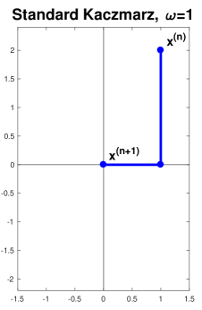
In geometric terms, the Kaczmarz method for this example corresponds to projection onto the -axis and onto a line forming an angle with the -axis.
For standard Kaczmarz, the iteration matrix is
The eigenvalues are
For small , the eigenvalues are real and decreasing as a function of . They become complex at
which is between 1 and 2. After that point, both eigenvalues have magnitude , and the spectral radius increases in a straight line. The dependence of on is illustrated below in the left half of fig. 4. Here , , .
As pointed out in [14], there is a strong connection between the classical Kaczmarz method and Successive Over-Relaxation (SOR). In SOR the relationship between and shows the same type of behavior.
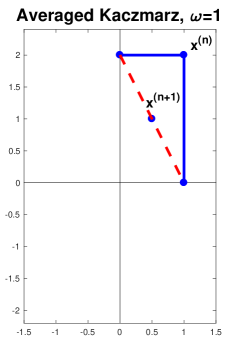
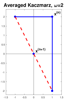
The example with two equations is too small to implement as distributed Kaczmarz, but we consider something similar. We project the same onto each line, and average the result to get . We will refer to this as the averaged Kaczmarz method.
The iteration matrix is
The eigenvalues here are always real and vary linearly with , namely
They both have the value 1 at , and are both decreasing with increasing . The first one reaches at
Thus, the upper limit is somewhere between 2 and 4, depending on . In numerical experiments with the distributed Kaczmarz method for larger matrices, we have observed near 4, but never above 4. We conjecture that can never be larger than 4.
The minimum spectral radius occurs at , independent of , with . The dependence of on is illustrated below in the left half of fig. 4. In this example, the graph for the averaged Kaczmarz method consists of two line segments, with , .
Figure 3 illustrates the optimal for . The optimal for standard Kaczmarz is , with . Convergence occurs in a single step. For the averaged method, the optimal is 2, where again convergence occurs in a single step. The averaged method would still converge for a range of .
Numerical experiments with larger sets of equations indicate that the optimal for classical Kaczmarz is usually larger than 1, but of course cannot exceed 2. The optimal for distributed Kaczmarz is usually larger than 2, sometimes even approaching 4.
Example 2.
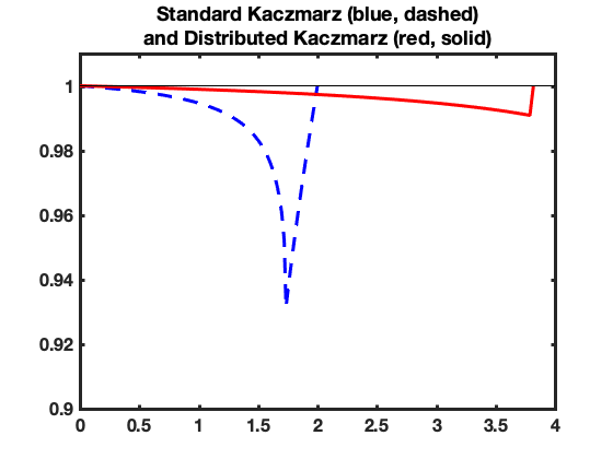
We used a random matrix of size , with entries generated using a standard normal distribution. For the distributed Kaczmarz method, we used the 8-node graph as shown on the right in Figure 5.
For the standard Kaczmarz method, the optimal relaxation parameter was , with spectral radius . For the distributed Kaczmarz method, the results were , with spectral radius . This is illustrated in on the right in figure 4.

3.2. Implementation
The implementation of the distributed Kaczmarz algorithm is based on the Matlab Graph Theory toolbox. This toolbox provides support for standard graphs and directed graphs (digraphs), weighted or unweighted. We are using a weighted digraph. The graph is defined by specifying the edges, which automatically also defines the nodes. Specifying nodes is only necessary if there are additional isolated nodes. Both nodes and edges can have additional properties attached to them. We take advantage of that by storing the equations and right-hand sides, as well as the current approximate solution, in the nodes. The weights are stored in the edges. We are currently only considering tree-structured graphs. One node is the root. Each node other than the root has one incoming edge, coming from the predecessor, and zero or more outgoing edges leading to the successors. A node without a successor is called a leaf.
The basic Kaczmarz step has the form x_new = update_node(node,omega,x). The graph itself is a global data structure, accessible to all subroutines; it would be very inefficient to pass it as an argument every time.
The update_node routine does the following:
-
•
Use the equation(s) in the node to update x
-
•
Execute the update_node routine for each successor node
-
•
Combine the results into a new x, using the weights stored in the outgoing edges
-
•
Return x_new
This routine needs to be called only once per iteration, for the root. It will traverse the entire tree recursively.
3.3. Numerical Experiments
We illustrate the methods with some simple numerical experiments. All experiments were run with three different nonsingular matrices each, of sizes and . All matrices were randomly generated once, and then stored. The right-hand size vectors are also random, and scaled so that the true solution has -norm 1. The test matrices are
-
•
An almost orthogonal matrix, generated from a random orthogonal matrix by truncating to one decimal of accuracy
-
•
A random matrix, based on a standard normal distribution
-
•
A random matrix, based on a uniform distribution in
In each case, we used the optimal , based on minimizing the spectral radius of the iteration matrix numerically. The distributed Kaczmarz method used the graphs shown in Figure 5. Results are shown in Tables 1 and 2. In all cases, we start with , so the initial -error is . refers to the error after 10 iteration steps. For an orthogonal matrix, the standard Kaczmarz method converges in a single step. It is not surprising that it performs extremely well for the almost orthogonal matrices.
| Standard Kaczmarz | Distributed Kaczmarz | |||||
|---|---|---|---|---|---|---|
| orthogonal | 1.00030 | 0.00294 | 0 | 1.33833 | 0.33753 | |
| normal | 1.07213 | 0.20188 | 1.82299 | 0.29611 | ||
| uniform | 1.18634 | 0.37073 | 1.92714 | 0.82562 | ||
| Standard Kaczmarz | Distributed Kaczmarz | |||||
|---|---|---|---|---|---|---|
| orthogonal | 1.01585 | 0.04931 | 1.76733 | 0.73919 | ||
| normal | 1.73543 | 0.93147 | 3.78883 | 0.99087 | ||
| uniform | 1.88188 | 0.92070 | 3.73491 | 0.99890 | ||
Acknowledgements. This research was supported by the National Science Foundation and the National Geospatial-Intelligence Agency under awards DMS-1830254 and CCF-1750920.
References
- [1] Dimitri P. Bertsekas and John N. Tsitsiklis, Parallel and distributed computation: Numerical methods, Athena Scientific, Nashua, NH, 1997, originally published in 1989 by Prentice-Hall; available for free download at http://hdl.handle.net/1721.1/3719.
- [2] Stephen Boyd, Neal Parikh, Eric Chu, Borja Peleato, Jonathan Eckstein, et al., Distributed optimization and statistical learning via the alternating direction method of multipliers, Foundations and Trends® in Machine Learning 3 (2011), no. 1, 1–122.
- [3] Yuejie Chi and Yue M Lu, Kaczmarz method for solving quadratic equations, IEEE Signal Processing Letters 23 (2016), no. 9, 1183–1187.
- [4] P. P. B. Eggermont, G. T. Herman, and A. Lent, Iterative algorithms for large partitioned linear systems, with applications to image reconstruction, Linear Alg. Appl. 40 (1981), 37–67.
- [5] Richard Gordon, Robert Bender, and Gabor Herman, Algebraic reconstruction techniques (ART) for threedimensional electron microscopy and x-ray photography, Journal of Theoretical Biology 29 (1970), no. 3, 471–481.
- [6] C. Hamaker and D. C. Solmon, The angles between the null spaces of X rays, Journal of Mathematical Analysis and Applications 62 (1978), no. 1, 1–23.
- [7] Per Christian Hansen, Discrete inverse problems, Fundamentals of Algorithms, vol. 7, Society for Industrial and Applied Mathematics (SIAM), Philadelphia, PA, 2010, Insight and algorithms. MR 2584074
- [8] G. T. Herman, A. Lent, and H. Hurwitz, A storage-efficient algorithm for finding the regularized solution of a large, inconsistent system of equations, J. Inst. Math. Appl. 25 (1980), no. 4, 361–366. MR 578083
- [9] Gabor T. Herman, Henry Hurwitz, Arnold Lent, and Hsi Ping Lung, On the Bayesian approach to image reconstruction, Inform. and Control 42 (1979), no. 1, 60–71. MR 538379
- [10] Björn Johansson, Maben Rabi, and Mikael Johansson, A randomized incremental subgradient method for distributed optimization in networked systems, SIAM Journal on Optimization 20 (2009), no. 3, 1157–1170.
- [11] Stefan Kaczmarz, Angenäherte Auflöösung von Systemen linearer Gleichungen, Bulletin International de l’Académie Polonaise des Sciences et des Lettres. Classe des Sciences Mathématiques et Naturelles. Série A, Sciences Mathématiques (1937), 355–357.
- [12] Goutham Kamath, Paritosh Ramanan, and Wen-Zhan Song, Distributed randomized Kaczmarz and applications to seismic imaging in sensor network, 2015 International Conference on Distributed Computing in Sensor Systems, 06 2015, pp. 169–178.
- [13] Stanisław Kwapień and Jan Mycielski, On the Kaczmarz algorithm of approximation in infinite-dimensional spaces, Studia Math. 148 (2001), no. 1, 75–86. MR 1881441 (2003a:60102)
- [14] Frank Natterer, The mathematics of computerized tomography, Teubner, Stuttgart, 1986.
- [15] Angelia Nedic and Asuman Ozdaglar, Distributed subgradient methods for multi-agent optimization, IEEE Transactions on Automatic Control 54 (2009), no. 1, 48.
- [16] Deanna Needell, Nathan Srebro, and Rachel Ward, Stochastic gradient descent, weighted sampling, and the randomized Kaczmarz algorithm, Math. Program. 155 (2016), no. 1-2, Ser. A, 549–573. MR 3439812
- [17] Deanna Needell and Joel A. Tropp, Paved with good intentions: analysis of a randomized block Kaczmarz method, Linear Algebra Appl. 441 (2014), 199–221. MR 3134343
- [18] Deanna Needell, Ran Zhao, and Anastasios Zouzias, Randomized block Kaczmarz method with projection for solving least squares, Linear Algebra Appl. 484 (2015), 322–343. MR 3385065
- [19] Ali H Sayed, Adaptation, learning, and optimization over networks, Foundations and Trends® in Machine Learning 7 (2014), no. 4-5, 311–801.
- [20] Kevin Scaman, Francis Bach, Sébastien Bubeck, Laurent Massoulié, and Yin Tat Lee, Optimal algorithms for non-smooth distributed optimization in networks, Advances in Neural Information Processing Systems, 2018, pp. 2740–2749.
- [21] Devavrat Shah, Gossip algorithms, Foundations and Trends® in Networking 3 (2008), no. 1, 1–125.
- [22] Thomas Strohmer and Roman Vershynin, A randomized Kaczmarz algorithm with exponential convergence, Journal of Fourier Analysis and Applications 15 (2009), no. 2, 262–278.
- [23] Kunio Tanabe, Projection method for solving a singular system of linear equations and its application, Numer. Math. 17 (1971), 203–214.
- [24] John Tsitsiklis, Dimitri Bertsekas, and Michael Athans, Distributed asynchronous deterministic and stochastic gradient optimization algorithms, IEEE Transactions on Automatic Control 31 (1986), no. 9, 803–812.
- [25] Douglas B. West, Introduction to graph theory, Prentice Hall, Inc., Upper Saddle River, NJ, 1996. MR 1367739
- [26] Lin Xiao, Stephen Boyd, and Seung-Jean Kim, Distributed average consensus with least-mean-square deviation, Journal of Parallel and Distributed Computing 67 (2007), no. 1, 33–46.
- [27] Kôsaku Yosida, Functional analysis, Second edition. Die Grundlehren der mathematischen Wissenschaften, Band 123, Springer-Verlag New York Inc., New York, 1968. MR 0239384
- [28] Kun Yuan, Qing Ling, and Wotao Yin, On the convergence of decentralized gradient descent, SIAM Journal on Optimization 26 (2016), no. 3, 1835–1854.
- [29] Xin Zhang, Jia Liu, Zhengyuan Zhu, and Elizabeth S. Bentley, Compressed distributed gradient descent: Communication-efficient consensus over networks, 2018, arxiv.org/pdf/1812.04048.