Bifurcation of limit cycles from the global center of a class of
integrable non-Hamilton system under perturbations
of piecewise smooth polynomials
Shiyou Sui, Liqin Zhao∗
School of Mathematical
Sciences, Beijing Normal University,
Laboratory of Mathematics and Complex Systems, Ministry of
Education,
Beijing 100875, The People’s Republic of China
11footnotetext:
* Corresponding author. This work was supported by NSFC(11671040).
E-mail: zhaoliqin@bnu.edu.cn (L. Zhao), suisy@mail.bun.edu.cn(S. Sui).
Abstract In this paper, we perturb the global center of the planar polynomial vector fields () inside cubic piecewise smooth polynomials with switching line . By using average function of first order, we prove that the sharper bound of the number of limit cycles bifurcating from the period annulus is 6.
One of the main problems inside the qualitative theory in the qualitative theory of real planar differential systems is to determine the number of limit cycles which is related to the Hilbert 16th problem [6,11]. A limit cycle is an isolated periodic orbit defined by Poincaré [8]. There are many phenomena in real world related with the existence of limit cycles, some examples are the van der Pol oscillator [20,21], or the Belousov-Zhabotinskii reaction [1,24]. For more about limit cycles, one can see [2,23].
The notion of a center of real planar differential system is an isolated equilibrium point having a neighborhood such that all the orbits of this neighborhood are periodic with the unique exception of the equilibrium point, which is defined by Poincaré [18]. Late on a classic way to obtain limit cycles is perturbing the periodic orbits of a center.
In 1999, Iliev [10] considered the polynomial vector fields
by perturbing it with polynomials of degree . He studied how many limit cycles can bifurcate from the periodic orbits of the linear center. Later on many people studied the perturbations of polynomial vector fields of the form , where , see [13,19,22] and the references they cited.
There are many studies of the limit cycles of continuous and discontinuous piecewise differential systems in with two pieces separated by a straight line. In general these differential systems are linear, see for instance [5,8,9,16]. T. Carvalho, J. Llibre, and D. J. Tonon [4] studied the number of limit cycles which can bifurcate from the nonlinear center , when it is perturbed inside a class of discontinuous piecewise polynomial differential systems of degree with pieces. S. Li and Ch. Liu [12] studied the piecewise smooth differential system
where are polynomials of degree .
In this paper, we will study the number of limit cycles which can bifurcate from the center of
when it is perturbed inside discontinuous piecewise cubic polynomials, where . Let , then system (1.1) is transformed into
here we omit the subscript 1. Hence, we consider the following perturbations of system (1.2)
where , are arbitrary constants, the characteristic function of a set is defined by
and .
The system has a periodic annulus surround the origin. Then, using average function of first order (see Section 2), we find the maximum number of limit cycles of system (1.3). The main results of this paper is the following.
Theorem 1.1. Suppose that the average function of first order associated to the discontinuous piecewise polynomial differential system (1.3) is non-zero. Then for sufficiently small the sharper bound of the number of limit cycles of system (1.3) is 6.
Corollary 1.2. Under the assumption of theorem 1.1, if , for sufficiently small the sharper bound of the number of limit cycles of system (1.3) is 3.
Remark 1.3. Using the results of [22], we know that system under the perturbation of smoth polynomials with degree has at most .
This paper is organized as follows. In Section 2, we introduce averaging theory for computing periodic solution and extend complete Chebyshev system for studying the number of zeros of average function. The main results is proved in Section 3.
. Preliminary results
In this section we summarize the main tools that we will use to study the bifurcation of limit cycles for system (1.3). First, we introduce the averaging theory for discontinuous piecewise differential systems. The following results stated on the averaging theory are valid for discontinuous piecewise polynomial vector field defined in and are proved in [15], but we shall state them for our discontinuous piecewise polynomial vector field (1.3) in polar coordinates.
Consider a non-autonomous discontinuous piecewise vector field
where , and
where , for are continuous functions, -periodic in the variable , and is an open interval of . Here the are the open intervals for and . We define
The average function is defined by
We recall that if is the solution of the vector field such that , then we have
So for suffieiently small the simple zeros of the averaged function provides limit cycles of the vector field .
In the next result we present a version of the averaging theory for discontinuous piecewise vector fields, that is proved in [15], adapted to differential equation (2.1). We note that in [15] the averaging theory uses that the Brouwer degree of a function in a neighborhood of a zero of the function is non-zero, while here we substitute this condition saying that the zero is simple (i.e. ), because this last condition implies that the mentioned Brouwer degree non-zero. See for more details [3,17].
Lemma 2.1. Assume that the following conditions hold for the discontinuous piecewise vector field .
(i) For the functions and are locally Lipschitz with respect to , and -periodic with respect to .
(ii) Let be a simple zero of the average function .
Then for sufficiently small, there exists a -periodic solution of the vector field such that as .
In order to study the number of zeros of the averaging function we will use the following results.
Definition 2.2.([14]) Let be a set and let , we say that are linearly independent functions if and only if we have that
Lemma 2.3.([14]) If are linearly independent then there exit and such that for every
Definition 2.4.([7]) Let be analytic functions on an open interval of .
(a) is a Chebyshev system (in short, T-system) on if any nontrivial linear combination
has at most isolated zeros on .
(b) is an complete Chebyshev system (in short, CT-system) on if is a T-system for all .
(c) is an extend complete Chebyshev system (in short, ECT-system) on if, for all , any nontrivial linear combination
has at most isolated zeros on counted with multiplicities.
It is clear that if is an EXT-system on , then is a CT-system on . However, the reverse implication is not true.
Lemma 2.5.([7]) is an ECT-system on if and only if for each the continuous Wronskian of at is not zero, that is
By Definition 2.2 and Lemma 2.5, it is easy to get the following.
Proposition 2.6. If is an ECT-system on , then they are linearly independent.
. Proof of main results
Using the change to polar coordinates , we transform the differential system (1.3) into
Taking as the new independent variable the previous differential system becomes the differential equation
where
Therefore, the average function of first order is
where . Note that are also arbitrary, since are arbitrary.
In order to simplify the notation, we define the following functions:
Then, it is easy to check that
Notice that in the interval , the zeros of the function coincide with the zeros of the function . Therefore, in order to simplify further computation, we will study the function instead of .
Using above notation, we can obtain that
(3.2)
where . Note that are independent, since are arbitrary.
By direct computation we have the following:
Substituting (3.3) into (3.2), we have that
(3.4)
where
It follows from direct computation that
By the arbitrariness of , we have that are independent. Hence, the generating functions of are the following:
Next, we will prove that is an ECT-system. We introduce the notation
. Direct computation, we have
It is obvious that on .
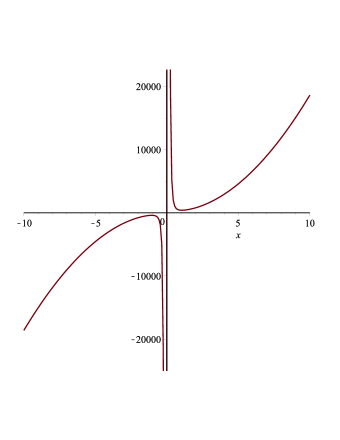
Figure 1: The curve of .
For , using mathematical soft such as Maple, we get that
where
Then,
From the curve (Figure 1) of , we know that on .
So, we get that . Hence, on .
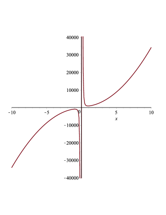
When , we have
where
By the curve (see Figure 2) of , we have that on .
Figure 2: The curve of .
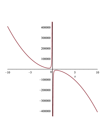
When , we have
where
Figure 3: The curve of .
Then,
and
where
From the curve (see Figure 3) of , we know on .
Hence, on . Therefore, we have that . That is equivalent to on . Thus, , which implies on .
By above analysis we have proved that is an ECT-system on . So, by Lemma 2.5, has at most 6 zeros on . Using proposition 2.6 and Lemma 2.3, we have that can have 6 zeros on . Hence, by Lemma 2.1, theorem 1.1 is proved.
If , then , which imply (i is odd). Then, the generating functions of become
It is easy to check that is an ECT-system on . Then, we ends the proof of Corollary 1.2.
References
[1] B. P. Belousov, Periodically acting reaction and its mechanism, in: Collection of Abstracts on Radiation Medicine, Moscow, 1958, pp. 145-147.
[2] M. di Bernardo, C. J. Budd, A. R. Champneys, P. Kowalczyk, Piecewise-Smooth Dynamical Systems: Theory and Applications, Appl. Math. Sci. Ser., vol. 163, Springer-Verlag, London, 2008.
[3] F. Browder, Fixed point theory and nonlinear problems, Bull. Amer. Math. Soc. 9 (1983) 1-39.
[4] T. Carvalho, J. Llibre, D. Tonon, Limit cycles of discontinuous piecewise polynomial vector fields, J. Math. Anal. Appl. 449 (2017) 572-579.
[5] E. Freire, E. Ponce, F. Torres, Canonical discontinuous planar piecewise linear system, SIAM J. Appl. Dyn. Syst. 11 (2012) 181-211.
[6] J. Giné, On some open problems in planar differential systems and Hilbert’s 16th problem, Chaso, Solitons and Fractals 31 (2007) 1118-1134.
[7] M. Grau, F. Mañosas, J. Villadelprat, A Chebyshev criterion for Abelian integrals, Trans. Amer. Math. Soc. 363 (2011) 109-129.
[8] M. Han, W. Zhang, On Hopf bifurcation in non-smooth planar systems, J. Differential Equations 248 (2010) 2399-2416.
[9] S. Huan, X. Yang, On the number of limit cycles in genreal planar piecewise linear systems, Discrete Contin. Dyn. Syst. Ser. A 32 (2012) 2147-2164.
[10] I. D. Iliev, The number of limit cycles due to polynomial perturbations of the harmonic oscillator, Math. Proc. Cambridge Philos. Soc. 127 (1999) 317-322.
[11] Ch. Li, Abelian integrals and limit cycles, Qual. Theory Dyn. Syst. 11 (2012) 111-128.
[12] S. Li, Ch. Liu, A linear estimate of the number of limit cycles for some planar piecewise smooth quadratic differential system, J. Math. Anal. Appl. 428 (2015) 1354-1367.
[13] S. Li, Y. Zhao, J. Li, On the number of limit cycles of a perurbed cubic polynomial differential center, J. Math. Anal. Appl. 404 (2013) 212-220.
[14] J. Llibre, A.C. Mereu, Limit cycles for discontinuous quadratic differential systems with two zones, J. Math. Anal. Appl. 413 (2014) 763-775.
[15] J. Llibre, A.C. Mereu, D.D. Novaes, Averaging theory for discontinuous piecewise differential systems, J. Differential Equations 258 2015 4007-4032.
[16] J. Llibre, X. Zhang, Limit cycles for discontinuous planar piecewise linear differential system separated by one straight line and having a center, J. Math. Anal. Appl. 467 (2018) 537-549.
[17] N.G. Lloyd, Degree Theory, Cambridge University Press,1978.
[18] H. Poincaré, Mémoire sur les courbes définies par une équation differentielle I, II, J. Math. Pures Appl. 7 (1881) 375-422; 8 (1882) 251-296;
H. Poincaré, Sur les courbes définies par les équation differentielles III, IV, 1 (1885) 167-244; 2 (1886) 155-217.
[19] S. Sui, L. Zhao, Bifurcation of limit cycles from the center of a family of cubic polynomial vector fields, Internat. J. Bifur. Chaos Appl. Sci. Engrg. 28 (2018) 1850063 (11 pages).
[20] B. Van der Pol, A theory of the amplitude of free and forced triode vibrations, Radio Rev. 1 (1920) 701-710 (later Wireless World).
[21] B. Van der Pol, On relaxation-oscillations, Philos. Mag. 2 (7) (1926) 978-992.
[22] G. Xiang, M. Han, Global bifurcation of limit cycles in a family of polynomial, J. Math. Anal. Appl. 295 (2004) 633-644.
[23] Y. Ye, Theory of limit cycles, Transl. Math. Monogr., vol. 66, Amer. Math. Soc., Providence, RI, 1986.
[24] A. M. Zhabotinsky, Periodical oxidation of malonic acid in solution (a study of the Belousov reaction kinetics), Biofizika 9 (1964) 306-311.