Thermalization of hot electrons via interfacial electron-magnon interaction

Abstract

Recent work on layered structures of superconductors (S) or normal metals (N) in contact with ferromagnetic insulators (FI) has shown how the properties of the previous can be strongly affected by the magnetic proximity effect due to the static FI magnetization. Here we show that such structures can also exhibit a new electron thermalization mechanism due to the coupling of electrons with the dynamic magnetization, i.e., magnons in FI. We here study the heat flow between the two systems and find that in thin films the heat conductance due to the interfacial electron-magnon collisions can dominate over the well-known electron-phonon coupling below a certain characteristic temperature that can be straightforwardly reached with present-day experiments. We also study the role of the magnon band gap and the induced spin-splitting field induced in S on the resulting heat conductance and show that heat balance experiments can reveal information about such quantities in a way quite different from typical magnon spectroscopy experiments.

I Introduction

The progress in low temperature solid state device technology, such as thermometry and electromagnetic radiation detection Irwin and Hilton (2005); Grossman et al. (1991); Bluzer and Forrester (1994); Sergeev et al. (2002); Giazotto et al. (2008); Govenius et al. (2016); Giazotto et al. (2006); Heikkilä et al. (2018); Chakraborty and Heikkilä (2018), electron refrigeration Kawabata et al. (2013); Rouco et al. (2018) and new solutions for quantum information processing Lian et al. (2018), call for an improved understanding of the thermalization mechanisms. This is particularly relevant at their usual sub-Kelvin operating temperatures and in hybrid structures. We schematically represent an example hybrid structure in Fig. 1, based on a thin-film normal metal (N) or a thin-film superconductor (S) in contact with a thin-film ferromagnetic insulator (FI). It can be a part of some low-temperature thermometric device, such as a thermoelectric radiation detector (TED) Heikkilä et al. (2018); Chakraborty and Heikkilä (2018). When such devices are operated, they are often brought out of equilibrium via a process involving absorption of an electromagnetic field with power $P_{\gamma}$. This power may be the one under study as in radiation detectors, or one inadvertently brought in when operating the device. As schematized in Fig. 1, this power initially heats up the electrons of the N or S, and then the hot electrons dissipate the heat via coupling to larger heat baths, typically via coupling to the phonons (ph) Wellstood et al. (1994); Giazotto et al. (2006); Timofeev et al. (2009); Maisi et al. (2013); Bergeret et al. (2018). In systems with ferromagnetic elements, such as the one shown in Fig. 1, the electrons can also couple to the magnons, which can then conduct the energy away from the heated region. This mechanism we study in this paper.

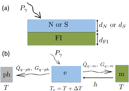
Figure 1: (a) Schematic of a hybrid bilayer of a normal metal (N) or a superconductor (S) of thickness $d_{N}$ or $d_{S}$ in a good contact with a ferromagnetic insulator (FI) of thickness $d_{\mathrm{FI}}$. (b) $P_{\gamma}$ denotes the incident radiation power, which increases the electronic temperature by an amount $\Delta T$ from some initial temperature $T$ dictated by the temperature of the baths. For a low and constant power $P_{\gamma}$, the magnitude of $\Delta T=P_{\gamma}/G_{\rm th}^{\rm tot}$ is dictated by the total heat conductance, $G_{\rm th}^{\rm tot}$, to the heat bath. This heat conductance is typically due to the coupling of the electrons (e) to the phonons (ph), but at a low enough temperature also magnons (m) in the FI film start to be relevant, and eventually may become the dominant heat conduction mechanism. Here $h$ denotes the spin-splitting field possibly induced to N or S via the magnetic proximity effect. $\dot{Q}_{\rm q-ph}$ and $\dot{Q}_{\rm q-m}$ stand for the rates of heat flow due to electron-phonon interaction and electron-magnon collisions, respectively and $G_{\rm q-ph}$ and $G_{\rm q-m}$ are the corresponding heat conductances.

The interfacial electron-magnon interaction strength can be quite large, and hence important for the thin film materials, as the recent work on superconductivity induced in a metal due to interfacial electron-magnon interaction Rohling et al. (2018), and spin transport across normal metal and ferromagnetic insulator Bender et al. (2012); Takahashi et al. (2010) suggest. There have been various research works, such as spin pumping, spin and charge tunneling current in magnetic multilayered structures Tserkovnyak et al. (2002); Mahfouzi and Nikolić (2014); Cheng et al. (2017); Tveten et al. (2015); Schreier et al. (2013), which one can also independently analyze via interfacial electron-magnon interaction. In this work we demonstrate that the electron-magnon heat flow can be as important as electron-phonon heat conduction below a certain characteristic temperature, for a certain regime of electron-magnon interaction strength, magnon band gap and spin-splitting field. At high temperatures electron-phonon heat flow dominates over electron-magnon heat flow. The dominance of the interfacial electron-magnon heat flow over electron-phonon heat transport in the bulk below a characteristic temperature is due to the difference of the magnon and phonon dispersions, and hence the dissimilarity in the magnon density of states at the N-FI or S-FI interface and the phonon density of states in the bulk.

Our present work is especially important in the context of proposals for a new kind of a low temperature thermoelectric radiation detector (TED) Heikkilä et al. (2018); Chakraborty and Heikkilä (2018), which can rival the contemporary device technologies, such as transition edge sensor (TES) and kinetic inductance detector (KID) Irwin and Hilton (2005); Grossman et al. (1991); Bluzer and Forrester (1994); Sergeev et al. (2002); Giazotto et al. (2008); Govenius et al. (2016). The TED is based on a combination of a thin film spin-split superconductor with a spin-polarized tunnel junction, and it utilizes the recently discovered giant thermoelectric effect in superconductor-ferromagnet hybrid structures Ozaeta et al. (2014); Machon et al. (2013, 2014); Kolenda et al. (2016, 2017); Rezaei et al. (2018); Bergeret et al. (2018). Spin-split superconductors can also be used to generate different types of devices combining thermoelectricity and the macroscopic phase coherence of the superconducting state Giazotto et al. (2014, 2015). One way to realize the spin-split superconductor is to couple the S with FI. Such devices are the most sensitive at the lowest temperatures reached. This is why understanding the thermalization mechanisms directly improves the design of such devices.

In what follows we first present the theory of electron-magnon heat transport in N-FI and S-FI contacts. Then we discuss our results on electron-magnon heat conductance and compare it with electron-phonon heat conductance of N or S to establish the regime where the previous dominates.

II Theoretical model

To study the heat conduction due to interfacial electron-magnon collisions in N-FI or S-FI hybrid structures, we consider the effective model Hamiltonian

$$\hat{H} = \hat{H}_{e}+\hat{H}_{em}+\hat{H}_{m},$$ (1)

$$\hat{H}_{e} = \sum_{\vec{k}\sigma}(\epsilon_{\vec{k}\sigma}-\mu)c^{\dagger}_{\vec{k}\sigma}c_{\vec{k}\sigma}~{}~{}~{}~{}~{}~{}~{}\mathrm{for~{}N},$$ (2)

$$= \sum_{\vec{k}\sigma}E_{\vec{k}\sigma}\gamma^{\dagger}_{\vec{k}\sigma}\gamma_{\vec{k}\sigma}~{}~{}~{}~{}~{}~{}~{}~{}~{}~{}~{}~{}~{}\mathrm{for~{}S},$$

$$\hat{H}_{m} = \sum_{\vec{q}}\omega_{\vec{q}}a^{\dagger}_{\vec{q}}a_{\vec{q}},$$ (3)

$$\hat{H}_{em} = -g_{em}\sum_{\vec{k},~{}\vec{q}}c^{\dagger}_{\vec{k}\uparrow}c_{\vec{k}+\vec{q}\downarrow}a^{\dagger}_{\vec{q}}+\mathrm{h.c}.$$ (4)

Here $\hat{H}_{e}$, $\hat{H}_{m}$ and $\hat{H}_{em}$ stand for the Hamiltonian of the quasi two-dimensional (thin film) N or S, for the quasi two-dimensional FI Van Kranendonk and Van Vleck (1958) and the electron-magnon interaction due to the N-FI or S-FI contact Rohling et al. (2018). We assume low enough temperatures so that the thickness $d_{N/S}$ satisfies $d_{N/S}\ll 2\pi\hbar v_{F}/(k_{B}T)$, where $v_{F}$ is the Fermi velocity of the electronic system and $T$ is the temperature. In this case the thin films can be considered effectively two-dimensional and the sums over $\vec{k},\vec{q}$ in Eqs. (2)-(4) are also two-dimensional.

In Eq. (2) we denote the electron energy $\epsilon_{\vec{k}\sigma}=\epsilon_{\vec{k}}-h\sigma$ for spin $\sigma$, where $\sigma=\pm 1$ for $\sigma=\uparrow/\downarrow$, and the spin dependent Bogoliubon energy $E_{\vec{k}\sigma}=E_{\vec{k}}-h\sigma$. Hence $\epsilon_{\vec{k}}=\mu+\hbar v_{F}(k-k_{F})$ and $E_{\vec{k}}=\sqrt{(\epsilon_{\vec{k}}-\mu)^{2}+\Delta^{2}}$, where $\mu$ and $k_{F}$ are the chemical potential and the magnitude of the Fermi wave vector in the N or S. $\Delta$ is the superconducting gap of S and $h$ stands for the spin-splitting field exerted on N or S due to FI. In Eq. (3) $\omega_{\vec{q}}=\omega_{0}+Bq^{2}$ represents the magnon energy dispersion relation in FI, with $\omega_{0}\geq 0$ and $B=J_{\mathrm{ex}}zs\zeta^{2}/2>0$ Van Kranendonk and Van Vleck (1958), where $J_{\mathrm{ex}}$, $s$, $z$ and $\zeta$ are the isotropic exchange coupling energy, effective lattice spin, coordination number and the lattice constant of FI, respectively. The effective electron-magnon coupling energy is defined as $g_{em}\sqrt{A}=-J\zeta\sqrt{2s}$, where $A$ is the area of the contact surface, $J$ is the exchange energy between the electrons of the N or S with FI and $\zeta^{2}=A/N_{0}$ where $N_{0}$ is the number of lattice points of FI at the surface of the N-FI or S-FI contact. In Eqs. (2)-(4) $c$, $\gamma$ and $a$ are the annihilation operators for the electrons of the N or S, Bogoliubon operator of S and magnon operator for FI, respectively. For S we have $c_{\vec{k}\sigma}=v_{\vec{k}\sigma}\gamma^{\dagger}_{-\vec{k}-\sigma}+u^{*}_{\vec{k}\sigma}\gamma_{\vec{k}\sigma}$, $\left|u_{\vec{k}\sigma}\right|^{2}+\left|v_{\vec{k}\sigma}\right|^{2}=1$, $u_{\vec{k}\uparrow}=u_{\vec{k}}$, $u_{\vec{k}\downarrow}=u_{\vec{k}}$, $v_{\vec{k}\uparrow}=v_{\vec{k}}$ and $v_{\vec{k}\downarrow}=-v_{-\vec{k}}$, $\Delta^{*}v_{\vec{k}}/u_{\vec{k}}=E_{\vec{k}}-(\epsilon_{\vec{k}}-\mu)$, $2\left|v_{\vec{k}}\right|^{2}=\left[1-\left({\epsilon_{\vec{k}}-\mu}\right)/{E_{\vec{k}}}\right]$.

Using the Hamiltonians of Eqs. (1)-(4), we calculate the heat flow from the magnons of the FI to the electrons of the N or S, according to the Kubo linear response theory, as $\left<\dot{\hat{H}}_{m}(t)\right>=\left<\dot{\hat{H}}_{m}(t)\right>_{0}-\frac{i}{\hbar}\int_{-\infty}^{t}dt^{\prime}\left<\left[\dot{\hat{H}}_{m}(t),\hat{H}_{em}(t^{\prime})\right]\right>_{0}$ Kubo (1957). Here $\left<\cdot\cdot\cdot\right>_{0}$ stands for thermal averaging over the non-interacting system. As a result we obtain the rate of heat flow from the magnons to the electrons as

$$\lim_{t\to\infty}\left<\dot{\hat{H}}_{m}(t)\right> =\Lambda\left(Q_{\rm q-m}^{(+)}-Q_{\rm q-m}^{(-)}\right),$$ (5)

$$\Lambda =\frac{(k_{F}^{2}J\zeta\sqrt{2s})^{2}}{(16\pi^{2}\hbar\mu^{2})}$$ (6)

and

$$Q_{\rm q-m}^{(\pm)} = 2\int_{-\infty}^{\infty}dE\int_{\omega_{0}}^{4\omega_{F}+\omega_{0}}d\omega\left[n(\omega,T_{e})-n(\omega,T)\right]$$ (7)

$$\times K^{(\pm)}(E,\omega)\left[f(E\mp\omega,T_{e})-f(E,T_{e})\right],$$

where $n(x,T)=\left[\exp[x/(k_{B}T)]-1\right]^{-1}$ and $f(x,T)=\left[\exp[x/(k_{B}T)]+1\right]^{-1}$ are the Bose-Einstein and Fermi-Dirac distributions, respectively. $\omega_{F}=Bk_{F}^{2}$ is the magnon equivalent of the Bloch-Grüneisen energy, originating from the requirement for simultaneous energy and momentum conservation. $T$ and $T_{e}$ are the temperatures of the magnons and electrons. The matrix element of the coupling results into the kernel terms $K^{(\pm)}(E,\omega)$, which are given below for normal and superconducting metals coupled to the ferromagnetic insulator [Eqs. (10) and (14), respectively]. Finally let us obtain the electron-magnon heat conductance, $G_{\rm q-m}$, within linear response $\Delta T=T_{e}-T\ll T$ as

$$G_{\rm q-m}=\lim_{t\to\infty}\frac{\left<\dot{\hat{H}}_{m}(t)\right>}{\Delta T}=\Lambda A\left(G_{\rm q-m}^{(+)}-G_{\rm q-m}^{(-)}\right),$$ (8)

where

$$G^{(\pm)}_{\rm q-m} = \frac{1}{2k_{B}T^{2}}\int_{-\infty}^{\infty}dE\int_{\omega_{0}}^{4\omega_{F}+\omega_{0}}d\omega~{}\omega\sinh^{-2}\left(\frac{\omega}{2k_{B}T}\right)$$ (9)

$$\times K^{(\pm)}(E,\omega)\left[f(E\mp\omega,T)-f(E,T)\right].$$

The steps leading to Eqs. (5)-(9) correspond to the Born approximation similar to the one used for studying electron-phonon heat transport in earlier works Wellstood et al. (1994); Timofeev et al. (2009); Maisi et al. (2013).

In what follows we assume $k_{B}T$, $h$, $\omega_{\vec{q}}$ and $\omega_{F}\ll\mu$, where $\omega_{\vec{q}}$ are the relevant magnons at low temperatures. As a result, we obtain the kernel term for N-FI as (see the discussion in Appendix A) $K^{(\pm)}(E,\omega)=K(\omega)$ with

$$K(\omega)=\sqrt{\frac{\omega}{\omega_{F}}}\sqrt{\frac{\omega}{\omega-\omega_{0}}}\left[4-\left(\frac{\omega-\omega_{0}}{\omega_{F}}\right)\right]^{-1/2}.~{}~{}~{}~{}$$ (10)

Since the kernel is independent of $E$, we can perform the integral over $E$ in Eq. (8) and obtain

$$G_{\rm q-m} = \frac{\Lambda A}{k_{B}T^{2}}\int_{\omega_{0}}^{4\omega_{F}+\omega_{0}}d\omega K(\omega)\omega^{2}\sinh^{-2}\left(\frac{\omega}{2k_{B}T}\right).~{}~{}~{}~{}$$ (11)

The remaining integral cannot be evaluated analytically, but we can study its different limiting cases. We get

$$G_{\rm q-m} = \Lambda Ak_{B}\frac{\sqrt{\pi}e^{-\omega_{0}/(k_{B}T)}\left[8\omega_{0}^{3}+12k_{B}T\omega_{0}^{2}+18(k_{B}T)^{2}\omega_{0}+15(k_{B}T)^{3}\right]}{4(k_{B}T)^{3/2}\omega_{F}^{1/2}},\quad\text{for }k_{B}T\ll\omega_{0}\ll\omega_{F}$$ (12a)

$$= \Lambda Ak_{B}L_{0}\frac{(k_{B}T)^{3/2}}{\omega_{F}^{1/2}},\quad\text{for }\omega_{0}\ll k_{B}T\ll\omega_{F}$$ (12b)

$$= \Lambda Ak_{B}\frac{\pi[\omega_{0}+2\omega_{F})(12(k_{B}T)^{2}-10\omega_{F}^{2}-4\omega_{0}\omega_{F}-\omega_{0}^{2}]}{3(k_{B}T)^{2}},\quad\text{for }\omega_{0},\omega_{F}\ll k_{B}T.$$ (12c)

Here $L_{0}=\int_{0}^{\infty}dxx^{5/2}[\cosh(x)-1]^{-1}\approx 8.91647.$ Note that as a function of temperature, $G_{\rm q-m}$ is monotonically increasing, but it saturates when $k_{B}T\gg\omega_{F}$. On the other hand, with respect to both the magnon band-gap $\omega_{0}$ and the Bloch-Grüneisen type parameter $\omega_{F}$ the behavior is non-monotonous when $\omega_{0}\ll\omega_{F}$, with a maximal value obtained when $\omega_{F/0}$ is of the order of $k_{B}T$.

To compare the electron-magnon heat conductance $G_{\rm q-m}$ of the thin film N-FI with the electron-phonon heat conductance, we here consider the bulk electron-phonon heat conductance of N as Wellstood et al. (1994),

$$G_{\rm q-ph}=5\Sigma\Omega T^{4},$$ (13)

where $\Sigma$ is the material dependent electron-phonon coupling constant and $\Omega$ is the volume of the quasi two-dimensional N. Comparing the analytical estimate of $G_{\rm q-m}$ in Eqs. (12a)-(12c) with $G_{\rm q-ph}$ in Eq. (13), we conclude that for small magnon band gaps at relatively low temperatures where $\omega_{0}\ll k_{B}T\ll\omega_{F}$, the electron-magnon heat conductance can dominate over the electron-phonon mechanism, whereas at high temperatures the electron-phonon heat conductance is the dominant thermalization mechanism. The relative importance of these two processes changes at a crossover temperature, where both heat conductances are equal to each other. Note that $G_{\rm q-ph}$ in Eq. (13) is obtained after assuming a continuous spectrum of three-dimensional wave vectors, whereas for the electron-magnon heat conductance we include only a two-dimensional integral. The latter is primarily due to the fact that in the N-FI bilayer the electron-magnon coupling is a surface effect, and secondarily due to our assumption of thin films. In thin films then Eq. (13) overestimates the actual electron-phonon heat conductance and underestimates the crossover temperature. In addition, the interface could in principle have some dynamical modes (say, some charges hopping from one place to another), but these would have to connect to the continuum to realize a full heat conductance for bulk materials. They hence do not form a new channel, but can modify the coupling constants. We here disregard such effects due to their non-generic nature.

Motivated by the detector application, we also study the electron-magnon heat transport for the quasi two-dimensional S-FI hybrid structure. The kernel term in this case is (see the discussion in Appendix A)

$$K^{(\pm)}(E,\omega) = \sqrt{\frac{\omega}{\omega_{F}}}\sqrt{\frac{\omega}{\omega-\omega_{0}}}N_{S}(E\mp h)N_{S}(E\pm h\mp\omega)\Theta(E)$$ (14)

$$\times\left[1+\Theta(E\pm h\mp\omega)\frac{\Delta^{2}}{(E\mp h)(E\pm h\mp\omega)}\right]\left[4-\left(\frac{\omega-\omega_{0}}{\omega_{F}}\right)\right]^{-1/2},$$

where $N_{S}(E)=\left|\mathrm{Re}\left[{(E+i\Gamma)}/{\sqrt{(E+i\Gamma)^{2}-\Delta^{2}}}\right]\right|$ is the reduced superconducting density of states, $\Gamma\ll\Delta$ is the Dynes parameter Dynes et al. (1984) and $\Theta(x)$ is the Heaviside function. Note that Eq. (14) couples the two different spin components of the superconducting density of states. This is due to the spin-flip mechanism via electron-magnon interaction, as Eq. (4) represents. Now, using Eqs. (5)-(9) and (14) and considering $\omega_{0}=h=0$, $k_{B}T<\Delta\ll 2\omega_{F}$ we analytically estimate the electron-magnon heat conductance of S-FI film as (see the derivation in Appendix B)

$$G_{\rm q-m} = \frac{k_{B}^{5/2}T^{3/2}\Lambda A}{\sqrt{\omega_{F}}}\left(\tilde{\Delta}e^{-\tilde{\Delta}}\sum_{n=0}^{\infty}\frac{D_{n}}{\tilde{\Delta}^{n}}+\tilde{\Delta}^{5/2}e^{-2\tilde{\Delta}}\sum_{n=0}^{\infty}\frac{E_{n}}{\tilde{\Delta}^{n}}\right),$$ (15)

where $\tilde{\Delta}=\Delta/k_{B}T$. The lowest-order coefficients are $D_{0}=4.82$, $D_{1}=2.88$, $E_{0}=\sqrt{2}\pi$ and $E_{1}=\pi/\sqrt{2}$. The two sums in Eq. (15) are for quasiparticle-magnon scattering and magnon driven quasiparticle recombination, respectively. Contrary to the electron-phonon heat conductance discussed below, the scattering term dominates at all temperatures, so the recombination term can also be disregarded to the first approximation. The analytical estimate reveals the dominant exponential decay of $G_{\rm q-m}$ at low temperatures $k_{B}T\ll\Delta$. As $k_{B}T$ approaches $\Delta$, $G_{\rm q-m}$ follows a linear combination of different power laws as a function of temperature.

We compare the electron-magnon heat conductance of the thin film S-FI with the electron-phonon heat conductance of the superconductor, obtained from Heikkilä et al. (2018); Bergeret et al. (2018); Heikkilä et al. (2019)

$$G_{\rm q-ph}=\frac{\Sigma\Omega}{96\zeta(5)k_{B}^{6}T^{2}}\int_{-\infty}^{\infty}dE~{}E\int_{-\infty}^{\infty}d\omega~{}\omega^{2}|\omega|$$

$$~{}~{}~{}~{}~{}~{}~{}~{}~{}~{}~{}\times L_{E,E+\omega}F_{E,\omega},$$ (16a)

$$L_{E,E^{\prime}}=\frac{1}{2}\sum_{\sigma=\uparrow,\downarrow}N_{\sigma}(E)N_{\sigma}(E^{\prime})$$

$$~{}~{}~{}~{}~{}~{}~{}~{}\times\left[1-\Delta^{2}/[(E+\sigma h)(E^{\prime}+\sigma h)]\right],$$ (16b)

$$F_{E,\omega}=-\frac{1}{2}\left[\sinh\left(\frac{\omega}{2k_{B}T}\right)\cosh\left(\frac{E}{2k_{B}T}\right)\right.$$

$$~{}~{}~{}~{}~{}~{}~{}~{}~{}~{}\times\left.\cosh\left(\frac{E+\omega}{2k_{B}T}\right)\right]^{-1},$$ (16c)

where $\Sigma$ is the material dependent electron-phonon coupling constant, $\Omega$ is the volume of the film, $N_{\sigma}(E)=N_{S}(E+\sigma h)$ where $\sigma=\pm 1$ for $\sigma=\uparrow/\downarrow$, and $\zeta(5)$ is the Riemann zeta function. The analytical estimate of the bulk value of $G_{\rm q-ph}$ is Heikkilä et al. (2018); Bergeret et al. (2018)

$$G_{\rm q-ph}\approx\frac{\Sigma\Omega}{96\zeta(5)}T^{4}\left[\cosh(\tilde{h})e^{-\tilde{\Delta}}f_{1}(\tilde{\Delta})\right.$$

$$~{}~{}~{}~{}~{}~{}~{}~{}~{}~{}~{}\left.+\pi\tilde{\Delta}^{5}e^{-2\tilde{\Delta}}f_{2}(\tilde{\Delta})\right],$$ (17)

where $\tilde{h}=h/k_{B}T$ and $\tilde{\Delta}=\Delta/k_{B}T$. In Eq. (17) the terms $f_{1}$ and $f_{2}$ represent the scattering and recombination processes. The latter dominates over the previous for $k_{B}T\gtrsim 0.1\Delta$ and vice versa, so both terms need to be taken into account. The functions $f_{1}(x)=\sum_{n=0}^{3}C_{n}/x^{n}$ and $f_{2}(x)=\sum_{n=0}^{2}B_{n}/x^{n}$, where $C_{0}=440$, $C_{1}=-500$, $C_{2}=1400$, $C_{3}=-4700$, $B_{0}=64$, $B_{1}=144$, $B_{2}=258$. Comparing the two analytical estimates, for $G_{\rm q-m}$ in Eq. (15) and for $G_{\rm q-ph}$ in Eq. (17), we note that the electron-magnon thermalization process can dominate the electron-phonon process at low temperatures, whereas electron-phonon is the dominating mechanism at high temperatures. As a result there can be a crossover temperature, where both heat conductances are equal to each other. Here also it is important to note, as in the case without superconductivity, that Eqs. (16a)-(16c) and (17) are obtained assuming the continuous spectrum of three-dimensional wave vectors of the superconducting electrons, whereas for the electron-magnon heat conductance we include only a two-dimensional integral. As a result this overestimates $G_{\rm q-ph}$ and underestimates the resulting crossover temperature.

III Results and discussions

In what follows we numerically analyze the electron-magnon heat conductance of the thin film normal metal-ferromagnetic insulator, N-FI, and the thin film superconductor-ferromagnetic insulator, S-FI, hybrid structures. We also compare the electron-magnon heat conductance with the bulk electron-phonon heat conductance in the absence and in the presence of superconductivity.

III.1 Normal metal-ferromagnetic insulator

Here we first discuss the electron-magnon heat conduction in a thin film N-FI hybrid structure. In Fig. 2, we plot the electron-magnon heat conductance $G_{\rm q-m}$ vs temperature $T$, for various magnon band gaps $\omega_{0}$ and compare with the analytical estimate of $G_{\rm q-m}$ for $\omega_{0}=0$. In line with Eqs. (12a)-(12c), we find that $G_{\rm q-m}$ decreases exponentially with a decreasing $T$ for $k_{B}T\ll\omega_{0}$, and reaches a constant value, $4\pi k_{B}\Lambda A(\omega_{0}+2\omega_{F})$, for $k_{B}T\gg\omega_{F}$. Figure 2 also contains the bulk electron-phonon heat conductance $G_{\rm q-ph}$ of the thin film N vs $T$ for various film thicknesses $d_{N}$ of the normal metal. To find out the relative importance between electron-magnon and the usual electron-phonon thermalization mechanisms, we now compare $G_{\rm q-m}$ with $G_{\rm q-ph}$. For the comparison, we define a crossover temperature $T^{*}$, where the $G_{\rm q-ph}$ vs $T$ curve crosses the $G_{\rm q-m}$ vs $T$ curve. At the characteristic temperature we thus have

$$G_{\rm q-m}(T=T^{*})=G_{\rm q-ph}(T=T^{*}).$$ (18)

Since the electron-magnon heat conduction is an interface process, and the electron-phonon conduction is a bulk process, the crossover temperature depends on the normal metal thickness $d_{N}$. As expected, we can see from Fig. 2 that the electron-magnon process dominates below $T^{*}$ and vice versa for the electron-phonon process. Using Eqs. (12b) and (13), we get

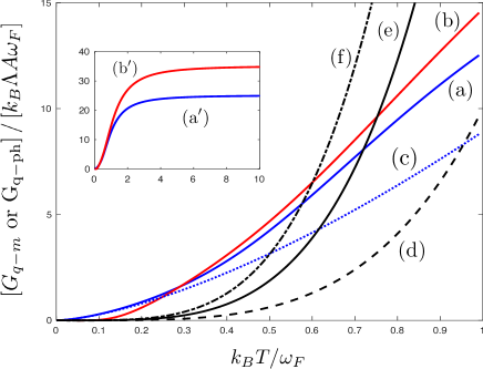
Figure 2: Electron-magnon $G_{\rm q-m}$ [Eqs. ((8)-(10)), curves (a)-(c) and (a’), (b’)] and electron-phonon heat conductance $G_{\rm q-ph}$ [Eq. (13), curves (d)-(f)] vs temperature $T$ for the thin film normal metal-ferromagnetic insulator hybrid structure. In (a) and (b) the chosen magnon band gap is $\omega_{0}=0$ and $\omega_{0}=0.8\omega_{F}$, respectively. Curve (c) is the analytical estimate of electron-magnon heat conductance from Eq. (12b), valid at $k_{B}T\ll\omega_{F}$ for the magnon band gap $\omega_{0}=0$. The curves $\mathrm{(a^{\prime})}$ and $\mathrm{(b^{\prime})}$ in the inset represent the corresponding extended plots of (a) and (b), respectively. Curves (d)-(f) show the electron-phonon heat conductance for three different thicknesses of the normal-metal film, for $d_{N}/d_{l}=2$, $d_{N}/d_{l}=6$ and $d_{N}/d_{l}=10$, respectively.

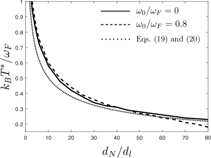
Figure 3: Temperature $T^{*}$ below which the electron-magnon thermalization dominates the electron-phonon mechanism, as a function of the thickness $d_{N}$ of the normal metal film. The curves are for two different values of the magnon band gap. The dotted line shows the analytical estimate from Eq. (19). The thickness is scaled by $d_{l}$ defined in Eq. (20).

$$k_{B}T^{*} = 1.26~{}\omega_{F}\left(d_{l}/d_{N}\right)^{2/5},$$ (19)

$$\mathrm{with}~{}d_{l} = k_{B}^{5}(\Lambda/\Sigma)\omega_{F}^{-3}$$ (20)

for $\omega_{0}=0$ and $k_{B}T^{*}<\omega_{F}$. This estimate works quite well even for a non-zero $\omega_{0}$, as shown in Fig. 3.

Let us also estimate typical values of parameters and the resulting $T^{*}$. In particular, we consider EuS/Al and EuO/Al hybrid structures, where EuS and EuO are ferromagnetic insulators, and Al is a metal. The Al characteristic electron-phonon coupling constant $\Sigma=0.2\times 10^{9}$ Wm^-3K^-5 Giazotto et al. (2006). Both EuS and EuO are characterized by the effective lattice spin $s=7/2$ Rohling et al. (2018), lattice constant $\zeta=5.1$ $\mathrm{\AA}$ Rohling et al. (2018) and the characteristic (Bloch-Grüneisen type) magnon frequency $\omega_{F}/k_{B}=T_{F}=53$ K Rohling et al. (2018). The interfacial coupling energy is around $J=10$ meV Rohling et al. (2018), for both hybrid structures, EuS/Al and EuO/Al, but its precise value depends on the quality of the contact. Using these values and $\mu=\hbar^{2}k_{F}^{2}/(2m_{e})$ with a free electron mass $m_{e}$, we get $\Lambda=7.5\times 10^{48}$ J^-1m^-2s^-1 and $d_{l}=50$ pm. As a result we get the crossover temperature $T^{*}=3$ K for both hybrid structures with the Al thickness of $100$ nm. Electron-magnon thermalization hence becomes relevant in modern-day low-temperature experiments on thin film bilayers.

III.2 Superconductor-ferromagnetic insulator structure

Because many functionalities of low-temperature devices Giazotto et al. (2006); Bergeret et al. (2018); Heikkilä et al. (2019) employ superconductivity, we also analyze the effect of superconductivity on the electron-magnon heat conduction. In this case two new energy scales show up: the superconducting energy gap $\Delta$ and the exchange field $h$ induced by the magnetic proximity effect into the superconductor Meservey and Tedrow (1994); Heikkilä et al. (2019). The latter might be present also in the normal state, but there it is not relevant to the magnitude of the heat conductance as long as it is much smaller than $\mu$.

Since the superconducting gap $\Delta(T,h)$ depends on $h$ and $T$, in what follows we introduce scaling energy as the magnitude of the gap $\Delta_{0}$ at $T=0$ K and $h=0$. We compute $\Delta(T,h)$ self-consistently using Eq. (33) (see Appendix C). Self-consistent calculation is significant near the critical magnetic field Chandrasekhar (1962); Clogston (1962), and near the critical temperature, but does not otherwise affect the results much. In Fig. 4 we plot again the two heat conductances $G_{\rm q-m}$ and $G_{\rm q-ph}$ in the case where the metal is in the superconducting state. As in the analytical estimates, Eqs. (15) and (17), both decay exponentially at low temperatures $k_{B}T\ll\Delta$ due to the exponential decay of the number of quasiparticles, $\sim\exp(-\Delta/k_{B}T)$. It is thus easier to compare their ratio, or the temperature $T^{*}$ at which they become equal. That temperature is plotted in Fig. 5. We can see that the overall behavior with respect to $d_{S}$ is quite similar to the normal state, but superconductivity affects the two processes slightly differently. In Figs. 4 and 5, we introduce a length scale

$$d_{\Delta}=k_{B}^{5}(\Lambda/\Sigma)\Delta_{0}^{-3},$$ (21)

associated with scaling energy $\Delta_{0}$. Note that in the usual case $\omega_{F}\gg\Delta$, $d_{\Delta}\gg d_{l}$ introduced in Eq. (20). In order to get the crossover temperature $T^{*}$ to be significantly below the superconducting critical temperature $T_{c}$, we would hence have to assume thicker films or smaller exchange couplings than those discussed in the previous section. Besides $\omega_{F}$ and $\Delta$, also the precise value of the magnon band gap affects $T^{*}$. However, we find that $T^{*}$ is slowly varying with the superconductor film thickness ($d_{S}$) irrespective of the small magnon band gap in Fig. 5.

In Sec. III.1, we find that an EuS/Al film with 100 nm Al layer can have a crossover temperature at 3 K, much above the Al $T_{c}$ (usually $1.2$ K in thin films in absence of spin-splitting field). Hence, to find the crossover in EuS/Al films in the superconducting state, the Al layer should be much thicker. Using the parameters of EuS/Al and EuO/Al as i n Sec. III.1 with $\Delta_{0}/k_{B}=2$ K Matthias et al. (1963), we get $d_{\Delta}=900$ nm. Hence $d_{S}=100$ nm would correspond to $T^{*}>T_{c}$, consistent with the normal-state estimate.

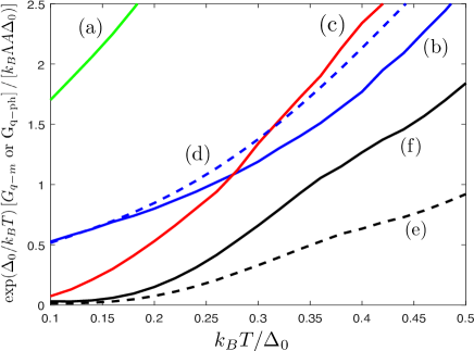
Figure 4: Electron-magnon $G_{\rm q-m}$ [Eqs. ((8), (9) and (14)), curves (a)-(d)] and electron-phonon heat conductance $G_{\rm q-ph}$ [Eqs. ((16a)-(16c)), curves (e)-(f)] vs temperature $T$ for the thin film superconductor-ferromagnetic insulator hybrid structure. The parameters for the curves are (a) $\omega_{0}=0$, $\omega_{F}=\Delta_{0}$ and (b) $\omega_{0}=0$, $\omega_{F}=10\Delta_{0}$ and (c) $\omega_{0}=0.5\Delta_{0}$, $\omega_{F}=10\Delta_{0}$. The curve (d) is the analytical estimate (Eq. (15)) of the electron-magnon heat conductance for the given parameters in (b) curve. The thin film superconductor thicknesses are in curve (e) $d_{S}/d_{\Delta}=0.4$ and (f) $d_{S}/d_{\Delta}=0.8$. For all the curves we set $h=0$ and $\Gamma=10^{-3}\Delta_{0}$.

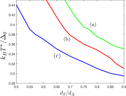
Figure 5: Crossover temperature $T^{*}$ below which electron-magnon thermalization becomes dominant, as a function of the thickness $d_{S}$ of the superconductor. For all curves we set $h=0$ and $\Gamma=10^{-3}\Delta_{0}$. The parameters for the curves are (a) $\omega_{0}=0$, $\omega_{F}=26\Delta_{0}$ (b) $\omega_{0}=0.5\Delta_{0}$, $\omega_{F}=50\Delta_{0}$ and (c) $\omega_{0}=0$, $\omega_{F}=50\Delta_{0}$.

Let us next study the effect of the induced spin-splitting field on the electron-magnon heat conductance. That is plotted in Fig. 6 at three different temperatures for a low value of the magnon gap $\omega_{0}$. Note that we here neglected the effect of spin relaxation, which may become especially relevant for higher $h$. Perhaps surprisingly, the effect of the spin splitting on $G_{\rm q-m}$ is quite modest, taking into account that the field reduces the energy gap from $\Delta$ to $\Delta-h$ for one of the spin species. However, since the electron-magnon coupling couples both spins, this reduced gap is not immediately visible.

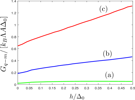
Figure 6: Electron-magnon heat conductance $G_{\rm q-m}$ vs spin-splitting field $h$ for the thin film superconductor-ferromagnetic insulator hybrid structure. For all curves $\omega_{0}=0.1\Delta_{0}$, $\omega_{F}=\Delta_{0}$ and $\Gamma=10^{-3}\Delta_{0}$. The curves (a), (b) and (c) are for $k_{B}T=0.2\Delta_{0}$, $k_{B}T=0.3\Delta_{0}$ and $k_{B}T=0.4\Delta_{0}$, respectively.

In the superconducting case, also the relation between the spin-splitting field and the magnon gap $\omega_{0}$ affects the magnitude of the electron-magnon heat conductance. This is shown in Fig. 7 showing $G_{\rm q-m}$ as a function $\omega_{0}$ for $h=0.1\Delta_{0}$. When $\omega_{0}\approx 2h$, $G_{\rm q-m}$ has a shallow maximum (a kink), as this is where the magnons just above the gap edge couple the electrons at the edges of the two spin bands (see Eq. (14)). However, due to the low density of states of the magnons at the gap edge, the dependence is not very strong. It might however be observable in the case where the spin-splitting field is tuned with an external magnetic field. Hence especially in the superconducting case the electron-magnon heat conductance can be used to obtain spectroscopic information about the magnons.

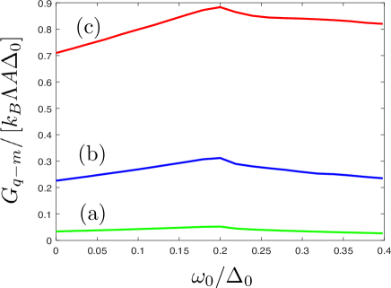
Figure 7: Electron-magnon heat conductance $G_{\rm q-m}$ vs magnon band gap $\omega_{0}$ for the thin film superconductor-ferromagnetic insulator hybrid structure. For all the curves $h=0.1\Delta_{0}$, $\omega_{F}=\Delta_{0}$ and $\Gamma=10^{-3}\Delta_{0}$. The curves (a), (b) and (c) are for $k_{B}T=0.2\Delta_{0}$, $k_{B}T=0.3\Delta_{0}$ and $k_{B}T=0.4\Delta_{0}$, respectively.

IV Conclusions

In this work we have studied heat transport between the electrons in a metallic thin film in a normal or a superconducting state and the magnons in a nearby ferromagnetic insulator film, resulting from the interfacial electron-magnon interaction. This mechanism can dominate over the electron-phonon heat transport at low temperatures and hence should be taken into account in device concepts Bergeret et al. (2018) utilizing such hybrid structures at low temperatures. The crossover temperature below which the electron-magnon process starts to dominate depends on the properties of the magnet and naturally on the electron-magnon interaction, but also on the thickness of the metal film. For reasonable values of the parameters of these films we find that this crossover temperature can be of the order of $1$ Kelvin. In this work we assume that the magnons flow away and only somewhere far from the interface thermalize with the phonons. In this situation the extra heat resistance related to this thermalization mechanism can be disregarded. Similarly, depending on the device geometry, one might have to include the (Kapitza) thermal boundary resistance for thermalizing the phonons, and this would affect the overall heat balance and the crossover temperatures. In the superconducting state, the magnitude of the induced spin-splitting field also affects the size of the heat conductance. In particular, the heat conductance obtains a maximum when the spin-splitting field equals half of the gap in the magnon spectrum. Because the spin-splitting field can be varied by using an external field (see, e.g., Xiong et al. (2011)), this dependence can be studied in detail. Such a study would hence reveal spectroscopic information about the magnon spectrum in the ferromagnetic insulator.

This project was supported by the Academy of Finland via its Key Funding project (Project No. 305256) and regular project number 317118 and from the European Union’s Horizon 2020 research and innovation programme under grant agreement No 800923 (SUPERTED).

Appendix A Discrete to continuous transformation

Here we demonstrate the discrete to continuous transformation for the case of the N-FI hybrid structure. For thin films $\vec{k}$ and ${\vec{q}}$ are two-dimensional, and hence we have the following discrete to continuous transformation

$$\sum_{\vec{k},\vec{q}}F(\epsilon_{\vec{k}},\omega_{\vec{q}})\delta(\epsilon_{\vec{k}+\vec{q}}-\epsilon_{\vec{k}}\pm\omega_{\vec{q}}\mp 2h) = \left(\frac{A}{4\pi^{2}}\right)^{2}\int d^{2}k~{}d^{2}q~{}F(\epsilon_{\vec{k}},\omega_{\vec{q}})\delta(\epsilon_{\vec{k}+\vec{q}}-\epsilon_{\vec{k}}\pm\omega_{\vec{q}}\mp 2h)$$ (22)

$$= \left(\frac{\pi k_{F}^{2}A^{2}}{32\pi^{4}B\mu}\right)\int_{0}^{\infty}d\epsilon_{\vec{k}}\int_{\omega_{0}}^{\infty}d\omega_{\vec{q}}\int_{0}^{2\pi}d\theta~{}F(\epsilon_{\vec{k}},\omega_{\vec{q}})\delta(\epsilon_{\vec{k}+\vec{q}}-\epsilon_{\vec{k}}\pm\omega_{\vec{q}}\mp 2h).~{}~{}~{}$$

To obtain Eq. (22) we have used the energy dispersion of the normal-metal electrons, $\epsilon_{\vec{k}}=\mu k^{2}/k_{F}^{2}$, and the energy dispersion of the magnons, $\omega_{\vec{q}}=\omega_{0}+Bq^{2}$. Therefore we have $kdk=k_{F}^{2}/(2\mu)d\epsilon_{\vec{k}}$ and $qdq=1/(2B)d\omega_{\vec{q}}$. We also have

$$\epsilon_{\vec{k}+\vec{q}}-\epsilon_{\vec{k}}\approx\hbar v_{F}\sqrt{\frac{\omega_{\vec{q}}-\omega_{0}}{B}}\cos\theta+\frac{\mu(\omega_{\vec{q}}-\omega_{0})}{Bk_{F}^{2}},$$ (23)

where $\theta$ is the angle between $\vec{k}$ and $\vec{q}$, and the Fermi energy $\mu$ is much larger than the relevant magnon energies $\omega_{\vec{q}}$. Here after integrating the Dirac delta function over $\theta$ in Eq. (22), we obtain the following result,

$$\int_{0}^{2\pi}d\theta~{}\delta(\epsilon_{\vec{k}+\vec{q}}-\epsilon_{\vec{k}}\pm\omega_{\vec{q}}\mp 2h)=\frac{1}{\mu}\sqrt{\frac{\omega_{F}}{\omega_{\vec{q}}-\omega_{0}}}\left|\mathrm{Re}\left[1-\frac{1}{4}\left(\frac{\omega_{\vec{q}}-\omega_{0}}{\omega_{F}}\right)\right]^{-1/2}\right|,$$ (24)

assuming the relevant magnons and the weak spin-splitting field satisfy $(\omega_{\vec{q}}\pm 2h)/\mu\rightarrow 0$. Equations (22)-(24) are used in Eqs. (5)-(10).

Next, we have followed the similar mathematical protocol in the case where the metal becomes superconducting. In this case $\left|{dE_{\vec{k}+\vec{q}}}/{d\theta}\right|=2\mu|\sin\theta|/N_{S}(E_{\vec{k}+\vec{q}})$ and $d\epsilon_{\vec{k}}=N_{S}\left(E_{\vec{k}}\right)dE_{\vec{k}}$, where $E_{\vec{k}}=\sqrt{\left(\epsilon_{\vec{k}}-\mu\right)^{2}+\Delta^{2}}$. Here $N_{S}$ is the superconducting density of states. After the discrete to continuous transformation and integrating the Dirac delta functions analogous to that above, we get the kernel terms $K^{(\pm)}$ in Eq. (14).

Appendix B Electron-magnon heat conductance of S-FI at low temperatures

In order to obtain the analytical expression of $G_{\rm q-m}$ of a S-FI hybrid structure we here consider $\omega_{0}=h=0$ and $k_{B}T<\Delta\ll 2\omega_{F}$, such that we can effectively have $4\omega_{F}/k_{B}T\rightarrow\infty$ and $\omega/4\omega_{F}\rightarrow 0$. Now using Eqs. (9) and (14) we have

$$G^{(\pm)}_{\rm q-m}=\pm\frac{k_{B}^{5/2}T^{3/2}}{8\sqrt{\omega_{F}}}\int_{0}^{\infty}dx\int_{0}^{\infty}dy~{}y^{3/2}\tilde{N}_{S}(x)\tilde{N}_{S}(x\mp y)$$

$$~{}~{}~{}~{}~{}~{}~{}~{}~{}~{}~{}\times\left[1+\Theta(x\mp y)\frac{\tilde{\Delta}^{2}}{xy}\right]F(x,y),$$ (25)

$$F(x,y)=\mathrm{cosech}\left(\frac{y}{2}\right)\mathrm{sech}\left(\frac{x}{2}\right)\mathrm{sech}\left(\frac{x\mp y}{2}\right),$$ (26)

where $\tilde{N}_{S}(x)=\lim_{\tilde{\Gamma}\rightarrow 0}\left|\mathrm{Re}\left[{(x+i\tilde{\Gamma})}/{\sqrt{(x+i\tilde{\Gamma})^{2}-\tilde{\Delta}^{2}}}\right]\right|$ and $\tilde{\Delta}=\Delta/k_{B}T$. The integrand in Eq. (25) is nonzero only for $x\geq\tilde{\Delta}$ and $x\mp y\geq\tilde{\Delta}$, hence at low temperatures we can approximate

$$\mathrm{sech}\left(\frac{x}{2}\right)\approx 2e^{-|x|/2},$$ (27)

$$\mathrm{sech}\left(\frac{x\mp y}{2}\right)\approx 2e^{-|x\mp y|/2}.$$ (28)

Combining Eqs. (25)-(28) we obtain

$$G^{(+)}_{\rm q-m}-G^{(-)}_{\rm q-m}=\frac{k_{B}^{5/2}T^{3/2}}{8\sqrt{\omega}_{F}}\int_{\tilde{\Delta}}^{\infty}dx\int_{\tilde{\Delta}}^{\infty}dy~{}\frac{xy+\tilde{\Delta}^{2}}{\sqrt{(x^{2}-\tilde{\Delta}^{2})(y^{2}-\tilde{\Delta}^{2})}}F_{1}(x,y)$$

$$~{}~{}~{}~{}~{}~{}~{}~{}~{}~{}~{}~{}~{}~{}~{}~{}~{}~{}~{}~{}~{}+\frac{k_{B}^{5/2}T^{3/2}}{8\sqrt{{\omega}_{F}}}\int_{\tilde{\Delta}}^{\infty}dx\int_{-\infty}^{-\tilde{\Delta}}dy~{}\tilde{N}_{S}(x)\tilde{N}_{S}(y)F_{1}(x,y),$$ (29)

$$F_{1}(x,y)=4|x-y|^{3/2}\mathrm{cosech}(|x-y|/2)e^{-|x|/2}e^{-|y|/2}.$$ (30)

The first term in the right hand side in Eq. (29) represents quasiparticle-magnon scattering, where as the second term is due to quasiparticle recombination processes. Now approximating $\sinh^{-1}\left(\frac{2\tilde{\Delta}+x+y}{2}\right)=2e^{-\tilde{\Delta}}e^{-(x+y)/2}$ for $x,y>0$, we finally have

$$G^{(+)}_{\rm q-m}-G^{-}_{\rm q-m}=\frac{k_{B}^{5/2}T^{3/2}}{\sqrt{{\omega}_{F}}}\left(\tilde{\Delta}e^{-\tilde{\Delta}}\sum_{n=0}^{\infty}\frac{D_{n}}{\tilde{\Delta}^{n}}+\tilde{\Delta}^{5/2}e^{-2\tilde{\Delta}}\sum_{n=0}^{\infty}\frac{E_{n}}{\tilde{\Delta}^{n}}\right),$$ (31)

$$\implies G_{\rm q-m}=\frac{k_{B}^{5/2}T^{3/2}\Lambda A}{\sqrt{{\omega}_{F}}}\left(\tilde{\Delta}e^{-\tilde{\Delta}}\sum_{n=0}^{\infty}\frac{D_{n}}{\tilde{\Delta}^{n}}+\tilde{\Delta}^{5/2}e^{-2\tilde{\Delta}}\sum_{n=0}^{\infty}\frac{E_{n}}{\tilde{\Delta}^{n}}\right),$$ (32)

with the lowest-order coefficients $D_{0}=4.82$, $D_{1}=2.88$, $E_{0}=\sqrt{2}\pi$, $E_{1}=\pi/\sqrt{2}$.

Appendix C Self-consistent equation for $\Delta(T,h)$

Neglecting spin relaxation effect, we have the self-consistent equation for the superconducting gap, $\Delta(T,h)$, as

$$\Delta=\frac{\lambda}{2}\int_{-\Omega_{D}}^{\Omega_{D}}d\epsilon\ \text{Im}\left[F_{01}(\epsilon)\right]\tanh\left(\frac{\epsilon}{2k_{B}T}\right),$$ (33)

where $\lambda$ is the effective coupling constant, $\Omega_{D}$ is the Debye cutoff energy and

$$F_{01}(\epsilon)=\frac{1}{2}\left[F_{0}(\epsilon+h)+F_{0}(\epsilon-h)\right],$$ (34)

$$F_{0}(\epsilon)=\frac{i\Delta}{\sqrt{(\epsilon+i\Gamma)^{2}-\Delta^{2}}}$$ (35)

with the Dynes parameter $\Gamma$. We use this self-consistent superconducting gap to compute various quantities in the main text of the paper.

References

- Irwin and Hilton (2005) K. Irwin and G. Hilton, “Transition-edge sensors,” in Cryogenic Particle Detection, edited by C. Enss (Springer Berlin Heidelberg, Berlin, Heidelberg, 2005) pp. 63–150.
- Grossman et al. (1991) E. N. Grossman, D. G. McDonald, and J. E. Sauvageau, IEEE Trans. Magn. 27, 2677 (1991).
- Bluzer and Forrester (1994) N. Bluzer and M. G. Forrester, Opt. Eng. 33, 33 (1994).
- Sergeev et al. (2002) A. V. Sergeev, V. V. Mitin, and B. S. Karasik, Appl. Phys. Lett. 80, 817 (2002).
- Giazotto et al. (2008) F. Giazotto, T. T. Heikkilä, G. P. Pepe, P. Helistö, A. Luukanen, and J. P. Pekola, Appl. Phys. Lett. 92, 162507 (2008).
- Govenius et al. (2016) J. Govenius, R. E. Lake, K. Y. Tan, and M. Möttönen, Phys. Rev. Lett. 117, 030802 (2016).
- Giazotto et al. (2006) F. Giazotto, T. T. Heikkilä, A. Luukanen, A. M. Savin, and J. P. Pekola, Rev. Mod. Phys. 78, 217 (2006).
- Heikkilä et al. (2018) T. T. Heikkilä, R. Ojajärvi, I. J. Maasilta, E. Strambini, F. Giazotto, and F. S. Bergeret, Phys. Rev. Applied 10, 034053 (2018).
- Chakraborty and Heikkilä (2018) S. Chakraborty and T. T. Heikkilä, J. Appl. Phys. 124, 123902 (2018).
- Kawabata et al. (2013) S. Kawabata, A. Ozaeta, A. S. Vasenko, F. W. J. Hekking, and F. Sebastian Bergeret, Appl. Phys. Lett. 103, 032602 (2013).
- Rouco et al. (2018) M. Rouco, T. T. Heikkilä, and F. S. Bergeret, Phys. Rev. B 97, 014529 (2018).
- Lian et al. (2018) B. Lian, X.-Q. Sun, A. Vaezi, X.-L. Qi, and S.-C. Zhang, PNAS 115, 10938 (2018).
- Wellstood et al. (1994) F. C. Wellstood, C. Urbina, and J. Clarke, Phys. Rev. B 49, 5942 (1994).
- Timofeev et al. (2009) A. V. Timofeev, C. P. García, N. B. Kopnin, A. M. Savin, M. Meschke, F. Giazotto, and J. P. Pekola, Phys. Rev. Lett. 102, 017003 (2009).
- Maisi et al. (2013) V. F. Maisi, S. V. Lotkhov, A. Kemppinen, A. Heimes, J. T. Muhonen, and J. P. Pekola, Phys. Rev. Lett. 111, 147001 (2013).
- Bergeret et al. (2018) F. S. Bergeret, M. Silaev, P. Virtanen, and T. T. Heikkilä, Rev. Mod. Phys. 90, 041001 (2018).
- Rohling et al. (2018) N. Rohling, E. L. Fjærbu, and A. Brataas, Phys. Rev. B 97, 115401 (2018).
- Bender et al. (2012) S. A. Bender, R. A. Duine, and Y. Tserkovnyak, Phys. Rev. Lett. 108, 246601 (2012).
- Takahashi et al. (2010) S. Takahashi, E. Saitoh, and S. Maekawa, Journal of Physics: Conference Series 200, 062030 (2010).
- Tserkovnyak et al. (2002) Y. Tserkovnyak, A. Brataas, and G. E. W. Bauer, Phys. Rev. B 66, 224403 (2002).
- Mahfouzi and Nikolić (2014) F. Mahfouzi and B. K. Nikolić, Phys. Rev. B 90, 045115 (2014).
- Cheng et al. (2017) Y. Cheng, K. Chen, and S. Zhang, Phys. Rev. B 96, 024449 (2017).
- Tveten et al. (2015) E. G. Tveten, A. Brataas, and Y. Tserkovnyak, Phys. Rev. B 92, 180412 (2015).
- Schreier et al. (2013) M. Schreier, A. Kamra, M. Weiler, J. Xiao, G. E. W. Bauer, R. Gross, and S. T. B. Goennenwein, Phys. Rev. B 88, 094410 (2013).
- Ozaeta et al. (2014) A. Ozaeta, P. Virtanen, F. S. Bergeret, and T. T. Heikkilä, Phys. Rev. Lett. 112, 057001 (2014).
- Machon et al. (2013) P. Machon, M. Eschrig, and W. Belzig, Phys. Rev. Lett. 110, 047002 (2013).
- Machon et al. (2014) P. Machon, M. Eschrig, and W. Belzig, New J. Phys. 16, 073002 (2014).
- Kolenda et al. (2016) S. Kolenda, M. J. Wolf, and D. Beckmann, Phys. Rev. Lett. 116, 097001 (2016).
- Kolenda et al. (2017) S. Kolenda, C. Sürgers, G. Fischer, and D. Beckmann, Phys. Rev. B 95, 224505 (2017).
- Rezaei et al. (2018) A. Rezaei, A. Kamra, P. Machon, and W. Belzig, New J. Phys. 20, 073034 (2018).
- Giazotto et al. (2014) F. Giazotto, J. Robinson, J. Moodera, and F. Bergeret, Appl. Phys. Lett. 105, 062602 (2014).
- Giazotto et al. (2015) F. Giazotto, T. T. Heikkilä, and F. S. Bergeret, Phys. Rev. Lett. 114, 067001 (2015).
- Van Kranendonk and Van Vleck (1958) J. Van Kranendonk and J. H. Van Vleck, Rev. Mod. Phys. 30, 1 (1958).
- Kubo (1957) R. Kubo, J. Phys. Soc. Japan 12, 570 (1957).
- Dynes et al. (1984) R. C. Dynes, J. P. Garno, G. B. Hertel, and T. P. Orlando, Phys. Rev. Lett. 53, 2437 (1984).
- Heikkilä et al. (2019) T. T. Heikkilä, M. Silaev, P. Virtanen, and F. S. Bergeret, arXiv:1902.09297 (2019).
- Meservey and Tedrow (1994) R. Meservey and P. Tedrow, Phys. Rep. 238, 173 (1994).
- Chandrasekhar (1962) B. S. Chandrasekhar, Appl. Phys. Lett. 1, 7 (1962).
- Clogston (1962) A. M. Clogston, Phys. Rev. Lett. 9, 266 (1962).
- Matthias et al. (1963) B. T. Matthias, T. H. Geballe, and V. B. Compton, Rev. Mod. Phys. 35, 1 (1963).
- Xiong et al. (2011) Y. M. Xiong, S. Stadler, P. W. Adams, and G. Catelani, Phys. Rev. Lett. 106, 247001 (2011).