Analysis of beam position monitor requirements with Bayesian Gaussian regression

Abstract

With a Bayesian Gaussian regression approach, a systematic method for analyzing a storage ring’s beam position monitor (BPM) system requirements has been developed. The ultimate performance of a ring-based accelerator, based on brightness or luminosity, is determined not only by global parameters, but also by local beam properties at some particular points of interest (POI). BPMs used for monitoring the beam properties, however, cannot be located at these points. Therefore, the underlying and fundamental purpose of a BPM system is to predict whether the beam properties at POIs reach their desired values. The prediction process can be viewed as a regression problem with BPM readings as the training data, but containing random noise. A Bayesian Gaussian regression approach can determine the probability distribution of the predictive errors, which can be used to conversely analyze the BPM system requirements. This approach is demonstrated by using turn-by-turn data to reconstruct a linear optics model, and predict the brightness degradation for a ring-based light source. The quality of BPMs was found to be more important than their quantity in mitigating predictive errors.

I introduction

The ultimate performance of a ring-based accelerator is determined not only by certain critical global parameters, such as beam emittance, but also by local properties of the beam at particular points of interest (POI). The capability of diagnosing and controlling local beam parameters at POIs, such as beam size and divergence, is crucial for a machine to achieve its design performance. Examples of POIs in a dedicated synchrotron light source ring include the undulator locations, from where high brightness X-rays are generated. In a collider, POIs are reserved for detectors in which the beam-beam luminosity is observed. However, beam diagnostics elements, such as beam position monitors (BPM) are generally placed outside of the POIs as the POIs are already occupied. An intuitive, but quantitatively unproven belief, is that the desired beam properties at the POIs can be achieved once the beam properties are well-controlled at the location of the BPMs.

Using observational data at BPMs to indirectly predict the beam properties at POIs can be viewed as a regression problem and can be treated as a supervised learning process: BPM readings at given locations are used as a training dataset. Then a ring optics model with a set of quadrupole excitations as its arguments is selected as the hypothesis. From the dataset, an optics model needs to be generalized first. Based on the model, the unknown beam properties at POIs can be predicted. However, there exists some systematic error and random uncertainty in the BPMs’ readings, and the quantity of BPMs (the dimension of the training dataset) is limited. Therefore, the parameters in the reconstructed optics model have inherent uncertainties, as do the final beam property predictions at the POIs. The precision and accuracy of the predictions at the POIs depend on the quantity of BPMs, their physical distribution pattern around the ring, and their calibration, resolution, etc. When a BPM system is designed for a storage ring, however, it is more important to consider the inverse problem: i.e. How are the BPM system technical requirements determined in order to observe whether the ring achieves its desired performance? In this paper, we developed an approach to address this question with Bayesian Gaussian regression.

In statistics, a Bayesian Gaussian regression Rasmussen and Williams (2006); Bishop (2006) is a Bayesian approach to multivariate regression, i.e. regression where the predicted outcome is a vector of correlated random variables rather than a single scalar random variable. Every finite collection of the data has a normal distribution. The distribution of generalized arguments of the hypothesis is the joint distribution of all those random variables. Based on the hypothesis, a prediction can be made for any unknown dataset within a continuous domain. In our case, multiple BPMs’ readings are normally distributed around their real values. The standard deviations of the Gaussian distributions are BPM’s resolutions. A vector composed of quadrupoles’ mis-settings is the argument to be generalized. The prediction at the POIs is the function of this vector. The continuous domain is the longitudinal coordinate $s$ along a storage ring.

To further explain this approach, the remaining sections are outlined as follows: Sect. II introduces the relation between machine performance and beam diagnostics system capabilities. Sect. III explains the procedure of applying the Bayesian Gaussian regression in the ring optics model reconstruction, and the prediction of local optics properties at POIs. In Sect. IV, the National Synchrotron Light Source II (NSLS-II) storage ring and its BPM system are used to illustrate the application of this approach. Some discussions and a brief summary is given in Sect. V.

II machine performance and beam diagnostics capability

As mentioned previously, ultimate performance of a ring-based accelerator relies heavily on local beam properties at particular POIs. Consider a dedicated light source ring. Its ultimate performance is measured by the brightness of the X-rays generated by undulators. The brightness of undulator emission is determined by the transverse size of both the electron and photon beam and their angular divergence at their source points Lindberg and Kim (2015); Walker (2019); Chubar and Elleaume (1998); Hidas (2017). Therefore, the undulator brightness performance $\mathcal{B}$ depends on the ring’s global emittance and the local transverse optics parameters,

$$\mathcal{B} \propto \frac{1}{\Sigma_{x}\Sigma_{x}^{\prime}\Sigma_{y}\Sigma_{y}^{\prime}}$$

$$\Sigma_{x,y} = \sqrt{\epsilon_{x,y}\beta_{x,y}+\eta_{x,y}^{2}\sigma_{\delta}^{2}+\sigma^{2}_{ph}}$$

$$\Sigma_{x,y}^{\prime} = \sqrt{\epsilon_{x,y}\gamma_{x,y}+\eta_{x,y}^{\prime 2}\sigma_{\delta}^{2}+\sigma^{\prime 2}_{ph}}.$$ (1)

Here $\epsilon_{x,y}$ are the electron beam emittances, which represent the equilibrium between the quantum excitation and the radiation damping around the whole ring. $\beta,\gamma$ are the Twiss parameters Courant and Snyder (1958), $\eta,\eta^{\prime}$ are the dispersion and its derivative at the undulators’ locations, $\sigma_{\delta}$ is the electron beam energy spread $\sigma_{ph}=\frac{\sqrt{\lambda L_{u}}}{2\pi}$ and $\sigma^{\prime}_{ph}=\frac{1}{2}\sqrt{\frac{\lambda}{L_{u}}}$ are the X-ray beam diffraction “waist size” and its natural angular divergence, respectively. The X-ray wavelength $\lambda$, is determined based on the requirements of the beam-line experiments, and $L_{u}$ is the undulator periodic length. The emittance was found to be nearly constant with small $\beta$-beat (see Sect. IV). Therefore, monitoring and controlling the local POI’s Twiss parameters is crucial.

The final goal of beam diagnostics is to provide sufficient, accurate observations to reconstruct an online accelerator model. Modern BPM electronics can provide the beam turn-by-turn (TbT) data, which is widely used for the beam optics characterization and the model reconstruction. Based on the model, we can predict the beam properties not only at the locations of monitors themselves, but more importantly at the POIs. The capability of indirect prediction of the Twiss parameters at POIs eventually defines the BPM system requirements on TbT data acquisition. Based on Eq. (1), how precisely one can predict the bias and the uncertainty of Twiss parameters $\beta$ and $\eta$ at locations of undulators is the key problem in designing a BPM system. Therefore, to specify the technical requirements of a BPM system, the following questions need to be addressed: in order to make an accurate and precise prediction of beam properties at POIs, how many BPMs are needed? How should the BPMs be allocated throughout the accelerator ring, and how precise should the BPM TbT reading be?

In the following section a method of reconstructing the linear optics model, and determining the brightness performance for a ring-based light source will be discussed. For a collider ring, its luminosity is determined only by the beam sizes at the interaction points Herr and Muratori (2003). Gaussian regression analysis can therefore be applied to predict its $\beta^{*}$ and luminosity as well.

III Gaussian regression for model reconstruction and prediction

When circulating beam in a storage ring is disturbed, a BPM system can provide its TbT data at multiple longitudinal locations. TbT data of the BPMs can be represented as an optics model plus some random reading errors,

$$x(s)_{i}=A(i)\sqrt{\beta(s)}\cos\left[i\cdot 2\pi\nu+\phi(s)\right]+\varepsilon(s)_{i},$$ (2)

here $i$ is the index of turns, $A(i)$ is a variable dependent on turn number, $\beta(s)$ is the envelope function of Twiss parameters at $s$ location, $\nu$ is the betatron tune, $\phi$ is the betatron phase, and $\varepsilon(s)_{i}$ is the BPM reading noise Calaga and Tomás (2004); Langner et al. (2016); Cohen-Solal (2010), which generally has a normal distribution. Based on the accelerator optics model defined in Eq. (2), we can extract a set of optics Twiss parameters at all BPM locations Castro-Garcia (1996); Irwin et al. (1999); Huang et al. (2005); Tomás et al. (2017). Recently, Ref. Hao et al. (2019) proposed using a Bayesian approach to infer the mean (aka expectation) and uncertainty of Twiss parameters at BPMs simultaneously. The mean values of $\beta$ represent the most likely optics pattern. The random BPM reading error and the simplification of the optics model can result in some uncertainties, $\varepsilon_{\beta}$, in the inference process,

$$\beta=\beta(s,\boldsymbol{K})+\varepsilon_{\beta}(s),$$ (3)

here $\boldsymbol{K}$ is a vector composed of all normalized quadrupole focusing strengths, and $\varepsilon_{\beta}$ is the inference uncertainty. Unless otherwise stated, bold symbols, such as “$\boldsymbol{X}$”, are used to denote vectors and matrices throughout this paper. In accelerator physics, the deviation from the design model $\beta_{0}$ is often referred to as the $\beta$-beat. From the point of view of model reconstruction, the $\beta$-beat is due to quadrupole excitation errors and can be determined by

$$\Delta\beta=\beta(s,\boldsymbol{K}_{0}+\Delta\boldsymbol{K})-\beta_{0}(s,\boldsymbol{K}_{0})\approx\boldsymbol{M}\Delta\boldsymbol{K},$$ (4)

where $\boldsymbol{K}_{0}$ represents the quadrupoles’ nominal setting and $\beta_{0}$ is the nominal envelope function along $s$. $\boldsymbol{M}$ is the response matrix composed of elements $M_{i,j}=\frac{\partial\beta_{s_{i}}}{\partial K_{j}}$ observed by the BPMs. The dependency of $\beta$ on $\boldsymbol{K}$ is not linear in a complete optics model. However, when quadrupole errors are small enough, the dependence can be approximated as a linear relation as illustrated in Fig. 1. The approximation holds for most operational storage rings, and other diffraction limited light sources under design or construction. A linear approximation allows us to use the linear regression approach for this process. Eq. (3) or (4) is a hypothesis with the unknown arguments $\boldsymbol{K}$ or $\Delta\boldsymbol{K}$, which need to be generalized from BPM measurement data.

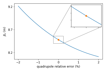
Figure 1: $\beta_{x}$ dependency on the excitation error of a quadrupole observed by a BPM at the NSLS-II ring. The dependency is nonlinear. However, when the quadrupole error is confined to a small range $[-0.25\%,0.25\%]$, it can be approximated as a linear dependence as shown in the zoomed-in window. At modern storage rings, such as NSLS-II, quadrupole excitation errors due to a power supply’s mis-calibration and/or magnetic hysteresis are much less than 0.25%.

Given a set of measured optics parameters $\beta$s at multiple locations $s$ from BPM TbT data, the posterior probability of the quadrupole error distribution $p(\Delta\boldsymbol{K}|\boldsymbol{\beta})$ can be given according to Bayes theorem Li et al. (2019),

$$p(\Delta\boldsymbol{K}|\boldsymbol{\beta}) = \frac{p(\boldsymbol{\beta}|\Delta\boldsymbol{K})p(\Delta\boldsymbol{K})}{p(\boldsymbol{\beta})}$$ (5)

$$\propto p(\boldsymbol{\beta}|\Delta\boldsymbol{K})p(\Delta\boldsymbol{K}).$$

Here $p(\boldsymbol{\beta}|\Delta\boldsymbol{K})$ is referred to as the likelihood function,

$$\mathcal{N}(\boldsymbol{\beta}|\bar{\boldsymbol{\beta}},\sigma_{\beta}^{2}) = \frac{1}{\sqrt{2\pi}\sigma_{\beta}}\exp\left[-\frac{(\boldsymbol{\beta}-\bar{\boldsymbol{\beta}})^{2}}{2\sigma_{\beta}^{2}}\right]$$ (6)

$$\approx \frac{1}{\sqrt{2\pi}\sigma_{\beta}}\exp\left[-\frac{(\Delta\boldsymbol{\beta}-\boldsymbol{M}\Delta\boldsymbol{K})^{2}}{2\sigma_{\beta}^{2}}\right].$$

Here $\bar{\beta}=\mathbb{E}(\beta)$ and $\sigma^{2}_{\beta}$ are the expectation value and the variance of the normal distribution of measured $\beta$s. Once the expectation value of the optics measurement is extracted from the TbT data, a prior quadrupole excitation error distribution $p(\Delta\boldsymbol{K})$ can be determined by comparing them against the design optics model,

$$p(\Delta\boldsymbol{K}) = \mathcal{N}(\Delta\boldsymbol{K}|0,\sigma_{\Delta K}^{2})$$ (7)

$$= \frac{1}{\sqrt{2\pi}\sigma_{\Delta K}}\exp\left[-\frac{\Delta\boldsymbol{K}^{2}}{2\sigma^{2}_{\Delta K}}\right],$$

in which the variance $\sigma^{2}_{\Delta K}$ of the prior distribution $p(\Delta\boldsymbol{K})$ is linearly proportional to the mean value of the measured $\beta$-beat,

$$\sigma_{\Delta K}\sim\kappa|\Delta\beta|=\kappa|\bar{\beta}-\beta_{0}|.$$ (8)

Here “$\sim$” in Eq. (8) describes a statistically proportional relationship between $\beta$-beats (in the unit of “m”) and quadrupole strength error $\Delta K$ (in units of $m^{-2}$). The coefficient $\kappa$ can be computed based on the optics model either analytically or numerically before carrying out any measurements. In the NSLS-II ring, $\kappa\approx 1.6\times 10^{-3}m^{-3}$, i.e. a $0.25m$ $\beta$-beat ($\frac{\Delta\beta}{\beta}\approx 1\%$) corresponds to a distribution of quadrupole errors with the standard deviation $4\times 10^{-4}m^{-2}$ ($\frac{\Delta K}{K}\approx 0.12\%$) as shown in Fig. 1 in Ref.  Li et al. (2019). Qualitatively, the relative $\beta$-beat and quadrupole error, i.e. $\frac{\Delta\beta}{\beta}$ and $\frac{\Delta K}{K}$ are often used in accelerator literature. Here the absolute $\Delta\beta$ and $\Delta K$ are used simply because they were adapted to our quantitative implementation.

Both the likelihood function and the prior distribution are generally normally distributed. Therefore, the posterior distribution is a normal distribution by summing over the arguments of the exponentials in Eq. (6) and (7),

$$(\Delta\boldsymbol{\beta}-\boldsymbol{M}\Delta\boldsymbol{K})^{T}\boldsymbol{S}_{\beta}^{-1}(\Delta\boldsymbol{\beta}-\boldsymbol{M}\Delta\boldsymbol{K})+\Delta\boldsymbol{K}^{T}\boldsymbol{S}_{K}^{-1}\Delta\boldsymbol{K}.$$ (9)

Here

$$\boldsymbol{S}_{\beta}^{-1}=\frac{1}{\sigma_{\beta}^{2}}\boldsymbol{I},\;\;\boldsymbol{S}_{K}^{-1}=\frac{1}{\sigma_{\Delta K}^{2}}\boldsymbol{I}.$$ (10)

The identity matrix $\boldsymbol{I}$ is used in Eq. (10) because all BPMs’ resolutions are assumed to have the same values $\sigma_{\beta}$. In reality, however, $\boldsymbol{S}_{\beta}^{-1}$ needs to be replaced with a diagonal matrix with different elements if the BPMs’ resolutions are different. The quadrupoles’ error distribution matrix $\boldsymbol{S}_{K}^{-1}$ needs to be processed in the same way if necessary. The mean value of the posterior, corresponding to the most likely quadrupole error distribution, can be used to implement the linear optics correction as explained in Ref. Li et al. (2019),

$$\boldsymbol{m}=\sigma^{-2}_{\beta}\boldsymbol{A}^{-1}\boldsymbol{M}^{T}\Delta\boldsymbol{\bar{\beta}},$$ (11)

where $\boldsymbol{A}=\left[\sigma^{-2}_{\beta}\boldsymbol{M}^{T}\boldsymbol{M}+\sigma^{-2}_{\Delta K}\boldsymbol{I}\right]$. Adding an extra term $\sigma^{-2}_{\Delta K}\boldsymbol{I}$ to prevent overfitting is known as the regularization technique. The posterior variance represents the uncertainty of quadrupole errors.

$$\boldsymbol{\Sigma_{K}^{2}}=\boldsymbol{A}^{-1}.$$ (12)

Given $\beta$-beats observed at $s$, the posterior generalizes an optics model, in which the quadrupoles errors are normally distributed,

$$p(\Delta\boldsymbol{K}|\Delta\boldsymbol{\beta},s)=\mathcal{N}(\Delta\boldsymbol{K}|\boldsymbol{m},\boldsymbol{\Sigma_{K}^{2}}),$$ (13)

with the mean value and the variance given by Eq. (11) and (12) respectively.

Thus far, the optics are measured at the locations of the BPMs, and the corresponding quadrupole error distributions are generalized based on the measurements. To confirm the machine brightness performance, we need to predict the beam properties at POIs. To do so, the output of all possible posterior quadrupole error distributions must be averaged,

$$p(\Delta\boldsymbol{\beta}_{*}|\boldsymbol{s}_{*},\Delta\boldsymbol{\beta},\boldsymbol{s}) = \int p(\Delta\boldsymbol{\beta}_{*}|\boldsymbol{s}_{*},\Delta\boldsymbol{K})p(\Delta\boldsymbol{K}|\Delta\boldsymbol{\beta},\boldsymbol{s})\mathrm{d}\boldsymbol{K}$$ (14)

$$= \mathcal{N}(\boldsymbol{m}_{*},\boldsymbol{\Sigma}_{*}^{2}).$$

Here $\Delta\boldsymbol{\beta}_{*}$ is the predicted result at POIs’ locations $\boldsymbol{s}_{*}$ given the measured $\Delta\boldsymbol{\beta}$ at $\boldsymbol{s}$. The mean values and the variances of the predicted distributions at POIs are

$$\boldsymbol{m}_{*} = \sigma^{-2}_{\beta}\boldsymbol{M}_{*}\boldsymbol{A}^{-1}\boldsymbol{M}^{T}\Delta\boldsymbol{\bar{\beta}}$$

$$\boldsymbol{\Sigma}_{*}^{2} = \boldsymbol{M}_{*}\boldsymbol{A}^{-1}\boldsymbol{M}^{T}_{*},$$ (15)

$\boldsymbol{M}_{*}$ is the Jacobian matrix of the optics response to quadrupole errors observed at POIs. The difference between the mean value $\boldsymbol{m}_{x}$ and the real $\beta$ at a POI is referred to as the predicted bias. By substituting the bias and uncertainty back into Eq. (1), we can estimate how accurate the brightness could be measured for given BPMs’ resolutions. Based on the desired brightness resolution, we can determine the needed quantity and resolution of BPMs.

IV Application to NSLS-II ring

In this section, we use the NSLS-II ring and its BPM system TbT data acquisition functionality to demonstrate the application of this approach. NSLS-II is a $3^{rd}$ generation dedicated light source. All undulator source points (POIs) are located at non-dispersive straights. Typical photon energy from undulators is around 10 $keV$, with corresponding wavelengths around 0.124 $nm$. The undulators’ period length is 20 $mm$. The horizontal beam emittance is 0.9 $nm\cdot rad$ including the contribution from 3 damping wigglers. The emittance coupling ratio can be controlled to less than 1%. At its 15 short straight centers, the Twiss parameters are designed to be as low as $\beta_{x,y}=1.80,\,1.20\,m$, and $\alpha_{x,y}=0$ to generate the desired high brightness x-ray beam from the undulators.

The horizontal emittance growth with an optics distortion was studied by carrying out a lattice simulation. With $\beta$-beat at a few percent, the corresponding $\alpha-$ and $\gamma$-distortions were generated by adding some normally distributed quadrupole errors based on Eq. (7) and (8). The horizontal emittance was found to grow slightly with the average $\beta$-beats as illustrated in Fig. 2. When there is about a 1% horizontal $\beta$-beat ($\sim 0.14m$), the emittance increases by only about 0.1%, which is negligible. Therefore, in the following calculation, the emittance was represented as a constant.

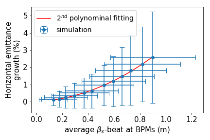
Figure 2: Beam horizontal emittance growth with the average $\beta_{x}$-beat for the NSLS-II ring. If the global $\beta_{x}$-beat can be controlled within 1%($\sim 0.15m$), the emittance growth is negligible.

Degradation of an undulatorís brightness is determined by its local optics distortion which can be evaluated with Eq. (1). Multi-pairs of simulated $\beta-\alpha$ were incorporated into the previously specified undulator parameters to observe the dependence of the X-ray brightness on the $\beta$-beat (see Fig. 3). A change of approximately 1% of the $\beta_{x,y}$ in the transverse plane can degrade the brightness by about 1%. In other words, in order to resolve a 1% brightness degradation, the predictive errors of the ring optics (including the bias and uncertainty) at the locations of undulators should be less than 1%. Because multiple undulators are installed around the ring, the predicted performance needs to be evaluated at all POIs simultaneously.

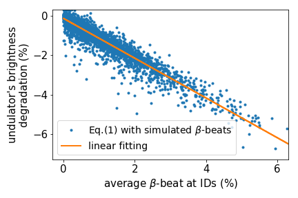
Figure 3: Brightness degradation of an undulator at a low-$\beta$ straight due to the average $\beta$-beats in the horizontal and vertical planes. Each dot represents a set of simulated optics distortions. The brightness degradation has an approximate linear dependence on $\beta$-beat.

There exist two types of errors in Eq. (2) which can introduce uncertainties in characterizing the optics parameters at BPMs. First, due to radiation damping, chromatic decoherence and nonlinearity, a disturbed bunched-beam trajectory is not a pure linear undamping betatron oscillation Meller et al. (1987). A reduced model (for example, assuming $A$ is a constant), will introduce systematic errors Malina et al. (2017); Carlà et al. (2016); Franchi et al. (2014); Langner et al. (2016). The second error source is the BPM TbT resolution limit, which results in random noise. At NSLS-II, the BPM TbT resolution at low beam current ($<2\;mA$) is inferred as $\sim 10-15\;\mu m$. When a $2^{nd}$ order polynomial function is used to represent the turn-dependent amplitude $A(i)$, the inferred $\beta$ function resolution at BPMs can be reached as low as 0.5% Hao et al. (2019).

First we studied the dependence of predictive errors on the quantity of BPMs. A comprehensive simulation was set up to compare the Gaussian regression predictive errors with the real errors. A linear optics simulation code was used to simulate the distorted optics due to a set of quadrupole errors. The $\beta$-beats observed at the BPMs were marked as the “real” values. On top of the real values, 0.5% random errors were added to simulate one-time measurement uncertainty seen by the BPMs. A posterior distribution Eq. (11) and (12) of the quadrupole errors was obtained by reconstructing the optics model with the likelihood function Eq. (6), and the prior distribution (7) and (8). The predicted optics parameters with their uncertainties were then calculated based on another likelihood function between quadrupoles and the locations of undulators with Eq. (14).

The results of comparison are illustrated in Fig.4. As with any regression problem, the training data distribution (i.e. the BPM locations) should be as uniform as possible within the continuous $s$ domain. There are 30 cells in the NSLS-II ring, and each cell has 6 BPMs. Equal numbers of BPMs were selected from each cell to make the training data uniformly distributed. The goal was to predict all straight section optics simultaneously. The predicted performance was therefore evaluated by averaging at multiple straight centers. Initially, one BPM was selected per cell. The number of selected BPMs was then gradually increased to observe the evolution of predictive errors. It was found that utilizing more BPMs improved the predicted performance, as expected. Both the bias and uncertainty were reduced with the quantity of BPMs. However, the improvement became less and less apparent once more than 4 BPMs per cell were used.

Since there are 6 BPMs per cell at the NSLS-II ring, we chose different BPM combinations. We found that some patterns/combinations of BPMs were better used to capture/measure these types of optics distortions. For example, each end of the straight sections needs one BPM to observe the ID, and at least one BPM needs to be located inside the achromat arc in order to observe the dipoles. The distribution of the BPMs does not need to be uniform in the longitudinal $s$ direction, instead, they should be uniform along the betatron phase propagation. Collider rings would see this effect more clearly due to the existence of interaction points. However, for most light source rings, including the NSLS-II ring, the phase propagation along the longitudinal direction is mostly quite linear in the longitudinal direction.

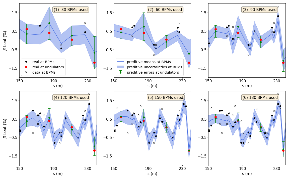
Figure 4: A zoomed-in view of predicted means and variances of $\beta$ observed at both BPMs (the training set) and undulators (POIs) for a section (spanning 3 cells, 4 POIs) of the NSLS-II ring. Black and red dots represent the real $\beta$ values at BPMs and POIs. Black crosses are the data observed by the BPMs. The light blue lines with a shadow are the predictions at the BPMs, and the green error bars are the final prediction at POIs. From subplot 1 to 6, the quantity of BPMs used increases gradually. A large set of training data (i.e. using more BPMs) for the regression does improve the accuracy and precision of the predicted results at POIs. However, the improvement becomes less apparent after using more than 120 BPMs.

Next, we studied the effect of $\beta$ measurement resolution on the predictive errors. A similar analysis was carried out but with different $\beta$-resolution as illustrated in Fig. 5. By observing Fig. 5, several conclusions can be drawn: (1) The degradation of the $\beta$ resolution reduced the accuracy of the generalized optics model. However, this can be improved by applying a more complicated optics model Hao et al. (2019). Thus, the BPM TbT resolution is the final limit on the resolution of $\beta$ parameters. In order to accurately and precisely predict the beam properties at POIs, improving the resolution of BPMs is crucial. (2) After a certain point, the predicted performance is not improved significantly with the quantity of BPMs as seen in both Fig 4 and 5. The advantage of reduction of predictive errors will gradually level out once enough BPMs are used. Meaning that quantitatively, the improvement in error reduction will eventually become negligible compared to the cost of adding more BPMs. The higher the resolution each individual BPM has, the less number of BPMs are needed. There should be a compromise between the required quality and quantity of BPMs to achieve an expected predictive accuracy. (3) The quality (resolution) is much more important than the quantity of BPMs from the point of view of optics characterization. For example, at NSLS-II, in order to resolve 1% brightness degradation, at least 120 BPMs with a $\beta$ resolution better than 1% are needed, or 90 BPMs with a 0.75% resolution, etc. Having more BPMs than is needed creates no obvious, significant improvement. Having 60 high precision (0.5% $\beta$-resolution) BPMs yields a better performance than having 180 low precision (1%) BPMs in this example.

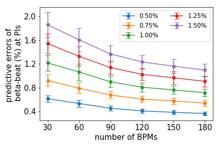
Figure 5: Predictive $\beta$-beat errors (including bias and uncertainties) at the locations of undulator (POIs). $\beta$s are observed with different number of BPMs and different resolutions. The resolution of $\beta$ is the final limit on predictive errors. The higher the resolution each individual BPM has, the less number of BPMs are needed.

V Discussion and summary

A systematic approach has been proposed to analyze a BPM systemís technical requirements in this manuscript. The approach is based on the resolution requirements for monitoring a machine’s ultimate performance. The Bayesian Gaussian regression is useful in statistical data modelling, such as reconstructing a ring’s optics model from beam TbT data. The optics properties of the ring are contained in a collection of data having a normal distribution. From past experience in designing and commissioning various accelerators, many will intuitively realize that having more BPMs does not always significantly improve diagnostics performance and is therefore not necessarily cost-effective for an accelerator design. Using the Gaussian regression method, however, confirmed that quantitatively. More importantly, a reasonable compromise can be reached between the quality (resolution) and the quantity of BPMs using this method.

It is worth noting that our approach is simplified as a linear regression by assuming a known linear dependence of optics distortion on quadrupole errors. If a ring’s optics are significantly different from the design model, this assumption is not valid. In our case, we needed to iteratively calculate the likelihood function $\boldsymbol{M}$ by incorporating the posterior mean of quadrupole errors Eq. (11) and compare it to the optics model until the best convergence was reached. This was not discussed in this paper, however, because our analysis applies best to machines whose optics are quite close to their design model. Other important effects on X-ray brightness, such as quadrupolar errors from sextupole feed down, skew quadrupoles, longitudinal misalignments of quadrupoles and BPMs, systematic gain errors in BPMs, magnet fringe field etc. are not addressed in detail here. These effects are neglected at the NSLS-II ring because either they are small compared with the quadrupole excitation errors and hysteresis, or their effects have been integrated into our optics model. The Gaussian regression method outlined here, however, can be expanded to take them into account if necessary.

In a ring-based accelerator, BPMs are used for multiple other purposes, such as orbit monitoring and optics characterization, etc. In this paper we only concentrated on a particular use case of TbT data to characterize the linear optics, and then to predict X-ray beam brightness performance. A similar analysis can be applied to the orbit stability, and dynamic aperture reduction due to $\beta$-beat as well. An accelerator’s BPM system needs to satisfy several objectives simultaneously. Therefore the Gaussian regression approach could/should be extended to a higher dimension parameter space to achieve an optimal compromise among these objectives.