Deep Back-Projection Networks for Single Image Super-resolution

Abstract

Previous feed-forward architectures of recently proposed deep super-resolution networks learn the features of low-resolution inputs and the non-linear mapping from those to a high-resolution output. However, this approach does not fully address the mutual dependencies of low- and high-resolution images. We propose Deep Back-Projection Networks (DBPN), the winner of two image super-resolution challenges (NTIRE2018 and PIRM2018), that exploit iterative up- and down-sampling layers. These layers are formed as a unit providing an error feedback mechanism for projection errors. We construct mutually-connected up- and down-sampling units each of which represents different types of low- and high-resolution components. We also show that extending this idea to demonstrate a new insight towards more efficient network design substantially, such as parameter sharing on the projection module and transition layer on projection step. The experimental results yield superior results and in particular establishing new state-of-the-art results across multiple data sets, especially for large scaling factors such as $8\times$.

1 Introduction

Significant progress in deep neural network (DNN) for vision [1, 2, 3, 4, 5, 6, 7] has recently been propagating to the field of super-resolution (SR) [8, 9, 10, 11, 12, 13, 14, 15, 16].

Single image SR (SISR) is an ill-posed inverse problem where the aim is to recover a high-resolution (HR) image from a low-resolution (LR) image. A currently typical approach is to construct an HR image by learning non-linear LR-to-HR mapping, implemented as a DNN [17, 18, 19, 13, 12, 20, 14] and non DNN [21, 22, 23, 24]. For DNN approach, the networks compute a sequence of feature maps from the LR image, culminating with one or more upsampling layers to increase resolution and finally construct the HR image. In contrast to this purely feed-forward approach, the human visual system is believed to use a feedback connection to simply guide the task for the relevant results [25, 26, 27]. Perhaps hampered by lack of such feedback, the current SR networks with only feed-forward connections have difficulty in representing the LR-to-HR relation, especially for large scaling factors.

On the other hand, feedback connections were used effectively by one of the early SR algorithms, the iterative back-projection [28]. It iteratively computes the reconstruction error, then uses it to refine the HR image. Although it has been proven to improve the image quality, results still suffers from ringing and chessboard artifacts [29]. Moreover, this method is sensitive to choices of parameters such as the number of iterations and the blur operator, leading to variability in results.

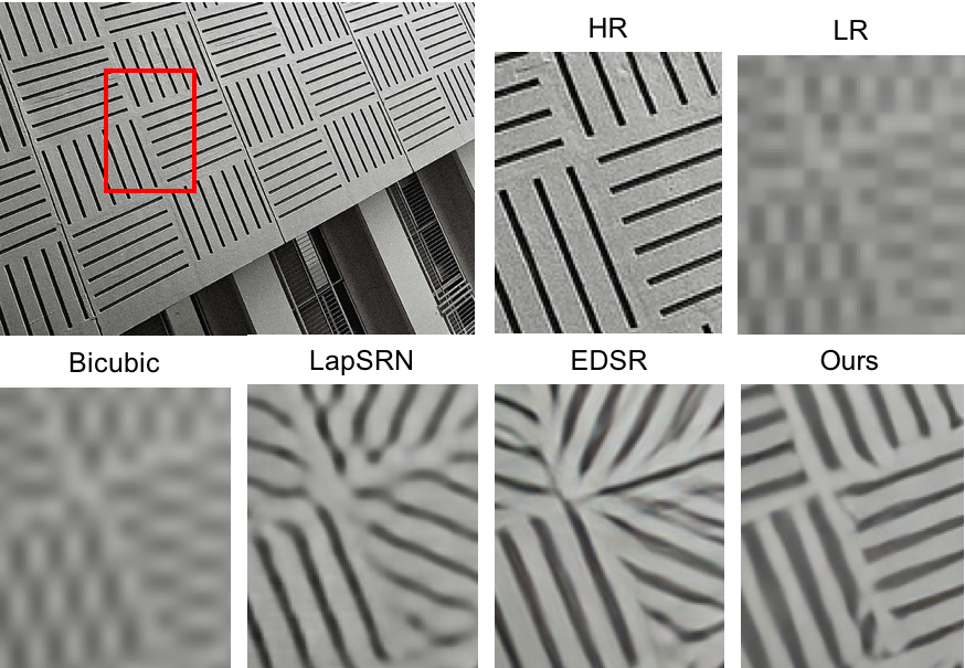
Figure 1: Super-resolution result on $8\times$ enlargement. PSNR: LapSRN [13] (15.25 dB), EDSR [30] (15.33 dB), and Ours [31] (16.63 dB).

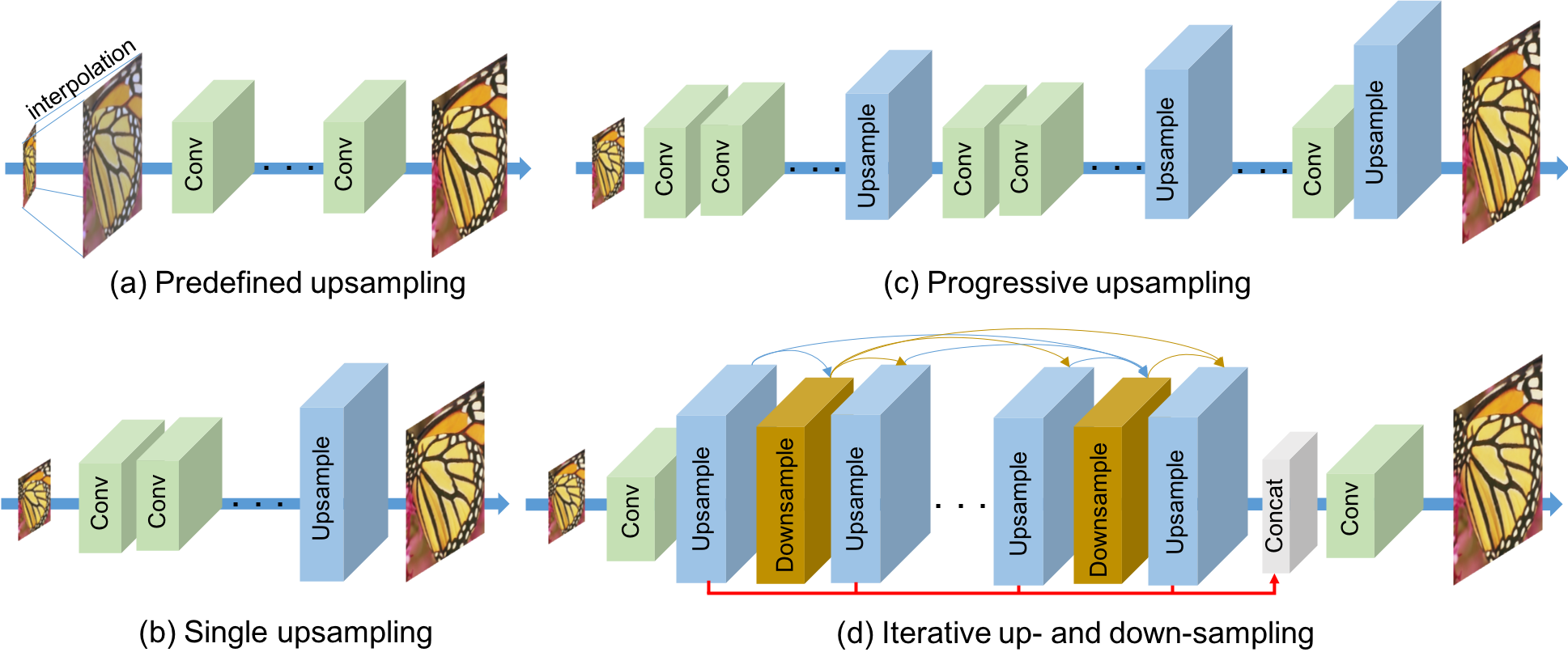
Figure 2: Comparisons of Deep Network SR. (a) Predefined upsampling (e.g., SRCNN [17], VDSR [12], DRRN [14]) commonly uses the conventional interpolation, such as Bicubic, to upscale LR input images before entering the network. (b) Single upsampling (e.g., FSRCNN [18], ESPCN [19]) propagates the LR features, then construct the SR image at the last step. (c) Progressive upsampling uses a Laplacian pyramid network to gradually predict SR images [13]. (d) Iterative up- and down-sampling approach is proposed by our DBPN that exploit the mutually connected up- (blue box) and down-sampling (gold box) units to obtain numerous HR feature maps in different depths.

Inspired by [28], we construct an end-to-end trainable architecture based on the idea of iterative up- and down-sampling layers: Deep Back-Projection Networks (DBPN). Our networks are not only able to remove the ringing and chessboard effect but also successfully perform large scaling factors, as shown in Fig. 1. Furthermore, DBPN has been proven by winning SISR challenges. On NTIRE2018 [32], DBPN is the $1^{st}$ winner on track 8$\times$ Bicubic downscaling. On PIRM2018 [33], DBPN got $1^{st}$ on Region 2, $3^{rd}$ on Region 1, and $5^{th}$ on Region 3.

Our work provides the following contributions:

(1) Iterative up- and down-sampling units. Most of the existing methods extract the feature maps with the same size of LR input image, then these feature maps are finally upsampled to produce SR image directly or progressively. However, DBPN performed iterative up- and down- sampling layers so that it can capture features at each resolution that are helpful in recovering features at other resolution in a single framework. Our networks focus not only on generating variants of the HR features using the up-sampling unit but also on projecting it back to the LR spaces using the down-sampling unit. It is shown in Fig. 2 (d), alternating between up- (blue box) and down-sampling (gold box) units, which represent the mutual relation of LR and HR features. Each set of up- and down-sampling layers achieve data augmentation in the feature space to represent a certain set of features at LR and HR resolution. So, multiple sets of up- and down-sampling layers represent multiple feature maps that are useful for producing the SR image of an input LR image. That is, even if all features extracted by these layers are produced from the single input LR image, these features can be different from each other by training DBPN so that their variety helps to improve its output (i.e., SR image). The detailed explanation can be seen in Section 3.3.

(2) Error feedback. We propose an iterative error-correcting feedback mechanism for SR, which calculates both up- and down-projection errors to guide the reconstruction for obtaining better results. Here, the projection errors are used to refine the initial features in early layers. The detailed explanation can be seen in Section 3.2.

(3) Deep concatenation. Our networks represent different types of LR and HR components produced by each up- and down-sampling unit. This ability enables the networks to reconstruct the HR image using concatenation of the HR feature maps from all of the up-sampling units. Our reconstruction can directly use different types of HR feature maps from different depths without propagating them through the other layers as shown by the red arrows in Fig. 2 (d).

In this work, we make the following extensions to demonstrate a new insight towards more efficient network design substantially compare to our early results [31]. This manuscript focuses on optimized DBPN architecture with advanced design methodologies. The detailed explanation can be seen in Section 4.2. Based on this experiment, we found several technical contributions as follows.

(1) Parameter sharing on projection module. Due to a large amount of parameters, it is hard to train deeper DBPN. Based on our experiments, the deepest setting uses $T=10$. However, using parameter sharing, we can avoid the increasing number of parameters, while widening the receptive field. The effectiveness of parameter sharing was shown in Table VII where DBPN-R64-10 has better performance than D-DBPN while reducing the number of parameters by 10$\times$.

(2) Transition layer on projection step. Inspired by dense connection network [1], we use transition layer to create multiple projection step. The last up- and down-projection units were used as transition layer. The last up-projection was used to produce final HR feature-maps for each iteration, and the last down-projection was used to produce the next input for the next iteration. Table VII shows that DBPN-RES-MR64-3 outperforms previous setting, D-DBPN, by a large margin. DBPN-RES-MR64-3 successfully improves D-DBPN performance by 0.7 dB on Urban100 without increasing the model parameter.

2 Related Work

2.1 Image super-resolution using deep networks

Deep Networks SR can be primarily divided into four types as shown in Fig. 2.

(a) Predefined upsampling commonly uses interpolation as the upsampling operator to produce a middle resolution (MR) image. This scheme was proposed by SRCNN [17] to learn MR-to-HR non-linear mapping with simple convolutional layers as in non deep learning based approaches [23, 21]. Later, the improved networks exploited residual learning [12, 14] and recursive layers [20]. However, this approach has higher computation because the input is the MR image which has the same size as the HR image.

(b) Single upsampling offers a simple way to increase the resolution. This approach was firstly proposed by FSRCNN [18] and ESPCN [19]. These methods have been proven effective to increase the resolution and replace predefined operators. Further improvements include residual network [30], dense connection [34], and channel attention [15] However, they fail to learn complicated mapping of LR-to-HR image, especially on large scaling factors, due to limited feature maps from the LR image. This problem opens the opportunities to propose the mutual relation from LR-to-HR image that can preserve HR components better.

(c) Progressive upsampling was recently proposed in LapSRN [13]. It progressively reconstructs the multiple SR images with different scales in one feed-forward network. For the sake of simplification, we can say that this network is a stacked of single upsampling networks which only relies on limited LR feature maps. Due to this fact, LapSRN is outperformed even by our shallow networks especially for large scaling factors such as $8\times$ in experimental results.

(d) Iterative up- and down-sampling is proposed by our networks [31]. We focus on increasing the sampling rate of HR feature maps in different depths from iterative up- and down-sampling layers, then, distribute the tasks to calculate the reconstruction error on each unit. This scheme enables the networks to preserve the HR components by learning various up- and down-sampling operators while generating deeper features.

2.2 Feedback networks

Rather than learning a non-linear mapping of input-to-target space in one step, the feedback networks compose the prediction process into multiple steps which allow the model to have a self-correcting procedure. Feedback procedure has been implemented in various computing tasks [35, 36, 37, 38, 39, 40, 41].

In the context of human pose estimation, Carreira et al. [35] proposed an iterative error feedback by iteratively estimating and applying a correction to the current estimation. PredNet [41] is an unsupervised recurrent network to predictively code the future frames by recursively feeding the predictions back into the model. For image segmentation, Li et al. [38] learn implicit shape priors and use them to improve the prediction. However, to our knowledge, feedback procedures have not been implemented to SR.

2.3 Adversarial training

Adversarial training, such as with Generative Adversarial Networks (GANs) [42] has been applied to various image reconstruction problems [43, 44, 6, 3, 8]. For the SR task, Johnson et al. [8] introduced perceptual losses based on high-level features extracted from pre-trained networks. Ledig et al. [43] proposed SRGAN which is considered as a single upsampling method. It proposed the natural image manifold that is able to create photo-realistic images by specifically formulating a loss function based on the euclidian distance between feature maps extracted from VGG19 [45]. Our networks can be extended with the adversarial training. The detailed explanation is available in Section 6.

2.4 Back-projection

Back-projection [28] is an efficient iterative procedure to minimize the reconstruction error. Previous studies have proven the effectiveness of back-projection [46, 22, 47, 48]. Originally, back-projection in SR was designed for the case with multiple LR inputs. However, given only one LR input image, the reconstruction procedure can be obtained by upsampling the LR image using multiple upsampling operators and calculate the reconstruction error iteratively [29]. Timofte et al. [48] mentioned that back-projection could improve the quality of the SR images. Zhao et al. [46] proposed a method to refine high-frequency texture details with an iterative projection process. However, the initialization which leads to an optimal solution remains unknown. Most of the previous studies involve constant and unlearned predefined parameters such as blur operator and number of iteration.

3 Deep Back-Projection Networks

Let $I^{h}$ and $I^{l}$ be HR and LR image with $(M^{h}\times N^{h})$ and $(M^{l}\times N^{l})$, respectively, where $M^{l}<M^{h}$ and $N^{l}<N^{h}$. The main building block of our proposed DBPN architecture is the projection unit, which is trained (as part of the end-to-end training of the SR system) to map either an LR feature map to an HR map (up-projection), or an HR map to an LR map (down-projection).

3.1 Iterative back-projection

Back-projection is originally designed with multiple LR inputs [28]. Given only one LR input image, the iterative back-projection [29] can be summarized as follows.

scale up: $$\hat{I}^{h}_{t} =(I^{l}_{t}*p)\uparrow_{s},$$ (1)

scale down: $$\hat{I}^{l}_{t} =(\hat{I}^{h}_{t}*g)\downarrow_{s},$$ (2)

residual: $$e^{l}_{t} =I^{l}_{t}-\hat{I}^{l}_{t},$$ (3)

scale residual up: $$e^{h}_{t} =(e^{l}_{t}*p)\uparrow_{s},$$ (4)

output image: $$\hat{I}^{h}_{t+1} =\hat{I}^{h}_{t}+e^{h}_{t}$$ (5)

where $\hat{I}^{h}_{t+1}$ is the final SR image at the $t$-th iteration, $p$ is a constant back-projection kernel and $g$ is a single blur filter, $\uparrow_{s}$ and $\downarrow_{s}$ are the up- and down-sampling operator, respectively.

The traditional back-projection relies on constant and unlearned predefined parameters such as single sampling filter and blur operator. To extend this algorithm, our proposal preserves the HR components by learned various up- and down-sampling operators and generates deeper features to construct numerous pair of LR-and-HR feature maps. We develop an end-to-end trainable architecture which focuses to guide the SR task using mutually connected up- and down-sampling layers to learn non-linear mutual relation of LR-to-HR components. The mutual relation between LR and HR components is constructed by creating iterative up- and down-projection layers where the up-projection unit generates HR feature maps, then the down-projection unit projects it back to the LR spaces as shown in Fig. 2 (d).

3.2 Projection units

The up-projection unit is defined as follows:

scale up: $$H^{t}_{0} =(L^{t-1}*p_{t})\uparrow_{s},$$ (6)

scale down: $$L^{t}_{0} =(H^{t}_{0}*g_{t})\downarrow_{s},$$ (7)

residual: $$e^{l}_{t} =L^{t}_{0}-L^{t-1},$$ (8)

scale residual up: $$H^{t}_{1} =(e^{l}_{t}*q_{t})\uparrow_{s},$$ (9)

output feature map: $$H^{t} =H^{t}_{0}+H^{t}_{1}$$ (10)

where * is the spatial convolution operator, $\uparrow_{s}$ and $\downarrow_{s}$ are, respectively, the up- and down-sampling operator with scaling factor $s$, and $p_{t},g_{t},q_{t}$ are (de)convolutional layers at stage $t$.

The up-projection unit, illustrated in the upper part of Fig. 3, takes the previously computed LR feature map $L^{t-1}$ as input, and maps it to an (intermediate) HR map $H^{t}_{0}$; then it attempts to map it back to LR map $L^{t}_{0}$ (“back-project”). The residual (difference) $e^{l}_{t}$ between the observed LR map $L^{t-1}$ and the reconstructed $L^{t}_{0}$ is mapped to HR again, producing a new intermediate (residual) map $H^{t}_{1}$; the final output of the unit, the HR map $H^{t}$, is obtained by summing the two intermediate HR maps.

The down-projection unit, illustrated in the lower part of Fig. 3, is defined very similarly, but now its job is to map its input HR map $H^{t}$ to the LR map $L^{t}$.

scale down: $$L^{t}_{0} =(H^{t}*g^{\prime}_{t})\downarrow_{s},$$ (11)

scale up: $$H^{t}_{0} =(L^{t}_{0}*p^{\prime}_{t})\uparrow_{s},$$ (12)

residual: $$e^{h}_{t} =H^{t}_{0}-H^{t},$$ (13)

scale residual down: $$L^{t}_{1} =(e^{h}_{t}*g^{\prime}_{t})\downarrow_{s},$$ (14)

output feature map: $$L^{t} =L^{t}_{0}+L^{t}_{1}$$ (15)

We organize projection units in a series of stages, alternating between $H$ and $L$. These projection units can be understood as a self-correcting procedure which feeds a projection error to the sampling layer and iteratively changes the solution by feeding back the projection error.

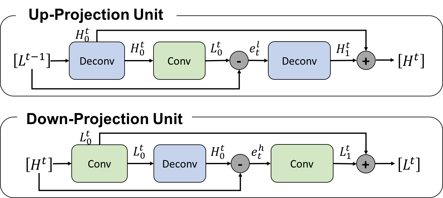
Figure 3: Proposed up- and down-projection units in the DBPN. These units produce residual $e$ between the initial features and the reconstructed features, then fuse it back by summing it to the initial features.

The projection unit uses large sized filters such as $8\times 8$ and $12\times 12$. In the previous approaches, the use of large-sized filters is avoided because it can slow down the convergence speed and might produce sub-optimal results. However, the iterative up- and down-sampling units enable the mutual relation between LR and HR components. These units also take benefit of large receptive fields to perform better performance especially on large scaling factor where the significant amount of pixels is needed.

3.3 Network architecture

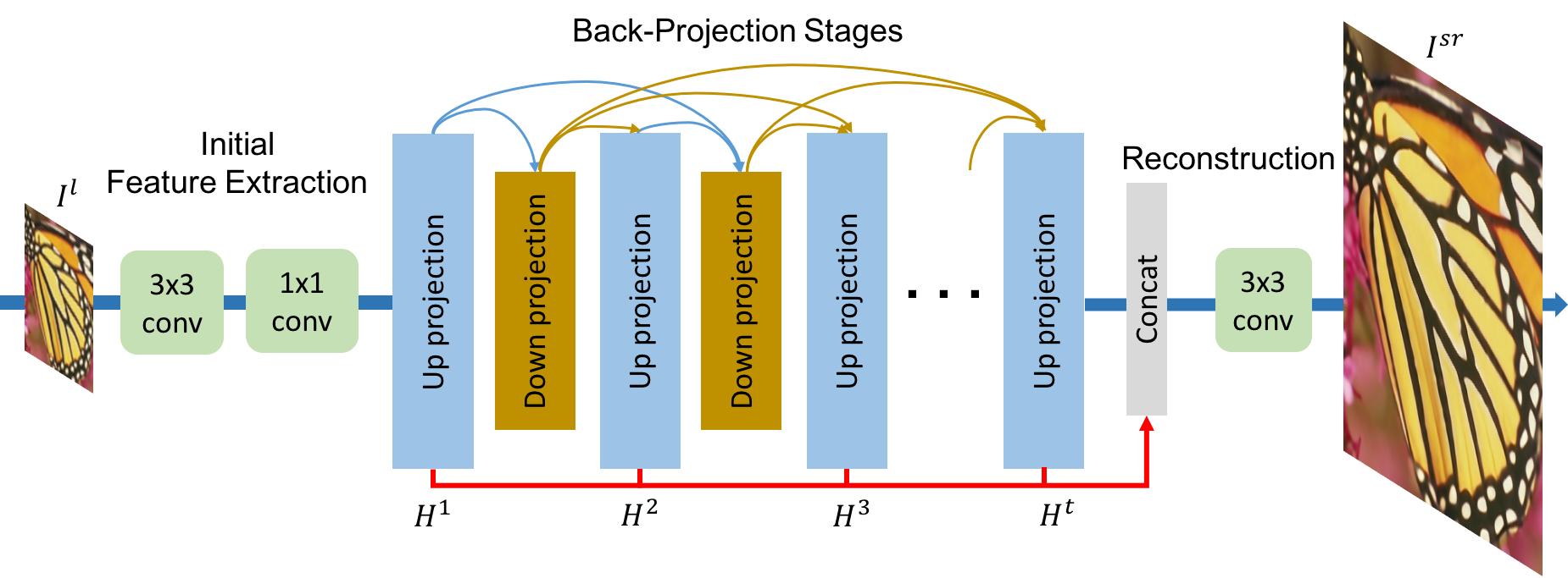
Figure 4: An implementation of DBPN for super-resolution which exploits densely connected projection unit to encourage feature reuse.

The proposed DBPN is illustrated in Fig. 4. It can be divided into three parts: initial feature extraction, projection, and reconstruction, as described below. Here, let conv$(f,n)$ be a convolutional layer, where $f$ is the filter size and $n$ is the number of filters.

1. Initial feature extraction. We construct initial LR feature-maps $L^{0}~{}\in~{}\mathbb{R}^{M^{l}\times N^{l}\times n_{0}}$ from the input using conv$(3,n_{0})$. Then conv$(1,n_{R})$ is used to reduce the dimension from $n_{0}$ to $n_{R}$ before entering projection step where $n_{0}$ is the number of filters used in the initial LR features extraction and $n_{R}$ is the number of filters used in each projection unit.

2. Back-projection stages. Following initial feature extraction is a sequence of projection units, alternating between construction of LR and HR feature maps ($L^{t}~{}\in~{}\mathbb{R}^{M^{l}\times N^{l}\times n_{R}}$ and $H^{t}~{}\in~{}\mathbb{R}^{M^{h}\times N^{h}\times n_{R}}$). Later, it further improves by dense connection where each unit has access to the outputs of all previous units (Section 4.1).

3. Reconstruction. Finally, the target HR image is reconstructed as $I^{sr}=f_{Rec}([H^{1},H^{2},...,H^{t}]),$ where $f_{Rec}$ use conv$(3,3)$ as reconstruction and $[H^{1},H^{2},...,H^{t}]$ refers to the concatenation of the feature-maps produced in each up-projection unit which called as deep concatenation.

Due to the definitions of these building blocks, our network architecture is modular. We can easily define and train networks with different numbers of stages, controlling the depth. For a network with $T$ stages, we have the initial extraction stage (2 layers), and then $T$ up-projection units and $T-1$ down-projection units, each with 3 layers, followed by the reconstruction (one more layer). However, for the dense projection unit, we add conv$(1,n_{R})$ in each projection unit, except the first three units as mentioned in Section 4.1.

4 The Variants of DBPN

In this section, we show how DBPN can be modified to apply the latest deep learning trends.

4.1 Dense projection units

The dense inter-layer connectivity pattern in DenseNets [1] has been shown to alleviate the vanishing-gradient problem, produce improved features, and encourage feature reuse. Inspired by this we propose to improve DBPN, by introducing dense connections in the projection units called, yielding Dense DBPN.

Unlike the original DenseNets, we avoid dropout and batch norm, which are not suitable for SR, because they remove the range flexibility of the features [30]. Instead, we use $1\times 1$ convolution layer as the bottleneck layer for feature pooling and dimensional reduction [49, 11] before entering the projection unit.

In Dense DBPN, the input for each unit is the concatenation of the outputs from all previous units. Let the $L^{\tilde{t}}$ and $H^{\tilde{t}}$ be the input for dense up- and down-projection unit, respectively. They are generated using conv$(1,n_{R})$ which is used to merge all previous outputs from each unit as shown in Fig. 5. This improvement enables us to generate the feature maps effectively, as shown in the experimental results.

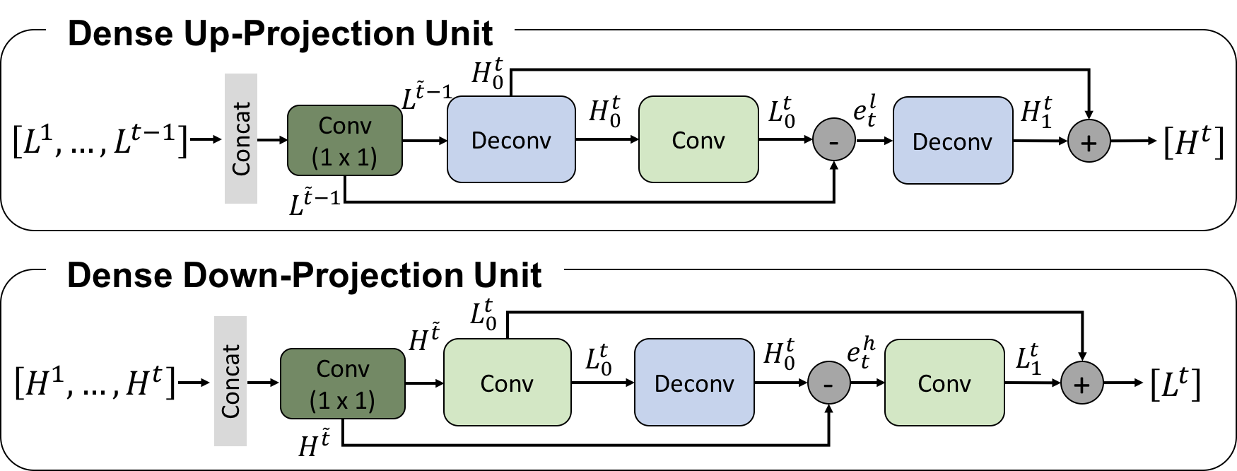
Figure 5: Proposed up- and down-projection unit in the Dense DBPN. The feature maps of all preceding units (i.e., $[L^{1},...,L^{t-1}]$ and $[H^{1},...,H^{t}]$ in up- and down-projections units, respectively) are concatenated and used as inputs, and its own feature maps are used as inputs into all subsequent units.

4.2 Recurrent DBPN

Here, we propose recurrent DBPN which is able to reduce the number of parameters and widen the receptive field without increasing the model capacity. In SISR, DRCN [20] proposed recursive layers without introducing new parameters for additional convolutions in the networks. Then, DRRN [14] improves residual networks by introducing both global and local residual learning using a very deep CNN model (up to 52-layers). DBPN can also be treated as a recurrent network by sharing the projection units across the stages. We divided recurrent DBPN into two variants as mentioned below.

(a) Parameter sharing on projection unit (DBPN-R). This variant uses only one up-projection unit and one down-projection unit which is shared across all stages without dense connection as shown in Fig. 6.

(b) Transition layer on projection step (DBPN-MR). This variant uses multiple up- and down-projection units as shown in Fig. 7. The last up- and down-projection units were used as transition layer. Instead of taking the output from each up-projection unit, DBPN-MR takes the HR features only from the last up-projection unit, then concatenates the HR features from each iteration. Here, the output from the last down-projection unit is the input for the first up-projection layer on the next iteration. Then, the last up-projection unit will receive the output of all previous down-projection units in the corresponding iteration.

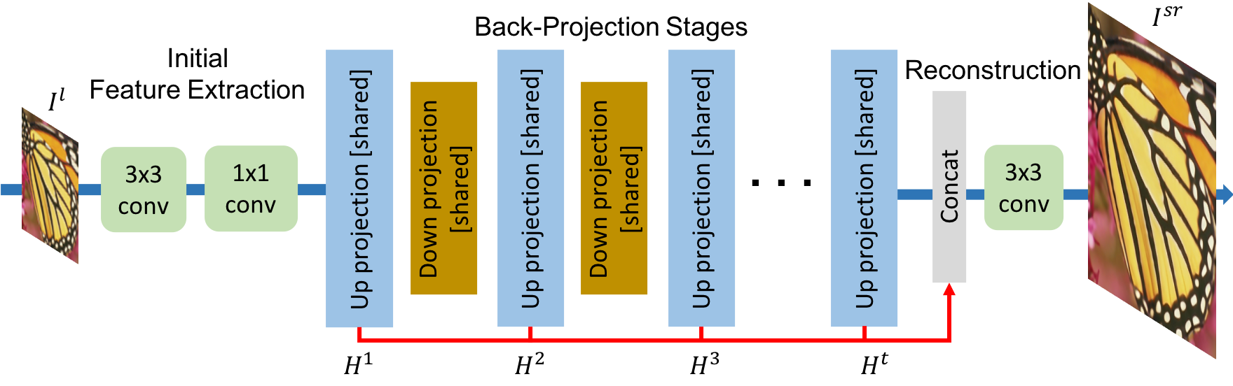
Figure 6: Recurrent DBPN with shared parameter (DBPN-R).

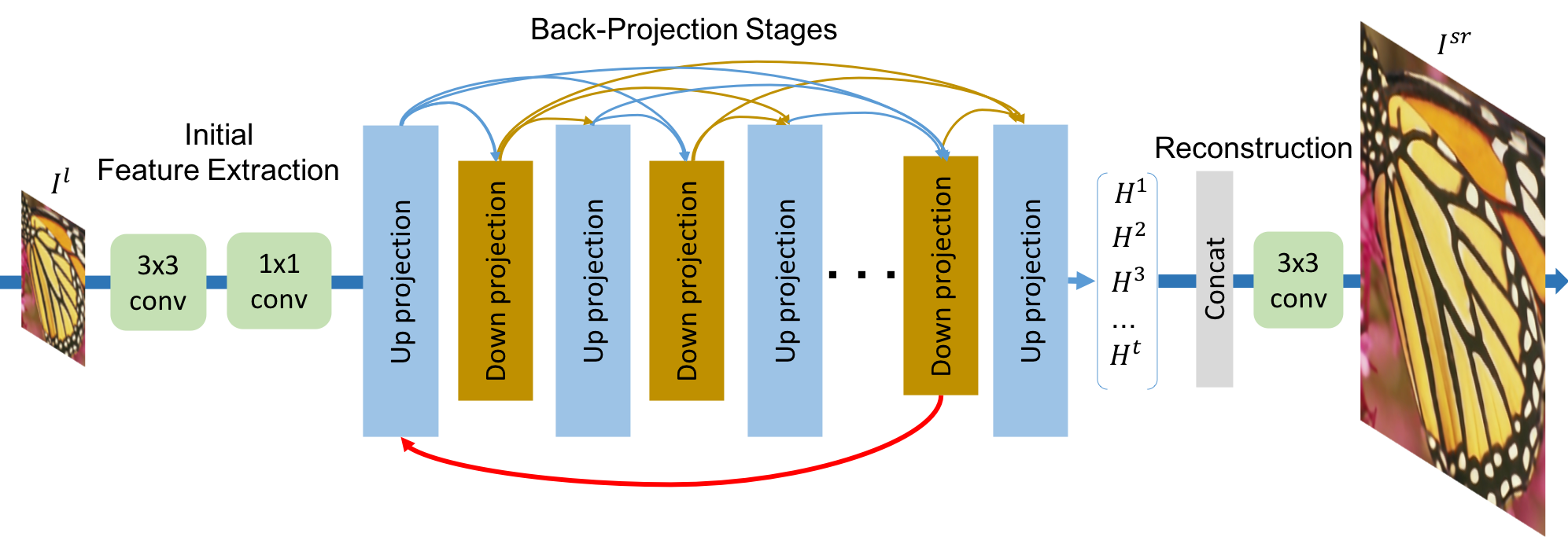
Figure 7: Recurrent DBPN with transition layer (DBPN-MR).

4.3 Residual DBPN

Residual learning helps the network to converge faster and make the network have an easier job to produce only the difference between HR and interpolated LR image. Initially, residual learning has been applied in SR by VDSR [12]. Residual DBPN takes LR image as an input to reduce the computational time. First, LR image is interpolated using Bicubic interpolation; then, at the last stage, the interpolated image is added to the reconstructed image to produce final SR image.

5 Experimental Results

5.1 Implementation and training details

In the proposed networks, the filter size in the projection unit is various with respect to the scaling factor. For $2\times$, we use $6\times 6$ kernel with stride = 2 and pad by 2 pixels. Then, $4\times$ use $8\times 8$ kernel with stride = 4 and pad by 2 pixels. Finally, the $8\times$ use $12\times 12$ kernel with stride = 8 and pad by 2.

We initialize the weights based on [50]. Here, standard deviation (std) is computed by $(\sqrt{2/n_{l}})$ where $n_{l}=f^{2}_{t}n_{t}$, $f_{t}$ is the filter size, and $n_{t}$ is the number of filters. For example, with $f_{t}=3$ and $n_{t}=8$, the std is $0.111$. All convolutional and deconvolutional layers are followed by parametric rectified linear units (PReLUs), except the final reconstruction layer.

We trained all networks using images from DIV2K [51] with augmentation (scaling, rotating, flipping, and random cropping). To produce LR images, we downscale the HR images on particular scaling factors using Bicubic. We use batch size of 16 with size $40\times 40$ for LR image, while HR image size corresponds to the scaling factors. The learning rate is initialized to $1e-4$ for all layers and decrease by a factor of 10 for every $5\times 10^{5}$ iterations for total $10^{6}$ iterations. We used Adam with momentum to $0.9$ and trained with L1 Loss. All experiments were conducted using PyTorch 0.3.1 and Python 3.5 on NVIDIA TITAN X GPUs. The code is available in the internet.

TABLE I: Model architecture of DBPN. ”Feat0” and ”Feat1” refer to first and second convolutional layer in the initial feature extraction stages. Note: ($f,n,st,pd$) where $f$ is filter size, $n$ is number of filters, $st$ is striding, and $pd$ is padding

	Scale	DBPN-SS	DBPN-S	DBPN-M	DBPN-L	D-DBPN-L	D-DBPN	DBPN
Input/Output		Luminance	Luminance	Luminance	Luminance	Luminance	RGB	RGB
Feat0		(3,64,1,1)	(3,128,1,1)	(3,128,1,1)	(3,128,1,1)	(3,128,1,1)	(3,256,1,1)	(3,256,1,1)
Feat1		(1,18,1,0)	(1,32,1,0)	(1,32,1,0)	(1,32,1,0)	(1,32,1,0)	(1,64,1,0)	(1,64,1,0)
Reconstruction		(1,1,1,0)	(1,1,1,0)	(1,1,1,0)	(1,1,1,0)	(1,1,1,0)	(3,3,1,1)	(3,3,1,1)
	$2\times$	(6,18,2,2)	(6,32,2,2)	(6,32,2,2)	(6,32,2,2)	(6,32,2,2)	(6,64,2,2)	(6,64,2,2)
BP stages	$4\times$	(8,18,4,2)	(8,32,4,2)	(8,32,4,2)	(8,32,4,2)	(8,32,4,2)	(8,64,4,2)	(8,64,4,2)
	$8\times$	(12,18,8,2)	(12,32,8,2)	(12,32,8,2)	(12,32,8,2)	(12,32,8,2)	(12,64,8,2)	(12,64,8,2)
	$2\times$	106	337	779	1221	1230	5819	8811
Parameters ($k$)	$4\times$	188	595	1381	2168	2176	10426	15348
	$8\times$	421	1332	3101	4871	4879	23205	34026
Depth		12	12	24	36	40	52	76
No. of stage ($T$)		2	2	4	6	6	7	10
Dense connection		No	No	No	No	Yes	Yes	Yes

5.2 Model analysis

There are six types of DBPN used for model analysis: DBPN-SS, DBPN-S, DBPN-M, DBPN-L, D-DBPN-L, D-DBPN, and DBPN. The detailed architectures of those networks are shown in Table I. Other methods, VDSR [12], DRCN [20], DRRN [14], LapSRN [13], was chosen due to the same nature in number of parameter.

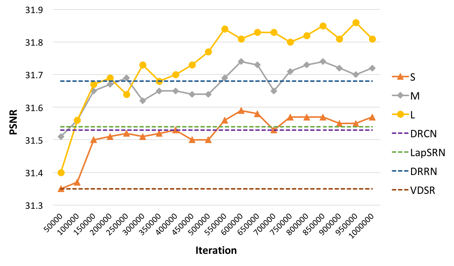
Figure 8: The depth analysis of DBPNs compare to other networks (VDSR [12], DRCN [20], DRRN [14], LapSRN [13]) on Set5 dataset for 4$\times$ enlargement.

Depth analysis. To demonstrate the capability of our projection unit, we construct multiple networks: DBPN-S ($T=2$), DBPN-M ($T=4$), and DBPN-L ($T=6$). In the feature extraction, we use $n_{0}=128$ and $n_{R}=32$. Then, we use $\texttt{conv}(1,1)$ for the reconstruction. The input and output image are luminance only.

The results on $4\times$ enlargement are shown in Fig. 8. From the first $50k$ iteration, our variants are outperformed VDSR. Finally, starting from our shallow network, DBPN-S gives the higher PSNR than VDSR, DRCN, and LapSRN. DBPN-S uses only 12 convolutional layers with smaller number of filters than VDSR, DRCN, and LapSRN. At the best performance, DBPN-S can achieve $31.59$ dB which better $0.24$ dB, $0.06$ dB, $0.05$ dB than VDSR, DRCN, and LapSRN, respectively. DBPN-M shows performance improvement which better than all four existing methods (VDSR, DRCN, LapSRN, and DRRN). At the best performance, DBPN-M can achieve $31.74$ dB which better $0.39$ dB, $0.21$ dB, $0.20$ dB, $0.06$ dB than VDSR, DRCN, LapSRN, and DRRN respectively. In total, DBPN-M uses 24 convolutional layers which has the same depth as LapSRN. Compare to DRRN (up to 52 convolutional layers), DBPN-M undeniable shows the effectiveness of our projection unit. Finally, DBPN-L outperforms all methods with $31.86$ dB which better $0.51$ dB, $0.33$ dB, $0.32$ dB, $0.18$ dB than VDSR, DRCN, LapSRN, and DRRN, respectively.

The results of $8\times$ enlargement are shown in Fig. 9. Our networks outperform the existing networks for $8\times$ enlargement, from the first $50k$ iteration, which clearly show the effectiveness of our proposed networks on large scaling factors. However, we found that there is no significant performance gain from each proposed network especially for DBPN-L and DBPN-M networks where the difference only $0.04$ dB.

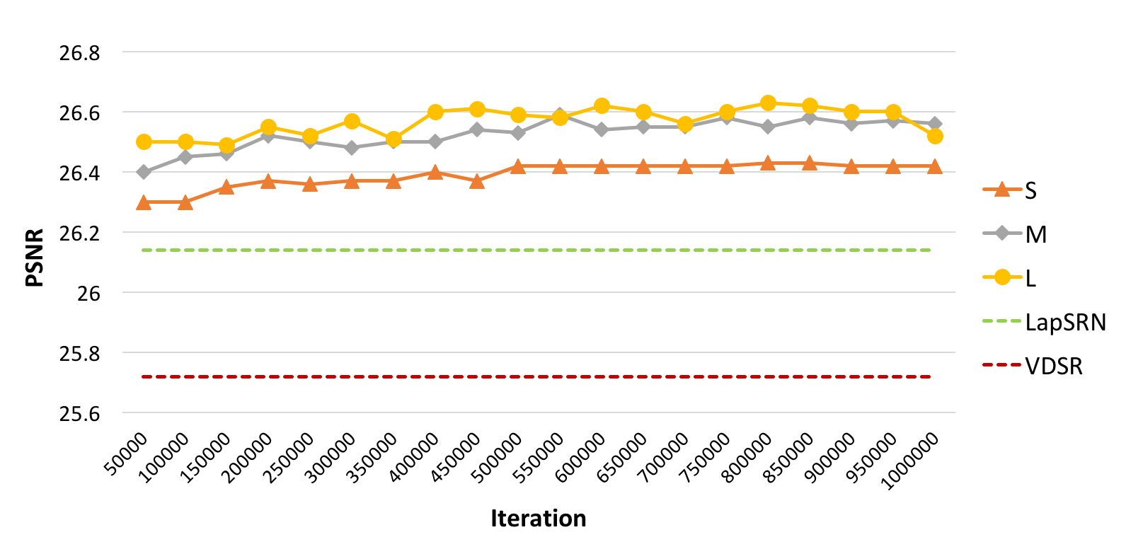
Figure 9: The depth analysis of DBPN on Set5 dataset for 8$\times$ enlargement. DBPN-S ($T=2$), DBPN-M ($T=4$), and DBPN-L ($T=6$)

Number of parameters. We show the tradeoff between performance and number of network parameters from our networks and existing deep network SR in Fig. 11 and 11.

For the sake of low computation for real-time processing, we construct DBPN-SS which is the lighter version of DBPN-S, $(T=2)$. We use $n_{0}=64$ and $n_{R}=18$. However, the results outperform SRCNN, FSRCNN, and VDSR on both $4\times$ and $8\times$ enlargement. Moreover, DBPN-SS performs better than VDSR with $72\%$ and $37\%$ fewer parameters on $4\times$ and $8\times$ enlargement, respectively.

DBPN-S has about $27\%$ fewer parameters and higher PSNR than LapSRN on $4\times$ enlargement. Finally, D-DBPN has about $76\%$ fewer parameters, and approximately the same PSNR, compared to EDSR on $4\times$ enlargement. On the $8\times$ enlargement, D-DBPN has about $47\%$ fewer parameters with better PSNR compare to EDSR. This evidence show that our networks has the best trade-off between performance and number of parameter.

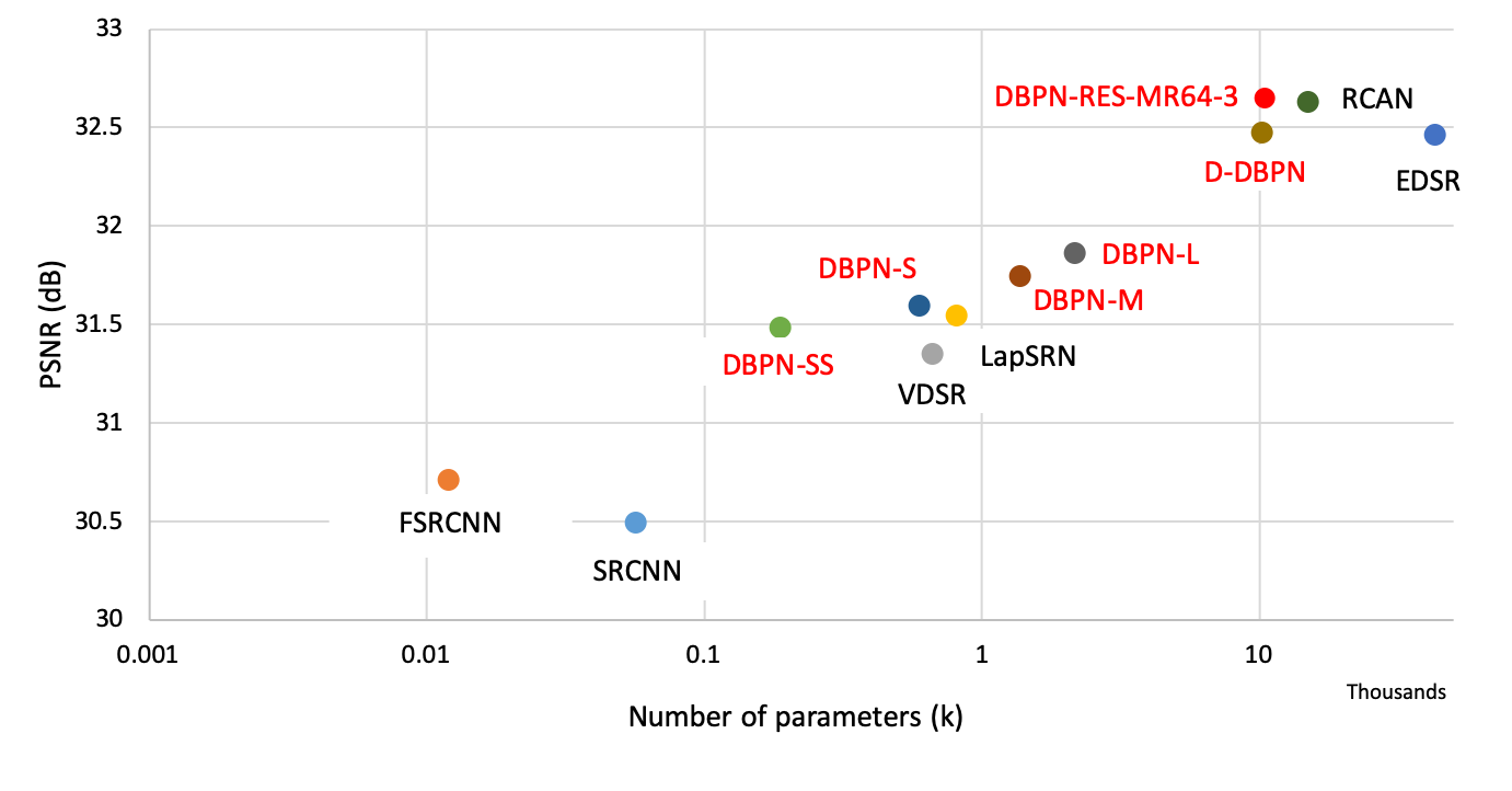
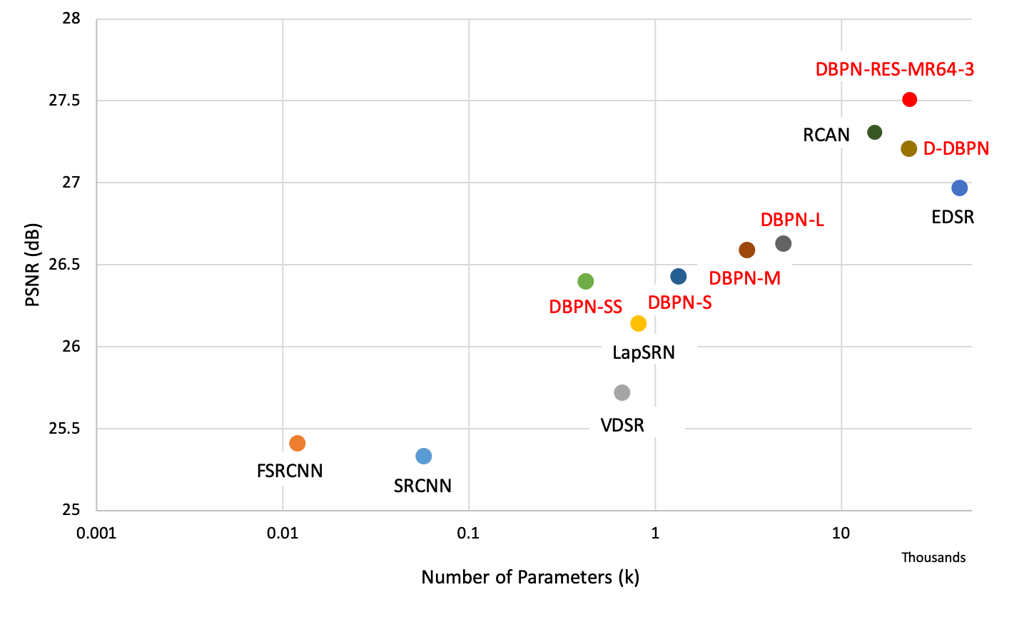
Figure 10: Performance vs number of parameters for $4\times$ enlargement using Set5. The horizontal axis is log-scale.

Figure 11: Performance vs number of parameters for $8\times$ enlargement using Set5. The horizontal axis is log-scale.

Deep concatenation. Each projection unit is used to distribute the reconstruction step by constructing features which represent different details of the HR components. Deep concatenation is also well-related with the number of $T$ (back-projection stage), which shows more detailed features generated from the projection units will also increase the quality of the results. In Fig. 12, it is shown that each stage successfully generates diverse features to reconstruct SR image.

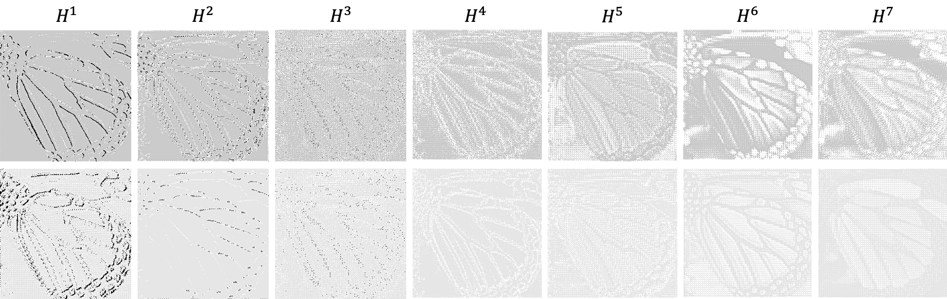
Figure 12: Sample of feature maps from up-projection units in D-DBPN where $t=7$. Each feature has been enhanced using the same grayscale colormap. Zoom in for better visibility.

Error Feedback. As stated before, error feedback (EF) is used to guide the reconstruction in the early layer. Here, we analyze how error feedback can help for better reconstruction. We conduct experiments to see the effectiveness of error feedback procedure. On the scenario without EF, we replace up- and down-projection unit with single up- (deconvolution) and down-sampling (convolution) layer.

We show PSNR of DBPN-S with EF and without EF in Table II. The result with EF has 0.53 dB and 0.26 dB better than without EF on Set5 and Set14, respectively. In Fig. 13, we visually show how error feedback can construct better and sharper HR image especially in the white stripe pattern of the wing.

Moreover, the performance of DBPN-S without EF is interestingly 0.57 dB and 0.35 dB better than previous approaches such as SRCNN [17] and FSRCNN [18], respectively, on Set5. The results show the effectiveness of iterative up- and downsampling layers to demonstrate the LR-to-HR mutual dependency.

TABLE II: Analysis of EF using DBPN-S on $4\times$ enlargement. Red indicates the best performance.

	Set5	Set14
SRCNN [17]	30.49	27.61
FSRCNN [18]	30.71	27.70
Without EF	31.06	27.95
With EF	31.59	28.21

We further analyze the effectiveness of EF comparing the same model size as shown in Table III using D-DBPN model. The better setting is to remove the subtraction (-) and addition (+) operations in the up-/down-projection unit. The results demonstrate the effectiveness of our EF module.

TABLE III: Analysis of EF module on same model size (D-DBPN) on $4\times$ enlargement. Red indicates the best performance.

	D-DBPN-w/ EF	D-DBPN-w/o EF
Set5	32.40/0.897	32.17/0.894
Set14	28.75/0.785	28.56/0/782
BSDS100	27.67/0.738	27.56/0.736
Urban100	26.38/0.793	26.09/0.786
Manga109	30.89/0.913	30.43/0.908

Figure 13: Qualitative comparisons of DBPN-S with EF and without EF on $4\times$ enlargement.

Filter Size We analyze the size of filters which is used in the back-projection stage on D-DBPN model. As stated before, the choice of filter size in the back-projection stage is based on the preliminary results. For the 4$\times$ enlargement, we show that filter 8$\times$8 is 0.08 dB and 0.09 dB better than filter 6$\times$6 and 10$\times$10, respectively, as shown in Table IV.

TABLE IV: Analysis of filter size in the back-projection stages on $4\times$ enlargement from D-DBPN. Red indicates the best performance.

Filter size	Striding	Padding	Set5	Set14
6	4	1	32.39	28.78
8	4	2	32.47	28.82
10	4	3	32.38	28.79

Luminance vs RGB In D-DBPN, we change the input/output from luminance to RGB color channels. There is no significant improvement in the quality of the result as shown in Table V. However, for running time efficiency, constructing all channels simultaneously is faster than a separated process.

TABLE V: Analysis of input/output color channel using DBPN-L. Red indicates the best performance.

	Set5	Set14
RGB	31.88	28.47
Luminance	31.86	28.47

5.3 Comparison of each DBPN variant

Dense connection. We implement D-DBPN-L which is a dense connection of the $L$ network to show how dense connection can improve the network’s performance in all cases as shown in Table VI. On $4\times$ enlargement, the dense network, D-DBPN-L, gains $0.13$ dB and $0.05$ dB higher than DBPN-L on the Set5 and Set14, respectively. On $8\times$, the gaps are even larger. The D-DBPN-L has $0.23$ dB and $0.19$ dB higher that DBPN-L on the Set5 and Set14, respectively.

TABLE VI: Comparison of the DBPN-L and D-DBPN-L on 4$\times$ and 8$\times$ enlargement. Red indicates the best performance.

		Set5		Set14
Algorithm	Scale	PSNR	SSIM	PSNR	SSIM
DBPN-L	4	$31.86$	$0.891$	$28.47$	$0.777$
D-DBPN-L	4	$31.99$	$0.893$	$28.52$	$0.778$
DBPN-L	8	$26.63$	$0.761$	$24.73$	$0.631$
D-DBPN-L	8	$26.86$	$0.773$	$24.92$	$0.638$

Comparison across the variants. We compare six DBPN variants: DBPN-R64-10, DBPN-R128-5, DBPN-MR64-3, DBPN-RES-MR64-3, DBPN-RES, and DBPN. First, DBPN, which was the winner of NTIRE2018 [32] and PIRM2018 [33], uses $n_{0}=256$, $n_{R}=64$, and $t=10$ for the back-projection stages, and dense connection between projection units. In the reconstruction, we use $\texttt{conv}(3,3)$. DBPN-R64-10 uses $n_{R}=64$ with 10 iterations to produce 640 HR features as input of reconstruction layer. DBPN-R128-5, uses $n_{R}=128$ with 5 iterations, produces 640 HR features. DBPN-MR64-3 has the same architecture with D-DBPN but the projection units are treated as recurrent network. DBPN-RES-MR64-3 is DBPN-MR64-3 with residual learning. Last, DBPN-RES is DBPN with residual learning. All variants are trained with the same training setup.

The results are shown in Table VII. It shows that all variants successfully have better performance than D-DBPN [31]. DBPN-R64-10 has the least parameter compare to other variants, which is suitable for mobile/real-time application. It can reduce $10\times$ number of parameter compare to DBPN and maintain to get good performance. We can see that increasing $n_{R}$ can improve the performance of DBPN-R which is shown by DBPN-R128-5 compare to DBPN-R64-10. However, better results is obtained by DBPN-MR64-3, especially on Urban100 and Manga109 test set compare to other variants. It is also proven that residual learning can slightly improve the performance of DBPN. Therefore, it is natural that we performed the combination of multiple stages recurrent and residual learning called DBPN-RES-MR64-3 which performs the best results and has lower parameter than DBPN.

TABLE VII: Quantitative evaluation of DBPN’s variants on 4$\times$. Red indicates the best performance.

		Set5		Set14		BSDS100		Urban100		Manga109
Method	# Parameters ($k$)	PSNR	SSIM	PSNR	SSIM	PSNR	SSIM	PSNR	SSIM	PSNR	SSIM
D-DBPN [31]	10426	$32.40$	$0.897$	$28.75$	$0.785$	$27.67$	$0.738$	$26.38$	$0.793$	$30.89$	$0.913$
DBPN	15348	$32.55$	$0.898$	$28.91$	$0.789$	$27.77$	$0.742$	$26.82$	$0.807$	$31.46$	$0.918$
DBPN-R64-10	1614	$32.38$	$0.896$	$28.83$	$0.787$	$27.73$	$0.740$	$26.51$	$0.798$	$31.12$	$0.915$
DBPN-R128-5	6349	$32.41$	$0.897$	$28.83$	$0.787$	$27.72$	$0.740$	$26.58$	$0.799$	$31.15$	$0.915$
DBPN-MR64-3	10419	$32.57$	$0.898$	$28.92$	$0.790$	$27.79$	$0.743$	$26.92$	$0.810$	$31.51$	$0.919$
DBPN-RES	15348	$32.54$	$0.897$	$28.92$	$0.789$	$27.79$	$0.742$	$26.89$	$0.808$	$31.49$	$0.918$
DBPN-RES-MR64-3	10419	$32.65$	$0.899$	$29.03$	$0.791$	$27.82$	$0.744$	$27.08$	$0.814$	$31.74$	$0.921$

5.4 Comparison with the-state-of-the-arts on SR

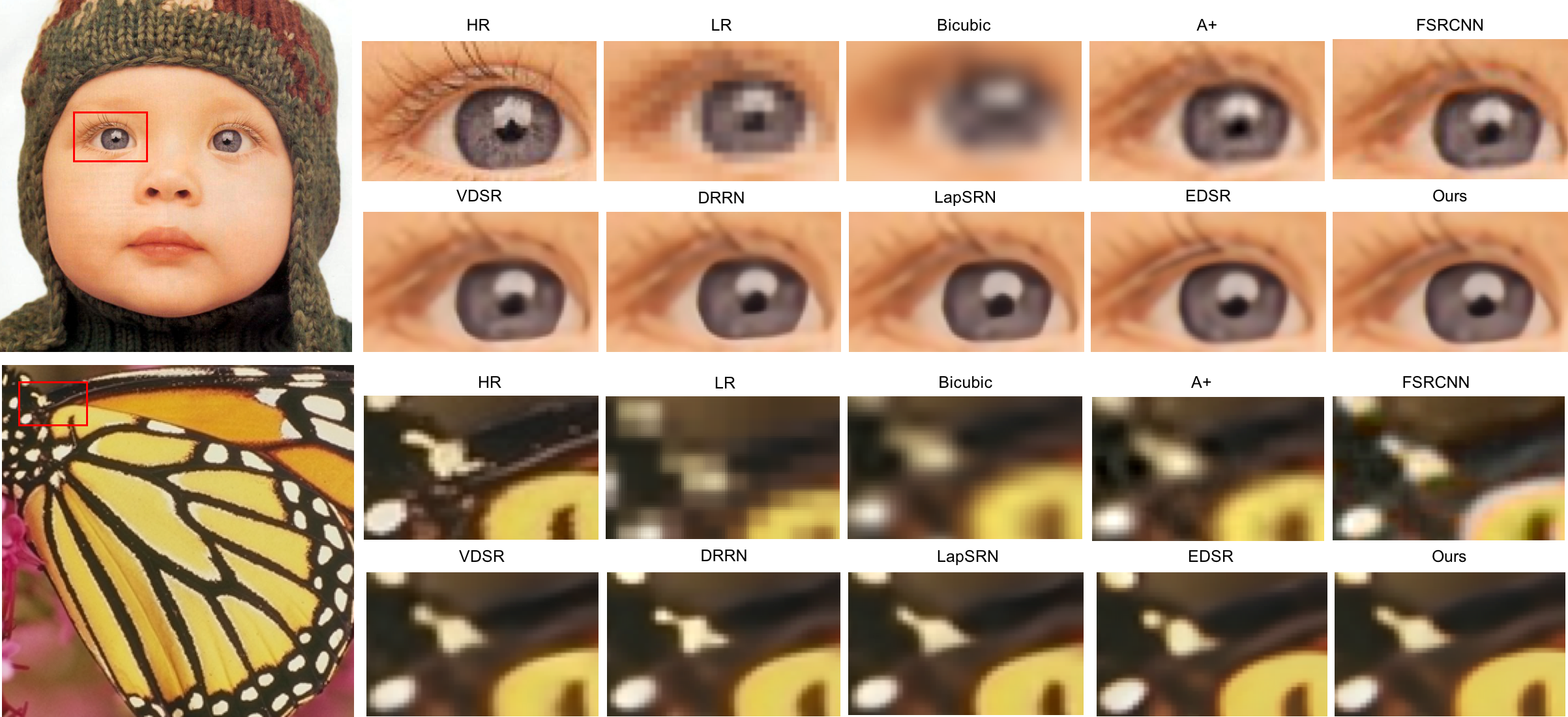
Figure 14: Qualitative comparison of our models with other works on $4\times$ super-resolution.

To confirm the ability of the proposed network, we performed several experiments and analysis. We compare our network with 14 state-of-the-art SR algorithms: A+ [23], SRCNN [17], FSRCNN [18], VDSR [12], DRCN [20], DRRN [14], LapSRN [13], MS-LapSRN [52], MSRN [53], D-DBPN [31], EDSR [30], RDN [34], RCAN [15], and SAN [54]. We carry out extensive experiments using 5 datasets: Set5 [55], Set14 [56], BSDS100 [57], Urban100 [58] and Manga109 [59]. Each dataset has different characteristics. Set5, Set14 and BSDS100 consist of natural scenes; Urban100 contains urban scenes with details in different frequency bands; and Manga109 is a dataset of Japanese manga.

Our final network, DBPN-RES-MR64-3, combines dense connection, recurrent network and residual learning to boost the performance of DBPN. It uses $n_{0}=256$, $n_{R}=64$, and $t=7$ with 3 iteration. In the reconstruction, we use $\texttt{conv}(3,3)$. RGB color channels are used for input and output image. It takes around 14 days to train.

PSNR and structural similarity (SSIM) [60] were used to quantitatively evaluate the proposed method. Note that higher PSNR and SSIM values indicate better quality. As used by existing networks, all measurements used only the luminance channel (Y). For SR by factor $s$, we crop $s$ pixels near image boundary before evaluation as in [30, 18]. Some of the existing networks such as SRCNN, FSRCNN, VDSR, and EDSR did not perform $8\times$ enlargement. To this end, we retrained the existing networks by using author’s code with the recommended parameters.

Figure 14 shows that EDSR tends to generate stronger edge than the ground truth and lead to misleading information in several cases. The result of EDSR shows the eyelashes were interpreted as a stripe pattern. Our result generates softer patterns which is subjectively closer to the ground truth. On the butterfly image, EDSR separates the white pattern and tends to construct regular pattern such ac circle and stripe, while D-DBPN constructs the same pattern as the ground truth.

We show the quantitative results in the Table VIII. Our network outperforms the existing methods by a large margin in all scales except RCAN and SAN on $2\times$. For $4\times$, EDSR has $0.26$ dB higher than D-DBPN but outperformed by DBPN-RES-MR64-3 with $0.44$ dB margin on Urban100. Recent state-of-the-art, SAN [54] and RCAN [15], performs better results than our network on $2\times$. However, on $4\times$, our network has $0.26$ dB higher than RCAN on Urban100. The biggest gap is shown on Manga109, our network has $0.52$ dB higher than RCAN.

Our network shows its effectiveness on $8\times$ enlargement which outperforms all of the existing methods by a large margin. Interesting results are shown on Manga109 dataset where D-DBPN obtains $25.50$ dB which is $0.61$ dB better than EDSR. While on the Urban100 dataset, D-DBPN achieves 23.25 which is only $0.13$ dB better than EDSR. Our final network, DBPN-RES-MR64-3, outperforms all previous networks. DBPN-RES-MR64-3 is roughly $0.2$ dB better than RCAN [15] across multiple dataset. The biggest gap is on Manga109 where DBPN-RES-MR64-3 is $0.47$ dB better than RCAN [15]. The overall results show that our networks perform better on fine-structures images especially manga characters, even though we do not use any animation images in the training.

The results of $8\times$ enlargement are visually shown in Fig. 15. Qualitatively, our network is able to preserve the HR components better than other networks. For image “img$\_040$.png”, all of previous methods fail to recover the correct direction of the image textures, while ours produce more faithful results to the ground truth. For image “Hamlet$\_2$.png”, other methods suffer from heavy blurring artifacts and fail to recover the details. While, our network successfully recovers the fined detail and produce the closest result to the ground truth. It shows that our networks can successfully extract not only features but also create contextual information from the LR input to generate HR components in the case of large scaling factors, such as $8\times$ enlargement.

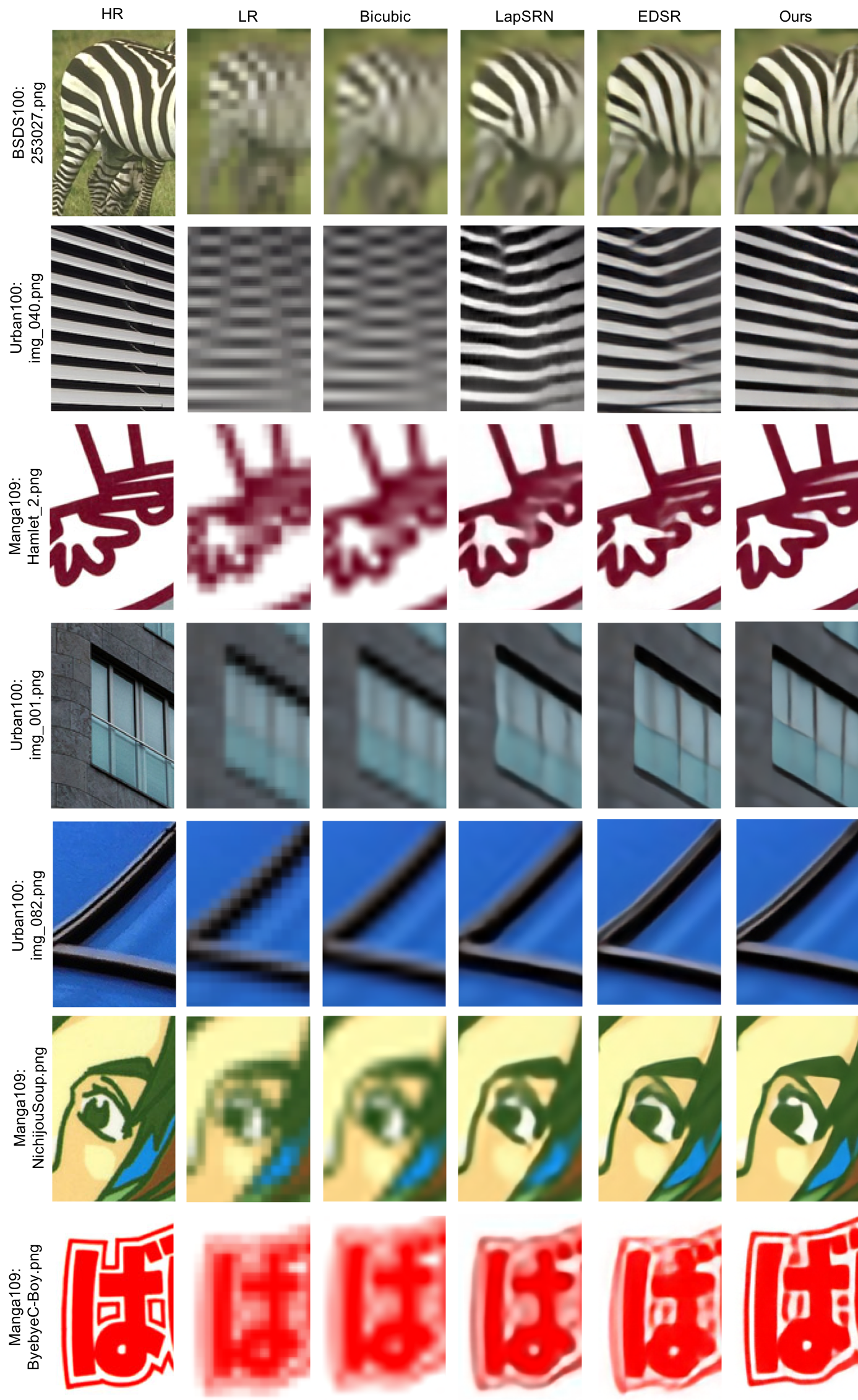
Figure 15: Qualitative comparison of our models with other works on $8\times$ super-resolution.

TABLE VIII: Quantitative evaluation of state-of-the-art SR algorithms: average PSNR/SSIM for scale factors 2$\times$, 4$\times$, and 8$\times$. Red indicates the best and blue indicates the second best performance.

			Set5		Set14		BSDS100		Urban100		Manga109
Method	Scale	# Parameters ($M$)	PSNR	SSIM	PSNR	SSIM	PSNR	SSIM	PSNR	SSIM	PSNR	SSIM
Bicubic	2	-	$33.65$	$0.930$	$30.34$	$0.870$	$29.56$	$0.844$	$26.88$	$0.841$	$30.84$	$0.935$
A+ [23]	2	-	$36.54$	$0.954$	$32.40$	$0.906$	$31.22$	$0.887$	$29.23$	$0.894$	$35.33$	$0.967$
SRCNN [17]	2	0.05M	$36.65$	$0.954$	$32.29$	$0.903$	$31.36$	$0.888$	$29.52$	$0.895$	$35.72$	$0.968$
FSRCNN [18]	2	0.01M	$36.99$	$0.955$	$32.73$	$0.909$	$31.51$	$0.891$	$29.87$	$0.901$	$36.62$	$0.971$
VDSR [12]	2	0.66M	$37.53$	$0.958$	$32.97$	$0.913$	$31.90$	$0.896$	$30.77$	$0.914$	$37.16$	$0.974$
DRCN [20]	2	1.77M	$37.63$	$0.959$	$32.98$	$0.913$	$31.85$	$0.894$	$30.76$	$0.913$	$37.57$	$0.973$
DRRN [14]	2	0.30M	$37.74$	$0.959$	$33.23$	$0.913$	$32.05$	$0.897$	$31.23$	$0.919$	$37.92$	$0.976$
LapSRN [13]	2	0.81M	$37.52$	$0.959$	$33.08$	$0.913$	$31.80$	$0.895$	$30.41$	$0.910$	$37.27$	$0.974$
MS-LapSRN [52]	2	0.22M	$37.78$	$0.960$	$33.28$	$0.915$	$32.05$	$0.898$	$31.15$	$0.919$	$37.78$	$0.976$
MSRN [53]	2	6.3M	$38.08$	$0.960$	$33.74$	$0.917$	$32.23$	$0.901$	$32.22$	$0.932$	$38.82$	$0.987$
D-DBPN [31]	2	5.82M	$38.05$	$0.960$	$33.79$	$0.919$	$32.25$	$0.900$	$32.51$	$0.932$	$38.81$	$0.976$
RDN [34]	2	22.3M	$38.24$	$0.961$	$34.01$	$0.921$	$32.34$	$0.902$	$32.89$	$0.935$	$39.18$	$0.978$
RCAN [15]	2	16M	$38.27$	$0.961$	$34.12$	$0.921$	$32.41$	$0.903$	$33.34$	$0.938$	$39.44$	$0.979$
SAN [54]	2	15.7M	$38.31$	$0.962$	$34.07$	$0.921$	$32.42$	$0.903$	$33.10$	$0.937$	$39.32$	$0.979$
DBPN-RES-MR64-3	2	5.82M	$38.08$	$0.960$	$34.09$	$0.921$	$32.31$	$0.901$	$32.92$	$0.935$	$39.28$	$0.977$
Bicubic	4	-	$28.42$	$0.810$	$26.10$	$0.704$	$25.96$	$0.669$	$23.15$	$0.659$	$24.92$	$0.789$
A+ [23]	4	-	$30.30$	$0.859$	$27.43$	$0.752$	$26.82$	$0.710$	$24.34$	$0.720$	$27.02$	$0.850$
SRCNN [17]	4	0.05M	$30.49$	$0.862$	$27.61$	$0.754$	$26.91$	$0.712$	$24.53$	$0.724$	$27.66$	$0.858$
FSRCNN [18]	4	0.01M	$30.71$	$0.865$	$27.70$	$0.756$	$26.97$	$0.714$	$24.61$	$0.727$	$27.89$	$0.859$
VDSR [12]	4	0.66M	$31.35$	$0.882$	$28.03$	$0.770$	$27.29$	$0.726$	$25.18$	$0.753$	$28.82$	$0.886$
DRCN [20]	4	1.77M	$31.53$	$0.884$	$28.04$	$0.770$	$27.24$	$0.724$	$25.14$	$0.752$	$28.97$	$0.886$
DRRN [14]	4	0.30M	$31.68$	$0.888$	$28.21$	$0.772$	$27.38$	$0.728$	$25.44$	$0.764$	$29.46$	$0.896$
LapSRN [13]	4	0.81M	$31.54$	$0.885$	$28.19$	$0.772$	$27.32$	$0.728$	$25.21$	$0.756$	$29.09$	$0.890$
MS-LapSRN [52]	4	0.22M	$31.74$	$0.889$	$28.26$	$0.774$	$27.43$	$0.731$	$25.51$	$0.768$	$29.54$	$0.897$
MSRN [53]	4	6.3M	$32.07$	$0.890$	$28.60$	$0.775$	$27.52$	$0.727$	$26.04$	$0.789$	$30.17$	$0.903$
D-DBPN [31]	4	10.2M	$32.40$	$0.897$	$28.75$	$0.785$	$27.67$	$0.738$	$26.38$	$0.793$	$30.89$	$0.913$
EDSR [30]	4	43.2M	$32.46$	$0.897$	$28.80$	$0.788$	$27.71$	$0.742$	$26.64$	$0.803$	$31.02$	$0.915$
RDN [34]	4	22.3M	$32.47$	$0.899$	$28.81$	$0.787$	$27.72$	$0.742$	$26.61$	$0.803$	$31.00$	$0.915$
RCAN [15]	4	16M	$32.63$	$0.900$	$28.87$	$0.789$	$27.77$	$0.744$	$26.82$	$0.809$	$31.22$	$0.917$
SAN [54]	4	15.7M	$32.64$	$0.900$	$28.92$	$0.789$	$27.78$	$0.743$	$26.79$	$0.807$	$31.18$	$0.917$
DBPN-RES-MR64-3	4	10.2M	$32.65$	$0.899$	$29.03$	$0.791$	$27.82$	$0.744$	$27.08$	$0.814$	$31.74$	$0.921$
Bicubic	8	-	$24.39$	$0.657$	$23.19$	$0.568$	$23.67$	$0.547$	$20.74$	$0.516$	$21.47$	$0.647$
A+ [23]	8	-	$25.52$	$0.692$	$23.98$	$0.597$	$24.20$	$0.568$	$21.37$	$0.545$	$22.39$	$0.680$
SRCNN [17]	8	0.05M	$25.33$	$0.689$	$23.85$	$0.593$	$24.13$	$0.565$	$21.29$	$0.543$	$22.37$	$0.682$
FSRCNN [18]	8	0.01M	$25.41$	$0.682$	$23.93$	$0.592$	$24.21$	$0.567$	$21.32$	$0.537$	$22.39$	$0.672$
VDSR [12]	8	0.66M	$25.72$	$0.711$	$24.21$	$0.609$	$24.37$	$0.576$	$21.54$	$0.560$	$22.83$	$0.707$
LapSRN [13]	8	0.81M	$26.14$	$0.738$	$24.44$	$0.623$	$24.54$	$0.586$	$21.81$	$0.582$	$23.39$	$0.735$
MS-LapSRN [52]	8	0.22M	$26.34$	$0.753$	$24.57$	$0.629$	$24.65$	$0.592$	$22.06$	$0.598$	$23.90$	$0.759$
MSRN [53]	8	6.3M	$26.59$	$0.725$	$24.88$	$0.5961$	$24.70$	$0.541$	$22.37$	$0.598$	$24.28$	$0.752$
D-DBPN [31]	8	23.1M	$27.25$	$0.785$	$25.14$	$0.649$	$24.91$	$0.602$	$22.72$	$0.630$	$25.14$	$0.798$
EDSR [30]	8	43.2M	$26.97$	$0.775$	$24.94$	$0.640$	$24.80$	$0.596$	$22.47$	$0.620$	$24.58$	$0.778$
RCAN [15]	8	16M	$27.31$	$0.787$	$25.23$	$0.651$	$24.98$	$0.606$	$23.00$	$0.645$	$25.24$	$0.803$
SAN [54]	8	15.7M	$27.22$	$0.783$	$25.14$	$0.648$	$24.88$	$0.601$	$22.70$	$0.631$	$24.85$	$0.791$
DBPN-RES-MR64-3	8	23.1M	$27.51$	$0.793$	$25.41$	$0.657$	$25.05$	$0.607$	$23.20$	$0.652$	$25.71$	$0.813$

5.5 Runtime Evaluation

We present the runtime comparisons between our networks and three existing methods: VDSR [12], DRRN [14], and EDSR [30]. The comparison must be done in fair settings. The runtime is calculated using python function timeit which encapsulating only forward function. For EDSR, we use original author code based on Torch and use timer function to obtain the runtime.

We evaluate each network using NVIDIA TITAN X GPU (12G Memory). The input image size is 64$\times$ 64, then upscaled into 128$\times$ 128 (2$\times$), 256$\times$ 256 (4$\times$), and 512$\times$ 512 (8$\times$). The results are the average of 10 times trials.

Table IX shows the runtime comparisons on 2$\times$, 4$\times$, and 8$\times$ enlargement. It shows that DBPN-SS and DBPN-S obtain the best and second best performance on 2$\times$, 4$\times$, and 8$\times$ enlargement. Compare to EDSR, D-DBPN shows its effectiveness by having faster runtime with comparable quality on 2$\times$ and 4$\times$ enlargement. On 8$\times$ enlargement, the gap is bigger. It shows that D-DBPN has better results with lower runtime than EDSR.

Noted that input for VDSR and DRRN is only luminance channel and need preprocessing to create middle-resolution image. So that, the runtime should be added by additional computation of interpolation computation on preprocessing.

TABLE IX: Runtime evaluation with input size 64$\times$64. Red indicates the best and blue indicates the second best performance, * indicates the calculation using function timer in Torch, and N.A. indicates that the algorithm runs out of GPU memory.

	$2\times$	$4\times$	$8\times$
	(128$\times$128)	(256$\times$256)	(512$\times$512)
VDSR [12]	0.022	0.032	0.068
DRRN [14]	0.254	0.328	N.A.
*EDSR [30]	0.857	1.245	1.147
DBPN-SS	0.012	0.016	0.026
DBPN-S	0.013	0.020	0.038
DBPN-M	0.023	0.045	0.081
DBPN-L	0.035	0.069	0.126
D-DBPN	0.153	0.193	0.318
DBPN-RES-MR64-3	0.171	0.227	0.339

6 Perceptually optimized DBPN

We also can extend DBPN to produce HR outputs that appear to be better under human perception. Despite many attempts, it remains unclear how to accurately model perceptual quality. Instead, we incorporate the perceptual quality into the generator by using adversarial loss, as introduced elsewhere [43, 44, 61]. In the adversarial settings, there are two building blocks: a generator ($G$) and a discriminator ($D$). In the context of SR, the generator $G$ produces HR images (from LR inputs). The discriminator $D$ works to differentiate between real HR images and generated HR images (the product of SR network $G$). In our experiments, the generator is a DBPN network, and the discriminator is a network with five hidden layers with batch norm, followed by the last, fully connected layer.

TABLE X: PIRM2018 Challenge results [33]. The top 9 submissions in each region. For submissions with a marginal PI difference (up to 0.01), the one with the lower RMSE is ranked higher. Submission with marginal differences in both the PI and RMSE are ranked together (marked by $*$).

Region 1					Region 2					Region 3
#	Team	PI	RMSE		#	Team	PI	RMSE		#	Team	PI	RMSE
$1$	IPCV [62]	2.709	11.48		$1$	TTI (Ours)	2.199	12.40		$1$	SuperSR [63]	1.978	15.30
$2$	MCML [64]	2.750	11.44		$2*$	IPCV [62]	2.275	12.47		$2$	BOE [65]	2.019	14.24
$3*$	SuperSR [63]	2.933	11.50		$2*$	MCML [66]	2.279	12.41		$3$	IPCV [62]	2.013	15.26
$3*$	TTI (Ours)	2.938	11.46		$4$	SuperSR [63]	2.424	12.50		$4$	AIM [67]	2.013	15.60
$5$	AIM [67]	3.321	11.37		$5$	BOE [65]	2.484	12.50		$5$	TTI (Ours)	2.040	13.17
$6$	DSP-whu	3.728	11.45		$6$	AIM [67]	2.600	12.42		$6$	Haiyun [68]	2.077	15.95
$7*$	BOE [65]	3.817	11.50		$7$	REC-SR [69]	2.635	12.37		$7$	gayNet	2.104	15.88
$7*$	REC-SR [69]	3.831	11.46		$8$	DSP-whu	2.660	12.24		$8$	DSP-whu	2.114	15.93
$9$	Haiyun [68]	4.440	11.19		$9$	XYN	2.946	12.23		$9$	MCML	2.136	13.44

The generator loss in this experiment is composed of four loss terms, following [44]: MSE, VGG, Style, and Adversarial loss.

$$L_{G}=w_{1}*L_{mse}+w_{2}*L_{vgg}+w_{3}*L_{adv}+w_{4}*L_{style}$$ (16)

• MSE loss is pixel-wise loss which calculated in the image space $L_{mse}=||I^{h}-I^{sr}||^{2}_{2}$.

• VGG loss is calculated in the feature space using pretrained VGG19 network [45] on multiple layers. This loss was originally proposed by [8, 70]. Both $I^{h}$ and $I^{sr}$ are first mapped into a feature space by differentiable functions $f_{i}$ from VGG multiple max-pool layers ${(i={2,3,4,5})}$ then sum up each layer distances. $L_{vgg}=\sum\limits_{i={2}}^{5}||f_{i}(I^{h})-f_{i}(I^{sr})||^{2}_{2}$.

• Adversarial loss. $L_{adv}=-\texttt{log}(D(G(I^{l})))$, where $D(x)$ is the probability assigned by $D$ to $x$ being a real HR image.

• Style loss is used to generate high quality textures. This loss was originally proposed by [71] which is later modified by [44]. Style loss uses the same differentiable function $f$ as in VGG loss. $L_{style}=\sum\limits_{i={2}}^{5}||\theta(f_{i}(I^{h}))-\theta(f_{i}(I^{sr}))||^{2}_{2}$ where Gram matrix $\theta(F)=FF^{T}\in\mathbb{R}^{n\times n}$.

The training objective for $D$ is

$$L_{D}=-\texttt{log}(D(I^{h}))-\texttt{log}(1-D(G(I^{l}))).$$

As is common in training adversarial networks, we alternate between stages of training $G$ and training $D$. We use pre-trained DBPN model which optimized by MSE loss only, then fine-tuned with the perceptual loss. We use batch size of 4 with size $60\times 60$ for LR image, while HR image size is $240\times 240$. The learning rate is initialized to $1e-4$ for all layers for $2\times 10^{5}$ iteration using Adam with momentum to $0.9$.

This method was included in the challenge associated with PIRM2018 [33], in conjunction with ECCV 2018. In the challenge, evaluation was conducted in three disjoint regimes defined by thresholds on the RMSE; the intuition behind this is the natural tradeoff between RMSE and perceptual quality of the reconstruction. The latter is measured by combining the quality measures of Ma [72] and NIQE [73] as below,

$$\texttt{Perceptual index}=1/2((10-Ma)+NIQE).$$ (17)

The three regimes correspond to Region 1: RMSE $\leq 11.5$ , Region 2: $11.5<$ RMSE $\leq 12.5$, and Region 3: $12.5<$ RMSE $\leq 16$. We select optimal parameter settings for each regime. This process yields

• Region 1 ($w_{1}:0.5,w_{2}:0.05,w_{3}:0.001,w_{4}:1$)

• Region 2 ($w_{1}:0.1,w_{2}:0.2,w_{3}:0.001,w_{4}:1$)

• Region 3 ($w_{1}:0.03,w_{2}:0.2,w_{3}:0.001,w_{4}:10$)

Our method achieved $1^{st}$ place on Region 2, $3^{rd}$ place on Region 1, and $5^{th}$ place on Region 3 [33] as shown in Table X. In Region 3, it shows very competitive results where we got $5^{th}$, however, it is noted that our method has the lowest RMSE among other top 5 performers which means the image has less distortion or hallucination w.r.t the original image.

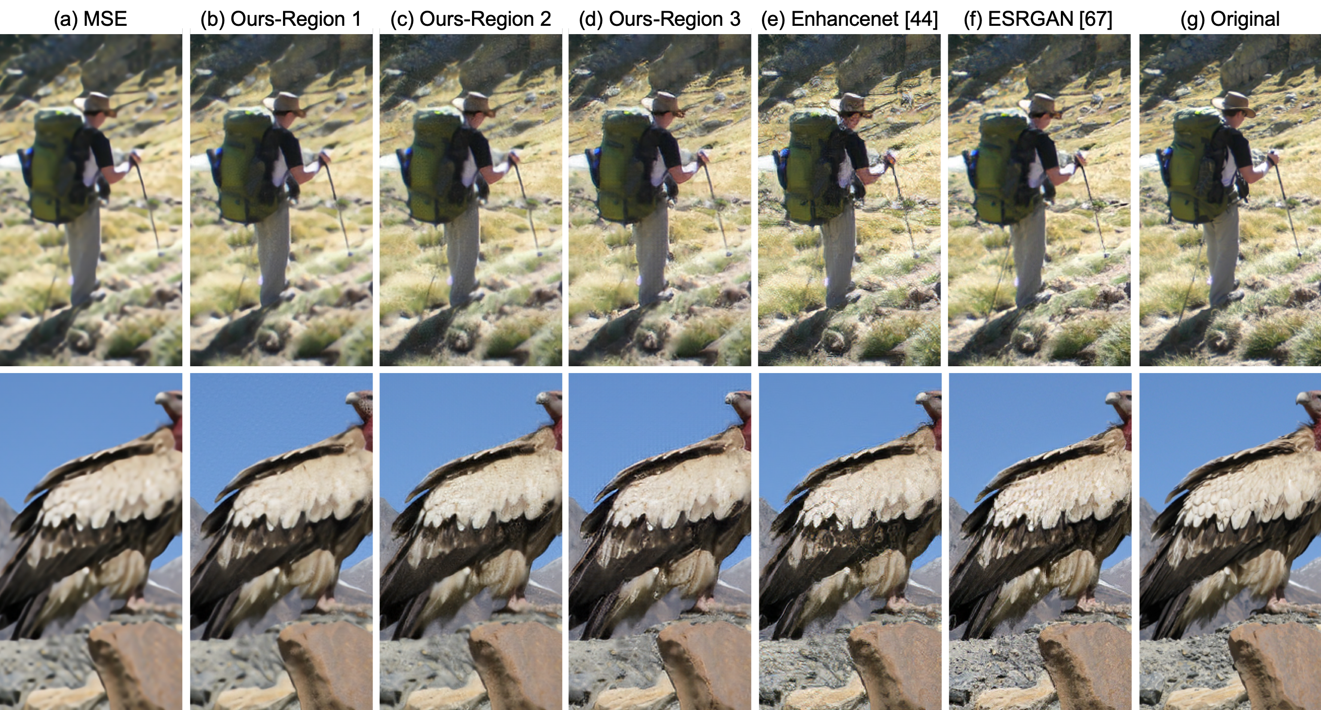
Figure 16: Results of DBPN with perceptual loss compare with other methods.

We show qualitative results from our method which is shown in Fig. 16. It can be seen that there are significant improvement on high quality texture on each region compare to MSE-optimized SR image. ESRGAN [63], the winner of PIRM2019 on Region 3, gets the best perceptual results among other methods. However, our proposal contains less noise among other methods (the smallest RMSE) while maintaining good perceptual quality on Region 3.

7 Conclusion

We have proposed Deep Back-Projection Networks for Single Image Super-resolution which is the winner of two single image SR challenge (NTIRE2018 and PIRM2018). Unlike the previous methods which predict the SR image in a feed-forward manner, our proposed networks focus to directly increase the SR features using multiple up- and down-sampling stages and feed the error predictions on each depth in the networks to revise the sampling results, then, accumulates the self-correcting features from each upsampling stage to create SR image. We use error feedbacks from the up- and down-scaling steps to guide the network to achieve a better result. The results show the effectiveness of the proposed network compares to other state-of-the-art methods. Moreover, our proposed network successfully outperforms other state-of-the-art methods on large scaling factors such as $8\times$ enlargement. We also show that DBPN can be modified into several variants to follow the latest deep learning trends to improve its performance.

Muhammad Haris Muhammad Haris received S. Kom (Bachelor of Computer Science) from the Faculty of Computer Science, University of Indonesia, Depok, Indonesia, in 2009. Then, he received the M. Eng and Dr. Eng degree from Department of Intelligent Interaction Technologies, University of Tsukuba, Japan, in 2014 and 2017, respectively, under the supervision of Dr. Hajime Nobuhara. He worked as postdoctoral fellow in Intelligent Information Media Laboratory, Toyota Technological Institute with Prof. Norimichi Ukita. Currently, he is working as AI Research Manager at BukaLapak.

Greg Shakhnarovich Greg Shakhnarovich has been faculty member at TTI-Chicago since 2008. He received his BSc degree in Computer Science and Mathematics from the Hebrew University in Jerusalem, Israel, in 1994, and a MSc degree in Computer Science from the Technion, Israel, in 2000. Prior to joining TTIC Greg was a Postdoctoral Research Associate at Brown University, collaborating with researchers at the Computer Science Department and the Brain Sciences program there. Greg’s research interests lie broadly in computer vision and machine learning.

Norimichi Ukita Norimichi Ukita is a professor at the graduate school of engineering, Toyota Technological Institute, Japan (TTI-J). He received the B.E. and M.E. degrees in information engineering from Okayama University, Japan, in 1996 and 1998, respectively, and the Ph.D degree in Informatics from Kyoto University, Japan, in 2001. After working for five years as an assistant professor at NAIST, he became an associate professor in 2007 and moved to TTIJ in 2016. He was a research scientist of Precursory Research for Embryonic Science and Technology, Japan Science and Technology Agency (JST), during 2002 - 2006. He was a visiting research scientist at Carnegie Mellon University during 2007-2009. He currently works also at the Cybermedia center of Osaka University as a guest professor. His main research interests are object detection/tracking and human pose/shape estimation. He is a member of the IEEE.

References

- [1] G. Huang, Z. Liu, L. van der Maaten, and K. Q. Weinberger, “Densely connected convolutional networks,” in Proceedings of the IEEE Conference on Computer Vision and Pattern Recognition, 2017.
- [2] K. He, X. Zhang, S. Ren, and J. Sun, “Deep residual learning for image recognition,” arXiv preprint arXiv:1512.03385, 2015.
- [3] E. L. Denton, S. Chintala, R. Fergus et al., “Deep generative image models using a laplacian pyramid of adversarial networks,” in Advances in neural information processing systems, 2015, pp. 1486–1494.
- [4] A. Shrivastava, T. Pfister, O. Tuzel, J. Susskind, W. Wang, and R. Webb, “Learning from simulated and unsupervised images through adversarial training,” in Proceedings of the IEEE Conference on Computer Vision and Pattern Recognition, 2017.
- [5] G. Larsson, M. Maire, and G. Shakhnarovich, “Fractalnet: Ultra-deep neural networks without residuals,” arXiv preprint arXiv:1605.07648, 2016.
- [6] A. Radford, L. Metz, and S. Chintala, “Unsupervised representation learning with deep convolutional generative adversarial networks,” arXiv preprint arXiv:1511.06434, 2015.
- [7] E. Ilg, N. Mayer, T. Saikia, M. Keuper, A. Dosovitskiy, and T. Brox, “Flownet 2.0: Evolution of optical flow estimation with deep networks,” in IEEE Conference on Computer Vision and Pattern Recognition (CVPR), Jul 2017.
- [8] J. Johnson, A. Alahi, and L. Fei-Fei, “Perceptual losses for real-time style transfer and super-resolution,” in European Conference on Computer Vision. Springer, 2016, pp. 694–711.
- [9] X. Tao, H. Gao, R. Liao, J. Wang, and J. Jia, “Detail-revealing deep video super-resolution,” in Proceedings of the IEEE International Conference on Computer Vision, Venice, Italy, 2017, pp. 22–29.
- [10] M. S. Sajjadi, R. Vemulapalli, and M. Brown, “Frame-recurrent video super-resolution,” in Proceedings of the IEEE Conference on Computer Vision and Pattern Recognition, 2018, pp. 6626–6634.
- [11] M. Haris, M. R. Widyanto, and H. Nobuhara, “Inception learning super-resolution,” Appl. Opt., vol. 56, no. 22, pp. 6043–6048, Aug 2017.
- [12] J. Kim, J. Kwon Lee, and K. Mu Lee, “Accurate image super-resolution using very deep convolutional networks,” in Proceedings of the IEEE Conference on Computer Vision and Pattern Recognition, June 2016, pp. 1646–1654.
- [13] W.-S. Lai, J.-B. Huang, N. Ahuja, and M.-H. Yang, “Deep laplacian pyramid networks for fast and accurate super-resolution,” in IEEE Conferene on Computer Vision and Pattern Recognition, 2017.
- [14] Y. Tai, J. Yang, and X. Liu, “Image super-resolution via deep recursive residual network,” in Proceedings of the IEEE Conference on Computer Vision and Pattern Recognition, 2017.
- [15] Y. Zhang, K. Li, K. Li, L. Wang, B. Zhong, and Y. Fu, “Image super-resolution using very deep residual channel attention networks,” in Proceedings of the European Conference on Computer Vision (ECCV), 2018, pp. 286–301.
- [16] S.-J. Park, H. Son, S. Cho, K.-S. Hong, and S. Lee, “Srfeat: Single image super-resolution with feature discrimination,” in Proceedings of the European Conference on Computer Vision (ECCV), 2018, pp. 439–455.
- [17] C. Dong, C. C. Loy, K. He, and X. Tang, “Image super-resolution using deep convolutional networks,” IEEE transactions on pattern analysis and machine intelligence, vol. 38, no. 2, pp. 295–307, 2016.
- [18] C. Dong, C. C. Loy, and X. Tang, “Accelerating the super-resolution convolutional neural network,” in European Conference on Computer Vision. Springer, 2016, pp. 391–407.
- [19] W. Shi, J. Caballero, F. Huszár, J. Totz, A. P. Aitken, R. Bishop, D. Rueckert, and Z. Wang, “Real-time single image and video super-resolution using an efficient sub-pixel convolutional neural network,” in Proceedings of the IEEE Conference on Computer Vision and Pattern Recognition, 2016, pp. 1874–1883.
- [20] J. Kim, J. Kwon Lee, and K. Mu Lee, “Deeply-recursive convolutional network for image super-resolution,” in Proceedings of the IEEE Conference on Computer Vision and Pattern Recognition, 2016, pp. 1637–1645.
- [21] S. Schulter, C. Leistner, and H. Bischof, “Fast and accurate image upscaling with super-resolution forests,” in Proceedings of the IEEE Conference on Computer Vision and Pattern Recognition, 2015, pp. 3791–3799.
- [22] M. Haris, M. R. Widyanto, and H. Nobuhara, “First-order derivative-based super-resolution,” Signal, Image and Video Processing, vol. 11, no. 1, pp. 1–8, 2017.
- [23] R. Timofte, V. De Smet, and L. Van Gool, “A+: Adjusted anchored neighborhood regression for fast super-resolution,” in Asian Conference on Computer Vision. Springer, 2014, pp. 111–126.
- [24] M. Haris, T. Watanabe, L. Fan, M. R. Widyanto, and H. Nobuhara, “Superresolution for uav images via adaptive multiple sparse representation and its application to 3-d reconstruction,” IEEE Transactions on Geoscience and Remote Sensing, vol. 55, no. 7, pp. 4047–4058, July 2017.
- [25] D. J. Felleman and D. C. Van Essen, “Distributed hierarchical processing in the primate cerebral cortex.” Cerebral cortex (New York, NY: 1991), vol. 1, no. 1, pp. 1–47, 1991.
- [26] D. J. Kravitz, K. S. Saleem, C. I. Baker, L. G. Ungerleider, and M. Mishkin, “The ventral visual pathway: an expanded neural framework for the processing of object quality,” Trends in cognitive sciences, vol. 17, no. 1, pp. 26–49, 2013.
- [27] V. A. Lamme and P. R. Roelfsema, “The distinct modes of vision offered by feedforward and recurrent processing,” Trends in neurosciences, vol. 23, no. 11, pp. 571–579, 2000.
- [28] M. Irani and S. Peleg, “Motion analysis for image enhancement: Resolution, occlusion, and transparency,” Journal of Visual Communication and Image Representation, vol. 4, no. 4, pp. 324–335, 1993.
- [29] S. Dai, M. Han, Y. Wu, and Y. Gong, “Bilateral back-projection for single image super resolution,” in Multimedia and Expo, 2007 IEEE International Conference on. IEEE, 2007, pp. 1039–1042.
- [30] B. Lim, S. Son, H. Kim, S. Nah, and K. M. Lee, “Enhanced deep residual networks for single image super-resolution,” in The IEEE Conference on Computer Vision and Pattern Recognition (CVPR) Workshops, July 2017.
- [31] M. Haris, G. Shakhnarovich, and N. Ukita, “Deep back-projection networks for super-resolution,” in Proceedings of the IEEE Conference on Computer Vision and Pattern Recognition, 2018.
- [32] R. Timofte, S. Gu, J. Wu, L. Van Gool, L. Zhang, M.-H. Yang, M. Haris, G. Shakhnarovich, N. Ukita et al., “Ntire 2018 challenge on single image super-resolution: Methods and results,” in Computer Vision and Pattern Recognition Workshops (CVPRW), 2018 IEEE Conference on, 2018.
- [33] Y. Blau, R. Mechrez, R. Timofte, T. Michaeli, and L. Zelnik-Manor, “2018 pirm challenge on perceptual image super-resolution,” arXiv preprint arXiv:1809.07517, 2018.
- [34] Y. Zhang, Y. Tian, Y. Kong, B. Zhong, and Y. Fu, “Residual dense network for image super-resolution,” in The IEEE Conference on Computer Vision and Pattern Recognition (CVPR), 2018.
- [35] J. Carreira, P. Agrawal, K. Fragkiadaki, and J. Malik, “Human pose estimation with iterative error feedback,” in Proceedings of the IEEE Conference on Computer Vision and Pattern Recognition, 2016, pp. 4733–4742.
- [36] S. Ross, D. Munoz, M. Hebert, and J. A. Bagnell, “Learning message-passing inference machines for structured prediction,” in Computer Vision and Pattern Recognition (CVPR), 2011 IEEE Conference on. IEEE, 2011, pp. 2737–2744.
- [37] Z. Tu and X. Bai, “Auto-context and its application to high-level vision tasks and 3d brain image segmentation,” IEEE Transactions on Pattern Analysis and Machine Intelligence, vol. 32, no. 10, pp. 1744–1757, 2010.
- [38] K. Li, B. Hariharan, and J. Malik, “Iterative instance segmentation,” in Proceedings of the IEEE Conference on Computer Vision and Pattern Recognition, 2016, pp. 3659–3667.
- [39] A. R. Zamir, T.-L. Wu, L. Sun, W. Shen, J. Malik, and S. Savarese, “Feedback networks,” arXiv preprint arXiv:1612.09508, 2016.
- [40] A. Shrivastava and A. Gupta, “Contextual priming and feedback for faster r-cnn,” in European Conference on Computer Vision. Springer, 2016, pp. 330–348.
- [41] W. Lotter, G. Kreiman, and D. Cox, “Deep predictive coding networks for video prediction and unsupervised learning,” arXiv preprint arXiv:1605.08104, 2016.
- [42] I. Goodfellow, J. Pouget-Abadie, M. Mirza, B. Xu, D. Warde-Farley, S. Ozair, A. Courville, and Y. Bengio, “Generative adversarial nets,” in Advances in neural information processing systems, 2014, pp. 2672–2680.
- [43] C. Ledig, L. Theis, F. Huszár, J. Caballero, A. Cunningham, A. Acosta, A. Aitken, A. Tejani, J. Totz, Z. Wang et al., “Photo-realistic single image super-resolution using a generative adversarial network,” in IEEE Conference on Computer Vision and Pattern Recognition (CVPR), Jul 2017.
- [44] M. S. Sajjadi, B. Schölkopf, and M. Hirsch, “Enhancenet: Single image super-resolution through automated texture synthesis,” arXiv preprint arXiv:1612.07919, 2016.
- [45] K. Simonyan and A. Zisserman, “Very deep convolutional networks for large-scale image recognition,” ICLR, 2015.
- [46] Y. Zhao, R.-G. Wang, W. Jia, W.-M. Wang, and W. Gao, “Iterative projection reconstruction for fast and efficient image upsampling,” Neurocomputing, vol. 226, pp. 200–211, 2017.
- [47] W. Dong, L. Zhang, G. Shi, and X. Wu, “Nonlocal back-projection for adaptive image enlargement,” in Image Processing (ICIP), 2009 16th IEEE International Conference on. IEEE, 2009, pp. 349–352.
- [48] R. Timofte, R. Rothe, and L. Van Gool, “Seven ways to improve example-based single image super resolution,” in Proceedings of the IEEE Conference on Computer Vision and Pattern Recognition, 2016, pp. 1865–1873.
- [49] C. Szegedy, W. Liu, Y. Jia, P. Sermanet, S. Reed, D. Anguelov, D. Erhan, V. Vanhoucke, and A. Rabinovich, “Going deeper with convolutions,” in Proceedings of the IEEE Conference on Computer Vision and Pattern Recognition, 2015, pp. 1–9.
- [50] K. He, X. Zhang, S. Ren, and J. Sun, “Delving deep into rectifiers: Surpassing human-level performance on imagenet classification,” in Proceedings of the IEEE International Conference on Computer Vision, 2015, pp. 1026–1034.
- [51] E. Agustsson and R. Timofte, “Ntire 2017 challenge on single image super-resolution: Dataset and study,” in The IEEE Conference on Computer Vision and Pattern Recognition (CVPR) Workshops, July 2017.
- [52] W.-S. Lai, J.-B. Huang, N. Ahuja, and M.-H. Yang, “Fast and accurate image super-resolution with deep laplacian pyramid networks,” IEEE transactions on pattern analysis and machine intelligence, 2018.
- [53] J. Li, F. Fang, K. Mei, and G. Zhang, “Multi-scale residual network for image super-resolution,” in Proceedings of the European Conference on Computer Vision (ECCV), 2018, pp. 517–532.
- [54] T. Dai, J. Cai, Y. Zhang, S.-T. Xia, and L. Zhang, “Second-order attention network for single image super-resolution,” in Proceedings of the IEEE Conference on Computer Vision and Pattern Recognition, 2019, pp. 11 065–11 074.
- [55] M. Bevilacqua, A. Roumy, C. Guillemot, and M.-L. A. Morel, “Low-complexity single-image super-resolution based on nonnegative neighbor embedding,” in British Machine Vision Conference (BMVC), 2012.
- [56] R. Zeyde, M. Elad, and M. Protter, “On single image scale-up using sparse-representations,” in Curves and Surfaces. Springer, 2012, pp. 711–730.
- [57] P. Arbelaez, M. Maire, C. Fowlkes, and J. Malik, “Contour detection and hierarchical image segmentation,” IEEE transactions on pattern analysis and machine intelligence, vol. 33, no. 5, pp. 898–916, 2011.
- [58] J.-B. Huang, A. Singh, and N. Ahuja, “Single image super-resolution from transformed self-exemplars,” in Proceedings of the IEEE Conference on Computer Vision and Pattern Recognition, 2015, pp. 5197–5206.
- [59] Y. Matsui, K. Ito, Y. Aramaki, A. Fujimoto, T. Ogawa, T. Yamasaki, and K. Aizawa, “Sketch-based manga retrieval using manga109 dataset,” Multimedia Tools and Applications, pp. 1–28, 2016.
- [60] Z. Wang, A. C. Bovik, H. R. Sheikh, and E. P. Simoncelli, “Image quality assessment: from error visibility to structural similarity,” Image Processing, IEEE Transactions on, vol. 13, no. 4, pp. 600–612, 2004.
- [61] X. Wang, K. Yu, C. Dong, and C. Change Loy, “Recovering realistic texture in image super-resolution by deep spatial feature transform,” in Proceedings of the IEEE Conference on Computer Vision and Pattern Recognition, 2018, pp. 606–615.
- [62] S. Vasu, N. Thekke Madam, and A. Rajagopalan, “Analyzing perception-distortion tradeoff using enhanced perceptual super-resolution network,” in Proceedings of the European Conference on Computer Vision (ECCV), 2018.
- [63] X. Wang, K. Yu, S. Wu, J. Gu, Y. Liu, C. Dong, Y. Qiao, and C. Change Loy, “Esrgan: Enhanced super-resolution generative adversarial networks,” in Proceedings of the European Conference on Computer Vision (ECCV), 2018.
- [64] M. Cheon, J.-H. Kim, J.-H. Choi, and J.-S. Lee, “Generative adversarial network-based image super-resolution using perceptual content losses,” in Proceedings of the European Conference on Computer Vision (ECCV), 2018.
- [65] P. Navarrete Michelini, D. Zhu, and H. Liu, “Multi–scale recursive and perception–distortion controllable image super–resolution,” in Proceedings of the European Conference on Computer Vision (ECCV), 2018.
- [66] J.-H. Choi, J.-H. Kim, M. Cheon, and J.-S. Lee, “Deep learning-based image super-resolution considering quantitative and perceptual quality,” arXiv preprint arXiv:1809.04789, 2018.
- [67] T. Vu, T. M. Luu, and C. D. Yoo, “Perception-enhanced image super-resolution via relativistic generative adversarial networks,” in Proceedings of the European Conference on Computer Vision (ECCV), 2018.
- [68] X. Luo, R. Chen, Y. Xie, Y. Qu, and C. Li, “Bi-gans-st for perceptual image super-resolution,” in Proceedings of the European Conference on Computer Vision (ECCV), 2018.
- [69] K. Purohit, S. Mandal, and A. Rajagopalan, “Scale-recurrent multi-residual dense network for image super-resolution,” in Proceedings of the European Conference on Computer Vision (ECCV), 2018.
- [70] A. Dosovitskiy and T. Brox, “Generating images with perceptual similarity metrics based on deep networks,” in Advances in Neural Information Processing Systems, 2016, pp. 658–666.
- [71] L. A. Gatys, A. S. Ecker, and M. Bethge, “Image style transfer using convolutional neural networks,” in Proceedings of the IEEE Conference on Computer Vision and Pattern Recognition, 2016, pp. 2414–2423.
- [72] C. Ma, C.-Y. Yang, X. Yang, and M.-H. Yang, “Learning a no-reference quality metric for single-image super-resolution,” Computer Vision and Image Understanding, vol. 158, pp. 1–16, 2017.
- [73] A. Mittal, R. Soundararajan, and A. C. Bovik, “Making a” completely blind” image quality analyzer.” IEEE Signal Process. Lett., vol. 20, no. 3, pp. 209–212, 2013.