Intelligent measurement analysis on single cell Raman images for the diagnosis of follicular thyroid carcinoma

Abstract

Inter-observer variability and cancer over-diagnosis are emerging clinical problems, and there is a strong necessity to support the standards histological and cytological evaluations by biochemical composition information. Over the past decades, there has been a very active research in the development of Raman spectroscopy techniques for oncological applications and large scale clinical diagnosis. A major issue that has received considerable interest in the Raman literature is the fact that variations in instrumental responses and intrinsic spectral backgrounds over different days of measurements or devices creates strong inconsistency of Raman intensity spectra over the various experimental condition, thus making the use of Raman spectroscopy on a large scale and reproductive basis difficult. We explore different methods to tackle this inconsistency and show that regular preprocessing methods such as baseline correction, normalization or wavelet transformation are inefficient on our datasets. We find that subtracting the mean background spectrum estimated by identifying non-cell regions in Raman images makes the data more consistent. As a proof of concept, we employ our single-cell Raman Imaging protocol to diagnosis challenging follicular lesions, that is known to be particularly difficult due to the lack of obvious morphological and cytological criteria for malignancy. We explore dimensionality reduction with both PCA and feature selection methods, and classification is then performed at the single cell level with standard classifiers such as k Nearest Neighbors or Random Forest. We investigate Raman hyperspectral images from FTC133, RO82W-1 and NthyOri 3-1 cell lines and show that the chemical information for the diagnosis is mostly contained in the cytoplasm. We also reveal some important wavenumber for malignancy, that can be associated mainly to lipids, cytochrome c and phenylalanine. We obtain cell classification test accuracies ranging from $80\text{\,}\%$ to $86\text{\,}\%$.

Introduction

Although histopathologic diagnosis nowadays represents the ultimate diagnostic method for many form of cancers [1], it sometimes suffers from great inter- and intra-observer variability and is also subjected to sampling errors even among the experts. In order to reduce the false positive or false negative rates in clinical diagnostics and thus avoid overtreatment or undertreatment, there is a strong necessity to support the histological and cytological evaluations by biochemical composition information. In the last fifteen years, numerous molecular analyses have been investigated, with the scope of reducing the diagnostic variability (e.g. immunohistochemistry [2], gene expression profiling [3], etc).

A typical example that would benefit greatly from new clinical tools is the diagnosis of follicular lesions of the thyroid [4], which is known to be particularly difficult due to the lack of obvious morphological and cytological criteria for malignancy [5]. The diagnosis of thyroid lesions have many variants [6], each involving different risks and necessary treatments for patients: Follicular Thyroid Carcinoma (FTC), Papillary Thyroid Carcinoma (PTC), Follicular variant of PTC (FVPTC), Undifferentiated Thyroid Carcinoma (UTC), Medullary Thyroid Carcinoma (MTC) and Follicular Adenoma (FA) (that is not malignant). Recent literature suggest that a growing part of the detected thyroid cancers are overdiagnosed and overtreated [7, 8], which indicates that a significant proportion of unnecessary surgical solutions and further treatment such as thyroidectomy and radiotherapy could be avoided by supporting the traditional Fine Needle Aspiration Cytology diagnosis (FNAC) of thyroid lesions with biochemical composition information.

In this context, Raman spectroscopy is very promising to increase diagnostic reliability as it is a non-destructive technique capable of providing high molecular specificity and sensitivity, while requiring minimal sample preparation [9]. In the last few decades, the number of Raman studies focused on oncology based problems, and more generally on various tissue and cellular pathologies, has been growing progressively [10, 11]. Particularly, there is a considerable clinical requirement for a noninvasive real-time Raman probe [12] that can perform accurate and repeatable measurement of pathological state. While Raman measurements for clinical applications are generally performed at the cellular level to diagnosis neoplastic tissues containing dozens to hundreds of cells, the excitation wavelength in the visible and near-infrared range also allow a higher spatial resolution and can provide hyperspectral Raman images of individual cells at the sub-cellular level [13, 14]. Extraction of chemical and spatial information of sub-cellular components in individual cells have the potential to give a more complete understanding of the underlying biological processes as well as better accuracies in clinical diagnosis. [15]

For a large scale clinical use, Raman measurements needs to be reliable and repeatable over a very wide range of experimental condition. However, a major issue of Raman spectroscopy is the fact that the intensity at each wavenumber is heavily influenced by experimental conditions, such as light scattering by instruments or unstable auto fluorescence from samples, leading to inconsistency of the Raman intensity spectra over different days of measurement or devices. This requires a robust calibration, preprocessing and postprocessing procedure to account for possible variations in the Raman measurements. While numerous processing methods are mentioned in literature [16, 17], there is still currently a lack of robust and reliable tool for clinical diagnosis with Raman spectroscopy [17].

In this study, we focus on the diagnosis of FTC vs NT on large dataset and aim at developing a general and reliable method to analyze spectral imaging data of cells and living tissues in a consistent and reproductive way. We analyze sub-cellular hyperspectral Raman images measured in different experimental condition over different months and highlight their inconsistency when preprocessed with standards approach such as wavelet decomposition or baseline correction. We tackle this issue by subtracting the mean background spectrum estimated by averaging spectra over non-cell regions in Raman images. The second part explore the chemical differences between FTC and NT, and reveal some important wavenumber for malignancy. We also highlight the organelle dependence in single cell classification performances.

Related work    Cytopathologic diagnosis by Fine Needle Aspiration biopsies (FNAC) is nowadays widely accepted as the initial step in the management of thyroid nodules [18, 19]. However, a significant number of cases (roughly $30\text{\,}\%$) are reported as follicular tumors of unknown malignant potential (FT-UMP) due to incomplete evidence of malignant features [20]. In this context, several teams have experimented the differentiation of thyroid follicular lesions with Raman spectroscopy to improve clinical diagnosis, utilizing both cell lines [15, 21, 22, 23] and tissue sections[24, 25]. Although they emphasized a lack of obvious spectral criteria for malignancy, feature extraction and dimensionality reduction methods enabled the obtention of good accuracies, ranging from 75% to 95% for the diagnosis of thyroid cancers. They however reported high variability of Raman spectra, especially for those who had performed measurement over different days and in various experimental conditions [24]. All of the mentioned works for Raman involve relatively small datasets, containing around 50 examples.

Regarding the analytic techniques for Raman spectra, an extensive review of preprocessing and postprocessing techniques methods are provided in [16, 17]. Standard methods include denoising, baseline correction and normalization. Denoising is usually performed with Singular Value Decomposition (SVD) [26] or Principal Component Analysis (PCA) [27], that can effectively reduce the spectra into a defined number of principal components. Baseline correction such as recursive Polynomial fitting (Polyfit) [28] or by Asymmetric Least Square smoothing (ALS)[29] are then commonly used to remove contribution from unknown fluorescent background, but they potentially introduce unintended artifacts and inevitably damage the information of low frequency components. Direct background subtraction with spectra measured from cell free reference sample are also an alternative to deal with the background [30], but these methods typically requires to measure additional samples prior to the measurement for each image. Finally, normalization is usually required to correct for sample and experimental variables. Because Raman spectra involve hundreds to thousands of wavenumbers, postprocessing generally start by selecting some specific wavenumbers or by applying dimensionality reduction methods such as PCA or ISOMAP [31]. Automated classification to determine whether an image (at either tissue or cellular level) belongs to a diseased tissue is then performed with standard supervised classifiers [5] such as nearest neighbors, linear discriminant analysis, support vector machines, etc.. Finally, advanced chemical information can be obtained by sub-cellular clustering analysis on Raman hyperspectral images[32, 15]. It allows the separation of individual cells into different clusters that can be chemically identified to specific biological markers by looking at the average spectra of that class.

One important step towards the sub-cellular study of hyperspectral Raman images is the segmentation of cellular structures. Popular methods are based on Kmean clustering, hierarchical agglomerative clustering and spectral phasor analysis [33], but these approaches are mostly limited to simple cases where cells are not packed together. While it is possible to deal with packed cell by looking at their nuclei and separate them based on the image intensity gradient [15], there is still a lack for fully automated segmentation methods of Raman hyperspectral images.

Our contribution    In this article, we describe an automated approach capable of classifying single cell Raman hyperspectral image data of FTC and Normal Thyroid (NT). We explore the inconsistencies of Raman data over different days of measurements and propose a background subtraction method by identifying and averaging non-cells regions in hyperspectral images. We then demonstrate that dimensionality reduction methods combined with simple classifiers such as k Nearest Neighbors (kNN) or Random Forest (RF) lead to up to $86\text{\,}\%$ test accuracy on our large dataset. We also provide detailed biochemical analysis by performing wavenumber selection to identify the relevant chemical compounds, and investigate the spectral information at the subcellular level. Finally, although this article demonstrates that these methods are successful for the diagnosis of cancer thyroid lesions, none of the methods we describe are specific to these lesions, and our approaches could easily be generalized to any Raman hyperspectral images applications.

Results

Hyperspectral Raman images were obtained from FTC133, RO82W-1 and Nthy3-1 cell lines. The detailed description of sample preparation and Raman measurements are given in the Methods section. In short, measurements were performed by two independent teams with two different Raman devices, at different days over a year. Our study involve 86 hyperspectral images taken at 16 different dates by two independent teams.

Hyperspectral Raman images data consist of three dimensional matrices, the first two axis corresponding to the pixel position and the third axis being the Raman intensity spectrum at that pixel. One image contains roughly $80\,000\text{\,}$ spectra with 1000 wavenumbers each, in the range of 700 - $3000\text{\,}\mathrm{c}\mathrm{m}^{-1}$. Two-dimensional image frames at wavenumbers corresponding to Cytochrome c ($750\text{\,}\mathrm{c}\mathrm{m}^{-1}$), proteins (Amide I, $1681\text{\,}\mathrm{c}\mathrm{m}^{-1}$), and lipids ($\text{CH}_{2}$ bending at $2852\text{\,}\mathrm{c}\mathrm{m}^{-1}$), are shown for representative hyperspectral images Figure.1.

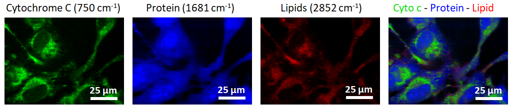
Figure 1: Representative Hyperspectral Raman image: Two-dimensional image frames at wavenumbers corresponding to Cytochrome C ($750\text{\,}\mathrm{c}\mathrm{m}^{-1}$), proteins (amide I at $1681\text{\,}\mathrm{c}\mathrm{m}^{-1}$), and lipids ($\text{CH}_{2}$ bending at $2852\text{\,}\mathrm{c}\mathrm{m}^{-1}$).

Cell segmentation and isolation

Under the working assumption that cell regions are brighter than their non-cell counterparts in the high wavenumber region, differentiation of cell regions from non-cell regions is performed by K-means superpixel clustering (See methods for details). However, as shown on Figure.2, the relatively high cell density in some Raman images requires manual segmentation to correctly isolate the cells. Note that the relatively small dataset, the wide variety of cell shape and the complex boundary decision for high cell density images makes automated segmentation of cellular structure particularly challenging. After superpixel segmentation of the images[15] and cell regions isolation, we are left with 365 Nthy3-1 cells, 314 FTC133 cells and 141 RO82W-1 cells, (Total 820 cells), each containing roughly 1000 spectra.

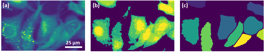
Figure 2: Representative Hyperspectral Raman image: (a) Two-dimensional image frames of unprocessed spectra averaged over the entire wavenumber range. (b) Four brightest clusters after spectral K-means clustering in the high wavenumber region with 8 clusters. (c) Cells obtained after manual segmentation

Raman spectra preprocessing and inconsistencies over different days of measurements

The gold standard for Raman spectra preprocessing involve denoising, baseline correction and normalization. Although these three steps have proven numerous times to be enough to extract reliable spectral data over various experimental conditions, the obtained spectra may still differ due to some uncontrolled artifacts. Fortunately, these inconsistencies are generally negligible relatively to the differences over the spectral classes for classification.

We applied standard preprocessing techniques on our datasets: each spectrum has undergone denoising with SVD, baseline correction with $7^{\text{th}}$ order Polyfit, and area normalization (see methods for details). Figure.3a,3b plot the average spectra obtained after preprocessing. Note that the silent region (1800-$2800\text{\,}\mathrm{c}\mathrm{m}^{-1}$) was cropped due to the lack of relevant biological markers in that wavenumber range. For visualization purpose, dimensionality reduction is performed by Principal Component Analysis (PCA) [27], which is a dimension-reduction tool that can be used to reduce a large set of variables to a smaller set that still explain most of the variability in the data. A scatter plot of the first two principal components of each superpixel spectrum labeled as their malignancy, date, and place respectively is given Figures.3c, 3d, 3e. From these plots we notice considerable differences between measurements performed with different Raman devices (3a,3c), but also at various days from the same team (3b,3d).

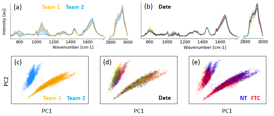
Figure 3: Raman data after denoising, $7^{\text{th}}$ order polyfit baseline correction and normalization. (a) Average Raman spectra measured from team 1 and team 2.(b) Average spectra taken at different dates from team 2. (c,d,e) are scatter plot of the first two principal components of each pixel spectrum labeled as their malignancy, date, and place respectively. The first two PCs contains roughly 77% of the spectral explained variance.

In particular, large spectral differences between teams 1 and 2 are found in the wavenumber range where non cellular components show major contributions (water and optical components at $750-$850\text{\,}\mathrm{c}\mathrm{m}^{-1}$$ and $1000-$1150\text{\,}\mathrm{c}\mathrm{m}^{-1}$$) (Figure.3a). This indicates that the differences between the two teams mainly comes from non-cellular signals, which is mostly determined by the experimental setup that is used for the measurements. As for the differences of the Raman intensity signal measured at different days on the same device, variability in both the degree of optical alignment and substrate condition may also produce relatively large variations in the non-cellular component regions (Figure.3b). In general, it seems like the notable variability among different days and setups mainly come from the cellular-to-noncellular signal ratio.

Regrouping the data with non cell region subtraction

Previous research has shown that the preprocessing methods presented above are applicable for measurements taken within the same day (without turning off the laser and thus changing optical conditions), and that there is a significant distinction between FTC and NT spectra [15]. More importantly, we found that these differences are consistent when the dataset are treated separately, which seems to indicate that Nthy cells are chemically relatively stable to FTC cells over different days.

To deal with the inconsistencies in the cellular-to-noncellular signal ratio, we propose to subtract the background estimated by averaging the spectra from non-cell regions, that typically contains the spectral contribution from both instrument response and sample fluorescence. As the area defined as background and non-background might varies through images due to differences in the cell density, non-cell regions are identified by defining a threshold on the high wavenumber region to ensure the consistency of background subtraction through different images, see method for a complete description of the procedure. Figure.4 show the estimated cell and non-cell region, and the corresponding average spectra. The obtained spectra after background subtraction and offset correction are plotted Figure.5.

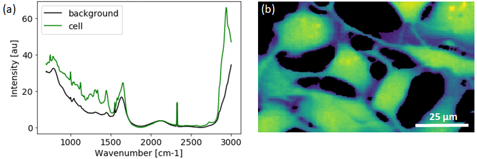
Figure 4: Non cell region subtraction protocol on a representative Raman image. (a) Mean spectra averaged over cell and background regions. (b) Two-dimensional image frames of unprocessed spectra averaged over the high wavenumber range, with the area corresponding to background region being colored in black.

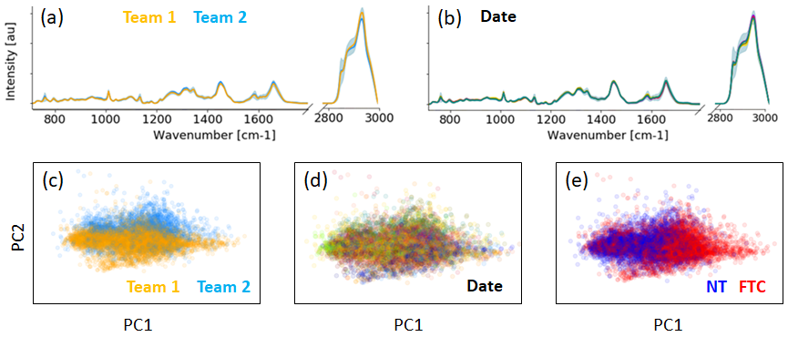
Figure 5: Raman data after non cell region subtraction, SVD denoising, $7^{\text{th}}$ order polyfit baseline correction and normalization. (a) Average Raman spectra measured from team 1 and team 2.(b) Average spectra taken at different dates from team 1. (c,d,e) are scatter plot of the first two principal components of each superpixel spectrum labeled as their malignancy, date, and place respectively. The first two PCs contains roughly 88% of the spectral explained variance.

While methods involving the subtraction of background spectra are not new, they typically require the measurement of additional reference samples prior to the actual measurement [30]. Our method, on the other hand, estimate the background spectra directly from the non cell regions in hyperspectral Raman images and does not requires any additional measurement. As emphasized by the results shown Figure.5, our protocol perform relatively well and makes the measurement more consistent.

Earth mover’s distance between distributions

As a tool to quantify how the measurements at different days differ from each other, and how subtraction from non cell regions improve their consistency, the Earth Mover’s Distance (EMD) [34] is a suitable metric to measure distances between two discrete distributions. In short, it reflects the minimal amount of work that must be performed to transform one distribution into the other by moving “distribution mass” around. Some advantage of EMD relatively to other measures like the Kullback–Leibler divergence is that it is symmetric, finite, and does not require any preliminary probability distribution computation. Generalization of the EMD distance to multiple distributions is done by averaging over the distances of all possible pair of distribution. The python library Optimal Transport[35] was used in our work, details are given in the method section. Table.1 shows the computed distance between different groups in the PC1-PC2 space and emphasizes the benefit of non cell region subtraction on our dataset.

Table 1: Computed EMD distance between different groups before and after non cell region subtraction. "Dates NT" and "Dates FTC" corresponds to the case where each distribution correspond to one date of measurement of NT and FTC respectively. "NT vs FTC" is the distance between the FTC and NT distribution, all date combined.

	Without backgroung subtraction			With backgroung subtraction
Place	Dates NT	Dates FTC	NT vs FTC	Dates NT	Dates FTC	NT vs FTC
Both combined	13.4	8.55	1.3	1.4	1.2	2.1
Team 1 only	1.9	0.8	1.1	0.65	0.68	2.1
Team 2 only	5.2	1.8	2.1	1.48	1.04	2.1

Apart from the obvious differences between the measurements of team 1 and team 2 without background subtraction, the EMD distance is still significantly higher for measurement taken by the same team relatively to the one of FTC vs NT, which indicate that the spectral inconsistency over different day of measurement are more significant than the spectral distinction between FTC and NT, meaning that the standard preprocessing methods presented in the first part of our work are not suitable for our FTC/NT diagnosis on our datasets. On the other hand, The EMD distance after non cell region subtraction for different dates and places are always smaller than the EMD distance between FTC and NT, which reflect the efficiency of our procedure.

Postprocessing and Raman peaks

After making sure that our data are consistent through different days, we can combine all the measurements together and study the spectral properties to a obtain detailed biochemical profile associated to each pixel in the Raman images. The Raman spectrum averaged over all pixels is shown below Fig.6. Note that the wavenumber region 700-$1800\text{\,}\mathrm{c}\mathrm{m}^{-1}$ was increased by a factor of 4 to ease the presentation, and that the silent region (1800-$$2800\text{\,}\mathrm{c}\mathrm{m}^{-1}$)$ was cropped due to the lack of relevant biological markers in that wavenumber range.

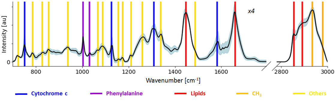
Figure 6: Raman spectrum averaged over all pixels within all images, the gray area is the one sigma variance. Major peaks in the spectrum are emphasized with vertical lines, colored according to their main chemical significance.

The broad contributions in the wavenumber ranges (700-$1800\text{\,}\mathrm{c}\mathrm{m}^{-1}$) and (2800-$3000\text{\,}\mathrm{c}\mathrm{m}^{-1}$) indicates the presence of a very wide variety of proteins and lipids [36, 25], that are typically contained in cellular tissues. The main contributions in the Raman spectra of Nthy3-1, FTC133 and RO82W1 cell lines (Fig.6) are summarized Table.2. The most noticeable peaks are:

• Broad contribution at (1410-$$1470\text{\,}\mathrm{c}\mathrm{m}^{-1}$)$ and (2800-$2900\text{\,}\mathrm{c}\mathrm{m}^{-1}$), indicating the presence $\text{CH}_{2}$ bending and stretching, along with (1630-$1700\text{\,}\mathrm{c}\mathrm{m}^{-1}$) for C=C stretching, mostly contained in lipids.[37]

• Broad contribution at (2900-$$3000\text{\,}\mathrm{c}\mathrm{m}^{-1}$)$ indicating the presence of $\text{CH}_{3}$ stretching, typically contained in the vast majority of biological compounds.

• Narrow peak at $750\text{\,}\mathrm{c}\mathrm{m}^{-1}$,$1127\text{\,}\mathrm{c}\mathrm{m}^{-1}$,$1314\text{\,}\mathrm{c}\mathrm{m}^{-1}$,$1585\text{\,}\mathrm{c}\mathrm{m}^{-1}$ associated to vibrational modes of Cytochromes [38] in the mitochondria.

• Strong and narrow peak at $1003\text{\,}\mathrm{c}\mathrm{m}^{-1}$ corresponding to Phenylalanine (C-C) stretching. [39]

Table 2: Assignment of the Major Peaks in the Raman Spectra of FTC and NT cell lines.
$\beta$ = bending; $\nu$ = stretching (s = symmetric; as = asymmetric);

Wavenumber peak ($\pm$5\text{\,}\mathrm{c}\mathrm{m}^{-1}$$)	Amino acids [39, 25] (building blocks of proteins)	Lipids[37] (Fatty acids, Triacylglycerols)	Others (DNA [40], Cytochromes [38])
723			Adenine (DNA)
750	Tryptophan		Cytochrome c
786			Cytosine (DNA)
828	Tyrosine
855	Tyrosine, Proline
938	Proline
1004	Phenylalanine
1032	Phenylalanine
1068 and 1089	$\nu(\text{C}-\text{C})$	$\nu(\text{C}-\text{C})$
1127	$\nu(\text{C}-\text{N})$		Cytochrome c
1155	$\nu(\text{C}-\text{C})$ and $\nu(\text{C}-\text{N})$	$\nu(\text{C}-\text{C})$
1175	Tyrosine
1211	Amide III
1265	Amide III
1310	Tryptophan		Cytochrome c
1339	Tryptophan, Amide III
1447	$\nu(\text{C}-\text{H})$	$\beta(\text{CH}_{2}),\beta(\text{CH}_{3})$
1485			Adenine (DNA)
1581	Phenylalanine, Proline		Cytochrome c
1659	Amide I	$\nu_{\text{s}}(\text{C}=\text{C})$
2854		$\nu_{\text{s}}(=\text{CH}_{2})$
2890		$\nu_{\text{as}}(=\text{CH}_{2})$
2934	$\nu_{\text{s}}(=\text{CH}_{3})$	$\nu_{\text{s}}(=\text{CH}_{3})$	$\nu_{\text{s}}(=\text{CH}_{3})$
2979	$\nu_{\text{as}}(=\text{CH}_{3})$	$\nu_{\text{as}}(=\text{CH}_{3})$	$\nu_{\text{as}}(=\text{CH}_{3})$

Organelle dependence, Nucleus vs Cytoplasm

As a first step for the analysis of the cell lines, we separate cell regions into two distinct categories: nucleus and cytoplasm, that differ in their spectral response notably in the lipid region (Figure.7a) . Differentiation of nucleus regions relatively to cytoplasm region is done by K-means clustering on the CH2 stretching region $2842-$2910\text{\,}\mathrm{c}\mathrm{m}^{-1}$$, see method for detailed description of the procedure.

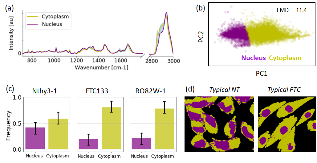
Figure 7: Organelle analysis of Nthy3-1, FTC133 and RO82W-1 cell lines. (a)Average spectra from Nucleus Region and Cytoplasm region respectively (b)Nucleus and Cytoplasm pixel spectra in the PC1-PC2 space (contains 88% of the information). (c)Median Nucleus and Cytoplasm fraction population in individual FTC cells and NT cells, error bar are the first and third quartile. (d)Typical FTC and NT Raman image with cell region colored according to their class.

From Figure 7c, we immediately observe that NT cells contains more nucleus region (40%) than FTC cells (20 %), which suggest that NT cells have on average a bigger nucleus than FTC. Clinical diagnosis of FTC by histological methods is however well known to be challenging do to the lack of obvious morphological features for malignancy [5], and the difference that we obverse is probably unique to the Nthy3-1 cell line rather than an actual general morphological difference in clinical applications. It is possible that such difference comes from the SV40 large T antigen protein that was artificially introduced in Nthy cells for immortalization. In our analysis, we have to make sure that good classification accuracy comes from an actual chemical difference in the cell rather than just the fact that NT has bigger nucleus than FTC.

As for further analysis, Fig.8.I, 8.II and 8.III showcase the FTC vs NT spectral difference averaged over the whole cell, nucleus region only, and cytoplasm region only respectively. As emphasizes the scatter plot in the PC1-PC2 space, the distinction between FTC and NT is very poor for nucleus regions, which indicates that NT and FTC nucleus does not contain any relevant chemical difference for FTC clinical diagnosis. As expected, the spectral difference at wavenumbers $750\text{\,}\mathrm{c}\mathrm{m}^{-1}$, $1127\text{\,}\mathrm{c}\mathrm{m}^{-1}$, $1314\text{\,}\mathrm{c}\mathrm{m}^{-1}$ and $1585\text{\,}\mathrm{c}\mathrm{m}^{-1}$ is increased for cytoplasm region relatively to whole cell region, because nucleus regions does not contain a weak cytochrome c contribution.

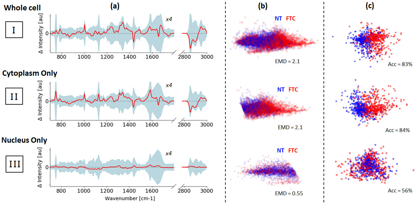
Figure 8: FTC vs NT for [I] the whole cell, [II] cytoplasm region only, [III] nucleus region only. (a) Average difference spectra $I(\text{NT})-I(\text{FTC})$, (b) pixel-wise PC1-PC2 (contains 88% of the information) scatter plot colored according to their malignancy along with the computed EMD distance between the two distributions, (c) scatter plot in the PC1-PC2 space, with each point corresponding to the average cell spectra over the region of interest (whole cell, cytoplasm, nucleus), classification accuracy by 10Nearest Neighbors is also given

We also performed a simple 10 Nearest Neighbor classification on the first 5 Principal Components (PCs) to check for the classification performances. Three spectra were produced for each cell by averaging over all the single-pixel located within the region assigned to the cell, cytoplasm and nucleus respectively. The results are summarized Table.3 We observe that the classification accuracy is similar for whole cell and cytoplasm only regions, but very poor for nucleus only regions. This is in agreement with the difference spectra and pixel-wise PC1-PC2 plot Fig.8a and Fig.8b.

Table 3: Cellular classification accuracy, AUC and F1 score with a 10 Nearest Neighbor classifier on the first 5 Principal Components of the average cellular spectra, computed by considering the whole cell, cytoplasm region only and nucleus region only. The number in parenthesis is the number of cells involved in the classification

	Full cell	Cytoplasm only	Nucleus Only
Nthy3-1 (365)	83%	85%	54%
FTC133 (314)	80%	78%	59%
RO82W-1 (141)	88%	93%	55%
Total Acc (820)	83%	84%	56%
Total F1 score	0.84	0.85	0.58
Total AUC	0.90	0.93	0.60

FTC/NT spectral differentiation in the cytoplasm

To make sure that good classification accuracy comes from an actual chemical difference in the cell rather than just the fact that NT has bigger nucleus than FTC, we discard the nucleus region and focus our analysis on cytoplasm regions only. After making sure that our data are consistent through different days, and that the variation in the nucleus size will not affect the classification, we can study the spectral differences between FTC and NT cell lines for clinical diagnosis. Figure.9a plot the mean FTC and NT spectra averaged over cytoplasm region over all images after non cell region subtraction, offset correction, and area normalization for the three cell lines FTC133, RO82W-1 and NthyOri 3-1.

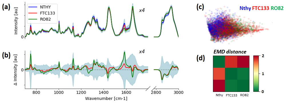
Figure 9: Cytoplasm processed (a) mean spectra of pixel from each cell line and (b) their difference with NT $\Delta I=I(\text{Nthy})-I(\text{FTC133})$, colored area is 1-sigma variance. (c) pixel spectra from different cell lines in the PC1-PC2 space (contains 88% of the information). (d) EMD distance matrix between cell lines in PC1-PC2 space

As emphasized by the EMD distance matrix between the three cell lines Figure.9d, RO82W-1 and FTC133 distributions are close to each other in the PC1-PC2 space relatively to Nthy. Note that the distance between FTC133 and RO82W-1 (0.5) is smaller than the average EMD between different dates (1.2). The spectral difference with Nthy Figure.9b also shows that FTC and RO82 have similar trend, although the one from RO82W-1 being more pronounced than FTC133.

From the difference spectra Figure.9b, we observe that despite their similarities, the cellular spectra of FTC and NT differ significantly at several important wavenumbers:

• Most notably, we observe an increased FTC intensity in the regions corresponding to $\text{CH}_{2}$ bending, C=C stretching and $\text{CH}_{2}$ stretching ($1440\text{\,}\mathrm{c}\mathrm{m}^{-1}$, $1650\text{\,}\mathrm{c}\mathrm{m}^{-1}$, 2800-$2900\text{\,}\mathrm{c}\mathrm{m}^{-1}$ respectively), suggesting a relative concentration increase of lipids in FTC cells, which is in agreement with literature reports of increased lipid activity in cancers [41].

• We also distinguish in FTC cells a significant decreased intensity in cytochrome c ($750\text{\,}\mathrm{c}\mathrm{m}^{-1}$,$1127\text{\,}\mathrm{c}\mathrm{m}^{-1}$,$1314\text{\,}\mathrm{c}\mathrm{m}^{-1}$,$1585\text{\,}\mathrm{c}\mathrm{m}^{-1}$). One possible interpretation is that FTC cells tends to breathe more than NT cells, and thus oxidize more cytochrome c, that has a different (and weaker) response in the Raman signal and thus reduce the cytochrome c peak intensity.

• Finally, we see in FTC cells a decreasing Phenylalanine ($1003\text{\,}\mathrm{c}\mathrm{m}^{-1}$) and Tryptophan ($1337\text{\,}\mathrm{c}\mathrm{m}^{-1}$) intensity, as well as a significant decrease in $\text{CH}_{3}$ (2900-$2900\text{\,}\mathrm{c}\mathrm{m}^{-1}$). Which would indicate that NT cells contains on average more proteins than FTC cells.

It has been reported that there is no significant biochemical difference between SV40 transfected bone cell line and primary bone cells [42]. As a result, it is unlikely that the spectral difference between FTC and NT is due to the SV40 large T protein (that was artificially added to Nthy cells for immortalization). Previous literature on hyperspectral Raman images of thyroid tissues [24] emphasized an increased presence of carotenoids in FTC cells from tissues, these are however not significant in our dataset due to the insignificant contribution of carotenoids in our spectra ($1006\text{\,}\mathrm{c}\mathrm{m}^{-1}$, $1156\text{\,}\mathrm{c}\mathrm{m}^{-1}$, $1520\text{\,}\mathrm{c}\mathrm{m}^{-1}$).

Cellular classification and Wavenumber importance in the cytoplasm

A single spectrum was produced for each cell by averaging over all the single-pixel located within the region assigned to the cytoplasm of each cell. Because our Raman spectra involve around 1000 wavenumbers, we explored three different methods to apply dimensionality reduction to our dataset prior to the classification. In our case, the features correspond to the Raman intensity at each wavenumber.

• PCA[27] (Feature extraction) is a dimension-reduction tool that is used to reduce a large set of variables to a smaller set that still explain most of the variability in the data. Each PCs is a linear combination of all the wavenumbers, the first PC accounting for as much of the variability in the data as possible, and each succeeding component accounting for as much of the remaining variability as possible. While it usually build relevant features for classification and provide easy visualization of the data, it does not give any chemical information about the FTC diagnosis. Figure.10c scatter the first two principal components of each cell in our dataset, colored according to their malignancy, it gives a relatively good separation between FTC and NT.

• ANOVA (Univariate feature selection) independently score each features by measuring how the variance between the means of FTC and NT class are significantly different for that feature, selection is usually performed by keeping the top k ranked features. While it gives a good indication of the importance of features for classification, it does not account for the feature inter-dependencies and is thus likely to fail at finding good combination of wavenumber for diagnosis. Figure.10b plot the ANOVA score of each wavenumbers. We obtain as expected that the highest ranked wavenumbers are the one for which the mean difference spectra is on the edge of the 1-sigma variance. Three groups of wavenumbers seems to be particularly important for FTC diagnosis: lipids, phenylalanine and cytochrome c, which is in agreement with the discussion in the previous section.

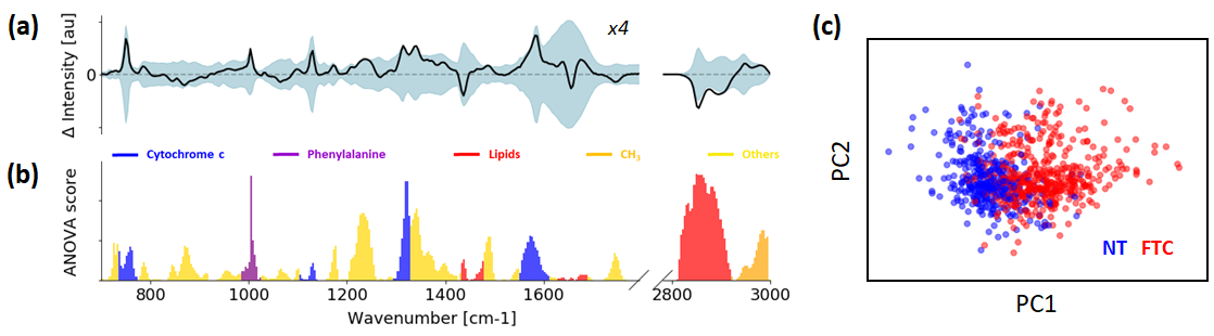
Figure 10: (a) Mean difference spectra of NT vs FTC from cytoplasm regions. (b) ANOVA importance of each wavenumbers, colored according to their main chemical significance to ease the presentation. (c) Each cell spectra is plotted in the PC1 PC2 space colored according to their malignancy, PC1 and PC2 contains together 85% of the explained variance

• FUSE[43] (Multivariate feature selection) evaluates feature subsets by training a predictive model with the selected features and checking how well it performs when making predictions. Because the number of combinations to evaluate scales exponentially with the number of features, it is computationally impractical to try all of the possible combinations and FUSE rely on Monte Carlo Search to look efficiently into the feature set space[44]. This makes possible the detection of the interactions between features and guaranty that the selected feature set is well adapted specifically to our model. Details about FUSE algorithm and score are given in the Methods section. Figure.11a showcases the most important wavenumbers found by FUSE.

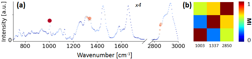
Figure 11: (a) Raman spectra colored as a function of FUSE score (red is high score and blue is low score), top 3 wavenumbers are $1003\text{\,}\mathrm{c}\mathrm{m}^{-1}$ (70%), $1337\text{\,}\mathrm{c}\mathrm{m}^{-1}$ (30%), $2850\text{\,}\mathrm{c}\mathrm{m}^{-1}$ (16%). (b) Mutual information between the top 3 features

To compare the performance of the dimensionality reduction methods described above, we trained a 10-NN and a Random Forest classifier with the obtained set of wavenumbers or principal components. Figure.12 highlight the benefit of FUSE compared to 2 standard dimensionality reduction methods ANOVA and PCA. Classification was performed by taking the first $k$ features ranked after their PC explained variance, ANOVA score and FUSE score, and then training the classifiers with the selected features. The obtained maximal test accuracy of FUSE (averaged over 1000times with bootstrapping) is significantly higher for both random forest and kNN. FUSE maximizes the accuracy at 86% with the 10NN classifier using only two wavenumbers $1003\text{\,}\mathrm{c}\mathrm{m}^{-1}$ and $1337\text{\,}\mathrm{c}\mathrm{m}^{-1}$, for which the peaks can be identified to the proteins phenylalanine and tryptophan. Although cytochrome c and lipids are both informative for the diagnosis of FTC (from ANOVA score), it seems like the combination of the proteins phenylalanine and tryptophan are better indicator for malignancy. Note that an increasing from $84\text{\,}\%$ to $86\text{\,}\%$ represent 16 cells over the 820 initial cells so it can be considered significant. Moreover, the classification did not reveal any particular bad dates where many cells were missclassified, more details about the classification performances are available in supplementary materials.

An interesting tool to further understand the wavenumbers output by FUSE is the mutual information between the selected wavenumbers. In short, it measures the "amount of information" obtained about one variable through another variable. A mutual information of 0 means that the variables are independent, while 1 indicates that they are perfectly correlated, see methods for technical details. The mutual information between $1003\text{\,}\mathrm{c}\mathrm{m}^{-1}$ and $1337\text{\,}\mathrm{c}\mathrm{m}^{-1}$ is 0.5, which is in the middle, it means that they share some information but they can still bring complementary information to each other. On the other hand, $1337\text{\,}\mathrm{c}\mathrm{m}^{-1}$ and $2850\text{\,}\mathrm{c}\mathrm{m}^{-1}$, although representing different chemical species, contains around the same information, meaning that they are strongly correlated to each other.

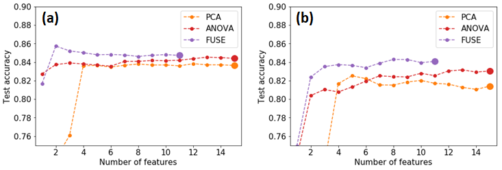
Figure 12: Classification results with (a) 10NN and (b) Random forest after taking the top k features ranked from different dimensionality reduction methods (PCA, ANOVA, FUSE). The test accuracy is averaged over 1000 independent trials with random splitting between test set and training set.

Distribution of the cancer information at the subcellular level

A malignant tissue will not necessarily contain only FTC cells, and on the other hand, our immune system is able to detect and eliminate tiny tumours before they become malignant [45]. As a result, in actual clinical applications, it is unrealistic to assume that all cells in a given tissue would be of the same class. To more accurately reproduce real life clinical application, a mixed culture system that contains both FTC133 and Nthy3-1 cell lines was prepared. After the Raman measurements, discrimination of FTC cells from NT cells was performed by fluorescence measurement (Figure.13a) of the SV40 large T antigen protein, that was previously artificially introduced in Nthy cells for immortalization.

As a final step for our analysis, We investigate how the information about malignancy is spatially distributed in the cells. While we already demonstrated that there is no relevant information for FTC diagnosis in the nucleus, spectral analysis at the pixel level give us information about how the cytoplasm of FTC and NT differs. A cancer index was computed for each pixel in the Raman images using a 10-Nearest neighbor classifier on the 5 first PCs with the training data from our main dataset. A cancer index of 1 indicates a high similarity with FTC cytoplasms and 0 a high similarity with NT cytoplasms. Figure.13b plot the cancer index for a representative image of our mixed culture system. Post classification of the cells was performed by immunostaining (Figure.13a).

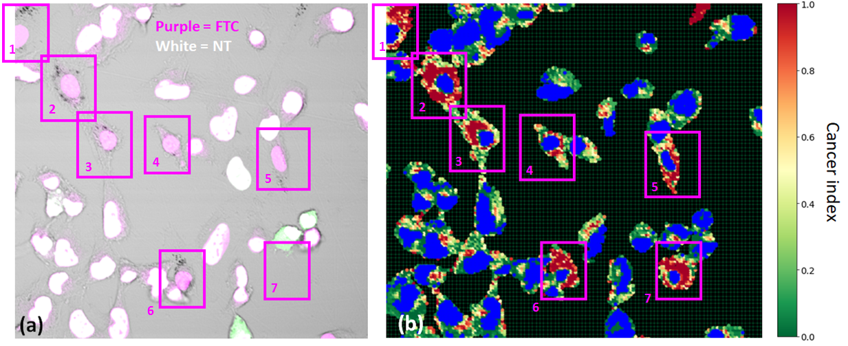
Figure 13: Representative image of the co-culture system (FTC133 and Nthy3-1). (a) Overlay microscopic fluorescence image of SV40 large T protein (magenta) and double strand DNA (green), intensity thresholding was applied for each color. Since Nthy should be positive for both, the color of nuclei in Nthy is white due to the resulting overlay, in contrast, FTC cell is negative for green and positive for magenta, which makes nuclei of FTC cells colored in magenta. White cells surrounded by green regions indicates dividing Nthy. (b) Computed cancer index for each pixel in cytoplasm region, pixels from the background and nucleus regions are colored in black and blue respectively. The cancer cells are framed by a purple rectangle, note that the cell number 7 is missing because it has been washed out during the cleaning process prior to the fluorescence measurement.

We notice that, while FTC cells mainly contain region with a high cancer index in their cytoplasm, NT cells also seems to incorporate some localized high cancer index regions. This indicates the heterogeneity of chemicals within cytoplasm, and the difficulty to find obvious features for malignancy, this is in agreement with previous subcellular analysis of FTC cells [15]. Finding area in the image with high density of red region would allow to automatically detect the presence of FTC cells.

Summary and Discussions

We provided a detailed analysis of hyperspectral Raman images for the diagnosis of Follicular Thyroid Carcinoma and managed to significantly reduce the inconsistencies of Raman measurements over different days by subtracting the mean background spectrum estimated by averaging spectra over non-cell regions in Raman images. We explored various dimensionality reduction methods and emphasized significant importance of lipids, cytochrome c and proteins (Phe, Trp) for the distinction between FTC and NT cell lines. Finally, We also demonstrated that the information for FTC diagnosis is mostly contained in the cytoplasm and not in the nucleus. In conclusion, this systematic analysis of Raman hyperspectral images is an important step toward the increase of the understanding and reliability of Raman measurements for clinical diagnosis.

Future directions    Now that we have better insight about the chemistry involved in the clinical diagnosis of FTC, our procedure should be extended to biological tissues (that differ significantly from cell lines in their chemical composition). One weakness of our analysis is the fact that biological tissues usually involve high cell density which makes the segmentation of cellular structures highly subjective. In addition to that, there is a high biological variance at the single cell level [46]. As a result, classification at the single cell level might not be the most appropriate for clinical diagnosis, and as for further research, one could consider classification of a group of cell rather than single cell to significantly increase the accuracy and reliability [5]. While our study focused on NT and FTC cell lines, one could apply the same analytic procedure to other variants of thyroid lesions or other form of cancers.

Materials and Methods

Sample preparation

Human thyroid follicular carcinoma cell lines (FTC133 and RO82W-1) and human thyroid follicular epitherial cell line (NthyOri3-1) were employed for this research as cancer and non-cancer cells, respectively. The cells were seeded on gelatin-coated dish with a calcium fluoride substrates window (CRYSTRAN LTD, Raman Grade $\text{CaF}_{2}$ CAFP13-0.2). The cell density was $3.0\text{\times}{10}^{5}\text{\,}$ cells/ dish. As for the culturing media, DMEM/Ham’s F-12 (FUJIFILM Wako Pure Chemical Corporation, 61-23201) and RPMI1640 (NACALAITESQUE, INC., 05176-25) were used as basal media for follicular carcinoma cell lines and follicular epitherial cell line, respectively. The basal media were supplemented with 10% fetal bovine serum (FBS) (GE Healthcare, SH3-920.03) and 1% penicillin-streptomycin-L- glutamine solution (FUJIFILM Wako Pure Chemical). The cells were cultured in an incubator at $37\text{\,}\mathrm{\SIUnitSymbolDegree}\mathrm{C}$ with 5% $\text{CO}_{\text{2}}$ and saturated humidity. After 40 to 48 hours incubation, the cells were fixed. The culture media was removed and the cells were washed with $\text{Ca}^{2+}$ and $\text{Mg}^{2+}$+ free phosphate buffered saline (PBS(-)). Then the cells were treated with 4% paraformaldehyde phosphate buffer solution for 10 min. After the treatment, the cells were washed with PBS(-) three times for 5 min each time. Prior to Raman imaging, PBS(-) was filled in culture dish to prevent the drying of the cells.

As for the co-culture system, cancer cell line (FTC133) and non-cancer cell line (NthyOri3-1) were cultured together in the cell density of $0.5\text{\times}{10}^{5}\text{\,}$ cells/ dish each. RPMI1640 supplemented with 10% FBS and 1% penicillin-streptomycin-L-glutamine solution was employed for culture medium. The cell fixation procedure was the same as the one used for independent cell-line culturing.

Data acquisition and Raman Microscopy

Raman imaging of the cells was performed by using line-illumination Raman microscopy [47, 14]. This line-illumination scheme enables the parallel detection of Raman spectra from multiple points in the sample in each exposure, resulting in the acceleration of image acquisition rate, typically 2 order of magnitudes faster than conventional confocal Raman microscope [13]. As a result, the acquisition time of a single Raman image ranged from 20 minutes to 40 minutes in our experiment.

The excitation laser light was shaped into line pattern by a cylindrical lens, then focused on the sample through an objective lens. The Raman scattering induced along the illuminated laser line on the sample was collected with the same objective lens, and then relayed to the slit entrance of a spectrophotometer. On the relaying way, the remaining Rayleigh scattering light was eliminated by longwave-pass edge filters. Raman scattering passing through the entrance slit, which corresponds to the Raman scattering induced by the laser line focus on the sample due to slit-confocal effect, was detected by a cooled CCD camera after being dispersed by a grating inside the spectrophotometer. The output CCD image in a single exposure provided a spectral image, for which the y-axis corresponds to the spatial distribution along the illuminated line and x-axis the spectral frequency (wavenumber). During the imaging process, this CCD exposure was repeated along the direction perpendicular to the line illumination, and the scanning of laser line was manipulated by a galvanometer mirror so that the location of the illuminated laser line on the sample and the entrance slit remained conjugated. The Raman spectral dataset obtained through the imaging process consists of 3-dimensional (x, y, $\lambda$) information as generally-called hyperspectral images.

In this research, the first team used a commercial system (Nanophotn, RAMAN-11) to conduct Raman Microscopy, while the second team performed the measurements with a home-built system. Although both systems adopted a $532\text{\,}\mathrm{n}\mathrm{m}$ CW laser as the excitation light source, the subsequent measurement conditions and installed devices were significantly different in several aspects, as described in the Table.4 below.

Table 4: Experimental setup details of Team 1 and Team 2 (line illumination Raman microscope)

	Team 1 (commercial system)	Team 2 (home-built system)
Excitation light source	$532\text{\,}\mathrm{n}\mathrm{m}$ CW laser	$532\text{\,}\mathrm{n}\mathrm{m}$ CW laser (Coherent, Verdi V18)
Objective lens	60x/1.2, water immersion (Olympus, UPLSAPO 60XW)	40x/NA1.25 (Nikon, CFI Apo 40xWI $\lambda$S)
Edge filter	-	Semrock, LP03-532ER-25
Spectrophotometer	-	Bunkokeiki, MK-300
Grating	$600\text{\,}\mathrm{g}\mathrm{/}\mathrm{m}\mathrm{m}$	$600\text{\,}\mathrm{g}\mathrm{/}\mathrm{m}\mathrm{m}$
Detector	Cooled CCD (Princeton instruments, PIXIS400B eXcelon)	Cooled CCD (Princeton instruments, PIXIS400B eXcelon)
Slit width	$30\text{\,}\mu\mathrm{m}$	$30\text{\,}\mu\mathrm{m}$
Illuminated line width	$32\text{\,}\mu\mathrm{m}$	$25\text{\,}\mu\mathrm{m}$
Pixel resolution on wavenumber axis	$\sim$2.3\text{\,}\mathrm{c}\mathrm{m}^{-1}\mathrm{/}\mathrm{p}\mathrm{i}\mathrm{x}\mathrm{e}\mathrm{l}$$	$\sim$3.2\text{\,}\mathrm{c}\mathrm{m}^{-1}\mathrm{/}\mathrm{p}\mathrm{i}\mathrm{x}\mathrm{e}\mathrm{l}$$
Laser power	$2.7\text{\,}\mathrm{m}\mathrm{W}\mathrm{/}\mu\mathrm{m}^{2}$	$3.3\text{\,}\mathrm{m}\mathrm{W}\mathrm{/}\mu\mathrm{m}^{2}$
Exposure time	$10\text{\,}\mathrm{s}$	$5\text{\,}\mathrm{s}$
Image size	$$122\text{\,}\mu\mathrm{m}$\times(77-107)$\text{\,}\mu\mathrm{m}$$	$$130\text{\,}\mu\mathrm{m}$\times$80\text{\,}\mu\mathrm{m}$$
Sampling	$400\times(250-350)$ pixels	$400\times 240$ pixels

Data calibration

Data calibration consists of assigning the spectral axis of hyperspectral Raman images to their corresponding wavenumber values. An ethanol spectrum was measured prior or posterior to the Raman measurements at each date, and the seven major bands of ethanol (884, 1052, 1096, 1454, 2880, 2930, and $2974\text{\,}\mathrm{c}\mathrm{m}^{-1}$) were used as reference bands for calibration. Generation of the wavenumber axis from original axis was performed by fitting the seven points with a third order polynomial function. Team 1 also performed Raman intensity calibration with halogen lamp as in [48].

Data Preprocessing

Raman data originally contains strong noise, a considerable fluorescence background due to water and glass, as well as cosmic rays, standard preprocessing methods used in our work involve:

• Cosmic rays:
  The spectrum measured at some pixel are altered by cosmic rays, they can be detected when the intensity at a specific wavenumber is at least 8 times the standard deviation higher than the average intensity at that wavenumber: $I(\Delta\omega)\geq 8\sigma(\Delta\omega)+\mu(\Delta\omega)$. Pixel detected with cosmic ray contamination are replaced with the mean of the intensities in the cube surrounding the outlying pixel.

• Noise:
  The intensity of each wave number in the Raman spectrum is following a Poisson distribution, which creates a considerable noise. Denoising is performed by keeping the first 10 components of the measurement matrix $M$ after its Singular Value Decomposition (SVD).

• Fluorescence background:
  All the spectra contain a relatively large background do to glass and water Raman auto-fluorescence, the baseline removal is done with a $7^{\text{th}}$ order recursive polynomial fitting (Polyfit)[28], or by Asymmetric Least Square smoothing (ALS)[29] with parameters $\lambda=$2\text{\times}{10}^{4}\text{\,}$$ and $p=0.05$.

• Normalization:
  While numerous way to normalize are described in literature, the most suitable for our problem is area normalization. Each spectrum is divided by the sum of its intensity over the (700-$1800\text{\,}\mathrm{c}\mathrm{m}^{-1}$) and (2800-$3000\text{\,}\mathrm{c}\mathrm{m}^{-1}$) wavenumber range.

Identification of cellular structure

The differentiation of cell and non cell regions is performed after denoising, ALS background subtraction and normalization. ALS was applied with the coefficients $\lambda=$2\text{\times}{10}^{4}\text{\,}$$ and $p=0.05$.

• Superpixel:
  For the purposes of further increasing the signal-to-noise ratio and reducing the computational cost, adjacent pixels were averaged over spatially-local regions within the images, producing spectra representing groups of pixels, or superpixels. Rather than using a simple binning scheme on a square grid of predetermined size and location, we instead chose the Simple Linear Iterative Clustering (SLIC)[49] pixel clustering method, that is based on spatial proximity and color similarity to better preserve the spatial characteristics of the cells in the Raman images. The number of superpixels per image was chosen such that the superpixels contain an average of 10 individual pixels, which provides superpixels having an average area of $\sim$1\text{\,}\mu\mathrm{m}^{2}$$. The Python implementation from scikit-image library was used.

• Identification of Cells regions:
  The buffer solution used in our measurements is PBS(-) solution, that is characterized by a weak Raman contribution in the high wavenumber region (2800-$3000\text{\,}\mathrm{c}\mathrm{m}^{-1}$). Thus, differentiation of cell regions from non-cell regions is performed by K-means clustering of the intensity averaged over the high wavenumber region: Each spectrum were first partitioned into 8 groups, and the spectra belonging to the 4 most intense clusters were retained as pixels containing cellular regions.

• Identification of non cell regions for background subtraction protocol:
  Defining the 4 less intense clusters as background creates inconsistency over Raman images because it highly depends on the cell density within the image. Thus, to ensure the consistency of background subtraction through different images, non-cell regions are identified by defining a threshold on the high wavenumber region. More precisely, a spectrum is assigned to background if and only if the Raman intensity at $2932\text{\,}\mathrm{c}\mathrm{m}^{-1}$ is within $2\text{\,}\%$ and $10\text{\,}\%$ of the average Raman intensity from cell regions at that wavenumber across all dates.

• Identification of nucleus and cytoplasm regions:
  With an approach similar to the one mentioned above, differentiation of nucleus regions relatively to cytoplasm region is done by K-means clustering on the average intensity of CH2 stretching region ($2842-$2910\text{\,}\mathrm{c}\mathrm{m}^{-1}$$). Each spectrum already associated to cell regions were partitioned into 8 groups, the spectra belonging to the 5 most intense clusters were associated to cytoplasm, and the 3 remaining clusters to nuclei.

• Cell isolation:
  From the binary mask of cell regions, the connected regions of ones, containing cells, were identified with a flood-fill algorithm. Isolated regions containing less than 200 pixels ($<\sim$200\text{\,}\mu\mathrm{m}^{2}$$) are too small to be cells and were discarded. However, because of the relatively high cell density in some Raman images, there is some strong overlap between the cells, and manual segmentation is required to correctly separate the cells.

EMD Distance

The Earth Mover’s Distance (EMD) [34] is a measure of the distance between two probability distributions over a region $D=[d_{i,j}]$. It reflects the minimal amount of work that must be performed to transform one distribution into the other by moving “distribution mass” around. To compute the EMD, we first need to find the optimal flow $F=[f_{i,j}]$ that minimizes the overall cost when moving from P to Q, that can be found by solving a linear optimization problem. The Python library Optimal Transport[35] was used in our work. The EMD is then defined as the minimal work normalized by the total flow:

$$\text{EMD}(P,Q)=\frac{\sum_{i=1}^{n}\sum_{j=1}^{m}f_{i,j}d_{i,j}}{\sum_{i=1}^{n}\sum_{j=1}^{m}f_{i,j}}$$ (1)

Note that the choice of the distance metric $[d_{i,j}]$ will impact the value of EMD. Typically, $[d_{i,j}]$ is taken as euclidean distance, but to ensure consistency of the EMD value over different space, we normalize the distance matrix $[d_{i,j}]$ by the maximum distance between two point in D. Finally, the EMD of two distributions can be generalized to multiple distributions by averaging over the distances of all possible pair of distribution:

$$\text{EMD}(P_{1},..,P_{k})=\frac{1}{k(k-1)}\sum^{k}_{i,j=1}\text{EMD}(P_{i}\ ,\ P_{j})$$ (2)

FUSE

Feature Uct SElection (FUSE)[43] algorithm rely on Monte Carlo tree search to repeatedly evaluate features subset until a candidate for the best feature subset is returned. The feature set space is represented as a Directed Acyclic Graph, and feature subset are evaluated with a kNN classifier. The original FUSE algorithm does not compute a score for each feature but return the best combination of features for a given dataset. We define a score for each features by running FUSE independently 1000 times and increasing the score by 1 if it is in the best feature set, and not otherwise. To avoid overfitting, we run FUSE on 75% of the original dataset and reshuffle the dataset each time. The C++ implementation from [44] was used.

Mutual information

In Shanon’s Information theory, to quantifies the "amount of information" obtained about one random variable $X$ through the other random variable $Y$, one can calculate the Mutual Information (MI) between the two continuous variables, defined as follow:

$$\textit{MI}\hskip 2.0pt(X,Y)=\iint_{X,Y}p(x,y)\log(\frac{p(x,y)}{p(x)p(y)})\,dx\,dy$$

where $p(x,y)$ is the joint probability density function of $X$ and $Y$, and $p(x)$ and $p(y)$ are the marginal probability distribution functions of $X$ and $Y$ respectively. We can also define a normalized version of the mutual information as [50]:

$$I^{*}(X,Y)=\sqrt{1-e^{\hskip 2.0pt-2\times\textit{MI}\hskip 2.0pt(X,Y)}\frac{}{}}$$

$I^{*}=0$ means that $X$ and $Y$ are independent, while $I^{*}=1$ indicates perfectly correlated variables. The mutual information for continuous target variables is estimated with a nonparametric methods based on entropy estimation from $k$-nearest neighbors distances [51] implemented in Python (sklearn library).

References

- [1] He, L., Long, L. R., Antani, S. & Thoma, G. R. Histology image analysis for carcinoma detection and grading. \JournalTitleComputer methods and programs in biomedicine 107, 538–556 (2012).
- [2] Duraiyan, J., Govindarajan, R., Kaliyappan, K. & Palanisamy, M. Applications of immunohistochemistry. \JournalTitleJournal of pharmacy & bioallied sciences 4, S307 (2012).
- [3] Khan, J. et al. Classification and diagnostic prediction of cancers using gene expression profiling and artificial neural networks. \JournalTitleNature medicine 7, 673 (2001).
- [4] Sobrinho-Simoes, M., Eloy, C., Magalhaes, J., Lobo, C. & Amaro, T. Follicular thyroid carcinoma. \JournalTitleModern Pathology 24, S10 (2011).
- [5] Wang, W., Ozolek, J. A. & Rohde, G. K. Detection and classification of thyroid follicular lesions based on nuclear structure from histopathology images. \JournalTitleCytometry Part A: The Journal of the International Society for Advancement of Cytometry 77, 485–494 (2010).
- [6] O’dea, D. et al. Raman spectroscopy for the preoperative diagnosis of thyroid cancer and its subtypes: An in vitro proof-of-concept study. \JournalTitleCytopathology (2018).
- [7] Jegerlehner, S. et al. Overdiagnosis and overtreatment of thyroid cancer: a population-based temporal trend study. \JournalTitlePloS one 12, e0179387 (2017).
- [8] Leboulleux, S., Tuttle, R. M., Pacini, F. & Schlumberger, M. Papillary thyroid microcarcinoma: time to shift from surgery to active surveillance? \JournalTitleThe lancet Diabetes & endocrinology 4, 933–942 (2016).
- [9] Ikeda, H. et al. Raman spectroscopy for the diagnosis of unlabeled and unstained histopathological tissue specimens. \JournalTitleWorld journal of gastrointestinal oncology 10, 439 (2018).
- [10] Santos, I. P. et al. Raman spectroscopy for cancer detection and cancer surgery guidance: translation to the clinics. \JournalTitleAnalyst 142, 3025–3047 (2017).
- [11] Cui, S., Zhang, S. & Yue, S. Raman spectroscopy and imaging for cancer diagnosis. \JournalTitleJournal of Healthcare Engineering 2018 (2018).
- [12] Lui, H., Zhao, J., McLean, D. I. & Zeng, H. Real-time raman spectroscopy for in vivo skin cancer diagnosis. \JournalTitleCancer research canres–4061 (2012).
- [13] Palonpon, A. F. et al. Raman and sers microscopy for molecular imaging of live cells. \JournalTitleNature protocols 8, 677 (2013).
- [14] Hamada, K. et al. Raman microscopy for dynamic molecular imaging of living cells. \JournalTitleJournal of biomedical optics 13, 044027 (2008).
- [15] Taylor, J. N. et al. High-resolution raman microscopic detection of follicular thyroid cancer cells with unsupervised machine learning. \JournalTitleThe Journal of Physical Chemistry B (2019).
- [16] Butler, H. J. et al. Using raman spectroscopy to characterize biological materials. \JournalTitleNature protocols 11, 664 (2016).
- [17] Pence, I. & Mahadevan-Jansen, A. Clinical instrumentation and applications of raman spectroscopy. \JournalTitleChemical Society Reviews 45, 1958–1979 (2016).
- [18] Suen, K. C. Fine-needle aspiration biopsy of the thyroid. \JournalTitleCanadian Medical Association Journal 167, 491–495 (2002).
- [19] Dean, D. S. & Gharib, H. Fine-needle aspiration biopsy of the thyroid gland. \JournalTitleMDText. com, Inc. (2015).
- [20] Cibas, E. S. & Ali, S. Z. The bethesda system for reporting thyroid cytopathology. \JournalTitleAmerican journal of clinical pathology 132, 658–665 (2009).
- [21] Harris, A. T. et al. Raman spectroscopy and advanced mathematical modelling in the discrimination of human thyroid cell lines. \JournalTitleHead & neck oncology 1, 38 (2009).
- [22] Lones, M. A. et al. Discriminating normal and cancerous thyroid cell lines using implicit context representation cartesian genetic programming. In Evolutionary Computation (CEC), 2010 IEEE Congress on, 1–6 (IEEE, 2010).
- [23] Teixeira, C. S. et al. Thyroid tissue analysis through raman spectroscopy. \JournalTitleAnalyst 134, 2361–2370 (2009).
- [24] Rau, J. V. et al. Proof-of-concept raman spectroscopy study aimed to differentiate thyroid follicular patterned lesions. \JournalTitleScientific Reports 7, 14970 (2017).
- [25] Rau, J. V. et al. Raman spectroscopy imaging improves the diagnosis of papillary thyroid carcinoma. \JournalTitleScientific reports 6, 35117 (2016).
- [26] Jha, S. K. & Yadava, R. Denoising by singular value decomposition and its application to electronic nose data processing. \JournalTitleIEEE Sensors Journal 11, 35–44 (2011).
- [27] Jolliffe, I. Principal component analysis. In International encyclopedia of statistical science, 1094–1096 (Springer, 2011).
- [28] Lieber, C. A. & Mahadevan-Jansen, A. Automated method for subtraction of fluorescence from biological raman spectra. \JournalTitleApplied spectroscopy 57, 1363–1367 (2003).
- [29] Eilers, P. H. & Boelens, H. F. Baseline correction with asymmetric least squares smoothing. \JournalTitleLeiden University Medical Centre Report 1, 5 (2005).
- [30] Schie, I. W., Kiselev, R., Krafft, C. & Popp, J. Rapid acquisition of mean raman spectra of eukaryotic cells for a robust single cell classification. \JournalTitleAnalyst 141, 6387–6395 (2016).
- [31] Tenenbaum, J. B., De Silva, V. & Langford, J. C. A global geometric framework for nonlinear dimensionality reduction. \JournalTitlescience 290, 2319–2323 (2000).
- [32] Kochan, K., Peng, H., Wood, B. R. & Haritos, V. S. Single cell assessment of yeast metabolic engineering for enhanced lipid production using raman and afm-ir imaging. \JournalTitleBiotechnology for biofuels 11, 106 (2018).
- [33] Fu, D. & Xie, X. S. Reliable cell segmentation based on spectral phasor analysis of hyperspectral stimulated raman scattering imaging data. \JournalTitleAnalytical chemistry 86, 4115–4119 (2014).
- [34] Rubner, Y., Tomasi, C. & Guibas, L. J. A metric for distributions with applications to image databases. In Sixth International Conference on Computer Vision (IEEE Cat. No. 98CH36271), 59–66 (IEEE, 1998).
- [35] Flamary, R. & Courty, N. Pot python optimal transport library (2017).
- [36] Movasaghi, Z., Rehman, S. & Rehman, I. U. Raman spectroscopy of biological tissues. \JournalTitleApplied Spectroscopy Reviews 42, 493–541 (2007).
- [37] Czamara, K. et al. Raman spectroscopy of lipids: a review. \JournalTitleJournal of Raman Spectroscopy 46, 4–20 (2015).
- [38] Okada, M. et al. Label-free raman observation of cytochrome c dynamics during apoptosis. \JournalTitleProceedings of the National Academy of Sciences 109, 28–32 (2012).
- [39] Rygula, A. et al. Raman spectroscopy of proteins: a review. \JournalTitleJournal of Raman Spectroscopy 44, 1061–1076 (2013).
- [40] De Gelder, J., De Gussem, K., Vandenabeele, P. & Moens, L. Reference database of raman spectra of biological molecules. \JournalTitleJournal of Raman Spectroscopy: An International Journal for Original Work in all Aspects of Raman Spectroscopy, Including Higher Order Processes, and also Brillouin and Rayleigh Scattering 38, 1133–1147 (2007).
- [41] Baenke, F., Peck, B., Miess, H. & Schulze, A. Hooked on fat: the role of lipid synthesis in cancer metabolism and tumour development. \JournalTitleDisease models & mechanisms 6, 1353–1363 (2013).
- [42] Notingher, I., Jell, G., Lohbauer, U., Salih, V. & Hench, L. L. In situ non-invasive spectral discrimination between bone cell phenotypes used in tissue engineering. \JournalTitleJournal of cellular biochemistry 92, 1180–1192 (2004).
- [43] Gaudel, R. & Sebag, M. Feature selection as a one-player game. In International Conference on Machine Learning, 359–366 (2010).
- [44] Pelissier, A., Nakamura, A. & Tabata, K. Feature selection as monte-carlo search in growing single rooted directed acyclic graph by best leaf identification. In Proceedings of the 2019 SIAM International Conference on Data Mining, 450–458 (2019).
- [45] Pandya, P. H., Murray, M. E., Pollok, K. E. & Renbarger, J. L. The immune system in cancer pathogenesis: potential therapeutic approaches. \JournalTitleJournal of immunology research 2016 (2016).
- [46] Kuzmin, A. N., Levchenko, S. M., Pliss, A., Qu, J. & Prasad, P. N. Molecular profiling of single organelles for quantitative analysis of cellular heterogeneity. \JournalTitleScientific reports 7, 6512 (2017).
- [47] Veirs, D. K., Ager, J. W., Loucks, E. T. & Rosenblatt, G. M. Mapping materials properties with raman spectroscopy utilizing a 2-d detector. \JournalTitleApplied optics 29, 4969–4980 (1990).
- [48] Kumamoto, Y. et al. High-throughput cell imaging and classification by narrowband and low-spectral-resolution raman microscopy. \JournalTitleThe Journal of Physical Chemistry B (2019).
- [49] Achanta, R. et al. Slic superpixels compared to state-of-the-art superpixel methods. \JournalTitleIEEE transactions on pattern analysis and machine intelligence 34, 2274–2282 (2012).
- [50] Kojadinovic, I. On the use of mutual information in data analysis: an overview. In Proc Int Symp Appl Stochastic Models Data Anal, 738–47 (2005).
- [51] Kraskov, A., Stögbauer, H. & Grassberger, P. Estimating mutual information. \JournalTitlePhysical review E 69, 066138 (2004).