MxML: Mixture of Meta-Learners
for Few-Shot Classification

Abstract

A meta-model is trained on a distribution of similar tasks such that it learns an algorithm that can quickly adapt to a novel task with only a handful of labeled examples. Most of current meta-learning methods assume that the meta-training set consists of relevant tasks sampled from a single distribution. In practice, however, a new task is often out of the task distribution, yielding a performance degradation. One way to tackle this problem is to construct an ensemble of meta-learners such that each meta-learner is trained on different task distribution. In this paper we present a method for constructing a mixture of meta-learners (MxML), where mixing parameters are determined by the weight prediction network (WPN) optimized to improve the few-shot classification performance. Experiments on various datasets demonstrate that MxML significantly outperforms state-of-the-art meta-learners, or their naïve ensemble in the case of out-of-distribution as well as in-distribution tasks.

1 Introduction

Deep neural networks, trained over a large-scale dataset with legitimate regularization techniques, generalize to a novel instance with persistent performance, while they are highly over-parameterized. Many attempts have been introduced to analyze their generalization performance in notion of sharpness of local minima (Keskar et al., 2017), which describes the reason why deep networks can generalize even if the number of parameters is larger than the number of training instances. Yet, complex deep networks learned from few examples tend to be easily over-fitting to the training set, which is hardly alleviated by a regularization from Bayesian learning (Fei-Fei et al., 2003, 2006; Salakhutdinov et al., 2012).

The primary interest of this paper is few-shot classification: the objective is to learn a mapping function that assigns each instance in a query set $Q$ into few-shot classes defined by a support set $S$, which is composed of a set of few instances in classes. Under this problem setting, meta-learning (Schmidhuber, 1987; Thrun and Pratt, 1998) generalizes to a novel task by learning a series of tasks $\mathcal{E}=\{E_{i}\}_{i=1}^{T}$, where $E_{i}$ is the $i$th episode that consists of a tuple of $Q$ and $S$, and $T$ is the number of training elements. A common practice to train a meta-learner has a major limitation, where tasks in the phase of meta-training and meta-test are sampled from the same dataset. Similar to supervised learning in which training and test distributions are typically matched, meta-learning implicitly assumes that tasks from meta-training and meta-test share similar high-level concepts. Then, the learner performs poorly to a novel task that does not share common attributes of the tasks in meta-training.

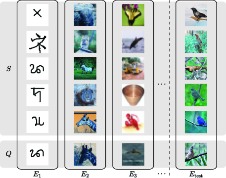
Figure 1: Illustration of solving out-of-distribution task in one-shot scenario. To obtain a model that is capable of learning a task from unseen visual domain, it is necessary to train the model with tasks from diverse distributions with meta-learning. However, naïve training series of episodes $E_{1},E_{2},\ldots$ will degenerate the performance because of distractors.

Rather than learning from a single dataset, we expect meta-learners to be trained over datasets from diverse visual domains, and perform robustly to a novel task by expanding their knowledge from the most similar ones to a novel task. Yet, a naïve training from multiple sets does not perform well because the model considers many irrelevant tasks. To alleviate the effects, an obvious approach is to retrieve similar ones of a novel task and to train a meta-learner from them. This may perform well enough to the target task, but we observe some limitations: (i) learning an appropriate metric between datasets is quite challenging and (ii) a meta-learner is always trained from scratch whenever a new task is given. Instead of selecting similar datasets (Kim et al., 2017), it is better to keep multiple meta-learners trained from each dataset and determine how to aggregate them effectively. This encourages us to build a mixture of meta-learners where mixture coefficients are adaptively determined whenever a novel task is given.

The major concern of building such model is that the model has to determine the coefficient while it glimpses the target task, contrast to the regular supervised learning which has abundant validating examples to evaluate the base learners. To this end, we train the model to learn how to combine the meta-learners given an episode. More specifically, our mixture of meta-learners is established by putting more weight on the base-learner that is expected to perform well to the tasks in the test phase. To evaluate the model given a small number of instances, we employ the weight prediction network (WPN) that predicts the performance of the base learner by observing their latent embeddings of given task. Since WPN determines the performance of the meta-learner based on its output, it can be viewed as a similar idea of meta-recognition system (Scheirer et al., 2012) that analyzes and predicts the recognition system. Hence, learning to evaluate meta-learners can be considered as two layers of meta-learning.

Our contribution is two-fold: (i) we point out a major limitation of the conventional approaches and propose MxML as a solution, such that the mixture coefficients on base meta-learners are task-adaptively determined (ii) we observe that our model achieves the best performance among the state-of-the-art algorithms, when the task is sampled from novel distribution (out-of-distribution) as well as when the task shares the similar attributes with training tasks (in-distribution).

2 Background

This section introduces a problem setting and noticeable works on meta-learning for few-shot classification.

2.1 Problem Setting

We follow the conventional definition of few-shot classification as in (Vinyals et al., 2016; Snell et al., 2017). The objective of few-shot classification is to estimate a function $f({\mathbf{x}};{\boldsymbol{\theta}})$ parameterized by ${\boldsymbol{\theta}}$ that maps an instance of a query set $Q$ into a label set $\mathcal{Y}$. Specifically, the $N$-way $K$-shot classification is formally defined as the task that assigns a query into one of $N$ classes in the support set composed of examples and their associated labels: $S=\{({\mathbf{x}}_{i},y_{i})\}_{i=1}^{NK}$, where an example ${\mathbf{x}}_{i}\in\mathcal{X}$, the associated label $y_{i}\in\mathcal{Y}$, and $|\mathcal{Y}|=N$. Note that the number of examples with the same label is $K$ and $\mathcal{X}$ represents an input space. Similarly, $Q=\{({\mathbf{x}}_{i},y_{i})\}_{i=1}^{L}$, where $L$ is the number of queries and the associated labels are only given in the meta-training.

Meta-learning (Schmidhuber, 1987; Thrun and Pratt, 1998) for few-shot classification introduces an episode, a tuple of $Q$ and $S$ sampled from a dataset, that is used to learn parameters of a model in an episodic training strategy (Vinyals et al., 2016; Snell et al., 2017). It effectively prevents from over-fitting of a model when it is solely trained by a single task. In the subsequent section, we briefly summarize representative meta-learning methods for few-shot classification.

2.2 Related Work

We categorized previous works by the existence of adaptation to few labeled examples of a task in the test phase.

2.2.1 Meta-Learning without Adaptation

Learning appropriate metrics is a key step to solve few-shot learning. Along this direction, matching network (Vinyals et al., 2016) proposes a differentiable nearest neighbor classifier that is learned to minimize the empirical risk computed in the meta-training phase. Given a set of few-shot classes, matching network learns a mapping function from a test instance into one of few-shot classes, which is formulated by bi-directional LSTM with attention mechanism. Prototypical networks (Snell et al., 2017) simply learn a representative vector in each few-shot classes, instead of learning complex neural networks with attention mechanism. This is also trained by a series of episodes, where the prototype vectors are learned to enforce that they should be close in the same class. Moreover, its simple extension to learn covariance structures is also available at (Fort, 2017). Among early works on this direction, Siamese neural network (Koch et al., 2015) is used to learn the metric that preserves semantic similarities between instances.

2.2.2 Meta-Learning with Adaptation

Learning models that quickly adapt to few examples is critical to solve few-shot learning. Along this direction, model-agnostic meta-learning (MAML) explicitly trains a meta-learner such that few updates with labeled instances are enough to achieve high generalization performance on a new task (Finn et al., 2017). The original implementation of MAML requires a second-order derivative of parameters of deep neural network, which is accelerated by a first-order approximation (Nichol et al., 2018). Similarly, Ravi and Larochelle (2017) propose a meta-learning framework such that LSTM is trained to learn an update rule for few-shot learning. To further advance this direction, Lee and Choi (2018) explicitly split a meta-learner into task-specific and task-general components, where each component is updated in a more effective way, compared to update them simultaneously.

2.2.3 Set-Input Network 

Neural networks that are capable of being invariant to permutation and dealing with variable-length inputs have recently gained a lot of attention to learn semantic representation of sets. Zaheer et al. (2017) provide a theoretical justification to a unique structure of neural networks that is invariant to permutation, which is able to being deployed to many interesting applications: multiple instance learning, point-cloud classification, etc. Edwards and Storkey (2017) develop a generative process of a set given a context vector, which is inferred by a statistic network that takes into account the exchangeability of a dataset. Moreover, Lee et al. (2018) propose a feed-forward neural network with self-attention, which still holds permutation-invariant property.

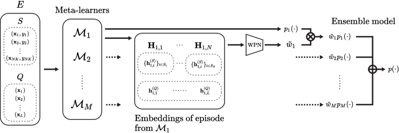
Figure 2: Architecture of MxML that produces a class probability of the ensemble model. The mixture coefficient for the base meta-learners are determined by embedding vectors of episode from each meta-learner. The inputs of network are a query set $Q$ and a support set $S$. $m$th meta-learner generates ${\mathbf{H}}_{m,1},\ldots,{\mathbf{H}}_{m,N}$ and ${\mathbf{h}}_{m,1}^{(Q)},\ldots,{\mathbf{h}}_{m,L}^{(Q)}$, and the output of MxML is produced by the linear combination of class probabilities of meta-learners with the weights from WPN.

3 Main Algorithm

In this section, we introduce our main algorithm to train mixture of meta-learners in a task-adaptive fashion.

3.1 Mixture of Meta-Learners (MxML)

Mixture of meta-learners (MxML) task-adaptively aggregates base meta-learners, in which mixture coefficients are determined by weight prediction network (WPN). Figure 2 introduces an overall structure of MxML that generates $M$ representations of an episode to determine the weight proportion of meta-learners by WPN. Specifically, an episode composed of $(S,Q)$ is transformed by the $m$th base meta-learner as follows:

$$\left({\mathbf{h}}_{m}^{(S)},{\mathbf{h}}_{m}^{(Q)}\right)\coloneqq\left(\{{\mathbf{h}}^{(S)}_{m,i}\}_{i=1}^{NK},\{{\mathbf{h}}_{m,i}^{(Q)}\}_{i=1}^{L}\right),$$ (1)

where ${\mathbf{h}}^{(S)}_{m,i}$, ${\mathbf{h}}_{m,i}^{(Q)}$ are the hidden representations of the $i$th instance in the support and query set, respectively. To ease exploiting the label information, we collect $K$ instances that belong to the same label and denote the hidden representations of them as ${\mathbf{H}}_{m,n}=\{{\mathbf{h}}_{m,j}^{(S)}\}_{j\in S_{n}}$, where $S_{n}$ means the subset of support set that only contains the data labeled as $n$. Hence, we denote ${\mathbf{H}}_{m}=\{{\mathbf{H}}_{m,n}\}_{n=1}^{N}$.

Then, the final prediction of MxML is established by combining the predictions of meta-learners with mixing coefficients as follows:

$$p({\mathbf{x}}|S;{\boldsymbol{\theta}},{\boldsymbol{\psi}})=\sigma\left(\sum_{m=1}^{M}w\left({\mathbf{H}}_{m},{\mathbf{h}}_{m}^{(Q)};{\boldsymbol{\theta}}\right)p_{m}({\mathbf{x}}|S;{\boldsymbol{\psi}})\right),$$ (2)

where $w({\mathbf{H}}_{m},{\mathbf{h}}_{m}^{(Q)};{\boldsymbol{\theta}})$ means the importance of each meta-learner from WPN parameterized by ${\boldsymbol{\theta}}$, $p_{m}({\mathbf{x}}|S;{\boldsymbol{\psi}})$ represents the prediction of ${\mathbf{x}}\in Q$ by the $m$th base meta-learner, and $\sigma(\cdot)$ is a softmax function. Details on WPN are described in the subsequent section.

MxML requires a two-step training procedure for base learners and WPN, in which $M$ datasets are given. For the first step, each meta-learner is trained from its associated dataset, and fixed throughout the next step. MxML allows us to choose any type of meta-learners including prototypical network (Snell et al., 2017) and MAML (Finn et al., 2017). For the second step, WPN is trained by a series of episodes sampled from $M$ diverse datasets. In this step, ${\boldsymbol{\theta}}$ is trained by minimizing the cross-entropy between weighted prediction (2) and the associated labels, while ${\boldsymbol{\psi}}$ is fixed after training base meta-learners. The objective function is introduced as follows:

$$\operatornamewithlimits{\arg\max}_{{\boldsymbol{\theta}}}\mathbb{E}_{R\sim D}\left[\mathbb{E}_{(S,Q)\sim R}\left[\frac{1}{L}\sum_{({\mathbf{x}},y)\in Q}y\log p({\mathbf{x}}|S;{\boldsymbol{\theta}},{\boldsymbol{\psi}})\right]\right],$$ (3)

where $D$ refers to a dataset distribution which is defined in the space that all of the datasets exists, $R$ means a single dataset sampled from $D$, and $E$ represents an episode from selected dataset $D$.

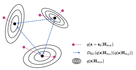
Figure 3: Visualization of components for weight prediction of $m$th meta-learner. $q({\mathbf{z}}|{\mathbf{H}}_{m,n})$ is a distribution of $n$th class in the support set (blue circles), $q({\mathbf{z}}_{k}|{\mathbf{H}}_{m,n})$ is a probability density of a query from the most closest distribution (red dot), and the KL divergences are denoted as green arrows. Predicted weight for the base meta-learner is large if the sum of KL divergences is large (classes are separable), and product of the log density of query predictions is large (queries are correctly predicted with high confidence).

3.2 Weight Prediction Network (WPN)

To measure the importance of $m$th learner, WPN introduces a distribution that encodes ${\mathbf{H}}_{m,n}$ into a vector, denoted as $q({\mathbf{z}}|{\mathbf{H}}_{m,n};{\boldsymbol{\theta}})$, which is parameterized by ${\boldsymbol{\theta}}$. We expect that the base meta-learner performs reasonably well when the inter-class distributions are separable and the predicted class of a query is highly concentrated on a specific class. In this sense, the weight prediction on $m$th learner is defined as follows:

$$w\left({\mathbf{H}}_{m},{\mathbf{h}}_{m}^{(Q)};{\boldsymbol{\theta}}\right) =\frac{1}{N^{2}}\sum_{i,j=1}^{N}D_{\textrm{KL}}\left(q({\mathbf{z}}|{\mathbf{H}}_{m,i};{\boldsymbol{\theta}})\|q({\mathbf{z}}|{\mathbf{H}}_{m,j};{\boldsymbol{\theta}})\right)$$

$$\quad+\lambda\sum_{k=1}^{L}\log\left(S\left(\left\{q\left({\mathbf{z}}={\mathbf{z}}_{k}|{\mathbf{H}}_{m,n};{\boldsymbol{\theta}}\right)\right\}_{n=1}^{N}\right)\right)$$ (4)

where $q({\mathbf{z}}|{\mathbf{H}}_{m,n})$ is a distribution over the latent vectors that belong to $n$th class in the support set (referred to as class-specific distribution), ${\mathbf{z}}_{k}$ refers the latent vector of $k$th query, and $S(\cdot)$ is the smooth max function that returns the maximum component in the set in a differentiable way. We assume that $q({\mathbf{z}}|\cdot)$ is a multivariate normal distribution with zero off-diagonal entries. Mean and diagonal variances of $q({\mathbf{z}}|{\mathbf{H}}_{m,i})$ are given from the neural network with input ${\mathbf{H}}_{m,i}$. Since ${\mathbf{H}}_{m,i}$ is a set of embeddings, set encoding network is needed. Bi-directional LSTM is used in (Vinyals et al., 2016) and average pooling-based set representation method is used in (Zaheer et al., 2017; Edwards and Storkey, 2017). Likewise, we also use average vectors for encoding ${\mathbf{H}}_{m,i}$ because of its simplicity. Exact implementation details are shown in Table 2.

The first part of the right-hand side of (4) explains the distance between class-specific distributions. We assume that the value of the term will increase when the classes in the task are more separable than other meta-learners. In the second part of (4), ${\mathbf{z}}_{k}$ is obtained from the neural network with input ${\mathbf{h}}_{k}^{(S)}$. The probability density in the point ${\mathbf{z}}_{k}$ from the nearest distribution is multiplied over the entire query. Apparently, this term is cumulative, so utilizing more number of queries make $w(\cdot,\cdot;{\boldsymbol{\theta}})$ more dependent on the second part. Figure 3 shows graphical visualization of each component.

WPN is trained by optimizing the parameters thereof from minimizing the cross entropy loss between prediction of MxML and the true label (see Algorithm 1). This formulation explicitly consider training WPN from diverse datasets to generalize on the novel one.

Our insight to use the parameterized WPN and train them to predict the model performance is because the evaluation for the model from (4) is not a perfect metric. Actually, it is not easy to validate the model without any similar instances from the target. Since the target task is given as an episode, we can barely estimate based on the task embedding structure. By building a structured weight inference instead of using the model that inputs a set of embedding vectors and outputs a single weight prediction, it keeps from over-fitting to a simple selection of single meta-learner.

Algorithm 1 Optimization of WPN

0:  Base meta-learners learned from each dataset $\{p_{m}(\cdot)\}_{m=1}^{M}$ and multiple datasets $\{D_{g}\}_{g=1}^{G}$.

0:  Learned parameters ${\boldsymbol{\theta}}$.

1:  Initialize ${\boldsymbol{\theta}}$ randomly.

2:  while not done do

3:     Select $R$ from $\{D_{g}\}_{g=1}^{G}$ randomly.

4:     Sample an episode $E\sim R$, where ${E=(S,Q)}$.

5:     for $i=1,2,\ldots,M$ do

6:        Determine $w_{i}$ by (4)

7:     end for

8:     Compute $p({\mathbf{x}})$ with $\{w_{j}\}_{j=1}^{M}$ in (2).

9:     Optimize WPN parameterized by ${\boldsymbol{\theta}}$ by minimizing (3).

10:  end while

3.3 Discussion

In order to handle a novel few-shot learning task, the model needs to be trained over similar set of tasks. But in case that there is no available similar set of tasks, or more specifically, if there is no other training classes containing plenty amount of instances in the same visual domain with the target, then the model should be trained from diverse domain to generalize to a novel one. We mainly focus on this problem setting which we consider more realistic.

In the ensemble methods in classical supervised learning, the base learners should be accurate as possible. They are evaluated with validating examples which has the same distributional property with the test examples, and only good ones of them are used to combine (otherwise, the model degenerates). It is also similar in meta-learning phase if we assume that the target tasks are achieved from known domain and similar (but not exact) tasks can be collected so that we can validate the models, then we can possibly attain good ones.

In case of the target task is given from the first seen distribution, however, then there are no available validating examples for the base meta-learners since it contains only few-shot training examples ($S$) with some test instances ($Q$). Our main proposal is to build a model that evaluates the meta-learner given an episode to select the best performing model depending on distributional property of the task so that the model can be capable of solving any kind of tasks. Since the episode is composed of two sets $(S,Q)$, we formulate this as a set-based problem. Sometimes $S$ contains too small instances to evaluate the model, we found that utilizing query instances helps a lot (i.e., transductive setting).

Table 1: Description of datasets used in meta-training and -test, which includes the number of images $N_{\textrm{img}}$, the number of total classes $N_{\textrm{cls}}$, the number of classes used for training meta-learners and WPN, and the average image size of each dataset. Our experiment protocol requires splitting classes of each dataset in meta-training into two exclusive sets: one is used for training base-learners and the other is for training WPN.

Type	Dataset	$N_{\textrm{img}}$	$N_{\textrm{cls}}$	Split	Average of (H, W)
Meta-train	CIFAR-100	60,000	100	(80/20)	(32, 32)
	VOC2012	11,540	20	(20/-)	(386, 470)
	AwA2	37,322	50	(40/10)	(713, 908)
	Caltech256	30,607	256	(205/51)	(325, 371)
	Omniglot	32,460	1,623	(1,298/325)	(105, 105)
Meta-test	MNIST	70,000	10	(-/-)	(28, 28)
	CIFAR-10	60,000	10	(-/-)	(32, 32)
	CUB200	11,788	200	(-/-)	(386, 467)
	Caltech101	9,146	101	(-/-)	(244, 301)
	miniImageNet	60,000	100	(-/-)	(469, 387)

Table 2: Details of implementation including input/output and layers of components of MxML for $m$th meta-learner and WPN. ConvBlock is composed of series of convolutional layer, batch normalization, and ReLU activation function. Each convolutional layer contains the kernel with size (3,3) and the channel with 64 for protoypical network and 32 for MAML, as implemented originally. Avg refers the mean vector of all instances in ${\mathbf{H}}_{m,n}$ (see equation 1) which is fed to dense layer to produce ${\boldsymbol{\mu}}_{m,n},{\boldsymbol{\sigma}}_{m,n}\in\mathbb{R}^{d_{z}}$, means and log diagonal variances of class-specific distribution.

	Meta-learner	WPN
Input	$(S,Q)$	${\mathbf{H}}_{m}$	${\mathbf{h}}_{m}^{(Q)}$
Layer	4 ConvBlocks	Avg, $\textrm{Dense}(2d_{z})$	$\textrm{Dense}(d_{z})$
		$\xrightarrow{}\{({\boldsymbol{\mu}}_{m,n},\log{\boldsymbol{\sigma}}_{m,n}^{2})\}_{n=1}^{N}$	$\xrightarrow{}\{{\mathbf{z}}_{k}\}_{k=1}^{L}$
Output	$({\mathbf{H}}_{m},{\mathbf{h}}_{m}^{(Q)})$	$w_{m}$

4 Experiments

In this section, we show that our methods outperform other existing methods. First, we introduce the datasets used in this paper and the detailed settings of the experiments.

4.1 Datasets

We use various image datasets to train and test our network. Five datasets are used to train base meta-learners and WPN, and distinct five datasets are used for the phase of meta-test. For the fair comparison, we collect datasets in a basis of four categories:

• Gray-scale low/high resolution images. We use Omniglot (Lake et al., 2015) and MNIST (LeCun and Cortes, 1998) in this category. Omiglot is used for training base-learners and MxML and MNIST is used for the meta-test phase, because the number of classes is not large enough for training meta-learners.

• Colored low-resolution images. We use CIFAR-10 and CIFAR-100 (Krizhevsky, 2009), where the former is used for the meta-test phase and the latter is used for training meta-learners.

• Colored high-resolution animal images. We employ AwA2 (Xian et al., 2017) and CUB200 (Welinder et al., 2010): the former consists of high-resolution animal images crawled from web sites and the latter is composed of images from 50 species of birds. CUB200 is originally designed for fine-grained classification, then this is relatively difficult to achieve the high performance.

• Colored high-resolution generic object images. We use VOC2012 (Everingham et al., 2010), miniImageNet (Fei-Fei et al., 2004), and Caltech101/Caltech256 (Griffin et al., 2007) in this category. All of them consist of high-resolution images of generic objects.

Table 1 summarizes statistics and experiment settings of each dataset: which dataset is used for the phase of meta-training or meta-test, and the number of classes used for training meta-learners and WPN. We simply remark that all datasets are pre-processed in the same fashion, where images are resized into $84\times 84$ resolution and gray-scale images are converted into 3-channel images.

4.2 Experimental Details

We set parameters of WPN as $d_{z}=128$, $\lambda=10^{-1}$, with fixed learning rate $10^{-4}$ using Adam optimizer (Kingma and Ba, 2015). While training and testing, 15 queries with single meta-batch is given. The parameters of prototypical network is set similar to original setting except for the learning rate that starts from $10^{-3}$ and decreases to $10^{-4}$ when it approaches 70 epoch out of 100 epochs. We use second order MAML with inner loop learning rate $3\times 10^{-2}$, and the same learning rate used in prototypical network. While training, meta-batch size is fixed to 2 in the entire out-of-distribution task and 1-shot in-distribution task, and 4 in 5-shot in-distribution task.

In addition, we empirically observe that normalized features are effective to train WPN. Thus, in this paper all of the features extracted from base meta-learners are normalized as:

$${\mathbf{\hat{h}}}_{p}=\frac{{\mathbf{h}}_{p}}{\|{\mathbf{h}}_{p}\|_{2}}\quad\textrm{and}\quad{\mathbf{\hat{h}}}_{q}=\frac{{\mathbf{h}}_{q}}{\|{\mathbf{h}}_{q}\|_{2}},$$ (5)

where ${\mathbf{h}}_{p}\in\mathbb{R}^{d}$ and ${\mathbf{h}}_{q}\in\mathbb{R}^{d}$ are $d$-dimensional representation of support and query vectors, respectively. We assume that the normalization helps to standardize a scale in embedding spaces learned from different datasets.

Table 3: 10-way 5-shot classification results of MxML with prototypical networks as base meta-learners and baselines. Transductive and non-transductive setting are denoted as Trans./Non-trans., respectively. CUB and mImgNet indicate CUB200 and miniImageNet. The results are obtained from average accuracy of 600 episodes with query size 15.

Model	Meta-train	Meta-test
		MNIST	CUB	CIFAR-10	Caltech101	mImgNet
Dataset-specific model	AwA2	75.21	38.14	27.22	55.96	32.02
	CIFAR-100	77.63	29.83	45.87	61.19	35.38
	Omniglot	73.13	17.12	17.25	29.46	21.06
	VOC2012	67.24	24.72	24.42	46.65	28.71
	Caltech256	79.48	39.08	33.73	78.13	43.80
Single model	Multiple datasets	76.72	39.20	39.34	75.05	44.66
Uniform averaging		80.04	41.38	39.46	73.88	45.10
MxML (Non-trans.)		80.25	42.62	43.92	77.32	46.34
MxML (Trans.)		80.42	43.13	46.17	78.55	46.62

Table 4: 10-way 5-shot classification results of MxML with MAML as base meta-learners and baselines. It follows same settings in Table 4.2.

Model	Meta-train	Meta-test
		MNIST	CUB	CIFAR-10	Caltech101	mImgNet
Dataset-specific model	AwA2	50.98	37.13	19.71	46.44	31.80
	CIFAR-100	60.73	32.82	39.27	56.51	39.76
	Omniglot	68.51	18.00	19.62	29.69	21.64
	VOC2012	48.24	22.67	19.91	38.58	28.09
	Caltech256	56.56	38.49	29.69	67.27	41.16
Single model	Multiple datasets	58.62	39.25	35.97	63.75	43.83
Uniform averaging		72.73	39.28	32.66	65.57	43.33
MxML (Non-trans.)		72.26	42.02	36.24	65.91	43.28
MxML (Trans.)		72.53	43.73	39.42	67.66	45.73

4.3 Out-of-distribution

We design out-of-distribution task to verify that our model performs robustly on the few-shot classification task sampled from first seen distribution. We use 5 datasets to train the model (i.e., AwA2, CIFAR-100, Omniglot, VOC2012, and Caltech256), and evaluate it from 5 separate datasets (i.e., MNIST, CUB-200, CIFAR-10, Caltech101, and miniImageNet). The classes of each meta-train dataset are randomly split into 2 subsets. One (80% of entire classes) is used to train class-specific meta-learners, and the other (20% of entire classes) is used to train WPN that learns from diverse task distribution.

The results of the experiments are shown in Table 4.2 (with base meta-learner as prototypical network) and Table 4.2 (with base meta-learner as MAML). Dataset-specific models are only trained within their associated dataset, and their classification results for each meta-test datasets are listed. When some datasets share the common source (i.e., the same visual domain so they have the similar image resolution) or share the similar tasks (classifying among animals, or general objects) then the class-specific models tend to perform well on the target dataset. However, that is not always true on some cases such as Omniglot to MNIST. We can expect that the model trained on Omniglot performs the most on MNIST dataset because both of them consider gray-scale character images, but Caltech256 trained meta-learner is the stronger classifier. This is a supporting reason to building MxML rather than using a similar dataset manually because it is difficult to notice that model would perform the best in advance.

Single model has an identical structure with a dataset-specific model, but is trained on multiple datasets. In many cases, we observe that the performance degrades than well-performing single learner because of many irrelevant tasks from unrelated domains. Uniform averaging model is a mixture model of dataset-specific models with identical mixture coefficient. Also in this case, some models are degrading.

Figure 4 shows the averages and standard deviations of mixing coefficient on base learners associated with datasets, when CUB200 or CIFAR10 is given as a meta-test dataset. When there exists a relevant dataset to the target task, MxML assigns relatively high coefficient to the dataset. We observe that the weight on the base learner from CIFAR100 is much higher than the ones from other datasets when the tasks are given from CIFAR10. On the contrary, MxML assigns large coefficient on AwA2 and Caltech256 when the tasks are generated from CUB200, where all of them contain the tasks of classifying animals.

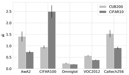
Figure 4: Mixture coefficients (as vertical axis) on base meta-learners trained from the associated datasets (as horizontal axis) for 10-way 5-shot MxML (Trans.). The mean and standard deviation of ensemble weights are computed by 600 episodes from meta-test set.

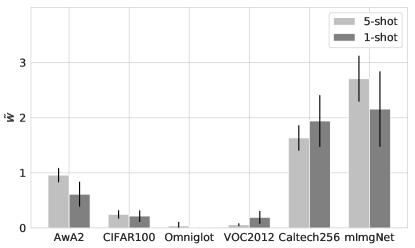
Figure 5: Mixture coefficients (as vertical axis) on base meta-learners trained from the associated dataset (as horizontal axis), in case of 5-way few-shot classification task from miniImageNet.

4.4 In-distribution

In in-distribution task, we show that our model performs good as well when the task is sampled from the already-seen distribution. We make slight change from the out-of-distribution experiment setting. From the setting in Table 1, miniImageNet (denoted as mImgNet) dataset is split into 3 subsets as in  Vinyals et al. (2016) with the number of classes 64/16/20 (meta-train/validation/test). One base meta-learner trained on miniImageNet dataset is added compare to the previous setting, and is tested only on the miniImageNet dataset. The result shows that our model consistently improves the performance in the conventional $N$-way $K$-shot classification problem with additional meta-learners trained on other datasets (Table 5). Figure 5 shows the mixing coefficients of base meta-learners, in which MxML puts more attentions on miniImageNet and Caltech256 in both 1-shot and 5-shot experiments.

Table 5: Accuracy with 95% confidence interval of MxML with prototypical network as a base meta-learners in 5-way classification task sampled from miniImageNet of which non-overlapping classes are included in the meta-training.

Model	1-shot	5-shot
Dataset-specific model	50.741 (0.764)	67.781 (0.664)
Single model	47.432 (0.750)	65.729 (0.641)
Uniform Averaging	44.618 (0.756)	66.007 (0.667)
MxML	51.393 (0.765)	69.338 (0.642)

5 Conclusion

In this paper, we propose a task-adaptive mixture of meta-learners, referred to as MxML for few-shot classification. We observe that a common practice for meta-learning has a major limitation: tasks used in the meta-training and meta-test phases are sampled from the similar task distribution. To resolve this critical issue, we tackle a challenging problem in which a test task is sampled from a novel dataset. We then propose an ensemble network that learns how to adaptively aggregate base meta-learners for the given task. Extensive experiments on diverse datasets confirm that MxML outperforms other baselines.

References

- Edwards and Storkey [2017] H. Edwards and A. Storkey. Towards a neural statistician. In Proceedings of the International Conference on Learning Representations (ICLR), 2017.
- Everingham et al. [2010] M. Everingham, L. Van Gool, C. K. I. Williams, J. Winn, and A. Zisserman. The Pascal visual object classes (VOC) challenge. International Journal of Computer Vision, 2010.
- Fei-Fei et al. [2003] L. Fei-Fei, R. Fergus, and P. Perona. A bayesian approach to unsupervised one-shot learning of object categories. In Proceedings of the International Conference on Computer Vision (ICCV), 2003.
- Fei-Fei et al. [2004] L. Fei-Fei, R. Fergus, and P. Perona. Learning generative visual models from few training examples: an incremental Bayesian approach tested on 101 object categories. Computer Vision and Image Understanding, 2004.
- Fei-Fei et al. [2006] L. Fei-Fei, R. Fergus, and P. Perona. One-shot learning of object categories. IEEE Transactions on Pattern Analysis and Machine Intelligence, 2006.
- Finn et al. [2017] C. Finn, P. Abbeel, and S. Levine. Model-agnostic meta-learning for fast adaptation of deep networks. In Proceedings of the International Conference on Machine Learning (ICML), 2017.
- Fort [2017] S. Fort. Gaussian prototypical networks for few-shot learning on omniglot. arXiv e-prints, arXiv:1708.02735, 2017.
- Griffin et al. [2007] G. Griffin, A. Holub, and P. Perona. Caltech-256 object category dataset. Technical report, California Institute of Technology, 2007.
- Keskar et al. [2017] N. S. Keskar, D. Mudigere, J. Nocedal, M. Smelyanskiy, and P. T. P. Tang. On large-batch training for deep learning: Generalization gap and sharp minima. In Proceedings of the International Conference on Learning Representations (ICLR), 2017.
- Kim et al. [2017] J. Kim, S. Kim, and S. Choi. Learning to warm-start Bayesian hyperparameter optimization. arXiv e-prints, arXiv:1710.06219, 2017.
- Kingma and Ba [2015] D. K. Kingma and J. Ba. Adam: A method for stochastic optimization. In Proceedings of the International Conference on Learning Representations (ICLR), 2015.
- Koch et al. [2015] G. Koch, R. Zemel, and R. Salakhutdinov. Siamese neural networks for one-shot image recognition. In Proceedings of the International Conference on Machine Learning (ICML), 2015.
- Krizhevsky [2009] A. Krizhevsky. Learning multiple layers of features from tiny images. Technical report, University of Toronto, 2009.
- Lake et al. [2015] B. M. Lake, R. Salakhutdinov, and J. B. Tenenbaum. Human-level concept learning through probabilistic program induction. Science, 2015.
- LeCun and Cortes [1998] Y. LeCun and C. Cortes. The MNIST database of handwritten digits, 1998. http://yann.lecun.com/exdb/mnist/.
- Lee et al. [2018] J. Lee, Y. Lee, J. Kim, A. R. Kosiorek, S. Choi, and Y. W. Teh. Set transformer: A framework for attention-based permutation-invariant neural networks. arXiv e-prints, arXiv:1810.00825, 2018.
- Lee and Choi [2018] Y. Lee and S. Choi. Gradient-based meta-learning with learned layerwise metric and subspace. In Proceedings of the International Conference on Machine Learning (ICML), 2018.
- Nichol et al. [2018] A. Nichol, J. Achiam, and J. Schulman. On first-order meta-learning algorithms. arXiv e-prints, arXiv:1803.02999, 2018.
- Ravi and Larochelle [2017] S. Ravi and H. Larochelle. Optimization as a model for few-shot learning. In Proceedings of the International Conference on Learning Representations (ICLR), 2017.
- Salakhutdinov et al. [2012] R. Salakhutdinov, J. Tenenbaum, and A. Torralba. One-shot learning with a hierarchical nonparametric bayesian model. In Proceedings of ICML Workshop on Unsupervised and Transfer Learning, 2012.
- Scheirer et al. [2012] W. J. Scheirer, A. Rocha, R. J. Micheals, and T. E. Boult. Meta-recognition: The theory and practice of recognition score analysis. IEEE Transactions on Pattern Analysis and Machine Intelligence, 2012.
- Schmidhuber [1987] J. Schmidhuber. Evolutionary Principles in Self-Referential Learning. PhD thesis, Technical University of Munich, 1987.
- Snell et al. [2017] J. Snell, K. Swersky, and R. S. Zemel. Prototypical networks for few-shot learning. In Advances in Neural Information Processing Systems (NeurIPS), 2017.
- Thrun and Pratt [1998] S. Thrun and L. Pratt. Learning to learn. Kluwer Academic Publishers Norwell, 1998.
- Vinyals et al. [2016] O. Vinyals, C. Blundell, T. P. Lillicrap, K. Kavukcuoglu, and D. Wierstra. Matching networks for one shot learning. In Advances in Neural Information Processing Systems (NeurIPS), 2016.
- Welinder et al. [2010] P. Welinder, S. Branson, T. Mita, C. Wah, F. Schroff, S. Belongie, and P. Perona. Caltech-UCSD Birds 200. Technical report, California Institute of Technology, 2010.
- Xian et al. [2017] Y. Xian, C. Lampert, B. Schiele, and Z. Akata. Zero-shot learning - A comprehensive evaluation of the good, the bad and the ugly. IEEE Transactions on Pattern Analysis and Machine Intelligence, 2017.
- Zaheer et al. [2017] M. Zaheer, S. Kottur, S. Ravanbakhsh, B. Poczos, R. R. Salakhutdinov, and A. J. Smola. Deep sets. In Advances in Neural Information Processing Systems (NeurIPS), 2017.