On the Polarized Nonthermal Emission from AR Scorpii

Abstract

We study linear polarization of optical emission from white dwarf (WD) binary system AR Scorpii. The optical emission from this binary is modulating with the beat frequency of the system, and it is highly polarized, with the degree of the polarization reaching $\sim 40$%. The angle of the polarization monotonically increases with the spin phase, and the total swing angle can reach $360^{\circ}$ over one spin phase. It is also observed that the morphology of the pulse profile and the degree of linear polarization evolve with the orbital phase. These polarization properties can constrain the scenario for nonthermal emission from AR Scorpii. In this paper, we study the polarization properties predicted by the emission model, in which (i) the pulsed optical emission is produced by the synchrotron emission from relativistic electrons trapped by magnetic field lines of the WD and (ii) the emission is mainly produced at magnetic mirror points of the electron motion. We find that this model can reproduce the large swing of the polarization angle, provided that the distribution of the initial pitch angle of the electrons that are leaving the M-type star is biased to a smaller angle rather than a uniform distribution. The observed direction of the swing suggests that the Earth viewing angle is less than $90^{\circ}$ measured from the WD spin axis. The current model prefers an Earth viewing angle of $50^{\circ}-60^{\circ}$ and a magnetic inclination angle of $50^{\circ}-60^{\circ}$ (or $120^{\circ}-130^{\circ}$). We discuss that the different contribution of the emission from M-type star to total emission causes a large variation in the pulsed fraction and the degree of the linear polarization along the orbital phase.

1. Introduction

AR Scorpii (hereafter AR Sco) is a binary system composed of a white dwarf (WD) and an M-type main-sequence star, which has a radius of $R_{*}\sim 0.3R_{\odot}$ and a mass of $M_{*}\sim 0.3M_{\odot}$ (Marsh et al. 2016; Buckley et al. 2017). The WD of AR Sco shows fast spinning with a period of $P_{WD}\sim 117$s and an orbital period of $P_{orb}\sim 3.65$hr. The distance to the system from Earth is estimated to be $d\sim 110$pc. AR Sco is the first WD that shows a radio emission modulating with the spin period of the WD. Marsh et al. (2016) measure a spin-down rate of the WD of $\dot{f}\sim-2.86\times 10^{-17}{\rm Hz~{}s^{-1}}$ and estimate $B_{s}\sim 10^{8}$G for the surface magnetic field of the WD. Potter & Buckley (2018a), on the other hand, report that new optical data are inconsistent with the published spin-down rate but consistent with a constant spin period. Later, Stiller et al. (2018) measure a spin-down rate of $\dot{f}\sim-5.14\times 10^{-17}{\rm Hz~{}s^{-1}}$. Although more observation would be required to determine the spin down rate, the suggested values indicate that the radiation from AR Sco is powered by dissipation of the high magnetic field ($>10^{8}$G) of the WD. AR Sco could eventually evolve to a ’polar’, for which a sufficiently large magnetic field locks the two stars into synchronous rotation with an orbital period of $\sim 100-500$minutes (Ferrario et al. 2015).

AR Sco is very unique WD binary system with a pulsed emission from the radio to soft X-ray bands (Marsh et al. 2016; Takata et al. 2018) and with a linear polarization of the optical emission (Buckley et al. 2017; Potter & Buckley 2018b). Marsh et al. (2016) report that the radio/optical/UV emission from AR Sco is modulating with a beat frequency ($\nu_{b}=\nu_{s}-\nu_{o}$, where $\nu_{s}$ and $\nu_{o}$ are the spin frequency of the WD and orbital frequency, respectively), and the pulse profile averaged over the orbital phase shows a double-peak structure with a phase separation of $\sim 0.5$ in the optical/UV bands and $<0.5$ in the radio bands. Takata et al. (2018) find that the soft X-ray emission from AR Sco also modulates with the beat frequency, and the positions of the double peak are aligned with the optical/UV peak. This multiwavelength observation suggests that the same population of electrons produces the observed pulsed emission from radio to soft X-ray band. The evolution of the pulse profile of optical/UV emission along the orbital phase is also observed (Potter & Buckley 2018b; Takata et al. 2018). Based on the results of data taken by the Optical/UV Monitor Telescope on $XMM$-Newton, Takata et al. (2018) report that the pulse profile in optical/UV bands evolves with the orbital phase, and it changes from the double-peak structure around inferior conjunction of the M-type star’s orbit to a broader peak with no clear double-peak structure at the superior conjunction. Since no accretion feature has been discovered in the X-ray emission (Marsh et al. 2016; Takata et al. 2018), the broadband emission likely originates from the synchrotron radiation from the relativistic electrons.

It is observed that the WD heats up a half-hemisphere of the M-type star. Besides the modulation of the beat frequency, the radio, optical, and X-ray emissions of AR Sco also show the orbital modulation (Marsh et al. 2016; Takata et al. 2018; Stanway et al. 2018; Stiller et al. 2018). The intensity peak of the emission is observed at around the superior conjunction of the M-type star’s orbit. The spectrum of the X-ray component modulating with the orbit is well explained by the emission from the optically thin thermal plasma with several different temperatures (Takata et al., 2018). It has been observed that the optical maximum is prior to the superior conjunction and gradually shifts with time (Littlefield et al., 2017). Katz (2017) interprets this orbital shift as a consequence of either (1) major magnetic dissipation at the leading surface of the M-type star or (2) the precession of the WD’s spin axis. These observed properties of the orbital modulation will be consistent with the scenario that the spin of the M-type star is synchronized with the orbital motion and the half-hemisphere (day side) of the M-type star is heated by the WD’s magnetic field. The magnetic dissipation/reconnection process on the M-type star surface will heat up the plasma to a temperature of several keV and also accelerate the electrons to a relativistic speed.

Another evidence of the nonthermal emission of AR Sco is the discovery of the linear polarization in the optical bands (Buckley et al., 2017). The polarization of the optical emission from AR Sco is characterized by a large linear polarization and a large swing of the polarization angle (P.A.) along the spin phase ($\phi_{s}$) of the WD. The polarization degree can reach $\sim 40$% at pulse peak, and the P.A. swings $\sim 360$ degree in one spin phase. A recent extensive study found that the pulse profile of the polarized emission is remarkably stable over time and from orbit to orbit (Potter & Buckley 2018a, b). These polarization features also support the hypothesis that the pulsed emission originates from the synchrotron radiation in the magnetosphere of the WD. Interestingly, Potter & Buckley (2018b) measure a circular polarization, peaking at a value of $\sim 3\%$. Unlike the optical emission, the radio emission from AR Sco shows a weak linear polarization ($\leq 10\%$), but a strong circular polarization that can reach a the level of $30\%$. Stanway et al. (2018) conclude that the radio emission of AR Sco is dominated by cyclotron emission from nonrelativistic particles on the M-type star.

After the discovery of the pulsed emission from the AR Sco, several studies have discussed the emission scenario. Geng et al. (2016) discuss that the M-type star interacts with the WD’s open magnetic field lines that extend beyond the light cylinder ($\varpi=P_{WD}c/2\pi=5.6\times 10^{11}{\rm cm}$), and an electron/positron beam from the WD’s polar cap sweeping the stellar wind. They argue that a bow shock propagating into the stellar wind accelerates the electrons in the wind. In Takata et al. (2017), we argue that the magnetic interaction on the M-type star surface creates a population of the relativistic electrons, and the closed magnetic field lines of the WD trap the accelerated electrons by the magnetic mirroring. We propose that the synchrotron emission from the first magnetic mirror point after the injection from the M-type star dominates the observed emission, and the double-peak profile occurs as a result of the contribution of the emission from both the north and south poles. Potter & Buckley (2018a, b) also argued that an increase in synchrotron emission toward each magnetic mirror point would explain the beat modulation of the optical emission. They suggest that the double-peak structure can be understood as a result of the double-lobed emission profile of synchrotron beaming from the two poles. Bednarek (2018) discusses the nonthermal emission of AR Sco with a hadronic model. The model argues that the relativistic electrons and hadrons are accelerated in a strongly magnetized turbulent region around the M-type star and that the primary electrons and/or secondary electron/positron pairs from decay of pions ($p+p\rightarrow\pi^{0}+\pi^{\pm}$) produce nonthermal radiation.

Potter & Buckley (2018b) study the geometry of the synchrotron emission in order to explain the polarization characteristic. They find that the emission site locked in the WD rotating frame can reproduce detailed features of the observed polarization, while the emission region fixed in the binary frame (e.g. irradiation face of the secondary star) could not. They argue that the emission is around the magnetic mirror point and suggest that the polarization modulation occurs as a result of an enhanced injection of relativistic electrons into the magnetosphere of the WD when the magnetic axis points toward the secondary.

In this paper, we will apply our emission scenario (Takata et al., 2017) to calculate the polarization characteristic, since the polarization information provides an additional constraint on it. In Potter & Buckley (2018b), a geometrical model is explored to discuss the polarization characteristic. In the present paper, on the other hand, we will calculate the polarization of the synchrotron radiation by solving dynamics of the injected electrons. We will discuss how the polarization characteristic depends on the parameters, e.g. the initial pitch angle, system inclination angle, etc. We constrain the direction of the spin axis of the WD projected on the sky and the Earth viewing angle from the observed polarization characteristics.

In section 2, we briefly introduce our emission model and also introduce our method to calculate the linear polarization of the synchrotron emission. In section 3, we summarize our results and show how the angle and degree of the linear polarization evolve with the spin phase. We also discuss the dependency of the polarization characteristics on the orbital phase and the viewing geometry. In section 4, we summarize our results and discuss the possible viewing geometry inferred from the polarization characteristics. Finally, we argue the difference between the optical emission processes of the AR Sco and a neutron star pulsar, the Crab (PSR B0531+21).

2. Model

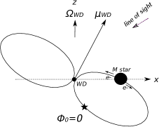
Figure 1.— Schematic view of the AR Sco system and the coordinate. The axes of the WD’s spin ($\vec{\Omega}_{WD}$) and orbital motion are assumed to be parallel and are defined as the $z$-axis. The $x$-axis is defined so that the observer is located with the plane made by the $x-$ and $z-$axes. We define the orbital phase $\Phi_{o}=0$ at the inferior conjunction of the M-type star. The magnetic axis $\vec{\mu}_{WD}$ is inclined from the spin axis.

2.1. Energy injection

Figure 1 illustrates the schematic view of the AR Sco system explored in this paper. As depicted in Figure 1, we define the zero orbital phase ($\Phi_{o}=0$) at the inferior conjunction of the orbit of the M-type star. We assume that a magnetic dissipation process eventually causes an ablation of the matter (hadrons and electrons) from the M-type star surface and an acceleration of the electrons to the relativistic speed. We estimate the dissipation rate from (Lai 2012; Buckley et al. 2017)

$$L_{B} = \frac{B^{2}}{8\pi}(4\pi R_{*}^{3}\delta)\Omega_{WD}\sim 2.8\times 10^{32}{\rm erg/s}$$ (1)

$$\times \left(\frac{\mu_{WD}}{10^{35}{\rm G~{}cm^{3}}}\right)^{2}\left(\frac{\delta}{0.01}\right)\left(\frac{R_{*}}{3\cdot 10^{10}{\rm cm}}\right)^{3}$$

$$\times \left(\frac{a}{8\cdot 10^{10}{\rm cm}}\right)^{-6}\left(\frac{P_{WD}}{117{\rm s}}\right),$$

where $\Omega_{WD}=2\pi/P_{WD}$, $\mu_{WD}$ is the WD’s magnetic dipole moment, $a$ is the separation between two stars, and $\delta\sim 0.01$ is the skin depth on the M-type star surface. We assume that most of the released energy is used to accelerate the electrons, and the typical Lorentz factor is estimated to be $\gamma_{0}\sim L_{B}/(\dot{N}_{e}m_{e}c^{2})$, where $\dot{N}_{e}$ is the rate of the electron injection in the closed magnetic field line region of the WD. Because of the charge conservation, we may assume that the number of injected electrons is equal to the proton number in the outflow. The dissipation of the magnetic energy forms the outflow of the matter from the stellar surface. If we denote the efficiency $\chi$ to form the outflow, the injection rate of the protons may be estimated from

$$\dot{N}_{p} \sim \frac{\dot{M}}{m_{p}}=\frac{\chi L_{B}}{\frac{1}{2}m_{p}v_{esc}^{2}}$$ (2)

$$\sim 5\times 10^{40}\chi\left(\frac{L_{B}}{10^{32}{\rm erg/s}}\right)\left(\frac{v_{esc}}{5\cdot 10^{7}{\rm cm/s}}\right)^{-2}{\rm/s},$$

where $v_{esc}=\sqrt{2GM_{*}/R_{*}}$ is the escape velocity. In the current study, $\chi\sim 10^{-5}$, which indicates that the typical Lorentz factor of $\gamma_{0}\sim 50$, will be chosen to fit the observed spectrum.

2.2. Equation of motion

With the Lorentz factor of $\gamma_{0}\sim 50$, the time scale of the synchrotron loss at around the M-type star is estimated as

$$\tau_{syn}\sim 400{\rm s}\left(\frac{\mu_{WD}}{10^{35}{\rm Gcm^{3}}}\right)^{-2}\left(\frac{a}{8\cdot 10^{10}{\rm cm}}\right)^{6}\left(\frac{\gamma_{0}}{50}\right)^{-1},$$

which is longer than the crossing time scale of $a/c\sim 2.7{\rm s}$. Hence, most of the injected electrons migrate to the inner magnetosphere of the WD. For the electrons moving along the magnetic field, the evolution of the Lorentz factor, $\gamma$, and the perpendicular momentum of an electron may be described by (Harding et al., 2005)

$$\frac{d\gamma}{dt}=-\frac{P_{\perp}^{2}}{t_{s}}$$ (3)

and

$$\frac{d}{dt}\left(\frac{P_{\perp}^{2}}{B}\right)=-2\frac{B}{t_{s}\gamma}\left(\frac{P_{\perp}^{2}}{B}\right)^{2},$$ (4)

where $B$ is the strength of the local dipole magnetic field, $t_{s}=3m_{e}^{3}c^{5}/(2e^{4}B^{2})$, and $P_{\perp}=\gamma\beta\sin\theta_{p}$, with $\beta=v/c$ and $\theta_{p}$ the pitch angle. We can see from the equation (4) that if the synchrotron cooling time scale $\tau_{s}=\gamma t_{s}/P_{\perp}^{2}$ is longer than the crossing time scale $\tau_{c}=r/c$, the magnetic mirror for the particle that starts from $r=a$ will occur at the point

$$r_{m}\sim a\sin\theta_{p,0}^{2/3},$$ (5)

where $\theta_{p,0}$ is the initial pitch angle. In this paper, we assume a pure magnetic dipole field of the WD, for simplicity.

For each magnetic field line that sweeps across the M-type star, the electrons are injected into both the northern and souther hemispheres from the position of the M-type star with a rate described by equation (2). The injected electrons with an initial pitch angle of $\theta_{p,0}>(R/a)^{3/2}$ cannot reach the stellar surface owing to the magnetic mirror effect, and they are trapped between two mirror points connected by the magnetic field line. Such a trapped electron will be eventually absorbed by the M-type star.

In the current model, the emission from the first magnetic mirror points mainly contribute to the observed emission, and the peak in the light curve is formed by the emission from the electrons that are injected when the magnetic pole points toward the companion (for details, see Takata et al. 2017). In Figure 1, for example, the north pole points toward the secondary, and emission from the electron injected into the southern hemisphere creates one peak. After 0.5 spin phase, the south pole points toward the secondary, and emission from the electron injected into the northern hemisphere creates another peak.

2.3. Radiation process

The observed nonthermal spectrum extends from the radio to the soft X-ray bands. To explain such a broadband spectrum, we assume that the acceleration process on the M-type star surface forms a power-law distribution in the electron’s Lorentz factor:

$$f(\gamma)=K_{0}\gamma^{-p},~{}\gamma_{min}\leq\gamma\leq\gamma_{max},$$ (6)

where $\gamma$ is the Lorentz factor of the electron. Takata et al. (2018) fit that broadband spectrum with a power-law index of $p=3$. We assume the minimum Lorentz factor as $\gamma_{min}\sim\gamma_{0}$, and estimate the maximum Lorentz factor from the condition that the synchrotron cooling time scale $t_{s}\sim 9m_{e}^{3}c^{5}/(4e^{4}B^{2}\gamma)$ is equal to the acceleration time scale of $t_{a}\sim\gamma m_{e}c/(\xi eB)$, where $\xi\leq 1$ represents the efficiency of the acceleration. In equation (6), the normalization $K_{0}$ is calculated from the condition that $\int\gamma m_{e}c^{2}f(\gamma)d\gamma=L_{B}$. The power per unit energy of the synchrotron radiation for each electron is calculated from (Rybicki & Lightman, 1986)

$$P_{syn}=\frac{\sqrt{3}e^{3}B\sin\theta_{p}}{hm_{e}c^{2}}F_{syn}\left(\frac{E}{E_{syn}}\right),$$ (7)

and

$$F_{syn}(x)=x\int_{x}^{\infty}K_{5/3}(y)dy,$$ (8)

where $E_{syn}=3he\gamma^{2}B\sin\theta_{p}/(4\pi m_{e}c)$, and $K_{5/3}$ is the modified Bessel function of order 5/3.

2.4. Polarization

Figure 2.— Definition of the angle of the linear polarization. $\vec{\Omega}_{p}$ and $\vec{n}_{o}$ are the direction of the projected spin of the axis seen from the observer and the direction of the observer seen from the WD, respectively. The direction of the polarization the P.A. $\chi$ increases in the counterclockwise, when looking at the source.

In this section, we describe our method to calculate the polarization of the synchrotron radiation from the trapped electrons. We apply the method developed by Takata et al. (2007), where we calculate the polarization characteristic of the synchrotron radiation from the electrons/positrons in the magnetosphere of the Crab pulsar. The unit vector of the velocity of the electron gyrating around the magnetic field line may be described by

$$\vec{n}_{e}=\pm\beta_{0}\cos\theta_{p}\vec{b}_{||}+\beta_{0}\sin\theta_{p}\vec{b}_{\perp}+\beta_{co}\vec{e}_{\phi},$$ (9)

where the vectors $\vec{b}_{||}=\vec{B}/B$, $\vec{b}_{\perp}$, and $\vec{e}_{\phi}$ represent the unit vectors along the magnetic field line, perpendicular to the magnetic field, and in the azimuthal (corotation with the WD) direction, respectively. The plus sign and minus sign in the first term consider the motion parallel and antiparallel to the magnetic field line, respectively. The second and third terms represent the gyration motion and the corotation motion with the WD’ spin, respectively. Since the direction of the gyration motion of the electron is counterclockwise as seen from the direction of the magnetic field, we may express the unit vector $\vec{b}_{\perp}$ as

$$\vec{b}_{\perp}=\cos\delta\phi_{g}\vec{k}+\sin\delta\phi_{g}\vec{b}\times\vec{k},$$ (10)

where $\vec{k}$ is any unit vector perpendicular to the magnetic field line and $\delta\phi_{g}$ represents the phase of the gyration motion ($0\leq\delta\phi_{g}<2\pi$). Since the electrons are relativistic, we calculate $\beta_{0}$ at each position from the condition that $|\vec{n}_{e}|=1$ and $\beta_{co}=\varpi/\varpi_{lc}$, where $\varpi_{lc}$ is the light cylinder radius of the WD. We assume that the emission direction of the relativistic electron coincides with the direction of the motion given by the equation (9).

We assume that after the electrons leave from the M-type star surface, they do not gain energy and just loose their energy via the synchrotron radiation. For the synchrotron radiation, the polarization vector is parallel to the direction of the centripetal acceleration for the gyration motion, and it is perpendicular to the direction of the local magnetic field. From equation (10), the polarization direction of the synchrotron radiation may be determined as

$$\vec{n}_{p}=-\sin\delta\phi_{g}\vec{k}+\cos\delta\phi_{g}\vec{b}\times\vec{k}.$$ (11)

In the calculation, we define the $z$-axis as the spin axis of the WD, which is assumed to be parallel to the axis of the orbital motion (see Figure 1). The $x$-axis is chosen so that the observer is located at the first quadrant in the ($x,z$) coordinate. With this coordinate system, the direction of the observer is expressed as

$$\vec{n}_{o}=\sin\theta_{o}\vec{e}_{x}+\cos\theta_{o}\vec{e}_{z},$$ (12)

where $\theta_{o}$ is the angle of the line of sight measured from the spin axis $\vec{e}_{x}$ and $\vec{e}_{z}$ are the unit vectors.

For each emission point, we consider the emission from all gyration phases, that is, $0\leq\delta\phi_{g}<2\pi$, and pick up the gyration phase that produces the synchrotron photon propagating toward the Earth. Then, we calculate the electric vector of the “observed” electromagnetic wave from

$$\vec{E}_{em,i}\propto\vec{n}_{p,i}-(\vec{n}_{o}\cdot\vec{n}_{p,i})\vec{n}_{o},$$ (13)

where “$i$” denotes each radiation. The degree of the linear polarization (hereafter P.D.) is estimated from (Rybicki & Lightman, 1986)

$$\Pi_{i}(E)=\frac{G_{syn}(x)}{F_{syn}(x)},$$ (14)

where $x=E/E_{syn}$, $F_{syn}$ is given by the equation (8) and $G_{syn}(x)=xK_{2/3}(x),$ with $K_{2/3}$ being the modified Bessel function of order 2/3.

To calculate the Stokes parameters, $Q_{i}$ and $U_{i}$, for each radiation, we define the polarization angle (hereafter P.A.) $\chi_{i}$ to be the angle between the polarization vector (13) and the direction of the spin axis projected on the observer sky, $\vec{\Omega_{p}}=\vec{\Omega}_{WD}-(\vec{n}_{o}\cdot\vec{\Omega}_{WD})\vec{n}_{o}$ (Figure 2),

$$\cos\chi_{i}=\frac{\vec{E}_{em,i}\cdot\vec{\Omega}_{p}}{|\vec{E}_{em,i}||\vec{\Omega}_{p}|}.$$ (15)

For the conventional definition, the P.A. $\chi_{i}$ increases in counterclockwise, when looking at the source. The Stokes parameters for each radiation are $Q_{i}(E)=\Pi_{i}(E)I_{i}(E)\cos 2\chi_{i}$ and $U_{i}(E)=\Pi_{i}(E)I_{i}(E)\sin 2\chi_{i}$, where $I_{i}(E)$ is the intensity. By collecting the observed radiation at each bin of the spin phase, $I(\phi_{s})=\sum I_{i}$, $Q(\phi_{s})=\sum Q_{i}$, and $U(\phi_{s})=\sum U_{i}$, we calculate the P.D. and P.A. for each bin from

$$P(\phi_{s})=\frac{\sqrt{Q^{2}(\phi_{s})+U^{2}(\phi_{s})}}{I(\phi_{s})},$$ (16)

and

$$\chi(\phi_{s})=\frac{1}{2}{\rm tan}^{-1}\left[\frac{Q(\phi_{s})}{U(\phi_{s})}\right],$$ (17)

respectively.

The current method cannot apply to estimate the circular polarization, since we consider only emission in the direction of the particle motion (see equation (9)). The synchrotron emission is in general elliptically polarized if the viewing angle deviates from the direction of the particle motion. For a power-law distribution of electrons, for example, the degree of the circular polarization of the synchrotron emission from the electrons with Lorentz factor $\gamma_{e}$ is given by (Sazonov 1972; Nava et al. 2016)

$$P_{circ}\sim-\frac{P_{lin}}{\gamma_{e}}\left(\cot\psi+\frac{1}{p+2}\frac{1}{Y(\psi)}\frac{dY(\psi)}{d\psi}\right),$$ (18)

where $P_{lin}$ is the degree of linear polarization, $\psi$ is the angle between the particle motion and the emission, and $Y(\psi)$ is the pitch-angle distribution. The ratio between circular and linear polarization is of the order of $1/\gamma_{e}$. Potter & Buckley (2018b), on the other hand, measure the circular polarization, peaking at a value of $\sim 3\%$. Such a high level of the circular polarization could imply a high level of pitch-angle anisotropy. A detailed calculation for the circular polarization is more complicated than that for the linear polarization since we have to take into account the emission in all directions relative to the particle motion and the pitch-angle distribution. We therefore focus on the linear polarization in this paper and will discuss the circular polarization in a subsequent study.

2.5. Pitch-angle distribution

Besides the energy distribution of the injected electrons, we also consider the effect of the distribution of the pitch angle. Within the current framework of the emission model, we will see in section 3 that the pitch-angle distribution sensitively affects the polarization characteristic. The distribution of the initial pitch angle of the relativistic electrons leaving the M-type star may be related to the acceleration process. For example, the standard acceleration model of the neutron star pulsar assumes that the electric field along the magnetic field line produces a relativistic particle. This acceleration process produces a population of the relativist particles with a small pitch angle. For the shock acceleration (e.g. in the magnetic turbulent), on the other hand, the accelerated particles would have various pitch angles (Achterberg et al. 2001; Kartavykh et al. 2016). In this study, we explore the pitch-angle distribution with a function form of

$$\frac{d\dot{N}_{e}}{d\cos\theta_{p,0}}=C_{0}+C_{1}\frac{{\rm exp}\left[-\frac{(\theta_{p,0}-\theta_{0})^{2}}{2\sigma_{0}^{2}}\right]}{A},\ ~{}~{}0<\theta_{p,0}<\pi/2,$$ (19)

where $A=\int_{0}^{\pi/2}{\rm exp}\left[-(\theta_{p,0}-\theta_{0})^{2}/(2\sigma_{0}^{2})\right]{\rm d}\cos\theta_{p,0}$. With the above equation, we assume that the initial pitch-angle distribution is composed of the isotropic component plus the anisotropic component described by the Gaussian-like function. In this study, the ratio of the constant factor $C_{0}/C_{1}$, the central value $\theta_{0}$, and the dispersion $\sigma_{0}$ are model-free parameters.

3. Results

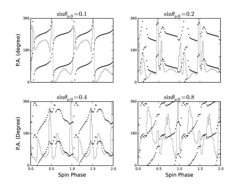
Figure 3.— Evolution of the polarization angle (filled circles) with spin phase for a specific initial pitch angle. The pulse profile for each case is plotted with the solid histogram. The results are calculated with $\Phi_{o}=0.5$, $\alpha=60^{\circ}$, and $\zeta=65^{\circ}$, respectively.

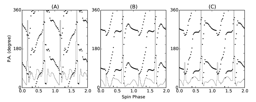
Figure 4.— Dependency of the polarization angle (filled circles) on the distribution of the initial pitch angle. (A) : Uniform distribution between $0\leq\theta_{p,0}\leq\pi/2$. (B) : Gaussian-like distribution with $\theta_{0}=0.2$rad and $\sigma_{0}$=0.2rad. (C) Distribution created by uniform component plus Gaussian-like component with $\theta_{0}=0.2$rad and $\sigma_{0}$=0.2rad and $C_{1}/C_{0}=1$ in equation (19). The results are calculated with $\alpha=60^{\circ}$, $\zeta=60^{\circ}$, and $\Phi_{o}=0.5$.

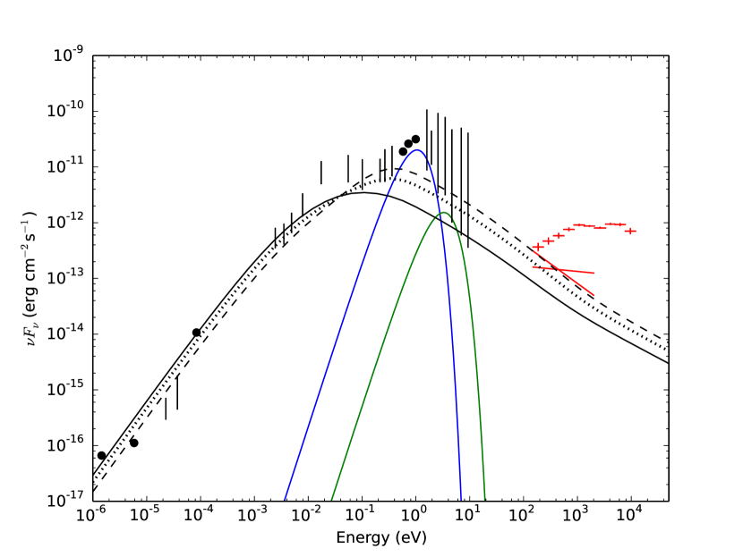
Figure 5.— Spectral energy distribution of AR Sco. The black solid, dashed, and dotted lines are the calculated spectrum with the initial pitch angle distributions for the panels (A), (B) and (C) in Figure 4, respectively. The data are taken from Takata et al. (2018) for X-ray bands and Marsh et al. (2016) for the radio/optical/UV bands. The red lines and plus signs represent the pulsed and nonpulsed components, respectively, of the X-ray emission. The blue and the green lines are the models for the blackbody emission from the M-type star and the WD, respectively. In the model calculation, the initial distribution in the Lorentz factor is assumed to be $p=3$.

The size of the M-type star ($R_{*}\sim 0.3R_{\odot})$ is not negligible compared to the size of the system ($a\sim R_{\odot}$). In the calculation, therefore, we inject the particles on the magnetic dipole field lines penetrating the day side of the M-type star (a half-hemisphere), and assume that the injection rate is the same for all magnetic field lines. In the calculation, we assume the inclination angle, $\alpha$, and the viewing angle, $\zeta$, measured from the spin axis of the WD. We will present the results for Earth viewing angle $\zeta<90^{\circ}$, because the observed swing direction of the P.A. predicts it, as discussed in section 4. The polarization characteristics predicted by $\alpha=\alpha_{0}$ and $\alpha=180^{\circ}-\alpha_{0}$ are identical from each other. In Figures 3, 4, and 6-8, the evolution of the P.A. (filled circles) along the spin phase is presented with the pulse profile (solid histograms)

3.1. P.A. and initial pitch angle

First, we examine the pulse profile and the swing of the P.A. predicted by a specific initial pitch angle, $\theta_{p,0}$. Figure 3 summarizes the evolution of the P.A. (filled circles) along the spin phase of the WD for the initial pitch angles of $\sin\theta_{p,0}=0.1$ (top left), 0.2 (top right), 0.4 (bottom left) and 0.8 (bottom right). The results are for the initial Lorentz factor $\gamma_{0}=100$, with which the electrons mainly produce the optical emission with the synchrotron radiation process. In each panel, the predicted pulse profile (solid histogram) is also plotted.

We find in Figure 3 that the calculated P.A. shows a large swing along the spin phase. For the pitch angle $\sin\theta_{p,0}=0.1$, for example, the pulse profile shows the double-peak structure and the P.A. swings $\sim 180^{\circ}$ at each peak. The total swing of the P.A. over one spin period is $\sim 360^{\circ}$, which can explain the observed swing angle. For a larger initial pitch angle, the calculated pulse profile is more complicated, with more than two peaks. This dependency of the pulse profile and the polarization characteristic are related to the contribution of the emission from the second and subsequent magnetic mirror points and the emission from both hemispheres. Equation (5) shows that the magnetic mirror occurs at the inner magnetosphere for the smaller pitch angle. This implies that a higher fraction of the initial energy of the particles is lost by the synchrotron radiation at the first mirror point. For $\sin\theta_{p,0}=0.1$ in Figure 3, for example, most of the initial particle energy is lost at the first mirror point, and the contribution of the emission from the subsequent mirror points makes small broad bumps between two main peaks. Since the photons detected at each spin phase bin are contributed by a smaller region in the magnetosphere, the angle of the linear polarization shows a monotonic increment along the spin phase.

For a larger initial pitch angle, since the magnetic mirroring occurs at a smaller magnetic field region (outer magnetosphere), a smaller fraction of the initial energy is released as the synchrotron radiation at the first mirror point. Hence, the emission from the subsequent mirror points also creates noticeable peaks in the calculated pulse profile, as we can see in Figure 3. A wider region in the magnetosphere contributes to the emission of each spin phase, and therefore the resultant evolution of the P.A. along the spin phase and the pulse profile become more complicated.

3.2. Pitch-angle distribution

Figure 4 summarizes the dependency of the polarization on the distribution of the initial pitch angle, by assuming the inclination angle $\alpha=60^{\circ}$ and the Earth viewing angle $\zeta=60^{\circ}$. The results are for the superior conjunction ($\Phi_{o}=0.5$). In the figure we can see that the predicted P.A. shows a large swing with the spin phase, but its evolution depends on the initial distribution. In panel (A), we assume a uniform distribution in $0\leq\theta_{p,0}\leq\pi/2$, that is, $C_{1}=0$ or $\sigma_{0}=\infty$ in equation (19), and we can see a complicated evolution of the P.A. with the spin phase. This is because the emission from high-order magnetic mirror points cannot be ignored in the pulse profiles. In the panel (B), we consider only the Gaussian component and assume that initial pitch angles concentrate at $\theta_{0}=0.2$ rad with a width of $\sigma_{0}=0.2$ rad. In such a case, more injected electrons lose their energy at the first magnetic mirror point, and the resultant polarization tends to increase with the spin phase. We can expect that as we increase the magnitude of $\sigma_{0}$, the calculated P.A. and pulse profile shift to those of the panel (A).

By comparing the calculated pulse profiles (solid histograms) in the panel (A) and panel (B), we find that the double-peak structure is more clearly shown in the pulse profile with the uniform distribution. In current model, a strong peak is created by each hemisphere, and the double peak structure is produced as a result of the contribution of the emission from both hemisphere. When the initial pitch angle concentrates to a smaller value, the emission from a half hemisphere could be missed by the observer, and the height of one peak is much lower than other peak, as the panel (B) indicates. To explain the observed double peak pulse profiles, therefore, a uniform component may be necessary.

In panel (C) of Figure 4, we assume that the initial pitch angle is described by the uniform component plus the Gaussian-like component, and we present the result with $C_{1}/C_{0}=1$, that is, we assume that the total particle number of the Gaussian component is equal to that of the uniform component. For the Gaussian component, we assume $\theta_{0}=0.2$ rad and $\sigma_{0}=0.2$ rad. In the figure, we can see that the pulse profile and evolution of the polarization angle are intermediate between those in the panels of (A) and (B). For example, we can see that the pulse height of the second peak (minor peak) is the lower than that in panel (A), but it is higher than that in panel (B). The evolution of the polarization angle with the spin phase is not as smooth as panel (B). We find that with current parameters of $\alpha=60^{\circ}$ and $\zeta=60^{\circ}$, $360^{\circ}$ of the P.A. swing along the spin phase can be reproduced with $C_{1}/C_{0}\geq 1$. Our model therefore suggests that the particle acceleration on the M-type star surface produces more relativistic electrons having smaller pitch angle. As a conclusion of this section, the two component model (panel C) of the initial pitch-angle distribution explains better both observed double peak structure and polarization characteristics.

The predicted anisotropy of the initial pitch angle distribution might be consistent with the observed circular polarization, peaking at a value of $\sim 3\%$ (Potter & Buckley, 2018b). Such a high level of the circular polarization would require a high level of pitch-angle anisotropy. The calculation of the circular polarization based on the current model will be done in a subsequent study.

Figure 5 compares the model spectra for the panels (A) (solid line), (B) (dashed line), and (C) (dotted line) in Figure 4. In the calculation, we assume $p=3$ for the power-law distribution in the initial Lorentz factor to explain the observed spectra of the pulsed emission in optical/UV and soft X-ray bands. In this figure, we can see that the predicted spectrum becomes harder if the initial pitch-angle distribution is biased in the smaller angle. This can be understood because the mirror point for an electron with a smaller initial pitch angle is closer to the stellar surface, and therefore the synchrotron emission at the mirror point is harder. As we can see in the figure, the observed spectra cannot tightly constrain the initial pitch-angle distribution.

3.3. Evolution with orbital phase

Figure 6 summarizes the dependency of the evolution of the linear polarization (filled circles) and the pulse profiles (histograms) on the orbital phase. For the pulse profile, we can see that the position of the peak shifts with the orbital phase. In the current model, the pulse peaks are mainly created by the emission of the electrons injected when the magnetic axis of the WD points toward the M-type star (Takata et al., 2017), and hence the pulse peak shifts with the orbital motion of the M-type star.

We see in the figure that the polarization characteristics and the pulse profile depend on the orbital phase. At the orbital phase $\Phi_{o}=0.25$ (descending node of the orbit of the M-type star) and 0.5 (superior conjunction), for example, the P.A. tends to increase with the spin phase, while at $\Phi_{o}=0$ (inferior conjunction) and 0.75 (ascending node), the swing of the P.A. changes its direction at spin phase $0.6-0.7$. For $\Phi_{o}=0$, we find a small second peak in the calculated pulse profile. Since the M-type star is between Earth and the WD, the electrons leaving from the M-type star move away from Earth. As a result, the strong emission from one hemisphere may not point toward Earth.

We note that the predicted characteristics of the P.A. and the pulse profiles at $\Phi_{o}=0.25$ and $\Phi_{o}=0.75$ are different from each other; nevertheless, the positions of the M-type star are symmetric relatively to the axis made by Earth and the WD. The difference originates from the direction of the WD’s spin. In the current study, we anticipate that the direction of the WD’s spin is parallel to the axis of the orbital motion. At $\Phi_{o}=0.25$, since the WD’s magnetic field sweeps across the M-type star from the Earth side to the backside, the trapped electrons initially move away from the Earth. This makes a pulse profile broader. At $\Phi_{o}=0.75$, the magnetic field sweeps across the M-type star from the backside to the Earth side, and therefore the trapped electrons move initially toward the Earth. The emitted photons and the emitting electrons that continuously produce the photons may initially move in the same direction. This tends to shorten the difference in the arrival times of the different photons and tends to make a sharper peak.

We mention that the current calculation has some discrepancies from the observations. For example, the observed optical/UV pulse profile evolves with the orbital phase. With OM data of the $XMM$-Newton telescope, we (Takata et al. 2018) show that the shape of the pulse profile rapidly changes at around $\Phi_{o}=0$ and a small second peak structure is found in the pulse profile at around $\Phi_{o}=0.1$. This feature is similar to the current model. On the other hand, the observed pulse profile at $\Phi_{0}=0.5-0.6$ is described by a broad pulse profile with no clear second peak, while the current pulse profile shows a double-peak structure. For the optical polarization, Potter & Buckley (2018b) show that the total swing of the P.A. over the spin phase is $360^{\circ}$ and does not depend on the orbital phase. As we can see in Figure 6, the current calculation predicts that the total swing of the P.A. at $\Phi_{O}=0$ and $0.75$ phases is less than $360^{\circ}$. A fine-tuning for parameters (e.g. initial Lorentz factor and pitch-angle distribution and system geometry) will be required to obtain a total $360^{\circ}$ swing for the whole orbital phase. This difference between the model and observation could also indicate that the realistic geometry and structure of the magnetosphere (e.g. magnetic field structure) are more complicated comparing to current simple treatment. For example, the dipole field approximation could be a very rough treatment owing to the interaction with the companion star.

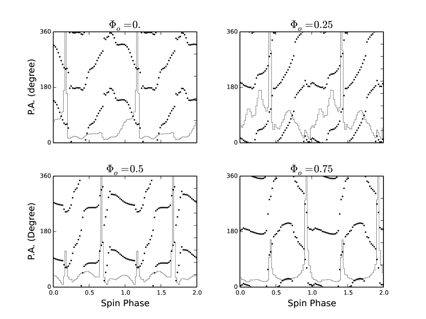
Figure 6.— Evolution of the P.A. swing (circles) and the pulse profile (histograms) with the orbital phase. The magnetic inclination angle and viewing angle are $\alpha=60^{\circ}$ and $\zeta=60^{\circ}$, respectively. The phase $\Phi_{0}=0$ corresponds to the inferior conjunction of the M-type star, and $\phi_{s}=0$ in all panels corresponds the spin phase at which the magnetic axis is directed toward the Earth. The results are for $C_{0}=C_{1}$ with $\theta_{0}=0.2$ and $\sigma_{0}=0.2$.

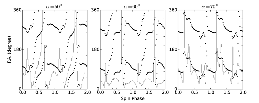
Figure 7.— Dependency of the P.A. swing and the pulse profiles on the magnetic inclination angle. The results are for $\Phi_{o}=0.5$, the Earth viewing angle $\zeta=60^{\circ}$, and $C_{0}=C_{1}$.

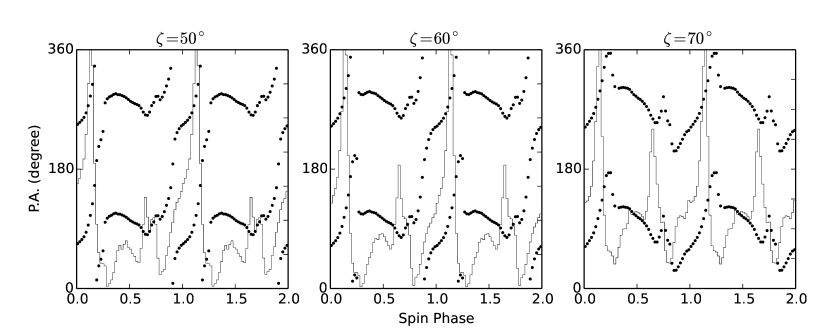
Figure 8.— Dependency of the P.A. swing and the pulse profiles on the Earth viewing angle. The results are for $\Phi_{o}=0.5$, the magnetic inclination angle $\alpha=50^{\circ}$, and $C_{0}=C_{1}$.

3.4. Dependency on the geometry

Within the current framework of the model, we find that the calculated polarization characteristic depends on the viewing geometry. For example, Figures 7 and 8 summarize the dependency of the inclination angle of the magnetic axis of the WD and the Earth viewing angle, respectively. Using the orbital phase $\Phi_{o}=0.5$, the Earth viewing angle $\zeta=60^{\circ}$, and $C_{0}=C_{1}$, Figure 7 compares the results for $\alpha=50^{\circ}$ (left panel), $60^{\circ}$ (middle panel), and $70^{\circ}$ (right panel). In the figure, we can see the tendency of an increase in the P.A. along the spin phase for inclination angles $\alpha=50^{\circ}$ and $60^{\circ}$, while we see a complicated evolution for $\alpha=70^{\circ}$. For $\alpha=70^{\circ}$, we can see many sharp peaks in the calculated pulse profile. This shows that with a specific Earth viewing angle, the emission from the second and subsequent mirror points also contributes to the observed emission and produces a complicated evolution of the P.A. swing. We find therefore that the current model prefers the magnetic inclination angle of $\alpha=50^{\circ}-60^{\circ}$ to produce a $360^{\circ}$ swing of the P.A. along the spin phase. For a nearly aligned rotator, on the other hand, the model does not predict the double-peak structure, as discussed in Takata et al. (2017).

In Figure 8, we summarize the dependency of the viewing angle on the polarization characteristics with $\alpha=50^{\circ}$, $\Phi_{o}=0.5$, and $C_{0}=C_{1}$. With these parameters, we can see in the figure that a smaller viewing angle ($\zeta=50^{\circ}$ and $\zeta=60^{\circ}$) shows a monotonic increase in the P.A. with the spin phase, and for a larger viewing angle (right panel for $\zeta=70^{\circ}$), the P.A. changes its swing direction at a spin phase. This dependency on the viewing angle also comes from the dependency of the contribution from both hemispheres. From the pulse profiles (histograms in the figure), we can see that the height of the second peak at $\phi_{s}\sim 0.7$ increases as the Earth viewing angle increases. This is related to the fact that when we look at the system from an angle closer to the equator, the difference in the contribution of the emission from the two hemispheres decreases (for the observer with $\zeta=90^{\circ}$, the contributions from two hemispheres are even). This makes the evolution of the P.A. swing and the pulse profile more complicated. For viewing angle $\zeta\sim 0^{\circ}$, on the other hand, we expect no or smaller modulation of the observed flux with the spin/beat phase. As a result, the current model prefers the Earth viewing angle, $\zeta=50^{\circ}-60^{\circ}$, as well as the magnetic inclination angle $\alpha=50^{\circ}-60^{\circ}$.

3.5. Degree of linear polarization

The observed optical emission will be composed of two components: (1) thermal emission from the M-type star surface and (2) nonthermal emission from the relativistic particles, as Figure 5 indicates. It has been observed that the pulsed fraction, which is defined by the equation ($f_{max}-f_{min})/(f_{max}+f_{min})$, with $f_{max}$ and $f_{min}$ being the maximum and minimum counts in the pulse profile, depends on the photon energy bands and on the orbital phase; it becomes maximum around the inferior conjunction (hereafter INFC) of the M-type star’s orbit and minimum around the superior conjunction (hereafter SUPC). For example, the pulsed fraction of the UV emission is $\sim 70$% at the INFC and about $\sim 40$% at the SUPC (Takata et al., 2018). Moreover, it has been observed that the P.D. of the optical emission also depends on the orbital phase and may be related to the pulsed fraction. Buckley et al. (2017) report that the the P.D. can reach at the level of $\sim 30-40$% at the orbital phase $\Phi_{ob}=0-0.2$, while it is $10-20$% at $\Phi_{ob}\sim 0.4-0.6$. These evolutions of the pulsed fraction and P.D. would reflect (i) an evolution of the linear counts (synchrotron emission) and/or (ii) an evolution of contribution of the emission from the day side of the M-type star.

Figure 9 shows typical P.D. predicted by the current model. If we consider only the synchrotron emission (blue line), the pulsed fraction is $\sim 80$% and the P.D. can reach $\sim 60$%, which is higher than the observed one, P.D.$\leq 40$%. We therefore expect that the contribution of the unpolarized emission from the star reduces the P.D. To examine the effect of the thermal emission on the P.D., we assume that the thermal emission from the M-type stellar surface is unpolarized. Then, we add the unpolarized emission as a DC emission to reduce the pulsed fraction to $10$%. The calculated P.D. (red line in the figure) is significantly reduced to $\leq 10$% and has a peak at the pulse peak, which is roughly consistent with the observation around $\Phi_{o}\sim 0.5$.

From Buckley et al. (2017) and Potter & Buckley (2018b), for example, we can see that the linear counts averaged over the spin phase are almost constant between 0.1 and 0.5 orbital phase. However, the maximum P.D. of $\sim 40$% at around 0.1-0.2 orbital phase is higher than $\sim 20$% at around 0.4-0.5 orbital phase. This difference in the P.D. would be attributed by the different contributions of the stellar emission to the total emission. Since the contribution of the emission from the M-type star to the total emission at 0.1-0.2 orbital phase is smaller than that at 0.4-0.5 orbital phase, the P.D. at 0.1-0.2 orbital phase is larger than that at 0.4-0.5 orbital phase.

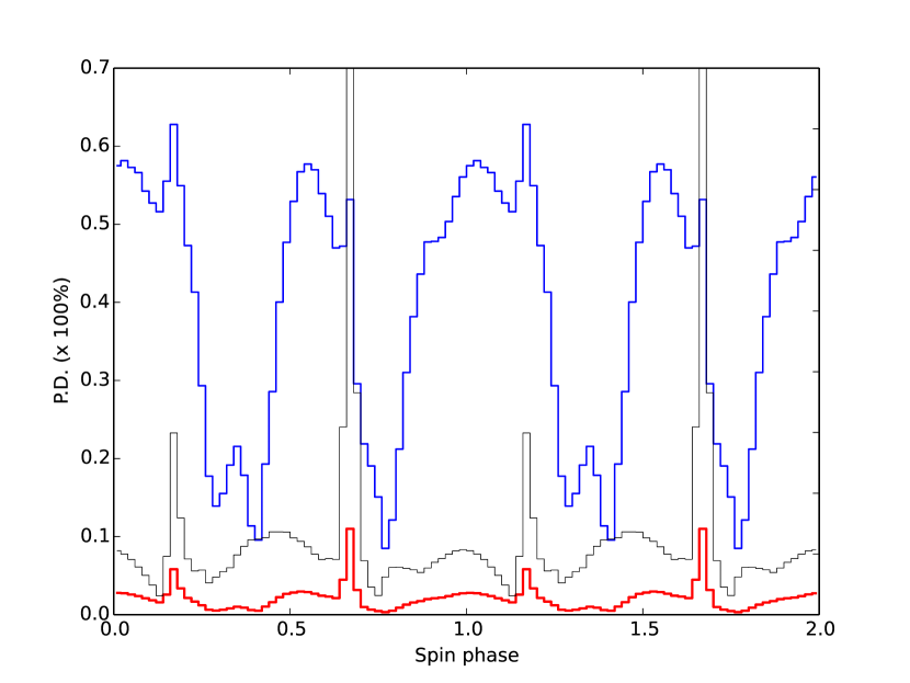
Figure 9.— Typical P.D.. The blue line shows the result without the contribution of the emission from the M-type star, for which the unpolarized emission is assumed. The red line considers the contribution of the unpolarized emission to reduce the pulsed fraction to 10%. The results are for $\Phi_{o}=0.5$, $\alpha=60^{\circ}$, $\zeta=60^{\circ}$, and $C_{0}=C_{1}=1$.

4. Discussion and Summary

The swing direction of the observed linear polarization will be able to constrain the viewing geometry. In the previous section, we assumed that the viewing angle is smaller than $\zeta<90^{\circ}$ measured from the WD’s spin axis. This condition is necessary to explain the swing direction of the observed P.A. with the spin phase, that is, counterclockwise. For the viewing angle with $\zeta>90^{\circ}$, the expected direction is clockwise. The difference in the swing directions for the two viewing angles mainly comes from the difference in the directions of the magnetic field line projected on the sky. We note that for a specific viewing angle, the inclination angles $\alpha=\alpha_{0}$ and $\alpha=180^{\circ}-\alpha_{0}$ do not make any difference in the morphology of the pulse profile and the polarization characteristics, since the directions of the magnetic field lines projected on the sky for the two inclination angles are identical. Hence, the required condition that $\zeta<90^{\circ}$ does not depend on whether the magnetic inclination angle is larger or smaller than $90^{\circ}$.

In Figure 3 of Buckley et al. (2017), we can see the spin phase where the swing angle of the observed P.A. is small (e.g. $\phi_{s}=0.1-0.5$ in the right panel of the figure). In our results, a similar trend can be seen in the calculated evolution of the P.A. In Figure 6, for example, we find a spin phase where the direction of the linear polarization is almost constant at P.A.$\sim 90^{\circ}$ for $\Phi_{o}=0.5$ and at P.A.$\sim 0^{\circ}$ (and $180^{\circ}$) for $\Phi_{o}$=0, 0.25, and 0.75. Figure 7 and 8 also suggest that the P.A. of the flat region does not depend on the inclination angle and viewing angle. In our definition, the direction of the P.A.$=0^{\circ}$ (or $90^{\circ}$) is parallel (or perpendicular) to the direction of the projected spin axis. Therefore, a detailed comparison between the observed and calculated P.A. may enable us to determine the direction of the spin axis of the WD projected on the sky.

The double-peak structure of the pulse profile, the large P.D., and the large swing of the polarization angle of the optical emission from AR Sco resemble those of the Crab pulsar (Kanbach et al., 2005). Based on our emission model, however, we would like to say that although the emission process is the synchrotron radiation for the two cases, the particle acceleration/emission regions are very different from each other. It has usually been argued that the nonthermal emission of the neutron star pulsar originates from the open field line region, for which the magnetic field lines extend beyond the light cylinder that is defined by the axial distance $\varpi_{lc}=P_{s}c/2\pi$ ($\sim 1.5\times 10^{8}{\rm cm}$ for the Crab and $5.6\times 10^{11}{\rm cm}$ for the WD in AR Sco), and the emission takes place around the light cylinder. For the AR Sco, the M-type star orbits at $a\sim 8\times 10^{10}{\rm cm}$ inside the light cylinder of the WD, and hence the emission probably originates from the closed magnetic field line region, as we have discussed in this paper. For the Crab pulsar, the pair-creation process of the GeV gamma-rays creates the electrons and positrons that emit the synchrotron photons. (Takata et al. 2007; Takata & Chang 2007). These secondary pairs will have a small pitch angle of $\sin\theta_{p}\sim 0.1$, and the emission from them covers a part of the sky. A special relativistic effect (e.g. flight time and aberration) makes a peak in the observed pulse profile of the Crab pulsar. In the current model of the AR Sco, the mirror point of the closed magnetic field is the main emission region, and the special relativistic effect is less important to form a peak in the pulse profile.

In summary, we have studied the linear polarization of the nonthermal optical emission from AR Sco with the model developed by Takata et al. (2017). In the model, the relativistic electrons trapped by the closed magnetic field line region produce the nonthermal emission with the synchrotron process. We have found that the calculated linear polarization can have a large swing through the spin phase, although the evolution of the P.A. with the spin phase depends on various factors (e.g. orbital phase, initial pitch-angle distribution, and viewing geometries). The total swing of the observed P.A. over the spin period can be $360^{\circ}$. To explain the large swing angle and the double-peak structure of the pulse profile, the current model suggests (1) an isotropy of the initial pitch-angle distribution, which is biased to a smaller value, and (2) a moderate magnetic inclination angle $(\alpha\sim 50^{\circ}-60^{\circ}$) and the Earth viewing angle $(\zeta\sim 50^{\circ}-60^{\circ})$. We have also shown that the P.D. can reach to $\sim 60$%, if the emission from the relativistic electrons dominates the emission from the stellar surface. The different contribution of the emission from the M-type star on the observed optical emission will explain the evolution of the observed P.D. with the orbital phase. We have discussed that the origin of the nonthermal emission of the AR Sco is different from the neutron-star-pulsar-like emission process. However, AR Sco is only a sample of the pulsed nonthermal emission from the magnetic WD. More samples will be necessary to understand the nonthermal nature of the magnetic WDs and the similarity/dissimilarity with the non-thermal emission from neutron star pulsars.

We express our appreciation to an anonymous referee for useful comments and suggestions. J.T. is supported by NSFC grants of the Chinese Government under 11573010, 11661161010, U1631103 and U1838102. K.S.C. is supported by GRF grant under 17302315.

References

- Achterberg et al. (2001) Achterberg, A. and Gallant, Y. A. and Kirk, J. G. and Guthmann, A. W., 2017, MNRAS, 328, 393
- Bednarek (2018) Bednarek, W., 2018, MNRAS, Letter, 476, 10
- Buckley et al. (2017) Buckley, D. A. H., Meintjes, P. J., Potter, S. B., Marsh, T. R., Gänsicke, B. T., 2017, Nature Astronomy, 1, 0029
- Ferrario et al. (2015) Ferrario, L., de Martino, D., Gnsicke, B. T., 2015, SSRv, 191, 111
- Geng et al. (2016) Geng, J.-J. and Zhang, B. and Huang, Y.-F., 2016, ApJ, 831, L10
- Harding et al. (2005) Harding, A. K., Usov, V. V. and Muslimov, A. G., 2005, ApJ, 622, 531
- Kanbach et al. (2005) Kanbach, G. and Słowikowska, A. and Kellner, S. and Steinle, H., 2005, in AIP Conf. Proc. 801, Astrophysical Sources of High Energy Particles and Radiation, ed. T. Bulik, B. Rudak, & G. Madejski (Melville, NY: AIP), 306
- Kartavykh et al. (2016) Kartavykh, Y. Y. and Dröge, W. and Gedalin, M., 2016, ApJ, 820, 24
- Katz (2017) Katz, J. I., 2017, ApJ, 835, 150
- Lai (2012) Lai, D., 2012, ApJ, 757, L3
- Littlefield et al. (2017) Littlefield, C., Garnavich, P., Kennedy, M., Callanan, P., Shappee, B., Holoien, T., 2017, ApJ, 845, 7
- Marsh et al. (2016) Marsh, T. R., Gänsicke, B. T., Hümmerich, S., et al. 2016, Nature, 537, 374
- Nava et al. (2016) Nava, L., Nakar, E., & Piran, T. 2016, MNRAS, 455, 1594
- Potter & Buckley (2018b) Potter, S. B. and Buckley, D. A. H., 2018b, MNRAS, 481, 2384
- Potter & Buckley (2018a) Potter, S. B. and Buckley, D. A. H., 2018a, MNRAS, 478L, 78
- Rybicki & Lightman (1986) Rybicki, G. B. and Lightman, A. P., 1986, Radiative Processes in Astrophysics, by George B. Rybicki, Alan P. Lightman, pp. 400. ISBN 0-471-82759-2. Wiley-VCH , June 1986.
- Sazonov (1972) Sazonov, V. N., 1972, Ap&SS, 19, 25
- Stanway et al. (2018) Stanway, E. R.,Marsh, T. R., Chote, P., Gänsicke, B. T. Steeghs, D., Wheatley, P. J., 2018, A&A, 611, 66
- Stiller et al. (2018) Stiller, R. A., Littlefield, C., Garnavich, P., et al. 2018, AJ, 156, 150
- Takata et al. (2007) Takata, J., Chang, H.-K. , Cheng, K. S., 2007, ApJ, 656, 1044-1055
- Takata & Chang (2007) Takata, J., Chang, H.-K., 2007, ApJ, 670, 677
- Takata et al. (2017) Takata, J., Yang, H., Cheng, K.-S., 2017, ApJ, 851, 143
- Takata et al. (2018) Takata, J., Hu, C.-P., Lin, L. C. C., Tam, P. H. T., Pal, P. S., Hui, C. Y., Kong, A. K. H., Cheng, K. S., 2018, ApJ, 853. 106