Recurrent Event Network: Autoregressive Structure Inference over Temporal Knowledge Graphs

Abstract

Knowledge graph reasoning is a critical task in natural language processing. The task becomes more challenging on temporal knowledge graphs, where each fact is associated with a timestamp. Most existing methods focus on reasoning at past timestamps and they are not able to predict facts happening in the future. This paper proposes Recurrent Event Network (RE-Net), a novel autoregressive architecture for predicting future interactions. The occurrence of a fact (event) is modeled as a probability distribution conditioned on temporal sequences of past knowledge graphs. Specifically, our RE-Net employs a recurrent event encoder to encode past facts, and uses a neighborhood aggregator to model the connection of facts at the same timestamp. Future facts can then be inferred in a sequential manner based on the two modules. We evaluate our proposed method via link prediction at future times on five public datasets. Through extensive experiments, we demonstrate the strength of RE-Net, especially on multi-step inference over future timestamps, and achieve state-of-the-art performance on all five datasets.

1 Introduction

Knowledge graphs (KGs), which store real-world facts, are vital in various natural language processing applications Bordes et al. (2013); Schlichtkrull et al. (2018); Kazemi et al. (2019). Due to the high cost of annotating facts, most knowledge graphs are far from complete, and thus predicting missing facts (a.k.a., knowledge graph reasoning) becomes an important task. Most existing efforts study reasoning on standard knowledge graphs, where each fact is represented as a triple of subject entity, object entity and the relation between them. However, in practice, each fact may not be true forever, and hence it is useful to associate each fact with a timestamp as a constraint, yielding a temporal knowledge graph (TKG). Fig. 1 shows example subgraphs of a temporal knowledge graph. Despite the ubiquitousness of TKGs, methods for reasoning over such kind of data are relatively unexplored.

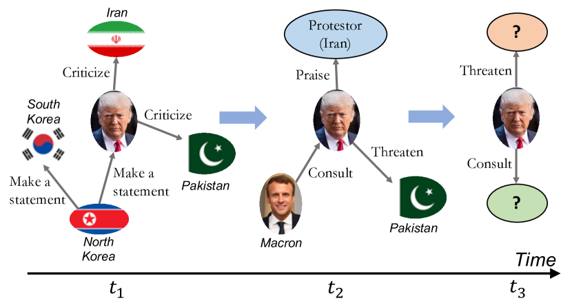
Figure 1: Example temporal knowledge subgraphs. Each edge or interaction between entities is associated with temporal information and a set of interactions build a multi-relational graph at each time. Our task is to predict interactions and build graphs at future times.

Given a temporal knowledge graph with timestamps varying from $t_{0}$ to $t_{T}$, TKG reasoning primarily has two settings - interpolation and extrapolation. In the interpolation setting, new facts are predicted for time $t$ such that $t_{0}\leq t\leq t_{T}$ García-Durán et al. (2018); Leblay and Chekol (2018); Dasgupta et al. (2018). In contrast, extrapolation reasoning, as a less studied setting, focuses on predicting new facts (e.g., unseen events) over timestamps $t$ that are greater than $t_{T}$ (i.e., $t>t_{T}$). The extrapolation setting is of particular interests in TKG reasoning as it helps populate the knowledge graph over future timestamps and facilitates forecasting emerging events Muthiah et al. (2015); Phillips et al. (2017); Korkmaz et al. (2015).

Recent attempts to solve the extrapolation TKG reasoning problem are Know-Evolve (Trivedi et al., 2017) and its extension DyRep (Trivedi et al., 2019), which predict future events assuming ground truths of the preceding events are given at inference time. As a result, these methods are unable to predict events sequentially over future timestamps without ground truths of the preceding events–i.e., a practical requirement when deploying such reasoning systems for event forecasting Morstatter et al. (2019). Moreover, these approaches do not model concurrent events occurring within the same time window (e.g., a day, or 12 hours), despite their prevalence in real-world event data Boschee et al. (2015); Leetaru and Schrodt (2013). Thus, it is desirable to have a principled method that can extrapolate graph structures over future timestamps by modeling the concurrent events within a time window as a local graph.

To this end, we propose an autoregressive architecture, called Recurrent Event Network (RE-Net), for modeling temporal knowledge graphs. Key ideas of RE-Net are based on: (1) predicting future events over multiple time stamps can be formulated as a sequential and multi-step inference problem; (2) temporally adjacent events may carry related semantics and informative patterns, which can further help predict future events (i.e., temporal information); and (3) multiple events may co-occur within the same time window and exhibit structural dependencies between entities (i.e., local graph structural information).

Given these observations, RE-Net defines the joint probability distribution of all events in a TKG in an autoregressive fashion. The probability distribution of the concurrent events at the current time step is conditioned on all the preceding events (see Fig. 2 for an illustration). Specifically, a recurrent event encoder summarizes information of the past event sequences, and a neighborhood aggregator aggregates the information of concurrent events within the same time window. With the summarized information, our decoder defines the joint probability of a current event. Inference for predicting future events can be achieved by sampling graphs over time in a sequential manner.

We evaluate our proposed method on five public TKG datasets via a temporal (extrapolation) link prediction task, by testing the performance of multi-step inference over time. Experimental results demonstrate that RE-Net outperforms state-of-the-art models of both static and temporal knowledge graph reasoning, showing its better capability to model temporal, multi-relational graph data. We further show that RE-Net can perform effective multi-step inference to predict unseen entity relationships in a distant future.

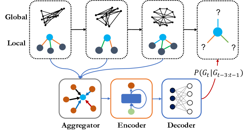
Figure 2: Illustration of the Recurrent Event Network architecture. The aggregator encodes the global graph structure and the local neighborhood, capturing global and local information respectively. The recurrent event encoder updates its state with the sequence of encoded representations of graph structures. The MLP decoder defines the probability of a current graph.

2 Problem Formulation

We first describe notations for building our model and problem definition, and then we define the joint distribution of temporal events.

Notations and Problem Definition. We consider a temporal knowledge graph as a multi-relational, directed graph with time-stamped edges between nodes (entities). An event is defined as a time-stamped edge, i.e., (subject entity, relation, object entity, time) and is denoted by a quadruple $(\mathrm{s},\mathrm{r},\mathrm{o},t)$ or $(\mathrm{s}_{t},\mathrm{r}_{t},\mathrm{o}_{t})$. We denote a set of events at time $t$ as ${G}_{t}$. In our setup, the timestamps are discrete integers and used for the relative order of graphs or events. A TKG is built upon a sequence of event quadruples ordered ascending based on their timestamps, i.e., $\{G_{t}\}_{t}=\{(\mathrm{s}_{i},\mathrm{r}_{i},\mathrm{o}_{i},t_{i})\}_{i}$ ($t_{i}<t_{j},\forall i<j$), where each time-stamped edge has a direction pointing from the subject entity to the object entity. The goal of learning generative models of events is to learn a distribution $p(G)$ over TKGs, based on a set of observed event sets $\{G_{1},...,G_{t}\}$.

Approach Overview. The key idea of our approach is to learn temporal dependency from the sequence of graphs and local structural dependency from the neighborhood (Fig. 2). Formally, we represent TKGs as sequences, and then build an autoregressive generative model on the sequences. To this end, RE-Net defines the joint probability of concurrent events (or a graph), which is conditioned on all the previous events. Specifically, RE-Net consists of a Recurrent Neural Network (RNN) as a recurrent event encoding module and a neighborhood aggregation module to capture the information of graph structures. We first start with the definition of joint distribution of temporal events.

Modeling Joint Distribution of Temporal Events. We define the joint distribution of all the events $G=\{G_{1},...,G_{T}\}$ in an autoregressive manner. Basically, we decompose the joint distribution into a sequence of conditional distributions, $p(G_{t}|G_{t-m:t-1})$), where we assume the probability of the events at a time step, $G_{t}$, depends on the events at the previous $m$ steps, $G_{t-m:t-1}$. For each conditional distribution $p(G_{t}|G_{t-m:t-1})$, we further assume that the events in $G_{t}$ are mutually independent given the previous events $G_{t-m:t-1}$. In this way, the joint distribution can be rewritten as follows:

$$p(G)=\prod_{t}\prod_{(\mathrm{s}_{t},\mathrm{r}_{t},\mathrm{o}_{t})\in G_{t}}p(\mathrm{s}_{t},\mathrm{r}_{t},\mathrm{o}_{t}|G_{t-m:t-1})\\ =\prod_{t}\prod_{(\mathrm{s}_{t},\mathrm{r}_{t},\mathrm{o}_{t})\in G_{t}}p(\mathrm{s}_{t}|G_{t-m:t-1})\cdot p(\mathrm{r}_{t}|\mathrm{s}_{t},G_{t-m:t-1})\\ \cdot p(\mathrm{o}_{t}|\mathrm{s}_{t},\mathrm{r}_{t},G_{t-m:t-1}).$$ (1)

From these probabilities, we generate triplets as follows. Given all the past events $G_{t-m:t-1}$, we first sample a subject entity $\mathrm{s}_{t}$ through $p(\mathrm{s}_{t}|G_{t-m:t-1})$. Then we generate a relation $\mathrm{r}_{t}$ with $p(\mathrm{r}_{t}|\mathrm{s}_{t},G_{t-m:t-1})$, and finally the object entity $\mathrm{o}_{t}$ is generated by $p(\mathrm{o}_{t}|\mathrm{s}_{t},\mathrm{r}_{t},G_{t-m:t-1})$.

Next, we introduce how these probabilities are defined and parameterized in our method.

3 Recurrent Event Network

In this section, we introduce our proposed method, Recurrent Event Network (RE-Net). RE-Net consists of a Recurrent Neural Network (RNN) as a recurrent event encoder (Sec. 3.1) for temporal dependency and a neighborhood aggregator (Sec. 3.2) for graph structural dependency. We also discuss parameter learning of RE-Net and define multi-step inference for distant future by sampling intermediate graphs in a sequential manner (Sec. 3.3).

3.1 Recurrent Event Encoder

To parameterize the probability for each event, RE-Net introduces a set of global representations as well as local representations. The global representation $\boldsymbol{H}_{t}$ summarizes the global information from the entire graph until time stamp $t$, which reflects the global preference on the upcoming events. In contrast, the local representations focus more on each subject entity $\mathrm{s}$ or each pair of subject entity and relation $(\mathrm{s},\mathrm{r})$, which capture the knowledge specifically related to those entities and relations. We denote the above local representations as $\boldsymbol{h}_{t}(\mathrm{s})$ and $\boldsymbol{h}_{t}(\mathrm{s},\mathrm{r})$, respectively. The global and local representations capture different aspects of knowledge from the knowledge graph, which are naturally complementary, allowing us to model the generative process of the graph in a more effective way.

Based on the above representations, RE-Net parameterizes $p(\mathrm{o}_{t}|\allowbreak\mathrm{s},\mathrm{r},G_{t-m:t-1})$ in the following way:

$$p(\mathrm{o}_{t}|\mathrm{s},\mathrm{r},G_{t-m:t-1})\propto\exp\left([\boldsymbol{e}_{\mathrm{s}}:\boldsymbol{e}_{\mathrm{r}}:\boldsymbol{h}_{t-1}(\mathrm{s},\mathrm{r})]^{\top}\cdot\boldsymbol{w}_{\mathrm{o}_{t}}\right),$$ (2)

where $\boldsymbol{e}_{\mathrm{s}},\boldsymbol{e}_{\mathrm{r}}\in\mathbb{R}^{d}$ are learnable embedding vectors specified for subject entity $\mathrm{s}$ and relation $\mathrm{r}$. $\boldsymbol{h}_{t-1}(\mathrm{s},\mathrm{r})\in\mathbb{R}^{d}$ is the local representation for $(\mathrm{s},\mathrm{r})$ obtained at time stamp $(t-1)$. Intuitively, $\boldsymbol{e}_{\mathrm{s}}$ and $\boldsymbol{e}_{\mathrm{r}}$ can be understood as static embedding vectors for subject entity $\mathrm{s}$ and relation $\mathrm{r}$, whereas $\boldsymbol{h}_{t-1}(\mathrm{s},\mathrm{r})$ is dynamically updated at each time stamp. By concatenating both the static and dynamic representations, RE-Net can effectively capture the semantic of $(\mathrm{s},\mathrm{r})$ up to time stamp $(t-1)$. Based on that, we further compute the probability of different object entities $\mathrm{o}_{t}$ by passing the encoding into our multi-layer perceptron (MLP) decoder. We define the MLP decoder as a linear softmax classifier parameterized by $\{\boldsymbol{w}_{\mathrm{o}_{t}}\}$.

Similarly, we define probabilities for relations and subjects as follows:

$$p(\mathrm{r}_{t}|\mathrm{s},G_{t-m:t-1}) \propto\exp\left([\boldsymbol{e}_{\mathrm{s}}:\boldsymbol{h}_{t-1}(\mathrm{s}))]^{\top}\cdot\boldsymbol{w}_{\mathrm{r}_{t}}\right),$$ (3)

$$p(\mathrm{s}_{t}|G_{t-m:t-1}) \propto\exp\left(\boldsymbol{H}_{t-1}^{\top}\cdot\boldsymbol{w}_{\mathrm{s}_{t}}\right),$$ (4)

where $\boldsymbol{h}_{t-1}(\mathrm{s})$ focuses on the local information about $\mathrm{s}$ in the past, and $\boldsymbol{H}_{t-1}\in\mathbb{R}^{d}$ is a vector representation to encode global graph structures $G_{t-1:t-m}$. To predict what relations a subject entity will interact with $p(\mathrm{r}_{t}|\mathrm{s},G_{t-m:t-1})$, we treat the static representation $\boldsymbol{e}_{\mathrm{s}}$ as well as the dynamic representation $\boldsymbol{h}_{t-1}(\mathrm{s})$ as features, and feed them into a multi-layer perceptron (MLP) decoder parameterized by $\boldsymbol{w}_{\mathrm{r}_{t}}$. Besides, to predict the distribution of subject entities at time stamp $t$ (i.e., $p(\mathrm{s}_{t}|G_{t-m:t-1})$), we treat the global representation $\boldsymbol{H}_{t-1}$ as a feature, as it summarizes the global information from all the past graphs until time stamp $t-1$, which reflects the global preference on the upcoming events at time stamp $t$.

The global representation $\boldsymbol{H}_{t}$ is expected to preserve the global information about all the graphs up to time stamp $t$. The local representations $\boldsymbol{h}_{t}(\mathrm{s},\mathrm{r})$ and $\boldsymbol{h}_{t}(\mathrm{s})$ emphasize more on the local events related to each entity and relation. Thus we define them as follows:

$$\boldsymbol{H}_{t} =\textrm{RNN}^{1}(g(G_{t}),\boldsymbol{H}_{t-1}),$$ (5)

$$\boldsymbol{h}_{t}(\mathrm{s},\mathrm{r}) =\textrm{RNN}^{2}(g(\text{N}^{(\mathrm{s})}_{t}),\boldsymbol{H}_{t},\boldsymbol{h}_{t-1}(\mathrm{s},\mathrm{r})),$$ (6)

$$\boldsymbol{h}_{t}(\mathrm{s}) =\textrm{RNN}^{3}(g(\text{N}^{(\mathrm{s})}_{t}),\boldsymbol{H}_{t},\boldsymbol{h}_{t-1}(\mathrm{s})),$$ (7)

where $g$ is an aggregate function which will be discussed in Section 3.2 and $\text{N}^{(\mathrm{s})}_{t}$ stands for all the events related to $\mathrm{s}$ at the current time step $t$. We leverage a recurrent model RNN Cho et al. (2014) to update them. The global representation takes the global graph structure $g(G_{t})$ as an input. $g(G_{t})$ is an aggregation over all the events $G_{t}$ at time $t$. We define $g(G_{t})=\max(\{g(\text{N}_{t}^{(s)})\}_{s})$, which is an element-wise max-pooling operation over all $g(\text{N}^{(\mathrm{s})}_{t})$. The $g(\text{N}^{(\mathrm{s})}_{t})$ captures the local graph structure for subject entity $s$. The local representations are different from the global representations in two ways. First, the local representations focus more on each entity and relation, and hence we aggregate information from events $\text{N}^{(\mathrm{s})}_{t}$ that are related to the entity. Second, to allow RE-Net to better characterize the relationships between different entities, we treat the global representation $\boldsymbol{H}_{t}$ as an extra feature in the definition, which acts as a bridge to connect different entities.

In the next section, we introduce how we design $g$ in RE-Net.

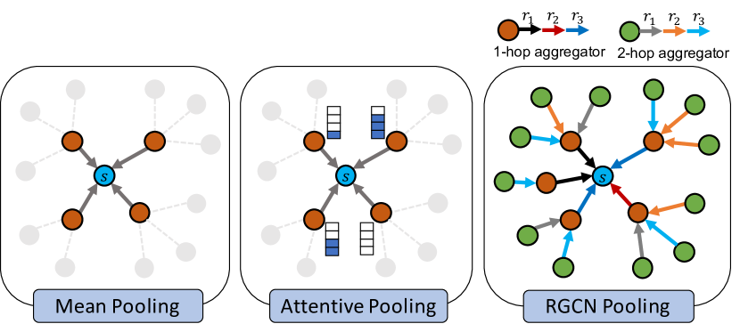
Figure 3: Comparison of neighborhood aggregators. The blue node corresponds to node $\mathrm{s}$, red nodes are 1-hop neighbors, and green nodes are 2-hop neighbors. Different colored edges are different relations. Mean and attentive pooling aggregators do not differentiate different relations and do not encode 2-hop neighbors, whereas RGCN aggregator can incorporate information from multi-relational and multi-hop neighbors.

3.2 Neighborhood Aggregators

In this section, we first introduce two simple aggregation functions: a mean pooling aggregator and an attentive pooling aggregator. These two simple aggregators only collect neighboring entities under the same relation $\mathrm{r}$. Then we introduce a more powerful aggregation function: a multi-relational aggregator. We depict comparison on aggregators in Fig. 3.

Mean Pooling Aggregator. The baseline aggregator simply takes the element-wise mean of representations in $\{\boldsymbol{e}_{\mathrm{o}}:\mathrm{o}\in\text{N}_{t}^{(\mathrm{s},\mathrm{r})}\}$, where $\text{N}_{t}^{(\mathrm{s},\mathrm{r})}$ is the set of objects that interacted with $\mathrm{s}$ under $\mathrm{r}$ at $t$. But the mean aggregator treats all neighboring objects equally, and thus ignores the different importance of each neighbor entity.

Attentive Pooling Aggregator. We define an attentive aggregator based on the additive attention introduced in (Bahdanau et al., 2015) to distinguish the important entities for $(\mathrm{s},\mathrm{r})$. The aggregate function is defined as $g(\text{N}_{t}^{(\mathrm{s},\mathrm{r})})=\sum_{\mathrm{o}\in\text{N}_{t}^{(\mathrm{s},\mathrm{r})}}\alpha_{\mathrm{o}}\boldsymbol{e}_{\mathrm{o}}$, where $\alpha_{\mathrm{o}}=\textrm{softmax}(\mathbf{v}^{\top}\tanh(\boldsymbol{W}(\boldsymbol{e}_{\mathrm{s}};\boldsymbol{e}_{\mathrm{r}};\boldsymbol{e}_{\mathrm{o}})))$. $\mathbf{v}\in\mathbb{R}^{d}$ and $\boldsymbol{W}\in\mathbb{R}^{d\times 3d}$ are trainable weight matrices. By adding the attention function of the subject and the relation, the weight can determine how relevant each object entity is to the subject and the relation.

Multi-Relational Graph (RGCN) Aggregator. We introduce a multi-relational graph aggregator from (Schlichtkrull et al., 2018). This is a general aggregator that can incorporate information from multi-relational and multi-hop neighbors. Formally, the aggregator is defined as follows:

$$g(\text{N}^{(\mathrm{s})}_{t})=\mathbf{h}_{s}^{(l+1)}=\sigma\Big{(}\sum_{\mathrm{r}\in R}\sum_{\mathrm{o}\in\text{N}_{t}^{(\mathrm{s},\mathrm{r})}}\frac{1}{c_{s}}\boldsymbol{W}_{r}^{(l)}\mathbf{h}_{\mathrm{o}}^{(l)}+\boldsymbol{W}_{0}^{(l)}\mathbf{h}_{s}^{(l)}\Big{)},$$ (8)

where initial hidden representations for each node ($\mathbf{h}_{o}^{(0)}$) are set to trainable embedding vectors ($\boldsymbol{e}_{\mathrm{o}}$) for each node and $c_{s}$ is a normalizing factor. Details are described in Section B of appendix.

Input: Observed graph sequence: $\{G_{1},...,G_{t}\}$, Number of events to sample at each step: $M$.

Output: An estimation of the conditional distribution $p(G_{t+\Delta t}|G_{:t})$.

1 $t^{\prime}\leftarrow t+1$

2 while $t^{\prime}\leq t+\Delta t$ do

3       Sample $M$ number of $\mathrm{s}~{}\sim p(\mathrm{s}|\hat{G}_{t+1:t^{\prime}-1},G_{:t})$ by equation (4).

4       Pick top-$k$ triples $\{(\mathrm{s}_{1},\mathrm{r}_{1},\mathrm{o}_{1},t^{\prime}),...,(\mathrm{s}_{k},\mathrm{r}_{k},\mathrm{o}_{k},t^{\prime})\}$ ranked by $p(\mathrm{s},\mathrm{r},\mathrm{o}|\hat{G}_{t+1:t^{\prime}-1},G_{:t})$.

5       ${\hat{G}}_{t^{\prime}}\leftarrow\{(\mathrm{s}_{1},\mathrm{r}_{1},\mathrm{o}_{1},t^{\prime}),...,(\mathrm{s}_{k},\mathrm{r}_{k},\mathrm{o}_{k},t^{\prime})\}$

6       $t^{\prime}\leftarrow t^{\prime}+1$

7Estimate the probability of each event $p(\mathrm{s},\mathrm{r},\mathrm{o}|\hat{G}_{t+1:t+\Delta t-1},G_{:t})$.

8 Estimate the joint distribution of all events $p(G_{t+\Delta t}|\hat{G}_{t+1:t+\Delta t-1},G_{:t})$ by equation (1).

return $p(G_{t+\Delta t}|\hat{G}_{t+1:t+\Delta t-1},G_{:t})$ as an estimation.

Algorithm 1 Learning algorithm of RE-Net

3.3 Parameter Learning and Inference

In this section, we discuss how RE-Net is trained and infers events over multiple time stamps.

Parameter Learning via Event Predictions. An object entity prediction given $(\mathrm{s},\mathrm{r})$ can be viewed as a multi-class classification task, where each class corresponds to each object entity. Similarly, relation prediction given $\mathrm{s}$ and subject entity prediction can be considered as a multi-class classification task. Here we omit the notations for preceding events for brevity. Thus, the loss function is as follows:

$$\mathcal{L}=-\sum_{(\mathrm{s},\mathrm{r},\mathrm{o},t)\in G}\log p(\mathrm{o}_{t}|\mathrm{s}_{t},\mathrm{r}_{t})+\lambda_{1}\log p(\mathrm{r}_{t}|\mathrm{s}_{t})+\lambda_{2}\log p(\mathrm{s}_{t}),$$ (9)

where $G$ is set of events, and $\lambda_{1}$ and $\lambda_{2}$ are importance parameters that control the importance of each loss term. $\lambda_{1}$ and $\lambda_{2}$ can be chosen depending on the task. If a task aims to predict $o$ given $(s,r)$, then we can give small values to $\lambda_{1}$ and $\lambda_{2}$.

Multi-step Inference over Time. RE-Net seeks to predict the forthcoming events based on the previous observations. Suppose that the current time is $t$ and we aim to predict events at time $t+\Delta t$ where $\Delta t>0$. Then the problem of multi-step inference can be formalized as inferring the conditional probability $p(G_{t+\Delta t}|G_{:t})$. The problem is nontrivial as we need to integrate over all $G_{t+1:t+\Delta t-1}$. To achieve efficient inference, we draw a sample of $G_{t+1:t+\Delta t-1}$, and estimate the conditional probability as follows:

$$p(G_{t+\Delta t}|G_{:t})$$

$$=\sum_{G_{t+1:t+\Delta t-1}}p(G_{t+\Delta t},G_{t+1:t+\Delta t-1}|G_{:t})$$

$$=\sum_{G_{t+1:t+\Delta t-1}}p(G_{t+\Delta t}|G_{:t+\Delta t-1})\cdots p(G_{t+1}|G_{:t})$$

$$=\mathbb{E}_{G_{t+1:t+\Delta t-1}|G_{:t}}[p(G_{t+\Delta t}|G_{:t+\Delta t-1})]$$

$$\simeq p(G_{t+\Delta t}|\hat{G}_{t+1:t+\Delta t-1},G_{:t}).$$

Intuitively, one starts with computing $p(G_{t+1}|G_{:t})$, and drawing a sample $\hat{G}_{t+1}$ from the conditional distribution. With this sample, one can further compute $p(G_{t+2}|\hat{G}_{t+1},G_{:t})$. By iteratively computing the conditional distribution for $G_{t^{\prime}}$ and drawing a sample from it, one can eventually estimate $p(G_{t+\Delta t}|G_{:t})$ as $p(G_{t+\Delta t}|\hat{G}_{t+1:t+\Delta t-1},G_{:t})$. Although we can improve the estimation by drawing multiple graph samples at each step, RE-Net already performs very well with a single sample, and thus we only draw one sample graph at each step for better efficiency. Based on the estimation of the conditional distribution, we can further predict events that are likely to form in the future. We summarize the detailed inference algorithm in Algorithm 1; we first sample $M$ number of $\mathrm{s}$ (line 1) and pick top-$k$ triples (line 1). Then we build a graph at time $t^{\prime}$ (line 1) to generate a graph. The time complexity of the algorithm is described in Section C of appendix.

4 Experiments

Table 1: Performance comparison on temporal link prediction (average metrics in % over 5 runs) on three event-based TKG datasets (ICEWS18, GDELT, and ICEWS14) and two public knowledge graphs (WIKI and YAGO). RE-Net achieves the best results.

Method		ICEWS18			GDELT			ICEWS14			WIKI			YAGO
		MRR	H@3	H@10	MRR	H@3	H@10	MRR	H@3	H@10	MRR	H@3	H@10	MRR	H@3	H@10
Static	DistMult	22.16	26.00	42.18	18.71	20.05	32.55	19.06	22.00	36.41	46.12	49.81	51.38	59.47	60.91	65.26
	R-GCN	23.19	25.34	36.48	23.31	24.94	34.36	26.31	30.43	45.34	37.57	39.66	41.90	41.30	44.44	52.68
	ConvE	36.85	39.92	50.54	35.56	39.45	49.16	40.46	43.33	54.75	47.55	49.78	49.42	62.66	63.36	65.57
	RotatE	23.10	27.61	38.72	22.33	23.89	32.29	29.56	32.92	42.68	48.67	49.74	49.88	64.09	64.67	66.16
Temporal	TA-DistMult	28.53	31.57	44.96	29.35	31.56	41.39	20.78	22.80	35.26	48.09	49.51	51.70	61.72	63.32	65.19
	HyTE	7.31	7.50	14.95	6.37	6.72	18.63	11.48	13.04	22.51	43.02	45.12	49.49	23.16	45.74	51.94
	dyngraph2vecAE	1.52	1.99	2.02	4.53	1.87	1.87	10.83	12.70	15.02	5.30	5.27	5.45	0.93	0.84	0.95
	tNodeEmbed	8.32	9.74	17.47	19.97	22.62	32.72	17.84	20.16	32.88	9.54	10.44	16.60	4.22	4.16	8.4
	EvolveRGCN	16.59	18.32	34.01	15.55	19.23	31.54	17.01	18.97	32.58	46.49	47.83	49.23	59.74	61.03	61.69
	Know-Evolve*	3.27	3.23	3.26	2.43	2.35	2.41	1.42	1.37	1.43	0.09	00.03	0.10	00.07	0	0.04
	Know-Evolve+MLP	9.29	9.62	17.18	22.78	25.49	35.41	22.89	26.68	38.57	12.64	14.33	21.57	6.19	6.59	11.48
	DyRep+MLP	9.86	10.66	18.66	23.94	27.88	36.58	24.61	28.87	39.34	11.60	12.74	21.65	5.87	6.54	11.98
	R-GCRN+MLP	35.12	38.26	50.49	37.29	41.08	51.88	36.77	40.15	52.33	47.71	48.14	49.66	53.89	56.06	61.19
	RE-Net w. mean agg.	40.70	43.27	53.65	38.35	42.13	52.52	43.79	47.34	57.47	51.13	51.37	53.01	65.10	65.24	67.34
	RE-Net w. attn agg.	40.96	44.08	54.32	38.54	42.25	52.85	43.94	47.85	57.91	51.25	52.54	53.12	65.13	65.54	67.87
	RE-Net	42.93	45.47	55.80	40.42	43.40	53.70	45.71	49.06	59.12	51.97	52.07	53.91	65.16	65.63	68.08

Evaluating the quality of generated graphs is non-trivial, especially for knowledge graphs (Theis et al., 2015). In our experiments, we evaluate the proposed method on a extrapolation link prediction task on TKGs. The task of predicting future links aims to predict unseen relationships with object entities given $(\mathrm{s},\mathrm{r},?,t)$ (or subject entities given $(?,\mathrm{r},\mathrm{o},t)$) at future time $t$, based on the past observed events in the TKG. Essentially, the task is a ranking problem over all the events $(\mathrm{s},\mathrm{r},?,t)$ (or $(?,\mathrm{r},\mathrm{o},t)$). RE-Net can approach this problem by computing the probability of each event in a distant future with the inference algorithm in Algorithm 1, and further rank all the events according to their probabilities. Note that we are only given a training set as ground truth at inference and we do not use any ground truth in the test set for the next time step predictions when performing multi-step inference. This is the main difference from previous work; they use previous ground truth in the test set.

We evaluate our proposed method on three benchmark tasks: (1) predicting future events on three event-based datasets; (2) predicting future facts on two knowledge graphs which include facts with time spans, and (3) studying ablation of our proposed method. Section 4.1 summarizes the datasets. In all these experiments, we perform predictions on time stamps that are not observed during training.

4.1 Experimental Setup

We compare the performance of our model against various traditional models for knowledge graphs, as well as some recent temporal reasoning models on five public datasets.

Datasets. We use five TKG datasets in our experiments: 1) three event-based TKGs: ICEWS18 (Boschee et al., 2015), ICEWS14 (Trivedi et al., 2017), and GDELT (Leetaru and Schrodt, 2013); and 2) two knowledge graphs where temporally associated facts have meta-facts as $(\mathrm{s},\mathrm{r},\mathrm{o},[t_{s},t_{e}])$ where $t_{s}$ is the starting time point and $t_{e}$ is the ending time point: WIKI (Leblay and Chekol, 2018) and YAGO (Mahdisoltani et al., 2014).

Evaluation Setting and Metrics. For each dataset except ICEWS14, we split it into three subsets, i.e., train(80%)/valid(10%)/test(10%), by time stamps. Thus, (time stamps of train) $<$ (time stamps of valid) $<$ (time stamps of test). We report a filtered version of Mean Reciprocal Ranks (MRR) and Hits$@3$/$10$. Similar to the definition of filtered setting in (Bordes et al., 2013), during evaluation, we remove all the valid triplets that appear in the train, valid, or test sets from the list of corrupted triplets.

Baselines. We compare our approach to baselines for static graphs and temporal graphs as follows:

(1) Static Methods. By ignoring the edge time stamps, we construct a static, cumulative graph for all the training events, and apply multi-relational graph representation learning methods including DistMult (Yang et al., 2015), R-GCN (Schlichtkrull et al., 2018), ConvE (Dettmers et al., 2018), and RotatE (Sun et al., 2019).

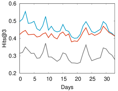
(a) ICEWS18

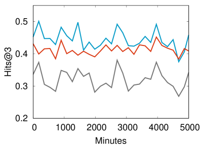
(b) GDELT

Figure 4: Performance of temporal link prediction over future timestamps with filtered Hits@3. RE-Net consistently outperforms the baselines.

(2) Temporal Reasoning Methods. We also compare state-of-the-art temporal reasoning methods for knowledge graphs, including Know-Evolve (Trivedi et al., 2017), TA-DistMult (García-Durán et al., 2018), and HyTE (Dasgupta et al., 2018). TA-DistMult and HyTE are for an interpolation task whereas we focus on an extrapolation task. To do this, we assign random values to temporal embeddings that are not observed during training. To see the effectiveness of our recurrent event encoder, we use encoders of previous work and our MLP decoder as baselines; we compare Know-Evolve, Dyrep (Trivedi et al., 2019), and GCRN (Seo et al., 2017) combined with our MLP decoder, called Know-Evolve+MLP, DyRep+MLP, and R-GCRN+MLP. The GCRN utilizes Graph Gonvolutional Network (Kipf and Welling, 2016). Instead, we use RGCN (Schlichtkrull et al., 2018) to deal with multi-relational graphs.

We also compare our method with dynamic methods on homogeneous graphs: dyngraph2vecAE (Goyal et al., 2019), tNodeEmbed (Singer et al., 2019), and EvolveRGCN (Pareja et al., 2020). These methods were proposed to predict interactions at future time on homogeneous graphs. Thus, we modified the methods to apply them on multi-relational graph.

(3) Variants of RE-Net. To evaluate the importance of different components of RE-Net, we varied our model in different ways: RE-Net w/o multi-step which does not update history during inference, RE-Net without the aggregator (RE-Net w/o agg.), RE-Net with a mean aggregator (RE-Net w. mean agg.), and RE-Net with an attentive aggregator (RE-Net w. attn agg.). RE-Net w/o agg. takes a zero vector instead of an aggregator. RE-Net w. GT denotes RE-Net with ground truth history.

Please refer to Section D of appendix for detailed experimental settings.

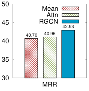
(a) RE-Net with different aggregators

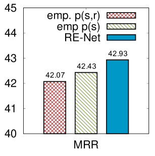
(b) Study of empirical $p(s)$ and $p(s,r)$

Figure 5: Performance study on model variations. We study the effects of (a) RE-Net with different aggregators, and (b) empirical $p(\mathrm{s})$ and $p(\mathrm{s},\mathrm{r})$.

4.2 Performance Comparison on TKGs.

We compare our proposed method with other baselines. The test results are obtained by averaged metrics (5 runs) over the entire test sets on datasets.

Results on Event-based TKGs. Table 1 summarizes results on all datasets. Our proposed RE-Net outperforms all other baselines on ICEWS18 and GDELT. Static methods underperform compared to our method since they do not consider temporal factors. Also, RE-Net outperforms all other temporal methods including TA-DistMult, HyTE, and dynamic methods on homogeneous graphs. Know-Evovle+MLP significantly improves Know-Evolve, which shows effectiveness of our MLP decoder. However, there is still a large gap from our model, which also indicates effectiveness of our recurrent event encoder. R-GCRN+MLP has a similar structure to ours in that it has a recurrent encoder and an RGCN aggregator but it lacks multi-step inference, global information, and the sophisticated modeling for the recurrent encoder. Thus, it underperforms compared to our method. More importantly, none of the prior temporal methods are capable of multi-step inference, while RE-Net can sequentially infer multi-step events (Details in Section 4.3).

Results on Public KGs. Previous results have demonstrated the effectiveness of RE-Net on event-based KGs. In Table 1 we compare RE-Net with other baselines on the Public KGs WIKI and YAGO. Our proposed RE-Net outperforms all other baselines on these datasets. In these datasets, baselines show better results than in the event-based TKGs. This is due to the characteristics of the datasets; they have facts that are valid within a time span. However, our proposed method consistently outperforms the static and temporal methods, which implies that RE-Net effectively infers new events using a powerful event encoder and an aggregator, and provides accurate prediction results.

Performance of Prediction over Time. Next, we further study performance of RE-Net over time. Figs. 4 shows the performance comparisons over different time stamps on the ICEWS18, GDELT, WIKI, and YAGO datasets with filtered Hits@3 metrics. RE-Net consistently outperforms baseline methods for all different time stamps. Performance of each method fluctuate since testing entities are different at each time step. We notice that with increasing time steps, the difference between RE-Net and ConvE gets smaller as shown in Fig. 4. This is expected since further future events are harder to predict. To estimate the joint probability distribution of events in a distant future, RE-Net needs to generate a long graph sequence. The quality of generated graphs deteriorates when RE-Net generates a long graph sequence.

Table 2: Ablation study on the ICEWS18 and GDELT datasets.

Method	ICEWS18			GDELT
	MRR	H@3	H@10	MRR	H@3	H@10
RE-Net w/o agg.	33.46	35.98	46.62	38.10	41.26	51.61
RE-Net w/o multi-step	40.05	42.60	52.92	38.72	42.52	52.78
RE-Net	42.93	45.47	55.80	40.42	43.40	53.70
RE-Net w. GT	44.33	46.83	57.27	41.80	45.71	56.03

4.3 Ablation Study

In this section, we study the effect of variations in RE-Net on the ICEWS18 dataset. We present the results in Tables 1, 2, and Fig. 5.

Different Aggregators. In Table 2, we observe that RE-Net w/o agg. hurts model quality, suggesting that introducing aggregators makes the model capable of dealing with concurrent events and improves performance. Table 1 and Fig. 5a show the performance of RE-Net with different aggregators. Among them, RGCN aggregator outperforms other aggregators. This aggregator has the advantage of exploring multi-relational neighbors. Also, RE-Net with an attentive aggregator shows better performance than RE-Net with a mean aggregator, which implies that giving different attention weights to each neighbor helps predictions.

Multi-step Inference. In Table 2, we observe that RE-Net outperforms RE-Net w/o multi-step. The latter one does not update history during inference; keeps its last history in the training set. So it is not affected by time stamps. Without the multi-step inference, the performance of RE-Net is decreased as is shown. Also we expect that RE-Net w. GT shows significant improvement when RE-Net uses ground truth of triples at the previous time step which are not allowed in our setup.

Empirical Probabilities. Here, we study the role of $p(\mathrm{s}_{t}|G_{t-m:t-1})$ and $p(\mathrm{r}_{t}|\mathrm{s},G_{t-m:t-1})$. We denote them as $p(\mathrm{s})$ and $p(\mathrm{r})$ for brevity. $p(\mathrm{s}_{t},\mathrm{r}_{t}|G_{t-m:t-1})$ (or simply $p(\mathrm{s},\mathrm{r})$) is equivalent to $p(\mathrm{s})p(\mathrm{r})$. In Fig 5b, emp. $p(\mathrm{s})$ (or $p_{e}(\mathrm{s})$) denotes a model with empirical $p(\mathrm{s})$, defined as $p_{e}(\mathrm{s})=$ (# of $\mathrm{s}$-related triples) / (total # of triples). emp. $p(\mathrm{s},\mathrm{r})$ (or $p_{e}(\mathrm{s},\mathrm{r})$) denotes a model with $p_{e}(\mathrm{s})$ and $p_{e}(\mathrm{r})$,defined as $p_{e}(\mathrm{r})=$ (# of $\mathrm{r}$-related triples) / (total # of triples). Thus, $p_{e}(\mathrm{s},\mathrm{r})=p_{e}(\mathrm{s})p_{e}(\mathrm{r})$. Note that RE-Net use a trained $p(\mathrm{s})$ and $p(\mathrm{r})$. The results show that the trained $p(\mathrm{s})$ and $p(\mathrm{r})$ help RE-Net for multi-step predictions. $p_{e}(\mathrm{s})$ underperforms RE-Net, and $p_{e}(\mathrm{s},\mathrm{r})=p_{e}(\mathrm{s})p_{e}(\mathrm{r})$ shows the worst performance, suggesting that training each part of the probability in equation (1) improves performance.

5 Related Work

Temporal KG Reasoning. There have been some recent attempts on incorporating temporal information in modeling dynamic knowledge graphs, broadly categorized into two settings - extrapolation (Trivedi et al., 2017) and interpolation (García-Durán et al., 2018; Leblay and Chekol, 2018; Dasgupta et al., 2018; Goel et al., 2020; Lacroix et al., 2020). For the former setting, Know-Evolve (Trivedi et al., 2017) models the occurrence of a fact as a temporal point process. For the latter setting, several embedding-based methods have been proposed (García-Durán et al., 2018; Leblay and Chekol, 2018; Dasgupta et al., 2018; Goel et al., 2020; Lacroix et al., 2020) to model time information. They embed the associate into a low dimensional space such as relation embeddings with RNN on the text of time (García-Durán et al., 2018), time embeddings (Leblay and Chekol, 2018), temporal hyperplanes (Leblay and Chekol, 2018), diachronic entity embedding (Goel et al., 2020), and tensor decomposition (Lacroix et al., 2020). However, these models cannot predict future events, as representations of unseen time stamps are unavailable.

Temporal Modeling on Homogeneous Graphs. There are attempts on predicting future links on homogeneous graphs (Pareja et al., 2020; Goyal et al., 2018, 2019; Zhou et al., 2018; Singer et al., 2019). Some of the methods try to incorporate and learn graphical structures to predict future links (Pareja et al., 2020; Zhou et al., 2018; Singer et al., 2019), while other methods predict by reconstructing an adjacency matrix by using an autoencoder (Goyal et al., 2018, 2019). These methods seek to predict on single-relational graphs, and are designed to predict future edges in one future step (i.e., for $t+1$). However, our work focuses on multi-relational knowledge graphs and aims for multi-step prediction.

Deep Autoregressive Models. Deep autoregressive models define joint probability distributions as a product of conditionals. DeepGMG (Li et al., 2018) and GraphRNN (You et al., 2018) are deep generative models of graphs and focus on generating static homogeneous graphs where there is only a single type of edge. In contrast to these studies, our work focuses on generating heterogeneous graphs, in which multiple types of edges exist, and thus our problem is more challenging. To the best of our knowledge, this is the first paper to formulate the structure inference (prediction) problem for temporal, multi-relational (knowledge) graphs in an autoregressive fashion.

6 Conclusion

To tackle the extrapolation problem, we proposed Recurrent Event Network (RE-Net) to model temporal, multi-relational, and concurrent interactions between entities. RE-Net defines the joint probability of all events, and thus is capable of inferring graphs in a sequential manner. The experiment revealed that RE-Net outperforms all the static and temporal methods and our extensive analysis shows its strength. Interesting future work includes developing a fast and efficient version of RE-Net, and modeling lasting events and performing inference on the long-lasting graph structures.

Appendix A Recurrent Neural Network

We define a recurrent event encoder based on RNN as follows:

$$\boldsymbol{h}_{t}(\mathrm{s},\mathrm{r})=\textrm{RNN}(g(\text{N}_{t}(\mathrm{s})),\boldsymbol{H}_{t},\boldsymbol{h}_{t-1}(\mathrm{s},\mathrm{r})).$$

We use Gated Recurrent Units (Cho et al., 2014) as RNN:

$$\boldsymbol{a}_{t} =[\boldsymbol{e}_{\mathrm{s}}:\boldsymbol{e}_{\mathrm{r}}:g(\text{N}_{t}(\mathrm{s})):\boldsymbol{H}_{t}]$$

$$\boldsymbol{z}_{t} =\sigma(\boldsymbol{W}_{z}\boldsymbol{a}_{t}+\boldsymbol{U}_{z}\boldsymbol{h}_{t-1})$$

$$\boldsymbol{r}_{t} =\sigma(\boldsymbol{W}_{r}\boldsymbol{a}_{t}+\boldsymbol{U}_{r}\boldsymbol{h}_{t-1})$$

$$\boldsymbol{h}_{t} =(1-\boldsymbol{z}_{t})\circ\boldsymbol{h}_{t-1}+\boldsymbol{z}_{t}\circ\tanh(\boldsymbol{W}_{h}\boldsymbol{a}_{t}+\boldsymbol{U}_{h}(\boldsymbol{r}_{t}\circ\boldsymbol{h}_{t-1})),$$

where $:$ is concatenation, $\sigma(\cdot)$ is an activation function, and $\circ$ is a Hadamard operator. The input is a concatenation of four vectors: subject embedding, object embedding, aggregation of neighborhood representations, and global information vector ($\boldsymbol{e}_{\mathrm{s}},\boldsymbol{e}_{\mathrm{r}},g(\text{N}_{t}(\mathrm{s})),\boldsymbol{H}_{t}$). $\boldsymbol{h}_{t}(s)$ and $\boldsymbol{H}_{t}$ are similarly defined. For $\boldsymbol{h}_{t}(s)$, a concatenation of subject embedding, aggregation of neighborhood representations, and global information vector ($\boldsymbol{e}_{\mathrm{s}},g(\text{N}_{t}(s)),\boldsymbol{H}_{t}$) is input. For $\boldsymbol{H}_{t}$, aggregation of the whole graph representations $g(G_{t})$ is input.

Appendix B Details of RGCN Aggregator

The RGCN aggregator is defined as follows:

$$g(\text{N}^{(\mathrm{s})}_{t})=\mathbf{h}_{s}^{(l+1)}=\sigma\Big{(}\sum_{\mathrm{r}\in R}\sum_{\mathrm{o}\in\text{N}_{t}^{(\mathrm{s},\mathrm{r})}}\frac{1}{c_{s}}\boldsymbol{W}_{r}^{(l)}\mathbf{h}_{\mathrm{o}}^{(l)}+\boldsymbol{W}_{0}^{(l)}\mathbf{h}_{s}^{(l)}\Big{)},$$ (10)

where initial hidden representations for each node ($\mathbf{h}_{o}^{(0)}$) are set to trainable embedding vectors ($\boldsymbol{e}_{\mathrm{o}}$) for each node and $c_{s}$ is a normalizing factor. Detailed

Basically, each relation can derive a local graph structure between entities, which further yield a message on each entity by aggregating information from neighbors, i.e., $\sum_{\mathrm{o}\in\text{N}_{t}^{(\mathrm{s},\mathrm{r})}}\allowbreak\frac{1}{c_{s}}\boldsymbol{W}_{r}^{(l)}\mathbf{h}_{\mathrm{o}}^{(l)}$. The overall message on each entity is further computed by aggregating all the relation-specific messages, i.e., $\sum_{\mathrm{r}\in R}\sum_{\mathrm{o}\in\text{N}_{t}^{(\mathrm{s},\mathrm{r})}}\allowbreak\frac{1}{c_{s}}\boldsymbol{W}_{r}^{(l)}\mathbf{h}_{\mathrm{o}}^{(l)}$. Finally, the aggregator $g(\text{N}^{(\mathrm{s})}_{t})$ is defined by combining both the overall message and information from past steps, i.e., $\boldsymbol{W}_{0}^{(l)}\mathbf{h}_{s}^{(l)}$.

To distinguish weights between different relations, we adopt independent weight matrices $\{\boldsymbol{W}_{\mathrm{r}}^{(l)}\}$ for each relation $\mathrm{r}$. Furthermore, the aggregator collects representations of multi-hop neighbors by introducing multiple layers of the neural network with each layer indexed by $l$. The number of layers determines the depth to which the node reaches to aggregate information from its local neighborhood.

The major issue of this aggregator is that the number of parameters grows rapidly with the number of relations. In practice, this can easily lead to overfitting on rare relations and models of very large size. Thus, we adopt the block-diagonal decomposition (Schlichtkrull et al., 2018), where each relation-specific weight matrix is decomposed into a block-diagonal by decomposing into low-dimensional matrices. $\boldsymbol{W}_{r}^{(l)}$ in equation (10) is defined as a block diagonal matrix, $\text{diag}(\mathbf{A}_{1r}^{(l)},...,\mathbf{A}_{Br}^{(l)})$ where $\mathbf{A}_{kr}^{(l)}\in\mathbb{R}^{(d^{(l+1)}/B)\times(d^{(l)}/B)}$ and $B$ is the number of basis matrices. The block decomposition reduces the number of parameters and helps prevent overfitting.

Appendix C Computational Complexity Analysis.

We analyze the time complexity of the graph generation process in Algorithm 1. Computing $p(\mathrm{s}_{t}|\allowbreak G_{t-m:t-1})$ (equation (4)) takes $O(|E|Lm)$, where $|E|$ is the maximum number of triples among $\{G_{t-m},...,G_{t-1}\}$, $L$ is the number of layers of aggregation, and $m$ is the number of the past time steps since we unroll $m$ time steps in RNN. From this probability, we sample $M$ number of subjects $\mathrm{s}$. Computing $p(\mathrm{s}_{t},\mathrm{r}_{t},\mathrm{o}_{t}|G_{t-m:t-1})$ in equation (1) takes $O(D^{L}m)$, where $D$ is the maximum degree of entities. To get probabilities of all possible triples given sampled subjects, it requires $O(M|R||O|D^{L}m)$ where $|R|$ is the total number of relations and $|O|$ is the total number of entities. Thus, the time complexity for generating one graph is $O(|E|Lm+M|R||O|(D^{L}m+\log k))$ where $k$ is the cutoff number for picking top-$k$ triples. The time complexity is linear to the number of entities and relations, and the number of sampled $\mathrm{s}$.

Table 3: Dataset Statistics.

Data	$N_{train}$	$N_{valid}$	$N_{test}$	$N_{ent}$	$N_{rel}$	Time gap
GDELT	1,734,399	238,765	305,241	7,691	240	15 mins
ICEWS18	373,018	45,995	49,545	23,033	256	24 hours
ICEWS14	323,895	-	341,409	12,498	260	24 hours
WIKI	539,286	67,538	63,110	12,554	24	1 year
YAGO	161,540	19,523	20,026	10,623	10	1 year

Appendix D Detailed Experimental Settings

Datasets. We use five datasets: 1) three event-based temporal knowledge graphs and 2) two knowledge graphs where temporally associated facts have meta-facts as $(\mathrm{s},\mathrm{r},\mathrm{o},[t_{s},t_{e}])$ where $t_{s}$ is the starting time point and $t_{e}$ is the ending time point. The first group of graphs includes Integrated Crisis Early Warning System (ICEWS18  (Boschee et al., 2015) and ICEWS14 (Trivedi et al., 2017)), and Global Database of Events, Language, and Tone (GDELT) (Leetaru and Schrodt, 2013). The second group of graphs includes WIKI (Leblay and Chekol, 2018) and YAGO (Mahdisoltani et al., 2014). Dataset statistics are described on Table 3, where $N_{train}$, $N_{valid}$, and $N_{test}$ are the numbers of train set, valid set, and test set, respectively. $N_{ent}$ and $N_{rel}$ are the numbers of entities and relations. The time gap represents time granularity between adjacent events.

ICEWS18 is collected from 1/1/2018 to 10/31/2018, ICEWS14 is from 1/1/2014 to 12/31/2014, and GDELT is from 1/1/2018 to 1/31/2018. The ICEWS14 is from (Trivedi et al., 2017). We didn’t use their version of the GDELT dataset since they didn’t release the dataset.

WIKI and YAGO datasets have temporally associated facts $(\mathrm{s},\mathrm{r},\mathrm{o},\allowbreak[t_{s},t_{e}])$. We preprocess the datasets such that each fact is converted to $\{(\mathrm{s},\mathrm{r},\mathrm{o},t_{s}),(\mathrm{s},\mathrm{r},\mathrm{o},t_{\mathrm{s}}+1_{t}),...,(\mathrm{s},\mathrm{r},\mathrm{o},t_{e})\}$ where $1_{t}$ is a unit time to ensure each fact has a sequence of events. Noisy events of early years are removed (before 1786 for WIKI and 1830 for YAGO).

The difference between the first group and the second group is that facts happen multiple times (even periodically) on the first group (event-based knowledge graphs) while facts last long time but are not likely to occur multiple times in the second group.

Model details of RE-Net. We use Gated Recurrent Units (Cho et al., 2014) as our recurrent event encoder, where the length of history is set as $m=10$ which means saving past 10 event sequences. If the events related to $\mathrm{s}$ are sparse, we check the previous time steps until we get $m$ previous time steps related to the entity $\mathrm{s}$. We pretrain the parameters related to equations 4 and 5 due to the large size of training graphs. We use a multi-relational aggregator to compute $\boldsymbol{H}_{t}$. The aggregator provides hidden representations for each node and we max-pool over all hidden representations to get $\boldsymbol{H}_{t}$. We apply teacher forcing for model training over historical data, i.e., we use the ground truth rather than the model’s own prediction as the input of the next time step during training. At inference time, RE-Net performs multi-step prediction across the time stamps in dev and test sets. In each time step, we sample 1000 $(=M)$ number of subjects and save top-1000 $(=k)$ triples to use them as a generated graph . We set the size of entity/relation embeddings to be 200 and embedding of unobserved embeddings are randomly initialized. We use two-layer RGCN in the RGCN aggregator with block dimension $2\times 2$. The model is trained by the Adam optimizer (Kingma and Ba, 2014). We set $\lambda_{1}$ to 0.1, the learning rate to $0.001$ and the weight decay rate to 0.00001. All experiments were done on GeForce GTX 1080 Ti.

Table 4: Performance comparisons with raw metrics. We observe our method outperforms all other methods.

Method		ICEWS18			GDELT			ICEWS14			WIKI			YAGO
		MRR	H@3	H@10	MRR	H@3	H@10	MRR	H@3	H@10	MRR	H@3	H@10	MRR	H@3	H@10
Static	DistMult	13.86	15.22	31.26	8.61	8.27	17.04	9.72	10.09	22.53	27.96	32.45	39.51	44.05	49.70	59.94
	R-GCN	15.05	16.49	29.00	12.17	12.37	20.63	15.03	16.12	31.47	13.96	15.75	22.05	27.43	31.24	44.75
	ConvE	22.56	25.41	41.67	18.43	19.57	32.25	21.64	23.16	38.37	26.41	30.36	39.41	41.31	47.10	59.67
	RotatE	11.63	12.31	28.03	3.62	2.26	8.37	9.79	9.37	22.24	26.08	31.63	38.51	42.08	46.77	59.39
Temporal	TA-DistMult	15.62	17.09	32.21	10.34	10.44	21.63	11.29	11.60	23.71	26.44	31.36	38.97	44.98	50.64	61.11
	HyTE	7.41	7.33	16.01	6.69	7.57	19.06	7.72	7.94	20.16	25.40	29.16	37.54	14.42	39.73	46.98
	dyngraph2vecAE	1.36	1.54	1.61	4.53	1.87	1.87	6.95	8.17	12.18	2.67	2.75	3.00	0.81	0.74	0.76
	tNodeEmbed	7.21	7.64	15.75	12.97	12.61	21.22	13.36	13.13	24.31	8.86	10.11	16.36	3.82	3.88	8.07
	EvolveRGCN	10.31	10.52	23.65	6.54	5.64	15.22	8.32	7.64	18.81	27.19	31.35	38.13	40.50	45.78	55.29
	Know-Evolve*	0.11	0.00	0.47	0.11	0.02	0.10	0.05	0.00	0.10	0.03	0	0.04	0.02	0	0.01
	Know-Evolve+MLP	7.41	7.87	14.76	15.88	15.69	22.28	16.81	18.63	29.20	10.54	13.08	20.21	5.23	5.63	10.23
	DyRep+MLP	7.82	7.73	16.33	16.25	16.45	23.86	17.54	19.87	30.34	10.41	12.06	20.93	4.98	5.54	10.19
	R-GCRN+MLP	23.46	26.62	41.96	18.63	19.80	32.42	21.39	23.60	38.96	28.68	31.44	38.58	43.71	48.53	56.98
	RE-Net w. mean agg.	25.45	29.27	44.31	19.03	20.20	33.32	22.73	25.47	41.48	30.19	32.94	40.57	46.33	52.49	61.21
	RE-Net w. attn agg.	25.76	29.56	44.86	19.35	20.42	33.55	23.18	25.98	41.95	30.25	30.12	40.86	46.56	52.56	61.35
	RE-Net	26.62	30.27	45.57	19.60	20.56	33.89	23.85	14.63	42.58	30.87	33.55	41.27	46.81	52.71	61.93

Experimental Settings for Baseline Methods. In this section, we provide detailed settings for baselines. We use implementations of DistMult. We implemented TA-DistMult based on the implementation of Distmult. For TA-DistMult, We use temporal tokens with the vocabulary of year, month and day on the ICEWS dataset and the vocabulary of year, month, day, hour and minute on the GDELT dataset. We use use a binary cross-entropy loss for DistMult and TA-DistMult. We validate the embedding size among 100 and 200. We set the batch size to 1024, margin to 1.0, negative sampling ratio to 1, and use the Adam optimizer.

We use the implementation of HyTE. We use every timestamp as a hyperplane. The embedding size is set to 128, the negative sampling ratio to 5, and margin to 1.0. We use time agnostic negative sampling (TANS) for entity prediction, and the Adam optimizer.

We use the codes for ConvE and use implementation by Deep Graph Library. Embedding sizes are 200 for both methods. We use 1 to all negative sampling for ConvE and use 10 negative sampling ratio for RGCN, and use the Adam optimizer for both methods. We use the codes for Know-Evolve. For Know-Evolve, we fix the issue in their codes. Issues are described in Section G. We follow their default settings.

We use the code for RotatE. The hidden layer/embedding size is set to 100, and batch size 256; other values follow the best values for the larger FB15K dataset configurations supplied by the author. The author reports filtered metrics only, so we added the implementation of the raw setting.

Experimental Settings for Dynamic Methods. We compare our method with dynamic methods on homogeneous graphs: dyngraph2vecAE (Goyal et al., 2019), tNodeEmbed (Singer et al., 2019), and EvolveGCN-O (Pareja et al., 2020). These methods were proposed to predict interactions at a future time on homogeneous graphs, while our proposed method is for predicting interactions on multi-relational graphs (or knowledge graphs). Furthermore, those methods predict links at one future time stamp, whereas our method seeks to predict interactions at multiple future time stamps. We modified some methods to apply them on multi-relational graphs as follows. We adopt R-GCN (Schlichtkrull et al., 2018) for EvolveGCN-O and call it EvolveRGCN. We convert knowledge graphs into homogeneous graphs for dyngraph2vecAE. The idea of this method is to reconstruct an adjacency matrix using an auto-encoder and regard it as a future adjacency matrix. If we keep relations, relation-specific adjacency matrices will be extremely sparse; the method learns to reconstruct near-zero adjacency matrices. tNodeEmbed is a temporal method on homogeneous graphs. To use this on multi-relational graphs, we first train entity embeddings with DistMult and set these as initial embeddings for entities in tNodeEmbed. Also we give entity embeddings as input to LSTM of tNodeEmbed. We concatenate output of LSTM and relation embeddings to predict objects. We did not modified other methods since it is not trivial to extend the methods.

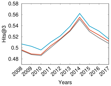
(a) WIKI

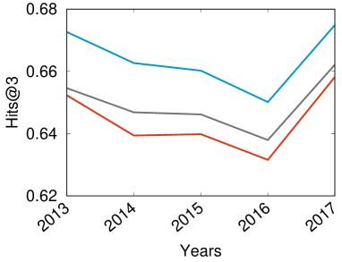
(b) YAGO

Figure 6: Performance of temporal link prediction over future timestamps with filtered Hits@3. RE-Net consistently outperforms the baselines.

Appendix E Additional Experiments

E.1 Results with Raw Metrics

Table 4 shows the performance comparison on ICEWS18, GDELT, ICEWS14 with raw settings. Our proposed RE-Net outperforms all other baselines.

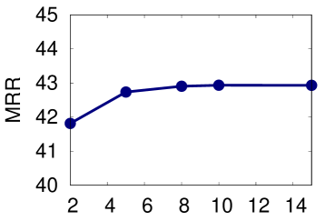
(a) Length of past history

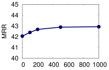
(b) Cutoff position $k$

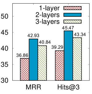
(c) # layers of RGCN

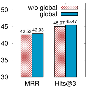
(d) Effect of global representations

Figure 7: Parameter sensitivity on RE-Net. We study the effects of (a) length of RNN history in event sequence encoder, and (b) cutoff position at inference time, (c) number of RGCN layers in neighborhood aggregation, and (d) effect of the global representation from a global graph structure.

E.2 Sensitivity Analysis

In this section, we study the parameter sensitivity of RE-Net including the length of history for the event encoder, cutoff position k for events to generate a graph, the number of layers of the RGCN aggregator, and effect of the global representation from a global graph structure. We report the performance change of RE-Net on the ICEWS18 dataset by varying the hyper-parameters (Figs. 7 and 7c).

Length of Past History in Recurrent Event Encoder. The recurrent event encoder takes the sequence of past interactions up to $m$ graph sequences or previous histories. Fig. 7a shows the performance with various lengths of past histories. When RE-Net uses longer histories, MRR is getting higher. However, the MRR is not likely to go higher when the length of history is 5 and over.

Cut-off Position $k$ at Inference. To generate a graph at each time, we cut off top-$k$ triples on ranking results. In Fig. 7b, when $k$ is 0, RE-Net does not generate graphs for estimating $p(G_{t+\Delta t}|G_{:t})$, i.e., RE-Net performs single-step predictions, and it shows the lowest result. When $k$ is larger, the performance is getting higher and it is saturated after 500. We notice that the conditional distribution $p(G_{t+\Delta t}|G_{:t})$ can be approximated by $p(G_{t+\Delta t}|\allowbreak\hat{G}_{t+1:t+\Delta t-1},G_{:t})$ by using a larger cutoff position.

Layers of RGCN Aggregator. The number of layers in the aggregator means the depth to which the node reaches. Fig. 7c shows the performance according to different numbers of layers of RGCN. 2-layered RGCN improves the performance considerably compared to 1-layered RGCN since 2-layered RGCN aggregates more information. However, RE-Net with 3-layered RGCN underperforms RE-Net with 2-layered RGCN. We conjecture that the bigger parameter space leads to overfitting.

Global Information. We further observe that representations from global graph structures help the predictions. Fig. 7d shows effectiveness of a representation of global graph structures. The improvement is marginal, but we consider that global representations at different time steps give distinct information beyond local graph structures.

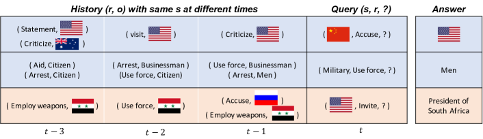
Figure 8: Case study of RE-Net’s predictions. RE-Net’s predictions depend on interaction histories. Interaction histories are categorized into three cases: (1) consistent interactions with an object, (2) a specific temporal pattern, and (3) irrelevant history. RE-Net achieves good performances on the first two cases, and poor performances on the third case.

Appendix F Case Study

In this section, we study RE-Net’s predictions. Its predictions depend on interaction histories. We categorize histories into three cases: (1) consistent interactions with an object, (2) a specific temporal pattern, and (3) irrelevant history (Fig. 8). RE-Net can learn (1) and (2) cases, so it achieves high performances. For the first case, RE-Net can predict the answer because it consistently interacts with an object. However, static methods are prone to predicting different entities which are observed under relation ”Accuse” in training set. The second case shows specific temporal patterns on relations: ( Arrest, $o$ ) $\rightarrow$ ( Use force, $o$ ). Without knowing this pattern, one method might predict “Businessman” instead of “Men”. RE-Net is able to learn these temporal patterns so it can predict the second case. Lastly, the third case shows irrelevant history to the answer and the history is not helpful to predictions. RE-Net fails to predict the third case.

Appendix G Implementation Issues of Know-Evolve

We found a problematic formulation in the Know-Evolve model and codes. The intensity function (equation 3 in (Trivedi et al., 2017)) is defined as $\lambda_{r}^{s,r}(t|\bar{t})=f(g_{r}^{s,r}(\bar{t}))(t-\bar{t})$, where $g(\cdot)$ is a score function, $t$ is current time, and $\bar{t}$ is the most recent time point when either subject or object entity was involved in an event. This intensity function is used in inference to rank entity candidates. However, they don’t consider concurrent event at the same time stamps, and thus $\bar{t}$ will become $t$ after one event. For example, we have events $e_{1}=(s,r,o_{1},t_{1}),e_{2}=(s,r,o_{2},t_{1})$. After $e_{1}$, $\bar{t}$ will become $t$ (subject $s$’s most recent time point), and thus the value of intensity function for $e_{2}$ will be 0. This is problematic in inference since if $t=\bar{t}$, then the intensity function will always be 0 regardless of entity candidates. In inference, all object candidates are ranked by the intensity function. But all intensity scores for all candidates will be 0 since $t=\bar{t}$, which means all candidates have the same 0 score. In their code, they give the highest ranks (first rank) for all entities including the ground truth object in this case. Thus, we fixed their code for a fair comparison; we give an average rank to entities who have the same scores.

References

- Bahdanau et al. (2015) Dzmitry Bahdanau, Kyunghyun Cho, and Yoshua Bengio. 2015. Neural machine translation by jointly learning to align and translate. CoRR, abs/1409.0473.
- Bordes et al. (2013) Antoine Bordes, Nicolas Usunier, Alberto García-Durán, Jason Weston, and Oksana Yakhnenko. 2013. Translating embeddings for modeling multi-relational data. In NIPS.
- Boschee et al. (2015) Elizabeth Boschee, Jennifer Lautenschlager, Sean O’Brien, Steve Shellman, James Starz, and Michael Ward. 2015. Icews coded event data. Harvard Dataverse, 12.
- Cho et al. (2014) Kyunghyun Cho, Bart van Merrienboer, Çaglar Gülçehre, Dzmitry Bahdanau, Fethi Bougares, Holger Schwenk, and Yoshua Bengio. 2014. Learning phrase representations using rnn encoder-decoder for statistical machine translation. In EMNLP.
- Dasgupta et al. (2018) Shib Sankar Dasgupta, Swayambhu Nath Ray, and Partha Talukdar. 2018. Hyte: Hyperplane-based temporally aware knowledge graph embedding. In EMNLP.
- Dettmers et al. (2018) Tim Dettmers, Pasquale Minervini, Pontus Stenetorp, and Sebastian Riedel. 2018. Convolutional 2d knowledge graph embeddings. In AAAI.
- García-Durán et al. (2018) Alberto García-Durán, Sebastijan Dumancic, and Mathias Niepert. 2018. Learning sequence encoders for temporal knowledge graph completion. In EMNLP.
- Goel et al. (2020) Rishab Goel, Seyed Mehran Kazemi, Marcus Brubaker, and Pascal Poupart. 2020. Diachronic embedding for temporal knowledge graph completion. In Thirty-Fourth AAAI Conference on Artificial Intelligence.
- Goyal et al. (2019) Palash Goyal, Sujit Rokka Chhetri, and Arquimedes Canedo. 2019. dyngraph2vec: Capturing network dynamics using dynamic graph representation learning. Knowledge-Based Systems, page 104816.
- Goyal et al. (2018) Palash Goyal, Nitin Kamra, Xinran He, and Yan Liu. 2018. Dyngem: Deep embedding method for dynamic graphs. arXiv preprint arXiv:1805.11273.
- Kazemi et al. (2019) Seyed Mehran Kazemi, Rishab Goel, Kshitij Jain, Ivan Kobyzev, Akshay Sethi, Peter Forsyth, and Pascal Poupart. 2019. Relational representation learning for dynamic (knowledge) graphs: A survey. arXiv preprint arXiv:1905.11485.
- Kingma and Ba (2014) Diederik P Kingma and Jimmy Ba. 2014. Adam: A method for stochastic optimization. arXiv preprint arXiv:1412.6980.
- Kipf and Welling (2016) Thomas N. Kipf and Max Welling. 2016. Semi-supervised classification with graph convolutional networks. CoRR, abs/1609.02907.
- Korkmaz et al. (2015) Gizem Korkmaz, Jose Cadena, Chris J Kuhlman, Achla Marathe, Anil Vullikanti, and Naren Ramakrishnan. 2015. Combining heterogeneous data sources for civil unrest forecasting. In Proceedings of the 2015 IEEE/ACM International Conference on Advances in Social Networks Analysis and Mining 2015, pages 258–265.
- Lacroix et al. (2020) Timothée Lacroix, Guillaume Obozinski, and Nicolas Usunier. 2020. Tensor decompositions for temporal knowledge base completion. In International Conference on Learning Representations.
- Leblay and Chekol (2018) Julien Leblay and Melisachew Wudage Chekol. 2018. Deriving validity time in knowledge graph. In Companion of the The Web Conference 2018 on The Web Conference 2018, pages 1771–1776. International World Wide Web Conferences Steering Committee.
- Leetaru and Schrodt (2013) Kalev Leetaru and Philip A Schrodt. 2013. Gdelt: Global data on events, location, and tone, 1979–2012. In ISA annual convention, volume 2, pages 1–49. Citeseer.
- Li et al. (2018) Yujia Li, Oriol Vinyals, Chris Dyer, Razvan Pascanu, and Peter Battaglia. 2018. Learning deep generative models of graphs. arXiv preprint arXiv:1803.03324.
- Mahdisoltani et al. (2014) Farzaneh Mahdisoltani, Joanna Asia Biega, and Fabian M. Suchanek. 2014. Yago3: A knowledge base from multilingual wikipedias. In CIDR.
- Morstatter et al. (2019) Fred Morstatter, Aram Galstyan, Gleb Satyukov, Daniel Benjamin, Andres Abeliuk, Mehrnoosh Mirtaheri, KSM Tozammel Hossain, Pedro Szekely, Emilio Ferrara, Akira Matsui, Mark Steyvers, Stephen Bennet, David Budescu, Mark Himmelstein, Michael Ward, Andreas Beger, Michele Catasta, Rok Sosic, Jure Leskovec, Pavel Atanasov, Regina Joseph, Rajiv Sethi, and Ali Abbas. 2019. Sage: A hybrid geopolitical event forecasting system. In Proceedings of the Twenty-Eighth International Joint Conference on Artificial Intelligence, IJCAI-19. International Joint Conferences on Artificial Intelligence Organization.
- Muthiah et al. (2015) Sathappan Muthiah, Bert Huang, Jaime Arredondo, David Mares, Lise Getoor, Graham Katz, and Naren Ramakrishnan. 2015. Planned protest modeling in news and social media. In AAAI.
- Pareja et al. (2020) Aldo Pareja, Giacomo Domeniconi, Jie Chen, Tengfei Ma, Toyotaro Suzumura, Hiroki Kanezashi, Tim Kaler, Tao B. Schardl, and Charles E. Leiserson. 2020. EvolveGCN: Evolving graph convolutional networks for dynamic graphs. In Proceedings of the Thirty-Fourth AAAI Conference on Artificial Intelligence.
- Phillips et al. (2017) Lawrence Phillips, Chase Dowling, Kyle Shaffer, Nathan Oken Hodas, and Svitlana Volkova. 2017. Using social media to predict the future: A systematic literature review. ArXiv, abs/1706.06134.
- Schlichtkrull et al. (2018) Michael Sejr Schlichtkrull, Thomas N. Kipf, Peter Bloem, Rianne van den Berg, Ivan Titov, and Max Welling. 2018. Modeling relational data with graph convolutional networks. In ESWC.
- Seo et al. (2017) Youngjoo Seo, Michaël Defferrard, Pierre Vandergheynst, and Xavier Bresson. 2017. Structured sequence modeling with graph convolutional recurrent networks. In ICONIP.
- Singer et al. (2019) Uriel Singer, Ido Guy, and Kira Radinsky. 2019. Node embedding over temporal graphs. arXiv preprint arXiv:1903.08889.
- Sun et al. (2019) Zhiqing Sun, Zhi-Hong Deng, Jian-Yun Nie, and Jian Tang. 2019. Rotate: Knowledge graph embedding by relational rotation in complex space. arXiv preprint arXiv:1902.10197.
- Theis et al. (2015) Lucas Theis, Aäron van den Oord, and Matthias Bethge. 2015. A note on the evaluation of generative models. arXiv preprint arXiv:1511.01844.
- Trivedi et al. (2017) Rakshit Trivedi, Hanjun Dai, Yichen Wang, and Le Song. 2017. Know-evolve: Deep temporal reasoning for dynamic knowledge graphs. In ICML.
- Trivedi et al. (2019) Rakshit Trivedi, Mehrdad Farajtabar, Prasenjeet Biswal, and Hongyuan Zha. 2019. Dyrep: Learning representations over dynamic graphs. In ICLR 2019.
- Yang et al. (2015) Bishan Yang, Wen tau Yih, Xiaodong He, Jianfeng Gao, and Li Deng. 2015. Embedding entities and relations for learning and inference in knowledge bases. CoRR, abs/1412.6575.
- You et al. (2018) Jiaxuan You, Rex Ying, Xiang Ren, William Hamilton, and Jure Leskovec. 2018. Graphrnn: Generating realistic graphs with deep auto-regressive models. In International Conference on Machine Learning, pages 5694–5703.
- Zhou et al. (2018) Lekui Zhou, Yang Yang, Xiang Ren, Fei Wu, and Yueting Zhuang. 2018. Dynamic network embedding by modeling triadic closure process. In Thirty-Second AAAI Conference on Artificial Intelligence.