Learning to Generate Synthetic Data via Compositing

Abstract

We present TERSE, a task-aware approach to synthetic data generation. Our framework employs a trainable synthesizer network that is optimized to produce meaningful training samples by assessing the strengths and weaknesses of a ‘target’ network. The synthesizer and target networks are trained in an adversarial manner wherein each network is updated with a goal to outdo the other. Additionally, we ensure the synthesizer generates realistic data by pairing it with a discriminator trained on real-world images. Further, to make the target classifier invariant to blending artefacts, we introduce these artefacts to background regions of the training images so the target does not over-fit to them.

We demonstrate the efficacy of our approach by applying it to different target networks including a classification network on AffNIST, and two object detection networks (SSD, Faster-RCNN) on different datasets. On the AffNIST benchmark, our approach is able to surpass the baseline results with just half the training examples. On the VOC person detection benchmark, we show improvements of up to $2.7\%$ as a result of our data augmentation. Similarly on the GMU detection benchmark, we report a performance boost of $3.5\%$ in mAP over the baseline method, outperforming the previous state of the art approaches by up to $7.5\%$ on specific categories.

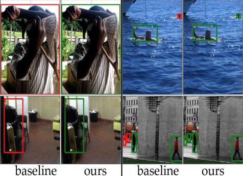
Figure 1: Comparison of object detection results using SSD. Baseline: trained on VOC data, Ours: trained on VOC and synthetic data generated using our approach. Green and red bounding boxes denote correct and missed detections respectively. SSD fine-tuned with our synthetic data shows improved performance on small, occluded and truncated person instances.

1 Introduction

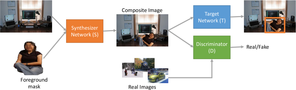
Figure 2: Our pipeline consists of three components: a synthesizer $\mathcal{S}$, the target network $\mathcal{T}$, and a natural image discriminator $\mathcal{D}$. $\mathcal{S}$ pastes an optimally transformed foreground into a background image to generate a synthetic composite image that can ‘fool’ $\mathcal{T}$ and $\mathcal{D}$. $\mathcal{T}$ is updated using the synthesized image to improve its accuracy. $\mathcal{D}$ provides feedback to $\mathcal{S}$ to improve realism of the synthetic image. $\mathcal{T}$ and $\mathcal{D}$ are updated with the synthesized data, in lock-step with $\mathcal{S}$.

Synthetic data generation is now increasingly utilized to overcome the burden of creating large supervised datasets for training deep neural networks. A broad range of data synthesis approaches have been proposed in literature, ranging from photo-realistic image rendering [22, 36, 49] and learning-based image synthesis [37, 41, 47] to methods for data augmentation that automate the process for generating new example images from an existing training set [9, 14, 15, 34]. Traditional approaches to data augmentation have exploited image transformations that preserve class labels [3, 47], while recent works [15, 34] use a more general set of image transformations, including even compositing images.

For the task of object detection, recent works have explored a compositing-based approach to data augmentation in which additional training images are generated by pasting cropped foreground objects on new backgrounds  [6, 7, 10]. The compositing approach, which is the basis for this work, has two main advantages in comparison to image synthesis: 1) the domain gap between the original and augmented image examples tends to be minimal (resulting primarily from blending artefacts) and 2) the method is broadly-applicable, as it can be applied to any image dataset with object annotations.

A limitation of prior approaches is that the process that generates synthetic data is decoupled from the process of training the target classifier. As a consequence, the data augmentation process may produce many examples which are of little value in improving performance of the target network. We posit that a synthetic data generation approach must generate data having three important characteristics. It must be a) task-aware: generate hard examples that help improve target network performance, b) efficient: generate fewer and meaningful data samples, and c) realistic: generate realistic examples that help minimize domain gaps and improve generalization.

We achieve these goals by developing a novel approach to data synthesis called TERSE, short for Task-aware Efficient Realistic Synthesis of Examples. We set up a 3-way competition among the synthesizer, target and discriminator networks. The synthesizer is tasked with generating composite images by combining a given background with an optimally transformed foreground, such that it can fool the target network as shown in Figure 2. The goal of the target network is to correctly classify/detect all instances of foreground object in the composite images. The synthesizer and target networks are updated iteratively, in a lock-step. We additionally introduce a real image discriminator to ensure the composite images generated by the synthesizer conform to the real image distribution. Enforcing realism prevents the model from generating artificial examples which are unlikely to occur in real images, thereby improving the generalization of the target network.

A key challenge with all composition-based methods is the sensitivity of trained models to blending artefacts. The target and discriminator networks can easily learn to latch on to the blending artefacts, thereby rendering the data generation process ineffective. To address these issues with blending, Dwibedi et al. [7] employed $5$ different blending methods so that the target network does not over-fit to a particular blending artefact. We propose an alternate solution to this problem by synthesizing examples that contain similar blending artefacts in the background. The artefacts are generated by pasting foreground shaped cutouts in the background images. This makes the target network insensitive to any blending artefacts around foreground objects, since the same artefacts are present in the background images as well.

We apply our synthesis pipeline to demonstrate improvements on tasks including digit classification on the AffNIST dataset [46], object localization using SSD [29] on Pascal VOC [8], and instance detection using Faster RCNN [35] on GMU Kitchen [11] dataset. We demonstrate that our approach is a) efficient: we achieve similar performance to baseline classifiers using less than $50\%$ data (Sec. 4.1), b) task-aware: networks trained on our data achieve up to $2.7\%$ improvement for person detection (Sec. 4.2) and $3.5\%$ increase in mAP over all classes on the GMU kitchen dataset over baseline (Sec. 4.3). We also show that our approach produces $>$2X hard positives compared to state-of-the-art [6, 7] for person detection. Our paper makes the following contributions:

• We present a novel image synthesizer network that learns to create composites specifically to fool a target network. We show that the synthesizer is effective at producing hard examples to improve the target network.

• We propose a strategy to make the target network invariant to artefacts in the synthesized images, by generating additional hallucinated artefacts in the background images.

• We demonstrate applicability of our framework to image classification, object detection, and instance detection.

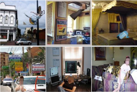
Figure 3: Using a discriminator improves the realism of generated images. (Top) Composite images generated without discriminator in the loop. (Bottom) Composite images generate with discriminator.

2 Related Work

To the best of our knowledge, ours is the first approach to generate synthetic data by compositing images in a task-aware fashion. Prior work on synthetic data generation can be organized into three groups: 1) Image composition, 2) Adversarial generation, and 3) Rendering.

Image Composition: Our work is inspired by recent cut and paste approaches [6, 7, 10] to synthesize positive examples for object detection tasks. The advantage of these approaches comes from generating novel and diverse juxtapositions of foregrounds and backgrounds that can substantially increase the available training data. The starting point for our work is the approach of Dwibedi et al. [7], who were first to demonstrate empirical boosts in performance through the cut and paste procedure. Their approach uses random sampling to decide the placement of foreground patches on background images. However, it can produce unrealistic compositions which limits generalization performance as shown by [6]. To help with generalization, prior works [6, 10] exploited contextual cues [4, 30, 31] to guide the placement of foreground patches and improve the realism of the generated examples. Our data generator network implicitly encodes contextual cues which is used to generate realistic positive examples, guided by the discriminator. We therefore avoid the need to construct explicit models of context [4, 6]. Other works have used image compositing to improve image synthesis [45], multi-target tracking [20], and pose tracking [38]. However, unlike our approach, none of these prior works optimize for the target network while generating synthetic data.

Adversarial learning: Adversarial learning has emerged as a powerful framework for tasks such as image synthesis, generative sampling, synthetic data generation etc. [2, 5, 26, 44] We employ an adversarial learning paradigm to train our synthesizer, target, and discriminator networks. Previous works such as A-Fast-RCNN  [51] and the adversarial spatial transformer (ST-GAN) [26] have also employed adversarial learning for data generation. The A-Fast-RCNN method uses adversarial spatial dropout to simulate occlusions and an adversarial spatial transformer network to simulate object deformations, but does not generate new training samples. The ST-GAN approach uses a generative model to synthesize realistic composite images, but does not optimize for a target network.

Rendering: Recent works [1, 16, 36, 41, 48, 52] have used simulation engines to render synthetic images to augment training data. Such approaches allow fine-grained control over the scale, pose, and spatial positions of foreground objects, thereby alleviating the need for manual annotations. A key problem of rendering based approaches is the domain difference between synthetic and real data. Typically, domain adaptation algorithms (e.g. [41]) are necessary to bridge this gap. However, we avoid this problem by compositing images only using real data.

Hard example mining: Previous works have shown the importance of hard examples for training robust models [19, 27, 39, 53, 54, 29]. However, most of these approaches mine existing training data to identify hard examples and are bound by limitations of the training set. Unlike our approach, these methods do not generate new examples. Recently, [18, 55] proposed data augmentation for generating transformations that yields additional pseudo-negative training examples. In contrast, we generate hard positive examples.

3 TERSE Data Synthesis

Our approach for generating hard training examples through image composition requires as input a background image, $b$, and a segmented foreground object mask, $m$, from the object classes of interest. The learning problem is formulated as a 3-way competition among the synthesizer $\mathcal{S}$, the target $\mathcal{T}$, and the discriminator $\mathcal{D}$. We optimize $\mathcal{S}$ to produce composite images that can fool both $\mathcal{T}$ and $\mathcal{D}$. $\mathcal{T}$ is updated with the goal to optimize its target loss function, while $\mathcal{D}$ continues to improve its classification accuracy. The resulting synthetic images are both realistic and constitute hard examples for $\mathcal{T}$. The following sections describe our data synthesis pipeline and end-to-end training process in more detail.

3.1 Synthesizer Network

The synthesizer operates on the inputs $b$ and $m$ and outputs a transformation function, $A$. This transformation is applied to the foreground mask to produce a composite synthetic image, $f=b\oplus A(m)$, where $\oplus$ denotes the alpha-blending [26] operation. In this work, we restrict $A$ to the set of 2D affine transformations (parameterized by a $6-$ dimensional feature vector), but the approach can trivially be extended to other classes of image transformations. $b,f,A$ are then fed to a Spatial Transformer module [17] which produces the composite image $f$ (Figure  2). The composite image is fed to the discriminator and target networks with the goal of fooling both of them. The synthesizer is trained in lockstep with the target and discriminator as described in the following sections.

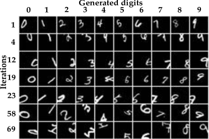
Figure 4: Data generated by our approach over multiple iterations for the AffNIST experiment (Section 4.1). As training progresses (top to bottom) the synthesized examples become more complex, from single modes of failure of the target network to multiple modes at later stages.

Blending Artefacts: In order to paste foreground regions into backgrounds, we use the standard alpha-blending method described in [17]. One practical challenge, as discussed in [7], is that the target model can learn to exploit any artefacts introduced by the blending function, as these will always be associated with positive examples, thereby harming the generalization of the classifier. Multiple blending strategies are used in [7] to discourage the target model from exploiting the blending artefacts. However, a target model with sufficient capacity could still manage to over-fit on all of the different blending functions that were used. Moreover, it is challenging to generate a large number of candidate blending functions due to the need to ensure differentiability in end-to-end learning.

We propose a simple and effective strategy to address this problem. We explicitly introduce blending artefacts into the background regions of synthesized images (see Fig. 5). To implement this strategy, we (i) randomly choose a foreground mask from our training set, (ii) copy background region shaped like this mask from one image, and (iii) paste it onto the background region in another image using the same blending function used by $\mathcal{S}$. As a consequence of this process, the presence of a composited region in an image no longer has any discriminative value, as the region could consist of either foreground or background pixels. This simple strategy makes both the discriminator and the target model invariant to any blending artefacts.

3.2 Target Network

The target model is a neural network trained for specific objectives such as image classification, object detection, semantic segmentation, regression, etc. Typically, we first train the target $\mathcal{T}$ with a labeled dataset to obtain a baseline level of performance. This pre-trained baseline model $\mathcal{T}$ is then fine-tuned in lockstep with $\mathcal{S}$ and $\mathcal{D}$. Our synthetic data generation framework is applicable to a wide range of target networks. Here we derive the loss for the two common cases of image classification and object detection.

Image Classification: For the task of image classification, the target loss function $\mathcal{L}_{\mathcal{T}}$ is the standard cross-entropy loss over the training dataset.

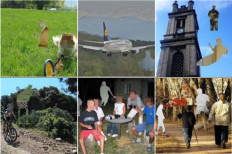
Figure 5: Examples of blending artefacts pasted into background regions of training images in order to remove any discriminative cues associated with compositing. A random foreground-shaped cut-out from a different background image is pasted on the background regions of the given image. Images from COCO (top row) and VOC (bottom row) are shown.

Object Detection: For detection frameworks such as SSD [29] and faster-RCNN [35], for each bounding-box proposal, the target network outputs (a) probability distribution $p=(p^{0},\cdots,p^{L})$ over the $L+1$ classes in the dataset (including background), (b) bounding-box regression offsets $r\in\mathbb{R}^{4}$. While SSD uses fixed anchor-boxes, faster-RCNN uses CNN based proposals for bounding boxes. The ground truth class labels and bounding box offsets for each proposal are denoted by $c$ and $v$, respectively. Anchor boxes with an Intersection-over-Union (IoU) overlap greater than $0.5$ with the ground-truth bounding box are labeled with the class of the bounding box, and the rest are assigned to the background class. The object detector target $\mathcal{T}$ is trained to optimize the following loss function:

$$\centering\mathcal{L}_{\mathcal{T}}(p,c,r,v)=\underbrace{-\log(p^{c})}_{\text{classification objective}}+\underbrace{\lambda[c>0]L_{loc}(r,v)}_{\text{localization objective}}\@add@centering$$ (1)

where, $L_{loc}$ is the smooth $L_{1}$ loss function defined in [12]. The Iverson bracket indicator function $[c>0]$ evaluates to $1$ for $c>0$, i.e. for non-background classes and $0$ otherwise. In other words, only the non-background anchor boxes contribute to the localization objective.

3.3 Natural Image Discriminator

An unconstrained cut-paste approach to data augmentation can produce non-realistic composite images (see for example Fig. 3). Synthetic data generated in such a way can still potentially improve the target network as shown by Dwibedi et al. [7]. However, as others [4, 30, 31] have shown, generating contextually salient and realistic synthetic data can help the target network to learn more efficiently and generalize more effectively to real world tasks.

Instead of learning specific context and affordance models, as employed in aforementioned works, we adopt an adversarial training approach and feed the output of the synthesizer to a discriminator network as negative examples. The discriminator also receives positive examples in the form of real-world images. It acts as a binary classifier that differentiates between real images $r$ and composite images $f$. For an image $I$, the discriminator outputs $\mathcal{D}(I)$, i.e. the probability of $I$ being a real image. $\mathcal{D}$ is trained to maximize the following objective:

$$\mathcal{L}_{\mathcal{D}}=\mathbb{E}_{r}\log(\mathcal{D}(r))+\mathbb{E}_{f}\log(1-\mathcal{D}(f)).$$ (2)

As illustrated in Figure 3, the discriminator helps the synthesizer to produce more natural looking images.

3.4 Training Details

The three networks, $\mathcal{S}$, $\mathcal{T}$, and $\mathcal{D}$, are trained according to the following objective function:

$$\mathcal{L}_{\mathcal{S},\mathcal{T},\mathcal{D}}=\max_{\mathcal{S}}\min_{\mathcal{T}}\mathcal{L}_{\mathcal{T}}+\min_{\mathcal{S}}\max_{\mathcal{D}}\mathcal{L}_{\mathcal{D}}$$ (3)

For a given training batch, parameters of $\mathcal{S}$ are updated while keeping parameters of $\mathcal{T}$ and $\mathcal{D}$ fixed. Similarly, parameters of $\mathcal{T}$ and $\mathcal{D}$ are updated by keeping parameters of $\mathcal{S}$ fixed. $\mathcal{S}$ can be seen as an adversary to both $\mathcal{T}$ and $\mathcal{D}$.

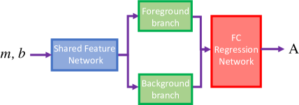
Figure 6: Synthesizer Architecture

Synthesizer Architecture. Our synthesizer network (Figure 6) consists of (i) a shared low-level feature extraction backbone that performs identical feature extraction on foreground masks $m$ and background images $b$, (ii) and parallel branches for mid-level feature extraction on $m,b$, and (iii) a fully-connected regression network that takes as input the concatenation of mid-level features of $m,b$ and outputs a $6-$dimensional feature vector representing the affine transformation parameters. For the AffNIST experiments, we use a $2-$ layer network as the backbone. For experiments on Pascal VOC and GMU datasets, we use the VGG-16 [42] network up to Conv-5. The mid-level feature branches each consist of $2$ bottlenecks, with one convolutional layer, followed by ReLU and BatchNorm layers. The regression network consists of $2$ convolutional and $2$ fully connected layers.

Synthesizer hyper parameters. We use Adam [21] optimizer with a learning rate of $1e-3$ for experiments on the AffNIST dataset and $1e-4$ for all other experiments. We set the weight decay to $0.0005$ in all of our results.

Target fine-tuning hyper parameters. For the AffNIST benchmark, the target classifier is finetuned using the SGD optimizer with a learning rate of $1e-2$, a momentum of $0.9$ and weight decay of $0.0005$. For person detection on VOC, the SSD is finetuned using the Adam optimizer with a learning rate of $1e-5$, and weight decay of $0.0005$. For experiments on the GMU dataset, the faster-RCNN model is finetuned using the SGD optimizer with a learning rate of $1e-3$, weight decay of $0.0001$ and momentum of $0.9$.

4 Experiments & Results

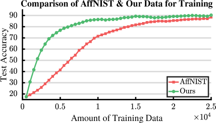
Figure 7: Performance of MNIST classifier on AffNIST test data when progressively augmented with (i) AffNIST training data (red), (ii) our synthetic images (green). Our approaches achieves baseline accuracy ($\approx 90\%$) with less than half the data ($12K$ samples vs $25K$ samples). Note that even with $5K$ samples we reach an accuracy of $\approx 80\%$, compared to baseline accuracy of $\approx 40\%$.

Table 1: Our approach achieves better classification accuracy compared to previous pseudo-negative data synthesis approaches on AffNIST dataset. Numbers are reported from the respective papers.

Method	DCGAN[32]	WGAN-GP[13]	ICN[18]	WINN[25]	ITN[55]	Ours
Error (%)	2.78	2.76	2.97	2.56	1.52	0.99

We now present qualitative and quantitative results to demonstrate the efficacy of our data synthesis approach.

4.1 Experiments on AffNIST Data

We show the efficiency of data generated using our approach on AffNIST [46] hand-written character dataset. It is generated by transforming MNIST [24] digits by randomly sampled affine transformations. For generating synthetic images with our framework, we apply affine transformations on MNIST digits and paste them onto black background images.

Target Architecture: The target classification model is a neural network consisting of two $5\times 5$ convolutional layers with $10$ and $20$ output channels, respectively. Each layer uses ReLU activation, followed by a dropout layer. The output features are then processed by two fully-connected layers with output sizes of $50$ and $10$, respectively.

We conducted two experiments with AffNIST dataset: Efficient Data Generation: The baseline classifier is trained on MNIST. The AffNIST model is fine-tuned by incrementally adding samples undergoing random affine transformation as described in [46]. Similarly, results from our method incrementally improves the classifier using composite images generated by $\mathcal{S}$.

Figure 1 shows the performance of the target model on the AffNIST test set by progressively increasing the size of training set. When trained on MNIST dataset alone, the target model has a classification accuracy of $~{}17\%$ on the AffNIST test set. We iteratively fine-tune the MNIST model from this point by augmenting the training set with $500$ images either from the AffNIST training set (red curve) or from the synthetic images generated by $\mathcal{S}$ (green curve). Note that our approach achieves baseline accuracy with less than half the data. In addition, as shown in Figure 1, using only $5K$ examples, our method improves accuracy from $40\%$ to $80\%$. Qualitative results in Figure 4 shows the progression of examples generated by $\mathcal{S}$. As training progresses, our approach generates increasingly hard examples in a variety of modes.

Improvement in Accuracy: In Table 1, we compare our approach with recent methods [55, 32, 13, 25, 18] that generate synthetic data to improve accuracy on AffNIST data. For the result in Table 1, we use $55000$, $5000$, $10000$ split for training, validation and testing as in [55] along with the same classifier architecture. We outperform hard negative generation approaches [55, 25, 18] by achieving a low error rate of $0.99\%$. Please find more details in the supplementary.

4.2 Experiments on Pascal VOC Data

We demonstrate improved results using our approach for person detection on the Pascal VOC dataset [8], using the SSD$-300$ network [29]. We use ground-truth person segmentations and bounding box annotations to recover instance masks from VOC 2007 and 2012 training and validation sets as foreground. Background images were obtained from the COCO dataset [28]. We do an initial clean up of those annotations since we find that for about $10\%$ of the images, the annotated segmentations and bounding-boxes do not agree. For evaluation we augment the VOC 2007 and 2012 training dataset with our synthetic images, and report mAP for detection on VOC 2007 test set for all experiments.

Figure 8: Comparison of our approach with Cut-Paste-Learn [7] and Context-Data-Augmentation [6], on the fraction of hard positives generated for the person class.

Baseline [29]			AP0.5 $\rightarrow$ $78.93$		AP0.8 $\rightarrow$ $29.52$
Column No.	1	2	3	4	5	6
Ann. Cleanup		✓	✓	✓	✓	✓
Dropout			✓	✓	✓	✓
Blending				✓	✓	✓
$1:1$ Ratio					✓	✓
Discriminator						✓
AP0.5	$79.02$	$79.13$	$79.02$	$79.34$	$79.61$	$79.53$
AP0.8	$29.64$	$30.72$	$30.80$	$31.25$	$31.96$	$32.22$

Table 2: Ablation Studies. We show the effect of design choices on the performance of our approach. Significant improvements are observed by introducing blending artefacts in background regions (col. 4) and maintaining a $1:1$ ratio between real and synthetic images (col 5) during training. Adding a discriminator provides additional boost at AP_0.8.

Dataset	coca cola	coffee mate	honey bunches	hunt’s sauce	mahatma rice	nature v1	nature v2	palmolive orange	pop secret	pringles bbq	red bull	mAP
Baseline faster-RCNN	$81.9$	$95.3$	$92.0$	$87.3$	$86.5$	$96.8$	$88.9$	$80.5$	$92.3$	$88.9$	$58.6$	$86.3$
Cut-Paste-Learn [7]	$\mathbf{88.5}$	$95.5$	$\mathbf{94.1}$	$88.1$	$\mathbf{90.3}$	$\mathbf{97.2}$	$91.8$	$80.1$	$94.0$	$\mathbf{92.2}$	$65.4$	$88.8$
Ours	$86.9$	$\mathbf{95.9}$	$93.9$	$\mathbf{90.2}$	$90.0$	$96.6$	$\mathbf{92.0}$	$\mathbf{87.6}$	$\mathbf{94.9}$	$90.9$	$\mathbf{69.2}$	$\mathbf{89.8}$

Table 3: Comparison of our approach with the baseline Faster-RCNN and [7] on the GMU Kitchen Dataset. Our approach improves overall mAP and outperforms other approaches in most classes.

4.2.1 Comparison with Previous Cut-Paste Methods

We compare our results with the performance of the baseline SSD network after fine-tuning it with the data generated by recent approaches from [6, 7]. We use the publicly available software from authors of [6, 7] to generate the same amount of synthetic data that we use in our experiments. To ensure a fair comparison, we use the same foreground masks and background images with added blending artifacts for the generation of synthetic data. We report detailed results over multiple IoU thresholds in Table 4, and some qualitative results in Figure 1.

As observed in [6], we note that adding data generated from [7] to training leads to a drop in performance. We also noticed that adding data generated by [6] also leads to a drop in SSD performance. In contrast, our method improves SSD performance by $2.7\%$ at AP_0.8.

Quality of Synthetic Data: We develop another metric to evaluate the quality of synthetic data for the task of person detection. A hardness metric is defined as $1-p$, where $p$ is the probability of the synthetic composite image containing a person, according to the baseline SSD. We argue that if the baseline network is easily able to detect the person in a composite image, then it is an easy example and may not boost the network’s performance when added to the training set. A similar metric has been proposed by previous works  [19, 40, 51, 54] for evaluating the quality of real data.

In Figure 8, we compare the hardness of data generated by our approach to to that of [6, 7]. The X-axis denotes the SSD confidence and the Y-axis captures fraction of samples generated. We generate the same amount of data with all methods and take an average over multiple experiment runs to produce this result. As shown in Figure 8, we generate significantly harder examples than  [6, 7]. Please find more qualitative examples and experiments in the supplementary material.

4.2.2 Ablation Studies

IoU	Baseline	[7]	[6]	Ours no-$\mathcal{D}$	Ours +$\mathcal{D}$
$0.5$	$78.93$	$76.65$	$76.81$	$\mathbf{79.61}$ ($\mathbf{+0.68}$)	$79.53$ ($+0.60$)
$0.6$	$69.61$	$66.88$	$66.91$	$70.39$ ($+0.78$)	$\mathbf{70.67}$ ($\mathbf{+1.06}$)
$0.7$	$52.97$	$52.12$	$50.21$	$53.71$ ($+0.74$)	$\mathbf{54.50}$ ($\mathbf{+1.53}$)
$0.8$	$29.54$	$28.82$	$28.14$	$31.96$ ($+2.44$)	$\mathbf{32.22}$ ($\mathbf{+2.68}$)

Table 4: Results on VOC 2007 test data for person detection. Our augmentation improves the baseline over different IoU thresholds by $~{}2.7\%$ at an IoU of $0.8$.

Table 2 studies the effect of various parameters on the performance of an SSD network fine-tuned on our data. In particular, we study the effect of (i) excluding noisy foreground segmentation annotations during generation, (ii) using dropout in the synthesizer, (iii) adding blending artifacts in the background, (iv) fine-tuning with real and synthetic data, and (v) adding the discriminator. Our performance metric is mAP at an IoU threshold of $0.5$. While we note progressive improvements in our performance with each addition, we see a slight drop in performance after the addition of the discriminator. We investigate this further in Table 4, and note that adding the discriminator improves our performance on all IoU thresholds higher $>0.5$, allowing us to predict bounding boxes which are much better aligned with the ground truth boxes.

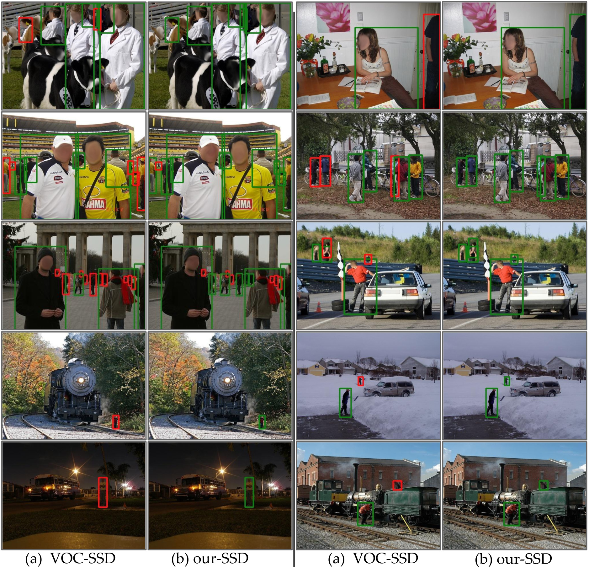
Figure 9: Qualitative results for VOC 2007 test set before and after training SSD with our synthesized data. Green and red boxes show correct and missed detections, respectively. Note that synthetic data helps improve the SSD performance on severely occluded and small instances.

4.3 Experiments on GMU Data

Lastly, we apply our data synthesis framework to improve the Faster-RCNN [35] for instance detection. We compare our approach with baseline Faster-RCNN and the method of [7] on the GMU Kitchen Dataset [11].

The GMU Kitchen Dataset comprises $11$ classes and has 3-fold train/test splits as reported in [7]. We use foregrounds from the Big Berkeley Instance Recognition (BigBIRD) [43] dataset and backgrounds from the UW Scenes dataset [23].

Table 3 reports per class accuracy and mean average precision on the GMU test set. Our approach out-performs baseline Faster-RCNN and [7] by $3.5\%$ and $1\%$ in mAP, respectively. Interestingly, we improve accuracy of some categories such as ’palmolive-orange’ by up to $7.5\%$.

5 Conclusion

The recent success of deep learning has been fueled by supervised training requiring human annotations. Large training sets are essential for improving performance under challenging real world environments, but are difficult, expensive and time-consuming to obtain. Synthetic data generation offers promising new avenues to augment training sets to improve the accuracy of deep neural networks.

In this paper, we introduced the concept of task-aware synthetic data generation to improve the performance of a target network. Our approach trains a synthesizer to generate efficient and useful synthetic samples, which helps to improve the performance of the target network. The target network provides feedback to the synthesizer, to generate meaningful training samples. We proposed a novel approach to make the target model invariant to blending artefacts by adding similar artefacts on background regions of training images. We showed that our approach is efficient, requiring less number of samples as compared to random data augmentations to reach a certain accuracy. In addition, we show a $2.7\%$ improvement in the state-of-art person detection using SSD. Thus, we believe that we have improved the state-of-art in synthetic data generation tailored to improve deep learning techniques.

Our work opens up several avenues for future research. Our synthesizer network outputs affine transformation parameters, but can be easily extended to output additional learnable photometric transformations to the foreground masks and non-linear deformations. We showed composition using a foreground and background image, but compositing multiple images can offer further augmentations. While we showed augmentations in 2D using 2D cut-outs, our work can be extended to paste rendered 3D models into 2D images. Our approach can also be extended to other target networks such as regression and segmentation networks. Future work includes explicitly adding a diversity metric to data synthesis to further improve its efficiency.

6 Acknowledgements

We wish to thank Kris Kitani for valuable discussions on this topic.

Supplementary Material: Learning to Generate Synthetic Data via Compositing

Appendix A Implementation Details

Our pipeline is implemented in python using the PyTorch deep-learning library. In the following subsections, we furnish relevant empirical details for our experiments on the different datasets in the manuscript.

A.1 Experiments on AffNIST data

In our experiments on the AffNIST benchmark, our synthesizer network generates affine transformations which are applied to MNIST images. These transformed images are then used to augment the MNIST training set and the performance of a handwritten digit classifier network trained on the augmented dataset is compared to an equivalent classifier trained on MNIST + AffNIST images. In the rest of the section, we give details about our experimental settings.

Data Pre-processing. For the AffNIST benchmark, our synthesizer network uses foreground masks from the MNIST training dataset. We pad the original $28\times 28$ MNIST images by $6$ black pixels on all sides to enlarge them to a $40\times 40$ resolution. This is done to ensure that images generated by our synthesizer have the same size as the AffNIST images which also have a spatial resolution of $40\times 40$ pixels.

Architecture of the Synthesizer Network. The synthesizer network takes as input a foreground image from the MNIST dataset and outputs a $6-$dimensional vector representing the affine parameters, namely the (i) angle of rotation, (ii) translation along the X$-$axis, (iii) translation along the Y$-$axis, (iv) shear, (v) scale along the X$-$axis, and (vi) scale along the Y$-$axis. We clamp these parameters to the same range used to generate AffNIST dataset. These parameters are used to define an affine transformation matrix which is fed to a Spatial Transformer module [17] alongside the foreground mask. The Spatial Transformer module applies the transformation to the foreground mask and returns the synthesized image. We attach the pytorch model dump for the synthesizer below.

⬇

1Features(

2 (BackBone): Sequential(

3 (0): C2d(1, 10, ksz=(5, 5), st=(1, 1))

4 (1): MaxPool2d(ksz=(3, 3), st=(2, 2))

5 (2): BN2d(10, eps=1e-05, mmntm=0.1)

6 (3): ReLU(inplace)

7 (4): Dropout2d(p=0.5)

8 )

9 (FgBranch): Sequential(

10 (0): C2d(10, 20, ksz=(3, 3), st=(1, 1))

11 (1): ReLU(inplace)

12 (2): BN2d(20, eps=1e-05, mmntm=0.1)

13 (3): Dropout2d(p=0.5)

14 (4): C2d(20, 20, ksz=(3, 3), st=(1, 1))

15 (5): ReLU(inplace)

16 (6): BN2d(20, eps=1e-05, mmntm=0.1)

17 (7): Dropout2d(p=0.5)

18 )

19)

20RegressionFC(

21 (features): Sequential(

22 (0): C2d(40, 20, ksz=(3, 3), st=(1, 1))

23 (1): ReLU(inplace)

24 (2): BN2d(20, eps=1e-05, mmntm=0.1)

25 (3): Dropout2d(p=0.5)

26 (4): C2d(20, 20, ksz=(3, 3), st=(1, 1))

27 (5): ReLU(inplace)

28 (6): BN2d(20, eps=1e-05, mmntm=0.1)

29 (7): Dropout2d(p=0.5)

30 )

31 (regressor): Sequential(

32 (0): Linear(in_f=1620, out_f=50, bias=True)

33 (1): ReLU(inplace)

34 (2): BatchNorm1d(50, eps=1e-05, mmntm=0.1)

35 (3): Dropout(p=0.5)

36 (4): Linear(in_f=50, out_f=20, bias=True)

37 (5): ReLU(inplace)

38 (6): BatchNorm1d(20, eps=1e-05, mmntm=0.1)

39 (7): Dropout(p=0.5)

40 (8): Linear(in_f=20, out_f=6, bias=True)

41 )

42)

The acronyms used in the pytorch model dump are described in Table. 5.

Acronym	Meaning
C2d	Conv2d
BN2d	BatchNorm2d
ksz	kernel_size
st	stride
pdng	padding
LReLU	LeakyReLU
neg_slp	negative_slope
InstNrm2D	InstanceNorm2d
mmntm	momentum
in_f	in_features
out_f	out_features

Table 5: Acronyms used within PyTorch model dumps.

Architecture of the Target Classifier. For our experiments in Figure. 7, we use a target model with two convolutional layers followed by a dropout layer, and two linear layers. The pytorch model dump is attached below.

⬇

1MNISTClassifier(

2 (0): C2d(1, 10, ksz=(5, 5), st=(1, 1))

3 (1): ReLU(inplace)

4 (2): C2d(10, 20, ksz=(5, 5), st=(1, 1))

5 (3): ReLU(inplace)

6 (4): Dropout2d(p=0.5)

7 (5): Linear(in_f=980, out_f=50, bias=True)

8 (6): ReLU(inplace)

9 (7): Linear(in_f=50, out_f=10, bias=True)

10)

For our experiments in Table. 1, we use the following architecture from [55], where Swish denotes the swish activation function from [33].

⬇

1MNISTClassifierDeep(

2 (0): C2d(1, 64, ksz=(5, 5), st=(2, 2))

3 (1): BN2d(64, eps=1e-05, mmntm=0.1)

4 (2): Swish(inplace)

5 (3): C2d(64, 64, ksz=(5, 5), st=(2, 2))

6 (4): BN2d(64, eps=1e-05, mmntm=0.1)

7 (5): Swish(inplace)

8 (6): C2d(64, 64, ksz=(5, 5), st=(2, 2))

9 (7): BN2d(64, eps=1e-05, mmntm=0.1)

10 (8): Swish(inplace)

11 (9): C2d(64, 64, ksz=(5, 5), st=(2, 2))

12 (10): BN2d(64, eps=1e-05, mmntm=0.1)

13 (11): Swish(inplace)

14 (12): Linear(in_f=576, out_f=50, bias=True)

15 (13): Swish(inplace)

16 (14): Linear(in_f=50, out_f=10, bias=True)

17)

Training the Synthesizer Network. We use the ADAM optimizer with a batch-size of $1024$ and a fixed learning rate of $10^{-3}$. Xavier initialization is used with a gain of 0.4 to initialize the network weights. The synthesizer is trained in lock-step with the target model: we alternately update the synthesizer and target models. The weights of the target model are fixed during the synthesizer training. The synthesizer is trained until we find $500$ hard examples per class. A synthesized image is said to be a hard example if $p-p^{*}>0.05$ where $p*$ is the probability of it belonging to the ground truth class, and $p$ is the maximum probability over the other classes estimated by the target model. We maintain a cache of hard examples seen during the synthesizer training and use this cache for training dataset augmentation. We observed from our experiments that the number of epochs required to generated 500 images per class increases over sleep cycles as the target model became stronger.

Training the Target Network. The original training dataset consists of MNIST training images. After each phase of synthesizer network training we augment the training dataset with all images from the cache of hard examples and train the target network for $30$ epochs. The augmented dataset is used to fine-tune the classifier network. For fine-tuning, we use SGD optimizer with a batch-size of 64, $10^{-2}$ learning rate and a momentum of $0.5$. For our experiments in Table. $1$, we reduce the learning rate to $10^{-3}$ after $100$ iterations of training the synthesizer and target networks.

A.2 Experiments on Pascal VOC data

In our experiments on the Pascal VOC person detection benchmark, we additionally employ a natural versus synthetic image discriminator to encourage the synthetic images to appear realistic. We use the SSD$-300$ pipeline from [29] as the target model.

Data Pre-processing. We resize all synthetic images to $300\times 300$ pixels to be consistent with the SSD$-300$ training protocol. Background images for generating synthetic data are drawn from the COCO dataset, and foreground masks come from the VOC 2007 and 2012 trainval datasets. VOC datasets contain instance segmentation masks for a subset of trainval images. We use the ground truth segmentation masks and bounding box annotations to recover additional instance segmentation masks. We noticed that for about $10\%$ images the segmentation and bounding box detections do not agree, therefore we visually inspected the instance masks generated and filtered out erroneous ones. Figure 10 shows some images from the VOC dataset where the segmentation and bounding box annotations disagree, resulting in erroneous instance masks.

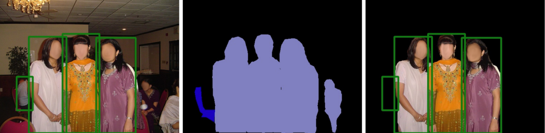
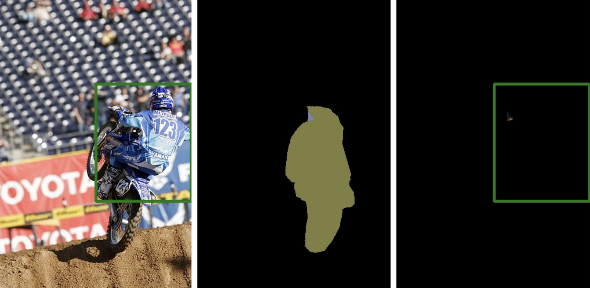
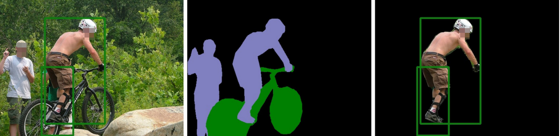
Figure 10: Disagreements between segmentation and detection annotations in the VOC dataset. Column $1$ shows ground truth bounding boxes overlaid on images. Column $2$ shows segmentation annotations. Column $3$ shows generated instance masks: each green box corresponds to one instance.

The foreground segmentations are centered and normalized such that $\max($height, width$)$ of the segmentation bounding-box occupies at least $0.7$ of the corresponding image dimension. We randomly pair background images with foreground instances while training the synthesizer network and during synthetic data generation.

Architecture of the Synthesizer Network. The synthesizer architecture is similar to the one used for AffNIST experiments with two enhancements: (i) we use the fully convolutional part of the the VGG$-16$ [42] network as the backbone, and (ii) we have an additional mid-level feature extraction subnetwork for the background image. This is described in the following model dump.

⬇

1Features(

2 (BackBone): Sequential(

3 (0): C2d(3, 64, ksz=(3, 3), pdng=(1, 1))

4 (1): BN2d(64, eps=1e-05, mmntm=0.1)

5 (2): ReLU(inplace)

6 (3): C2d(64, 64, ksz=(3, 3), pdng=(1, 1))

7 (4): BN2d(64, eps=1e-05, mmntm=0.1)

8 (5): ReLU(inplace)

9 (6): MaxPool2d(ksz=2, st=2)

10 (7): C2d(64, 128, ksz=(3, 3), pdng=(1, 1))

11 (8): BN2d(128, eps=1e-05, mmntm=0.1)

12 (9): ReLU(inplace)

13 (10): C2d(128, 128, ksz=(3, 3), pdng=(1, 1))

14 (11): BN2d(128, eps=1e-05, mmntm=0.1)

15 (12): ReLU(inplace)

16 (13): MaxPool2d(ksz=2, st=2)

17 (14): C2d(128, 256, ksz=(3, 3), pdng=(1, 1))

18 (15): BN2d(256, eps=1e-05, mmntm=0.1)

19 (16): ReLU(inplace)

20 (17): C2d(256, 256, ksz=(3, 3), pdng=(1, 1))

21 (18): BN2d(256, eps=1e-05, mmntm=0.1)

22 (19): ReLU(inplace)

23 (20): C2d(256, 256, ksz=(3, 3), pdng=(1, 1))

24 (21): BN2d(256, eps=1e-05, mmntm=0.1)

25 (22): ReLU(inplace)

26 (23): MaxPool2d(ksz=2, st=2)

27 (24): C2d(256, 512, ksz=(3, 3), pdng=(1, 1))

28 (25): BN2d(512, eps=1e-05, mmntm=0.1)

29 (26): ReLU(inplace)

30 (27): C2d(512, 512, ksz=(3, 3), pdng=(1, 1))

31 (28): BN2d(512, eps=1e-05, mmntm=0.1)

32 (29): ReLU(inplace)

33 (30): C2d(512, 512, ksz=(3, 3), pdng=(1, 1))

34 (31): BN2d(512, eps=1e-05, mmntm=0.1)

35 (32): ReLU(inplace)

36 (33): MaxPool2d(ksz=2, st=2)

37 )

38 (FgBranch): Sequential(

39 (0): C2d(512, 256, ksz=(3, 3), st=(1, 1))

40 (1): BN2d(256, eps=1e-05, mmntm=0.1)

41 (2): ReLU(inplace)

42 (3): C2d(256, 256, ksz=(3, 3), st=(1, 1))

43 (4): BN2d(256, eps=1e-05, mmntm=0.1)

44 (5): ReLU(inplace)

45 (6): C2d(256, 20, ksz=(3, 3), st=(1, 1))

46 )

47 (BgBranch): Sequential(

48 (0): C2d(512, 256, ksz=(3, 3), st=(1, 1))

49 (1): BN2d(256, eps=1e-05, mmntm=0.1)

50 (2): ReLU(inplace)

51 (3): C2d(256, 256, ksz=(3, 3), st=(1, 1))

52 (4): BN2d(256, eps=1e-05, mmntm=0.1)

53 (5): ReLU(inplace)

54 (6): C2d(256, 20, ksz=(3, 3), st=(1, 1))

55 )

56)

57RegressionFC(

58 (features): Sequential(

59 (0): C2d(40, 64, ksz=(5, 5), pdng=(2, 2))

60 (1): ReLU(inplace)

61 (2): BN2d(64, eps=1e-05, mmntm=0.1)

62 (3): C2d(64, 64, ksz=(5, 5), pdng=(2, 2))

63 (4): ReLU(inplace)

64 (5): BN2d(64, eps=1e-05, mmntm=0.1)

65 )

66 (regressor): Sequential(

67 (0): Linear(in_f=64, out_f=128, bias=True)

68 (1): ReLU(inplace)

69 (2): BatchNorm1d(128, eps=1e-05, mmntm=0.1)

70 (3): Linear(in_f=128, out_f=128, bias=True)

71 (4): ReLU(inplace)

72 (5): BatchNorm1d(128, eps=1e-05, mmntm=0.1)

73 (6): Linear(in_f=128, out_f=6, bias=True)

74 )

75)

Architecture of the Discriminator. Our discriminator is based on the discriminator architecture from [50].

⬇

1Discriminator(

2 (0): Sequential(

3 (0): C2d(3, 64, ksz=(4, 4), st=(2, 2), pdng=(2, 2))

4 (1): LReLU(neg_slp=0.2, inplace)

5 )

6 (1): Sequential(

7 (0): C2d(64, 128, ksz=(4, 4), st=(2, 2), pdng=(2, 2))

8 (1): InstNrm2D(128, eps=1e-05, mmntm=0.1, affine=False, track_running_stats=False)

9 (2): LReLU(neg_slp=0.2, inplace)

10 )

11 (2): Sequential(

12 (0): C2d(128, 256, ksz=(4, 4), st=(2, 2), pdng=(2, 2))

13 (1): InstNrm2D(256, eps=1e-05, mmntm=0.1, affine=False, track_running_stats=False)

14 (2): LReLU(neg_slp=0.2, inplace)

15 )

16 (3): Sequential(

17 (0): C2d(256, 512, ksz=(4, 4), st=(1, 1), pdng=(2, 2))

18 (1): InstNrm2D(512, eps=1e-05, mmntm=0.1, affine=False, track_running_stats=False)

19 (2): LReLU(neg_slp=0.2, inplace)

20 )

21 (4): Sequential(

22 (0): C2d(512, 1, ksz=(4, 4), st=(1, 1), pdng=(2, 2))

23 )

24 (5): AvgPool2d(ksz=3, st=2, pdng=[1, 1])

25)

Training the Synthesizer, Discriminator and Target Networks. The synthesizer is trained in lock-step with the discriminator and the target models: the discriminator and target model weights are fixed and the synthesizer is trained for $1000$ batches. The synthesizer is then used to generate synthetic images: we do a forward pass on $100$ batches of randomly paired foreground and background images and pick composite images which have a target estimated probability of less than $0.5$. These hard examples are added to the training dataset. The weights of the synthesizer network are then fixed and the discriminator and target models are trained for $3$ epochs over the training set. This cycle is repeated $5$ times.

The VGG-16 backbone of the synthesizer is initialized with an ImageNet pretrained model. The synthesizer is trained using the ADAM optimizer with a batch-size of $16$ and a fixed learning rate of $1e-4$ is used. The weights of the discriminator are randomly initialized to a Normal distribution with a variance of $0.02$. The discriminator is trained using the ADAM optimizer with a batch size of $16$ and a fixed learning rate of $1e-4$ is used. We initialize the SSD model with the final weights from [29]. The SSD model is trained using the SGD optimizer, a fixed learning rate of $1e-5$, momentum of $0.9$ and a weight decay of $0.0005$.

Custom Spatial Transformer. The image resizing during data pre-processing step and the spatial-transformer module both involve bilinear interpolation which introduces quantization artefacts near the segmentations mask edges. To deal with these artefacts we customize the Spatial Transformer implementation. More specifically, we remove these artefacts by subtracting a scalar($\mu=1-10^{-7}$) from the segmentation masks and applying ReLU non-linearity. The result is normalized back to a binary image. Gaussian blur is applied to the resulting mask for smooth transition near edges before applying alpha blending.

A.3 Experiments on GMU Kitchen data

Our experiments on the GMU data use the same synthesizer architecture and training strategy as described in Section. A.2 with one change: we do not use the discriminator in these experiments. We did not see noticeable improvements in performance with the addition of the discriminator in these experiments.

Appendix B Qualitative Results

Qualitative results follow on the next page.

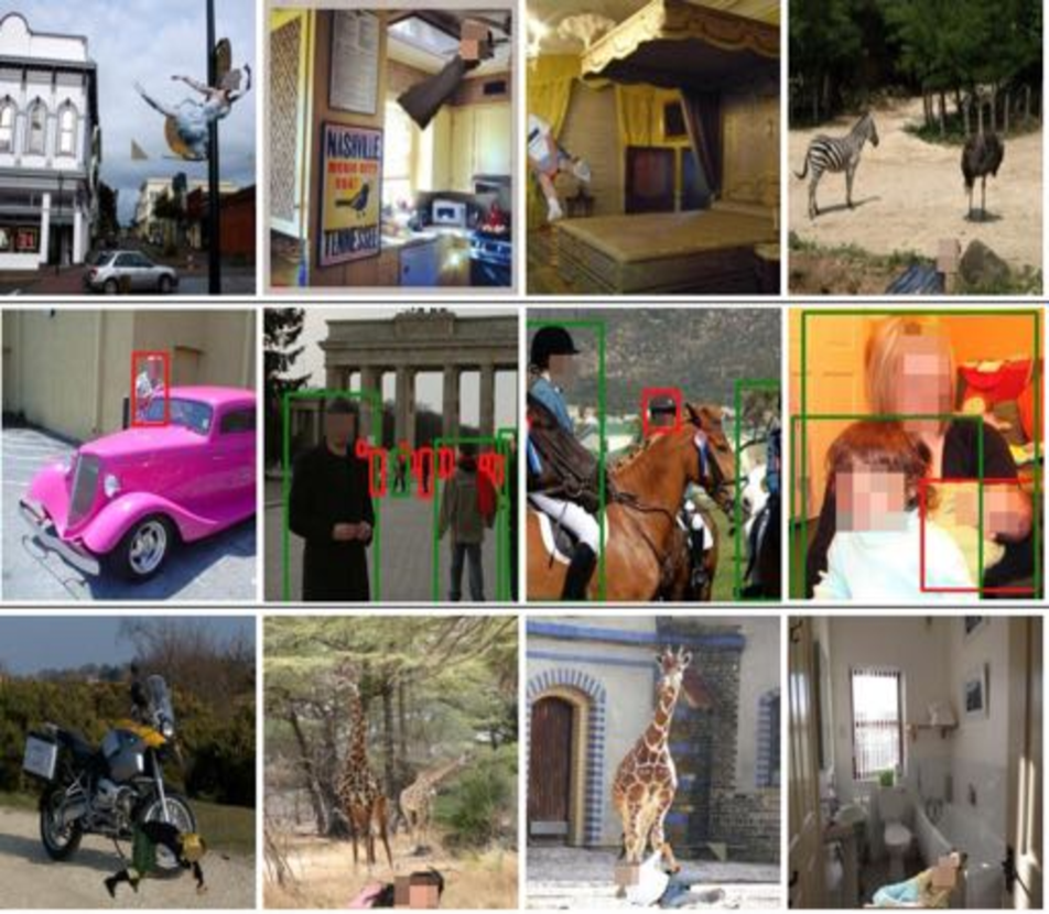
Figure 11: Qualitative results for Synthetic Data Generation. Row-1: Here we show the synthetic images generated by our synthesizer based on feedback from the baseline SSD trained on the VOC 2007-2012 dataset. These images evoke misclassifications from the baseline SSD primarily because they present human instances in unforeseen/unrealistic circumstances. Row-2: SSD failures on VOC 2007 test images after finetuning the baseline SSD with composite images such as those shown in Row-1. We notice the the three failure cases are a) person instances at small scales, b) horizontal pose, and c) severe occlusion. Row-3: Synthetic images generated by our synthesizer after feedback from the finetuned SSD. We notice that our synthesizer now generates small scales, horizontal pose and severely truncated instances.

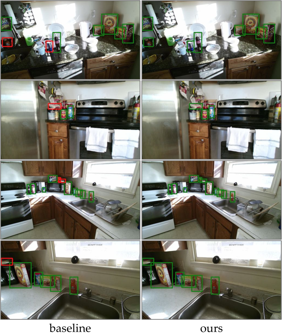
Figure 12: Qualitative improvements on the GMU Kitchen benchmark. Green and red bounding boxes denote correct and missing detections respectively.

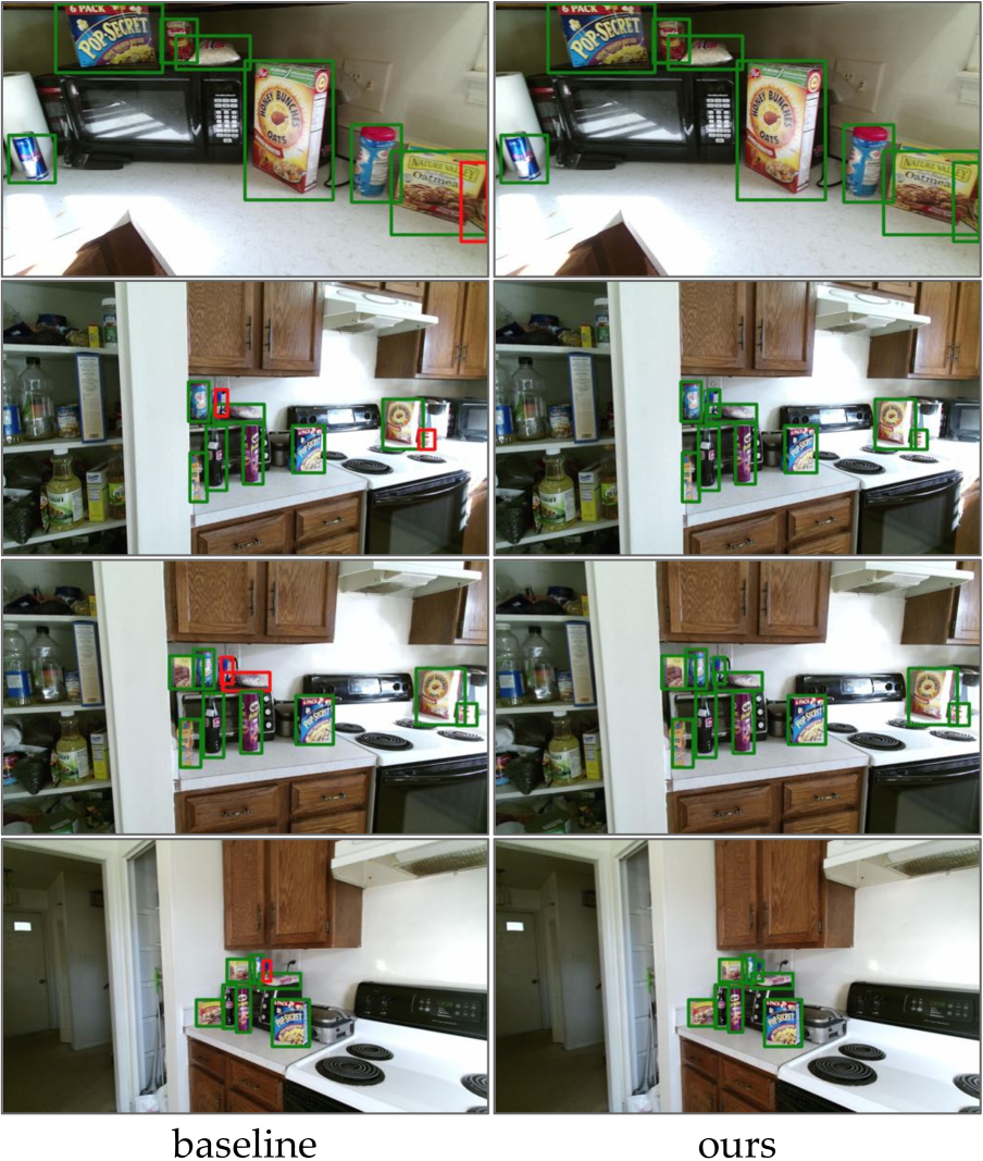
Figure 13: More qualitative improvements on the GMU Kitchen benchmark. Green and red bounding boxes denote correct and missing detections respectively.

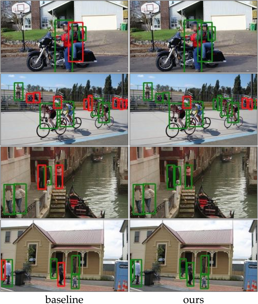
Figure 14: Qualitative improvements on the Pascal VOC person detection benchmark. Green and red bounding boxes denote correct and missing detections respectively.

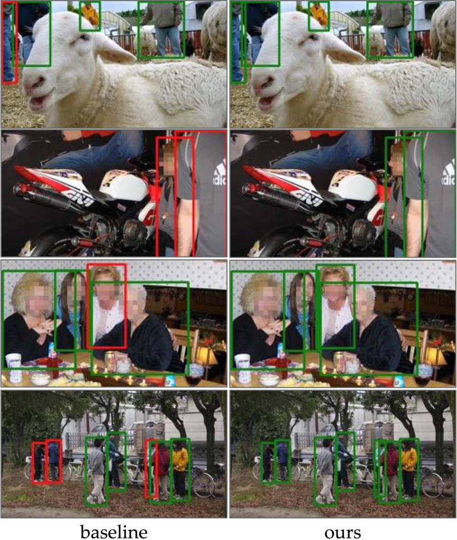
Figure 15: More qualitative improvements on the Pascal VOC person detection benchmark. Green and red bounding boxes denote correct and missing detections respectively.

References

- [1] Daniel J Butler, Jonas Wulff, Garrett B Stanley, and Michael J Black. A naturalistic open source movie for optical flow evaluation. In European Conference on Computer Vision, pages 611–625. Springer, 2012.
- [2] Ching-Hang Chen, Ambrish Tyagi, Amit Agrawal, Dylan Drover, Rohith MV, Stefan Stojanov, and James M. Rehg. Unsupervised 3d pose estimation with geometric self-supervision. In Proceedings of the IEEE Conference on Computer Vision and Pattern Recognition, 2019.
- [3] Ekin Dogus Cubuk, Barret Zoph, Dandelion Mané, Vijay Vasudevan, and Quoc V. Le. Autoaugment: Learning augmentation policies from data. CoRR, abs/1805.09501, 2018.
- [4] Santosh K. Divvala, Derek Hoiem, James H. Hays, Alexei A. Efros, and Martial Hebert. An empirical study of context in object detection. In Proc. IEEE Conf. on Computer Vision and Pattern Recognition (CVPR 09), pages 1271–1278, 2009.
- [5] Dylan Drover, Ching-Hang Chen, Amit Agrawal, Ambrish Tyagi, and Cong Phuoc Huynh. Can 3d pose be learned from 2d projections alone? In European Conference on Computer Vision Workshop, pages 78–94. Springer, 2018.
- [6] Nikita Dvornik, Julien Mairal, and Cordelia Schmid. Modeling visual context is key to augmenting object detection datasets. In IEEE European Conference on Computer Vision (ECCV), 2018.
- [7] Debidatta Dwibedi, Ishan Misra, and Martial Hebert. Cut, paste and learn: Surprisingly easy synthesis for instance detection. IEEE Conference on Computer Vision and Pattern Recognition (CVPR), 2017.
- [8] Mark Everingham, Luc Gool, Christopher K. Williams, John Winn, and Andrew Zisserman. The pascal visual object classes (voc) challenge. Int. J. Comput. Vision, 88(2):303–338, June 2010.
- [9] Alhussein Fawzi, Horst Samulowitz, Deepak Turaga, and Pascal Frossard. Adaptive data augmentation for image classification. In Proc. IEEE Intl. Conf. on Image Processing (ICIP 16), pages 3688–3692, 2016.
- [10] Georgios Georgakis, Arsalan Mousavian, Alexander C. Berg, and Jana Kosecka. Synthesizing training data for object detection in indoor scenes. CoRR, abs/1702.07836, 2017.
- [11] Georgios Georgakis, Md. Alimoor Reza, Arsalan Mousavian, Phi-Hung Le, and Jana Kosecka. Multiview RGB-D dataset for object instance detection. CoRR, abs/1609.07826, 2016.
- [12] Ross Girshick. Fast r-cnn. In Proceedings of the IEEE international conference on computer vision, pages 1440–1448, 2015.
- [13] Ishaan Gulrajani, Faruk Ahmed, Martín Arjovsky, Vincent Dumoulin, and Aaron C. Courville. Improved training of wasserstein gans. CoRR, abs/1704.00028, 2017.
- [14] Ankush Gupta, Andrea Vedaldi, and Andrew Zisserman. Synthetic Data for Text Localisation in Natural Images. In Proc. IEEE Conf. on Computer Vision and Pattern Recognition (CVPR 16), pages 2315–2324, 2016.
- [15] Søren Hauberg, Oren Freifeld, John W. Fisher III, and Lars Kai Hansen. Dreaming More Data: Class-dependent Distributions over Diffeomorphisms for Learned Data Augmentation. In Proceedings of the 19th International Conference on Artificial Intelligence and Statistics (AISTATS 16), volume JMLR: W&CP, pages 342–350, 2016.
- [16] Stefan Hinterstoisser, Vincent Lepetit, Paul Wohlhart, and Kurt Konolige. On pre-trained image features and synthetic images for deep learning. CoRR, abs/1710.10710, 2017.
- [17] Max Jaderberg, Karen Simonyan, Andrew Zisserman, and Koray Kavukcuoglu. Spatial transformer networks. CoRR, abs/1506.02025, 2015.
- [18] Long Jin, Justin Lazarow, and Zhuowen Tu. Introspective classification with convolutional nets. In I. Guyon, U. V. Luxburg, S. Bengio, H. Wallach, R. Fergus, S. Vishwanathan, and R. Garnett, editors, Advances in Neural Information Processing Systems 30, pages 823–833. Curran Associates, Inc., 2017.
- [19] S. Jin, A. RoyChowdhury, H. Jiang, A. Singh, A. Prasad, D. Chakraborty, and E. Learned-Miller. Unsupervised Hard Example Mining from Videos for Improved Object Detection. European Conference on Computer Vision (ECCV), 2018.
- [20] Anna Khoreva, Rodrigo Benenson, Eddy Ilg, Thomas Brox, and Bernt Schiele. Lucid data dreaming for multiple object tracking. arXiv preprint arXiv:1703.09554, 2017.
- [21] Diederik P. Kingma and Jimmy Ba. Adam: A method for stochastic optimization. CoRR, abs/1412.6980, 2014.
- [22] Philipp Krähenbühl. Free supervision from video games. In Proc. IEEE Conf. on Computer Vision and Pattern Recognition (CVPR 18), pages 2955–2964, 2018.
- [23] Kevin Lai, Liefeng Bo, Xiaofeng Ren, and Dieter Fox. A large-scale hierarchical multi-view rgb-d object dataset. 2011 IEEE International Conference on Robotics and Automation, pages 1817–1824, 2011.
- [24] Yann LeCun and Corinna Cortes. MNIST handwritten digit database. 2010.
- [25] Kwonjoon Lee, Weijian Xu, Fan Fan, and Zhuowen Tu. Wasserstein introspective neural networks. CoRR, abs/1711.08875, 2017.
- [26] Chen-Hsuan Lin, Ersin Yumer, Oliver Wang, Eli Schechtman, and Simon Lucey. ST-GAN: Spatial Transformer Generative Adversarial Networks for Image Compositing. In Proceedings of the IEEE Conference on Computer Vision and Pattern Recognition (CVPR 18), 2018.
- [27] Tsung-Yi Lin, Priya Goyal, Ross B. Girshick, Kaiming He, and Piotr Dollár. Focal loss for dense object detection. CoRR, abs/1708.02002, 2017.
- [28] Tsung-Yi Lin, Michael Maire, Serge J. Belongie, Lubomir D. Bourdev, Ross B. Girshick, James Hays, Pietro Perona, Deva Ramanan, Piotr Dollár, and C. Lawrence Zitnick. Microsoft COCO: common objects in context. CoRR, abs/1405.0312, 2014.
- [29] Wei Liu, Dragomir Anguelov, Dumitru Erhan, Christian Szegedy, Scott E. Reed, Cheng-Yang Fu, and Alexander C. Berg. SSD: single shot multibox detector. CoRR, abs/1512.02325, 2015.
- [30] Roozbeh Mottaghi, Xianjie Chen, Xiaobai Liu, Nam-Gyu Cho, Seong-Whan Lee, Sanja Fidler, Raquel Urtasun, and Alan Yuille. The Role of Context for Object Detection and Semantic Segmentation in the Wild. In Proceedings of the IEEE Conference on Computer Vision and Pattern Recognition (CVPR 14), pages 891–898, 2014.
- [31] Aude Oliva and Antonio Torralba. The role of context in object recognition. Trends in Cognitive Sciences, 11(12):520–527, 2007.
- [32] Alec Radford, Luke Metz, and Soumith Chintala. Unsupervised representation learning with deep convolutional generative adversarial networks. CoRR, abs/1511.06434, 2015.
- [33] Prajit Ramachandran, Barret Zoph, and Quoc V. Le. Searching for activation functions. CoRR, abs/1710.05941, 2017.
- [34] Alexander J Ratner, Henry R Ehrenberg, Zeshan Hussain, Jared Dunnmon, and Christopher Ré. Learning to Compose Domain-Specific Transformations for Data Augmentation. In Proceedings Advances in Neural Information Processing Systems 31 (NIPS 17), 2017.
- [35] Shaoqing Ren, Kaiming He, Ross B. Girshick, and Jian Sun. Faster R-CNN: towards real-time object detection with region proposal networks. CoRR, abs/1506.01497, 2015.
- [36] Stephan R Richter, Zeeshan Hayder, and Vladlen Koltun. Playing for benchmarks. In ICCV, 2017.
- [37] Tim Salimans, Ian Goodfellow, Vicki Cheung, Alec Radford, and Xi Chen. Improved Techniques for Training GANs. In Proceedings Advances in Neural Information Processing Systems 30 (NIPS 16), pages 1–10, 2016.
- [38] I. Sárándi, T. Linder, K. O. Arras, and B. Leibe. Synthetic Occlusion Augmentation with Volumetric Heatmaps for the 2018 ECCV PoseTrack Challenge on 3D Human Pose Estimation. ArXiv e-prints, Sept. 2018.
- [39] Abhinav Shrivastava, Abhinav Gupta, and Ross Girshick. Training region-based object detectors with online hard example mining. In Proceedings of the IEEE Conference on Computer Vision and Pattern Recognition, pages 761–769, 2016.
- [40] Abhinav Shrivastava, Abhinav Gupta, and Ross Girshick. Training region-based object detectors with online hard example mining. In Conference on Computer Vision and Pattern Recognition (CVPR), 2016.
- [41] Ashish Shrivastava, Tomas Pfister, Oncel Tuzel, Josh Susskind, Wenda Wang, and Russ Webb. Learning from simulated and unsupervised images through adversarial training. arXiv preprint arXiv:1612.07828, 2016.
- [42] K. Simonyan and A. Zisserman. Very deep convolutional networks for large-scale image recognition. CoRR, abs/1409.1556, 2014.
- [43] Arjun Singh, James Sha, Karthik S. Narayan, Tudor Achim, and Pieter Abbeel. Bigbird: A large-scale 3d database of object instances. 2014 IEEE International Conference on Robotics and Automation (ICRA), pages 509–516, 2014.
- [44] Yang Song, Rui Shu, Nate Kushman, and Stefano Ermon. Constructing unrestricted adversarial examples with generative models. In Advances in Neural Information Processing Systems, pages 8312–8323, 2018.
- [45] Fuwen Tan, Crispin Bernier, Benjamin Cohen, Vicente Ordonez, and Connelly Barnes. Where and who? automatic semantic-aware person composition. CoRR, abs/1706.01021, 2017.
- [46] Tijmen Tieleman. affnist dataset. 2013.
- [47] Toan Tran, Trung Pham, Gustavo Carneiro, Lyle Palmer, and Ian Reid. A Bayesian Data Augmentation Approach for Learning Deep Models. In Proceedings Advances in Neural Information Processing Systems 31 (NIPS 17), pages 1–10, 2017.
- [48] Jonathan Tremblay, Aayush Prakash, David Acuna, Mark Brophy, Varun Jampani, Cem Anil, Thang To, Eric Cameracci, Shaad Boochoon, and Stan Birchfield. Training deep networks with synthetic data: Bridging the reality gap by domain randomization. IEEE Conference on Computer Vision and Pattern Recognition (CVPR), 2018.
- [49] Gül Varol, Javier Romero, Xavier Martin, Naureen Mahmood, Michael J Black, Ivan Laptev, and Cordelia Schmid. Learning from synthetic humans.
- [50] Ting-Chun Wang, Ming-Yu Liu, Jun-Yan Zhu, Andrew Tao, Jan Kautz, and Bryan Catanzaro. High-resolution image synthesis and semantic manipulation with conditional gans. CoRR, abs/1711.11585, 2017.
- [51] Xiaolong Wang, Abhinav Shrivastava, and Abhinav Gupta. A-Fast-RCNN: Hard positive generation via adversary for object detection. In Proceedings of the IEEE Conference on Computer Vision and Pattern Recognition (CVPR 17), pages 2606–2615, 2017.
- [52] Yi Wu, Yuxin Wu, Georgia Gkioxari, and Yuandong Tian. Building generalizable agents with a realistic and rich 3d environment. arXiv preprint arXiv:1801.02209, 2018.
- [53] Chaowei Xiao, Jun-Yan Zhu, Bo Li, Warren He, Mingyan Liu, and Dawn Song. Spatially transformed adversarial examples. CoRR, abs/1801.02612, 2018.
- [54] Hao Yu, Zhaoning Zhang, Zheng Qin, Hao Wu, Dongsheng Li, Jun Zhao, and Xicheng Lu. Loss rank mining: A general hard example mining method for real-time detectors. CoRR, abs/1804.04606, 2018.
- [55] Yunhan Zhao, Ye Tian, Wei Shen, and Alan Yuille. Towards resisting large data variations via introspective learning. 2018.