Asymptotic dynamics of high dynamic range stratified turbulence

Abstract

Direct numerical simulations of homogeneous sheared and stably stratified turbulence are considered to probe the asymptotic high-dynamic range regime suggested by Gargett et al. (1984) and Shih et al. (2005). We consider statistically stationary configurations of the flow that span three decades in dynamic range defined by the separation between the Ozmidov length scale, $L_{O}=\sqrt{\epsilon/N^{3}}$, and the Kolmogorov length scale, $L_{K}=(\nu^{3}/\epsilon)^{1/4}$, up to $\mathrm{Re_{b}}\equiv(L_{O}/L_{K})^{4/3}=\epsilon/(\nu N^{2})\sim O(1000)$, where $\epsilon$ is the mean turbulent kinetic energy dissipation rate, $\nu$ is the kinematic viscosity, and $N$ is the buoyancy frequency. We isolate the effects of $\mathrm{Re_{b}}$, particularly on irreversible mixing, from the effects of other flow parameters of stratified and sheared turbulence (Mater and Venayagamoorthy, 2014). Specifically, we evaluate the influence of dynamic range independent of initial conditions. We present evidence that the flow approaches an asymptotic state for $\mathrm{Re_{b}}\gtrapprox 300$, characterized both by an asymptotic partitioning between the potential and kinetic energies and by the approach of components of the dissipation rate to their expected values under the assumption of isotropy. As $\mathrm{Re_{b}}$ increases above 100, there is a slight decrease in the turbulent flux coefficient $\Gamma=\chi/\epsilon$, where $\chi$ is the dissipation rate of buoyancy variance, but, for this flow, there is no evidence of the commonly suggested $\Gamma\propto\mathrm{Re_{b}}^{-1/2}$ dependence when $100\leq\mathrm{Re_{b}}\leq 1000$.

I Introduction

Sheared, stratified turbulence, energized by vertical shearing of horizontal motions in the presence of a statically stable density distribution, arises throughout the world’s oceans and atmosphere. Dynamical models of such flows, in particular capturing the vertical transport of heat due to irreversible mixing, are essential for modeling the global climate system because mixing occurs on relatively small scales, several orders of magnitude below those currently resolved in basin-scale models (Ivey et al., 2008; Ferrari and Wunsch, 2009; Gregg et al., 2018).

A key challenge for theoreticians is to develop a robust parameterization usable in such models for the vertical eddy diffusivity of heat $\kappa_{T}$ defined as

$$\kappa_{T}\equiv\frac{B}{N^{2}}\equiv\frac{\langle\frac{g}{\rho_{0}}w\rho\rangle}{N^{2}},\ N\equiv\sqrt{-\frac{g}{\rho_{0}}\frac{d\bar{\rho}}{dz}},$$ (1)

where angled brackets denote ensemble averaging, $B$ is the buoyancy flux, $N$ is the buoyancy frequency, $g$ is the constant gravitational acceleration, $\rho_{0}$ is a constant reference density, $(u,v,w)$ and $\rho$ are the fluctuating velocity vector and fluctuating density, respectively, in the $(x,y,z)$ coordinate system, and $\bar{\rho}$ is the mean ambient density with linear functional dependence in $z$. Here the Boussinesq approximation has been made such that density variations are sufficiently small so that a linear equation of state is appropriate and density variations are only significant in the buoyancy force.

Developing dynamical models of these complex flows has proved exceptionally difficult and controversial due not least to their potential dependence on a wide range of parameters (Mater and Venayagamoorthy, 2014; Ivey et al., 2018). For simplicity, we fix $\mathrm{Pr}=\nu/\kappa=1$, where $\nu$ is the kinematic viscosity and $\kappa$ is the molecular thermal diffusivity. Even with this assumption, stratified sheared turbulence is influenced by at least four independent length scales, associated with characteristic values of overall stratification, shear and both the intensity and decay rate of turbulence (Mater and Venayagamoorthy, 2014). The Ozmidov scale $L_{O}$, the Corrsin (or shear) scale $L_{C}$, the ‘large-eddy’ turbulent length scale $L_{L}$, and the Kolmogorov microscale $L_{K}$ are defined here as

$$\begin{aligned} L_{O}&\equiv\left({\frac{\epsilon}{N^{3}}}\right)^{1/2};\ &L_{C}&\equiv\left({\frac{\epsilon}{S^{3}}}\right)^{1/2};\\ L_{L}&\equiv\frac{E_{k}^{3/2}}{\epsilon};\ &L_{K}&\equiv\left(\frac{\nu^{3}}{\epsilon}\right)^{1/4},\end{aligned}$$ (2)

where $E_{k}$ is the averaged turbulent kinetic energy, $\epsilon$ is its dissipation rate and $S$ is the mean constant vertical shear, i.e. $S\equiv d\bar{u}/dz$ where $\bar{u}$ is the mean streamwise velocity with linear functional dependence in $z$. These four scales are determined by the properties of the fluctuation velocity field (i.e. the turbulence) relative to the background buoyancy frequency and shear. As noted by Ivey et al. (2018), it is entirely plausible that length scales comparing the perturbation scalar field to these background quantities may be more physically relevant, although particularly in such stationary flows such as those considered here, it is entirely plausible that the various length scales may become closely coupled (as we investigate further below).

Although in general the scales defined in (2) vary in space and time (see e.g. Mashayek et al., 2013), even in statistically stationary flows where characteristic values of these four length scales can be identified, parameterization of key properties of the flow could depend on at least three independent nondimensional parameters determined from these scales. Choices for these parameters are a characteristic Richardson number, $\mathrm{Ri}$, a turbulent Froude number $\mathrm{Fr}$ and the activity parameter $\mathrm{Re_{b}}$ (sometimes called the buoyancy Reynolds number and formally distinct from a related integral-scale quantity; see Portwood et al. (2016) for further discussion) defined as

$$\begin{gathered}\mathrm{Ri}\equiv\frac{N^{2}}{S^{2}}\equiv\left(\frac{L_{C}}{L_{O}}\right)^{4/3},\\ \mathrm{Fr}\equiv\frac{\epsilon}{NE_{k}}\equiv\left(\frac{L_{O}}{L_{L}}\right)^{2/3},\mathrm{Re_{b}}\equiv\frac{\epsilon}{\nu N^{2}}\equiv\left(\frac{L_{O}}{L_{K}}\right)^{4/3},\end{gathered}$$ (3)

although alternative parameters can be defined, such as a ‘shear number’ $\mathrm{S^{\ast}}\equiv(L_{L}/L_{C})^{2/3}\equiv SE_{k}/\epsilon\equiv 1/(\mathrm{Fr}\mathrm{Ri}^{1/2})$ and others (Mater and Venayagamoorthy, 2014).

In terms of these parameters, the central challenge regarding $\kappa_{T}$ becomes that of determining the functional dependence of $\kappa_{T}(\mathrm{Ri},\mathrm{Fr},\mathrm{Re_{b}})$. In a profoundly influential paper, Osborn (Osborn, 1980) argued from consideration of the turbulent kinetic energy equation that in stationary flows it is reasonable to suppose that the buoyancy flux $B$, or equivalently, for the stationary flows considered here, the dissipation rate of buoyancy variance $\chi$ defined as

$$\chi\equiv\kappa\left\langle\frac{g^{2}}{\rho_{0}^{2}N^{2}}{\left|\nabla\rho\right|^{2}}\right\rangle,$$ (4)

can be linearly related to the dissipation rate $\epsilon$ through a ‘turbulent flux coefficient’ or ‘mixing efficiency’ $\Gamma$, i.e. $\chi=\Gamma\epsilon$. Osborn hypothesized an upper bound for $\Gamma\leq 0.2$ on semi-empirical grounds, although in practice, $\Gamma$ is implemented as a constant saturating the upper bound(Gregg et al., 2018). The introduction of $\Gamma$ transforms the fundamental issue of modeling $\kappa_{T}$ into identifying the functional dependence of $\Gamma(\mathrm{Ri},\mathrm{Fr},\mathrm{Re_{b}})$, since $\kappa_{T}=\nu\Gamma\mathrm{Re_{b}}$ provided the flow is statistically stationary.

Many models have been presented for the functional dependence of $\Gamma$ based on observations, experiments and numerical simulations in a variety of different flows, with much recent activity (e.g. Ivey and Imberger, 1991; Barry et al., 2001; Shih et al., 2005; Ivey et al., 2008; Maffioli et al., 2016; Venaille et al., 2017; Salehipour et al., 2016a; Mashayek et al., 2017a; Zhou et al., 2017; Gregg et al., 2018; Monismith et al., 2018) though with little sign of consensus, due principally to three fundamental issues. Issue I is that disentangling transient and/or reversible processes from the irreversible processes crucial for quantifying and parameterizing mixing is extremely challenging. Issue II is that, even for flows where the assumption of stationarity is appropriate, stratification in a gravitational field and vertical shear both break isotropy, and so the extent to which anisotropy is important is difficult to determine, particularly when there is a relatively small dynamic range between $L_{K}$ and $\min(L_{C},L_{O})$ (as encountered by Gargett et al. (1984)). The condition $L_{C}<L_{O}$ is associated with growing and stationary flow configurations, as necessarily $\mathrm{Ri}<1$, suggesting that shear instabilities have to be sufficiently vigorous to sustain turbulence. This has the consequence that $L_{C}\gg L_{K}$ is a typical condition for high dynamic range, i.e. $\mathrm{Ri}\mathrm{Re_{b}}\gg 1$ by the relations defined in (3) and as suggested by Itsweire et al. (1993). Finally, issue III is that although in principle $\mathrm{Re_{b}}$, $\mathrm{Ri}$ and $\mathrm{Fr}$ are all independent parameters, there is emerging evidence (e.g. Lucas and Caulfield, 2017) that in many flows the parameters become correlated, and so an apparent dependency of $\kappa_{T}$ or $\Gamma$ on one parameter is actually associated with variation in another parameter.

To address all three issues, we consider the model flow of stationary homogeneous sheared and stratified turbulence (S-HSST)(e.g. Holt et al., 1992; Itsweire et al., 1993; Jacobitz et al., 1997; Shih et al., 2005). In S-HSST, the production of turbulent kinetic energy by uniform mean vertical shear exactly balances the dissipation rates of kinetic and potential energy by molecular motion, addressing issue I by ensuring energetic stationarity by design. When numerically simulated, the turbulence fills the flow domain provided that $\mathrm{Re_{b}}$ is sufficiently large (Stillinger et al., 1983). More generally, stratified turbulence has been shown to exhibit different dynamics depending on the value of $\mathrm{Re_{b}}$ (Shih et al., 2005; Hebert and de Bruyn Kops, 2006; Bartello and Tobias, 2013; de Bruyn Kops, 2015; de Bruyn Kops and Riley, 2019). Gargett et al. (1984) observed in limited two-point statistics from ocean data that Kolmogorov-Oboukhov-Corrsin (KOC) scaling may be observed in stratified turbulence when $\mathrm{Re_{b}}\sim O(10^{3})$ and higher. de Bruyn Kops (2015) observes that KOC scaling is generally not observed in DNS up to $\mathrm{Re_{b}}=220$, though some statistics may be consistent with such scalings. An important open question is thus how stratified turbulence behaves when $\mathrm{Re_{b}}>O(100)$, a parameter space accessible by modern simulations of S-HSST with sufficiently small $\mathrm{Fr}$ for the stratification to have a first-order effect on the turbulent dynamics. However, to address issue II there is the further constraint that $\mathrm{Ri}\mathrm{Re_{b}}\gg 1$.

In fact, in S-HSST $\mathrm{Ri}$ and $\mathrm{Fr}$ cease to be free, but rather must adjust to ensure statistical stationarity. It has been empirically observed in simulations that the various dynamic length scales ‘tune’ so that $\mathrm{Fr}\approx 0.5$ and $\mathrm{Ri}\approx 0.16$, and equivalently $\mathrm{S^{\ast}}\approx 5$. An immediate consequence of the emergence of an apparently $\mathrm{Re_{b}}-$invariant stationary value of $\mathrm{Ri}$ in S-HSST is that issue II can indeed be addressed at sufficiently large $\mathrm{Re_{b}}$.

Perhaps more importantly, issue III is also addressed, as the dependence of flow properties on $\mathrm{Re_{b}}$ can be probed independently of the other parameters. Specifically, although the adjustment of $\mathrm{Fr}\approx 0.5$ and $\mathrm{Ri}\approx 0.16$ occurs at $\mathrm{Re_{b}}\sim O(10)$, other dynamical scalings have been observed to change as $\mathrm{Re_{b}}$ increases beyond $\mathrm{Re_{b}}\sim O(100)$ (Shih et al., 2005; de Bruyn Kops, 2015). The objective of this study is thus to investigate how the key properties of the turbulence, in particular the energy partitioning, mixing and small-scale anisotropy depend on variations of $\mathrm{Re_{b}}$. A specific question to investigate is whether the postulated power law $\Gamma\propto\mathrm{Re_{b}}^{-1/2}$ (Shih et al., 2005; Ivey et al., 2008; Monismith et al., 2018) for sufficiently large $\mathrm{Re_{b}}$ occurs in this flow in which dependence on other flow parameters can be completely eliminated.

II Simulations

The incompressible Navier-Stokes equations are considered, subject to the nonhydrostatic Boussinesq approximation and coupled with equations for continuity and buoyancy transport. A turbulent decomposition is performed relative to a mean buoyancy gradient and a mean streamwise velocity gradient, both in the vertical direction (see also Rogallo, 1981; Holt et al., 1992; Jacobitz et al., 1997; Shih et al., 2000). We implement the system with the same Fourier pseudo-spectral scheme described by (Almalkie and de Bruyn Kops, 2012; de Bruyn Kops, 2015), except that an additional shear term is handled by an integration factor (Brucker et al., 2007; Chung and Matheou, 2012; Sekimoto et al., 2016).

Stationarity is induced by fixing a value of $\nu$, choosing a target turbulent kinetic energy $E_{t}$ then adjusting the Richardson number via $g$ (c.f. Taylor et al., 2016) using a mass-spring-damper control system:

$$c_{0}S\mathrm{Ri}^{\prime}(t)+2\alpha\omega\tilde{E}_{k}^{\prime}(t)+\omega^{2}(\tilde{E}_{k}(t)-1)=0$$ (5)

where the prime notation denotes a temporal derivative, $\tilde{E}_{k}(t)\equiv E_{k}/E_{t}$ is the normalized turbulent kinetic energy, $\omega$ is the characteristic frequency of oscillation and $\alpha$ is a dimensionless damping factor. The control system has been derived by assuming that the kinetic energy follows a second order linear system (e.g. Rao and de Bruyn Kops, 2011), and then by applying the first-order approximation $\tilde{E}_{k}^{\prime}(t)\approx c_{0}S(\mathrm{Ri}(t)-\mathrm{Ri}_{c})$ such that $\tilde{E}_{k}^{\prime\prime}(t)\approx c_{0}S\mathrm{Ri}^{\prime}(t)$. The parameter $c_{0}\approx-1$ is supported by Jacobitz et al. (1997), the characteristic frequency $\omega$ is determined by the mean shear, and a damping coefficient $\alpha=1.5$ was found to work well.

Crucially, following this procedure, $\mathrm{Ri}\approx 0.16$ emerges without presupposition for all our cases, as shown in the table 1 along with other emergent parameters; flow statistics are averaged over a period of $St\approx 100$ unless noted otherwise.

Case	$\mathrm{Re_{b}}$	$\mathrm{Ri}$	$\mathrm{Fr}$	$N_{x}$
SHSST-R1	36	0.163	0.46	1024
R2	48	0.159	0.47	1280
R3	59	0.162	0.48	1536
R4	81	0.154	0.50	1792
R5	110	0.155	0.52	2048
R6	160	0.157	0.48	3072
R7	240	0.156	0.48	4096
R8	390	0.146	0.46	6144
R9	550	0.163	0.45	8192
R10	900	0.152	0.42	9600

Table 1: Simulation parameters. $N_{x}$ is the number of grid points in the $x$-direction and the grid spacing is isotropic.

Furthermore, the dissipation rate $\epsilon$ also ‘tunes’ such that $\mathrm{Fr}\approx 0.5$. As the dissipation rate is an emergent quantity, the smallest length scales are resolved by adjusting the resolution such that $k_{max}L_{K}\approx 2$, where $k_{max}$ is the largest Fourier domain wavenumber. We also found it necessary to use a relatively large domain with $L_{x}/L_{y}=2$, $L_{x}/L_{z}=4$ and $L_{x}/L_{L}\approx 40$, where $L_{x}$, $L_{y}$, and $L_{z}$ are the dimensions of the domain, in order to support the anisotropic large scales of the flow.

III Results and discussion

III.1 Energetics

We stress that, although $E_{k}\approx E_{t}$ is enforced, the parameters $\mathrm{Ri}$, $\mathrm{Fr}$ and $\mathrm{Re_{b}}$ emerge from the simulations, as do the structure of the turbulence and the scalar. We consider the ratio of the potential energy to kinetic energy, $\mathrm{R_{PK}}\equiv E_{p}/E_{k}$, and the ratio of the potential energy to the kinetic energy of vertical motion, $\mathrm{R_{PV}}\equiv E_{p}/E_{v}$ where the energies are defined as:

$$E_{v}\equiv\frac{1}{2}\langle{w^{2}}\rangle\;\text{and}\;E_{p}\equiv\frac{1}{2}\left<\frac{g^{2}/\rho_{0}^{2}}{N^{2}}{\rho^{2}}\right>\text{ .}$$

Energy-partitioning is a critical component to mixing models wherein Reynolds number, or $\mathrm{Re_{b}}$, dependence is often omitted and the mixing is assumed to be a function of $\mathrm{Ri}$ (Osborn and Cox, 1972; Schumann and Gerz, 1995; Pouquet et al., 2018). Furthermore, in ‘strongly’ stratified turbulent flow, Billant and Chomaz (2001) suggest that there should be approximate equipartition between potential and kinetic energy, i.e. $\mathrm{R_{PK}}\approx 1$, an assumption also used by Lindborg (2006). Figure 1 illustrates that this basic assumption of equipartition is not appropriate. Perhaps more interesting, the energy ratios decrease by a factor of two relative to the lowest $\mathrm{Re_{b}}$ case until $\mathrm{Re_{b}}\approx 300$, after which the energy ratios appear to remain constant with anisotropy of velocity variance explaining the different behaviors of $\mathrm{R_{PK}}$ and $\mathrm{R_{PV}}$.

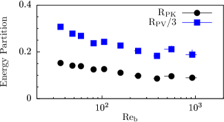
Figure 1: Energy partitions as a function of $\mathrm{Re_{b}}$. Bars indicate upper and lower quartile measurements of instantaneous quantities.

III.2 Small-scale anisotropy

The observation of anisotropy in the energy partitions of the previous section is particularly important, due not least to the inevitable requirement to estimate energetic dissipation rates in circumstances where each component of the rate-of-deformation tensor is not available. The existence of anisotropy at dissipative length scales would require dynamical estimates of $\kappa_{T}$ to account for anisotropy. Therefore, it is necessary to evaluate common dissipation surrogate models to assess their applicability and to characterize small-scale anisotropy in these flows. Here, we use single component surrogate models which rely on a single derivative and the isotropy assumption:

$$\tilde{\epsilon}_{ij} =\begin{cases}15\nu\left\langle\big{(}\frac{\partial u_{i}}{\partial x_{j}}\big{)}^{2}\right\rangle&\text{if $i=j$}\\ 15/2\nu\left\langle\big{(}\frac{\partial u_{i}}{\partial x_{j}}\big{)}^{2}\right\rangle&\text{if $i\neq j$}\end{cases}$$ (6a)

$$\tilde{\chi}_{j} =3\kappa\left\langle\frac{g^{2}}{\rho_{0}^{2}N^{2}}\left(\frac{\partial\rho}{\partial x_{j}}\right)^{2}\right\rangle\text{ .}$$ (6b)

In flows that are inherently anisotropic due to mean shear or mean flux, it is widely assumed that small-scale isotropy is a reasonable assumption when the scale separation is large (e.g. Gargett et al., 1984). However, evidence suggests that isotropy assumptions can be very inaccurate in stably stratified flows at finite $\mathrm{Re_{b}}$ (Itsweire et al., 1993; Hebert and de Bruyn Kops, 2006; de Bruyn Kops, 2015; de Bruyn Kops and Riley, 2019).

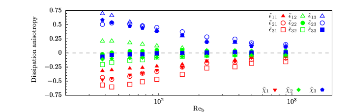
Figure 2: Instantaneous measurements of small-scale anisotropy. The dashed line represents perfect isotropy at small scales.

The validity of (6) is tested with the help of figure 2 in which is plotted the relative error $(\tilde{\epsilon}_{ij}-\epsilon)/\epsilon$ of the various single-component dissipation estimates. As with energy partition, there is an apparently asymptotic regime for $\mathrm{Re_{b}}\gtrapprox 300$ in which the assumption of isotropy applied to dissipation rate becomes valid within approximately 15% error. Nevertheless, there is evidence of small-scale anisotropy as expected from the analysis in Durbin and Speziale (1991), which shows that dissipation-range isotropy should only exist when $\mathrm{S^{\ast}}\ll 1$; in these simulated flows $\mathrm{S^{\ast}}\approx 5$. However, we observe that $\tilde{\epsilon}_{22}$, $\tilde{\epsilon}_{33}$, and $\tilde{\chi}_{2}$ yield good estimates of the dissipation rates even in cases in which the small scales are strongly anisotropic.

III.3 Mixing coefficient

We plot the turbulent mixing coefficient $\Gamma\equiv\chi/\epsilon$ in figure 3a. Whereas there is some modest decrease with increasing $\mathrm{Re_{b}}$ from the peak $\Gamma$ of approximately 0.19, remarkably close to Osborn’s suggested upper bound, there is no evidence of the commonly-suggested $\mathrm{Re_{b}}^{-1/2}$ scaling (e.g. Shih et al., 2005; Ivey et al., 2008; Monismith et al., 2018). A decrease in mixing efficiency with respect to $\mathrm{Re_{b}}$ is observed until $\mathrm{Re_{b}}\approx 200$, above which $\Gamma\approx 0.17$. There is no evidence of the ‘energetic’ regime of Shih et al. (2005) for $\mathrm{Re_{b}}>100$, suggesting that transient multi-parameter effects may well be relevant in the evolution of their flows such that $\mathrm{Re_{b}}$ is not always an independent parameter (see issue III as described in §1). There is evidence that the upper bound proposed by Osborn is a useful estimate, at least in flows where the underlying assumption of stationarity is well-justified, as such flows naturally adjust to $\mathrm{Ri}\approx 0.16$ and $\mathrm{Fr}\approx 0.5$.

Alternative descriptions of the mixing behavior are instructive. In the asymptotically high $\mathrm{Re_{b}}$ regime, the buoyancy variance dissipation rate adjusts such that $\chi\approx E_{p}N$ as evidenced by figures 1 and 3. Although this is a natural scaling, it is of interest that the $O(1)$ constant is actually extremely close to $1$. A second instructive description of mixing is the turbulent Prandtl number $\mathrm{Pr_{T}}=\kappa_{M}/\kappa_{T}$, where $\kappa_{M}$ is the eddy diffusivity of momentum:

$$\kappa_{M}\equiv\frac{\langle uw\rangle}{S}=\frac{P}{S^{2}},$$ (7)

and $P$ is the production rate of turbulent kinetic energy. Therefore,

$$\mathrm{Pr_{T}}=\frac{N^{2}}{S^{2}}\frac{P}{B}\equiv\frac{\mathrm{Ri}}{\mathrm{Rf}}\approx\frac{\mathrm{Ri}(1+\Gamma)}{\Gamma},$$ (8)

where $\mathrm{Rf}$ is the ‘flux Richardson number’, and the relationships $P\approx B+\epsilon=\chi+\epsilon$ in a stationary flow has been used. $\mathrm{Pr_{T}}$ is plotted in 3b, and proves to be close to one for all values of $\mathrm{Re_{b}}$. This is perhaps unsurprising, but makes clear that the turbulent processes that mix heat and momentum in these flows are highly coupled, and in particular that the stratification is not sufficiently ‘strong’ to modify the turbulent processes greatly, but rather that the irreversible conversion of kinetic into potential energy occurs in a balanced, equilibrated way.

Using mixing length arguments, Odier et al. (2009) defined:

$$L_{\rho}\equiv\left(\frac{B}{N^{2}S}\right)^{1/2};\ L_{m}\equiv\left(\frac{P}{S^{3}}\right)^{1/2};$$ (9)

such that $L^{2}_{m}/L^{2}_{\rho}=Pr_{T}$. Therefore, since for our flows $Pr_{T}\approx 1$ and $P\approx(1+\Gamma)\epsilon$, it is apparent that the density length scale at the heart of the model presented by Ivey et al. (2018) is coupled to the Corrsin scale by $L_{\rho}/L_{C}=\sqrt{1+\Gamma}$, and the key parameter $D\equiv\chi/\epsilon=1/\Gamma$ has nearly fixed value.

IV Conclusions

We have used a canonical controlled flow to evaluate the isolated effects of high dynamic range in sheared stratified turbulent flow. The energy partitioning varies non-trivially where $\mathrm{Re_{b}}\lessapprox 300$ above which an apparently asymptotic regime is entered, consistent with (Gargett et al., 1984; de Bruyn Kops, 2015). The flow retains measurable anisotropy at dissipation scales, as suggested by the analyses of Durbin and Speziale (1991), at all values of $\mathrm{Re_{b}}$ we have considered. Nevertheless, some single-component surrogates exist which accurately estimate dissipation rates via isotropy assumptions even for smaller $\mathrm{Re_{b}}$.

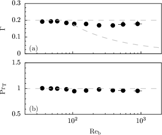
Figure 3: a: Variation of turbulent flux coefficient $\Gamma$ with $\mathrm{Re_{b}}$. The upper bound proposed by Osborn is indicated by the gray dashed line where $\Gamma\approx 0.2$, and the $\mathrm{Re_{b}}^{-1/2}$-based parameterization suggested in Shih et al. (2005) is plotted for their ‘energetic’ regime of $\mathrm{Re_{b}}>100$. b: Variation of turbulent Prandtl number $\mathrm{Pr_{T}}$ with $\mathrm{Re_{b}}$.

The results presented here seem to indicate that the effects of the large dynamic-range regimes explored by Gargett et al. are strongly influenced by asymptotic scalar density dynamics, rather than by the velocity field independently. Nevertheless, the measured mixing is a much weaker function of $\mathrm{Re_{b}}$ compared to some proposed scalings (Shih et al., 2005), with the turbulent Prandtl number $\mathrm{Pr_{T}}\approx 1$ and the turbulent mixing coefficient $\Gamma$ near the classical bound of $0.2$ as suggested by Osborn, although decreasing slightly for $\mathrm{Re_{b}}\lessapprox 300$. The application of these results to higher Prandtl numbers merits further study, where dynamic range arguments indicate transition at lower $\mathrm{Re_{b}}$ as $\mathrm{Pr}$ is increased.

We stress that the flow we have considered has, by design, controlled dependence on all other parameters. $\mathrm{Ri}\approx 0.16$ and $\mathrm{Fr}\approx 0.5$ naturally emerge to ensure stationarity. Therefore, we conjecture that observed apparent variation of mixing properties with $\mathrm{Re_{b}}$ (Monismith et al., 2018) can be explained by breaking one or the other of these constraints, i.e. the variation is due to either transient effects, well-known to lead to strong variation in mixing properties (e.g Salehipour et al., 2016b; Mashayek et al., 2017b), or ‘hidden’ and perhaps correlated variation with other parameters (e.g Zhou et al., 2017). Additionally, there could also be as yet unquantified strong dependence on initial or boundary conditions, whereas the flow we have considered is isolated from such effects. To develop robust mixing parameterizations, it is necessary to develop appropriate models to capture the effects of such conditions, informed by and generalizing from such controlled, idealized flows as considered here.