Nonlocal minimal graphs in the plane
are generically sticky

Abstract.

We prove that nonlocal minimal graphs in the plane exhibit generically stickiness effects and boundary discontinuities. More precisely, we show that if a nonlocal minimal graph in a slab is continuous up to the boundary, then arbitrarily small perturbations of the far-away data produce boundary discontinuities.

Hence, either a nonlocal minimal graph is discontinuous at the boundary, or a small perturbation of the prescribed conditions produces boundary discontinuities.

The proof relies on a sliding method combined with a fine boundary regularity analysis, based on a discontinuity/smoothness alternative. Namely, we establish that nonlocal minimal graphs are either discontinuous at the boundary or their derivative is Hölder continuous up to the boundary. In this spirit, we prove that the boundary regularity of nonlocal minimal graphs in the plane “jumps” from discontinuous to $C^{1,\gamma}$, with no intermediate possibilities allowed.

In particular, we deduce that the nonlocal curvature equation is always satisfied up to the boundary.

As an interesting byproduct of our analysis, one obtains a detailed understanding of the “switch” between the regime of continuous (and hence differentiable) nonlocal minimal graphs to that of discontinuous (and hence with differentiable inverse) ones.

E-mail addresses: serena.dipierro@uwa.edu.au, savin@math.columbia.edu, enrico.valdinoci@uwa.edu.au

1. Introduction

Nonlocal minimal surfaces have been introduced in [MR2675483] with the aim of comprising long range effects in a variational problem resembling the one arising from the minimization of the classical perimeter functional and of modeling concrete problems in which remote interactions play a decisive role.

Specifically, given $s\in(0,1)$, one considers the long range interaction of two disjoint (measurable) sets $F$, $G\subseteq\mathbb{R}^{n}$ given by

$${\mathcal{I}}_{s}(F,G):=\iint_{F\times G}\frac{dx\,dy}{|x-y|^{n+s}}.$$ (1.1)

For a bounded reference domain $\Omega$ with Lipschitz boundary, one also defines the $s$-perimeter of a set $E\subseteq\mathbb{R}^{n}$ in $\Omega$ as

$${\rm Per}_{s}(E;\Omega):={\mathcal{I}}_{s}(E\cap\Omega,E^{c}\cap\Omega)+{\mathcal{I}}_{s}(E\cap\Omega,E^{c}\cap\Omega^{c})+{\mathcal{I}}_{s}(E\cap\Omega^{c},E^{c}\cap\Omega),$$

where the superscript “$c$” denotes the complementary set in $\mathbb{R}^{n}$.

One says that $E$ is $s$-minimal in $\Omega$ if ${\rm Per}_{s}(E;\Omega)<+\infty$ and

$${\rm Per}_{s}(E;\Omega)\leqslant{\rm Per}_{s}(E^{\prime};\Omega)$$ (1.2)

for every $E^{\prime}\subseteq\mathbb{R}^{n}$ such that $E^{\prime}\cap\Omega^{c}=E\cap\Omega^{c}$.

An intense research activity was recently focused on $s$-minimal sets. Among the many topics covered, such a research took into account:

• Asymptotics: as $s\nearrow 1$, the $s$-perimeter recovers the classical perimeter, see [MR1945278, MR1942130, MR2782803, MR2765717, MR3161386], and as $s\searrow 0$ the problem is related to Lebesgue measure, see [MR1940355, MR3007726].

• Interior regularity: $s$-minimal sets have $C^{\infty}$ boundary when $n=2$, and also when $n\leqslant 7$ provided that $s\in(1-\varepsilon_{0},1)$ for a sufficiently small $\varepsilon_{0}\in(0,1)$, see [MR3090533, MR3107529, MR3331523]. One can also consider regularity problems for stable, rather than minimal, objects, see [BV, CCC].

• Bernstein property: $s$-minimal sets with a graphical structure are necessarily half-spaces in dimension $n\leqslant 3$, and also in dimension $n\leqslant 8$ provided that $s\in(1-\varepsilon_{0},1)$ for a sufficiently small $\varepsilon_{0}\in(0,1)$, see [MR3680376, FAR]. More generally, one can prove similar results assuming only that some partial derivatives of the graph are bounded from either above or below, see [FMOS].

• Isoperimetric problems: minimizing the $s$-perimeter under suitable volume conditions naturally leads to a number of fractional isoperimetric problems, see [MR2469027, MR2799577, MR3322379, MR3412379].

• Growth at infinity: if an $s$-minimal set is the graph of a function $u$, then the gradient of $u$ is bounded in the interior of a ball by a power of its oscillation, see [COZCAB]. From this and [MR3331523], one obtains also the $C^{\infty}$-regularity of $u$.

• Connection to the fractional Allen-Cahn equation: minimizers of long range phase transition models and of fractional Allen-Cahn energy functionals approach, at a large scale, nonlocal minimal surfaces [MR2948285, MR3133422, MR3900821]. This fact makes geometric techniques available in the study of the symmetry properties of the solutions of the fractional Allen-Cahn equation and for nonlinear boundary reaction equations, in the spirit of a classical conjecture by Ennio De Giorgi, see [MR2177165, MR2498561, MR2644786, MR3148114, MR3280032, MR3610941, DEGIO, MR3812860, SAV2, FSERRA, GUI].

• Connection with spin models in statistical mechanics: ground states for long-range Ising models and nonlocal minimal surfaces approximate each other in a suitable $\Gamma$-convergence setting, see [MR3652519].

• Free boundary problems: Several new free boundary problems have been studied by taking into account the nonlocal perimeter as interfacial energy, see [MR3390089, MR3427047, MR3678490, MR3712006].

• Surfaces of constant nonlocal mean curvature: minimizers of the fractional perimeter satisfy a suitable Euler-Lagrange equation, which can be written in the form

  $$\int_{\mathbb{R}^{n}}\frac{\chi_{E^{c}}(y)-\chi_{E}(y)}{|x-y|^{n+s}}\,dy=0,\qquad x\in(\partial E)\cap\Omega.$$

  In analogy with the classical case, the left hand side of this equation can be considered as a nonlocal mean curvature (or simply a nonlocal curvature when $n=2$). It is natural to consider curves, surfaces and hypersurfaces with vanishing, or prescribed, nonlocal mean curvature, see e.g. [MR3485130, MR3770173, MR3744919, MR3836150, MR3881478] for a number of results in this direction.

• Geometric flows: In analogy with the classical case, one can also consider geometric evolution equations of nonlocal type, such as the evolution of a hypersurface with normal velocity equal to the nonlocal mean curvature, see e.g. [MR2487027, MR2564467, MR3401008, MR3713894, MR3778164, SAEZ]. This type of geometric motions also appears as a limit of discrete heat flows and can be seen as a toy model for the evolution of cellular automata, with potential applications in population dynamics.

• Nonlocal capillarity problems: Nonlocal interactions as the ones in (1.1) have been also exploited to model capillarity phenomena in which the shape of the droplets are influenced by long range interactions, see [MR3717439, MR3707346]: in particular, in this context, one can describe the contact angle between the droplet and the container in terms of a suitable nonlocal Young’s Law.

Furthermore, nonlocal perimeters and related fractional operators have been studied also from the numerical point of view, also due to their flexibility in image reconstruction theory, see e.g. [MR3413590, MR3893441, NOCHETTO].

Hence, in general, the nonlocal perimeter functional provides a burgeoning topic of research which is experiencing an intense activity in many directions, involving mathematicians with different backgrounds and combining different methodologies coming from geometric analysis, partial differential equations, geometric measure theory, calculus of variations and functional analysis.

Since now, all the problems covered in this framework, the methods exploited and the results obtained have shown significant differences with respect to their classical analogues, and the new features provided by the nonlocal aspect of the problem turned out to play a very major role.

We also refer to [MR3588123, MR3824212] for recent surveys on nonlocal minimal surfaces and related topics.

Going back to the minimization problem in (1.2), for unbounded domains $\Omega$, the $s$-perimeter of many “interesting sets” can become unbounded. Nevertheless, one can make sense of the minimization procedure by saying that $E$ is locally $s$-minimal in a (possibly unbounded) domain $\Omega$ if $E$ is $s$-minimal in every bounded and Lipschitz domain $\Omega^{\prime}\Subset\Omega$ (see Section 1.3 in [MR3827804] for additional details on these minimality notions).

In particular, in this way, one can take into account the local minimization problem on cylindrical domains of the form $B\times\mathbb{R}$, where $B\subset\mathbb{R}^{n-1}$ is a bounded set with smooth boundary. This setting naturally comprises the one of “graphs”, i.e. sets which happen to be the subgraph of a certain function. The graphical setting was studied in detail in [MR3516886], establishing that a locally $s$-minimal set which is graphical outside a cylinder is necessarily graphical over the entire space.

In this setting, the locally $s$-minimal set is described by a uniformly continuous graph inside the cylinder which can exhibit boundary discontinuities of jump type, that is the boundary datum is not necessarily attained continuously – even for smooth and compactly supported data, as shown by an example in [MR3596708].

In jargon, $s$-minimal sets with graphical properties are called $s$-minimal graphs, and the boundary discontinuity phenomenon is known with the name of “stickiness” (meaning that the interior $s$-minimal surface has to stick at the walls of the cylinder to attain its exterior datum).

Of course, this stickiness phenomenon is a purely nonlocal feature, since classical minimal surfaces leave convex domain in a transversal fashion, and it seems to be a very distinctive phenomenon for nonlocal minimal surfaces that is not shared by other problems of fractional type (e.g., solutions of fractional Laplace equations do not exhibit jumps at the boundary).

The main goal of this article is to show that this stickiness phenomenon and the corresponding boundary discontinuity for nonlocal minimal graphs in the plane, as introduced in [MR3516886, MR3596708], is indeed a “generic” feature. More precisely, we show that either a nonlocal minimal graph in the plane is boundary discontinuous, or there is an arbitrarily small perturbation of its exterior data which produces a boundary discontinuous nonlocal minimal graph. In this sense, boundary continuity is an “unstable” property of nonlocal minimal graphs, since it is destroyed by arbitrarily small perturbations, and the stickiness phenomenon holds true “essentially” for all prescribed exterior data. Our precise result is the following:

Theorem 1.1 (Genericity of the stickiness phenomenon).

Let ${{\alpha}}\in(s,1)$ and $\Omega:=(0,1)\times\mathbb{R}$. Let $v\in C^{1,{{\alpha}}}(\mathbb{R})$. Let $\varphi\in C^{1,{{\alpha}}}(\mathbb{R},[0,+\infty))$ be not identically zero, with $\varphi=0$ in $(-d,1+d)$, for some $d>0$.

Let $u:\mathbb{R}\times[0,+\infty)\to\mathbb{R}$ be defined, for all $t\geqslant 0$, by

$$u(x_{1},t):=v(x_{1})+t\varphi(x_{1})\qquad{\mbox{ if~{}$x_{1}\in\mathbb{R}\setminus(0,1)$,}}$$

and, for $x_{1}\in(0,1)$, by requiring that the subgraph

$$E_{t}:=\{x=(x_{1},x_{2})\in\mathbb{R}^{2}{\mbox{ s.t. }}x_{2}<u(x_{1},t)\}$$ (1.3)

is locally $s$-minimal in $\Omega$.

Assume that

$$\lim_{{x_{1}\searrow 0}}u(x_{1},0)=v(0).$$ (1.4)

Then, for any $t>0$,

$$\limsup_{{x_{1}\searrow 0}}u(x_{1},t)>v(0).$$ (1.5)

Concerning the definition of $u(x_{1},t)$ in Theorem 1.1, we recall that any $s$-minimal set given by exterior data with a graphical structure has also a graphical structure, thanks to [MR3516886], therefore the set $E_{t}$ in (1.3) is indeed a subgraph.

The proof of Theorem 1.1 relies on an auxiliary boundary regularity result, that we now state. This result seems to be very interesting in itself, since it rules out “intermediate” pathologies in the regularity theory. Namely:

• On the one hand, nonlocal minimal graphs can well be discontinuous at the boundary (as the example in [MR3596708]).

• On the other hand, we prove that if nonlocal minimal graphs happen to be continuous at the boundary, then they are necessarily differentiable, and the derivative is Hölder continuous.

In addition, the Hölder exponent can be explicitly determined, and it will be sufficiently large for concrete applications.

In particular, we establish that no halfway boundary regularity is possible for nonlocal minimal graphs: they cannot be merely continuous, or Hölder, or Lipschitz, since the absence of boundary jumps is sufficient to differentiability and Hölder regularity of the derivative.

The precise statement that we prove is the following:

Theorem 1.2 (Continuity implies differentiability).

Let ${{\alpha}}\in(s,1)$, $u:\mathbb{R}\to\mathbb{R}$, with $u\in C^{1,{{\alpha}}}([-h,0])$ for some $h\in(0,1)$, and

$$E:=\{(x_{1},x_{2})\in\mathbb{R}^{2}{\mbox{ s.t. }}x_{2}<u(x_{1})\}.$$

Assume that $E$ is locally $s$-minimal in $(0,1)\times\mathbb{R}$. Suppose also that

$$\lim_{x_{1}\searrow 0}u(x_{1})=\lim_{x_{1}\nearrow 0}u(x_{1}).$$ (1.6)

Then, $u\in C^{1,\gamma}([-h,1/2])$, with

$$\gamma:=\min\left\{{{\alpha}},\,\frac{1+s}{2}\right\}.$$

We think that Theorem 1.2 possesses some surprising features. First of all, at a first glance, the boundary regularity of Theorem 1.2 seems “too good to be true” when compared with the case of nonlocal linear equations, in which solutions are in general not better than Hölder continuous at the boundary. In this sense, the regularity obtained in Theorem 1.2 arises from the combination of two distinctive properties, namely an improvement of flatness method, which is specific for nonlocal minimal surfaces, and that we perform here at boundary points, and the higher order boundary regularity for linear equations. The first of these two ingredients provides a differentiability result, and only after this the second ingredient comes into play. Namely, we will exploit the linear theory only after having determined that the linear equation is a “very good approximation” of the nonlocal curvature equation “with respect to its own tangent direction”. In this way, having already established a differentiability result by the improvement of flatness method, the linear theory necessarily forces the first term in the boundary expansion to vanish, and hence the second term of the expansion becomes representative of the boundary regularity (this justifies the exponent $1+\frac{1+s}{2}$ in Theorem 1.2, since the linearized equation in this case is related to the fractional Laplacian of order $\frac{1+s}{2}$, and the exponent $1+\frac{1+s}{2}$ is precisely the one arising from the second term in the boundary expansion).

Another very intriguing feature given by Theorem 1.2 is that the switch between “non-sticky” and “sticky” nonlocal minimal graphs is continuous in $L^{\infty}$ but not in $C^{1}$. That is, if one considers a nonlocal minimal graph which is continuous up to the boundary, then it is in fact $C^{1,\frac{1+s}{2}}$-regular by Theorem 1.2, and, according to Theorem 1.1, a small perturbation of the exterior data makes this $C^{1,\frac{1+s}{2}}$-graph switch to a discontinuous graph. If the perturbation is small, the two graphs are close to each other, nevertheless their boundary derivative is very different, since in the unperturbed case the graph detaches in a $C^{1,\frac{1+s}{2}}$-way from any prescribed tangent direction, while in the perturbed case the graph detaches in a $C^{1,\frac{1+s}{2}}$-way from the vertical direction (in particular, any small perturbation of the exterior data makes the boundary derivative pass suddenly from a given, possibly zero, value to infinity).

      

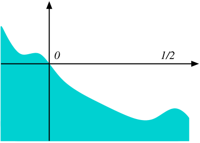
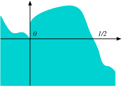
Figure 1.1. The alternative boundary behavior in Corollary 1.3: (i) on the left, differentiability up to the boundary, (ii) on the right, stickiness and boundary discontinuity. No intermediate option.

More specifically, an interesting consequence of Theorem 1.2 and of the results in [MR3532394] is that nonlocal minimal graphs in the slab are $C^{1,\frac{1+s}{2}}$-curves from the interior up to the boundary, and the following alternative holds: either they are global $C^{1,\frac{1+s}{2}}$-graphs, or they exhibit boundary discontinuities and the graphicality direction becomes horizontal near the boundary (i.e., in this case, it is the inverse of the solution $u$, denoted by $u^{-1}$, that is significant for the boundary regularity of the curve describing the nonlocal minimal graph in the slab). This alternative is described in Figure 1.1. The precise result is the following:

Corollary 1.3 (Geometric regularity up to the boundary).

Let $u:\mathbb{R}\to\mathbb{R}$, with $u\in C^{1,\frac{1+s}{2}}([-h,0])$ for some $h\in(0,1)$, and

$$E:=\{(x_{1},x_{2})\in\mathbb{R}^{2}{\mbox{ s.t. }}x_{2}<u(x_{1})\}.$$

Assume that $E$ is locally $s$-minimal in $(0,1)\times\mathbb{R}$.

Then, $\overline{(\partial E)\cap((0,1)\times\mathbb{R})}$ is a $C^{1,\frac{1+s}{2}}$-curve.

Moreover, the following alternative holds:

• either

  $$\lim_{x_{1}\searrow 0}u(x_{1})=\lim_{x_{1}\nearrow 0}u(x_{1})$$

  and $u\in C^{1,\frac{1+s}{2}}\left(\left[-h,\frac{1}{2}\right]\right)$,

• or

  $$\ell:=\lim_{x_{1}\searrow 0}u(x_{1})\neq\lim_{x_{1}\nearrow 0}u(x_{1})$$

  and there exists $\mu>0$ such that $u^{-1}\in C^{1,\frac{1+s}{2}}([\ell-\mu,\ell+\mu])$.

Interestingly, Corollary 1.3 states that the geometric regularity of nonlocal minimal graphs is the same as that for obstacle-type problems, see [MR3532394], since the curve $\overline{(\partial E)\cap((0,1)\times\mathbb{R})}$ always detaches from its tangent direction in a global $C^{1,\frac{1+s}{2}}$-way. This is in principle absolutely not obvious and, to prove it, one cannot use directly the obstacle-type results by considering the tangent line as an obstacle for the curve itself, since one does not know that such a curve always lies at one side of its tangent line, and there are no general results in the literature dealing with convexity properties of nonlocal minimal graphs.

Another important consequence of Theorem 1.2 is that planar nonlocal minimal graphs satisfy the Euler-Lagrange equation (i.e. the vanishing nonlocal curvature equation) not only at interior boundary points, but also at all the boundary points that are accessible as limits of interior boundary points. Interestingly, this statement holds true independently on the stickiness phenomenon and it is thus valid in any situation, making it a cornerstone towards the proof of Theorem 1.1. The precise result that we have is the following:

Theorem 1.4 (Pointwise nonlocal curvature equation up to the boundary).

Let ${{\alpha}}\in(s,1)$, $u:\mathbb{R}\to\mathbb{R}$, with $u\in C^{1,{{\alpha}}}([-h,0])$ for some $h\in(0,1)$, and

$$E:=\{(x_{1},x_{2})\in\mathbb{R}^{2}{\mbox{ s.t. }}x_{2}<u(x_{1})\}.$$

Assume that $E$ is locally $s$-minimal in $(0,1)\times\mathbb{R}$. Then

$$\int_{\mathbb{R}^{2}}\frac{\chi_{\mathbb{R}^{2}\setminus E}(y)-\chi_{E}(y)}{|x-y|^{2+s}}\,dy=0,$$ (1.7)

for every $x=(x_{1},x_{2})\in\overline{(\partial E)\cap((0,1)\times\mathbb{R})}$.

The strategy to prove Theorem 1.1 is to prove first Theorem 1.2, which will in turn lead to Theorem 1.4. Then, the proof of Theorem 1.1 will exploit Theorem 1.4 and a sliding method based on maximum principle.

The proof of Theorem 1.2 presents an intermediate step (namely, the forthcoming Theorem 8.2) which is already a regularity statement in which continuous solutions are proved to be differentiable. Nevertheless, this preliminary result is not sufficient to obtain Theorem 1.4, and hence Theorem 1.1, since the Hölder exponent of Theorem 8.2 is too small to allow the Euler-Lagrange equation to pass to the limit. For this, it will be important to enhance the Hölder exponent, and, as a matter of fact, we conjecture that the Hölder exponent obtained in Theorem 1.2 is optimal.

For boundary properties of nonlocal minimal graphs in $\mathbb{R}^{3}$, we refer to [CRdsafgCR].

The rest of this paper is organized as follows. Section 2 is devoted to a first and second blow-up analysis at the boundary. Differently than the approach in the interior, in our case the monotonicity formula is not available, hence some specific arguments are needed to replace the classical blow-up methods in our framework, and this is the reason for which we provided full details of the proofs (deferred to the appendix, not to interrupt the main line of reasoning).

In Section 3, we consider some sliding methods to “clean” boundary points for nonlocal minimal graphs which possess trivial blow-up limits. This will be a pivotal step towards the alternative, provided in Section 4, according to which the stickiness phenomenon and the regularity of the blow-up limit are the only (mutually excluding) possible alternatives.

Sections 5, 6, 7, 8 and 9 address the proof of Theorem 1.2. In a sense, the scheme of this proof is classical, since it relies on a Harnack Inequality (Section 5), which will allow us to classify the limits of the vertical rescalings of the solution (Section 6). Nevertheless, differently from the existing literature, our arguments need to take into account the boundary effects, which, given the stickiness phenomenon, appear to always be non-negligible for what regularity concerns. In addition, in our setting, one has to introduce a new barrier (Section 7) that is capable to detect – and, in fact, exclude – merely Lipschitz singularities at the boundary. This turns out to be a crucial step in our analysis, leading to a boundary regularity alternative in which corners directly lead to discontinuities, while, viceversa, continuity directly leads to differentiability.

The differentiability result is then obtained via a boundary improvement of flatness, which is specifically designed for non-sticky points (Section 8), and which will lead us to an enhanced Hölder exponent for the derivative of the solution and to the completion of Theorem 1.2 (Section 9).

Theorems 1.4 and 1.1 are then proved in Sections 10 and 11, respectively.

The paper ends with some technical appendices which collect some ancillary results and proofs that are postponed not to break the flow of ideas. More specifically, Appendix A contains the technical proofs of the statements given in Section 2 concerning the boundary blow-up limits, Appendix B collects some auxiliary results from the linear theory of fractional equations, Appendix C recalls some density estimates (extending the interior ones up to the boundary) and the related uniform convergence results, and Appendix D contains the proof of a technical statement needed for improving the Hölder exponent of our main regularity results.

2. Boundary blow-up analysis

In this section we discuss the blow-up methods for nonlocal minimal graphs. For concreteness, we stick here to the two-dimensional case, but the $n$-dimensional analysis in this section would remain completely unaltered. The proofs of this section are rather technical, and therefore they have been all deferred to Appendix A.

We consider $\Omega:=(0,1)\times\mathbb{R}$ and a subgraph $E$ which is locally $s$-minimal in $\Omega$.

We assume that the boundary of $E$ meets the boundary of $\Omega$ at the origin in a $C^{1,\alpha}$ fashion from outside $\Omega$, namely there exists $r_{0}>0$ such that $E\cap\{x_{1}\in(-r_{0},0)\}$ is the subgraph of a $C^{1,\alpha}$ function $v$, namely

$$E\cap\{x_{1}\in(-r_{0},0)\}=\{x=(x_{1},x_{2})\in\mathbb{R}^{2}{\mbox{ s.t. }}x_{1}\in(-r_{0},0){\mbox{ and }}x_{2}<v(x_{1})\},$$

with $v(0)=0$.

We consider a first blow-up sequence, defined, for all $k\in\mathbb{N}$ with $k\geqslant 1$,

$$E_{k}:=kE=\{kx,\;\,x\in E\}.$$ (2.1)

Differently than the previous literature, the blow-up sequence in (2.1) is centered at boundary points rather than in the interior (this makes some classical tools such as monotonicity formula and density estimates not available in this context). We have the following first blow-up result.

Lemma 2.1.

There exists $E_{0}\subset\mathbb{R}^{2}$ such that, up to a subsequence, we have that

$$\chi_{E_{k}}\to\chi_{E_{0}} L^{1}_{\rm loc}(\mathbb{R}^{2})$$ in . (2.2)

In addition,

$$E_{0} s \{x_{1}>0\}$$ is locally -minimal in  (2.3)

and

$$E_{0}\cap\{x_{1}<0\}=\left\{x_{2}<v^{\prime}(0)\,x_{1}\right\}\cap\{x_{1}<0\}.$$ (2.4)

Given the setting in Lemma 2.1, and without the availability of monotonicity formulas, it is also convenient to consider a second blow-up sequence, defined, for all $k\in\mathbb{N}$ with $k\geqslant 1$,

$$E_{0k}:=kE_{0}=\{kx,\;\,x\in E_{0}\}.$$ (2.5)

The second blow-up procedure has the advantage that the datum outside $\{x_{1}>0\}$ is a cone, which makes it possible to establish that the limit is a cone (also in $\{x_{1}>0\}$), as next result points out:

Lemma 2.2.

There exists $E_{00}\subset\mathbb{R}^{2}$ such that, up to a subsequence, we have that

$$\chi_{E_{0k}}\to\chi_{E_{00}} L^{1}_{\rm loc}(\mathbb{R}^{2})$$ in . (2.6)

In addition,

$$E_{00} s \{x_{1}>0\}$$ is locally -minimal in  (2.7)

and

$$E_{00}\cap\{x_{1}<0\}=\left\{x_{2}<v^{\prime}(0)\,x_{1}\right\}\cap\{x_{1}<0\},$$ (2.8)

and $E_{00}$ is a cone, namely $tE_{00}=E_{00}$ for all $t>0$.

To avoid technical complications, it is useful to observe that the second blow-up cone can be obtained by a direct blow-up of the original set, up to a subsequence:

Lemma 2.3.

In the notation of Lemma 2.2, we have that

$$\chi_{E_{k}}\to\chi_{E_{00}} L^{1}_{\rm loc}(\mathbb{R}^{2})$$ in ,

up to a subsequence.

3. Sliding methods

In this section we prove that “narrow $s$-minimal sets are necessarily void” (see below for a precise statement). The proof is based on the sliding method.

Given $M$, $h>0$, we let

$${\mathcal{Q}}_{M,h}:=(0,M)\times(-h,h).$$ (3.1)

We also use the short notation

$$\tilde{\chi}_{A}:=\chi_{A^{c}}-\chi_{A}.$$

Proposition 3.1.

Let $\lambda>0$. There exist $M_{0}>1$ and $\mu_{0}\in(0,1)$ such that if $M\geqslant M_{0}$ and $\mu\in(0,\mu_{0}]$ the following claim holds true.

Let $E\subset\mathbb{R}^{2}$ be $s$-minimal in ${\mathcal{Q}}_{M,4}$ and such that

$$E\cap\{x_{1}\in(-M,0)\}\subseteq\{x_{2}\leqslant-\lambda x_{1}\},$$ (3.2)

and $$E\cap{\mathcal{Q}}_{M,M}\subseteq\{x_{1}\in(0,\mu)\}.$$ (3.3)

Then,

$$E\cap{\mathcal{Q}}_{\frac{M}{2},1}=\varnothing.$$ (3.4)

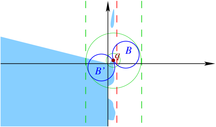
Figure 3.1. The geometry involved in the proof of Proposition 3.1.

Proof.

We let $\vartheta\in(-1,1)$ and $P_{t}=(t,\vartheta)\in\mathbb{R}^{2}$. We observe that if $t\geqslant 2$ then

$$B_{1}(P_{t}) \subseteq (t-1,t+1)\times(-2,2)$$

$$\subseteq \{x_{1}>1\},$$

and therefore, by (3.3),

$$B_{1}(P_{t})\cap E\cap{\mathcal{Q}}_{M,M}\subseteq\{x_{1}>1\}\cap\{x_{1}\in(0,\mu)\}=\varnothing.$$

We now take

$$t_{\star}:=\inf\left\{t\in\left[1,\frac{M}{8}\right]{\mbox{ s.t. }}B_{1}(P_{t})\cap E\cap{\mathcal{Q}}_{M,M}=\varnothing\right\}.$$

We claim that

$$t_{\star}=1.$$ (3.5)

To prove this, we argue by contradiction. If not, there exist $t_{\star}\in\left(1,\frac{M}{8}\right]$ and $q\in\big{(}\partial B_{1}(P_{t_{\star}})\big{)}\cap(\partial E)$, with $B:=B_{1}(P_{t_{\star}})\subseteq E^{c}$.

We remark that the first coordinate of $P_{t_{\star}}$ is equal to $t_{\star}$, and therefore

$$q_{1}\geqslant t_{\star}-1>0,$$ (3.6)

and also

$$q_{1}\leqslant t_{\star}+1\leqslant 1+\frac{M}{8}.$$ (3.7)

Similarly, we see that

$$|q_{2}|\leqslant 2.$$ (3.8)

We let $\nu$ be the exterior normal to $B$ at $q$ and $B^{\prime}:=B_{1}(P_{t_{\star}}+2\nu)$. We observe that $B^{\prime}$ is the symmetric ball to $B$ with respect to the tangent plane through $q$, see Figure 3.1. As a consequence, taking $\rho:=\sqrt[3]{\mu}$, since $B_{\rho}(q)\cap E\subseteq B^{c}$,

$$\int_{B_{\rho}(q)}\frac{\tilde{\chi}_{E}(x)}{|x-q|^{2+s}}dx\geqslant-\int_{B_{\rho}(q)\setminus(B\cup B^{\prime})}\frac{dx}{|x-q|^{2+s}}\geqslant-C\rho^{1-s}=-C\mu^{\frac{1-s}{3}},$$ (3.9)

for some $C>0$.

Now, we let

$$A_{1}:=\big{(}B_{1}(q)\setminus B_{\rho}(q)\big{)}\cap\{|x_{1}-q_{1}|\leqslant 2\mu\}$$

and $$A_{2}:=\big{(}B_{1}(q)\setminus B_{\rho}(q)\big{)}\cap\{|x_{1}-q_{1}|>2\mu\}.$$

We observe that

$$\int_{A_{1}}\frac{\tilde{\chi}_{E}(x)}{|x-q|^{2+s}}dx\geqslant-\int_{B_{1}(q)\cap\{|x_{1}-q_{1}|\leqslant 2\mu\}}\frac{dx}{\rho^{2+s}}\geqslant-\frac{C\mu}{\rho^{2+s}}=-C\mu^{\frac{1-s}{3}}.$$ (3.10)

Now we let

$${\mathcal{Q}}^{\star}:=(q_{1}-1,q_{1}+1)\times\left(-\frac{M}{4},\frac{M}{4}\right),$$

and we claim that

$$E\cap\big{(}{\mathcal{Q}}^{\star}\setminus B_{\rho}(q)\big{)}\cap\{x_{1}-q_{1}>2\mu\}=\varnothing.$$ (3.11)

Suppose not and let $p$ be in this set. Then, by (3.6),

$$p_{1}>2\mu+q_{1}>2\mu.$$

Similarly, by (3.7),

$$p_{1}<q_{1}+1\leqslant 2+\frac{M}{8}<M,$$

as long as $M$ is large enough. On the other hand, by (3.8),

$$|p_{2}|\leqslant|p_{2}-q_{2}|+|q_{2}|\leqslant\frac{M}{4}+2<M,$$

as long as $M$ is large enough. These observations give that

$$p\in E\cap{\mathcal{Q}}_{M,M}\cap\{x_{1}>2\mu\},$$

which is in contradiction with (3.3), and hence it proves (3.11).

Then, from (3.11) we deduce that

$$E\cap A_{2}\subseteq\{x_{1}-q_{1}<-2\mu\},$$

and consequently

$$\int_{A_{2}}\frac{\tilde{\chi}_{E}(x)}{|x-q|^{2+s}}dx\geqslant 0.$$

Then, combining this inequality with (3.10), we conclude that

$$\int_{B_{1}(q)\setminus B_{\rho}(q)}\frac{\tilde{\chi}_{E}(x)}{|x-q|^{2+s}}dx\geqslant-C\mu^{\frac{1-s}{3}}.$$

This and (3.9) yield that

$$\int_{B_{1}(q)}\frac{\tilde{\chi}_{E}(x)}{|x-q|^{2+s}}dx\geqslant-C\mu^{\frac{1-s}{3}},$$ (3.12)

up to renaming $C$.

Furthermore, by (3.11),

$$\int_{{\mathcal{Q}}^{\star}\setminus B_{1}(q)}\frac{\tilde{\chi}_{E}(x)}{|x-q|^{2+s}}dx\geqslant 0,$$

and therefore

$$\int_{\{|x_{1}-q_{1}|<1\}\setminus B_{1}(q)}\frac{\tilde{\chi}_{E}(x)}{|x-q|^{2+s}}dx\geqslant-\int_{\mathbb{R}^{2}\setminus B_{M/8}(q)}\frac{dx}{|x-q|^{2+s}}\geqslant-\frac{C}{M^{s}}.$$ (3.13)

Now, we observe that

$$E\cap\left\{x_{1}-q_{1}>1\right\}\subseteq\mathbb{R}^{2}\setminus B_{M/8}(q).$$ (3.14)

Indeed, if not, recalling (3.6), (3.7) and (3.8) we see that there exists $p=(p_{1},p_{2})\in E$ with

$$p_{1}<q_{1}+\frac{M}{8}\leqslant 1+\frac{M}{8}+\frac{M}{8}<M,$$

$$p_{1}>q_{1}+1>1>\mu,$$

$$|p_{2}|\leqslant|p_{2}-q_{2}|+|q_{2}|<\frac{M}{8}+1+\frac{M}{8}<M,$$

and these inequalities produce a contradiction with (3.3), thus proving (3.14).

Then, by (3.2) and (3.14),

$$\int_{B_{M/8}(q)\cap\{|x_{1}-q_{1}|>1\}}\frac{\tilde{\chi}_{E}(x)}{|x-q|^{2+s}}dx\geqslant c,$$

for some $c>0$, and, as a consequence,

$$\begin{split}&\int_{\{|x_{1}-q_{1}|>1\}\setminus B_{1}(q)}\frac{\tilde{\chi}_{E}(x)}{|x-q|^{2+s}}dx=\int_{\{|x_{1}-q_{1}|>1\}}\frac{\tilde{\chi}_{E}(x)}{|x-q|^{2+s}}dx\\ &\qquad\qquad\geqslant c-\int_{\mathbb{R}^{2}\setminus B_{M/8}(q)}\frac{dx}{|x-q|^{2+s}}\geqslant c-\frac{C}{M^{s}},\end{split}$$

for some $C>0$. This and (3.13) give that

$$\int_{\mathbb{R}^{2}\setminus B_{1}(q)}\frac{\tilde{\chi}_{E}(x)}{|x-q|^{2+s}}dx\geqslant c-\frac{C}{M^{s}},$$

up to renaming $C$, which, combined with (3.12), yields that

$$\int_{\mathbb{R}^{2}}\frac{\tilde{\chi}_{E}(x)}{|x-q|^{2+s}}dx\geqslant c-\frac{C}{M^{s}}-C\mu^{\frac{1-s}{3}}.$$

The latter quantity is strictly positive if $M$ is sufficiently large and $\mu$ is sufficiently small, which is in contradiction with the $s$-minimality of $E$.

This completes the proof of (3.5). Then, by (3.5), we obtain that

$$\varnothing=\bigcup_{t\geqslant 1}B_{1}(P_{t})\cap E\cap{\mathcal{Q}}_{M,M}\supseteq(\mathbb{R}\times\{\vartheta\})\cap E\cap{\mathcal{Q}}_{M,M},$$

from which (3.4) plainly follows since $\vartheta\in(-1,1)$ is arbitrary. ∎

As a consequence of Proposition 3.1, we have that $s$-minimal sets which approach empty sets in the halfspace are necessarily locally empty:

Corollary 3.2.

There exists $M_{0}>1$ such that the following claim holds true. Let $\varepsilon_{k}$ be an infinitesimal sequence. Let $\lambda>0$ and $E_{k}$ be a sequence of $s$-minimal sets in ${\mathcal{Q}}_{\frac{1}{\varepsilon_{k}},\frac{1}{\varepsilon_{k}}}$ such that

$$E_{k}\cap\{x_{1}<0\}\subseteq\{x_{2}\leqslant-\lambda x_{1}\}.$$

Assume that, for every $M\geqslant M_{0}$,

$$\chi_{E_{k}}\to 0 L^{1}\left(\left(\frac{1}{2M},2M\right)\times(-2M,2M)\right)$$ in . (3.15)

Then, for every $M\geqslant M_{0}$ there exists $k_{M}\in\mathbb{N}$ such that if $k\geqslant k_{M}$ then

$$E_{k}\cap{\mathcal{Q}}_{M,1}=\varnothing.$$

Proof.

Fix $M>0$, to be taken sufficiently large in what follows. First of all, we prove that, if $k$ is large enough, then

$$E_{k}\cap{\mathcal{Q}}_{M,M}\subseteq\left\{x_{1}\in\left(0,\frac{1}{M}\right)\right\}.$$ (3.16)

Suppose not. Then there are infinitely many values of $k$ for which there exists a point $p_{k}=(p_{k1},p_{k2})\in E_{k}$ with $p_{k1}\in\left[\frac{1}{M},M\right]$ and $|p_{k2}|\leqslant M$. We let $r:=\frac{1}{10\,M}$ and we claim that there exists $q_{k}\in B_{2r}(p_{k})$ and a constant $c\in\left(0,\frac{1}{2}\right)$ such that

$$B_{cr}(q_{k})\subseteq E_{k}.$$ (3.17)

Indeed, if $B_{r/2}(p_{k})\subseteq E_{k}$, then (3.17) holds true with $q_{k}:=p_{k}$. If instead $B_{r/2}(p_{k})\cap E_{k}\neq\varnothing$, there exists a point $z_{k}=(z_{k1},z_{k2})\in B_{r/2}(p_{k})\cap(\partial E_{k})$. We notice that if $\zeta=(\zeta_{1},\zeta_{2})\in B_{r}(z_{k})$ then

$$\zeta_{1}\geqslant z_{k1}-r\geqslant p_{k1}-\frac{3r}{2}\geqslant\frac{1}{M}-\frac{3r}{2}=\frac{17}{20\,M}>\varepsilon_{k}$$

and $$|\zeta_{i}|\leqslant|z_{ki}|+r\leqslant|p_{ki}|+\frac{3r}{2}\leqslant M+\frac{3}{20\,M}<\frac{1}{\varepsilon_{k}}$$

for all $i\in\{1,2\}$, which implies that $B_{r}(z_{k})\subseteq{\mathcal{Q}}_{\frac{1}{\varepsilon_{k}},\frac{1}{\varepsilon_{k}}}$, and therefore we can use the clean ball condition in [MR2675483] and conclude the proof of (3.17).

Moreover, up to a subsequence, we can assume that $p_{k}\to p$, for some $p\in\left[\frac{1}{M},M\right]\times[-M,M]$, and we observe that $B_{4r}(p)\supseteq B_{cr}(q_{k})$ if $k$ is sufficiently large. Accordingly, by (3.17), we find that

$$\int_{B_{4r}(p)}\chi_{E_{k}}(x)\,dx\geqslant\int_{B_{cr}(q_{k})}\chi_{E_{k}}(x)\,dx=|B_{cr}(q_{k})|=c^{\prime}\,r^{n},$$

for some $c^{\prime}>0$, which is in contradiction with (3.15), and hence it proves (3.16).

In light of (3.16), we have that $E_{k}$ satisfies the assumptions of Proposition 3.1. Consequently, the desired result follows from (3.4), up to renaming $M$. ∎

4. Alternative on the second blow-up

In this section, we analyze the $s$-minimal cone arising from the second blow-up, as described in Lemma 2.2, and we give a sharp alternative for its behavior. Roughly speaking, the alternative is that either a given $s$-minimal set exhibits the stickiness phenomenon or its second blow-up is a half-plane.

To state this result precisely, we say that a set $A$ is trivial in $B$ if either $A\cap B=B$ or $A\cap B=\varnothing$. Then, we have:

Theorem 4.1.

Let $\Omega:=(0,1)\times\mathbb{R}$. Let $E$ be an $s$-minimal graph in $\Omega$. Suppose that the boundary of $E$ meets the boundary of $\Omega$ at the origin and it is $C^{1}$ near the origin from outside $\Omega$.

Let $E_{00}$ be the second blow-up cone, as given in Lemma 2.2. Then the following alternative holds true:

• either $E_{00}$ is a halfplane,

• or there exists $r>0$ such that $E$ is trivial in $(0,r)\times(-r,r)$.

Proof.

From Lemma 2.2, it follows that $E_{00}$ has a graphical structure in the sense that if $p=(p_{1},p_{2})\in E_{00}$ then $(p_{1},\tau)\in E_{00}$ for all $\tau\leqslant p_{2}$ (actually, a similar statement also holds for $E_{0}$, using instead Lemma 2.1, but we focus here on $E_{00}$).

In the notation of (3.1), we claim that

if $$E_{00} \{x_{1}>0\} r>0 E {\mathcal{Q}}_{r,r}$$ is trivial in , then there exists  such that  is trivial in . (4.1)

To prove this, let us assume that

$$E_{00}\cap\{x_{1}>0\}=\varnothing$$

(the case $E_{00}\cap\{x_{1}>0\}=\{x_{1}>0\}$ can be treated similarly). By Lemma 2.3, we have that $\chi_{E_{k}}\to\chi_{E_{00}}=0$ in $L^{1}_{\rm loc}((0,+\infty)\times\mathbb{R})$, up to a subsequence (and, in fact, locally in the Hausdorff distance, thanks to Corollary C.2). Hence, we can exploit Corollary 3.2 with $M:=1$, and find that

$$E_{k}\cap{\mathcal{Q}}_{1,1}=\varnothing,$$

as long as $k$ is sufficiently large. We can thereby conclude that

$$E\cap{\mathcal{Q}}_{\frac{1}{k},\frac{1}{k}}=\varnothing,$$

which completes the proof of (4.1).

Now, to complete the proof of Theorem 4.1, we suppose that $E$ is not trivial in ${\mathcal{Q}}_{r,r}$: then the desired claim in Theorem 4.1 is established if we show that $E_{00}$ is a half-plane. To this end, we know from (4.1) that $E_{00}$ cannot be trivial in $\{x_{1}>0\}$. Consequently, since $E_{00}$ is a cone, in light of Lemma 2.2, we can write that

$$E_{00}\cap\{x_{1}<0\}=\{x_{2}<ax_{1}\}\qquad{\mbox{ and }}\qquad E_{00}\cap\{x_{1}>0\}=\{x_{2}<bx_{1}\},$$

for some $a$, $b\in\mathbb{R}$. We claim that

$$a=b.$$ (4.2)

Indeed, suppose not. Then, we compute the nonlocal mean curvature equation at the point $p:=(1,b)\in\partial E_{00}$, symmetrizing the integral with respect to the line $\{x_{2}=bx_{1}\}$ and we obtain that

$$\int_{\mathbb{R}^{2}}\frac{\chi_{\mathbb{R}^{2}\setminus E_{00}}(p)-\chi_{E_{00}}(p)}{|x-p|^{2+s}}\,dx\neq 0.$$

This is a contradiction with the minimality of $E_{00}$, and hence it proves (4.2), thus completing the proof of Theorem 4.1. ∎

From the blow-up alternative in Theorem 4.1, we obtain that an $s$-minimal graph cannot develop boundary corners, unless it develops boundary stickiness (that is, no “nude” Lipschitz singularity is possible, since any corner would naturally produce boundary discontinuities). The precise result that we have is the following:

Corollary 4.2.

Let $\Omega:=(0,1)\times\mathbb{R}$. Let $E$ be a locally $s$-minimal graph in $\Omega$. Suppose that the boundary of $E$ meets the boundary of $\Omega$ at the origin and it is $C^{1}$ near the origin from outside $\Omega$. Assume also that the tangent line of $\partial E$ from outside $\Omega$ is of the form $x_{2}=\ell x_{1}$, with $\ell\in\mathbb{R}$.

Then:

• if

  $$\{x\in\mathbb{R}^{2}{\mbox{ s.t. }}x_{1}\in(0,\delta){\mbox{ and }}x_{2}<(\ell+\delta)x_{1}\}\subseteq E$$ (4.3)

  for some $\delta>0$, then there exists $\delta^{\prime}>0$ such that $(0,\delta^{\prime})^{2}\subseteq E$;

• if

  $$\{x\in\mathbb{R}^{2}{\mbox{ s.t. }}x_{1}\in(0,\delta){\mbox{ and }}x_{2}<(\ell-\delta)x_{1}\}\supseteq E$$

  for some $\delta>0$, then there exists $\delta^{\prime}>0$ such that $(0,\delta^{\prime})\times(-\delta^{\prime},0)\subseteq\mathbb{R}^{2}\setminus E$.

Proof.

We prove the first claim of Corollary 4.2, since the second one would then follow by considering complementary sets. If (4.3) is satisfied, then the second blow-up $E_{00}$ in Lemma 2.2 would satisfy

$$E_{00}\cap\{x_{1}<0\}=\{x_{2}<\ell x_{1}\}\cap\{x_{1}<0\}$$

and $$E_{00}\cap\{x_{1}>0\}\supseteq\{x_{2}<(\ell+\delta)x_{1}\}\cap\{x_{1}>0\}.$$

In particular, $E_{00}$ is not a half-plane, and hence the claim follows from Theorem 4.1. ∎

It is interesting to notice that the boundary behavior described in Corollary 4.2 is significantly different not only with respect to the case of classical minimal surfaces, but also with respect to the case of nonlocal capillarity problems. Indeed, in the nonlocal capillarity theory the minimizers satisfy uniform density estimates at the boundary, as proved in Theorem 1.7 of [MR3717439]: instead, the minimizers of the nonlocal perimeters do not possess similar boundary density estimates in the domain, exactly in view of the stickiness phenomenon. In a sense, as we will also see in the forthcoming section and in Appendix C, the role of this density estimates in our setting will be recovered by the mass of the set and of its complement which arises from the exterior datum.

5. Boundary Harnack Inequality

The main goal of this section is to provide a suitable Harnack Inequality for $E$ “up to the boundary”. The results obtained will then complement those in Section 6.3 of [MR2675483], where similar results where obtained in the interior of the domain. Interestingly, the boundary Harnack inequality is stronger than the one in the interior, since one is able to decrease the oscillation both from above and from below. More precisely, the main result of this section is the following:

Lemma 5.1.

Let $\alpha\in(0,s)$, $\ell\in\mathbb{R}$, $u:\mathbb{R}\to\mathbb{R}$ and

$$E:=\{(x_{1},x_{2})\in\mathbb{R}^{2}{\mbox{ s.t. }}x_{2}<u(x_{1})\}.$$

Assume that $E$ is locally $s$-minimal in $(0,1)\times\mathbb{R}$. Then, there exist $\eta\in(0,1)$, $\delta\in(0,1)$ and $\varepsilon_{0}\in(0,\min\{\eta,\delta\})$, depending only on $\alpha$, $\ell$, and $s$, such that if $\varepsilon\in(0,\varepsilon_{0})$ the following statement holds true.

Let

$$k_{0}:=\left\lceil\frac{-\log_{2}\varepsilon}{\alpha}\right\rceil,$$ (5.1)

and suppose that

$$|u(x_{1})-\ell x_{1}|\leqslant\delta\varepsilon(2^{k})^{1+\alpha}{\mbox{ for all $x_{1}\in(-2^{k},0)$, for all $k\in\{0,\dots,k_{0}\}$,}}$$ (5.2)

$$|u(x_{1})-\ell x_{1}|\leqslant\varepsilon(2^{k})^{1+\alpha}{\mbox{ for all $x_{1}\in(0,2^{k})$, for all $k\in\{0,\dots,k_{0}\}$.}}$$ (5.3)

Then,

$$\sup_{x_{1}\in(0,\eta)}u(x_{1})-\ell x_{1}\leqslant\varepsilon(1-\eta^{2}),$$ (5.4)

and $$\inf_{x_{1}\in(0,\eta)}u(x_{1})-\ell x_{1}\geqslant\varepsilon(\eta^{2}-1).$$ (5.5)

Proof.

We use the sliding method of Lemma 6.9 of [MR2675483], by taking into account the following complications. First of all, we do not impose a priori that the touching points occur in the interior. Secondly, the sliding parabola is adapted to take into consideration the linear perturbation provided by the parameter $\ell$. On the other hand, dealing with these two complications will produce an interesting byproduct since the Harnack inequality that we obtain establishes both the oscillation improvement from above in (5.4) and the one from below in (5.5) (while in the interior case one can only prove either one or the other): in our situation, this additional information will be a consequence of the regularity of the data outside the domain, which, in view of (5.2) produces exterior mass of both the set and of its complement.

The details go as follows. We prove that (5.5) holds true (the proof of (5.4) is similar). We argue by contradiction, supposing that (5.5) is violated, hence there exists $t_{\star}\in(0,\eta)$ with

$$u(t_{\star})-\ell t_{\star}<\varepsilon(\eta^{2}-1).$$ (5.6)

We let

$${\mathcal{C}}:=\{x=(x_{1},x_{2})\in\mathbb{R}^{2}{\mbox{ s.t. }}x_{1}\in(-\eta,\eta){\mbox{ and }}|x_{2}-\ell x_{1}|<\varepsilon\}.$$

We prove that

$$|E\cap{\mathcal{C}}|\geqslant\frac{\varepsilon\eta}{2}.$$ (5.7)

This will be established once we show that

$$\left\{x=(x_{1},x_{2})\in\mathbb{R}^{2}{\mbox{ s.t. }}x_{1}\in(-\eta,0){\mbox{ and }}x_{2}\in\left(u(x_{1})-\frac{\varepsilon}{2},u(x_{1})\right)\right\}\subseteq E\cap{\mathcal{C}}.$$ (5.8)

To prove this claim, let $x$ be in the set on the left hand side of (5.8). Then, we have that $x_{2}<u(x_{1})$, and thus $x\in E$. Moreover, using (5.2) with $k:=0$,

$$|x_{2}-\ell x_{1}|\leqslant|x_{2}-u(x_{1})|+|u(x_{1})-\ell x_{1}|\leqslant\frac{\varepsilon}{2}+\delta\varepsilon<\varepsilon,$$

as long as $\delta<\frac{1}{2}$, and consequently $x\in{\mathcal{C}}$. This proves (5.8), and hence (5.7) readily follows.

Now, by varying the parameter $\kappa\in\mathbb{R}$, we slide by below a parabola ${\mathcal{P}}_{\kappa}$ of the form

$$x_{2}=\ell x_{1}-\frac{\varepsilon(x_{1}-t_{\star})^{2}}{2}-\kappa$$

till it touches $u$ in $\{|x_{1}|\leqslant 1\}$.

To formalize this idea, we first observe that, by (5.2) and (5.3) (used here with $k:=0$), if $|x_{1}|\leqslant 1$,

$$\ell x_{1}-\frac{\varepsilon(x_{1}-t_{\star})^{2}}{2}-\kappa-u(x_{1})\leqslant\varepsilon-\frac{\varepsilon(x_{1}-t_{\star})^{2}}{2}-\kappa\leqslant\varepsilon-\kappa,$$

and so if $\kappa\geqslant 1$, we have that ${\mathcal{P}}_{\kappa}$ lies below the graph of $u$ in $\{|x_{1}|\leqslant 1\}$.

Then, we can take $\kappa$ as small as possible with this property. We observe that, for this choice of $\kappa$,

there must be an interior touching point in $$\{x_{1}\in(0,5\eta)\}$$. (5.9)

Indeed, by (5.6) and the fact that $u$ lies above the parabola ${\mathcal{P}}_{\kappa}$,

$$0\geqslant\ell t_{\star}-\kappa-u(t_{\star})>-\kappa-\varepsilon(\eta^{2}-1),$$

which gives that

$$\kappa>\varepsilon(1-\eta^{2}).$$ (5.10)

Hence, if $x_{1}\in(-1,0)$, by (5.2) we have that

$$\ell x_{1}-\frac{\varepsilon(x_{1}-t_{\star})^{2}}{2}-\kappa-u(x_{1})<\delta\varepsilon-\frac{\varepsilon(x_{1}-t_{\star})^{2}}{2}-\varepsilon(1-\eta^{2})\leqslant-\varepsilon\left(1-\eta^{2}-\delta\right)\leqslant-\frac{\varepsilon}{2},$$

as long as $\eta$ and $\delta$ are sufficiently small, which says that

the parabola is well separated by $$u \{x_{1}\in(-1,0)\}$$ in . (5.11)

Furthermore, if $x_{1}\in[5\eta,1]$, we have that $x_{1}-t_{\star}\geqslant 4\eta$ and then, by (5.3) and (5.10),

$$\ell x_{1}-\frac{\varepsilon(x_{1}-t_{\star})^{2}}{2}-\kappa-u(x_{1})\leqslant\varepsilon-\frac{\varepsilon(x_{1}-t_{\star})^{2}}{2}-\kappa<\varepsilon-\frac{\varepsilon(x_{1}-t_{\star})^{2}}{2}-\varepsilon(1-\eta^{2})$$

$$\qquad\leqslant\varepsilon-8\varepsilon\eta^{2}-\varepsilon(1-\eta^{2})=-7\varepsilon\eta^{2},$$

hence the parabola is well separated by $u$ in $\{x_{1}\in[5\eta,1]\}$.

From this and (5.11) we obtain that the parabola touches the graph of $u$ at some point in $[0,5\eta)$. To complete the proof of (5.9), we have to check that

this touching point cannot occur at $$x_{1}=0$$. (5.12)

We argue by contradiction, assuming that this is the case. Then, recalling (5.11),

$$-\frac{\varepsilon t_{\star}^{2}}{2}-\kappa=\liminf_{x_{1}\searrow 0}u(x_{1})<\liminf_{x_{1}\nearrow 0}u(x_{1}).$$

That is, the $s$-minimal surface $E$ would have a boundary point $P=(P_{1},P_{2}):=\left(0,-\frac{\varepsilon t_{\star}^{2}}{2}-\kappa\right)$ such that $B_{\rho}(P)\setminus\Omega\subset E$, as long as $\rho>0$ is small enough.

By this and Theorem 1.1 in [MR3532394], it follows that, near $P$, the boundary of $E$ can be written as a $C^{1,\frac{1+s}{2}}$-graph in the horizontal direction, namely

$$\partial E\cap B_{\rho^{\prime}}(P)=\{x\in\mathbb{R}{\mbox{ s.t. }}x_{1}=\phi(x_{2})\}\cap B_{\rho^{\prime}}(P),$$

for some $\rho^{\prime}>0$ and $\phi\in C^{1,\frac{1+s}{2}}(\mathbb{R})$, with $\phi(P_{2})=P_{1}=0$ and $\phi^{\prime}(P_{2})=0$. By construction, we have that $u(\phi(x_{2}))=x_{2}$, for $x_{2}$ close to $P_{2}$, and hence, the condition that the parabola ${\mathcal{P}}_{\kappa}$ lies below $u$ (with equality at $x_{1}=0$) gives that

$$x_{2}\geqslant\ell\phi(x_{2})-\frac{\varepsilon(\phi(x_{2})-t_{\star})^{2}}{2}-\kappa,$$

as long as $x_{2}$ is close enough to $P_{2}$ (with equality at $x_{2}=P_{2}$). As a consequence,

$$0 \geqslant \left(\ell\phi(x_{2})-\frac{\varepsilon(\phi(x_{2})-t_{\star})^{2}}{2}-\kappa-x_{2}\right)-\left(\ell\phi(P_{2})-\frac{\varepsilon(\phi(P_{2})-t_{\star})^{2}}{2}-\kappa-P_{2}\right)$$

$$= \ell\phi(x_{2})+\frac{\varepsilon}{2}\Big{(}t_{\star}^{2}-(\phi(x_{2})-t_{\star})^{2}\Big{)}+P_{2}-x_{2}$$

$$= \ell\phi(x_{2})+\frac{\varepsilon}{2}\Big{(}2t_{\star}\phi(x_{2})-\phi^{2}(x_{2})\Big{)}+P_{2}-x_{2}$$

$$= \left(\ell+\frac{\varepsilon}{2}\Big{(}2t_{\star}-\phi(x_{2})\Big{)}\right)\phi(x_{2})+P_{2}-x_{2}$$

and thus

$$1\leqslant\lim_{x_{2}\to P_{2}}\left(\ell+\frac{\varepsilon}{2}\Big{(}2t_{\star}-\phi(x_{2})\Big{)}\right)\frac{\phi(x_{2})}{x_{2}-P_{2}}=\left(\ell+\varepsilon t_{\star}\right)\,\phi^{\prime}(P_{2})=0.$$

This contradiction completes the proof of (5.12), and hence of (5.9), as desired.

Then, by (5.9), there exists $Q\in(\partial E)\cap\{x_{1}\in(0,5\eta)\}$ which is touched from below by the parabola ${\mathcal{P}}_{\kappa}$.

We denote by $\underline{\mathcal{P}}_{\kappa}$ the subgraph of ${\mathcal{P}}_{\kappa}$, and we observe that most of $\underline{\mathcal{P}}_{\kappa}$ lies outside ${\mathcal{C}}$. More explicitly, we claim that

$$|\underline{\mathcal{P}}_{\kappa}\cap{\mathcal{C}}|\leqslant C(\ell)\,\varepsilon\eta^{3}.$$ (5.13)

for some $C(\ell)>0$. Indeed, if $x$ belongs to $\underline{\mathcal{P}}_{\kappa}\cap{\mathcal{C}}$ we have that $|x_{1}|<\eta$, $|x_{2}-\ell x_{1}|<\varepsilon$ and

$$x_{2}<\ell x_{1}-\frac{\varepsilon(x_{1}-t_{\star})^{2}}{2}-\kappa.$$

Consequently, recalling (5.10),

$$x_{2}-\ell x_{1}<-\kappa<-\varepsilon(1-\eta^{2})=-\varepsilon+\varepsilon\eta^{2}.$$

These observations say that $\underline{\mathcal{P}}_{\kappa}\cap{\mathcal{C}}$ is contained in the parallelogram

$$\{x\in\mathbb{R}^{2}{\mbox{ s.t. }}x_{1}\in(-\eta,\eta){\mbox{ and }}x_{2}-\ell x_{1}\in(-\varepsilon,-\varepsilon+\varepsilon\eta^{2})\},$$

which in turn implies (5.13).

Assuming $\eta$ sufficiently small, we deduce from (5.7) and (5.13) that

$$\big{|}(E\cap{\mathcal{C}})\setminus\underline{\mathcal{P}}_{\kappa}\big{|}\geqslant\frac{\varepsilon\eta}{4}.$$ (5.14)

We also observe that

$${\mathcal{C}}\subseteq B_{C_{0}(\ell)\eta}(Q)$$ (5.15)

for some $C_{0}(\ell)>0$. Indeed, if $y\in{\mathcal{C}}$, we have that $|y_{1}-Q_{1}|\leqslant 6\eta$ and

$$|y_{2}-Q_{2}|\leqslant|y_{2}-\ell y_{1}|+|\ell|\,|y_{1}-Q_{1}|+|\ell Q_{1}-Q_{2}|\leqslant\varepsilon+6|\ell|\,\eta+|\ell Q_{1}-u(Q_{1})|\leqslant 2\varepsilon+6|\ell|\,\eta,$$

where (5.3) was used once again in the last step, and accordingly $|y-Q|\leqslant C_{0}(\ell)\eta$, for some $C_{0}(\ell)>0$, as long as $\varepsilon$ is small enough.

This proves (5.15). In particular, if $\eta$ is sufficiently small, we conclude that ${\mathcal{C}}\subseteq B_{1/2}(Q)$. In addition, we observe that $\underline{\mathcal{P}}_{\kappa}$ at $Q$ has curvature $-\frac{\varepsilon}{(1+\ell^{2})^{\frac{3}{2}}}+O(\varepsilon^{2})$, and therefore

$$\begin{split}&\int_{B_{1/2}(Q)}\frac{\chi_{\mathbb{R}^{2}\setminus E}(y)-\chi_{E}(y)}{|y-Q|^{2+s}}\,dy\\ =\;&-\int_{B_{1/2}(Q)\cap\underline{\mathcal{P}}_{\kappa}}\frac{dy}{|y-Q|^{2+s}}+\int_{B_{1/2}(Q)\setminus\underline{\mathcal{P}}_{\kappa}}\frac{\chi_{\mathbb{R}^{2}\setminus E}(y)-\chi_{E}(y)}{|y-Q|^{2+s}}\,dy\\ =\;&-\int_{B_{1/2}(Q)\cap\underline{\mathcal{P}}_{\kappa}}\frac{dy}{|y-Q|^{2+s}}+\int_{(E^{c}\cap B_{1/2}(Q))\setminus\underline{\mathcal{P}}_{\kappa}}\frac{dy}{|y-Q|^{2+s}}-\int_{(E\cap B_{1/2}(Q))\setminus\underline{\mathcal{P}}_{\kappa}}\frac{dy}{|y-Q|^{2+s}}\\ \leqslant\;&C_{1}(\ell)\varepsilon-\int_{(E\cap B_{1/2}(Q))\setminus\underline{\mathcal{P}}_{\kappa}}\frac{dy}{|y-Q|^{2+s}}\\ \leqslant\;&C_{1}(\ell)\varepsilon-\int_{(E\cap{\mathcal{C}})\setminus\underline{\mathcal{P}}_{\kappa}}\frac{dy}{|y-Q|^{2+s}},\end{split}$$

for some $C_{1}(\ell)>0$. Therefore, using again (5.15), we conclude that

$$\int_{B_{1/2}(Q)}\frac{\chi_{\mathbb{R}^{2}\setminus E}(y)-\chi_{E}(y)}{|y-Q|^{2+s}}\,dy\leqslant C_{1}(\ell)\varepsilon-\frac{\big{|}(E\cap{\mathcal{C}})\setminus\underline{\mathcal{P}}_{\kappa}\big{|}}{(C_{0}(\ell)\eta)^{2+s}}.$$

This and (5.14) give that

$$\int_{B_{1/2}(Q)}\frac{\chi_{\mathbb{R}^{2}\setminus E}(y)-\chi_{E}(y)}{|y-Q|^{2+s}}\,dy\leqslant-\frac{C_{2}(\ell)\,\varepsilon}{\eta^{1+s}}+C_{1}(\ell)\varepsilon,$$ (5.16)

for some $C_{2}(\ell)>0$.

Furthermore, by (5.2) and (5.3),

$$\int_{B_{2^{k_{0}-1}}(Q)\setminus B_{1/2}(Q)}\frac{\chi_{\mathbb{R}^{2}\setminus E}(y)-\chi_{E}(y)}{|y-Q|^{2+s}}\,dy\leqslant C\varepsilon\int_{1/2}^{2^{k_{0}}}t^{\alpha-1-s}\,dt\leqslant\frac{C\varepsilon}{s-\alpha},$$ (5.17)

for some $C>0$.

In addition, by (5.1),

$$\int_{\mathbb{R}^{2}\setminus B_{2^{k_{0}-1}}(Q)}\frac{\chi_{\mathbb{R}^{2}\setminus E}(y)-\chi_{E}(y)}{|y-Q|^{2+s}}\,dy\leqslant\frac{C^{\prime}}{s\,(2^{k_{0}-1})^{s}}\leqslant C(\alpha,s)\,\varepsilon,$$

for some $C^{\prime}$, $C(\alpha,s)>0$. Combining this, (5.16) and (5.17), we find that

$$\frac{1}{\varepsilon}\,\int_{\mathbb{R}^{2}}\frac{\chi_{\mathbb{R}^{2}\setminus E}(y)-\chi_{E}(y)}{|y-Q|^{2+s}}\,dy\leqslant-\frac{C_{2}(\ell)}{\eta^{1+s}}+C_{1}(\ell)+\frac{C}{s-\alpha}+C(\alpha,s),$$

which is strictly negative as long as $\eta$ is sufficiently small. This contradiction proves (5.5), as desired. ∎

As customary, Lemma 5.1 can be iterated (though a finite number of times for a fixed $\varepsilon$). In our setting, this iteration is somewhat more delicate than in the interior case, since one has to treat the data from outside differently from the solution from the inside and obtain uniform estimates at the boundary. The result that we obtain is therefore the following:

Corollary 5.2.

Let $\alpha\in(0,s)$, $\ell\in\mathbb{R}$, $u:\mathbb{R}\to\mathbb{R}$ and

$$E:=\{(x_{1},x_{2})\in\mathbb{R}^{2}{\mbox{ s.t. }}x_{2}<u(x_{1})\}.$$

Assume that $E$ is locally $s$-minimal in $(0,1)\times\mathbb{R}$. Then, there exist $c_{0}$, $\eta$, $\delta$ and $\tilde{\varepsilon}_{0}\in(0,1)$, depending only on $\alpha$, $\ell$, and $s$, such that if $\varepsilon\in(0,\tilde{\varepsilon}_{0})$ the following statement holds true.

Let

$$\tilde{k}_{0}:=\left\lceil\frac{-\log\varepsilon}{c_{0}}\right\rceil,$$ (5.18)

and suppose that

$$|u(x_{1})-\ell x_{1}|\leqslant\varepsilon^{\frac{1}{c_{0}}}\,|x_{1}|^{1+\alpha}{\mbox{ for all $x_{1}\in(-2^{\tilde{k}_{0}},0)$,}}$$ (5.19)

$$|u(x_{1})-\ell x_{1}|\leqslant\varepsilon(2^{k})^{1+\alpha}{\mbox{ for all $x_{1}\in(0,2^{k})$, for all $k\in\{0,\dots,\tilde{k}_{0}\}$.}}$$ (5.20)

Then, for every $m\in\mathbb{N}$ such that

$$1\leqslant m\leqslant c_{0}\,|\log\varepsilon|,$$ (5.21)

we have that

$$\sup_{x_{1}\in(-\eta^{m},\eta^{m})}|u(x_{1})-\ell x_{1}|\leqslant\varepsilon(1-\eta^{2})^{m}.$$ (5.22)

In particular, under assumptions (5.19) and (5.20), there exist $\vartheta_{1}$, $\vartheta_{2}\in(0,1)$ such that, for any $x_{1}\in(-\eta,\eta)$,

$$|u(x_{1})-\ell x_{1}|\leqslant\varepsilon\max\{x_{1}^{\vartheta_{1}},\,\varepsilon^{\vartheta_{2}}\}.$$ (5.23)

Proof.

We have that (5.23) readily follows from (5.21) and (5.22). Hence, we focus on the proof of (5.22).

To this end, we observe that, if $x_{1}\in(-\eta^{m},0)$ we can exploit (5.19) and see that

$$|u(x_{1})-\ell x_{1}|\leqslant\varepsilon^{\frac{1}{c_{0}}}\,\eta^{(1+\alpha)m}=\varepsilon^{\frac{1}{c_{0}}}(1-\eta^{2})^{m}\,\left(\frac{\eta^{1+\alpha}}{1-\eta^{2}}\right)^{m}\leqslant\varepsilon^{\frac{1}{c_{0}}}(1-\eta^{2})^{m},$$

which implies (5.22) in this case.

Consequently, to prove (5.22), it is enough to consider the case $x_{1}\in(0,\eta^{m})$.

Hence, we prove (5.22) when $x_{1}\in(0,\eta^{m})$ by induction over $m\in\mathbb{N}$. We let $\eta$, $\delta$ and $\varepsilon_{0}$ be as in Lemma 5.1 and we iterate such a result till

$$m\leqslant\frac{\log\frac{\varepsilon_{0}}{\varepsilon}}{\log\frac{1-\eta^{2}}{\eta}}.$$ (5.24)

We will also take $\tilde{\varepsilon}_{0}$ in the statement of Corollary 5.2 to be equal to $\varepsilon_{0}^{2}$. In this way, for every $\varepsilon\in(0,\tilde{\varepsilon}_{0})$, we have that

$$\log\frac{\varepsilon_{0}}{\varepsilon}=\frac{1}{2}\,\log\frac{\tilde{\varepsilon}_{0}}{\varepsilon^{2}}\geqslant\frac{1}{2}\,\log\frac{1}{\varepsilon},$$

and therefore (5.21) implies (5.24) for a suitable choice of $c_{0}$.

For future convenience, we also set

$$\tilde{C}(\eta):=-\frac{\log(1-\eta^{2})}{\log\frac{1-\eta^{2}}{\eta}}>0.$$ (5.25)

The induction argument goes as follows. First of all, up to taking $\eta$ in Lemma 5.1 smaller, we can assume that $\eta=2^{-M_{0}}$, for some $M_{0}\in\mathbb{N}$, $M_{0}\geqslant 2$. When $m=1$, we have that (5.22) follows from Lemma 5.1.

We now suppose that (5.22) holds true for all $m\in\{1,\dots,m_{0}\}$, with

$$m_{0}\leqslant\frac{\log\frac{\varepsilon_{0}}{\varepsilon}}{\log\frac{1-\eta^{2}}{\eta}},$$ (5.26)

and we want to prove that (5.22) holds true for $m=m_{0}+1$.

To this end, we define

$$\tilde{u}(x_{1}):=\frac{1}{\eta^{m_{0}}}\,u(\eta^{m_{0}}x_{1})\qquad{\mbox{ and }}\qquad\tilde{\varepsilon}:=\frac{\varepsilon(1-\eta^{2})^{m_{0}}}{\eta^{m_{0}}}.$$

We also use the notation

$$x_{1}:=\eta^{m_{0}}\tilde{x}_{1}\qquad{\mbox{ and }}k:=\tilde{k}-m_{0}M_{0}.$$ (5.27)

Then, we claim that

$$|\tilde{u}(\tilde{x}_{1})-\ell\tilde{x}_{1}|\leqslant\delta\tilde{\varepsilon}(2^{\tilde{k}})^{1+\alpha}{\mbox{ for all $\tilde{x}_{1}\in(-2^{\tilde{k}},0)$, for all $\tilde{k}\in\{0,\dots,\tilde{k}_{0}\}$.}}$$ (5.28)

For this, we exploit (5.19) and obtain that

$$|\tilde{u}(\tilde{x}_{1})-\ell\tilde{x}_{1}|=\frac{1}{\eta^{m_{0}}}|u(x_{1})-\ell x_{1}|\leqslant\frac{\varepsilon^{\frac{1}{c_{0}}}\,|x_{1}|^{1+\alpha}}{{\eta^{m_{0}}}}=\frac{\varepsilon^{\frac{1}{c_{0}}-1}\,\tilde{\varepsilon}\,|x_{1}|^{1+\alpha}}{{(1-\eta^{2})^{m_{0}}}}.$$ (5.29)

On the other hand, from (5.25) and (5.26),

$$\log\Big{(}(1-\eta^{2})^{m_{0}}\Big{)}=m_{0}\,\log(1-\eta^{2})\geqslant\frac{\log\frac{\varepsilon_{0}}{\varepsilon}\;\log(1-\eta^{2})}{\log\frac{1-\eta^{2}}{\eta}}$$

$$\qquad\qquad=-\tilde{C}(\eta)\,\log\frac{\varepsilon_{0}}{\varepsilon}=\log\frac{\varepsilon^{\tilde{C}(\eta)}}{\varepsilon_{0}^{\tilde{C}(\eta)}}\geqslant\log\big{(}\varepsilon^{\tilde{C}(\eta)}\big{)},$$

and therefore $(1-\eta^{2})^{m_{0}}\geqslant\varepsilon^{\tilde{C}(\eta)}$. Then, by plugging this information into (5.29), we conclude that

$$|\tilde{u}(\tilde{x}_{1})-\ell\tilde{x}_{1}|\leqslant\varepsilon^{\frac{1}{c_{0}}-1-\tilde{C}(\eta)}\,\tilde{\varepsilon}\,|x_{1}|^{1+\alpha}\leqslant\delta\tilde{\varepsilon}\,|x_{1}|^{1+\alpha},$$

provided that $c_{0}$ is chosen small enough, which gives (5.28), as desired.

Now we claim that

$$|\tilde{u}(\tilde{x}_{1})-\ell\tilde{x}_{1}|\leqslant\tilde{\varepsilon}(2^{\tilde{k}})^{1+\alpha}{\mbox{ for all $\tilde{x}_{1}\in(0,2^{\tilde{k}})$, for all $\tilde{k}\in\{0,\dots,\tilde{k}_{0}\}$.}}$$ (5.30)

To check this, we first consider the case $\tilde{k}\in\{0,\dots,m_{0}M_{0}\}$, and we let

$$m_{\tilde{k}}:=\left\lfloor m_{0}-\frac{\tilde{k}}{M_{0}}\right\rfloor\in\{0,\dots,m_{0}\}.$$

We point out that

$$x_{1}=2^{-m_{0}M_{0}}\tilde{x}_{1}\in(0,2^{-m_{0}M_{0}+\tilde{k}})\subseteq(0,2^{-M_{0}m_{\tilde{k}}})=(0,\eta^{m_{\tilde{k}}}).$$

Then, since we know by inductive assumption that (5.22) is satisfied when $m\leqslant m_{0}$, we find that

$$|\tilde{u}(\tilde{x}_{1})-\ell\tilde{x}_{1}|=\frac{1}{\eta^{m_{0}}}\,|u(x_{1})-\ell x_{1}|\leqslant\frac{\varepsilon(1-\eta^{2})^{m_{\tilde{k}}}}{\eta^{m_{0}}}.$$ (5.31)

Now, when $\tilde{k}=0$ we deduce from (5.31) that

$$|\tilde{u}(\tilde{x}_{1})-\ell\tilde{x}_{1}|\leqslant\frac{\varepsilon(1-\eta^{2})^{m_{0}}}{\eta^{m_{0}}}=\tilde{\varepsilon},$$

which is (5.30) in this case.

If instead $\tilde{k}\in\{1,\dots,m_{0}M_{0}\}$, we infer from (5.31) that

$$|\tilde{u}(\tilde{x}_{1})-\ell\tilde{x}_{1}|\leqslant\tilde{\varepsilon}(1-\eta^{2})^{m_{\tilde{k}}-m_{0}}=\tilde{\varepsilon}(2^{\tilde{k}})^{1+\alpha}\times\frac{(1-\eta^{2})^{m_{\tilde{k}}-m_{0}}}{2^{\tilde{k}(1+\alpha)}}.$$ (5.32)

Moreover,

$$(1-\eta^{2})^{\frac{1}{M_{0}}}\;2^{1+\alpha}=(1-2^{-2M_{0}})^{\frac{1}{M_{0}}}\;2^{1+\alpha}\geqslant 2^{\alpha},$$

as long as $\eta$ is small enough (hence $M_{0}$ large enough), and thus

$$\frac{(1-\eta^{2})^{m_{\tilde{k}}-m_{0}}}{2^{\tilde{k}(1+\alpha)}}\leqslant\frac{(1-\eta^{2})^{-\frac{\tilde{k}}{M_{0}}-1}}{2^{\tilde{k}(1+\alpha)}}=\frac{1}{1-\eta^{2}}\;\left(\frac{1}{(1-\eta^{2})^{\frac{1}{M_{0}}}\;2^{1+\alpha}}\right)^{\tilde{k}}$$

$$\qquad\qquad\leqslant\frac{1}{(1-\eta^{2})\;2^{\alpha\tilde{k}}}\leqslant\frac{1}{(1-\eta^{2})\;2^{\alpha}}\leqslant 1,$$

provided that $\eta$ is small enough.

From this and (5.32), we conclude that

$$|\tilde{u}(\tilde{x}_{1})-\ell\tilde{x}_{1}|\leqslant\tilde{\varepsilon}(2^{\tilde{k}})^{1+\alpha}.$$

The latter estimate gives (5.30) when $\tilde{k}\in\{1,\dots,m_{0}M_{0}\}$.

Now, we focus on the proof of (5.30) when $\tilde{k}\in\{m_{0}M_{0}+1,\dots,\tilde{k}_{0}\}$. In this case, we exploit (5.20) with the notation in (5.27), observing that $k\geqslant 0$ and $x_{1}\in(0,\eta^{m_{0}}2^{\tilde{k}})=(0,2^{k})$, and we conclude that

$$|\tilde{u}(\tilde{x}_{1})-\ell\tilde{x}_{1}|=\frac{1}{\eta^{m_{0}}}\,|u(x_{1})-\ell x_{1}|\leqslant\frac{\varepsilon(2^{k})^{1+\alpha}}{\eta^{m_{0}}}$$

$$\qquad=\tilde{\varepsilon}(2^{\tilde{k}})^{1+\alpha}\times\frac{(2^{-m_{0}M_{0}})^{1+\alpha}}{(1-\eta^{2})^{m_{0}}}=\tilde{\varepsilon}(2^{\tilde{k}})^{1+\alpha}\times\left(\frac{\eta^{1+\alpha}}{(1-\eta^{2})}\right)^{m_{0}}\leqslant\tilde{\varepsilon}(2^{\tilde{k}})^{1+\alpha}.$$

This gives (5.30) when $\tilde{k}\in\{m_{0}M_{0}+1,\dots,\tilde{k}_{0}\}$. The proof of (5.30) is therefore complete.

Now, by (5.28) and (5.30), we obtain that (5.2) and (5.3) are satisfied, with $\tilde{u}$ and $\tilde{\varepsilon}$ instead of $u$ and $\varepsilon$.

Also, in view of (5.26),

$$\tilde{\varepsilon}=\varepsilon\times\left(\frac{1-\eta^{2}}{\eta}\right)^{m_{0}}\leqslant\varepsilon\times\left(\frac{1-\eta^{2}}{\eta}\right)^{\frac{\log\frac{\varepsilon_{0}}{\varepsilon}}{\log\frac{1-\eta^{2}}{\eta}}}=\varepsilon\,\exp\left(\log\frac{\varepsilon_{0}}{\varepsilon}\right)=\varepsilon_{0}.$$

Then, to be in the position of using Lemma 5.1 with $\tilde{u}$ and $\tilde{\varepsilon}$ instead of $u$ and $\varepsilon$, it remains to check that if $k_{0}$ is defined as in (5.1) with $\varepsilon$ replaced by $\tilde{\varepsilon}$, one has that such a $k_{0}$ is less than or equal to the $\tilde{k}_{0}$ defined in (5.18). This is indeed the case, since

$$k_{0}-\tilde{k}_{0}=\left\lceil\frac{-\log_{2}\tilde{\varepsilon}}{\alpha}\right\rceil-\left\lceil\frac{-\log\varepsilon}{c_{0}}\right\rceil\leqslant\frac{-\log_{2}\varepsilon-m_{0}\log_{2}\frac{1-\eta^{2}}{\eta}}{\alpha}-\frac{-\log\varepsilon}{c_{0}}+1<0,$$

as long as $c_{0}$ is chosen sufficiently small.

With this, we have that all the assumptions of Lemma 5.1 are fulfilled with $\tilde{u}$ and $\tilde{\varepsilon}$ replacing $u$ and $\varepsilon$. Hence we obtain that, for every $\tilde{x}_{1}\in(0,\eta^{m_{0}+1})$,

$$|u(x_{1})-\ell x_{1}|=\eta^{m_{0}}\left|\tilde{u}\left(\frac{x_{1}}{\eta^{m_{0}}}\right)-\frac{\ell x_{1}}{\eta^{m_{0}}}\right|\leqslant\eta^{m_{0}}\sup_{\tilde{x}_{1}\in(0,\eta)}\left|\tilde{u}(\tilde{x}_{1})-\ell\tilde{x}_{1}\right|$$

$$\qquad\leqslant\eta^{m_{0}}\tilde{\varepsilon}(1-\eta^{2})=\varepsilon(1-\eta^{2})^{m_{0}+1},$$

and this completes the inductive step, thus finishing the proof of (5.22). ∎

Combining Corollary 5.2 with the interior Harnack estimates in Lemma 6.9 of [MR2675483] we obtain the following global oscillation result:

Corollary 5.3.

Let $\varepsilon\in(0,1)$, $\alpha\in(0,s)$, $\ell\in\mathbb{R}$, $u:\mathbb{R}\to\mathbb{R}$ and

$$E:=\{(x_{1},x_{2})\in\mathbb{R}^{2}{\mbox{ s.t. }}x_{2}<u(x_{1})\}.$$

Let also

$$\tilde{k}_{0}:=\left\lceil\frac{-\log\varepsilon}{c_{0}}\right\rceil,$$

Assume that $E$ is locally $s$-minimal in $(0,2^{\tilde{k}_{0}})\times\mathbb{R}$, and

$$|u(x_{1})-\ell x_{1}|\leqslant\varepsilon^{\frac{1}{c_{0}}}\,|x_{1}|^{1+\alpha}{\mbox{ for all $x_{1}\in(-2^{\tilde{k}_{0}},0)$,}}$$

$$|u(x_{1})-\ell x_{1}|\leqslant\varepsilon(2^{k})^{1+\alpha}{\mbox{ for all $x_{1}\in(0,2^{k})$, for all $k\in\{0,\dots,\tilde{k}_{0}\}$.}}$$

Then, there exist $\tilde{\varepsilon}_{0}$, $\vartheta\in(0,1)$, depending only on $\alpha$, $\ell$, and $s$, and $\phi_{\varepsilon}:[-2^{\tilde{k}_{0}-1},2^{\tilde{k}_{0}+1}]\to\mathbb{R}$ which is locally Hölder continuous with Hölder norm bounded uniformly in $\varepsilon$ in any interval of the form $[-2^{\tilde{k}_{0}-1},2^{\tilde{k}_{0}+1}]\setminus(-\delta,\delta)$, for any given $\delta>0$, with $|\phi_{\varepsilon}(x_{1})|\leqslant|x_{1}|^{\vartheta}$ for all $x_{1}\in(-1,1)$, and such that, if $\varepsilon\in(0,\tilde{\varepsilon}_{0})$,

$$\varepsilon\big{(}\phi_{\varepsilon}(x_{1})-\varepsilon^{\vartheta}\big{)}\leqslant u(x_{1})-\ell x_{1}\leqslant\varepsilon\big{(}\phi_{\varepsilon}(x_{1})+\varepsilon^{\vartheta}\big{)},$$

for all $x_{1}\in[-2^{\tilde{k}_{0}-1},2^{\tilde{k}_{0}+1}]$.

6. Vertical rescalings

In this section, we will consider vertical rescaling of a nonlocal minimal graph. In combination with the global Harnack result in Corollary 5.3, we will obtain suitable Hölder estimates (up to a negligible scale) which allow us to deduce convergence up to the boundary. Interestingly, the limit function will be $\sigma$-harmonic in $(0,+\infty)$, with $\sigma:=\frac{1+s}{2}$. The precise result will be given in the forthcoming Lemma 6.2. To this end, we first present an auxiliary result about the limit equation.

Lemma 6.1.

Let $\ell\in\mathbb{R}$ and $u:\mathbb{R}\to\mathbb{R}$. Let

$$E:=\{(x_{1},x_{2})\in\mathbb{R}^{2}{\mbox{ s.t. }}x_{2}<u(x_{1})\}$$

and, for any $\varepsilon\in(0,1)$,

$$u_{\varepsilon}(x_{1}):=\frac{u(x_{1})-\ell x_{1}}{\varepsilon}.$$ (6.1)

Assume that $E$ is locally $s$-minimal in $(0,1)\times\mathbb{R}$, and that

$$|u_{\varepsilon}(x_{1})|\leqslant C\,(1+|x_{1}|^{1+\alpha}),$$ (6.2)

for some $C>0$ and $\alpha\in(0,s)$, and that $u_{\varepsilon}$ converges to $\bar{u}$ locally uniformly in $\mathbb{R}$. Then $(-\Delta)^{\frac{1+s}{2}}\bar{u}=0$ in $(0,+\infty)$.

Proof.

When $\ell=0$, one can exploit the proof of Lemma 6.11 in [MR2675483]. For the general case, we argue as follows. Let $p\in(0,1)$ and $\psi$ be a smooth function touching $\bar{u}$ from below at $p$. We can also suppose that $\psi$ satisfies (6.2). Let also $\gamma>0$, $\alpha^{\prime}\in(\alpha,s)$, and

$$\phi(x_{1}):=\psi(x_{1})-\gamma\,(1+|x_{1}-p|^{2})^{\frac{1+\alpha^{\prime}}{2}},$$ (6.3)

with $C$ as in (6.2). We observe that

$$\begin{split}&\lim_{|x_{1}|\to+\infty}u_{\varepsilon}(x_{1})-\phi(x_{1})=\lim_{|x_{1}|\to+\infty}u_{\varepsilon}(x_{1})-\psi(x_{1})+\gamma\,(1+|x_{1}-p|^{2})^{\frac{1+\alpha^{\prime}}{2}}\\ &\qquad\geqslant\lim_{|x_{1}|\to+\infty}-2C|x_{1}|^{1+\alpha}+\gamma\,(1+|x_{1}-p|^{2})^{\frac{1+\alpha^{\prime}}{2}}=+\infty.\end{split}$$ (6.4)

Hence, we can take $p_{\varepsilon}\in\mathbb{R}$ such that

$$\inf_{x_{1}\in\mathbb{R}}u_{\varepsilon}(x_{1})-\phi(x_{1})=u_{\varepsilon}(p_{\varepsilon})-\phi(p_{\varepsilon}),$$

and thus a vertical translation of the function $\phi$ touches $u_{\varepsilon}$ from below at the point $p_{\varepsilon}$.

As a consequence, by (6.1), the function $x_{1}\mapsto\varepsilon\phi(x_{1})+\ell x_{1}=:\zeta_{\varepsilon}(x_{1})$ touches, up to a vertical translation, the function $u$ from below at $p_{\varepsilon}$.

We observe that

$$\lim_{\varepsilon\searrow 0}p_{\varepsilon}=p.$$ (6.5)

Indeed, suppose not. Then, by (6.4), we know that $p_{\varepsilon}$ is bounded and thus, up to a subsequence, we can suppose that $p_{\varepsilon}\to\tilde{p}\neq p$ as $\varepsilon\searrow 0$. By construction,

$$u_{\varepsilon}(p_{\varepsilon})-\psi(p_{\varepsilon})+\gamma\,(1+|p_{\varepsilon}-p|^{2})^{\frac{1+\alpha^{\prime}}{2}}=u_{\varepsilon}(p_{\varepsilon})-\phi(p_{\varepsilon})$$

$$\qquad\leqslant u_{\varepsilon}(p)-\phi(p)=u_{\varepsilon}(p)-\psi(p)+\gamma.$$

Hence, taking the limit as $\varepsilon\searrow 0$,

$$\bar{u}(\tilde{p})-\psi(\tilde{p})+\gamma\,(1+|\tilde{p}-p|^{2})^{\frac{1+\alpha^{\prime}}{2}}\leqslant\bar{u}(p)-\psi(p)+\gamma=\gamma\leqslant\bar{u}(\tilde{p})-\psi(\tilde{p})+\gamma.$$

This is a contradiction, that proves (6.5).

In particular, for small values of $\varepsilon$, we may suppose that $p_{\varepsilon}\in(0,1)$, and then the minimality of $E$ gives that

$$0\leqslant\int_{\mathbb{R}^{2}}\frac{\chi_{\mathbb{R}^{n}\setminus\Pi_{\varepsilon}}(y)-\chi_{\Pi_{\varepsilon}}(y)}{|y-P_{\varepsilon}|^{2+s}}\,dy,$$ (6.6)

where $P_{\varepsilon}:=(p_{\varepsilon},u(p_{\varepsilon}))$ and $\Pi_{\varepsilon}:=\{x_{2}<\zeta_{\varepsilon}(x_{1})\}$.

Using formula (49) in [MR3331523], we can write (6.6) in the form

$$\begin{split}0\,&\geqslant\int_{\mathbb{R}}F\left(\frac{\zeta_{\varepsilon}(p_{\varepsilon}-t)-\zeta_{\varepsilon}(p_{\varepsilon})}{|t|}\right)\,\frac{dt}{|t|^{1+s}}\\ &=\int_{\mathbb{R}}F\left(\frac{\varepsilon\phi(p_{\varepsilon}-t)-\varepsilon\phi(p_{\varepsilon})-\ell t}{|t|}\right)\,\frac{dt}{|t|^{1+s}},\end{split}$$ (6.7)

with

$$F(r):=\int_{0}^{r}\frac{d\tau}{(1+\tau^{2})^{\frac{2+s}{2}}}.$$ (6.8)

Since $F$ is odd, we have that

$$\int_{\mathbb{R}}F\left(\frac{-(\varepsilon\phi^{\prime}(p_{\varepsilon})+\ell)t}{|t|}\right)\,\frac{dt}{|t|^{1+s}}=0.$$

Hence, setting

$$G_{\varepsilon}(t):=\frac{1}{\varepsilon}\left[F\left(\frac{\varepsilon\phi(p_{\varepsilon}-t)-\varepsilon\phi(p_{\varepsilon})-\ell t}{|t|}\right)-F\left(\frac{-(\varepsilon\phi^{\prime}(p_{\varepsilon})+\ell)t}{|t|}\right)\right],$$

we obtain from (6.7) that

$$0\geqslant\int_{\mathbb{R}}G_{\varepsilon}(t)\,\frac{dt}{|t|^{1+s}}.$$ (6.9)

We also remark that

$$|G_{\varepsilon}(t)|\leqslant\sup_{r\in\mathbb{R}}|F^{\prime}(r)|\,\frac{|\phi(p_{\varepsilon}-t)-\phi(p_{\varepsilon})+\phi^{\prime}(p_{\varepsilon})t|}{|t|}.$$ (6.10)

Hence, if $d\in(0,\,|p|/2)$,

$$\begin{split}&\sup_{|t|\leqslant d/4}|G_{\varepsilon}(t)|\leqslant\sup_{r\in\mathbb{R}}|F^{\prime}(r)|\,\sup_{|t|\leqslant d/4}\frac{|\phi(p_{\varepsilon}-t)-\phi(p_{\varepsilon})+\phi^{\prime}(p_{\varepsilon})t|}{|t|}\\ &\qquad\qquad\leqslant\sup_{r\in\mathbb{R}}|F^{\prime}(r)|\sup_{q\in(p-d,p+d)}|\phi^{\prime\prime}(q)|\;|t|.\end{split}$$ (6.11)

On the other hand,

$$|\phi(p_{\varepsilon}-t)|\leqslant\sup_{q\in(p-d,p+d)}|\phi(q)|+C(1+|t|^{1+\alpha^{\prime}}),$$

for some $C>0$.

As a consequence, recalling (6.10), if $|t|>d/4$,

$$|G_{\varepsilon}(t)| \leqslant \sup_{r\in\mathbb{R}}|F^{\prime}(r)|\,\frac{1}{|t|}\left(\sup_{q\in(p-d,p+d)}|\phi(q)|+C(1+|t|^{1+\alpha^{\prime}})\right)$$

$$\leqslant \sup_{r\in\mathbb{R}}|F^{\prime}(r)|\,\left(\frac{4}{d}\left(\sup_{q\in(p-d,p+d)}|\phi(q)|+C\right)+C|t|^{\alpha^{\prime}}\right).$$

Using this and (6.11), we can exploit the Dominated Convergence Theorem in (6.9), and thus conclude that

$$0 \geqslant \int_{\mathbb{R}}\lim_{\varepsilon\searrow 0}G_{\varepsilon}(t)\,\frac{dt}{|t|^{1+s}}$$

$$= \int_{\mathbb{R}}\lim_{\varepsilon\searrow 0}F^{\prime}\left(\frac{\varepsilon\phi(p_{\varepsilon}-t)-\varepsilon\phi(p_{\varepsilon})-\ell t}{|t|}\right)\,\frac{\phi(p_{\varepsilon}-t)-\phi(p_{\varepsilon})}{|t|}\,\frac{dt}{|t|^{1+s}}$$

$$= \int_{\mathbb{R}}F^{\prime}\left(\frac{-\ell t}{|t|}\right)\,\frac{\phi(p-t)-\phi(p)}{|t|}\,\frac{dt}{|t|^{1+s}}$$

$$= \frac{1}{(1+\ell^{2})^{\frac{n+s}{2}}}\,\int_{\mathbb{R}}\Big{(}\phi(p-t)-\phi(p)\Big{)}\,\frac{dt}{|t|^{2+s}}.$$

Then, recalling (6.3) and the fact that $\alpha^{\prime}<s$, we can send $\gamma\searrow 0$ and find that

$$0\geqslant\,\int_{\mathbb{R}}\Big{(}\psi(p-t)-\psi(p)\Big{)}\,\frac{dt}{|t|^{2+s}}.$$

Since $\psi$ is an arbitrary function touching from below, we thus obtain that $-(-\Delta)^{\frac{1+s}{2}}\bar{u}(p)\leqslant 0$. The other inequality can be proved in a similar way. ∎

We now obtain a limit equation for the vertical rescaling, together with its asymptotics, as stated in the following result:

Lemma 6.2.

Let $\alpha\in(0,s)$, $\ell\in\mathbb{R}$ and $u:\mathbb{R}\to\mathbb{R}$. Let

$$E:=\{(x_{1},x_{2})\in\mathbb{R}^{2}{\mbox{ s.t. }}x_{2}<u(x_{1})\}$$

and, for any $\varepsilon\in(0,1)$,

$$u_{\varepsilon}(x_{1}):=\frac{u(x_{1})-\ell x_{1}}{\varepsilon}.$$ (6.12)

There exists $c_{0}\in(0,1)$, only depending on $\ell$, $\alpha$ and $s$, such that the following statement holds true. Assume that $E$ is locally $s$-minimal in $(0,2^{\tilde{k}_{0}})\times\mathbb{R}$, with

$$\tilde{k}_{0}:=\left\lceil\frac{-\log\varepsilon}{c_{0}}\right\rceil,$$

and that

$$|u(x_{1})-\ell x_{1}|\leqslant\varepsilon^{\frac{1}{c_{0}}}\,|x_{1}|^{1+\alpha}{\mbox{ for all $x_{1}\in(-2^{\tilde{k}_{0}},0)$,}}$$

$$|u(x_{1})-\ell x_{1}|\leqslant\varepsilon(2^{k})^{1+\alpha}{\mbox{ for all $x_{1}\in(0,2^{k})$, for all $k\in\{0,\dots,\tilde{k}_{0}\}$.}}$$

Then, up to a subsequence, we have that $u_{\varepsilon}$ converges locally uniformly in $\mathbb{R}$ to a function $\bar{u}:\mathbb{R}\to\mathbb{R}$ satisfying $|\bar{u}(x_{1})|\leqslant C(1+|x_{1}|)^{1+\alpha}$ for all $x_{1}\in\mathbb{R}$, and $(-\Delta)^{\frac{1+s}{2}}\bar{u}=0$ in $(0,+\infty)$.

Furthermore, as $x_{1}\searrow 0$,

$$\bar{u}(x_{1})=\bar{a}x_{1}^{\frac{1+s}{2}}+O(|x_{1}|^{{\frac{3+s}{2}}}),$$ (6.13)

for some $\bar{a}\in\mathbb{R}$.

Proof.

The locally uniform convergence of $u_{\varepsilon}$ to some $\bar{u}$ follows from Corollary 5.3 and the Ascoli-Arzelà Theorem. The corresponding limit equation is a consequence of Lemma 6.1. Finally, the asymptotics in (6.13) follows from Lemma B.1. ∎

7. A corner-like barrier

Here, we construct a new subsolution of the fractional mean curvature equation which exhibits a corner at the origin and it is localized in space. Its existence plays a crucial role in our setting, since it is capable to detect Lipschitz singularities at the boundary. This, combined with the blow-up analysis in Corollary 4.2, is then sufficient to show discontinuity. Hence, in some sense, the existence of this barrier is the fundamental ingredient to show a result like “boundary corners imply discontinuities and stickiness, but in absence of discontinuities the graph meets the boundary datum in a differentiable way” (as formalized in Corollary 1.3).

The construction of this new barrier is as follows:

Lemma 7.1.

Let $\tilde{\ell}>0$ and $\bar{\ell}\in[-\tilde{\ell},\tilde{\ell}]$. Let $\lambda>0$ and $L\in(\lambda,+\infty)$. Let $a$, $b$, $c>0$, $\alpha\in(0,s)$.

Let $\varepsilon\in(0,1)$ and assume that

$$L\geqslant\frac{c}{\varepsilon^{1/s}}.$$ (7.1)

Let

$$\beta(x_{1}):=\begin{cases}\bar{\ell}x_{1}&{\mbox{ if }}x_{1}\in(-L,0),\\ \bar{\ell}x_{1}+\varepsilon ax_{1}&{\mbox{ if }}x_{1}\in[0,\lambda],\\ \bar{\ell}x_{1}-\varepsilon bx_{1}^{1+\alpha}&{\mbox{ if }}x_{1}\in(\lambda,L).\end{cases}$$

Let also

$$F:=\{(x_{1},x_{2})\in\mathbb{R}^{2}{\mbox{ s.t. }}x_{1}\in(-L,L){\mbox{ and }}x_{2}<\beta(x_{1})\}.$$

Then there exists $\mu\in\left(0,\frac{\lambda}{8}\right)$ depending only on $s$, $\tilde{\ell}$, $\lambda$, $a$, $b$, $c$ and $\alpha$ (but independent of $\varepsilon$ and $L$), such that

$$\int_{\mathbb{R}^{2}}\frac{\chi_{\mathbb{R}^{2}\setminus F}(y)-\chi_{F}(y)}{|x-y|^{2+s}}\,dy\leqslant 0$$ (7.2)

for every $x=(x_{1},x_{2})\in\partial F$ with $x_{1}\in(0,\mu)$.

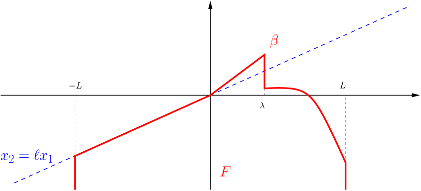
Figure 7.1. The barrier in Lemma 7.1.

Proof.

The geometric situation under consideration is depicted in Figure 7.1. Fixed $P=(P_{1},P_{2})\in\partial F$ with $P_{1}\in(0,\mu)$, as long as $\mu<\frac{\lambda}{2}$, we have that $P_{2}=\beta(P_{1})=(\bar{\ell}+\varepsilon a)\,P_{1}$, and we consider the tangent half-plane of $F$ through $P$. Namely, we define

$$\Pi_{P}:=\{(x_{1},x_{2})\in\mathbb{R}^{2}{\mbox{ s.t. }}x_{2}<(\bar{\ell}+\varepsilon a)(x_{1}-P_{1})+P_{2}\}.$$

Given $r>0$ and $R\in(r,+\infty]$, we also define

$$H_{P}(r,R):=\int_{B_{R}(P)\setminus B_{r}(P)}\frac{\big{(}\chi_{\mathbb{R}^{2}\setminus F}(y)-\chi_{F}(y)\big{)}-\big{(}\chi_{\mathbb{R}^{2}\setminus\Pi_{P}}(y)-\chi_{\Pi_{P}}(y)\big{)}}{|P-y|^{2+s}}\,dy,$$

with the obvious notation that the ball of radius $+\infty$ is simply the whole $\mathbb{R}^{2}$. Then, the desired claim is established once we prove that

$$H_{P}(0,+\infty)\leqslant 0.$$ (7.3)

The strategy for proving this is that the main positive contribution comes from the corner at the origin, and the rest of the barrier will provide negligible terms. To formalize this, we first observe that

$$\big{(}\chi_{\mathbb{R}^{2}\setminus F}(y)-\chi_{F}(y)\big{)}-\big{(}\chi_{\mathbb{R}^{2}\setminus\Pi_{P}}(y)-\chi_{\Pi_{P}}(y)\big{)}\leqslant 0\qquad{\mbox{for all }}y\in B_{\lambda/2}(P).$$ (7.4)

To check this, let $y\in B_{\lambda/2}(P)\cap\Pi_{P}$. Then, since $y\in\Pi_{P}$,

$$y_{2}<(\bar{\ell}+\varepsilon a)(y_{1}-P_{1})+P_{2}=(\bar{\ell}+\varepsilon a)(y_{1}-P_{1})+(\bar{\ell}+\varepsilon a)P_{1}=(\bar{\ell}+\varepsilon a)y_{1}.$$ (7.5)

Also, since $y\in B_{\lambda/2}(P)$, we have that

$$|y_{1}|\leqslant|y_{1}-P_{1}|+|P_{1}|\leqslant|y-P|+\mu<\frac{\lambda}{2}+\mu\leqslant\lambda,$$

and thus

$$\beta(y_{1})=\bar{\ell}y_{1}+\varepsilon ay_{1}\,\chi_{[0,\lambda]}(y_{1})\geqslant(\bar{\ell}+\varepsilon a)y_{1}.$$

This and (7.5) give that $y_{2}<\beta(y_{1})$, and thus $y\in F$. We have thereby established that $B_{\lambda/2}(P)\cap\Pi_{P}\subseteq F$, which proves (7.4).

Now, let

$${\mathcal{P}}:=\left\{(y_{1},y_{2})\in\mathbb{R}^{2}{\mbox{ s.t. }}y_{1}\in\left(-P_{1},-\frac{P_{1}}{2}\right){\mbox{ and }}y_{2}-\bar{\ell}y_{1}\in\left(-\frac{\varepsilon aP_{1}}{4},0\right)\right\}.$$ (7.6)

We observe that if $y\in{\mathcal{P}}$ we have that

$$\begin{split}&|y_{1}-P_{1}|\leqslant|y_{1}|+|P_{1}|<2P_{1}\\ {\mbox{ and }}&|y_{2}-P_{2}|\leqslant|y_{2}-\bar{\ell}y_{1}|+|\bar{\ell}|\,|y_{1}|+|P_{2}|<\frac{\varepsilon aP_{1}}{4}+|\bar{\ell}|\,P_{1}+|(\bar{\ell}+\varepsilon a)P_{1}|\\ &\qquad\qquad\leqslant\left(\frac{a}{4}+|\bar{\ell}|+(|\bar{\ell}|+a)\right)\,P_{1}\leqslant\left(\frac{a}{4}+\tilde{\ell}+(\tilde{\ell}+a)\right)\,P_{1}.\end{split}$$

Accordingly,

$${\mathcal{P}}\subseteq B_{C(\tilde{\ell},a)\,P_{1}}(P),$$ (7.7)

for some $C(\tilde{\ell},a)>0$.

We also claim that

$${\mathcal{P}}\subseteq F\setminus\Pi_{P}.$$ (7.8)

Indeed, if $y\in{\mathcal{P}}$, we know from (7.6) that $|y_{1}|<\lambda$, and thus $\beta(y_{1})=\bar{\ell}y_{1}+\varepsilon ay_{1}\,\chi_{[0,\lambda]}(y_{1})$. Consequently,

$$y_{2}-\beta(y_{1})=y_{2}-\bar{\ell}y_{1}-\varepsilon ay_{1}\,\chi_{[0,\lambda]}(y_{1})\leqslant y_{2}-\bar{\ell}y_{1}<0,$$

which says that $y\in F$. In addition,

$$y_{2}-(\bar{\ell}+\varepsilon a)(y_{1}-P_{1})-P_{2}=(y_{2}-\bar{\ell}y_{1})-\varepsilon ay_{1}>-\frac{\varepsilon aP_{1}}{4}+\frac{\varepsilon aP_{1}}{2}>0,$$

which says that $y\in\mathbb{R}^{2}\setminus\Pi_{P}$. These observations give (7.8).

Now, in light of (7.7) and (7.8), noticing that $C(\tilde{\ell},a)P_{1}\leqslant C(\tilde{\ell},a)\mu<\lambda/2$ as long as $\mu$ is sufficiently small (possibly in dependence of $\tilde{\ell}$ and $a$), we can write that

$${\mathcal{P}}\subseteq B_{\lambda/2}(P)\cap(F\setminus\Pi_{P}).$$ (7.9)

Also, since ${\mathcal{P}}$ is a parallelogram, its area $|{\mathcal{P}}|$ is equal to $\frac{\varepsilon aP_{1}^{2}}{8}$. From this, (7.4) and (7.9), and using again (7.7), we obtain that

$$-H_{P}(0,\lambda/2)\geqslant 2\int_{{\mathcal{P}}}\frac{dy}{|P-y|^{2+s}}\geqslant\frac{|{\mathcal{P}}|}{\big{(}C(\tilde{\ell},a)P_{1}\big{)}^{2+s}}=\frac{\varepsilon aP_{1}^{2}}{8\,\big{(}C(\tilde{\ell},a)P_{1}\big{)}^{2+s}}=\frac{C^{\prime}(\tilde{\ell},a)\,\varepsilon}{P_{1}^{s}},$$ (7.10)

for some $C^{\prime}(\tilde{\ell},a)>0$.

Now we take into account the contributions in $B_{L/2}(P)\setminus B_{\lambda/2}(P)$. To this end, let $y\in B_{L/2}(P)\setminus B_{\lambda/2}(P)$. If $y\in\Pi_{P}\setminus F$, we see that

$$\bar{\ell}y_{1}-\varepsilon a|y_{1}|-\varepsilon b|y_{1}|^{1+\alpha}\leqslant\beta(y_{1})\leqslant y_{2}\leqslant(\bar{\ell}+\varepsilon a)(y_{1}-P_{1})+P_{2}=(\bar{\ell}+\varepsilon a)y_{1}.$$

Consequently,

$$\begin{split}H_{P}(\lambda/2,L/2)\,&\leqslant 2\int_{\big{(}B_{L/2}(P)\setminus B_{\lambda/2}(P)\big{)}\cap(\Pi_{P}\setminus F)}\frac{dy}{|P-y|^{2+s}}\\ &\leqslant 2\int_{\big{(}B_{L/2}(P)\setminus B_{\lambda/2}(P)\big{)}\cap(\Pi_{P}\setminus F)}\frac{dy}{|P_{1}-y_{1}|^{2+s}}\\ &\leqslant 2\int_{\{|y_{1}|\in(\lambda/2,L/2)\}}\left[\int_{\bar{\ell}y_{1}-\varepsilon a|y_{1}|-\varepsilon b|y_{1}|^{1+\alpha}}^{(\bar{\ell}+\varepsilon a)y_{1}}\frac{dy_{2}}{|P_{1}-y_{1}|^{2+s}}\right]\,dy_{1}\\ &\leqslant 2\int_{\{|y_{1}|>\lambda/2\}}\frac{2\varepsilon a|y_{1}|+\varepsilon b|y_{1}|^{1+\alpha}}{|P_{1}-y_{1}|^{2+s}}\,dy_{1}\\ &\leqslant 2\int_{\{|t|>\lambda/4\}}\frac{2\varepsilon a(|t|+\lambda)+\varepsilon b(|t|+\lambda)^{1+\alpha}}{|t|^{2+s}}\,dt\\ &\leqslant C(s,a,b,\lambda,\alpha)\,\varepsilon,\end{split}$$ (7.11)

for some $C(s,a,b,\lambda,\alpha)>0$.

Finally, we see that

$$H_{P}(L/2,+\infty)\leqslant 2\int_{\mathbb{R}^{2}\setminus B_{L/2}(P)}\frac{dy}{|P-y|^{2+s}}=\frac{C_{0}}{L^{s}},$$

for some constant $C_{0}>0$.

Using this, (7.10) and (7.11), and recalling (7.1), we conclude that

$$H_{P}(0,+\infty) = H_{P}(0,\lambda/2)+H_{P}(\lambda/2,L/2)+H_{P}(L/2,+\infty)$$

$$\leqslant -\frac{C^{\prime}(\tilde{\ell},a)\,\varepsilon}{P_{1}^{s}}+C(s,a,b,\lambda,\alpha)\,\varepsilon+\frac{C_{0}}{L^{s}}$$

$$\leqslant \varepsilon\,\left(-\frac{C^{\prime}(\tilde{\ell},a)}{\mu^{s}}+C(s,a,b,\lambda,\alpha)+\frac{C_{0}}{c^{s}}\right)$$

$$\leqslant 0,$$

as long as

$$\mu<\left(\frac{C^{\prime}(\tilde{\ell},a)}{C(s,a,b,\lambda,\alpha)+\frac{C_{0}}{c^{s}}}\right)^{\frac{1}{s}},$$

and this completes the proof of (7.3), as desired. ∎

8. Boundary improvement of flatness for non-sticky points

A classical method to obtain regularity results is based on the iteration of a flatness principle, according to which graphs contained in a suitably narrow cylinder are necessarily contained in the interior in an even narrower cylinder, with estimates. In our situation, a result of this type cannot in general hold at the boundary, due to the stickiness phenomenon. Nevertheless, we will manage to produce a suitable version of an improvement of flatness scheme in all the cases that do not exhibit boundary discontinuities. The technical details of this scheme go as follows.

Theorem 8.1.

Let $\alpha\in(0,s)$, $\ell\in\mathbb{R}$, $u:\mathbb{R}\to\mathbb{R}$, with $u\in C^{1}([-h,0])$ for some $h>0$, and

$$E:=\{(x_{1},x_{2})\in\mathbb{R}^{2}{\mbox{ s.t. }}x_{2}<u(x_{1})\}.$$

Let $\varepsilon\in(0,1)$, and assume that $E$ is locally $s$-minimal in $(0,2^{\tilde{k}_{0}})\times\mathbb{R}$, where

$$\tilde{k}_{0}:=\left\lceil\frac{-\log\varepsilon}{c_{0}}\right\rceil.$$ (8.1)

Suppose also that

$$\lim_{x_{1}\searrow 0}u(x_{1})=0.$$ (8.2)

Then there exist $\tilde{\varepsilon}_{0}$, $c_{0}\in(0,1)$ such that if $\varepsilon\in(0,\tilde{\varepsilon}_{0}]$ the following statement holds true.

If

$$|u(x_{1})-\ell x_{1}|\leqslant\varepsilon^{\frac{1}{c_{0}}}\,|x_{1}|^{1+\alpha}{\mbox{ for all $x_{1}\in(-2^{\tilde{k}_{0}},0)$,}}$$ (8.3)

$$|u(x_{1})-\ell x_{1}|\leqslant\varepsilon(2^{k})^{1+\alpha}{\mbox{ for all $x_{1}\in(0,2^{k})$, for all $k\in\{0,\dots,\tilde{k}_{0}\}$,}}$$ (8.4)

then, for all $j\in\mathbb{N}$,

$$|u(x_{1})-\ell x_{1}|\leqslant\frac{\varepsilon}{(2^{j})^{1+\alpha}}\qquad{\mbox{ for all \;$x_{1}\in\left(0,\displaystyle\frac{1}{2^{j}}\right)$.}}$$ (8.5)

Moreover,

$$|u(x_{1})-\ell x_{1}|\leqslant 4\varepsilon\,x_{1}^{1+\alpha}\qquad{\mbox{ for all \;$x_{1}\in\left(0,\displaystyle\frac{1}{2}\right)$.}}$$ (8.6)

Proof.

We observe that (8.6) follows from (8.5), hence we focus on the proof of (8.5). Moreover, we can obtain (8.5) iteratively, that is, we prove it for $j=1$, then we scale and we apply it recursively.

Hence, the claims in Theorem 8.1 are established once we prove that

$$|u(x_{1})-\ell x_{1}|\leqslant\frac{\varepsilon}{2^{1+\alpha}}\qquad{\mbox{ for all \;$x_{1}\in\left(0,\displaystyle\frac{1}{2}\right)$.}}$$ (8.7)

To prove (8.7), we first exploit Lemma 6.2. In particular, by (6.12) and (6.13), fixed any $\delta\in(0,1)$, to be taken suitably small in what follows, we can write that

$$|u(x_{1})-\ell x_{1}-\varepsilon\bar{a}x_{1}^{\frac{1+s}{2}}|\leqslant C\varepsilon\,(x_{1}^{\frac{3+s}{2}}+\delta),$$ (8.8)

for all $x_{1}\in(0,3)$, for some $C>0$.

We claim that

$$\bar{a}=0.$$ (8.9)

To prove this, we argue by contradiction and we suppose that $\bar{a}>0$ (the case $\bar{a}<0$ can be treated similarly).

Without loss of generality, we can assume that $c_{0}\in(0,1)$ is so small that

$$\frac{\log 2}{c_{0}}\geqslant\frac{1}{s},$$ (8.10)

and $$1-\log 2-c_{0}>0.$$ (8.11)

We consider the barrier $\beta$ in Lemma 7.1, with $\bar{\ell}:=\ell+\varepsilon\delta$, $\lambda:=\min\left\{1,\frac{\bar{a}}{4C}\right\}$, $L:=\frac{1}{2\,\varepsilon^{\frac{\log 2}{c_{0}}}}$, $a:=\frac{\bar{a}}{8}$, $b:=2^{2+\alpha}+\frac{3}{\lambda^{1+\alpha}}$, $c:=\frac{1}{2}$. In this way, condition (7.1) is fulfilled, thanks to (8.10), and therefore Lemma 7.1 produces a suitable $\mu\in(0,1)$ such that (7.2) holds true (and, in our setting, we are taking $\varepsilon\ll\delta\ll\mu$). We slide the barrier of Lemma 7.1 from below till it touches $u$. To this end, we point out that the original barrier $\beta$ in Lemma 7.1 lies below $u$ in $(-\infty,0)\cup[\mu,+\infty)$.

Indeed, if $x_{1}\leqslant-L$ or $x_{1}\geqslant L$ the claim is obvious. If instead $x_{1}\in(-L,0)$, we observe that, by (8.1),

$$2^{\tilde{k}_{0}}\geqslant 2^{-1-\frac{\log\varepsilon}{c_{0}}}=\frac{1}{2\varepsilon^{\frac{\log 2}{c_{0}}}}=L.$$ (8.12)

Therefore, $x_{1}\in(-2^{\tilde{k}_{0}},0)$, and hence we use (8.3) and see that

$$\beta(x_{1})-u(x_{1})=\bar{\ell}x_{1}-u(x_{1})=\ell x_{1}-u(x_{1})-\varepsilon\delta|x_{1}|$$

$$\qquad\leqslant\varepsilon^{\frac{1}{c_{0}}}\,|x_{1}|^{1+\alpha}-\varepsilon\delta|x_{1}|\leqslant\varepsilon\,|x_{1}|(L^{\alpha}\varepsilon^{\frac{1-c_{0}}{c_{0}}}-\delta)$$

$$\qquad=\varepsilon\,|x_{1}|(\varepsilon^{\frac{1-c_{0}}{c_{0}}-\frac{\alpha\log 2}{c_{0}}}-\delta)<0,$$

as long as $\varepsilon$ is small enough (recall that $\frac{1-c_{0}}{c_{0}}-\frac{\alpha\log 2}{c_{0}}>0$, thanks to (8.11)).

If instead $x_{1}\in[\mu,\lambda]$, we exploit (8.8) and we write that

$$\beta(x_{1})-u(x_{1})=(\bar{\ell}+\varepsilon a)x_{1}-u(x_{1})=\left(\ell+\varepsilon\delta+\frac{\varepsilon\bar{a}}{8}\right)x_{1}-u(x_{1})$$

$$\qquad\leqslant\left(\varepsilon\delta+\frac{\varepsilon\bar{a}}{8}\right)x_{1}-\varepsilon\bar{a}x_{1}^{\frac{1+s}{2}}+C\varepsilon\,(x_{1}^{\frac{3+s}{2}}+\delta)$$

$$\qquad\leqslant\varepsilon\,x_{1}^{\frac{1+s}{2}}\,\left(\left(\delta+\frac{\bar{a}}{8}\right)x_{1}^{\frac{1-s}{2}}-\bar{a}+C\,\left(x_{1}+\frac{\delta}{x_{1}^{\frac{1+s}{2}}}\right)\right)$$

$$\qquad\leqslant\varepsilon\,x_{1}^{\frac{1+s}{2}}\,\left(2\left(\delta+\frac{\bar{a}}{8}\right)-\bar{a}+C\,\left(\frac{\bar{a}}{4C}+\frac{\delta}{\mu^{\frac{1+s}{2}}}\right)\right)$$

$$\qquad=\varepsilon\,x_{1}^{\frac{1+s}{2}}\,\left(-\frac{\bar{a}}{2}+2\delta+\frac{C\delta}{\mu^{\frac{1+s}{2}}}\right)<0.$$

Then, if $x_{1}\in[\lambda,1]$, we use (8.4) with $k:=0$ to write that $|u(x_{1})-\ell x_{1}|\leqslant\varepsilon$ and thus

$$\beta(x_{1})-u(x_{1})=(\ell+\varepsilon\delta)x_{1}-\varepsilon bx_{1}^{1+\alpha}-u(x_{1})\leqslant 2\varepsilon-\varepsilon b\lambda^{1+\alpha}<0.$$

Finally, if $x_{1}\in[1,L]$, recalling (8.12), we have that $x_{1}\in[1,2^{\tilde{k}_{0}}]$. Therefore, we can take $k\in\{0,\dots,\tilde{k}_{0}\}$ such that $2^{k-1}\leqslant x_{1}\leqslant 2^{k}$. Then, we recall (8.4) and we conclude that

$$|u(x_{1})-\ell x_{1}|\leqslant 2^{1+\alpha}\varepsilon x_{1}^{1+\alpha}.$$

Accordingly,

$$\beta(x_{1})-u(x_{1})=(\ell+\varepsilon\delta)x_{1}-\varepsilon bx_{1}^{1+\alpha}-u(x_{1})\leqslant 2^{1+\alpha}\varepsilon x_{1}^{1+\alpha}+\varepsilon\delta x_{1}-\varepsilon bx_{1}^{1+\alpha}$$

$$\qquad\leqslant\varepsilon x_{1}^{1+\alpha}\,\left(2^{1+\alpha}+\frac{\delta}{x_{1}^{\alpha}}-b\right)\leqslant\varepsilon x_{1}^{1+\alpha}\,\left(2^{1+\alpha}+1-b\right)<0.$$

With this, we can slide the barrier from below and deduce from (7.2) that $\beta\leqslant u$ in the whole $\mathbb{R}$.

Consequently, if we consider the second blow-up $E_{00}$ given in Lemma 2.2, we see that

$$\begin{split}E_{00}\;&\supseteq\{x=(x_{1},x_{2}){\mbox{ s.t. }}x_{1}>0{\mbox{ and }}x_{2}<(\bar{\ell}+\varepsilon a)x_{1}\}\\ &=\{x=(x_{1},x_{2}){\mbox{ s.t. }}x_{1}>0{\mbox{ and }}x_{2}<(\ell+\varepsilon(\delta+a))x_{1}\}.\end{split}$$ (8.13)

On the other hand, by (2.8) and (8.3),

$$E_{00}\cap\{x_{1}<0\}=\{x=(x_{1},x_{2}){\mbox{ s.t. }}x_{1}<0{\mbox{ and }}x_{2}<\ell x_{1}\}.$$

Using this, (8.13) and Theorem 4.1, we infer that

$$(0,\delta^{\prime})^{2}\subseteq E,$$ (8.14)

for some $\delta^{\prime}>0$. Indeed, Theorem 4.1 would give that either (8.14) is satisfied, or $(0,\delta^{\prime})^{2}\subseteq E^{c}$, but the latter possibility would give that $E_{00}\cap\{x_{1}>0\}=\varnothing$, which is in contradiction with (8.13).

As a consequence of (8.14), we have that

$$\lim_{x_{1}\searrow 0}u(x_{1})\geqslant\delta^{\prime},$$

which is in contradiction with (8.2) and thus it completes the proof of (8.9).

From this and (8.8), we conclude that

$${\mbox{for all }}x_{1}\in(0,2^{-k_{\star}}),\qquad|u(x_{1})-\ell x_{1}|\leqslant C\varepsilon\,(x_{1}^{\frac{3+s}{2}}+\delta)\leqslant\frac{\varepsilon}{2^{k_{\star}(1+\alpha)}},$$ (8.15)

for a sufficiently large $k_{\star}\in\mathbb{N}$, as long as $\delta>0$ is chosen small enough.

We remark that (8.15) is “almost” the desired result in (8.7), up to the “delay” produced by this $k_{\star}\in\mathbb{N}$ (which now plays the role of a universal constant). To remove such a delay, we take the freedom of further reducing the constant $c_{0}$ in (8.1), and we consider a rescaling by the factor $2^{1-k_{\star}}$, that is we consider the set $E_{\star}:=2^{1-k_{\star}}E$ and the function $u_{\star}(x_{1}):=2^{1-k_{\star}}u(2^{k_{\star}-1}x_{1})$.

In this way, we have that (8.3) and (8.4) are fulfilled with $\varepsilon$ replaced by $\varepsilon_{\star}:=2^{\alpha(k_{\star}-1)}\varepsilon$. To check this, we observe that, changing $\varepsilon$ to $\varepsilon_{\star}$ only affects the constant $c_{0}$ in (8.1), and therefore if $x_{1}\in(0,2^{k})$, then $2^{k_{\star}-1}x_{1}\in(0,2^{k+k_{\star}-1})$ and so, by (8.4),

$$|u_{\star}(x_{1})-\ell x_{1}|=2^{1-k_{\star}}|u(2^{k_{\star}-1}x_{1})-\ell(2^{k_{\star}-1}x_{1})|\leqslant 2^{1-k_{\star}}\varepsilon\,(2^{k+k_{\star}-1})^{1+\alpha}=\varepsilon_{\star}\,(2^{k})^{1+\alpha},$$

which is (8.4) with $u$ and $\varepsilon$ replaced by $u_{\star}$ and $\varepsilon_{\star}$, respectively.

Similarly, if $x_{1}\in(-2^{\tilde{k}_{0}},0)$, we write $2^{k_{\star}-1}x_{1}\in(-2^{\tilde{k}_{0}+k_{\star}-1},0)$ and exploit (8.3) to find that

$$|u_{\star}(x_{1})-\ell x_{1}|=2^{1-k_{\star}}|u(2^{k_{\star}-1}x_{1})-\ell(2^{k_{\star}-1}x_{1})|\leqslant 2^{1-k_{\star}}\,\varepsilon^{\frac{1}{c_{0}}}\,|2^{k_{\star}-1}x_{1}|^{1+\alpha}$$

$$\qquad\qquad=2^{\alpha(k_{\star}-1)}\,2^{\frac{\alpha(1-k_{\star})}{c_{0}}}\,\varepsilon_{\star}^{\frac{1}{c_{0}}}\,|x_{1}|^{1+\alpha}\leqslant\varepsilon_{\star}^{\frac{1}{c_{0}}}\,|x_{1}|^{1+\alpha}.$$

This says that (8.3) is satisfied with $u$ and $\varepsilon$ replaced by $u_{\star}$ and $\varepsilon_{\star}$, respectively.

Then, we are in the position of using (8.15) with $u$ and $\varepsilon$ replaced by $u_{\star}$ and $\varepsilon_{\star}$, and accordingly we see that

$$\sup_{y_{1}\in(0,1/2)}|u(y_{1})-\ell y_{1}|=2^{k_{\star}-1}\sup_{y_{1}\in(0,1/2)}|u_{\star}(2^{1-k_{\star}}y_{1})-\ell(2^{1-k_{\star}}y_{1})|$$

$$\qquad=2^{k_{\star}-1}\sup_{x_{1}\in(0,2^{-k_{\star}})}|u_{\star}(x_{1})-\ell x_{1}|\leqslant 2^{k_{\star}-1}\times\frac{\varepsilon_{\star}}{2^{k_{\star}(1+\alpha)}}=\frac{\varepsilon}{2^{1+\alpha}}.$$

This completes the proof of (8.7). ∎

From this, we obtain the following global regularity result:

Theorem 8.2.

Let $\alpha\in(0,s)$, $u:\mathbb{R}\to\mathbb{R}$, with

$$u\in C^{1,\alpha}([-h,0])$$ (8.16)

for some $h>0$, and

$$E:=\{(x_{1},x_{2})\in\mathbb{R}^{2}{\mbox{ s.t. }}x_{2}<u(x_{1})\}.$$

Assume that $E$ is locally $s$-minimal in $(0,1)\times\mathbb{R}$. Suppose also that

$$\lim_{x_{1}\searrow 0}u(x_{1})=\lim_{x_{1}\nearrow 0}u(x_{1}).$$ (8.17)

Then, $u\in C^{1,\alpha}(\left[-h,\frac{1}{2}\right])$.

Proof.

Up to a vertical translation, we can suppose that

the limit in (8.17) is equal to $0$, (8.18)

thus reducing to the setting in (8.2). Hence, the regularity in the interior is warranted by the results in [MR2675483], and the boundary regularity is a consequence of Theorem 8.1. Combining these two results, we obtain the desired $C^{1,\alpha}$-regularity up to the boundary. More precisely, one proves uniform pointwise $C^{1,\alpha}$-regularity at any given point by first exploiting the boundary improvement of flatness at the origin given by Theorem 8.1 up to a suitable scale, then switching the center of the improvement of flatness and applying there the interior improvement of flatness given by Theorem 6.8 of [MR2675483].

The technical details of the proof go as follows. First of all, we consider the double blow-up $E_{00}$ in Lemma 2.2. By (8.18) and Theorem 4.1, we obtain that

$$E_{00} E_{00}=\{x_{2}=\ell x_{1}\}$$ is a halfplane, say , (8.19)

for some $\ell\in\mathbb{R}$. As a matter of fact, by (8.16), we have that $\ell=u^{\prime}(0^{-})$.

Now we define $\varepsilon_{\star}$ to be the minimum between the $\tilde{\varepsilon}_{0}$ in Theorem 8.1 here and the corresponding quantity in Theorem 6.8 of [MR2675483]. Similarly, we take $\tilde{k}_{0}$ as in Theorem 8.1 (with $\varepsilon$ there taken to be equal to $\tilde{\varepsilon}_{0}$). Then, we take $\tilde{k}_{\star}$ to be the maximum between such a $\tilde{k}_{0}$ and the corresponding quantity in Theorem 6.8 of [MR2675483]. From now on, $\varepsilon_{\star}$ and $\tilde{k}_{\star}$ will be fixed quantities. Then, we use (8.19) and Corollary C.2, to find $k_{\star}$, only depending on the fixed $\varepsilon_{\star}$ and $\tilde{k}_{\star}$, such that $\partial E_{k_{\star}}$ lies locally so close to $\partial E_{00}$ that

$$|u_{\star}(x_{1})-\ell x_{1}|\leqslant\frac{\varepsilon_{\star}}{2^{\tilde{k}_{\star}(1+\alpha)+10}}\qquad{\mbox{ for all }}x_{1}\in(-2^{\tilde{k}_{\star}+1},2^{\tilde{k}_{\star}+1}),$$ (8.20)

where

$$u_{\star}(x_{1}):=k_{\star}u\left(\frac{x_{1}}{k_{\star}}\right).$$ (8.21)

For further use, we remark that, in view of (8.20), for all $k\in\{0,\dots,\tilde{k}_{\star}\}$,

$$|u_{\star}(x_{1})-\ell x_{1}|\leqslant\frac{\varepsilon_{\star}}{{2^{\tilde{k}_{\star}(1+\alpha)+10}}}\leqslant\frac{\varepsilon_{\star}}{{2^{\tilde{k}_{\star}(1+\alpha)+10}}}(2^{k})^{1+\alpha}\qquad{\mbox{ for all }}x_{1}\in(0,2^{k}).$$ (8.22)

Then, Theorem 8.2 is proven once we show that, for all $\bar{x}_{1}$, $\bar{y}_{1}\in\left[0,\frac{1}{2}\right]$, there exists $\ell_{\bar{y}_{1}}\in\mathbb{R}$ such that

$$|u_{\star}(\bar{x}_{1})-u_{\star}(\bar{y}_{1})-\ell_{\bar{y}_{1}}(\bar{x}_{1}-\bar{y}_{1})|\leqslant C\,|\bar{x}_{1}-\bar{y}_{1}|^{1+\alpha},$$ (8.23)

for a suitable $C>0$, since a similar estimate for $u$, up to changing $C$, would follow directly from (8.23) and (8.21).

To prove this, we let $d:=\frac{|\bar{x}_{1}-\bar{y}_{1}|}{2}$ and $z:=\frac{\bar{x}_{1}+\bar{y}_{1}}{2}$. We distinguish two cases: either $z\in[0,2d]$, or $z\in\left(2d,\frac{1}{2}\right]$. To start with, let us suppose that $z\in[0,2d]$. In this case, we deduce from (8.22) that

$$|u_{\star}(x_{1})-\ell x_{1}|\leqslant\tilde{\varepsilon}_{0}(2^{k})^{1+\alpha}\qquad{\mbox{ for all }}x_{1}\in(0,2^{k}).$$

Consequently, the assumption in (8.4) is satisfied by $u_{\star}$. Furthermore, using (8.16), we have that, if $x_{1}\in(-h,0)$,

$$|u(x_{1})-\ell x_{1}|=|u(x_{1})-u(0)-u^{\prime}(0^{-})x|\leqslant C|x_{1}|^{1+\alpha},$$

for some $C>0$, and accordingly, if $x_{1}\in(-hk_{\star},0)$

$$|u_{\star}(x_{1})-\ell x_{1}|\leqslant\frac{C}{k_{\star}^{\alpha}}\,|x_{1}|^{1+\alpha}.$$

This says that, possibly enlarging $k_{\star}$ by a fixed amount, also the condition in (8.3) is satisfied by $u_{\star}$.

Hence, we are in the position of using Theorem 8.1 on $u_{\star}$, thus deducing from (8.6) that, for all $x_{1}\in\left(0,\displaystyle\frac{1}{2}\right)$,

$$|u_{\star}(x_{1})-\ell x_{1}|\leqslant 4\tilde{\varepsilon}_{0}\,x_{1}^{1+\alpha}.$$

As a consequence,

$$|u_{\star}(\bar{x}_{1})-u_{\star}(\bar{y}_{1})-\ell(\bar{x}_{1}-\bar{y}_{1})|\leqslant|u_{\star}(\bar{x}_{1})-\ell\bar{x}_{1}|+|u_{\star}(\bar{y}_{1})-\ell\bar{y}_{1}|\leqslant 4\tilde{\varepsilon}_{0}\,\big{(}\bar{x}_{1}^{1+\alpha}+\bar{y}_{1}^{1+\alpha}\big{)}.$$

Hence, since

$$\frac{\bar{x}_{1}}{2},\,\frac{\bar{y}_{1}}{2}\leqslant\frac{\bar{x}_{1}+\bar{y}_{1}}{2}=z\leqslant 2d=|\bar{x}_{1}-\bar{y}_{1}|,$$

we conclude that

$$|u_{\star}(\bar{x}_{1})-u_{\star}(\bar{y}_{1})-\ell(\bar{x}_{1}-\bar{y}_{1})|\leqslant 32\tilde{\varepsilon}_{0}\,|\bar{x}_{1}-\bar{y}_{1}|^{1+\alpha},$$

and this establishes (8.23) with $\ell_{\bar{y}_{1}}:=\ell$ when $z\in[0,2d]$.

Hence, we suppose now that

$$z\in\left(2d,\frac{1}{2}\right]$$ (8.24)

and we prove (8.23) also in this case. To this end, we set

$$\tilde{u}(x_{1}):=\frac{u_{\star}(z(1+x_{1}))}{z}.$$ (8.25)

Then, $\tilde{u}$ describes a nonlocal minimal graph in $\left(-1,\frac{1}{z}-1\right)$, which contains $(-1,1)$. Moreover,

$$\begin{split}&|\tilde{u}(x_{1})-\tilde{u}(0)-\ell x_{1}|=\frac{1}{z}\,\big{|}u_{\star}(z(1+x_{1}))-z\ell x_{1}-u_{\star}(z)\big{|}\\ &\qquad\leqslant\frac{1}{z}\,\Big{(}\big{|}u_{\star}(z(1+x_{1}))-\ell(z(1+x_{1}))\big{|}+|u_{\star}(z)-\ell z|\Big{)}.\end{split}$$ (8.26)

On the other hand, by (8.22), and recalling also (8.6), for all $x_{1}\in(0,2^{\tilde{k}_{\star}})$,

$$|u_{\star}(x_{1})-\ell x_{1}|\leqslant\frac{\varepsilon_{\star}}{{2^{\tilde{k}_{\star}(1+\alpha)+8}}}\,x_{1}^{1+\alpha}.$$

Hence, for all $x_{1}\in(-1,1)$,

$$\big{|}u_{\star}(z(1+x_{1}))-\ell(z(1+x_{1}))\big{|}\leqslant\frac{\varepsilon_{\star}}{{2^{\tilde{k}_{\star}(1+\alpha)+6}}}\,z^{1+\alpha}(1+x_{1})^{1+\alpha}\leqslant\frac{\varepsilon_{\star}}{{2^{\tilde{k}_{\star}(1+\alpha)+4}}}z^{1+\alpha}.$$

This and (8.26) give that, if $k\in\{0,\dots,\tilde{k}_{\star}\}$ and $x_{1}\in(-2^{-k},2^{-k})$,

$$|\tilde{u}(x_{1})-\tilde{u}(0)-\ell x_{1}|\leqslant\frac{\varepsilon_{\star}\,z^{\alpha}}{2^{\tilde{k}_{\star}(1+\alpha)}}\leqslant\frac{\varepsilon_{\star}\,z^{\alpha}}{2^{k(1+\alpha)}}.$$

Hence, by Theorem 6.8 of [MR2675483], for all $x_{1}$, $y_{1}\in\left(-\frac{1}{2},\frac{1}{2}\right)$,

$$|\tilde{u}(x_{1})-\tilde{u}(y_{1})-\tilde{u}^{\prime}(y_{1})(x_{1}-y_{1})|\leqslant C\varepsilon_{\star}\,z^{\alpha}\,|x_{1}-y_{1}|^{1+\alpha},$$ (8.27)

for some $C>0$.

Now, we suppose that $\bar{x}_{1}\leqslant\bar{y}_{1}$ (the case $\bar{x}_{1}>\bar{y}_{1}$ can be treated in a similar way). Then, we have that $\bar{x}_{1}=z-d$ and $\bar{y}_{1}=z+d$. Hence, since $\frac{d}{z}<\frac{1}{2}$ thanks to (8.24), we are in the position of utilizing (8.25) and (8.27) (taking $\ell_{\bar{y}_{1}}:=\tilde{u}^{\prime}(y_{1})$, with $x_{1}:=-\frac{d}{z}$ and $y_{1}:=\frac{d}{z}$) and conclude that

$$|u_{\star}(\bar{x}_{1})-u_{\star}(\bar{y}_{1})-\ell_{\bar{y}_{1}}(\bar{x}_{1}-\bar{y}_{1})|=|u_{\star}(z-d)-u_{\star}(z+d)+2\ell_{\bar{y}_{1}}d|$$

$$\qquad=\left|z\tilde{u}\left(-\frac{d}{z}\right)-z\tilde{u}\left(\frac{d}{z}\right)+2\ell_{\bar{y}_{1}}d\right|\leqslant C\varepsilon_{\star}\,z^{1+\alpha}\,\left(\frac{2d}{z}\right)^{1+\alpha}\leqslant 4C\varepsilon_{\star}\,d^{1+\alpha}.$$

Up to renaming $C$, this completes the proof of (8.23), as desired. ∎

9. Boundary regularity, and proof of Theorem 1.2

While Theorem 8.2 has its own interest, since it says that nonlocal minimal graphs which are not boundary discontinuous are necessarily $C^{1,\alpha}$ up to the boundary, for concrete applications of such a result it is essential to improve the value of $\alpha$ (provided that the exterior datum is regular enough): in particular, the Hölder exponent needed to pass the equation to the limit at boundary points needs to be higher than $s$, while the one coming from Theorem 8.2 happens to be less than $s$. From the technical point of view, this is due to the possible growth of the solution at infinity and the long range interactions of the problem.

Our objective is now to modify and extend some linearization methods in [MR3331523], combined with some precise boundary asymptotics of fractional Laplace equations, taking into account the additional boundary effects, to improve the Hölder exponent in Theorem 8.2 and finally obtain Theorem 1.2.

Proof of Theorem 1.2.

We take $\zeta\in C^{\infty}_{0}\left(\left[-\frac{h}{2},\frac{h}{2}\right],\,[0,1]\right)$ with $\zeta=1$ in $\left(-\frac{h}{4},\frac{h}{4}\right)$, and we define

$$v(x_{1}):=\zeta(x_{1})\,u(x_{1}).$$

Using formula (49) in [MR3331523], and recalling the notation in (6.8), we have that, for all $x_{1}\in(0,1)$,

$$\int_{\mathbb{R}}F\left(\frac{u(x_{1}+t)-u(x_{1})}{|t|}\right)\,\frac{dt}{|t|^{1+s}}=0,$$ (9.1)

in the principal value sense.

We also recall that $u^{\prime}(x_{1})$ is well defined, thanks to the interior regularity in [MR3090533], and therefore, by odd symmetry, and using that $F$ is bounded, for any $J\subseteq\mathbb{R}$ which is symmetric with respect to the origin, we obtain that

$$\begin{split}&\int_{J}F\left(\frac{u(x_{1}+t)-u(x_{1})}{|t|}\right)\,\frac{dt}{|t|^{1+s}}\\ =\;&\int_{J}\left[F\left(\frac{u(x_{1}+t)-u(x_{1})}{|t|}\right)-F\left(\frac{u^{\prime}(x_{1})\,t}{|t|}\right)\right]\,\frac{dt}{|t|^{1+s}}\\ =\;&\int_{J}\Big{(}u(x_{1}+t)-u(x_{1})-u^{\prime}(x_{1})\,t\Big{)}\,\frac{a(x_{1},t)\,dt}{|t|^{2+s}}\\ =\;&\int_{J}\delta(x_{1},t)\,\frac{a(x_{1},t)\,dt}{|t|^{2+s}},\end{split}$$ (9.2)

where

$$a(x_{1},t):=\int_{0}^{1}F^{\prime}\left(\frac{\tau\big{(}u(x_{1}+t)-u(x_{1})\big{)}+(1-\tau)u^{\prime}(x_{1})\,t}{|t|}\right)\,d\tau$$

and $$\delta(x_{1},t):=u(x_{1}+t)-u(x_{1})-u^{\prime}(x_{1})\,t.$$

In particular, choosing $J:=\mathbb{R}$, we deduce from (9.1) and (9.2) that

$$\int_{\mathbb{R}}\delta(x_{1},t)\,\frac{a(x_{1},t)\,dt}{|t|^{2+s}}=0.$$

As a consequence, if $\sigma:=\frac{1+s}{2}$, $I:=\left(-\frac{h}{4},\frac{h}{4}\right)$, and $x_{1}\in\left(0,\frac{h}{4}\right)$,

$$\begin{split}&-F^{\prime}\big{(}u^{\prime}(x_{1})\big{)}\,(-\Delta)^{\sigma}v(x_{1})\\ =\;&F^{\prime}\big{(}u^{\prime}(x_{1})\big{)}\,\int_{\mathbb{R}}\Big{(}v(x_{1}+t)-v(x_{1})-v^{\prime}(x_{1})\,t\Big{)}\,\frac{dt}{|t|^{2+s}}\\ =\;&F^{\prime}\big{(}u^{\prime}(x_{1})\big{)}\,\int_{I}\Big{(}u(x_{1}+t)-u(x_{1})-u^{\prime}(x_{1})\,t\Big{)}\,\frac{dt}{|t|^{2+s}}\\ &\qquad\qquad+F^{\prime}\big{(}u^{\prime}(x_{1})\big{)}\,\int_{\mathbb{R}\setminus I}\Big{(}v(x_{1}+t)-u(x_{1})-u^{\prime}(x_{1})\,t\Big{)}\,\frac{dt}{|t|^{2+s}}\\ =\;&\int_{I}\delta(x_{1},t)\,\frac{a(x_{1},t)\,dt}{|t|^{2+s}}\,dt+\int_{I}\delta(x_{1},t)\,\frac{F^{\prime}\big{(}u^{\prime}(x_{1})\big{)}-a(x_{1},t)}{|t|^{2+s}}\,dt\\ &\qquad\qquad+F^{\prime}\big{(}u^{\prime}(x_{1})\big{)}\,\int_{\mathbb{R}\setminus I}\Big{(}v(x_{1}+t)-u(x_{1})-u^{\prime}(x_{1})\,t\Big{)}\,\frac{dt}{|t|^{2+s}}\\ =\;&f(x_{1}),\end{split}$$ (9.3)

where

$$\begin{split}&f_{1}(x_{1}):=-\int_{\mathbb{R}\setminus I}\delta(x_{1},t)\,\frac{a(x_{1},t)\,dt}{|t|^{2+s}},\\ &f_{2}(x_{1}):=\int_{I}\delta(x_{1},t)\,\frac{F^{\prime}\big{(}u^{\prime}(x_{1})\big{)}-a(x_{1},t)}{|t|^{2+s}}\,dt\\ &f_{3}(x_{1}):=F^{\prime}\big{(}u^{\prime}(x_{1})\big{)}\,\int_{\mathbb{R}\setminus I}\Big{(}v(x_{1}+t)-u(x_{1})-u^{\prime}(x_{1})\,t\Big{)}\,\frac{dt}{|t|^{2+s}},\\ {\mbox{and }}\;&f(x_{1}):=f_{1}(x_{1})+f_{2}(x_{1})+f_{3}(x_{1}).\end{split}$$ (9.4)

Now we use the following notation: given $r\in\mathbb{R}$ we denote by $\underline{r}$ a real number strictly smaller than $r$ which can be taken as close as we want to $r$. For instance, the thesis in Theorem 8.2 can be written as $u\in C^{1,\underline{s}}([0,1/2])$, with continuity of the derivative of $u$ at the origin with respect to the external datum. We claim that if $u\in L^{\infty}\left([0,h]\right)\cap C^{1,{\tilde{\alpha}}}\left(\left[0,\frac{h}{2}\right]\right)$ for some

$${\tilde{\alpha}}\in\left(\frac{s}{2},1\right)\setminus\{s\},$$ (9.5)

then

$$\begin{split}&f\in C^{\kappa({\tilde{\alpha}})}\left(\left[0,\frac{h}{4}\right]\right),{\mbox{ with }}\|f\|_{C^{\kappa({\tilde{\alpha}})}\left(\left[0,\frac{h}{4}\right]\right)}\leqslant C_{{\tilde{\alpha}},s},\\ {\mbox{where }}\;&\kappa({\tilde{\alpha}}):=\min\{{{\tilde{\alpha}}},2{\tilde{\alpha}}-s\},\end{split}$$ (9.6)

for some $C_{{\tilde{\alpha}},s}>0$ depending only on $s$, ${\tilde{\alpha}}$, $h$, and $\|u\|_{C^{1,{\tilde{\alpha}}}\left(\left[0,\frac{h}{2}\right]\right)}$.

The proof of (9.6) is rather complicated and it is based on a long and delicate computation. Not to interrupt the flow of ideas, we postpone this proof to Appendix D.

We now define

$$f_{\star}(x_{1}):=-\frac{f(x_{1})}{F^{\prime}(u(x_{1}))},$$

and we deduce from (9.6) that

$$f_{\star}\in C^{\kappa({\tilde{\alpha}})}\left(\left[0,\frac{h}{4}\right]\right).$$ (9.7)

Now we recall that $v$ belongs to $C^{1,{{\alpha}}}\left([-h,0]\right)$, and also to $C^{\infty}\left(\left(\frac{h}{4},2h\right)\right)$, thanks to the regularity of $u$ established in [MR3090533, MR3331523]. Therefore, we can take a function

$$\tilde{v}\in C^{1,{{\alpha}}}\left(\left[-\frac{h}{2},\frac{h}{2}\right]\right)$$ (9.8)

such that $\tilde{v}=v$ outside $\left(0,\frac{h}{4}\right)$.

We observe that, by construction, $\tilde{v}(0)=v(0)=u(0)=0$ and $\tilde{v}^{\prime}(0)=v^{\prime}(0)=u^{\prime}(0)$. Hence, as $|x_{1}|\to 0$,

$$\tilde{v}(x_{1})=u^{\prime}(0)x_{1}+O(|x_{1}|^{1+{{\alpha}}}).$$ (9.9)

Furthermore, by (9.8), see e.g. Proposition 2.1.8 in [MR2707618], we have that $g_{\star}:=(-\Delta)^{\sigma}\tilde{v}\in C^{1+{{\alpha}}-2\sigma}\left(\left[0,\frac{h}{4}\right]\right)$. Hence, setting $h_{\star}:=f_{\star}-g_{\star}$, we deduce from (9.7) that

$$h_{\star}\in C^{\vartheta}\left(\left[0,\frac{h}{4}\right]\right),\qquad{\mbox{ with }}\vartheta:=\min\{\sigma,\,\kappa({\tilde{\alpha}}),\,1+{{\alpha}}-2\sigma\}.$$ (9.10)

Notice that $\vartheta\in(0,1)$, since ${{\alpha}}>s$.

Let also $W:=v-\tilde{v}$ and $\tilde{W}(x_{1}):=x_{1}^{-\sigma}W(x_{1})$. By (9.3), we see that

$$\begin{cases}(-\Delta)^{\sigma}W=h_{\star}&{\mbox{ in }}\left(0,\displaystyle\frac{h}{4}\right),\\ W=0&{\mbox{ in }}\mathbb{R}\setminus\left(0,\displaystyle\frac{h}{4}\right).\end{cases}$$

Hence, using (9.10) and Lemma B.2, we deduce that

$$v(x_{1})-\tilde{v}(x_{1})=W(x_{1})=x_{1}^{\sigma}\tilde{W}(x_{1})=x_{1}^{\sigma}\Big{(}a_{0}+O\big{(}x_{1}^{\mu}\big{)}\Big{)}$$ (9.11)

as $x_{1}\searrow 0$, for a suitable $a_{0}\in\mathbb{R}$, with

$$\mu:=\min\{1,\,{\underline{\vartheta}+\sigma}\}=\min\{1,\,\underline{2\sigma},\,\kappa({\tilde{\alpha}})+\underline{\sigma},\,1+\underline{{{\alpha}}}-\sigma\}.$$

On the other hand, by (9.9) and Theorem 8.2, we know that

$$v(x_{1})-\tilde{v}(x_{1})=u(x_{1})-u^{\prime}(0)x_{1}+O(x_{1}^{1+{{\alpha}}})=O(x_{1}^{1+{\tilde{\alpha}}}),$$ (9.12)

as $x_{1}\searrow 0$. Combining this and (9.11), we conclude that

$$a_{0}=\lim_{x_{1}\searrow 0}a_{0}+O\big{(}x_{1}^{\mu}\big{)}=\lim_{x_{1}\searrow 0}x_{1}^{-\sigma}\Big{(}v(x_{1})-\tilde{v}(x_{1})\Big{)}=\lim_{x_{1}\searrow 0}O(x_{1}^{1+{\tilde{\alpha}}-\sigma})=0.$$

Therefore, we can write (9.11) as $W(x_{1})=O\big{(}x_{1}^{\mu+\sigma}\big{)}$, and then exploit Lemma B.3 to deduce that $W\in C^{\mu+\sigma}\left(\left[0,\frac{h}{8}\right]\right)$. As a consequence, recalling (9.8), we find that $v=W+\tilde{v}\in C^{\xi({\tilde{\alpha}})}\left(\left[0,\frac{h}{8}\right]\right)$, with

$$\xi({\tilde{\alpha}}):=\min\{\mu+\sigma,\,1+{{\alpha}}\}=\min\left\{\frac{3+s}{2},\,1+\underline{{{\alpha}}},\,\kappa({\tilde{\alpha}})+1+\underline{s}\right\}\in(1+s,2).$$

This gives that

$$u\in C^{1,\xi({\tilde{\alpha}})-1}\left(\left[0,\frac{h}{2}\right]\right).$$ (9.13)

We can now bootstrap this procedure till we reach an almost optimal Hölder exponent for $u^{\prime}$. Namely, in view of Theorem 8.2, we know that $u\in C^{1,\alpha_{1}}\left(\left[0,\frac{h}{2}\right]\right)$, with $\alpha_{1}:=\underline{s}$. Then, by (9.13), we obtain that $u\in C^{1,\alpha_{2}}\left(\left[0,\frac{h}{2}\right]\right)$, with $\alpha_{2}:=\min\left\{\frac{1+s}{2},\,{{\alpha}},\,\kappa(\alpha_{1})+s\right\}$.

Iterating this, for all $k\in\mathbb{N}$ with $k\geqslant 2$, we conclude that

$$u\in C^{1,\alpha_{k}}\left(\left[0,\frac{h}{2}\right]\right),\qquad{\mbox{ with }}\qquad\alpha_{k}:=\min\left\{\frac{1+s}{2},\,{{\alpha}},\,\kappa(\alpha_{k-1})+s\right\}.$$ (9.14)

We claim that there exists $k\in\mathbb{N}$, $k\leqslant 4+\frac{1}{s}$, such that

$$\kappa(\alpha_{k-1})+s\geqslant\min\left\{\frac{1+s}{2},\,{{\alpha}}\right\}.$$ (9.15)

Indeed, if not, we have that

$$\kappa(\alpha_{k-1})+s<\min\left\{\frac{1+s}{2},\,{{\alpha}}\right\},$$ (9.16)

for all $k\leqslant 4+\frac{1}{s}$. Accordingly, we obtain that $\alpha_{k}=\kappa(\alpha_{k-1})+s$, for all $k\leqslant 4+\frac{1}{s}$. In addition, by (9.14), we have that $\alpha_{k}>s$ for all $k\geqslant 2$, and therefore, by (9.6), if $k\geqslant 3$,

$$\kappa(\alpha_{k-1})=\min\{{\alpha_{k-1}},2\alpha_{k-1}-s\}={\alpha_{k-1}}.$$

Hence, for all $k\in\mathbb{N}\cap[3,4+\frac{1}{s}]$, and all $j\in\mathbb{N}$, with $j\leqslant k-2$,

$$\alpha_{k}={\alpha_{k-1}}+s\geqslant\alpha_{k-1}+\frac{s}{2}\geqslant\dots\geqslant\alpha_{k-j}+\frac{sj}{2}.$$

In particular, taking $k\in\left(3+\frac{1}{s},4+\frac{1}{s}\right]$

$$\alpha_{k}\geqslant\alpha_{2}+\frac{s(k-2)}{2}\geqslant\frac{s(k-2)}{2}\geqslant\frac{1+s}{2},$$

which is in contradiction with (9.16), and so it proves (9.15).

Hence, by (9.14) and (9.15),

$$u\in C^{1,\gamma}\left(\left[0,\frac{h}{2}\right]\right),\qquad{\mbox{ with }}\qquad\gamma:=\min\left\{\frac{1+s}{2},\,{{\alpha}}\right\}.$$

This completes the proof of Theorem 1.2. ∎

10. Boundary validity of the nonlocal curvature equation, and proof of Theorem 1.4

With the previous work, we are now ready to obtain that the Euler-Lagrange equation is satisfied pointwise at all points which are accessible from the interior (being evidently false elsewhere).

Proof of Theorem 1.4.

For interior points, that is when $x\in(\partial E)\cap((0,1)\times\mathbb{R})$, in view of [MR2675483], we know that (1.7) is satisfied in the viscosity sense. But since in this case $(\partial E)\cap((0,1)\times\mathbb{R})$ is locally a $C^{\infty}$ set, thanks to [MR3090533, MR3331523], we conclude that (1.7) is also satisfied in the pointwise sense at every point of $x\in(\partial E)\cap((0,1)\times\mathbb{R})$.

Hence, to complete the proof of Theorem 1.4, we only have to take into account the boundary points, i.e., the points which lie on the boundary of the slab and can be reached by points lying in $(\partial E)\cap((0,1)\times\mathbb{R})$.

For this, we distinguish two cases. If $u$ is discontinuous at the boundary point, the result follows by suitably applying the results in [MR3532394], see e.g. Theorem B.9 in [CLAUDIALUCA] for a detailed statement.

If instead $u$ is continuous at the boundary point, we first write (1.7) at interior points. That is, using the notation in (6.8) and recalling formula (49) in [MR3331523], we have that

$$\begin{split}&\int_{\mathbb{R}}\left[F\left(\frac{u(x_{1}+w)-u(x_{1})}{|w|}\right)-F\left(\frac{u^{\prime}(x_{1})\,w}{|w|}\right)\right]\,\frac{dw}{|w|^{1+s}}\\ &\qquad=\int_{\mathbb{R}}F\left(\frac{u(x_{1}+w)-u(x_{1})}{|w|}\right)\,\frac{dw}{|w|^{1+s}}=0,\end{split}$$ (10.1)

for all $x_{1}\in(0,1)$.

We also observe that, for small $x_{1}>0$,

$$\begin{split}&\left[F\left(\frac{u(x_{1}+w)-u(x_{1})}{|w|}\right)-F\left(\frac{u^{\prime}(x_{1})\,w}{|w|}\right)\right]\,\frac{1}{|w|^{1+s}}\\ &\qquad\qquad\leqslant C\,\min\left\{\frac{1}{|w|^{1+s}},\,\frac{1}{|w|^{1+s-\min\left\{{{\alpha}},\frac{1+s}{2}\right\}}}\right\},\end{split}$$ (10.2)

for some $C>0$, thanks to Theorem 1.2, and the function on the right hand side of (10.2) belongs to $L^{1}(\mathbb{R})$.

As a consequence, we obtain the desired claim in (1.7) taking the limit in (10.1), by the Dominated Convergence Theorem. ∎

11. Genericity of the stickiness phenomenon, and proof of Theorem 1.1

Now we are ready to prove our main result concerning the genericity of boundary discontinuities for nonlocal minimal graphs in the plane.

Proof of Theorem 1.1.

First of all, we observe that, for all $t\geqslant 0$ and $x_{1}\in\mathbb{R}$,

$$u(x_{1},t)\geqslant u(x_{1},0).$$ (11.1)

To prove this, we recall Lemma 3.3 in [MR3516886], according to which

$$(0,1)\times(-\infty,-M_{t})\subseteq E_{t}\cap\Omega\subseteq(0,1)\times(-\infty,M_{t}),$$

for some $M_{t}>0$. As a consequence, if $\tau>M_{t}+M_{0}$, we have that

$$E_{t}+\tau e_{2}\supset E_{0},$$

where, as customary, we set $e_{2}:=(0,1)$.

Thus, we reduce $\tau$ till the first contact between the two sets. Since $\varphi$ is nonnegative and supported away from $(-d,1+d)$, we have that this contact $\tau$ is necessarily nonnegative. We show that $\tau=0$, which in turn proves (11.1). Indeed, if $\tau>0$, the touching point $p$ between $E_{t}+\tau e_{2}$ and $E_{0}$ must necessarily occur in $\overline{\Omega}$. As a consequence

$$0=H^{s}_{E_{t}+\tau e_{2}}(p)=\int_{\mathbb{R}^{2}}\frac{\chi_{\mathbb{R}^{2}\setminus(E_{t}+\tau e_{2})}(y)-\chi_{E_{t}+\tau e_{2}}(y)}{|p-y|^{2+s}}\,dy$$

$$\qquad\leqslant\int_{\mathbb{R}^{2}}\frac{\chi_{\mathbb{R}^{2}\setminus E_{0}}(y)-\chi_{E_{0}}(y)}{|p-y|^{2+s}}\,dy=H^{s}_{E_{0}}(p)=0.$$

In particular, this says that $E_{t}+\tau e_{2}$ and $E_{0}$ must coincide, which is impossible since $\varphi$ does not vanish identically. This proves (11.1).

Now, we focus on the proof of (1.5). To prove (1.5), we assume the converse inequality and we show that $\varphi$ vanishes identically, which is against our assumption.

More precisely, if (1.5) were not true, then there would be $T>0$ such that for all $t\in[0,T]$

$$\limsup_{{x_{1}\searrow 0}}u(x_{1},t)\leqslant v(0).$$

Hence, by (1.4) and (11.1),

$$\limsup_{{x_{1}\searrow 0}}u(x_{1},t)=v(0).$$

Then, by Theorem 1.4, we would find that

$$\int_{\mathbb{R}}F\left(\frac{u(w,t)-v(0)}{|w|}\right)\,\frac{dw}{|w|^{1+s}}=0,$$

for all $t\in[0,T]$, and therefore

$$\int_{\mathbb{R}}\left[F\left(\frac{u(w,t)-v(0)}{|w|}\right)-F\left(\frac{u(w,0)-v(0)}{|w|}\right)\right]\,\frac{dw}{|w|^{1+s}}=0.$$ (11.2)

On the other hand, recalling (6.8), we notice that $F$ is strictly increasing. Consequently, by (11.1), we would find that

$$F\left(\frac{u(w,t)-v(0)}{|w|}\right)-F\left(\frac{u(w,0)-v(0)}{|w|}\right)\geqslant 0,$$ (11.3)

with strict inequality unless

$$u(w,t)=u(w,0) w\in\mathbb{R}$$ for all . (11.4)

In particular, since the strict inequality in (11.3) is excluded by (11.2), we obtain that (11.4) is necessarily satisfied, for all $t\in[0,T]$.

Taking $w$ outside $(0,1)$, we would thus conclude that

$$v(w)+t\varphi(w)=u(w,t)=u(w,0)=v(w),$$

for all $t\in[0,T]$, which would give that $\varphi$ vanishes identically, against our assumption. ∎

Appendix A Blow-up methods and proofs of the technical statements in Section 2

This appendix contains the proofs of the auxiliary results stated in Section 2. The details of this proofs are not easily accessible in the literature, since they deal with the newly explored setting of boundary blow-up methods for nonlocal minimal surfaces, but we postponed these technical arguments not to interrupt the main line of reasoning.

Proof of Lemma 2.1.

We observe that $E\setminus\Omega$ is a Lipschitz set in $B_{r_{0}}$, therefore, for all $r\in(0,r_{0})$,

$$\begin{split}&\iint_{(\Omega\cap B_{r})\times(\Omega^{c}\cap B_{r})}\frac{dx\,dy}{|x-y|^{2+s}}\leqslant Cr^{2-s}\\ {\mbox{and}}\qquad&\iint_{(E\cap\Omega^{c}\cap B_{r})\times(E^{c}\cap\Omega^{c}\cap B_{r})}\frac{dx\,dy}{|x-y|^{2+s}}\leqslant Cr^{2-s},\end{split}$$ (A.1)

for some $C>0$.

Also, for all $r\in(0,r_{0})$ we have that the set $G_{r}:=E\setminus(B_{r}\cap\Omega)$ coincides with $E$ outside $\Omega$ and therefore ${\rm Per}_{s}(E,\Omega)\leqslant{\rm Per}_{s}(G_{r},\Omega)$, which gives that

$$\iint_{(E\cap B_{r}\cap\Omega)\times E^{c}}\frac{dx\,dy}{|x-y|^{2+s}}\leqslant\iint_{(E\cap B_{r}\cap\Omega)\times G_{r}}\frac{dx\,dy}{|x-y|^{2+s}}.$$

As a consequence,

$$\begin{split}&\iint_{(E\cap B_{r}\cap\Omega)\times E^{c}}\frac{dx\,dy}{|x-y|^{2+s}}\\ \leqslant\;&\iint_{(E\cap B_{r}\cap\Omega)\times(\Omega^{c}\cap B_{r})}\frac{dx\,dy}{|x-y|^{2+s}}+\iint_{(E\cap B_{r}\cap\Omega)\times B_{r}^{c}}\frac{dx\,dy}{|x-y|^{2+s}}\\ \leqslant\;&\iint_{(\Omega\cap B_{r})\times(\Omega^{c}\cap B_{r})}\frac{dx\,dy}{|x-y|^{2+s}}+\iint_{B_{r}\times B_{r}^{c}}\frac{dx\,dy}{|x-y|^{2+s}}\\ \leqslant\;&Cr^{2-s},\end{split}$$ (A.2)

where (A.1) has been used in the last step, and $C>0$ has been renamed.

In addition,

$$\psi(r) := \iint_{(E\cap B_{r})\times(E^{c}\cap B_{r})}\frac{dx\,dy}{|x-y|^{2+s}}$$

$$= \iint_{(E\cap B_{r}\cap\Omega)\times(E^{c}\cap B_{r}\cap\Omega)}\frac{dx\,dy}{|x-y|^{2+s}}+\iint_{(E\cap B_{r}\cap\Omega)\times(E^{c}\cap B_{r}\cap\Omega^{c})}\frac{dx\,dy}{|x-y|^{2+s}}$$

$$+\iint_{(E\cap B_{r}\cap\Omega^{c})\times(E^{c}\cap B_{r}\cap\Omega)}\frac{dx\,dy}{|x-y|^{2+s}}+\iint_{(E\cap B_{r}\cap\Omega^{c})\times(E^{c}\cap B_{r}\cap\Omega^{c})}\frac{dx\,dy}{|x-y|^{2+s}}$$

$$\leqslant \iint_{(E\cap B_{r}\cap\Omega)\times E^{c}}\frac{dx\,dy}{|x-y|^{2+s}}+2\iint_{(\Omega\cap B_{r})\times(\Omega^{c}\cap B_{r})}\frac{dx\,dy}{|x-y|^{2+s}}$$

$$+\iint_{(E\cap B_{r}\cap\Omega^{c})\times(E^{c}\cap B_{r}\cap\Omega^{c})}\frac{dx\,dy}{|x-y|^{2+s}}.$$

Combining this inequality with (A.1) and (A.2), we conclude that

$$\psi(r)\leqslant Cr^{2-s},$$ (A.3)

up to renaming $C>0$.

Now we take $R>0$ and we observe that

$$\frac{1}{2}\iint_{B_{R}\times B_{R}}\frac{|\chi_{E_{k}}(x)-\chi_{E_{k}}(y)|^{2}}{|x-y|^{2+s}}\,dx\,dy=\iint_{(E_{k}\cap B_{R})\times(E_{k}^{c}\cap B_{R})}\frac{dx\,dy}{|x-y|^{2+s}}$$

$$\qquad=k^{2-s}\iint_{(E\cap B_{R/k})\times(E^{c}\cap B_{R/k})}\frac{dx\,dy}{|x-y|^{2+s}}=k^{2-s}\,\psi(R/k).$$

Consequently, for $k$ sufficiently large, recalling (A.3) we obtain that

$$\frac{1}{2}\iint_{B_{R}\times B_{R}}\frac{|\chi_{E_{k}}(x)-\chi_{E_{k}}(y)|^{2}}{|x-y|^{2+s}}\,dx\,dy\leqslant CR^{2-s}.$$

Hence, by fractional Sobolev embeddings, we conclude that, up to a subsequence, $\chi_{E_{k}}$ converges to some function $g$ in $L^{1}_{\rm loc}(\mathbb{R}^{2})$ and also a.e.; in this way, since $\chi_{E_{k}}(x)\in\{0,1\}$ for all $x\in\mathbb{R}^{2}$, at each point $p$ for which

$$g(p)=\lim_{k\to+\infty}\chi_{E_{k}}(p),$$

we obtain that $g(p)\in\{0,1\}$. In particular, $g$ takes value in $\{0,1\}$, up to a negligible set, and therefore we can define $E_{0}:=\{g=1\}$ and obtain (2.2), as desired.

Now we prove (2.3). For this, we consider a ball $B_{r}(p)\Subset\{x_{1}>0\}$. We observe that, if $k$ is large enough,

$$B_{r}(p)\subseteq\Omega_{k}:=k\Omega=(0,k)\times\mathbb{R}.$$

and hence the set $E_{k}$ is $s$-minimal in $B_{r}(p)$. Then, from (2.2) and Theorem 3.3 in [MR2675483] we obtain that $E_{0}$ is $s$-minimal in $B_{r}(p)$, which establishes (2.3).

Now we prove (2.4). For this, we take $Q=(Q_{1},Q_{2})\in E_{0}\cap\{x_{1}<0\}$ (the case $Q\in E_{0}^{c}\cap\{x_{1}<0\}$ can be treated similarly), and we show that

$$Q_{2}\leqslant v^{\prime}(0)\,Q_{1}.$$ (A.4)

We have that $\frac{Q}{k}\in\Omega^{c}$. Also, by (2.2), up to negligible sets, we can assume that

$$1=\chi_{E_{0}}(Q)=\lim_{k\to+\infty}\chi_{E_{k}}(Q),$$

hence $\chi_{E_{k}}(Q)=1$ if $k$ is large enough, and accordingly $\frac{Q}{k}\in E$. This gives that

$$\frac{Q_{2}}{k}<v\left(\frac{Q_{1}}{k}\right)=v\left(\frac{Q_{1}}{k}\right)-v(0).$$

Multiplying this inequality by $k$ and taking the limit as $k\to+\infty$, we obtain (A.4).

By (A.4) we have obtained that

$$E_{0}\cap\{x_{1}<0\}\subseteq\left\{x_{2}\leqslant v^{\prime}(0)\,x_{1}\right\},$$

and, similarly, that

$$E_{0}\cap\{x_{1}<0\}\supseteq\left\{x_{2}\geqslant v^{\prime}(0)\,x_{1}\right\},$$

and these two inclusions give (2.4) (up to negligible sets). ∎

Proof of Lemma 2.2.

We can apply Lemma 2.1 to the set $E_{0}$. In this case, the function $v(x_{1})$ can be replaced by the function $v^{\prime}(0)\,x_{1}$. Then, the claims in (2.6), (2.7) and (2.8) plainly follow, respectively, from (2.2), (2.3) and (2.4).

It remains to show that $E_{00}$ is a cone. For this, we observe that the set $E_{0}\cap\{x_{1}<0\}$ is preserved under dilations. As a consequence, the monotonicity formula of Theorem 8.1 in [MR2675483] can be applied to $E_{0}$ (even if the center lies in this case on the boundary of the domain, since the same proof in [MR2675483] would work once the data outside the domain are invariant under dilations). As a consequence, $E_{00}$ is necessarily a cone, in view of Theorem 9.2 in [MR2675483]. ∎

Proof of Lemma 2.3.

Let $R>0$ and $j\in\mathbb{N}$. By (2.6), there exists $k^{\prime}_{j}\in\mathbb{N}$ such that $k^{\prime}_{j}\geqslant j$ and

$$\int_{B_{R}}|\chi_{E_{0k^{\prime}_{j}}}(x)-\chi_{E_{00}}(x)|\,dx\leqslant\frac{1}{j}.$$

Then, by (2.2), we have that there exists $k^{\prime\prime}_{j}\in\mathbb{N}$ such that $k^{\prime\prime}_{j}\geqslant j$ and

$$\int_{B_{R/k^{\prime}_{j}}}|\chi_{E_{k^{\prime\prime}_{j}}}(y)-\chi_{E_{0}}(y)|\,dy\leqslant\frac{1}{(k^{\prime}_{j})^{2}\;j}.$$

Consequently, letting $k_{j}:=k^{\prime}_{j}k^{\prime\prime}_{j}$ and using the change of variable $y:=x/k^{\prime}_{j}$,

$$\int_{B_{R}}|\chi_{E_{k_{j}}}(x)-\chi_{E_{00}}(x)|\,dx$$

$$\leqslant \int_{B_{R}}|\chi_{k^{\prime}_{j}E_{k^{\prime\prime}_{j}}}(x)-\chi_{k^{\prime}_{j}E_{0}}(x)|\,dx+\int_{B_{R}}|\chi_{k^{\prime}_{j}E_{0}}(x)-\chi_{E_{00}}(x)|\,dx$$

$$= (k^{\prime}_{j})^{2}\int_{B_{R/k^{\prime}_{j}}}|\chi_{E_{k^{\prime\prime}_{j}}}(y)-\chi_{E_{0}}(y)|\,dy+\int_{B_{R}}|\chi_{E_{0k^{\prime}_{j}}}(x)-\chi_{E_{00}}(x)|\,dx$$

$$\leqslant \frac{2}{j},$$

which gives the desired result. ∎

Appendix B Some remarks about linear fractional equations

In this appendix we collect a number of auxiliary results for the solutions of linear fractional equations. They are probably not completely new in the literature, since some of them may follow from more general results in [MR3168912, MR3276603, MR3831283]. For completeness, we give here precise statements and self-contained elementary proofs of the results needed in our specialized framework.

To start with, we recall a simple property of $\sigma$-harmonic functions with respect to their Dirichlet data. In our framework, this property will be useful to detect the possible behavior of nonlocal minimal surfaces at the boundary and distinguish between sticky and non-sticky points, since we will reduce this alternative to the analysis of the first nontrivial term of the vertical rescaling of the solution. The technical and basic result that we exploit is the following:

Lemma B.1.

Let $\sigma\in(0,1)$, $\alpha\in[0,2\sigma)$ and $g:\mathbb{R}\to\mathbb{R}$ be such that $|g(x_{1})|\leqslant|x_{1}|^{\alpha}$. Let $u:\mathbb{R}\to\mathbb{R}$ be a solution of

$$\begin{cases}(-\Delta)^{\sigma}u=0&{\mbox{ in }}(0,1),\\ u=0&{\mbox{ in }}(-\infty,0],\\ u=g&{\mbox{ in }}[1,+\infty).\end{cases}$$

Then, as $x_{1}\searrow 0$,

$$u(x_{1})=\bar{a}x_{1}^{\sigma}+O(x_{1}^{1+\sigma}),$$

for some $\bar{a}\in\mathbb{R}$.

Proof.

We give a quick and self-contained proof (more general arguments can be found in [MR3168912, MR3276603], see also Theorem 6 in [MR3831283]). By the Poisson kernel representation (see e.g. Theorem 2.10 in [MR3461641]), we can write, up to normalizing constants,

$$u(x_{1})=\int_{1}^{+\infty}\left(\frac{1-|x_{1}-1|^{2}}{|y|^{2}-1}\right)^{\sigma}\frac{g(y)}{|(x_{1}-1)-y|}\,dy=x_{1}^{\sigma}\,\int_{1}^{+\infty}\left(\frac{2-x_{1}}{|y|^{2}-1}\right)^{\sigma}\frac{g(y)}{|1+y-x_{1}|}\,dy,$$

which gives the desired result. ∎

In the proof of Theorem 1.2, we also need a sharp boundary regularity result for the fractional Laplacian, that we state as follows:

Lemma B.2.

Let $\sigma\in\left(\frac{1}{2},1\right)$, $\vartheta\in(0,\sigma]$, $\theta\in(0,\vartheta)$ and $h\in C^{\vartheta}([0,2])$. Let $u:\mathbb{R}\to\mathbb{R}$ be a solution of

$$\begin{cases}(-\Delta)^{\sigma}u=h&{\mbox{ in }}(0,2),\\ u=0&{\mbox{ in }}\mathbb{R}\setminus(0,2).\end{cases}$$ (B.1)

Then, as $x_{1}\searrow 0$,

$$u(x_{1})=\bar{a}x_{1}^{\sigma}+O(x_{1}^{\mu+\sigma}),$$ (B.2)

for some $\bar{a}\in\mathbb{R}$, with $\mu:=\min\{1,\sigma+\theta\}$.

Proof.

See formula (6) in Theorem 4 of [MR3276603], or formula (2.13) in Theorem 2.2 of [MR3293447].∎

Another auxiliary result that we need in the proof of Theorem 1.2 deals with the improved boundary regularity for linear equations:

Lemma B.3.

Let $\sigma\in\left(\frac{1}{2},1\right)$, $\vartheta\in(0,1)$ and $\mu:=\min\{1,\vartheta+\sigma\}$. Assume that

$$\begin{cases}(-\Delta)^{\sigma}u=h&{\mbox{ in }}(0,1),\\ u=0&{\mbox{ in }}(-\infty,0).\end{cases}$$

Suppose that, for all $x_{1}\in\mathbb{R}$,

$$|u(x_{1})|\leqslant C\,|x_{1}|^{\mu+\sigma}$$ (B.3)

for some $C>0$ and that $h\in C^{\vartheta}([0,1])$. Then $u\in C^{\mu+\sigma}\left(\left[0,\frac{1}{10}\right]\right)$.

Proof.

We give a direct proof of this result. Interestingly, we will exploit a Schauder estimate that we have recently obtained in a fractional Laplace setting for functions with polynomial growth, which allows us to treat this case without using any sophisticate method involving blow-up limits of condition (B.3).

We remark that $\mu+\sigma=\min\{1+\sigma,\vartheta+2\sigma\}>1$. Consequently, fixed $p$, $q\in\left[0,\frac{1}{10}\right]$, our goal is to show that

$$|u(p)-u(q)-\ell_{q}\,(p-q)|\leqslant C|p-q|^{\mu+\sigma},$$ (B.4)

for some $C>0$ and $\ell_{q}\in\mathbb{R}$. To this end, we set $z:=\frac{p+q}{2}$ and $d:=\frac{|p-q|}{2}$. We observe that $z\in\left[0,\frac{1}{10}\right]$.

We distinguish two cases: either $z\in[0,2d]$ or $z>2d$. Let us first suppose that $z\in[0,2d]$. In this case, $p+q=2z\leqslant 4d$ and thus, by (B.3),

$$|u(p)-u(q)|\leqslant|u(p)|+|u(q)|\leqslant C(q^{\mu+\sigma}+p^{\mu+\sigma})\leqslant Cd^{\mu+\sigma}=C|p-q|^{\mu+\sigma},$$

up to changing $C>0$ at any step of the computation. This establishes (B.4) in this case (with $\ell_{q}:=0$).

Let us now suppose that

$$z>2d$$ (B.5)

and let

$$v(x_{1}):=u(dx_{1}+z)\qquad{\mbox{and}}\qquad g(x_{1}):=d^{2\sigma}h(dx_{1}+z).$$

Notice that if $x_{1}\in(-2,2)$, we have that $dx_{1}+z\in(-2d+z,2d+z)\subseteq\left(0,\frac{1}{5}\right)$, thanks to (B.5), and accordingly

$$(-\Delta)^{\sigma}v(x_{1})=d^{2\sigma}\,(-\Delta)^{\sigma}u(dx_{1}+z)=d^{2\sigma}\,h(dx_{1}+z)=g(x_{1})$$ (B.6)

for every $x_{1}\in(-2,2)$.

Moreover, for any $x_{1}$, $y_{1}\in(-2,2)$,

$$\begin{split}&|g(x_{1})-g(y_{1})|=d^{2\sigma}|h(dx_{1}+z)-h(dy_{1}+z)|\leqslant d^{2\sigma}[h]_{C^{\vartheta}([0,1])}\,|dx_{1}-dy_{1}|^{\vartheta}\\ &\qquad\qquad=d^{2\sigma+\vartheta}[h]_{C^{\vartheta}([0,1])}\,|x_{1}-y_{1}|^{\vartheta}\leqslant[h]_{C^{\vartheta}([0,1])}\,|x_{1}-y_{1}|^{\vartheta}.\end{split}$$ (B.7)

Furthermore, by (B.3),

$$|v(x_{1})|\leqslant C\,|dx_{1}+z|^{\mu+\sigma}\leqslant C\,\left(d^{\mu+\sigma}|x_{1}|^{\mu+\sigma}+1\right).$$

Consequently, since $2+\sigma-\mu\geqslant 2-\vartheta>1$,

$$\int_{\mathbb{R}}\frac{|v(x_{1})|}{1+|x_{1}|^{2+2\sigma}}\,dx_{1}\leqslant C.$$ (B.8)

In view of (B.6), (B.7) and (B.8), we can use the Schauder estimate in Theorem 1.3 of [REVI] (exploited here with $n:=1$ and $k:=1$). Accordingly, we find that, for every $\zeta\in(1,\vartheta+2\sigma)$,

$$\|v\|_{C^{\zeta}([-1,1])}\leqslant C.$$

As a consequence,

$$|u(p)-u(q)-u^{\prime}(q)\,(p-q)| = d^{\mu+\sigma}\left|v\left(\frac{p-z}{d}\right)-v\left(\frac{q-z}{d}\right)-v\left(\frac{p-z}{d}\right)\frac{p-q}{d}\right|$$

$$\leqslant d^{\mu+\sigma}\,\|v\|_{C^{\zeta}([-1,1])}\,\left|\frac{p-q}{d}\right|^{\zeta}$$

$$\leqslant Cd^{\mu+\sigma-\zeta}\,|p-q|^{\zeta},$$

which proves (B.4) also in this case, by choosing $\zeta:=\mu+\sigma$. ∎

Appendix C Uniform convergence to hyperplanes

In this section, we discuss some general density estimates and their relation with uniform convergence of blow-up limits in the Hausdorff distance. The pivotal result in this setting is the following:

Lemma C.1.

Let $E$ be $s$-minimal in $\Omega$ and $r>0$. Assume that $x\in(\partial E)\cap\Omega$. Suppose also that there exists $c_{o}>0$ such that for all $y\in E\setminus\Omega$ with ${\rm dist}(y,\partial\Omega)\leqslant r/2$ we have that

$$|B_{r/2}(y)\cap E|\geqslant c_{o}\,r^{n}.$$ (C.1)

Then, there exists $c>0$, possibly depending on $c_{o}$, such that

$$|B_{r}(x)\cap E|\geqslant c\,r^{n}.$$

Proof.

We recall that a similar result was proved in Theorem 4.1 of [MR2675483] when condition (C.1) is replaced by the stronger condition that $B_{r}(x)\cap E\subset\Omega$. Then, in our setting, we distinguish two cases. First, if $B_{r/2}(x)\cap E\subset\Omega$, we can apply Theorem 4.1 of [MR2675483] (with $r/2$ instead of $r$) and conclude that $|B_{r/2}(x)\cap E|\geqslant c\,(r/2)^{n}$, from which we plainly obtain the desired result, up to renaming $c>0$.

If instead $B_{r/2}(x)\cap E\not\subset\Omega$, we take $y\in\big{(}B_{r/2}(x)\cap E\big{)}\setminus\Omega$. We are in the position of using (C.1) and thus obtain that

$$|B_{r}(x)\cap E|\geqslant|B_{r/2}(y)\cap E|\geqslant c_{o}\,r^{n},$$

which gives the desired result, up to renaming constants. ∎

From this and Lemma 2.3, we easily conclude that:

Corollary C.2.

In the notation of Lemma 2.3, we have that, up to a subsequence, $E_{k}$ converges to $E_{00}$ locally in the Hausdorff distance.

Appendix D Proof of formula (9.6)

This section is devoted to the proof of a technical statement needed in Theorem 1.2.

Proof of (9.6).

We consider separately $f_{1}$, $f_{2}$ and $f_{3}$, as given by (9.4). To estimate $f_{1}$, we observe that, using (9.2) with $J:=\mathbb{R}\setminus I$,

$$f_{1}(x_{1})=-\int_{\mathbb{R}\setminus I}F\left(\frac{u(x_{1}+t)-u(x_{1})}{|t|}\right)\,\frac{dt}{|t|^{1+s}}.$$ (D.1)

Consequently,

$$\|f_{1}\|_{L^{\infty}\left(\left[0,\frac{h}{4}\right]\right)}\leqslant\|F\|_{L^{\infty}(\mathbb{R})}\,\int_{\mathbb{R}\setminus I}\frac{dt}{|t|^{1+s}}\leqslant C\,\|F\|_{L^{\infty}(\mathbb{R})},$$ (D.2)

with $C>0$ depending only on $s$ and $h$.

Now, recalling (6.8), we define

$$\Phi(r):=rF^{\prime}(r)=\frac{r}{(1+r^{2})^{\frac{2+s}{2}}}.$$

Then, changing variable in (D.1), we see that

$$f_{1}^{\prime}(x_{1}) = -\frac{d}{dx_{1}}\int_{\vartheta\in(-\infty,x_{1}-\frac{h}{4})\cup(x_{1}+\frac{h}{4},+\infty)}F\left(\frac{u(\vartheta)-u(x_{1})}{|x_{1}-\vartheta|}\right)\,\frac{d\vartheta}{|x_{1}-\vartheta|^{1+s}}$$

$$= \int_{\{|x_{1}-\vartheta|>h/4\}}F^{\prime}\left(\frac{u(\vartheta)-u(x_{1})}{|x_{1}-\vartheta|}\right)\,\left(\frac{u^{\prime}(x_{1})}{|x_{1}-\vartheta|^{2+s}}+\frac{(u(\vartheta)-u(x_{1}))(x_{1}-\vartheta)}{|x_{1}-\vartheta|^{3+s}}\right)\,d\vartheta$$

$$\qquad+(1+s)\int_{\{|x_{1}-\vartheta|>h/4\}}F\left(\frac{u(\vartheta)-u(x_{1})}{|x_{1}-\vartheta|}\right)\,\frac{(x_{1}-\vartheta)\,d\vartheta}{|x_{1}-\vartheta|^{3+s}}$$

$$\qquad+\left[F\left(\frac{4\,\left(u\left(x_{1}+\frac{h}{4}\right)-u(x_{1})\right)}{h}\right)-F\left(\frac{4\,\left(u\left(x_{1}-\frac{h}{4}\right)-u(x_{1})\right)}{h}\right)\right]\frac{4^{1+s}}{h^{1+s}}$$

$$= u^{\prime}(x_{1})\,\int_{\{|x_{1}-\vartheta|>h/4\}}F^{\prime}\left(\frac{u(\vartheta)-u(x_{1})}{|x_{1}-\vartheta|}\right)\,\frac{d\vartheta}{|x_{1}-\vartheta|^{2+s}}$$

$$\qquad+\int_{\{|x_{1}-\vartheta|>h/4\}}\Phi\left(\frac{u(\vartheta)-u(x_{1})}{|x_{1}-\vartheta|}\right)\,\frac{(x_{1}-\vartheta)\,d\vartheta}{|x_{1}-\vartheta|^{2+s}}$$

$$\qquad+(1+s)\int_{\{|x_{1}-\vartheta|>h/4\}}F\left(\frac{u(\vartheta)-u(x_{1})}{|x_{1}-\vartheta|}\right)\,\frac{(x_{1}-\vartheta)\,d\vartheta}{|x_{1}-\vartheta|^{3+s}}$$

$$\qquad+\left[F\left(\frac{4\,\left(u\left(x_{1}+\frac{h}{4}\right)-u(x_{1})\right)}{h}\right)-F\left(\frac{4\,\left(u\left(x_{1}-\frac{h}{4}\right)-u(x_{1})\right)}{h}\right)\right]\frac{4^{1+s}}{h^{1+s}}.$$

Consequently,

$$\begin{split}|f_{1}^{\prime}(x_{1})|\;&\leqslant\|u^{\prime}\|_{L^{\infty}\left(\left[0,\frac{h}{2}\right]\right)}\|F^{\prime}\|_{L^{\infty}(\mathbb{R})}\int_{\{|x_{1}-\vartheta|>h/4\}}\frac{d\vartheta}{|x_{1}-\vartheta|^{2+s}}\\ &\qquad+\|\Phi\|_{L^{\infty}(\mathbb{R})}\int_{\{|x_{1}-\vartheta|>h/4\}}\frac{d\vartheta}{|x_{1}-\vartheta|^{1+s}}\\ &\qquad+(1+s)\,\|F\|_{L^{\infty}(\mathbb{R})}\int_{\{|x_{1}-\vartheta|>h/4\}}\frac{d\vartheta}{|x_{1}-\vartheta|^{2+s}}\\ &\qquad+\frac{4^{2+s}\,\|F\|_{L^{\infty}(\mathbb{R})}}{h^{1+s}}\\ &\leqslant C\,\big{(}\|u^{\prime}\|_{L^{\infty}\left(\left[0,\frac{h}{2}\right]\right)}+1\big{)},\end{split}$$ (D.3)

with $C>0$ depending only on $s$ and $h$.

Having completed the desired estimate for $f_{1}$, we now focus on $f_{2}$. For this, we remark that, since $F^{\prime}$ is an even function, if $x_{1}$, $y_{1}\in\left[0,\frac{h}{4}\right]$ and $t\in I$,

$$\big{|}a(x_{1},t)-F^{\prime}\big{(}u^{\prime}(x_{1})\big{)}\big{|}$$

$$\leqslant \int_{0}^{1}\left|F^{\prime}\left(\frac{\tau\big{(}u(x_{1}+t)-u(x_{1})\big{)}+(1-\tau)u^{\prime}(x_{1})\,t}{|t|}\right)-F^{\prime}\big{(}u^{\prime}(x_{1})\big{)}\right|\,d\tau$$

$$= \int_{0}^{1}\left|F^{\prime}\left(\frac{\tau\big{(}u(x_{1}+t)-u(x_{1})-u^{\prime}(x_{1})t\big{)}+u^{\prime}(x_{1})\,t}{|t|}\right)-F^{\prime}\left(\frac{u^{\prime}(x_{1})\,t}{|t|}\right)\right|\,d\tau$$

$$\leqslant \|F^{\prime\prime}\|_{L^{\infty}(\mathbb{R})}\;\frac{\big{|}u(x_{1}+t)-u(x_{1})-u^{\prime}(x_{1})t\big{|}}{|t|}$$

$$\leqslant \|F^{\prime\prime}\|_{L^{\infty}(\mathbb{R})}\;\|u\|_{C^{1,{\tilde{\alpha}}}\left(\left[0,\frac{h}{2}\right]\right)}\,|t|^{{\tilde{\alpha}}}.$$

Therefore, setting

$${\mathcal{K}}(x_{1},t):=\frac{F^{\prime}\big{(}u^{\prime}(x_{1})\big{)}-a(x_{1},t)}{|t|^{2+s}},$$ (D.4)

we conclude that

$$\big{|}{\mathcal{K}}(x_{1},t)\big{|}\leqslant\|F^{\prime\prime}\|_{L^{\infty}(\mathbb{R})}\;\|u\|_{C^{1,{\tilde{\alpha}}}\left(\left[0,\frac{h}{2}\right]\right)}\,|t|^{{\tilde{\alpha}}-s-2}.$$ (D.5)

We also observe that

$$\big{|}\delta(x_{1},t)\big{|}\leqslant\|u\|_{C^{1,{\tilde{\alpha}}}\left(\left[0,\frac{h}{2}\right]\right)}\,|t|^{1+{\tilde{\alpha}}}.$$

From this and (D.5), we conclude that

$$\begin{split}&\|f_{2}\|_{L^{\infty}\left(\left[0,\frac{h}{4}\right]\right)}\leqslant\sup_{x_{1}\in\left[0,\frac{h}{4}\right]}\int_{I}\big{|}\delta(x_{1},t)\big{|}\,\big{|}{\mathcal{K}}(x_{1},t)\big{|}\,dt\\ &\qquad\leqslant\|F^{\prime\prime}\|_{L^{\infty}(\mathbb{R})}\;\|u\|_{C^{1,{\tilde{\alpha}}}\left(\left[0,\frac{h}{2}\right]\right)}^{2}\int_{I}\,|t|^{2{\tilde{\alpha}}-s-1}\leqslant C,\end{split}$$ (D.6)

thanks to (9.5), with $C>0$ depending only on $s$, ${\tilde{\alpha}}$, $h$ and $\|u\|_{C^{1,{\tilde{\alpha}}}\left(\left[0,\frac{h}{2}\right]\right)}$.

We also remark that, for all $x_{1}$, $y_{1}\in\left[0,\frac{h}{4}\right]$ and $t\in I$,

$$\big{|}\delta(x_{1},t)-\delta(y_{1},t)\big{|}\leqslant 5\,\|u\|_{C^{1,{\tilde{\alpha}}}\left(\left[0,\frac{h}{2}\right]\right)}\,|t|\,\min\{|t|^{{\tilde{\alpha}}},|x_{1}-y_{1}|^{{\tilde{\alpha}}}\}.$$ (D.7)

To check this, we write

$$\big{|}\delta(x_{1},t)-\delta(y_{1},t)\big{|}=\big{|}u(x_{1}+t)-u(x_{1})-u^{\prime}(x_{1})\,t-u(y_{1}+t)+u(y_{1})+u^{\prime}(y_{1})\,t\big{|},$$ (D.8)

and we distinguish two cases. When $|t|\leqslant|x_{1}-y_{1}|$, we observe that

$$\big{|}u(x_{1}+t)-u(x_{1})-u^{\prime}(x_{1})\,t\big{|}\leqslant\|u\|_{C^{1,{\tilde{\alpha}}}\left(\left[0,\frac{h}{2}\right]\right)}\,|t|^{1+{\tilde{\alpha}}},$$

and a similar estimate holds true with $y_{1}$ replacing $x_{1}$. Hence, we deduce from (D.8) that

$$\big{|}\delta(x_{1},t)-\delta(y_{1},t)\big{|}\leqslant 2\,\|u\|_{C^{1,{\tilde{\alpha}}}\left(\left[0,\frac{h}{2}\right]\right)}\,|t|^{1+{\tilde{\alpha}}},$$

which gives (D.7) in this case.

If instead $|t|>|x_{1}-y_{1}|$, we assume without loss of generality that $x_{1}\leqslant y_{1}$, and we exploit (D.8) to write that

$$\big{|}\delta(x_{1},t)-\delta(y_{1},t)\big{|}$$

$$= \big{|}u(x_{1}+t)-u(y_{1}+t)+u(y_{1})-u(x_{1})+u^{\prime}(y_{1})\,t-u^{\prime}(x_{1})\,t\big{|}$$

$$\leqslant \big{|}u(x_{1}+t)-u(y_{1}+t)-u^{\prime}(y_{1}+t)(x_{1}-y_{1})\big{|}$$

$$\qquad+\big{|}u(y_{1})-u(x_{1})-u^{\prime}(x_{1})(y_{1}-x_{1})\big{|}$$

$$\qquad+|t|\,\big{|}u^{\prime}(y_{1})-u^{\prime}(x_{1})\big{|}+\big{|}u^{\prime}(y_{1}+t)-u^{\prime}(x_{1})\big{|}\,|x_{1}-y_{1}|$$

$$\leqslant 2\,\|u\|_{C^{1,{\tilde{\alpha}}}\left(\left[0,\frac{h}{2}\right]\right)}|x_{1}-y_{1}|^{1+{\tilde{\alpha}}}+\|u\|_{C^{1,{\tilde{\alpha}}}\left(\left[0,\frac{h}{2}\right]\right)}\,|t|\,|x_{1}-y_{1}|^{{\tilde{\alpha}}}$$

$$\qquad+\big{|}u^{\prime}(y_{1}+t)-u^{\prime}(y_{1})\big{|}\,|x_{1}-y_{1}|+\big{|}u^{\prime}(y_{1})-u^{\prime}(x_{1})\big{|}\,|x_{1}-y_{1}|$$

$$\leqslant 3\,\|u\|_{C^{1,{\tilde{\alpha}}}\left(\left[0,\frac{h}{2}\right]\right)}|x_{1}-y_{1}|^{1+{\tilde{\alpha}}}+\|u\|_{C^{1,{\tilde{\alpha}}}\left(\left[0,\frac{h}{2}\right]\right)}\,|t|\,|x_{1}-y_{1}|^{{\tilde{\alpha}}}+\|u\|_{C^{1,{\tilde{\alpha}}}\left(\left[0,\frac{h}{2}\right]\right)}\,|t|^{{\tilde{\alpha}}}\,|x_{1}-y_{1}|$$

$$\leqslant 5\,\|u\|_{C^{1,{\tilde{\alpha}}}\left(\left[0,\frac{h}{2}\right]\right)}\,|t|\,|x_{1}-y_{1}|^{{\tilde{\alpha}}}$$

which establishes (D.7) also in this case.

Consequently, exploiting (D.5) and (D.7), and recalling (9.5),

$$\begin{split}&\left|\int_{I}\big{(}\delta(x_{1},t)-\delta(y_{1},t)\big{)}{\mathcal{K}}(x_{1},t)\right|\\ \leqslant\;&5\,\|F^{\prime\prime}\|_{L^{\infty}(\mathbb{R})}\;\|u\|_{C^{1,{\tilde{\alpha}}}\left(\left[0,\frac{h}{2}\right]\right)}^{2}\,\int_{I}|t|^{{\tilde{\alpha}}-s-1}\min\{|t|^{{\tilde{\alpha}}},|x_{1}-y_{1}|^{{\tilde{\alpha}}}\}\,dt\\ \leqslant\;&C_{{\tilde{\alpha}},s}\,|x_{1}-y_{1}|^{\min\{{\tilde{\alpha}},\,2{\tilde{\alpha}}-s\}},\end{split}$$ (D.9)

for some $C_{{\tilde{\alpha}},s}>0$ depending only on $s$, ${\tilde{\alpha}}$, $h$, and $\|u\|_{C^{1,{\tilde{\alpha}}}\left(\left[0,\frac{h}{2}\right]\right)}$.

Now, if $x_{1}$, $y_{1}\in\left[0,\frac{h}{4}\right]$, $\tau\in(0,1)$, $t\in I$, we set

$$G(t,\tau,x_{1},y_{1}) := F^{\prime}\left(u^{\prime}(x_{1})\right)-F^{\prime}\left(\frac{\tau\big{(}u(x_{1}+t)-u(x_{1})-u^{\prime}(x_{1})\,t\big{)}+u^{\prime}(x_{1})\,t}{|t|}\right)$$

$$\qquad-F^{\prime}\left(u^{\prime}(y_{1})\right)+F^{\prime}\left(\frac{\tau\big{(}u(y_{1}+t)-u(y_{1})-u^{\prime}(y_{1})\,t\big{)}+u^{\prime}(y_{1})\,t}{|t|}\right).$$

To ease the notation, we write $G(t):=G(t,\tau,x_{1},y_{1})$. Using that $F^{\prime}$ is even, we see that

$$G(0):=\lim_{t\to 0}G(t)=0,$$

and, if $t>0$,

$$G(t) = F^{\prime}\left(u^{\prime}(x_{1})\right)-F^{\prime}\left(\frac{\tau\big{(}u(x_{1}+t)-u(x_{1})-u^{\prime}(x_{1})\,t\big{)}}{t}+u^{\prime}(x_{1})\right)$$

$$\qquad-F^{\prime}\left(u^{\prime}(y_{1})\right)+F^{\prime}\left(\frac{\tau\big{(}u(y_{1}+t)-u(y_{1})-u^{\prime}(y_{1})\,t\big{)}}{t}+u^{\prime}(y_{1})\right),$$

which gives that

$$\begin{split}t^{2}G^{\prime}(t)\;&=-\tau F^{\prime\prime}\left(\frac{\tau\big{(}u(x_{1}+t)-u(x_{1})-u^{\prime}(x_{1})\,t\big{)}}{t}+u^{\prime}(x_{1})\right)\\ &\qquad\times\Big{(}u^{\prime}(x_{1}+t)\,t-u(x_{1}+t)+u(x_{1})\Big{)}\\ &+\tau F^{\prime\prime}\left(\frac{\tau\big{(}u(y_{1}+t)-u(y_{1})-u^{\prime}(y_{1})\,t\big{)}}{t}+u^{\prime}(y_{1})\right)\\ &\qquad\times\Big{(}u^{\prime}(y_{1}+t)\,t-u(y_{1}+t)+u(y_{1})\Big{)}.\end{split}$$ (D.10)

Now, we claim that, if $t\in\left(0,\frac{h}{4}\right)$,

$$|G^{\prime}(t)|\leqslant\frac{C_{{\tilde{\alpha}},s}}{t}\,\min\{t^{{\tilde{\alpha}}},|x_{1}-y_{1}|^{{\tilde{\alpha}}}\},$$ (D.11)

for some $C_{{\tilde{\alpha}},s}>0$ depending only on $s$, ${\tilde{\alpha}}$ and $\|u\|_{C^{1,{\tilde{\alpha}}}\left(\left[0,\frac{h}{2}\right]\right)}$.

For this, we observe that

$$\begin{split}&\Big{|}u(x_{1}+t)-u(x_{1})-u^{\prime}(x_{1}+t)\,t\Big{|}\\ \leqslant\;&\Big{|}u(x_{1}+t)-u(x_{1})-u^{\prime}(x_{1})\,t\Big{|}+t\,\Big{|}u^{\prime}(x_{1})-u^{\prime}(x_{1}+t)\Big{|}\\ \leqslant\;&2\,\|u\|_{C^{1,{\tilde{\alpha}}}\left(\left[0,\frac{h}{2}\right]\right)}\,t^{1+{\tilde{\alpha}}},\end{split}$$ (D.12)

and a similar estimate holds true for $x_{1}$ replaced by $y_{1}$.

Now, we distinguish two cases. If $t\leqslant|x_{1}-y_{1}|$, we exploit (D.12) and we obtain that

$$t^{2}|G^{\prime}(t)|\leqslant 4\,\|F^{\prime\prime}\|_{L^{\infty}(\mathbb{R})}\,\|u\|_{C^{1,{\tilde{\alpha}}}\left(\left[0,\frac{h}{2}\right]\right)}\,t^{1+{\tilde{\alpha}}},$$ (D.13)

which proves (D.11) in this case.

If instead $t>|x_{1}-y_{1}|$, we observe that, for all $A$, $B$, $C$, $D\in\mathbb{R}$,

$$\begin{split}&\big{|}F^{\prime\prime}(A)B-F^{\prime\prime}(C)D\big{|}\leqslant\|F^{\prime\prime}\|_{L^{\infty}(\mathbb{R})}\,|B-D|+\big{|}F^{\prime\prime}(A)-F^{\prime\prime}(C)\big{|}\,|D|\\ &\qquad\qquad\leqslant\|F^{\prime\prime}\|_{C^{1}(\mathbb{R})}\,\big{(}|B-D|+|D|\,|A-C|\big{)}.\end{split}$$ (D.14)

We apply this estimate with

$$A:=\frac{\tau\big{(}u(x_{1}+t)-u(x_{1})-u^{\prime}(x_{1})\,t\big{)}}{t}+u^{\prime}(x_{1}),\qquad B:=u^{\prime}(x_{1}+t)\,t-u(x_{1}+t)+u(x_{1}),$$

$$C:=\frac{\tau\big{(}u(y_{1}+t)-u(y_{1})-u^{\prime}(y_{1})\,t\big{)}}{t}+u^{\prime}(y_{1}),\qquad D:=u^{\prime}(y_{1}+t)\,t-u(y_{1}+t)+u(y_{1}).$$

In this case, assuming, without loss of generality, that $x_{1}\leqslant y_{1}$, we observe that

$$t\,|A-C|$$

$$= \Big{|}\tau\big{(}u(x_{1}+t)-u(y_{1}+t)-u(x_{1})+u(y_{1})-u^{\prime}(x_{1})\,t+u^{\prime}(y_{1})\,t\big{)}+u^{\prime}(x_{1})\,t-u^{\prime}(y_{1})\,t\Big{|}$$

$$\leqslant \Big{|}u(x_{1}+t)-u(y_{1}+t)-u(x_{1})+u(y_{1})-u^{\prime}(x_{1})\,t+u^{\prime}(y_{1})\,t\Big{|}+\Big{|}u^{\prime}(x_{1})-u^{\prime}(y_{1})\Big{|}\,t$$

$$\leqslant \left|\int_{0}^{t}\Big{(}u^{\prime}(x_{1}+\theta)-u^{\prime}(y_{1}+\theta)\Big{)}\,d\theta-u^{\prime}(x_{1})\,t+u^{\prime}(y_{1})\,t\right|+\|u\|_{C^{1,{\tilde{\alpha}}}\left(\left[0,\frac{h}{2}\right]\right)}\,|x_{1}-y_{1}|^{{\tilde{\alpha}}}\,t$$

$$\leqslant \int_{0}^{t}\Big{|}u^{\prime}(x_{1}+\theta)-u^{\prime}(y_{1}+\theta)\Big{|}\,d\theta+2\,\|u\|_{C^{1,{\tilde{\alpha}}}\left(\left[0,\frac{h}{2}\right]\right)}\,|x_{1}-y_{1}|^{{\tilde{\alpha}}}\,t$$

$$\leqslant 3\,\|u\|_{C^{1,{\tilde{\alpha}}}\left(\left[0,\frac{h}{2}\right]\right)}\,|x_{1}-y_{1}|^{{\tilde{\alpha}}}\,t.$$

Similarly,

$$|B-D| = \Big{|}u^{\prime}(x_{1}+t)\,t-u^{\prime}(y_{1}+t)\,t-u(x_{1}+t)+u(y_{1}+t)+u(x_{1})-u(y_{1})\Big{|}$$

$$= \left|u^{\prime}(x_{1}+t)\,t-u^{\prime}(y_{1}+t)\,t+\int_{0}^{t}\Big{(}u^{\prime}(y_{1}+\theta)-u^{\prime}(x_{1}+\theta)\Big{)}\,d\theta\right|$$

$$\leqslant 2\,\|u\|_{C^{1,{\tilde{\alpha}}}\left(\left[0,\frac{h}{2}\right]\right)}\,|x_{1}-y_{1}|^{{\tilde{\alpha}}}\,t,$$

and $|D|\leqslant 2\,\|u\|_{C^{1,{{\tilde{\alpha}}}}\left(\left[0,\frac{h}{2}\right]\right)}\,t^{1+{{\tilde{\alpha}}}}$, thanks to (D.12).

In view of these observations, we thus find that

$$|B-D|+|D|\,|A-C| \leqslant 2\,\|u\|_{C^{1,{{\tilde{\alpha}}}}\left(\left[0,\frac{h}{2}\right]\right)}\,|x_{1}-y_{1}|^{{\tilde{\alpha}}}\,t+6\,\|u\|_{C^{1,{{\tilde{\alpha}}}}\left(\left[0,\frac{h}{2}\right]\right)}^{2}\,|x_{1}-y_{1}|^{{\tilde{\alpha}}}\,t^{1+{{\tilde{\alpha}}}}$$

$$\leqslant C_{{\tilde{\alpha}}}\,|x_{1}-y_{1}|^{{\tilde{\alpha}}}\,t,$$

with $C_{{\tilde{\alpha}}}>0$ only depending on $\|u\|_{C^{1,{{\tilde{\alpha}}}}\left(\left[0,\frac{h}{2}\right]\right)}$.

Using this, (D.10) and (D.14), we conclude that

$$t^{2}|G^{\prime}(t)|\leqslant\|F^{\prime\prime}\|_{C^{1}(\mathbb{R})}\,\Big{(}|B-D|+|D|\,|A-C|\Big{)}\leqslant C_{{{\tilde{\alpha}}},s}\,|x_{1}-y_{1}|^{{\tilde{\alpha}}}\,t,$$

for some $C_{{{\tilde{\alpha}}},s}>0$, and this completes the proof of (D.11).

Therefore, if $t>0$,

$$|G(t)|=|G(t)-G(0)|\leqslant\int_{0}^{t}|G^{\prime}(\theta)|\,d\theta\leqslant\int_{0}^{t}\frac{C_{{{\tilde{\alpha}}},s}}{\theta}\,\min\{\theta^{{\tilde{\alpha}}},|x_{1}-y_{1}|^{{\tilde{\alpha}}}\}\,d\theta$$

$$\qquad\qquad\qquad\leqslant C_{{{\tilde{\alpha}}},s}\,\min\{t^{{\tilde{\alpha}}},|x_{1}-y_{1}|^{{\tilde{\alpha}}}\}\,\left(1+\left(\log\frac{t}{|x_{1}-y_{1}|}\right)_{+}\right),$$

up to renaming $C_{{{\tilde{\alpha}}},s}$. Arguing for $t<0$ in a similar way, we obtain an estimate valid for all $t\in I$ (in which $t$ on the right hand side is replaced by $|t|$).

With this, recalling (D.4), we conclude that

$$\big{|}{\mathcal{K}}(x_{1},t)-{\mathcal{K}}(y_{1},t)\big{|}$$

$$= \left|\frac{F^{\prime}\big{(}u^{\prime}(x_{1})\big{)}}{|t|^{2+s}}-\frac{a(x_{1},t)}{|t|^{2+s}}-\frac{F^{\prime}\big{(}u^{\prime}(y_{1})\big{)}}{|t|^{2+s}}+\frac{a(y_{1},t)}{|t|^{2+s}}\right|$$

$$= \frac{1}{|t|^{2+s}}\,\left|F^{\prime}\big{(}u^{\prime}(x_{1})\big{)}-\int_{0}^{1}F^{\prime}\left(\frac{\tau\big{(}u(x_{1}+t)-u(x_{1})\big{)}+(1-\tau)u^{\prime}(x_{1})\,t}{|t|}\right)\,d\tau\right.$$

$$\left.\qquad-F^{\prime}\big{(}u^{\prime}(y_{1})\big{)}+\int_{0}^{1}F^{\prime}\left(\frac{\tau\big{(}u(y_{1}+t)-u(y_{1})\big{)}+(1-\tau)u^{\prime}(y_{1})\,t}{|t|}\right)\,d\tau\right|$$

$$= \frac{1}{|t|^{2+s}}\,\left|\int_{0}^{1}G(t,\tau,x_{1},y_{1})\,d\tau\right|$$

$$\leqslant \frac{C_{{{\tilde{\alpha}}},s}}{|t|^{2+s}}\,\min\{|t|^{{\tilde{\alpha}}},|x_{1}-y_{1}|^{{\tilde{\alpha}}}\}\,\left(1+\left(\log\frac{|t|}{|x_{1}-y_{1}|}\right)_{+}\right).$$

As a consequence, up to renaming $C_{{{\tilde{\alpha}}},s}$,

$$\begin{split}&\left|\int_{I}\delta u(x_{1},t)\,\big{(}{\mathcal{K}}(x_{1},t)-{\mathcal{K}}(y_{1},t)\big{)}\,dt\right|\\ \leqslant\;&C_{{{\tilde{\alpha}}},s}\,\int_{I}|t|^{{{\tilde{\alpha}}}-1-s}\,\min\{|t|^{{\tilde{\alpha}}},|x_{1}-y_{1}|^{{\tilde{\alpha}}}\}\,\left(1+\left(\log\frac{|t|}{|x_{1}-y_{1}|}\right)_{+}\right)\,dt\\ \leqslant\;&C_{{{\tilde{\alpha}}},s}\,\left(|x_{1}-y_{1}|^{\min\{{{\tilde{\alpha}}},\,2{{\tilde{\alpha}}}-s\}}+|x_{1}-y_{1}|^{{{\tilde{\alpha}}}}\int_{t\in(|x_{1}-y_{1}|,h/4)}t^{{{\tilde{\alpha}}}-1-s}\log\frac{t}{|x_{1}-y_{1}|}\,dt\right).\end{split}$$ (D.15)

Now we claim that

$$|x_{1}-y_{1}|^{{{\tilde{\alpha}}}}\int_{t\in(|x_{1}-y_{1}|,h/4)}t^{{{\tilde{\alpha}}}-1-s}\log\frac{t}{|x_{1}-y_{1}|}\,dt\leqslant C\,|x_{1}-y_{1}|^{\kappa({{\tilde{\alpha}}})},$$ (D.16)

for some $C>0$ depending on ${{\tilde{\alpha}}}$, $s$ and $h$. Indeed, if ${{\tilde{\alpha}}}<s$ we integrate the logarithm by parts and we obtain that

$$\int_{t\in(|x_{1}-y_{1}|,h/4)}t^{{{\tilde{\alpha}}}-1-s}\log\frac{t}{|x_{1}-y_{1}|}\,dt=\frac{1}{{{\tilde{\alpha}}}-s}\int_{t\in(|x_{1}-y_{1}|,h/4)}\frac{d}{dt}\Big{(}t^{{{\tilde{\alpha}}}-s}\Big{)}\,\log\frac{t}{|x_{1}-y_{1}|}\,dt$$

$$\qquad=\frac{1}{{{\tilde{\alpha}}}-s}\left(\left(\frac{h}{4}\right)^{{{\tilde{\alpha}}}-s}\log\frac{h}{4\,|x_{1}-y_{1}|}-\int_{t\in(|x_{1}-y_{1}|,h/4)}t^{{{\tilde{\alpha}}}-s-1}\,dt\right)$$

$$\qquad=\frac{1}{{{\tilde{\alpha}}}-s}\left(\left(\frac{h}{4}\right)^{{{\tilde{\alpha}}}-s}\log\frac{h}{4\,|x_{1}-y_{1}|}-\frac{1}{{{\tilde{\alpha}}}-s}\left(\left(\frac{h}{4}\right)^{{{\tilde{\alpha}}}-s}-|x_{1}-y_{1}|^{{{\tilde{\alpha}}}-s}\right)\right)$$

$$\qquad\leqslant\frac{|x_{1}-y_{1}|^{{{\tilde{\alpha}}}-s}}{({{\tilde{\alpha}}}-s)^{2}},$$

and this proves (D.16) in this case.

If instead ${{\tilde{\alpha}}}\geqslant s$, we have from (9.5) that ${{\tilde{\alpha}}}>s$. Hence, we see that, in this case,

$$\int_{t\in(|x_{1}-y_{1}|,h/4)}t^{{{\tilde{\alpha}}}-1-s}\log\frac{t}{|x_{1}-y_{1}|}\,dt=|x_{1}-y_{1}|^{{{\tilde{\alpha}}}-s}\int_{1}^{\frac{h}{4|x_{1}-y_{1}|}}T^{{{\tilde{\alpha}}}-1-s}\log T\,dT$$

$$\qquad\leqslant C\,|x_{1}-y_{1}|^{{{\tilde{\alpha}}}-s}\int_{1}^{\frac{h}{4|x_{1}-y_{1}|}}T^{\underline{{\tilde{\alpha}}}-1-s}\,dT\leqslant\frac{C\,|x_{1}-y_{1}|^{{{\tilde{\alpha}}}-s}}{\underline{{\tilde{\alpha}}}-s}\left({\frac{h}{4|x_{1}-y_{1}|}}\right)^{\underline{{\tilde{\alpha}}}-s}$$

$$\qquad=\frac{C\,h^{\underline{{\tilde{\alpha}}}-s}}{\underline{{\tilde{\alpha}}}-s}\,|x_{1}-y_{1}|^{{{\tilde{\alpha}}}-\underline{{{\tilde{\alpha}}}}},$$

with $C>0$, which, together with the definition of $\kappa({{\tilde{\alpha}}})$ in (9.6), completes the proof of (D.16).

Then, inserting (D.16) into (D.15), we conclude that

$$\left|\int_{I}\delta u(x_{1},t)\,\big{(}{\mathcal{K}}(x_{1},t)-{\mathcal{K}}(y_{1},t)\big{)}\,dt\right|\leqslant C_{{{\tilde{\alpha}}},s}\,|x_{1}-y_{1}|^{\kappa({{\tilde{\alpha}}})},$$

up to renaming $C_{{{\tilde{\alpha}}},s}$.

Then, the latter estimate and (D.9) give that

$$\begin{split}&|f_{2}(x_{1})-f_{2}(y_{1})|\\ =\;&\left|\int_{I}\Big{(}\delta u(x_{1},t)\,{\mathcal{K}}(x_{1},t)-\delta u(y_{1},t)\,{\mathcal{K}}(y_{1},t)\Big{)}\,dt\right|\\ \leqslant\;&\left|\int_{I}\big{(}\delta u(x_{1},t)-\delta u(y_{1},t)\big{)}\,{\mathcal{K}}(x_{1},t)\Big{)}\,dt\right|+\left|\int_{I}\delta u(y_{1},t)\,\big{(}{\mathcal{K}}(x_{1},t)-{\mathcal{K}}(y_{1},t)\big{)}\,dt\right|\\ \leqslant\;&C_{{{\tilde{\alpha}}},s}\,|x_{1}-y_{1}|^{\kappa({{\tilde{\alpha}}})},\end{split}$$ (D.17)

up to renaming $C_{{{\tilde{\alpha}}},s}$.

Now we estimate $f_{3}$. To this end, we observe that

$$\|f_{3}\|_{L^{\infty}\left(\left[0,\frac{h}{4}\right]\right)}\leqslant\|F^{\prime}\|_{L^{\infty}(\mathbb{R})}\,\int_{\mathbb{R}\setminus I}\Big{(}2\|u\|_{L^{\infty}\left([0,h]\right)}+\|u^{\prime}\|_{L^{\infty}\left(\left[0,\frac{h}{2}\right]\right)}\,|t|\Big{)}\,\frac{dt}{|t|^{2+s}}\leqslant C_{{{\tilde{\alpha}}},s},$$ (D.18)

up to renaming $C_{{{\tilde{\alpha}}},s}$.

We also point out that $\|v\|_{C^{1}(\mathbb{R})}\leqslant\|u\|_{C^{1}\left(\left[0,\frac{h}{2}\right]\right)}$. Therefore, setting

$$V(x_{1}):=\int_{\mathbb{R}\setminus I}\Big{(}v(x_{1}+t)-u(x_{1})-u^{\prime}(x_{1})\,t\Big{)}\,\frac{dt}{|t|^{2+s}},$$

we see that

$$\begin{split}&|V(x_{1})-V(y_{1})|\\ \leqslant\;&\int_{\mathbb{R}\setminus I}\Big{(}\|v\|_{C^{1}(\mathbb{R})}|x_{1}-y_{1}|+\|u\|_{C^{1}\left(\left[0,\frac{h}{2}\right]\right)}|x_{1}-y_{1}|+\|u\|_{C^{1,{{\tilde{\alpha}}}}\left(\left[0,\frac{h}{2}\right]\right)}|x_{1}-y_{1}|^{{\tilde{\alpha}}}\,|t|\Big{)}\,\frac{dt}{|t|^{2+s}}\\ \leqslant\;&C_{{{\tilde{\alpha}}},s}\,|x_{1}-y_{1}|^{{\tilde{\alpha}}}\end{split}$$ (D.19)

up to renaming $C_{{{\tilde{\alpha}}},s}$.

Also, as in (D.18), one can write that

$$\|V\|_{L^{\infty}\left(\left[0,\frac{h}{4}\right]\right)}\leqslant C_{{{\tilde{\alpha}}},s}.$$ (D.20)

In addition,

$$\big{|}F^{\prime}\big{(}u^{\prime}(x_{1})\big{)}-F^{\prime}\big{(}u^{\prime}(y_{1})\big{)}\big{|}\leqslant\|F^{\prime\prime}\|_{L^{\infty}(\mathbb{R})}\,\left|u^{\prime}(x_{1})-u^{\prime}(y_{1})\right|$$

$$\qquad\leqslant\|F^{\prime\prime}\|_{L^{\infty}(\mathbb{R})}\,\|u\|_{C^{1}\left(\left[0,\frac{h}{2}\right]\right)}\,|x_{1}-y_{1}|^{{\tilde{\alpha}}}.$$

From this, (D.19) and (D.20), we see that

$$|f_{3}(x_{1})-f_{3}(y_{1})| = \big{|}F^{\prime}\big{(}u^{\prime}(x_{1})\big{)}\,V(x_{1})-F^{\prime}\big{(}u^{\prime}(y_{1})\big{)}\,V(y_{1})\big{|}$$

$$\leqslant \big{|}F^{\prime}\big{(}u^{\prime}(x_{1})\big{)}-F^{\prime}\big{(}u^{\prime}(y_{1})\big{)}\big{|}\,|V(x_{1})|+\big{|}F^{\prime}\big{(}u^{\prime}(y_{1})\big{)}\big{|}\,\big{|}V(x_{1})-V(y_{1})\big{|}$$

$$\leqslant C_{{{\tilde{\alpha}}},s}\,|x_{1}-y_{1}|^{{{\tilde{\alpha}}}},$$

up to renaming $C_{{{\tilde{\alpha}}},s}$.

Using this, (D.2), (D.3), (D.6), (D.17) and (D.18), we obtain (9.6), as desired. ∎