Self-consistent potential–density pairs of thick disks and flattened galaxies.

Abstract

We analyze the Miyamoto–Nagai substitution, which was introduced over forty years ago to build models of thick disks and flattened elliptical galaxies. Through it, any spherical potential can be converted to an axisymmetric potential via the replacement of spherical polar $r^{2}$ with $R^{2}+(a+\!\sqrt{z^{2}+b^{2}})^{2}$, where ($R,z$) are cylindrical coordinates and $a$ and $b$ are constants. We show that if the spherical potential has everywhere positive density, and satisfies some straightforward constraints, then the transformed model also corresponds to positive density everywhere. This is in sharp contradistinction to substitutions like $r^{2}\rightarrow R^{2}+z^{2}/q^{2}$, which leads to simple potentials but can give negative densities.

We use the Miyamoto–Nagai substitution to generate a number of new flattened models with analytic potential–density pairs. These include (i) a flattened model with an asymptotically flat rotation curve, which (unlike Binney’s logarithmic model) is always non-negative for a wide-range of axis ratios, (ii) flattened generalizations of the hypervirial models which include Satoh’s disk as a limiting case and (iii) a flattened analogue of the Navarro–Frenk–White halo which has the cosmologically interesting density fall-off of (distance)^-3. Finally, we discuss properties of the prolate and triaxial generalizations of the Miyamoto-Nagai substitution.

1 Introduction

Galaxies are flattened – sometimes highly flattened. The gravitational potential theory of spherical models is a done deal, thanks to the work of Isaac Newton and his contemporaries. General algorithms exist for constructing the potential–density pairs of flattened systems (Binney & Tremaine, 2008). Especially if the density is stratified on similar concentric ellipsoids, the potential can be written as a single quadrature over elliptic integrals (Chandrasekhar, 1969). This though is often inconvenient, especially for simulation work in which swift orbit integration is a desideratum.

One way to construct a flattened analogue of a spherical model with potential $\psi(r)$ is to make the substitution

$$r^{2}\rightarrow R^{2}+z^{2}/q^{2},$$ (1)

where $q$ is a constant axis ratio. This can never give a finite mass model, as it is no longer possible for the asymptotic behaviour of the potential to consist of a pure monopole. Nonetheless, if the potential is a power-law, this has yielded some useful axisymmetric models with flattish rotation curves (e.g., Kassiola & Kovner, 1993; Evans, 1994; Binney & Tremaine, 2008). The downside of the substitution is that there is no guarantee that the density is everywhere positive. This has to be checked a posteriori via the Poisson equation. This is a serious pitfall – for example, the potential of the famous NFW model (Navarro et al., 1997), if transformed in this manner, never yields an everywhere positive mass density.

Another way to construct flattened analogues of spherical models was introduced by Miyamoto & Nagai (1975) and subsequently exploited by Nagai & Miyamoto (1976), Satoh (1980) and Evans & Bowden (2014). Here, we take the spherical potential $\psi(r)$ and make the substitution

$$r^{2}\rightarrow R^{2}+(a+\!\sqrt{z^{2}+b^{2}})^{2},$$ (2)

where $a$ and $b$ are constants. This has the advantage that a spherical model with mass $M$ is transmogrified into a flattened model with the same mass. Despite providing a number of important Galactic models (e.g., Binney & Tremaine, 2008), the transformation has not been investigated systematically before. Here, we correct this lacuna, prove some basic properties about the transformed models, and then build some new models of cosmological interest, including flattened haloes with density profiles falling like distance^-2 or distance^-3. Finally, we show how the substitution can be modified to build prolate or even triaxial models.

2 The Miyamoto–Nagai substitution

Suppose that $(R,\phi,z)$ are cylindrical polar coordinates and $\Phi(R,z)$ is the gravitational potential due to the density profile $\rho(R,z)$, that is, $\nabla^{2}\Phi(R,z)=4\pi G\rho(R,z)$. If we substitute $z$ in $\Phi(R,z)$ by $h=a+\!\sqrt{z^{2}+b^{2}}$ (Miyamoto & Nagai, 1975; Nagai & Miyamoto, 1976) where $b\geq 0$ and $a$ are some scaled constants, the resulting function $\Phi^{\rm MN}(R,z)=\Phi(R,h)$ is still axisymmetric and also reflection-symmetric about $z=0$. The density profile generating the potential of $\Phi^{\rm MN}$ is then found from

$$\nabla^{2}\Phi^{\rm MN} =\frac{1}{R}\frac{\partial}{\partial R}\left(R\frac{\partial\Phi^{\rm MN}}{\partial R}\right)+\frac{\partial^{2}\Phi^{\rm MN}}{\partial z^{2}}$$

$$=\frac{1}{R}\frac{\partial}{\partial R}\left(R\frac{\partial\Phi}{\partial R}\right)+\left(1-\frac{b^{2}}{z^{2}+b^{2}}\right)\frac{\partial^{2}\Phi}{\partial h^{2}}+\frac{b^{2}}{(z^{2}+b^{2})^{3/2}}\frac{\partial\Phi}{\partial h}$$

$$=4\pi G\rho(R,h)-\frac{b^{2}}{\!\sqrt{z^{2}+b^{2}}}\frac{\partial}{\partial h}\left(\frac{1}{h-a}\frac{\partial\Phi(R,h)}{\partial h}\right),$$ (3)

and so, if the initial potential–density pair satisfies the conditions;

$$\rho\geq 0,\quad\frac{\partial\Phi}{\partial z}\geq 0,\quad\frac{\partial^{2}\Phi}{\partial z^{2}}\leq 0\quad\text{for }\ z\geq a+b,$$ (4)

the density profile resulting in the potential $\Phi^{\rm MN}(R,z)=\Phi(R,h)$ is everywhere non-negative. Note that this sufficient condition simply means that the initial density is non-negative, and the vertical component of the gravitational force acts towards the midplane and decreases as moving away from the plane, all of which are characteristics of the gravitational field of any centrally concentrated mass profiles. That is to say, if we start with any physically reasonable potential–density pair, $\Phi(R,z)$ and $\rho(R,z)$, the function $\Phi^{\rm MN}=\Phi(R,h)$ resulting from the substitution $h=a+\!\sqrt{z^{2}+b^{2}}$ results in the potential of some non-negative density profile.

2.1 Thickening up razor-thin disks

If $b=0$, the density profile in equation (2) for $z\neq 0$ is simply $\rho^{\rm MN}(R,z)=\rho(R,a+|z|)$; i.e. in the upper half space, the initial spherical profile is displaced down by $a$ in the $z$ direction and the density profile in the lower half space is its reflection about the midplane. However, since

$$\frac{\partial\Phi^{\rm MN}}{\partial z}=\frac{z}{\!\sqrt{z^{2}+b^{2}}}\frac{\partial\Phi(R,h)}{\partial h}\stackrel{{\scriptstyle b=0}}{{\Longrightarrow}}\mbox{sgn}(z)\frac{\partial\Phi(R,h)}{\partial h}\Biggr{\rvert}_{h=a+|z|},$$ (5)

where $\mbox{sgn}(x)=x/|x|$ is the sign function, the potential $\Phi(R,a+|z|)$ is not differentiable in the $z$ direction on the $z=0$ midplane. Rather, on the midplane, the two one-sided partial derivatives with respect to $z$ actually have the same absolute values but the opposite signs. In fact, the situation corresponds to a mathematical model for an infinitesimally-thin disk. Together with Gauss’ theorem, the resulting system is understood to be the superposition $\rho^{\rm MN}(R,z)=\rho(R,a+|z|)+\sigma(R)\deltaup(z)$ (where $\deltaup(z)$ is the Dirac delta function) of the “displaced reflection,” $\rho(R,a+|z|)$ of the initial density and the razor-thin disk whose surface density $\sigma(R)$ is given by

$$\sigma(R)=\frac{1}{2\pi G}\lim_{z\to 0^{+}}\frac{\partial\Phi^{\rm MN}}{\partial z}=\frac{1}{2\pi G}\frac{\partial\Phi(R,z)}{\partial z}\Biggr{\rvert}_{z=a}.$$ (6)

If $\Phi^{\mathrm{h}}(R,z)$ is an axisymmetric harmonic function, the spatial function $\Phi^{\rm MN}(R,z)=\Phi^{\mathrm{h}}(R,a+|z|)$ is thus equivalent to the potential due to a pure razor-thin disk of the surface density of equation (6) with $\Phi=\Phi^{\mathrm{h}}$. Then the potential function $\Phi^{\rm MN}(R,z)=\Phi^{\mathrm{h}}(R,h)$ following the full substitution $h=a+\!\sqrt{z^{2}+b^{2}}$ may be seen as thickened counterparts of this infinitesimally-thin (i.e. the $b=0$ case) disk.

2.1.1 The Miyamoto–Nagai disk

For example, if we choose $\Phi^{\mathrm{h}}\propto-r^{-1}$ where $r^{2}=R^{2}+z^{2}$, the potential–density pair following the substitution is given by

$$\begin{split}\rho^{\rm MN}&=\frac{M}{4\pi}\frac{b^{2}}{z_{b}^{2}[R^{2}+(a+z_{b})^{2}]^{3/2}}\left(\frac{a}{z_{b}}+\frac{3(a+z_{b})^{2}}{R^{2}+(a+z_{b})^{2}}\right);\\ \Phi^{\rm MN}&=-\frac{GM}{\bigl{[}R^{2}+(a+\!\sqrt{z^{2}+b^{2}})^{2}\bigr{]}^{1/2}},\end{split}$$ (7)

where $z_{b}^{2}=z^{2}+b^{2}$ and $M$ is the finite total mass. This is the same model as Miyamoto & Nagai (1975) originally investigated (henceforth the Miyamoto–Nagai disk). At the $b=0$ limit, the Miyamoto–Nagai disk reduces to a razor-thin disk, usually known as the Kuzmin disk (after Kuzmin, 1953, 1956); namely,

$$\sigma=\frac{aM}{2\pi}\frac{1}{(R^{2}+a^{2})^{3/2}};\quad\Phi^{\rm MN}=-\frac{GM}{\!\sqrt{R^{2}+(a+|z|)^{2}}}.$$ (8)

On the other hand, the Miyamoto–Nagai disk at the $a=0$ limit becomes a spherical model:

$$\rho^{\rm MN}=\frac{3b^{2}M}{4\pi}\frac{1}{(r^{2}+b^{2})^{5/2}};\quad\Phi^{\rm MN}=-\frac{GM}{\!\sqrt{r^{2}+b^{2}}},$$ (9)

which is actually identified with the Plummer (1911) sphere.

2.1.2 The Evans–Bowden disk

If instead $\Phi^{\mathrm{h}}\propto\ln(r+z)$ (which is harmonic and regular everywhere except on the $z\leq 0$ part of the $R=0$ axis), the model we obtain after the Miyamoto–Nagai substitution is (where $z_{b}^{2}=z^{2}+b^{2}$ again)

$$\begin{split}\rho^{\rm MN}&=\frac{\varv_{\infty}^{2}}{4\pi G}\frac{b^{2}}{z_{b}^{3}\!\sqrt{R^{2}+(a+z_{b})^{2}}}\left(1+\frac{z_{b}(a+z_{b})}{R^{2}+(a+z_{b})^{2}}\right);\\ \Phi^{\rm MN}&=\varv_{\infty}^{2}\ln\Biggl{[}\frac{a+z_{b}+\!\sqrt{R^{2}+(a+z_{b})^{2}}}{2(a+b)}\Biggr{]},\end{split}$$ (10)

with the zero point of the potential at the origin – i.e. $\Phi^{\rm MN}(0,0)=0$. Note the circular speed $\varv_{\mathrm{c}}$ due to the model is

$$\varv_{\mathrm{c}}^{2}(R)=R\frac{\partial\Phi}{\partial R}=\varv_{\infty}^{2}\left(1-\frac{a+z_{b}}{\!\sqrt{R^{2}+(a+z_{b})^{2}}}\right),$$ (11)

that is, the midplane rotation curve is asymptotically flat. This model has been recently studied in detail by Evans & Bowden (2014), who introduced it as an extension of the Mestel disk and the isothermal sphere. This family is generally characterized by the density fall-offs of $\rho^{\rm MN}\sim R^{-1}$ as $R\to\infty$ and $\sim z^{-4}$ as $z\to\infty$ (for $b\neq 0$), whilst the limiting razor-thin disk (i.e. $b=0$) member of the model is found to be

$$\sigma=\frac{\varv_{\infty}^{2}}{2\pi G\!\sqrt{R^{2}+a^{2}}};\quad\frac{\Phi^{\rm MN}}{\varv_{\infty}^{2}}=\ln\Biggl{[}\frac{a+|z|+\!\sqrt{R^{2}+(a+|z|)^{2}}}{2a}\Biggr{]},$$ (12)

which may be referred to as the (cored) Mestel (1963) disk (see also Lynden-Bell, 1989). If additionally $a=b=0$, the surface density becomes simply $\sigma\propto R^{-1}$ (i.e. the “scale-free” or singular Mestel disk) and its midplane rotation curve is completely flat.

3 Satoh’s flattening substitution

If the initial choice of potential–density pair is spherical such that $\Phi(R,z)=\Phi^{\mathrm{s}}(r)$ where $r^{2}=R^{2}+z^{2}$, then the potential function after the substitution $z\to h$ (Satoh, 1980) is given by $\Phi^{\rm MN}(R,z)=\Phi^{\mathrm{s}}(s)$ where $s^{2}=R^{2}+h^{2}=r^{2}+a^{2}+b^{2}+2a\!\sqrt{z^{2}+b^{2}}$. Since the resulting potential after the substitution is a function of the positions only through $s$, all the equipotential surfaces also coincide with the surfaces of constant $s$. At the same distance from the origin, the value of $s$ is larger for the location on the $R=0$ axis than that on the $z=0$ midplane. In other words, the substitution effectively compresses the coordinate intervals in the $z$ direction relative to the $R$ direction, and so the same change of $s$ is achieved by a larger change of $R$ than $z$, indicating that the constant-$s$ surfaces are spaced more densely in $z$ than $R$.

In addition, the gravity field, $\mn@boldsymbol{\varg}=-\mn@boldsymbol{\nabla}\Phi^{\rm MN}=-(\mathrm{d}\Phi^{\mathrm{s}}/\mathrm{d}s)\mn@boldsymbol{\nabla}s$ due to the potential after the substitution is found to be

$$-\mn@boldsymbol{\varg}=\left(\frac{R}{s}\hat{\mn@boldsymbol{e}}_{R}+\frac{z\hat{\Bbbk}}{\!\sqrt{z^{2}+b^{2}}}\frac{h}{s}\right)\frac{\mathrm{d}\Phi^{\mathrm{s}}}{\mathrm{d}s}=\left(\mn@boldsymbol{r}+\frac{az\hat{\Bbbk}}{\!\sqrt{z^{2}+b^{2}}}\right)\frac{GM^{\mathrm{s}}(s)}{s^{3}},$$ (13)

where $\mn@boldsymbol{r}=R\hat{\mn@boldsymbol{e}}_{R}+z\Bbbk$ is the radius vector and

$$M^{\mathrm{s}}(r)=\frac{r^{2}}{G}\frac{\mathrm{d}\Phi^{\mathrm{s}}(r)}{\mathrm{d}r}$$ (14)

is the mass enclosed within the sphere of the radius $r$ for the initial choice of the spherical model, whereas $\hat{\mn@boldsymbol{e}}_{R}=\mn@boldsymbol{\nabla}R=\partial\mn@boldsymbol{r}/\partial R$ and $\hat{\Bbbk}=\mn@boldsymbol{\nabla}z=\partial\mn@boldsymbol{r}/\partial z$ are the unit vectors in the increasing $R$ and $z$ coordinate directions. According to equation (13), if $a>0$, the direction of the gravitational force is more inclined vertically than pointing directly to the centre. (If $a=0$, the force points radially everywhere and the density is actually spherical; in fact, the substitution then results in the simple softening substitution, $r^{2}\to r^{2}+b^{2}$.) That is to say, everywhere, the slope of the normal vectors to the equipotential surfaces (which is also the surfaces of constant $s$) are steeper than that of the radius vector. All these arguments together indicate that the equipotential surfaces for the family of this potential after the substitution are oblate (squashed vertically).

From the Poisson equation, the density profile resulting from the substitution, $\rho^{\rm MN}=\nabla^{2}\Phi^{\rm MN}/(4\pi G)$ is shown to be

$$\begin{split}\rho^{\rm MN}(R,z)&=\rho^{\mathrm{s}}(s)+\frac{ab^{2}}{z_{b}^{3}}\frac{\bar{\rho}^{\mathrm{s}}(s)}{3}+\frac{b^{2}h^{2}}{z_{b}^{2}}\frac{\bar{\rho}^{\mathrm{s}}(s)-\rho^{\mathrm{s}}(s)}{s^{2}}\\ &=\frac{R^{2}z_{b}^{2}+z^{2}h^{2}}{z_{b}^{2}s^{2}}\rho^{\mathrm{s}}(s)+\frac{b^{2}}{3}\frac{aR^{2}+(a+3z_{b})h^{2}}{z_{b}^{3}}\frac{\bar{\rho}^{\mathrm{s}}(s)}{s^{2}}\end{split}$$ (15)

where $z_{b}^{2}=z^{2}+b^{2}$, $h=a+z_{b}$, and $s^{2}=R^{2}+h^{2}$, with the spherical density functions defined to be

$$\begin{split}\rho^{\mathrm{s}}(r)&=\frac{1}{4\pi Gr^{2}}\frac{\mathrm{d}}{\mathrm{d}r}\left(r^{2}\frac{\mathrm{d}\Phi^{\mathrm{s}}(r)}{\mathrm{d}r}\right)=\frac{1}{4\pi r^{2}}\frac{\mathrm{d}M^{\mathrm{s}}(r)}{\mathrm{d}r},\\ \bar{\rho}^{\mathrm{s}}(r)&=\frac{3M^{\mathrm{s}}(r)}{4\pi r^{3}}=\frac{3}{4\pi Gr}\frac{\mathrm{d}\Phi^{\mathrm{s}}(r)}{\mathrm{d}r}=\frac{3}{r^{3}}\!\int_{0}^{r}\!\mathrm{d}\tilde{r}\,\tilde{r}^{2}\rho(\tilde{r});\end{split}$$ (16)

that is, $\rho^{\mathrm{s}}(r)$ and $\bar{\rho}^{\mathrm{s}}(r)$ are the density profile and the mean density within the sphere of the radius $r$ corresponding to the initial choice of the spherical model. Equation (15) also indicates that, if $\rho^{\mathrm{s}}\geq 0$ (and integrable at the centre), then the density profile due to $\Phi^{\mathrm{s}}(s)$ is non-negative.

Since $s=h=|a+b|\geq 0$ at the origin,

$$\frac{\rho^{\rm MN}(R,z)}{\bar{\rho}^{\mathrm{s}}_{0}}\simeq 1+\frac{a}{3b}-\frac{1}{2}\left(\frac{R^{2}}{R_{0}^{2}}+\frac{z^{2}}{z_{0}^{2}}\right)\quad\text{(for $R^{2},z^{2}\ll b^{2}$),}$$ (17)

where $\bar{\rho}^{\mathrm{s}}_{0}=\bar{\rho}^{\mathrm{s}}(|a+b|)$, $\rho^{\mathrm{s}}_{0}=\rho^{\mathrm{s}}(|a+b|)$, and

$$\frac{1}{R_{0}^{2}}=\frac{a+5b}{b(a+b)^{2}}\frac{\bar{\rho}^{\mathrm{s}}_{0}-\rho^{\mathrm{s}}_{0}}{\bar{\rho}^{\mathrm{s}}_{0}};\quad\frac{1}{z_{0}^{2}}=\frac{1}{b^{2}}\left(\frac{3a+5b}{a+b}\frac{\bar{\rho}^{\mathrm{s}}_{0}-\rho^{\mathrm{s}}_{0}}{\bar{\rho}^{\mathrm{s}}_{0}}+\frac{a}{b}\right).$$ (18)

Here note, for any monotonic (i.e. radially non-increasing) spherical density profile, we have $\rho^{\mathrm{s}}(\tilde{r})\geq\rho^{\mathrm{s}}(r)$ for $0\leq\tilde{r}\leq r$ and so $\bar{\rho}^{\mathrm{s}}(r)=3r^{-3}\!\int_{0}^{r}\!\mathrm{d}\tilde{r}\,\tilde{r}^{2}\rho^{\mathrm{s}}(\tilde{r})\geq 3r^{-3}\!\int_{0}^{r}\!\mathrm{d}\tilde{r}\,\tilde{r}^{2}\rho^{\mathrm{s}}(r)=\rho^{\mathrm{s}}(r)$. Therefore, the density in equation (15) is regular at the centre for any physical starting spherical model unless $b=0$. The (squared) axis ratio of the nearly spheroidal density contours is

$$\frac{R_{0}^{2}}{z_{0}^{2}}=1+\frac{a}{b}\left(\frac{3a+7b}{a+5b}+\frac{(a+b)^{2}}{b(a+5b)}\frac{\bar{\rho}^{\mathrm{s}}_{0}}{\bar{\rho}^{\mathrm{s}}_{0}-\rho^{\mathrm{s}}_{0}}\right)\geq 1,$$ (19)

and so the isodensity surfaces near the origin are oblate. In general, the gradient of equation (15) is in the form of

$$\mn@boldsymbol{\nabla}\rho^{\rm MN}(R,z)=-A[R,z;\rho(s)]\,\mn@boldsymbol{r}-\frac{aB[R,z;\rho(s)]\,z\hat{\Bbbk}}{\!\sqrt{z^{2}+b^{2}}},$$ (20)

where $A[R,z;\rho(s)]$ and $B[R,z;\rho(s)]$ are some functions of positions determined by $\rho^{\prime}(r)$, $\rho(r)$, and $\bar{\rho}(r)$ with $B\geq A\geq 0$ provided that $\rho^{\prime}(r)\leq 0$. Hence the density field of equation (15) is monotonically decreasing everywhere both in the $R$ and $z$ directions, and the isodensity surfaces are even more squashed (i.e. the slopes of the normal vectors are steeper) than the equipotential surfaces.

In the $b=0$ limit, the system is understood to be the superposition $\rho^{\rm MN}(R,z)=\rho^{\mathrm{s}}(s)+\sigma(R)\deltaup(z)$ of the “displaced spherical density” $\rho^{\mathrm{s}}(s)$ and the razor-thin disk whose surface density is

$$\sigma(R)=\frac{1}{2\pi G}\lim_{z\to 0^{+}}\frac{\partial\Phi^{\rm MN}}{\partial z}=\frac{a}{2\pi GR_{a}}\frac{\mathrm{d}\Phi^{\mathrm{s}}(r)}{\mathrm{d}r}\Biggr{\rvert}_{r=R_{a}}=\frac{aM(R_{a})}{2\pi R_{a}^{3}},$$ (21)

where $R_{a}^{2}=R^{2}+a^{2}$. Although the razor-thin disk component is technically singular in the three-dimensional density on the disk plane, the surface density of the disk itself is still regular at the centre with $\sigma(R)\simeq M^{\mathrm{s}}(a)/(2\pi a^{2})-[\bar{\rho}^{\mathrm{s}}(a)-\rho^{\mathrm{s}}(a)]R^{2}/a$ for $R^{2}\ll a^{2}$ as well as the central density of the displaced spherical component, $\rho^{\mathrm{s}}(s)\simeq\rho^{\mathrm{s}}(a)+(\rho^{\mathrm{s}})^{\prime}(a)\,|z|$, which is also finite.

Figure 1: Some examples for the contour plots of the density profiles of the flattened isothermal models. The levels are chosen logarithmically with respect to the central value, i.e. the reference values on the sidebar represent $\log_{10}[\rho^{\rm MN}(R,z)/\rho^{\rm MN}(0,0)]$. The same models are shown vertically on each column with increasingly larger scales whereas the contour plots on the same row are models with different parameters denoted by the label on the top.

4 Examples

4.1 Power-Laws

As the simplest example, first consider the scale-free spherical potential given by

$$\begin{split}\Phi^{\mathrm{s}}(r)&=\Phi_{0}r_{0}^{1-\xi}\begin{cases}\dfrac{r^{\xi-1}}{\xi-1}&(\xi\neq 1)\\ \ln r&(\xi=1)\end{cases},\quad\frac{\mathrm{d}\Phi^{\mathrm{s}}(r)}{\mathrm{d}r}=\frac{\Phi_{0}r_{0}^{1-\xi}}{r^{2-\xi}}\\ \rho^{\mathrm{s}}(r)&=\frac{\xi\Phi_{0}r_{0}^{1-\xi}}{4\pi Gr^{3-\xi}},\quad\bar{\rho}^{\mathrm{s}}(r)=\frac{3\Phi_{0}r_{0}^{1-\xi}}{4\pi Gr^{3-\xi}}.\end{split}$$ (22)

Technically this model is “physical” only if $0\leq\xi\leq 1$, but here we do not introduce a priori restrictions on the parameter $\xi$. Rather, we examine the parameter range to yield a non-negative density profile $\rho^{\rm MN}\geq 0$ after the substitution $r\to s=\!\sqrt{R^{2}+h^{2}}$ and $h=a+\!\sqrt{z^{2}+b^{2}}$. From equation (15), the density profile $\rho^{\rm MN}(R,z)$ resulting in the potential of the form $\Phi^{\rm MN}(R,z)=\Phi^{\mathrm{s}}(s)$ is given by

$$\frac{4\pi G\rho^{\rm MN}}{\Phi_{0}r_{0}^{1-\xi}}=\frac{\xi}{s^{3-\xi}}+\frac{ab^{2}}{(z^{2}+b^{2})^{3/2}s^{3-\xi}}+\frac{(3-\xi)\,b^{2}h^{2}}{(z^{2}+b^{2})s^{5-\xi}},$$ (23)

whereas the right-hand side at the $b=0$ limit is replaced by $[\xi+2a\deltaup(z)]s^{\xi-3}$. If $a\geq 0$, this is non-negative for $0\leq\xi\leq 3$, and at the $\xi=3$ limit, we have a plane-parallelly stratified density: namely,

$$\begin{split}\rho^{\rm MN}&=\left[3+\frac{ab^{2}}{(z^{2}+b^{2})^{3/2}}\right]\frac{\Phi_{0}}{4\pi Gr_{0}^{2}};\\ \frac{\Phi^{\rm MN}}{\Phi_{0}}&=\frac{R^{2}+(a+\!\sqrt{z^{2}+b^{2}})^{2}}{2r_{0}^{2}}.\end{split}$$ (24)

If $a=0$, this is simply a harmonic potential of the constant density, whilst the $b=0$ limit corresponds to the infinite uniform density plate (whose potential is a linear function of $z$ alone; see Routh, 1892, sect. 22) superposed on top of it. In any case, these limiting models are of only academic interests and not at all realistic.

At the other end of the $\xi=0$ limit, the model is again recognized as the Miyamoto–Nagai disk family (see eq. 7, which is equivalent to eq. (56) with $\xi=0$ and $\Phi_{0}r_{0}=GM$). The Miyamoto–Nagai disk is also special among the family of models in equation (56) in that it has a finite total mass and it is the only member of the family whose density profile falls off asymptotically with a different power-index in the $R$ and $z$ direction (i.e. $\rho^{\rm MN}\sim R^{-3}$ and $\sim z^{-5}$ as $R,z\to\infty$, whilst $\rho^{\rm MN}\sim s^{-(3-\xi)}\sim R^{-(3-\xi)}\sim z^{-(3-\xi)}$ for all other members) and whose $b=0$ limit results in a pure infinitesimally-thin disk.

4.1.1 The flattened isothermal model

Another notable case is for $\xi=1$, for which

$$\begin{split}\rho^{\rm MN}&=\frac{\varv_{\infty}^{2}}{4\pi Gs^{2}}\left(1+\frac{ab^{2}}{(z^{2}+b^{2})^{3/2}}+\frac{2b^{2}(a+\!\sqrt{z^{2}+b^{2}})^{2}}{s^{2}(z^{2}+b^{2})}\right);\\ \Phi^{\rm MN}&=\frac{\varv_{\infty}^{2}}{2}\ln\left[\frac{R^{2}+(a+\!\sqrt{z^{2}+b^{2}})^{2}}{(a+b)^{2}}\right],\end{split}$$ (25)

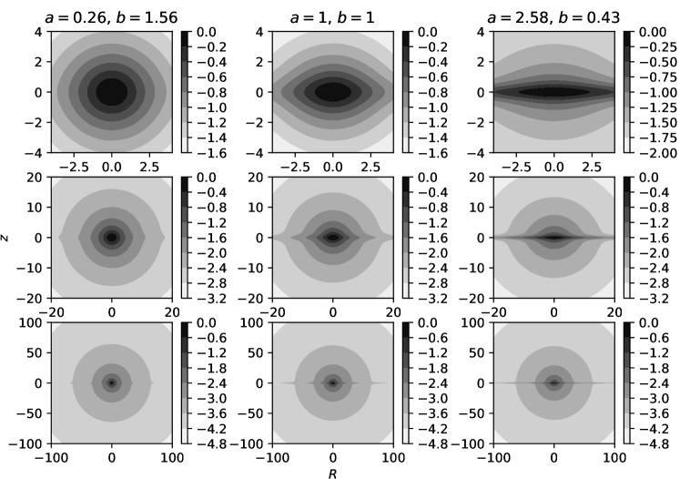
where $s^{2}=R^{2}+(a+\!\sqrt{z^{2}+b^{2}})^{2}$ with the scale constant replace by $\Phi_{0}\to\varv_{\infty}^{2}$. Figure 1 shows some examples for the isodensity contours of this case. As the asymptotic fall-off of the density is like $\sim s^{-2}\sim R^{-2}\sim z^{-2}$, this model may be considered as a “flattened isothermal” model. Note that the circular speed behaves like

$$\varv_{\mathrm{c}}^{2}=R\frac{\partial\Phi}{\partial R}=\frac{\varv_{\infty}^{2}R^{2}}{R^{2}+(a+z_{b})^{2}}\stackrel{{\scriptstyle z=0}}{{\Longrightarrow}}\varv_{\infty}^{2}\left(1-\frac{(a+b)^{2}}{R^{2}+(a+b)^{2}}\right),$$ (26)

which actually is identical to that of the so-called logarithmic potential of Binney (Binney & Tremaine, 2008, sect. 2.3.2). In fact, the $a=0$ limit of the current model is the same as the spherical limit for Binney’s potential (or the softened isothermal sphere; eq. 2.12 of Evans, 1993)

$$\rho^{\rm MN}=\frac{\varv_{\infty}^{2}}{4\pi G(r^{2}+b^{2})}\left(1+\frac{2b^{2}}{r^{2}+b^{2}}\right);\quad\Phi=\frac{\varv_{\infty}^{2}}{2}\ln\left(1+\frac{r^{2}}{b^{2}}\right).$$ (27)

Unlike Binney’s potential however, the isothermal sphere flattened according to the Miyamoto–Nagai scheme is always non-negative and better behaved for a much wider range of axis-ratios, although the equipotentials are not spheroidal any more.

Figure 2: Density profiles along the one-dimensional radial ray of the flattened isothermal model with $a=b=1$. The solid line is along the major axis (on the plane) and the dashed line is along the minor axis (on the symmetry axis). Also shown are the behaviours along some inclined directions: the latitudes of 0°($=$ along the major axis), 30°, 45°, 60°, and 90°($=$ along the minor axis). As the isodensity surfaces are “oblate,” the density decrease with the increasing latitude at the same radius. Note that the density decays noticeably slower on the plane than along the directions off plane.

Near the origin, we find that

$$\rho^{\rm MN}\simeq\frac{\varv_{\infty}^{2}}{4\pi Gb(a+b)^{2}}\\ \times\left[a+3b-\frac{a+5b}{(a+b)^{2}}R^{2}-\frac{3a^{2}+9ab+10b^{2}}{2b^{2}(a+b)}z^{2}+\cdots\right],$$ (28)

and so the axis ratio of the isodensity surface approaches to

$$\frac{R_{0}}{z_{0}}=\!\sqrt{1+\frac{\chi(17+12\chi+3\chi^{2})}{2(5+\chi)}},$$ (29)

as $R,z\to 0$, where $\chi=a/b$. On the other hand, the asymptotic behaviours of the density profile are found to be

$$\begin{split}\rho^{\rm MN}&\simeq\frac{\varv_{\infty}^{2}}{4\pi G}\left(1+\frac{ab^{2}}{z_{b}^{3}}\right)\frac{1}{R^{2}}+\mathcal{O}(R^{-4})\quad(R\to\infty),\\ \rho^{\rm MN}&\simeq\frac{\varv_{\infty}^{2}}{4\pi G}\frac{1}{z^{2}}+\mathcal{O}(z^{-3})\quad(z\to\infty).\end{split}$$ (30)

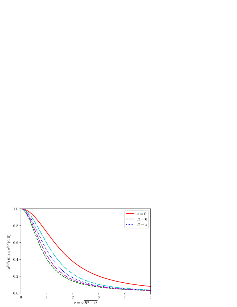
If $z=0$, then $z_{b}=b$ and so the axis ratio of the isodensity surface asymptotically tends to $\to(1+a/b)^{1/2}\geq 1$, which is closer to the unity than the limiting value at equation (29) for all $\chi>0$. However according to Figure 1, the shapes of the isodensity surfaces at large radii are actually ”Saturn-like” (that is, a disk or ring on top of a sphere). Similarly the density fall-offs of the model with $a=b=1$ shown in Figure 2 also indicate the decay along the minor axis is noticeably slower than those along the directions off plane (all of which tend to a common behaviour implying approximate sphericity). This is understood from the fact that, if $z/R\neq 0$ is fixed, we have $z\to\infty$ and so $ab^{2}/z_{b}^{3}\to 0$ as $R\to\infty$.

Lastly, the $b=0$ limit of the family is given by

$$\begin{split}\rho^{\rm MN}&=\frac{\varv_{\infty}^{2}}{4\pi G}\frac{1}{R^{2}+(a+|z|)^{2}}+\frac{\varv_{\infty}^{2}}{2\pi G}\frac{a\deltaup(z)}{R^{2}+a^{2}};\\ \Phi^{\rm MN}&=\frac{\varv_{\infty}^{2}}{2}\ln\left(\frac{R^{2}+(a+|z|)^{2}}{a^{2}}\right).\end{split}$$ (31)

The flat rotation curve here is actually due to the displaced singular isothermal sphere part, and not to the razor-thin disk component, which falls like $\sim R^{-2}$ as $R\to\infty$ and may be considered as the model-$\frac{1}{2}$ of the Toomre (1963) disk. We also note that the potential due to the razor-thin disk component alone actually requires an elliptic integral (of the elliptic/spheroidal coordinates) to write down (Evans & de Zeeuw, 1992, Table 3, $m=1$), but the superposed potential of the current model only involves elementary functions of the cylindrical coordinate components.

4.2 Hypervirial Models

In order to obtain a model with a finite total mass, we need to start with a spherical model with $\Phi^{\mathrm{s}}\sim r^{-1}$ as $r\to\infty$. One such possibility is provided by the hypervirial models of Evans & An (2005) (also known as the Veltmann (1979) isochronous spheres)

$$\begin{split}\Phi^{\mathrm{s}}(r)&=-\frac{GM}{(r^{p}+c^{p})^{1/p}};\\ \bar{\rho}^{\mathrm{s}}(r)&=\frac{3M}{4\pi}\frac{1}{r^{2-p}(r^{p}+c^{p})^{1/p+1}};\\ \rho^{\mathrm{s}}(r)&=\frac{M}{4\pi}\frac{(p+1)\,c^{p}}{r^{2-p}(r^{p}+c^{p})^{1/p+2}}.\end{split}$$ (32)

After the substitution, the density profile is then given by

$$\rho^{\rm MN}=\frac{M}{4\pi s^{2-p}(s^{p}+c^{p})^{1/p+1}}\\ \times\left[\frac{ab^{2}}{(z^{2}+b^{2})^{3/2}}+\frac{(p+1)\,c^{p}}{s^{p}+c^{p}}+\frac{b^{2}h^{2}}{z^{2}+b^{2}}\frac{3s^{p}+(2-p)\,c^{p}}{s^{2}(s^{p}+c^{p})}\right]$$ (33)

which is nonnegative for $p\leq 2$. Here if $c=0$, the model reproduces the Miyamoto–Nagai disk independent of $p$. If $c>0$, the density falls off asymptotically like $\rho^{\rm MN}\sim R^{-3}$ along the major axis ($z=0$), whilst, along the minor axis ($R=0$), we find $\rho^{\rm MN}\sim z^{-(p+3)}$.

If $p=2$, we have some simplifications for $s^{p}+c^{p}=s^{2}+c^{2}=r^{2}+a^{2}+b^{2}+c^{2}+2a\!\sqrt{z^{2}+b^{2}}=\mathcal{S}^{2}$ and so

$$\rho^{\rm MN}=\frac{M}{4\pi\mathcal{S}^{3}}\\ \times\Biggl{[}\frac{ab^{2}}{(z^{2}+b^{2})^{3/2}}+\left(\frac{a^{2}b^{2}}{z^{2}+b^{2}}+\frac{2ab^{2}}{\!\sqrt{z^{2}+b^{2}}}+b^{2}+c^{2}\right)\frac{3}{\mathcal{S}^{2}}\Biggr{]}.$$ (34)

Notably if $b^{2}+c^{2}\geq 0$, this is still nonnegative everywhere. In particular, if we choose $c^{2}=-b^{2}$, this model reduces to

$$\rho^{\rm MN}=\frac{ab^{2}M}{4\pi\mathcal{S}^{3}}\left[\frac{1}{(z^{2}+b^{2})^{3/2}}+\left(\frac{a}{z^{2}+b^{2}}+\frac{2}{\!\sqrt{z^{2}+b^{2}}}\right)\frac{3}{\mathcal{S}^{2}}\right],$$ (35)

where $\mathcal{S}^{2}=s^{2}+c^{2}=s^{2}-b^{2}=r^{2}+a^{2}+2a\!\sqrt{z^{2}+b^{2}}\geq 0$. It turns out that this is equivalent to equation (8) of the Satoh (1980), who arrived at the same model via a somewhat roundabout route. Also note that the minor-axis asymptotic density fall-off of the Satoh disk is steeper like $\sim z^{-6}$ than all other cases ($b^{2}+c^{2}>0$) of equation (34), for which $\rho^{\rm MN}\sim z^{-5}$.

Figure 3: Same as Figure 1 except for the density profiles in equation (45) with $r_{0}=(a+b)/\mathrm{e}^{1/3}$.

5 Cosmological Halo Models

So far, we have exploited the Miyamoto–Nagai substitution to provide models with asymptotic density fall-off like $R^{-2}$ or $z^{-2}$ (the flattened isothermal model), or like $R^{-3}$ along the major axis and $z^{-5}$ or steeper along the minor axis (the flattened hypervirial models including Satoh’s model). Cosmological simulations suggest that dark haloes may have densities that decay like distance^-3 (Navarro et al., 1997). It would be interesting to find flattened models with this property. To do this, we first study the asymptotic behaviour of models under the Miyamoto–Nagai substitution.

5.1 Asymptotic Behaviour

If the initial spherical model has finite total mass and the enclosed mass approaches it like $M^{\mathrm{s}}(r)\simeq m_{0}-m_{1}(r/r_{0})^{-\nu}$ ($\nu>0$) as $r\to\infty$, we have asymptotic behaviour like $\rho^{\mathrm{s}}(r)\simeq\nu m_{1}r_{0}^{\nu}/(4\pi r^{3+\nu})$ and $\bar{\rho}^{\mathrm{s}}(r)\simeq 3m_{0}/(4\pi r^{3})$. According to equation (15), these indicate that the asymptotic density fall-offs of the model after the Miyamoto–Nagai substitution are like

$$\rho^{\rm MN}\simeq\frac{ab^{2}m_{0}}{4\pi z_{b}^{3}}\frac{1}{R^{3}};\qquad\rho^{\rm MN}\simeq\frac{\nu m_{1}r_{0}^{\nu}}{4\pi}\frac{1}{z^{3+\nu}}+\frac{3b^{2}m_{0}}{4\pi}\frac{1}{z^{5}}.$$ (36)

That is to say, along the minor axis (i.e. the $R=0$ symmetry axis), the resulting density profile falls off faster than $\sim z^{-3}$, although the density on the $z=0$ plane always decays like $\sim R^{-3}$. Instead, if we start with the model with the mass growing like $M^{\mathrm{s}}(r)\simeq m_{1}(r/r_{0})^{\xi}$ ($\xi>0$) as $r\to\infty$, we have $\rho^{\mathrm{s}}(r)\simeq\xi m_{1}/(4\pi r_{0}^{\xi}r^{3-\xi})$ and $\rho^{\mathrm{s}}(r)\simeq 3m_{1}/(4\pi r_{0}^{\xi}r^{3-\xi})$, and so the density profile after the substitution falls off with the same power index as $\rho^{\mathrm{s}}$;

$$\rho^{\rm MN}\simeq\frac{m_{1}}{4\pi r_{0}^{\xi}}\left(\xi+\frac{ab^{2}}{z_{b}^{3}}\right)\frac{1}{R^{3-\xi}};\qquad\rho^{\rm MN}\simeq\frac{\xi m_{1}}{4\pi r_{0}^{\xi}}\frac{1}{z^{3-\xi}}.$$ (37)

However, the cosmologically interesting asymptotic density fall-off of $\rho^{\mathrm{s}}\sim r^{-3}$ (e.g, Navarro et al., 1997) is actually the borderline case. Unfortunately, if we start with the corresponding mass model of $M^{\mathrm{s}}(r)\simeq m_{1}\ln(r/r_{0})$, the resulting model after the substitution exhibits asymptotic behaviour like

$$\rho^{\rm MN}\simeq\frac{m_{1}}{4\pi R^{3}}\left(1+\frac{ab^{2}}{z_{b}^{3}}\ln\frac{R}{r_{0}}\right);\qquad\rho^{\rm MN}\simeq\frac{m_{1}}{4\pi z^{3}}.$$ (38)

In other words, the asymptotic density fall-off on the plane is strictly slower than that of $\sim R^{-3}$ due to the logarithmic term (assuming $ab\neq 0$). Nevertheless, we observe that the coefficient of the $R^{-3}\ln R$ term in equation (38) is linear in $a$ whereas those of the $R^{-3}$ and $z^{-3}$ terms are independent of $a$. Hence, if we consider the model given by the difference of $\Phi^{\mathrm{s}}[\!\sqrt{R^{2}+(na+z_{b})^{2}}]$ and $n\Phi^{\mathrm{s}}[\!\sqrt{R^{2}+(a+z_{b})^{2}}]$ where $z_{b}^{2}=z^{2}+b^{2}$ and $\Phi^{\mathrm{s}}(r)$ is the potential due to a spherical density profile with the asymptotic behaviour like $\sim r^{-3}$, it is expected that the resulting density profile behaves asymptotically like both $\sim R^{-3}$ and $\sim z^{-3}$.

Figure 4: Same as Figure 1 except for the density profiles in equation (51) with $r_{0}=(a+b)/\mathrm{e}^{8/15}$.

5.2 The difference models with different $a$

From equation (15) and $\mathrm{d}\bar{\rho}^{\mathrm{s}}/\mathrm{d}r=3(\rho^{\mathrm{s}}-\bar{\rho}^{\mathrm{s}})/r$, we find that

$$\frac{\mathrm{d}}{\mathrm{d}a}\!\left(\frac{\rho^{\rm MN}}{a}\right)=\frac{R^{2}z_{b}^{2}+z^{2}h^{2}}{az_{b}^{2}s^{2}}\frac{h}{s}\frac{\mathrm{d}\rho^{\mathrm{s}}(s)}{\mathrm{d}s}-\frac{\rho^{\mathrm{s}}(s)}{a^{2}}\\ -\frac{b^{2}h}{az_{b}^{2}}\left[1+\frac{(a-z_{b})^{2}}{az_{b}}+\frac{5h^{2}}{s^{2}}\right]\frac{\bar{\rho}^{\mathrm{s}}(s)-\rho^{\mathrm{s}}(s)}{s^{2}},$$ (39)

which is negative provided that $\mathrm{d}\rho^{\mathrm{s}}/\mathrm{d}r\leq 0$ (and $a>0$). That is to say, we have $\rho^{\rm MN}\approx Ca^{\lambda}$ locally with $\lambda=\mathrm{d}\ln\rho^{\rm MN}/\mathrm{d}\ln a<1$, and so $\rho^{\rm MN}$ with $a\to na$ is smaller than the $n$-times multiple of $\rho^{\rm MN}$ – i.e. $C(na)^{\lambda}=n^{\lambda}\rho^{\rm MN}<n\rho^{\rm MN}$ – for $n>1$. It follows that, if $\Phi^{\mathrm{s}}(r)$ is the potential due to a positive radially non-increasing spherical density profile, then the function (where $n>1$ and $z_{b}^{2}=z^{2}+b^{2}$)

$$\Phi^{\mathrm{d}}_{n}(R,z)=\frac{n\Phi^{\mathrm{s}}[\!\sqrt{R^{2}+(a+z_{b})^{2}}]-\Phi^{\mathrm{s}}[\!\sqrt{R^{2}+(na+z_{b})^{2}}]}{n-1}$$ (40)

is that of an axisymmetric non-negative density profile, $\rho^{\mathrm{d}}_{n}(R,z)$, which may be found directly via the Poisson equation or utilizing equation (15) with appropriate substitutions. Furthermore, if the asymptotic behaviour of the original spherical density profile is power-law-like, as in $\rho^{\mathrm{s}}/\rho_{0}\simeq(r/r_{0})^{-\nu}$ with $\nu<5$, then the asymptotic behaviour of the resulting density profile also follows that like $\rho^{\mathrm{d}}_{n}/\rho_{0}\simeq(R/r_{0})^{-\nu}$ and $\simeq(z/r_{0})^{-\nu}$ along both major and minor axes (the isodensity surfaces also becomes spherical in large radii). If $\nu>5$ on the other hand, the asymptotic behaviour saturates at $\sim R^{-5}$ and $\sim z^{-5}$ with

$$\rho^{\mathrm{d}}_{n}\simeq\frac{3b^{2}m_{0}}{4\pi R^{5}}\left(1+\frac{n(n+1)a^{3}}{2z_{b}^{3}}\right);\quad\rho^{\mathrm{d}}_{n}\simeq\frac{3b^{2}m_{0}}{4\pi z^{5}},$$ (41)

where $m_{0}$ is the total mass of the initial spherical model. As for the $\nu=5$ case, the terms like equation (41) and $\simeq\rho_{0}(r/R_{0})^{-5}$ are of the same order and are simply added together. For instance, if the difference model $\rho^{\mathrm{d}}_{n}=n\rho^{\rm MN}(a)-\rho^{\rm MN}(na)$ is based on $\rho^{\rm MN}$ of equation (34), the asymptotic behaviour of $\rho^{\mathrm{d}}_{n}$ is found to be

$$\rho^{\mathrm{d}}_{n}\simeq\frac{3M}{4\pi R^{5}}\left(b^{2}+c^{2}+\frac{n(n+1)a^{3}b^{2}}{2z_{b}^{3}}\right);\quad\rho^{\mathrm{d}}_{n}\simeq\frac{3(b^{2}+c^{2})M}{4\pi z^{5}},$$ (42)

whilst $\rho^{\mathrm{s}}\simeq 3c^{2}M/(4\pi r^{5})$.

5.3 The differentiation model

Given that equation (39) is always negative and the derivatives are linear, if we consider the function given by

$$\begin{split}\Phi^{\mathrm{d}}_{1}(R,z)&=-a^{2}\frac{\mathrm{d}}{\mathrm{d}a}\frac{\Phi^{\mathrm{s}}[\!\sqrt{R^{2}+(a+z_{b})^{2}}]}{a}\\ &=\Phi^{\mathrm{s}}(s)-\frac{a(a+z_{b})}{\!\sqrt{R^{2}+(a+z_{b})^{2}}}\frac{\mathrm{d}\Phi^{\mathrm{s}}(s)}{\mathrm{d}s},\end{split}$$ (43)

where $\Phi^{\mathrm{s}}(r)$ is again a potential of a spherical density profile, it becomes the potential due to the axisymmetric density profile of $\rho^{\mathrm{d}}_{1}(R,z)=-a^{2}(\mathrm{d}/\mathrm{d}a)(\rho^{\rm MN}/a)$ where $\rho^{\rm MN}$ corresponds to the density profile for $\Phi^{\mathrm{s}}[\!\sqrt{R^{2}+(a+z_{b})^{2}}]$ (eq. 15). Thanks to equation (39), $\rho^{\mathrm{d}}_{1}$ is non-negative if $\Phi^{\mathrm{s}}(r)$ is a potential due to a positive radially non-increasing density profile. In addition, the $a=0$ limit of the model simply results in the same $a=0$ limit of $\rho^{\rm MN}$. In fact, this model is the $n=1$ limit of the difference model discussed, the fact of which can be proven by taking the limit of equation (40) as $n\to 1$ by means of L’Hôpital’s rule. Then the asymptotic behaviour of the density profile is given by the same $n=1$ limit of the preceding discussion, namely, $\rho^{\mathrm{d}}_{1}\sim R^{-\min(5,\nu)}$ and $\sim z^{-\min(5,\nu)}$ if we start with $\rho^{\mathrm{s}}\sim r^{-\nu}$.

Figure 5: Density profiles along the major and minor axes for the models in eqs (45) and (51). For both cases, $a=2.58$ and $b=0.43$ but $r_{0}=\mathrm{e}^{-1/3}(a+b)\approx 2.157$ for eq. 45 and $r_{0}=\mathrm{e}^{-1/3}(a+b)\approx 1.766$ for eq. 51.

5.4 Models with the $\sim r^{-3}$ density fall-offs

If we starts with the potential of any spherical density profile that falls off like $\sim r^{-3}$ as $r\to\infty$, the procedure outlined so far will provided us with an analytic potential–density pair for a “flattened” axisymmetric system (becoming rounder at large radii) with the asymptotic behaviour like $\sim R^{-3}$ and $\sim z^{-3}$. Every calculation required to find the explicit expressions for the potential–density pair is purely algebraic (including differentiation) provided that the starting potential is also an algebraic function. That is to say, it is possible to get a flattened density profile falling off like $\sim r^{-3}$ whose potential is also expressible only using algebraic functions of the cylindrical coordinates if we start with the potential for density profiles of the form $\rho^{\mathrm{s}}\propto 1/[r^{\alpha}(c^{p}+r^{p})^{(3-\alpha)/p}]$ with $p=1,2$ and $\alpha=0,1,2$ (An & Zhao, 2013) including the NFW profile ($\alpha=p=1$; Navarro et al., 1997) for which $\Phi^{\mathrm{s}}(r)\propto-\ln(1+r/c)/r$. However, the expressions do become rather unwieldy, although their numerical implementations would be, if tedious, trivial.

We prefer to begin with a starting potential as simple as possible: consider the function

$$\begin{split}\Phi^{\mathrm{s}}(r)&=-\frac{\Phi_{0}r_{0}}{r}\left[\ln\left(\frac{r}{r_{0}}\right)+1\right];\quad\frac{\mathrm{d}\Phi^{\mathrm{s}}}{\mathrm{d}r}=\frac{\Phi_{0}r_{0}}{r^{2}}\ln x\\ \rho^{\mathrm{s}}(r)&=\frac{\Phi_{0}r_{0}}{4\pi Gr^{3}};\quad\bar{\rho}^{\mathrm{s}}(r)=\frac{3\Phi_{0}r_{0}}{4\pi Gr^{3}}\ln x;\quad\frac{\mathrm{d}\rho^{\mathrm{s}}(r)}{\mathrm{d}r}=-\frac{3\Phi_{0}r_{0}}{4\pi Gr^{4}}\end{split}$$ (44)

where $x=r/r_{0}$. This is not a physical potential since the $r^{-3}$-cusp is not integrable (and also $\bar{\rho}<0$ for $x<1$ as well as $\bar{\rho}<\rho$ for $x<\mathrm{e}^{1/3}$). Nonetheless, this is immaterial for our purpose because the Miyamoto–Nagai substitution smears out the unphysical properties. Equation (15) is still valid for the density profile after the Miyamoto–Nagai substitution, and so we first arrive at the potential–density pair of the form

$$\begin{split}\Phi^{\rm MN}(R,z)&=-\frac{\Phi_{0}r_{0}}{s}\left(1+\frac{1}{2}\ln\frac{s^{2}}{r_{0}^{2}}\right)\\ \rho^{\rm MN}(R,z)&=\frac{\Phi_{0}r_{0}}{4\pi Gs^{5}}\Biggl{(}R^{2}+\frac{z^{2}(a+z_{b})^{2}}{z_{b}^{2}}\\ &\qquad+b^{2}\frac{aR^{2}+(a+3z_{b})(a+z_{b})^{2}}{z_{b}^{3}}\ln\frac{s}{r_{0}}\Biggr{)}\end{split}$$ (45)

where $z_{b}^{2}=z^{2}+b^{2}$ and $s^{2}=R^{2}+(a+z_{b})^{2}$, with the limiting cases;

$$\begin{split}\rho^{\rm MN}&\stackrel{{\scriptstyle a=0}}{{=}}\frac{\Phi_{0}r_{0}}{4\pi G}\frac{R^{2}+z^{2}+3b^{2}\ln(r_{b}/r_{0})}{(R^{2}+z^{2}+b^{2})^{5/2}}\\ \rho^{\rm MN}&\stackrel{{\scriptstyle b=0}}{{\Rightarrow}}\frac{\Phi_{0}r_{0}}{4\pi G}\left[\frac{1}{[R^{2}+(a+|z|)^{2}]^{3/2}}+2\deltaup(z)\frac{a\ln(R_{a}/r_{0})}{(R^{2}+a^{2})^{3/2}}\right]\end{split}$$ (46)

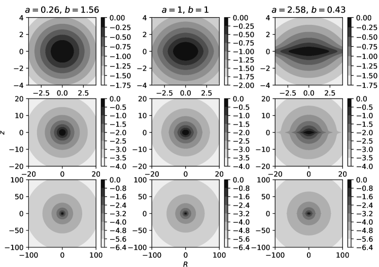
where $R_{a}^{2}=R^{2}+a^{2}$ and $r_{b}^{2}=R^{2}+z^{2}+b^{2}$. In Figure 3, we have also shown some examples of the isodensity contours due to the density profile in equation (45). This model may be considered as an alternative $\xi=3$ limit of the power-law model discussed in Sect. 4.1. In addition we find that $R^{-1}\partial\rho^{\rm MN}(R,z)/\partial R=-A-b^{2}B[3\ln(s/r_{0})-1]$ and $z^{-1}\partial\rho^{\rm MN}(R,z)/\partial z=-C-b^{2}D[3\ln(s/r_{0})-1]$ where $(A,B,C,D)$ are some non-negative algebraic functions of $(R,z,a,b)$ and so $r_{0}\leq(a+b)\,\mathrm{e}^{-1/3}\approx 0.7165(a+b)$ is a sufficient condition for the density profile to be non-negative and outwardly decreasing. Near the origin, the density simply behaves like

$$\rho^{\rm MN}\simeq\frac{\Phi_{0}r_{0}}{4\pi Gb(a+b)^{3}}\left[(a+3b)\ln x_{0}-\frac{1}{2}\left(\frac{R^{2}}{R_{0}^{2}}+\frac{z^{2}}{z_{0}^{2}}\right)+\cdots\right],$$ (47)

where $x_{0}=(a+b)/r_{0}$ and

$$\begin{split}\frac{1}{R_{0}^{2}}&=\frac{(a+5b)(3\ln x_{0}-1)}{(a+b)^{2}};\\ \frac{1}{z_{0}^{2}}&=\frac{1}{b^{2}}\left[a+\frac{a^{2}+4ab+5b^{2}}{a+b}(3\ln x_{0}-1)\right],\end{split}$$ (48)

whereas the asymptotic behaviours are like

$$\begin{split}\rho^{\rm MN}&\simeq\frac{\Phi_{0}r_{0}}{4\pi GR^{3}}\left(1+\frac{ab^{2}\ln(R/r_{0})}{(z^{2}+b^{2})^{3/2}}\right)+\mathcal{O}(R^{-5}\ln R)&(R\to\infty);\\ \rho^{\rm MN}&\simeq\frac{\Phi_{0}r_{0}}{4\pi Gz^{3}}\left(1-\frac{3a}{z}\right)+\mathcal{O}(z^{-5}\ln z)&(z\to\infty).\end{split}$$ (49)

Finally, equation (43) based on this model then results in

$$\Phi^{\mathrm{d}}_{1}(R,z)=-\frac{\Phi_{0}r_{0}}{s}\left(1+\frac{1}{2}\frac{R^{2}+(2a+z_{b})(a+z_{b})}{R^{2}+(a+z_{b})^{2}}\ln\frac{s^{2}}{r_{0}^{2}}\right)$$ (50)

and the corresponding density profile becomes

$$\rho^{\mathrm{d}}_{1}(R,z)=\frac{\Phi_{0}r_{0}}{4\pi G}\Biggl{\{}\frac{1}{s^{3}}+\frac{3a(a+z_{b})}{s^{5}}\frac{R^{2}z_{b}^{2}+z^{2}(a+z_{b})^{2}}{z_{b}^{2}s^{2}}\\ +\frac{ab^{2}(a+z_{b})}{z_{b}^{2}s^{5}}\left[1+\frac{(a-z_{b})^{2}}{az_{b}}+\frac{5(a+z_{b})^{2}}{s^{2}}\right]\left(3\ln\frac{s}{r_{0}}-1\right)\Biggr{\}}$$ (51)

with the $b=0$ limit being

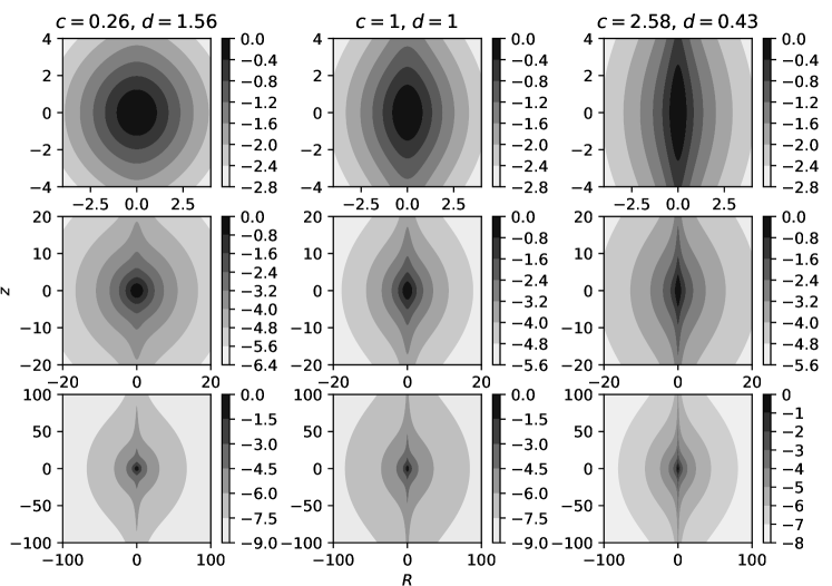
$$\rho^{\mathrm{d}}_{1}(R,z)\stackrel{{\scriptstyle b=0}}{{\Rightarrow}}\frac{\Phi_{0}r_{0}}{4\pi G}\Biggl{\{}\frac{R^{2}+(4a+|z|)(a+|z|)}{[R^{2}+(a+|z|)^{2}]^{5/2}}\\ +2\deltaup(z)\frac{a^{3}[3\ln(R_{a}/r_{0})-1]}{(R^{2}+a^{2})^{5/2}}\Biggr{\}}.$$ (52)

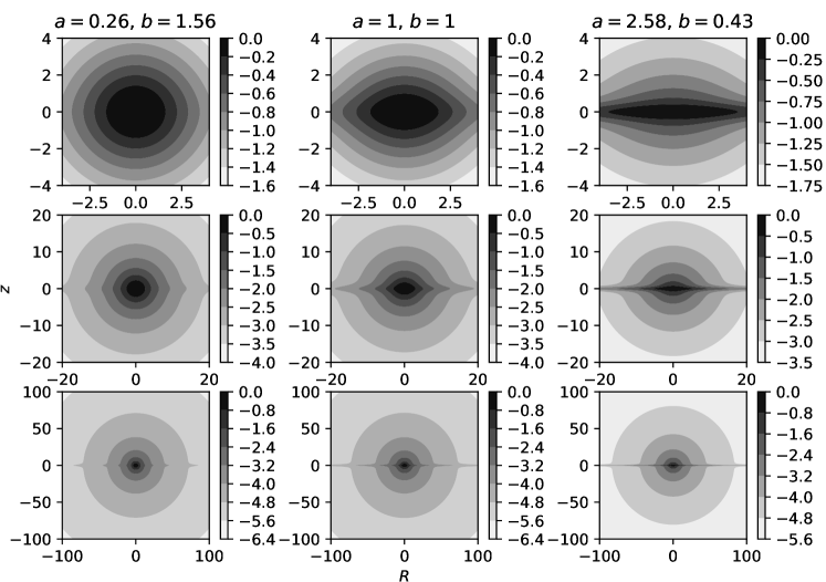
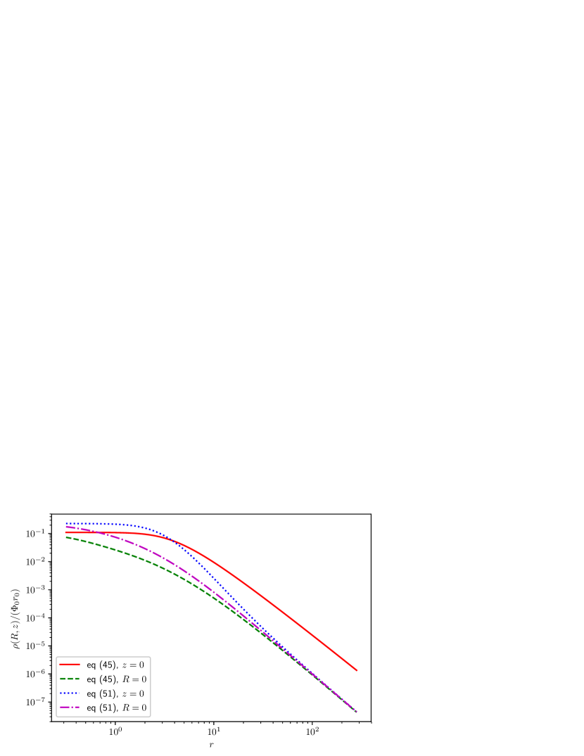
Figure 4 shows some example isodensity contours resulting from equation (51), whilst Figure 5 illustrates the behaviours of the density along the major and minor axes for a particular case. Since the model is specifically constructed in such a way, the asymptotic behaviours of the density are indeed given by

$$\rho^{\mathrm{d}}_{1}\simeq\frac{\Phi_{0}r_{0}}{4\pi GR^{3}}+\mathcal{O}(R^{-5}\ln R);\quad\rho^{\mathrm{d}}_{1}\simeq\frac{\Phi_{0}r_{0}}{4\pi Gz^{3}}+\mathcal{O}(z^{-5}\ln z),$$ (53)

whereas the Taylor–Maclaurin series is

$$\rho^{\mathrm{d}}_{1}\simeq\frac{\Phi_{0}r_{0}}{4\pi G(a+b)^{3}}\Biggl{[}1+\frac{a^{2}+4ab+b^{2}}{b(a+b)}L_{3}\\ \hfill-\frac{3(3a^{3}+5b^{3})+(3a^{3}+15a^{2}b+25ab^{2}+5b^{3})L_{15/8}}{10b^{3}(a+b)^{2}}z^{2}\\ -\left(3+\frac{a^{2}+6ab+b^{2}}{b(a+b)}L_{15/8}\right)\frac{R^{2}}{2(a+b)^{2}}+\cdots\Biggr{]},$$ (54)

where $L_{3}=3\ln[(a+b)/r_{0}]-1$ and $L_{15/8}=15\ln[(a+b)/r_{0}]-8$. This last series also implies that the density profile might be increasing near the origin if $(a+b)/r_{0}$ is chosen too small, but the examinations of $\partial\rho^{\mathrm{d}}_{1}/\partial R$ and $\partial\rho^{\mathrm{d}}_{1}/\partial z$ indicate that $r_{0}\leq(a+b)\mathrm{e}^{-8/15}\approx 0.5866(a+b)$ is actually sufficient to guarantee the positive non-increasing density profile.

Figure 6: Same as Figure 1 except for the density profiles in equation (64).

6 The Prolate and Triaxial Substitutions

One possible generalization of the Miyamoto–Nagai substitution is applying a similar transformation to the other coordinates. For instance, consider the transformation of a spherical function $\Phi^{\mathrm{s}}(r)$ to $\Phi^{\rm gMN}(R,z)=\Phi^{\mathrm{s}}(t)$ where $t^{2}=(c+R_{d})^{2}+(a+z_{b})^{2}$ and $(R_{d}^{2},z_{b}^{2})=(R^{2}+d^{2},z^{2}+b^{2})$. With $\Phi^{\rm gMN}(R,z)$ as the potential, the resulting gravity field is given by $\mn@boldsymbol{\varg}=-\mn@boldsymbol{\nabla}\Phi^{\rm gMN}=-(\mn@boldsymbol{\nabla}t)GM^{\mathrm{s}}(t)/t^{2}$ with

$$t(\mn@boldsymbol{\nabla}t)=\left(1+\frac{c}{R_{d}}\right)R\hat{\mn@boldsymbol{e}}_{R}+\left(1+\frac{a}{z_{b}}\right)z\Bbbk.$$ (55)

The gravitational force points locally to a more vertically inclined direction than that to the centre if $a/z_{b}>c/R_{d}$ and vice versa, whilst it points radially towards the centre everywhere (i.e. the spherical potential) if $a=c=0$. The equipotential in the limit of $R,z\to 0$ is oblate if $a/b>c/d$ or prolate if $c/d>a/b$, whereas the equipotentials as $R,z\to\infty$ become spherical. If $d=0$ and $c\neq 0$, we also find $\partial t/\partial R$ is non-zero finite and so the gravitational force becomes undifferentiable along any path that crosses the symmetry axis. This behaviour is understood from the fact that the corresponding density profiles are singular in this limit (like $\sim R^{-1}$) on the $R=0$ axis.

The Poisson equation indicates that the axisymmetric density profile generating the potential $\Phi^{\mathrm{s}}(t)$ can be expressed as

$$\rho^{\rm gMN}(R,z)=\frac{\nabla^{2}\Phi^{\mathrm{s}}(t)}{4\pi G}=\rho^{\mathrm{s}}(t)+\left[\frac{ab^{2}}{z_{b}^{3}}+\frac{c(R^{2}+2d^{2})}{R_{d}^{3}}\right]\frac{\bar{\rho}^{\mathrm{s}}(t)}{3}\\ +\left[\frac{b^{2}(a+z_{b})^{2}}{z_{b}^{2}}+\frac{d^{2}(c+R_{d})^{2}}{R_{d}^{2}}\right]\frac{\bar{\rho}^{\mathrm{s}}(t)-\rho^{\mathrm{s}}(t)}{t^{2}},$$ (56)

generalizing equation (15), which corresponds to the $c=d=0$ case. It is easy to observe that this density profile is also always non-negative if $\bar{\rho}^{\mathrm{s}}(r)\geq\rho^{\mathrm{s}}(r)\geq 0$ (actually $\rho^{\mathrm{s}}(r)$ being non-negative and integrable at $r=0$ is sufficient), and, from explicit calculation, we can furthermore demonstrate that $\partial\rho^{\rm gMN}/\partial R\leq 0$ and $\partial\rho^{\rm gMN}/\partial z\leq 0$ if $(\rho^{\mathrm{s}})^{\prime}(r)\leq 0$ (and $\bar{\rho}^{\mathrm{s}}(r)\geq\rho^{\mathrm{s}}(r)\geq 0$).

Since $t\geq t_{0}=\!\sqrt{(a+b)^{2}+(c+d)^{2}}\geq 0$, eqn (56) is also regular everywhere with the Taylor-MacLaurin series is

$$\frac{\rho^{\rm gMN}(R,z)}{\bar{\rho}^{\mathrm{s}}(t_{0})}\simeq 1+\frac{a}{3b}+\frac{2c}{3d}-\frac{1}{2}\left(\frac{R^{2}}{R_{0}^{2}}+\frac{z^{2}}{z_{0}^{2}}\right)+\cdots$$ (57)

unless $bd=0$. Here,

$$\begin{split}\frac{b^{2}}{z_{0}^{2}}&=\frac{a}{b}+\frac{(a+b)(3ad+2bc+5bd)}{dt_{0}^{2}}\frac{\bar{\rho}^{\mathrm{s}}(t_{0})-\rho^{\mathrm{s}}(t_{0})}{\bar{\rho}^{\mathrm{s}}(t_{0})};\\ \frac{d^{2}}{R_{0}^{2}}&=\frac{4c}{3d}+\frac{(c+d)(ad+4bc+5bd)}{bt_{0}^{2}}\frac{\bar{\rho}^{\mathrm{s}}(t_{0})-\rho^{\mathrm{s}}(t_{0})}{\bar{\rho}^{\mathrm{s}}(t_{0})}.\end{split}$$ (58)

If $d=0$ on the other hand, equation (56) reduces to

$$\rho^{\rm gMN}=\rho^{\mathrm{s}}(t)+\left(\frac{ab^{2}}{z_{b}^{3}}+\frac{c}{R}\right)\frac{\bar{\rho}^{\mathrm{s}}(t)}{3}+\frac{b^{2}(a+z_{b})^{2}}{z_{b}^{2}}\frac{\bar{\rho}^{\mathrm{s}}(t)-\rho^{\mathrm{s}}(t)}{t^{2}},$$ (59)

which exhibits an explicit $R^{-1}$-density singularity as $R\to 0$ (i.e. the density along the symmetry axis diverges). This contrasts to the $b=0$ case, for which a razor-thin disk develops.

6.1 The Miyamoto–Nagai spindle

The simplest potential–density pair that results from this transformation is that due to the point mass potential $\Phi^{\mathrm{s}}(r)=-GM/r$; viz.

$$\Phi^{\rm gMN}=-\frac{GM}{\bigl{[}(c+\!\sqrt{R^{2}+d^{2}})^{2}+(a+\!\sqrt{z^{2}+b^{2}})^{2}\bigr{]}^{1/2}};$$ (60)

$$\rho^{\rm gMN}=\frac{M}{4\pi t^{3}}\Biggl{[}\frac{ab^{2}}{(z^{2}+b^{2})^{3/2}}+\frac{c(R^{2}+2d^{2})}{(R^{2}+d^{2})^{3/2}}\\ +\frac{3}{t^{2}}\left(\frac{b^{2}(a+\!\sqrt{z^{2}+b^{2}})^{2}}{z^{2}+b^{2}}+\frac{d^{2}(c+\!\sqrt{R^{2}+d^{2}})^{2}}{R^{2}+d^{2}}\right)\Biggr{]},$$ (61)

where $t^{2}=(c+\!\sqrt{R^{2}+d^{2}})^{2}+(a+\!\sqrt{z^{2}+b^{2}})^{2}$. Obviously, the $c=d=0$ case reduces to the Miyamoto–Nagai disk (or the Kuzmin disk if $b=c=d=0$), whereas the $a=c=0$ case results in the Plummer sphere, i.e. $\rho^{\rm gMN}\propto(r^{2}+b^{2}+d^{2})^{-5/2}$. If $b=0$ and $a\neq 0$, the proper density model should additionally include the razor-thin disk on the $z=0$ midplane with the surface density $\sigma(R)$ of

$$\sigma=\frac{aM}{2\pi\bigl{[}(c+\!\sqrt{R^{2}+d^{2}})^{2}+a^{2}\bigr{]}^{3/2}}.$$ (62)

By contrast, if $d=0$ and $c\neq 0$, eqn (61) contains the $R^{-1}$ singular component – $cM/(4\pi Rt^{3})$ – in it, and with the simplest case that $a=b=d=0$ and $c\neq 0$, only such a component remains:

$$\Phi^{\rm gMN}=-\frac{GM}{\!\sqrt{(c+R)^{2}+z^{2}}};\quad\rho^{\rm gMN}=\frac{cM}{4\pi R[(c+R)^{2}+z^{2}]^{3/2}}.$$ (63)

In Fig. 6, we present the contour plots for some examples of the pure spindle-like cases (viz. $a=b=0$) given by

$$\begin{split}\Phi^{\rm gMN}&=-\frac{GM}{\bigl{[}(c+\!\sqrt{R^{2}+d^{2}})^{2}+z^{2}\bigr{]}^{1/2}};\\ \rho^{\rm gMN}&=\frac{M}{4\pi t^{3}(R^{2}+d^{2})}\Biggl{[}\frac{c(R^{2}+2d^{2})}{\!\sqrt{R^{2}+d^{2}}}+\frac{3d^{2}(c+\!\sqrt{R^{2}+d^{2}})^{2}}{t^{2}}\Biggr{]}.\end{split}$$ (64)

We observe that the contours in the central region are quite similiar to the $R$-$z$ flipped counterpart of the Miyamoto–Nagai disk, but they fall off more slowly than those for the Miyamoto–Nagai disk. The formal limit of the axis-ratio at the origin is actually found to be $(z_{0}/R_{0})^{2}=(1+\xi)(1+2\xi/3)$ where $\xi=c/d$ (which is close enough to the reciprocal of the same ratio for the Miyamoto–Nagai disk, $(R_{0}/z_{0})^{2}=(1+\chi)(5+5\chi+\chi^{2})/(5+\chi)$ where $\chi=a/b$ for a sufficiently small value of $\xi=\chi$). In addition, the contours at large radii are more prominently prolate bulge-like than the Miyamoto–Nagai disk case (resembling a sphere plus a disk). This follows from the contrasting asymptotic behaviour of the “Miyamoto–Nagai spindle,” for which $\rho^{gMN}\sim z^{-3}$ and $\rho^{gMN}\sim R^{-4}$ (cf. $\rho^{MN}\sim R^{-5}$ and $\rho^{MN}\sim z^{-3}$ for the Miyamoto–Nagai disk).

6.2 The Triaxial substitution

Instead of restricting ourselves to the axisymmetric case, we may also consider a triaxial generalization of the Miyamoto–Nagai substitution; namely, $x_{i}\to a_{i}+(x_{i}^{2}+b_{i}^{2})^{1/2}$ for all $i=1,2,3$. Whilst most of basic analyses of the models can proceed similarly as before, here we only note the counterpart to eqns (15) and (56). That is, the potential given by $\Phi(x_{1},x_{2},x_{3})=\Phi^{\mathrm{s}}(u)$ where $u^{2}=\sum_{j=1}^{3}(a_{j}+x_{b,j})^{2}$ and $x_{b,j}^{2}=x_{j}^{2}+b_{j}^{2}$ can be generated by the non-negative density profile of the form

$$\rho=\rho^{\mathrm{s}}(u)+\sum_{j=1}^{3}\frac{a_{j}b_{j}^{2}}{x_{b,j}^{3}}\frac{\bar{\rho}^{\mathrm{s}}(u)}{3}+\sum_{j=1}^{3}\frac{b_{j}^{2}(a_{j}+x_{b,j})^{2}}{x_{b,j}^{2}}\frac{\bar{\rho}^{\mathrm{s}}(u)-\rho^{\mathrm{s}}(u)}{u^{2}},$$ (65)

where $\rho^{\mathrm{s}}(r)$ and $\bar{\rho}^{\mathrm{s}}(r)$ are again the local and average density profile corresponding to the spherical potential $\Phi^{\mathrm{s}}(r)$.

7 Conclusions

This paper provides a systematic study of the Miyamoto & Nagai (1975) substitution. This is used in galactic dynamics to transform spherical potential–density pairs to flattened ones. Although introduced over forty years ago to make the ubiquitous Miyamoto & Nagai (1975) disk, the substitution does not seems to have been thoroughly scrutinized before, despite occasional model building (e.g., Satoh, 1980; Evans & Bowden, 2014).

The Miyamoto–Nagai substitution offers a number of advantages over the much more familiar practice of transforming spherical equipotentials to spheroidal or ellipsoidal ones. Specifically, if the spherical model has everywhere positive density, then the Miyamoto–Nagai substitution is guaranteed to produce a physical model. Also, after the Miyamoto–Nagai substitution, the potential retains the property that it becomes spherical at large radii, meaning that the transformed model can still have finite mass.

We have used the Miyamoto–Nagai substitution to provide some new models. First, if applied to the isothermal sphere, it yields an oblate isothermal model with an asymptotically flat rotation curve. Prolate isothernmal models can be generated by the Miyamoto-Nagai substitution applied to $R$ than than $z$. In fact, the rotation curve of these models is the same as for Binney’s logarithmic model (e.g., Evans, 1993; Binney & Tremaine, 2008), which is produced by the competing method of converting spherical equipotentials to spheroidal ones with axis ratio $q$. Binney’s model ceases to generate physical densities once $q<1/\sqrt{2}=0.707$, and so cannot become very flattened. However, our prolate or oblate flattened isothermal model is always non-negative and better behaved for a wider range of shapes.

Secondly, if we transform the hypervirial models (which includes the Plummer sphere), we obtain a highly flattened family (which includes the Satoh disk). The density along the major axis always falls like $R^{-3}$, but along the minor axis it falls much more steeply, between $z^{-3}$ and $z^{-5}$. Like the Satoh model itself, these are useful for representing very highly flattened elliptical and lenticular galaxies.

Third, we used the transformation to provide cosmological haloes, inspired by the Navarro–Frenk–White profile (Navarro et al., 1997). Here, we wish to build flattened models with simple potential–density pairs that have an asymptotic density fall-off like distance^-3. This proved to be unexpectedly hard work, but can be done by taking the difference between Miyamoto–Nagai transformed models (or equivalently, differentiating with respect to the parameters in the potential). Flattened or triaxial NFW-like models with analytic potentials are hard to construct (cf. Bowden et al., 2013, for a different method), and we plan to return to this problem in a later publication.

References

- An & Zhao (2013) An J., Zhao H., 2013, MNRAS, 428, 2805
- Binney & Tremaine (2008) Binney J., Tremaine S., 2008, Galactic Dynamics, 2nd edn. Princeton Univ. Press, Princeton NJ
- Bowden et al. (2013) Bowden A., Evans N. W., Belokurov V., 2013, MNRAS, 435, 928
- Chandrasekhar (1969) Chandrasekhar S., 1969, Ellipsoidal Figures of Equilibrium, Yale Univ. Press, New Haven CT (reprinted: 1987, Dover, New York NY)
- Evans (1993) Evans N. W., 1993, MNRAS, 260, 191
- Evans (1994) Evans N. W., 1994, MNRAS, 267, 333
- Evans & An (2005) Evans N. W., An J., 2005, MNRAS, 360, 492
- Evans & Bowden (2014) Evans N. W., Bowden A., 2014, MNRAS, 443, 2
- Evans & de Zeeuw (1992) Evans N. W., de Zeeuw P. T., 1992, MNRAS, 257, 152
- Kassiola & Kovner (1993) Kassiola A., Kovner I., 1993, ApJ, 417, 450
- Kuzmin (1953) Kuzmin G. G., 1953, Tartu Astron. Obs. Teated, 1
- Kuzmin (1956) Kuzmin G. G., 1956, Azh, 33, 27
- Lynden-Bell (1989) Lynden-Bell D., 1989, MNRAS, 237, 1099
- Mestel (1963) Mestel L., 1963, MNRAS, 126, 553
- Miyamoto & Nagai (1975) Miyamoto M., Nagai R., 1975, PASJ, 27, 533
- Nagai & Miyamoto (1976) Nagai R., Miyamoto M., 1976, PASJ, 28, 1
- Navarro et al. (1997) Navarro J. F., Frenk C. S., White S. D. M., 1997, ApJ, 490, 493
- Plummer (1911) Plummer H. C., 1911, MNRAS, 71, 460
- Routh (1892) Routh E. J., 1892, A Treatise on Analytical Statics, vol. 2. Cambridge Univ. Press, Cambridge (reprinted: 1922 & 2013)
- Satoh (1980) Satoh C., 1980, PASJ, 32, 41
- Schuster (1884) Schuster A., 1884, Rep. of the 53rd meeting of the Br. Assoc. for the Adv. of Sci.: at Southport in Sep. 1883, p.427
- Veltmann (1979) Veltmann Ü.-I. K., 1979, Azh, 56, 976 (English translation in Soviet Ast., 23, 551)
- Toomre (1963) Toomre A., 1963, ApJ, 138, 385