Cosmic Shear: Inference from Forward Models

Abstract

Density-estimation likelihood-free inference (DELFI) has recently been proposed as an efficient method for simulation-based cosmological parameter inference. Compared to the standard likelihood-based Markov Chain Monte Carlo (MCMC) approach, DELFI has several advantages: it is highly parallelizable, there is no need to assume a possibly incorrect functional form for the likelihood and complicated effects (e.g the mask and detector systematics) are easier to handle with forward models. In light of this, we present two DELFI pipelines to perform weak lensing parameter inference with lognormal realizations of the tomographic shear field – using the $C_{\ell}$ summary statistic. The first pipeline accounts for the non-Gaussianities of the shear field, intrinsic alignments and photometric-redshift error. We validate that it is accurate enough for Stage III experiments and estimate that $\mathcal{O}(1000)$ simulations are needed to perform inference on Stage IV data. By comparing the second DELFI pipeline, which makes no assumption about the functional form of the likelihood, with the standard MCMC approach, which assumes a Gaussian likelihood, we test the impact of the Gaussian likelihood approximation in the MCMC analysis. We find it has a negligible impact on Stage IV parameter constraints. Our pipeline is a step towards seamlessly propagating all data-processing, instrumental, theoretical and astrophysical systematics through to the final parameter constraints.

I Introduction

Weak lensing by large scale structure offers some of the tightest constraints on cosmological parameters. Over the next decade data from Stage IV experiments including Euclid Laureijs et al. (2010), WFIRST Spergel et al. (2015) and LSST Anthony and Collaboration will begin taking data. Extracting as much information from these ground-breaking data sets, in an unbiased way, presents a formidable challenge.

The majority of cosmic shear studies to date focus on extracting information from two-point statistics and in particular the correlation function, $\xi(\theta)$, in configuration space and the lensing power spectrum, $C_{\ell}$, in spherical harmonic space Heymans et al. (2013); Troxel et al. (2017); Kitching et al. (2014); Hildebrandt et al. (2017); Hikage et al. (2018). While the non-Gaussian information in the shear field is accessed with higher-order statistics Semboloni et al. (2010); Fu et al. (2014), peak counts Peel et al. (2017); Jain and Van Waerbeke (2000) or machine learning Gupta et al. (2018), the impact of systematics on the two-point functions have been extensively studied Massey et al. (2012). For this reason we will focus on these statistics and leave the higher-order information to a future study. In particular we focus on the $C_{\ell}$ statistic because computing correlation functions from catalogues with billions galaxies – even using an efficient code such as TREECORR Jarvis (2004) – is extremely computationally demanding.

Apart from Alsing et al. (2015a, 2016), existing studies of the shear two-point statistics Heymans et al. (2013); Troxel et al. (2017); Kitching et al. (2014); Hildebrandt et al. (2017); Hikage et al. (2018) use a Gaussian likelihood analysis to infer the cosmological parameters. This approach has drawbacks. For example, with the improved statistical precision of next generation data, we will need to propagate complicated ‘theoretical systematics’ (e.g. reduced shear Dodelson et al. (2006)) and detector effects Massey et al. (2012) into the final cosmological constraints. It is difficult to derive the expected impact of these effects as is required for a likelihood analysis. It is much easier to produce forward model realizations.

It has also recently been claimed that because the true lensing likelihood is left-skewed, not Gaussian, parameter constraints from correlation functions are biased low in the $\sigma_{8}-\Omega_{m}$ plane Sellentin and Heavens (2017); Sellentin et al. (2018). The same argument given in these papers applies to the $C_{\ell}$ statistic. More will be said about this in Section III.

To overcome these issues, a new method called density-estimation likelihood-free inference (DELFI) Bonassi et al. (2011); Papamakarios et al. (2018); Fan et al. (2013); Papamakarios et al. (2016); Alsing et al. (2018); Lueckmann et al. (2018); Justin Alsing (2019) offers a way forward. DELFI is a ‘likelihood-free’ method similar to approximate Bayesian computation (ABC) Ishida et al. (2015), but much more computationally efficient. Using summary statistics (the $C_{\ell}$ statistic, in this case) generated from full forward models of the data at different points in cosmological parameter space, DELFI is used to estimate the posterior distribution.

Performing inference on realizations of the data may seem computationally challenging, but using efficient data compression Alsing et al. (2018); Alsing and Wandelt (2018) most applications require only $\mathcal{O}(1000)$ simulations Justin Alsing (2019). This is less than the number of simulations already required to produce a valid estimate of the inverse covariance matrix in a Stage IV likelihood analysis. DELFI is also highly parallelizable.

Two additional likelihood-free methods are introduced in Leclercq (2018); Leclercq et al. (2019). The aims of these methods respectively are to optimally choose points in parameter space, reducing the number of simulations, and to infer a larger number of parameters. Nevertheless we choose to work with DELFI because cosmic shear simulations are expensive, so we want to take advantage of parallelism and we only need to infer a small number of cosmological parameters. Methods to deal with a large number of nuisance parameters in DELFI are discussed in Alsing and Wandelt (2019).

The goals of this paper are threefold:

• To develop a more realist forward model of the shear field than the one presented in Justin Alsing (2019), including the impact of intrinsic alignments and non-Gaussinities of the field, and determine whether this changes the number of simulations needed to perform inference with DELFI.

• To test the impact of the Gaussian-likelihood assumption used in nearly all cosmic shear studies and in so doing test whether the data compression of the $C_{\ell}$ summary statistic used in DELFI is lossless.

• To validate that the forward model presented in this paper will be accurate enough to perform inference on today’s stage III data sets.

To achieve these aims we develop two cosmic shear forward model pipelines for DELFI, using the publicly available pydelfi implementation, summarized in Figure 1. Pipeline I takes full advantage of the benefits of forward modelling and is intended for application to real data-sets, while Pipeline II is intended only for comparison with the standard likelihood analysis. We also consider 3 different analyses summarized in Table 1. DA1 is a DELFI analysis using shear Pipeline I. Meanwhile we compare the DELFI analysis, DA2, to the likelihood analysis, LA, to test the impact of the Gaussian likelihood approximation. It is useful for the reader to refer back to Table 1 and Figure 1 throughout the text.

The structure of this paper is as follows. The formalism of cosmic shear and cosmological parameter inference is reviewed in Sections II-III. While DELFI has already been applied to cosmic shear in a simple Gaussian field setting Justin Alsing (2019), in Section IV we go beyond this and present a more realistic forward model (Pipeline I) which includes the impact of intrinsic alignments and non-Gaussianities of the shear field. We also estimate the number of simulations required for a Stage IV experiment and check to confirm that we recover the input cosmology from a DA1 anlysis on mock data. Next we discuss the feasibility of the DA1 analysis for Stage III data in Section V. In Section VI we test the impact of the Gaussian likelihood approximation by comparing the DA2 analysis to the LA analysis. In Section VII we discuss future prospects for DELFI in cosmic shear studies, before concluding in Section IX.

	DA1	DA2	LA
Inference	DELFI	DELFI	Gaussian likelihood
Pipeline	Pipeline I	Pipeline II	NA
Number of galaxies	$1.56\times 10^{9}$	$1.56\times 10^{9}$	$1.56\times 10^{9}$
Number of tomographic bins	6	2	2
Number of $\ell$-bins	15 with $\ell\in[10,1000]$	15 with $\ell\in[10,1000]$	15 with $\ell\in[10,1000]$
Field type	Lognormal	Gaussian	NA
Deconvolve Pixel Window	No	Yes	NA
Mask	Yes	No	NA
Subtract shot-noise	No	Yes	NA

Table 1: The three analyses in this paper. In DA1 we use DELFI to infer the cosmological parameters. Since we perform inference with forward models, there is no need to deconvolve the pixel window function, deconvolve the mask or subtract off the shot noise. This analysis is applied to mock Stage IV data in Section IV. Meanwhile by comparing the DELFI analysis, DA2, with the likelihood analysis, LA, we test the impact of the Gaussian likelihood approximation. In DA2 our modeling choices are governed by the constraint that we must match the Gaussian likelihood analysis as closely as possible. Some of the map-level choices are not applicable to the likelihood analysis LA.

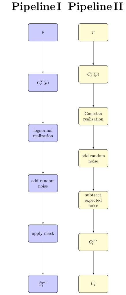
Figure 1: A schematic of the two forward model pipelines used in this work given model parameters $p$. In Pipeline I we develop a forward model of cosmic shear data for inference with DELFI which takes advantage of the forward model approach. There is no need to deconvolve the mask or pixel window function, for example. In Pipeline II we use a Gaussian field, do not use a mask, subtract off the shot-noise or deconvolve the pixel window function. These choices allow us to make a direct comparison between DELFI and a Gaussian likelihood analysis to test the Gaussian likelihood assumption.

II Cosmic Shear Formalism and the Lognormal Field Approximation

II.1 The Lensing Spectrum

Assuming the Limber LoVerde and Afshordi (2008); Kitching et al. (2016), spatially-flat Universe Taylor et al. (2018a), flat sky Kitching et al. (2016) and equal-time correlator approximations Kitching and Heavens (2017), the lensing spectrum, $C_{\ell,\rm GG}^{ij}$, is given by Heymans et al. (2013):

$$C_{\ell,\rm GG}^{ij}=\int_{0}^{r_{\rm H}}dr\,\frac{q_{i}(r)q_{j}(r)}{r^{2}}\,P\left(\frac{\ell}{r},r\right),$$ (1)

where $P(k,r)$ is the matter power spectrum and the lensing efficiency kernel, $q_{i}$ is defined as:

$$q_{i}(r)=\frac{3H_{0}^{2}\Omega_{\rm m}}{2c^{2}}\frac{r}{a(r)}\int_{r}^{r_{\rm H}}\,dr^{\prime}\ n_{i}(r^{\prime})\frac{r^{\prime}-r}{r^{\prime}},$$ (2)

and we generate the $N_{\text{tomo}}$ tomographic bins, $n_{i}(r^{\prime})$, by dividing the radial distribution function:

$$n\left(z_{p}\right)\propto\frac{a_{1}}{c_{1}}{\rm e}^{-\frac{\left(z-0.7\right)^{2}}{b_{1}^{2}}}+{\rm e}^{-\frac{\left(z-1.2\right)^{2}}{d_{1}^{2}}},$$ (3)

with $\left(a_{1}/c_{1},b_{1},d_{1}\right)=\left(1.5/0.2,0.32,0.46\right)$ Van Waerbeke et al. (2013) into bins with an equal number of galaxies per bin. To account for photometric redshift error, each bin is smoothed by the Gaussian kernel:

$$p\left(z|z_{p}\right)\equiv\frac{1}{2\pi\sigma_{z}\left(z_{p}\right)}{\rm e}^{-\frac{\left(z-c_{\rm cal}z_{p}+z_{\rm bias}\right)^{2}}{2\sigma_{z_{p}}}},$$ (4)

with $c_{\rm cal}=1$, $z_{\rm bias}=0$ and $\sigma_{z_{p}}=A\left(1+z_{p}\right)$ with $A=0.05$ Ilbert et al. (2006).

II.2 Intrinsic Alignments

The tidal alignment of galaxies around massive halos adds two additional terms to the lensing spectrum. An ‘II term’ accounts for the intrinsic tidal alignment of galaxies around massive dark matter halos, while a ‘GI term’ accounts for the anti-correlation between tidally aligned galaxies at low redshifts and weakly lensed galaxies at high redshift.

We model this effect using the non-linear alignment (NLA) model Hirata and Seljak (2004); Heymans et al. (2013). We also allow the intrinsic amplitude, $A(z)$, to vary as a function of redshift so that $A(z)=\left[(1+z_{0})/(1+z)\right]^{\eta}$ MacCrann et al. (2015), where $z_{0}$ is the mean redshift of the survey. This is $z_{0}=0.76$ for the $n(z)$ given in equation (3). This model was used in the joint KiDS-450+2dFLenS Joudaki et al. (2017) analysis and was one of the models considered in the Dark Energy Survey Year 1 cosmic shear analysis (hereafter DESY1) Troxel et al. (2017).

In this case the II spectrum, $C_{\ell,\rm II}^{ij}$, is given by:

$$C_{\ell,\rm II}^{ij}=\int_{0}^{r_{\rm H}}dr\,\frac{n_{i}(r)n_{j}(r)}{r^{2}}\,P_{\rm II}\left(\frac{\ell}{r},r\right),$$ (5)

where the II matter power spectrum is:

$$P_{\rm II}(k,z)=F^{2}(z)P(k,z)$$ (6)

and

$$F(z)=-A_{I}C_{1}\rho_{\rm crit}\frac{\Omega_{\rm m}}{D(z)}\left(\frac{1+z\left(r\right)}{1+z_{0}}\right)^{\eta},$$ (7)

where $\rho_{\rm crit}$ is the critical density of the Universe, $D(z)$ is the growth factor and $C_{1}=5\times 10^{-14}h^{-2}M_{\odot}^{-1}{\rm Mpc}^{3}$.

The GI power spectrum is:

$$C_{\ell,\rm GI}^{ij}=\int_{0}^{r_{\rm H}}dr\,\frac{q_{i}(r)n_{j}(r)+n_{i}(r)q_{j}(r)}{r^{2}}\,P_{\rm GI}\left(\frac{\ell}{r},r\right),$$ (8)

and the GI matter power spectrum is:

$$P_{\rm GI}(k,z)=F(z)P(k,z).$$ (9)

Altogether the theoretical lensing spectrum, $C^{T,ij}_{\ell}$, is given by the sum of the three contributions:

$$C^{T}_{\ell}=C_{\ell,\rm GG}^{ij}+C_{\ell,\rm GI}^{ij}+C_{\ell,\rm II}^{ij}$$ (10)

Henceforth we will routinely drop the tomographic bin labels for convenience, as we have done here, on the left hand side.

All lensing spectra are generated inside the Cosmosis framework Zuntz et al. (2015). The linear power spectrum and expansion history are computed with CAMB Lewis and Challinor (2011) and the nonlinear corrections are computed with HALOFIT Takahashi et al. (2012).

II.3 The Lognormal Field Approximation

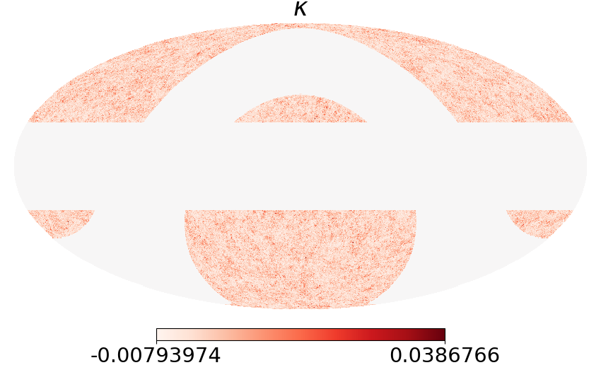
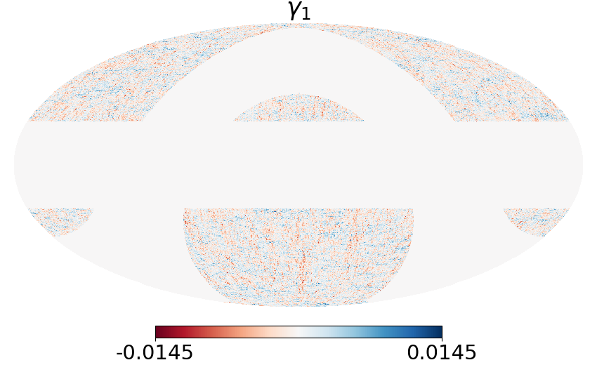
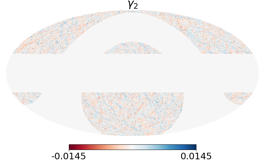
Figure 2: A single masked data realization of the convergence field, $\kappa$, and the two observable shear components: $\gamma_{1}$ and $\gamma_{2}$ (including shape noise) for a typical Stage IV experiment. This is the lowest redshift bin of six, where the effect of non-Gaussianity is largest. The non-Gaussianity is clearly visible in the $\kappa$-map (the color scale runs between the minimum and maximum value of the $\kappa$-field to make the non-Gaussianity more visible), where the majority of pixels are very slightly negative with a small number of pixels taking very large (positive) $\kappa$-values. The mask cuts all pixels lying within $22.5\text{ deg}$ of the galactic and ecliptic planes.

Generating lognormal convergence fields Hilbert et al. (2011) is computationally inexpensive and captures the impact of nonlinear structure growth more accurately than Gaussian realizations. This approximation was recently used in DESY1 Troxel et al. (2017) to compute the covariance matrix from noisy realisations of the data. No differences in parameter constraints were found when the covariance was computed using lognormal fields compared to the halo model approach Krause and Eifler (2017).

In the lognormal field approximation the convergence, $\kappa^{i}(\theta)$, inside each tomographic bin, $i$, is generated by exponentiating and shifting a Gaussian realization, $g^{i}\left(\theta\right)$, according to:

$$\kappa^{i}(\theta)=\text{exp}\left[g^{i}\left(\theta\right)\right]-\kappa^{i}_{0},$$ (11)

where $\kappa^{i}_{0}$ is a constant shift parameter.

We use Flask Xavier et al. (2016) to generate consistent lognormal realizations Hilbert et al. (2011) of the convergence and shear fields – correlated between redshift slices. The procedure is discussed in detail in Section 5.2 of Xavier et al. (2016) (see also Mancini et al. (2018)).

Flask takes just two inputs:

• Flask takes the theoretical lensing spectrum, $C^{T}_{\ell}$, defined in Sections II.1-II.2. Formally Flask uses the convergence spectrum to generate a convergence field, $\kappa$, from which it computes a consistent shear field, $\gamma$. In the flat sky approximation – which we assume throughout – the shear and convergence spectrum are the same, but care would be needed to correctly re-scale the input convergence spectrum by the appropriate $\ell$-factor if the flat sky approximation was dropped Kitching et al. (2016); Castro et al. (2005).

• Flask requires the shift parameter, $\kappa^{i}_{0}$ for each tomographic bin $i$. We compute this by taking a weighted average of the shift parameter at each redshift:

  $$\kappa^{i}_{0}=\int\text{d}z\text{ }n_{i}(z)\kappa^{i}_{0}(z),$$ (12)

  using the fitting formula:

  $$\kappa^{i}_{0}(z)=0.008z+0.029z^{2}-0.0079z^{3}+0.0065z^{4}$$ (13)

  derived from simulations Hilbert et al. (2011).

While the fitting formula will have some cosmological dependence, the shift parameter does not affect the power spectrum of the field – only impacting cosmological constraints through the covariance. Non-Gaussian corrections to the covariance already have a sub-dominant impact Sato and Nishimichi (2013); Eifler et al. (2014), hence the dependence of these corrections on the cosmology is further sub-dominant. For this reason we ignore the cosmological dependence of the shift parameter.

A valid covariance matrix between data must be positive-definite, but this is not guaranteed for correlations between tomographic lognormal fields Xavier et al. (2016). Flask overcomes this issue by perturbing the lognormal fields following the regularization procedure outlined in Section 3.1 of Xavier et al. (2016). Provided that the regularization is applied to a small number of tomographic bins, it is found in Xavier et al. (2016) that $C_{\ell}^{\text{reg}}/C_{\ell}^{{\rm ln}}\ll 1\times 10^{-5}$, where $C_{\ell}^{\text{reg}}$ is the recovered regularized spectrum and $C_{\ell}^{{\rm ln}}$ is the spectrum recovered from the unregularized map Xavier et al. (2016). In Section V we verify that this will not impact Stage III parameter constraints.

In Figure 2 we plot a single lognormal realization generated with Pipeline I. We show the masked convergence and components of the shear field in the lowest redshift bin. This is where the non-Gaussianities are most pronounced and clearly visible. In the convergence map the majority of the pixels take small negative values. However there are rare incidences of large positive convergence. This physically corresponds to collapsed high-density structures along the line-of-sight.

II.4 Band-limit Bias from the Lognormal Field

Unlike Gaussian fields, lognormal realizations are not band-limited in $\ell$ Xavier et al. (2016) (see Section 5.2.2 therein). In particular, Taylor expanding the lognormal convergence field, $\kappa^{i}(\theta)$, in terms of the Gaussian field, $g^{i}\left(\theta\right)$, yields quadratic and higher order terms in $g^{i}$. In harmonic space this mixes different $\ell$-modes. When a band-limit is imposed, this biases the lensing spectrum recovered from the map.

III Cosmological Parameter Inference

III.1 Gaussian likelihood Analysis

In the standard two-point cosmic shear likelihood analysis, we assume a Gaussian likelihood:

$$\text{ln }\mathcal{L}\left(p\right)=-\frac{1}{2}\sum_{a,b}\left[D_{a}-T_{a}\left(p\right)\right]C_{ab}^{-1}\left[D_{b}-T_{b}\left(p\right)\right],$$ (14)

where $D_{a}$ and $T_{a}\left(p\right)$ are the data and theory vectors respectively composed of the $C_{\ell}$ estimated from data and the theoretical expectation of $C_{\ell}$ given cosmological parameters $p$.

Meanwhile $C_{ab}^{-1}$ is the inverse of the covariance matrix. Since we generate the covariance matrix from noisy simulations of the data we make the Anderson-Hartlap Hartlap et al. (2007); Anderson et al. (1958) correction, to avoid bias from inverting the covariance matrix, for the remainder of the paper.

III.2 The Potential Insufficiency of the Gaussian likelihood Approximation in Cosmic Shear

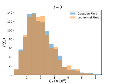
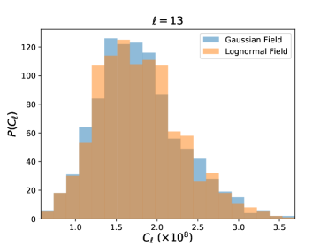
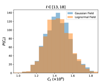
Figure 3: The distribution of $C_{\ell}$ drawn from 1000 Gaussian (blue) and lognormal (orange) realizations. Each subplot corresponds to different $\ell$-mode and binning strategy. In all cases there is little difference in the skew of the distribution when using Gaussian or lognormal fields. This suggests the impact of the Gaussian likelihood approximation can be tested under the assumption of a Gaussian field, as in this work. Top: The $\ell=3$ case is clearly skewed, as expected for low-$\ell$ (see Section III.2). Middle: The $\ell=13$ case is slightly less skewed, as expected. Bottom: The binned case for $\ell\in[13,15]$. By the central limit theorem, the distribution is Gaussianized when drawing randomly from the distribution of each independent $\ell$-mode.

To see why the Gaussian likelihood assumptions can lead to bias we summarize the argument given in Sellentin et al. (2018). Inside a single bin the unmasked lensing spectrum is:

$$C_{\ell}=\frac{1}{2\ell+1}\sum_{m=-\ell}^{\ell}\mid\gamma_{\ell m}\mid^{2}.$$ (15)

Since the harmonic coefficients, $\gamma_{\ell m}$, are computed as a summation over a large number of pixels, they are Gaussian distributed by the central limit theorem. Squaring a Gaussian random variable gives a gamma distribution – which is left-skewed. This is illustrated in the top two rows of Figure 3.

Taking a Gaussian rather than a gamma distribution for the likelihood could bias parameter constraints. Since $S_{8}^{2}=\sigma_{8}^{2}(\Omega_{m}/0.3)$ and $\Omega_{m}$ enter into the shear spectrum amplitude, we would expect these parameters to be ones which are most affected – and biased low. Only in the limit of large $\ell$ – as the $C_{\ell}$ itself becomes the sum over a large number of $m$-modes – does the central limit theorem kick in and the likelihood become Gaussian. This is illustrated in Figure 3 and can be seen by comparing the second and third row.

III.3 Density-estimation Likelihood-free Compression

Since density-estimation likelihood-free inference methods are most effective in low dimensions Alsing et al. (2018), we compress the $C_{\ell}$ summary statistic. As suggested in Alsing and Wandelt (2018), the lensing spectra are compressed into a new vector, $t$, according to:

$$C_{\ell}\rightarrow t=\nabla_{p}\mathcal{L}_{\ast},$$ (16)

where $p$ is the set of cosmological parameters that we are inferring, $\mathcal{L}_{\ast}$ is a proposal Gaussian likelihood centred at a fiducial set of parameters which we take to be $\left(\Omega_{m},h_{0},\Omega_{b},n_{s},S_{8},A,\eta\right)=\left(0.3,0.72,0.96,0.79,1.,2.8\right)$ throughout, where $S_{8}=\sigma_{8}(\Omega_{m}/0.3)^{0.5}$, $A$ and $\eta$ are the intrinsic alignment parameters defined in Section II.2 and the other parameters take their standard cosmological definitions. As the assumption of a Gaussian likelihood here is only for compression purposes, it does not bias the final parameter constraints and the Fisher information is preserved provided the true likelihood is Gaussian Alsing and Wandelt (2018). If the true likelihood is not exactly Gaussian, some information will be lost. This is investigated in Section VI. For more advanced compression techniques using neural networks, see Charnock et al. (2018).

III.4 Density-estimation Likelihood-free Inference

We use pydelfi Justin Alsing (2019) to learn the conditional density $\mathbb{P}(t|p)$ (this software comes with many different run-mode options, but we restrict our attention to the methods used in this work). The likelihood is then given by $\mathbb{P}(t=t_{\text{data}}|p)$, where $t_{\text{data}}$ is the mock data generated from either Pipeline I or II. Multiplying by the prior, which we take to be flat in all parameters, yields the posterior.

Using the default setting in pydelfi, we train five neural density estimators (NDE) (four mixture density networks (MDN) and one masked autoregressive flow (MAF), see Justin Alsing (2019) for more details) with the default network architectures described in Section 4 of Justin Alsing (2019), parameterized in terms of a set of neural network weights, $w$. Training multiple networks allows DELFI to avoid over-fitting and increases robustness.

We use sequential learning to learn the weights, $w$, updating our knowledge of the conditional density distribution $\mathbb{P}(t=t_{\text{data}}|p)$. Specifically we divide the inference task into 20 training steps with 100 simulations per step. Given a large enough computer all the simulations in each training step could be run in parallel, so that the total time of the simulations would not exceed the time it took to perform 20 simulations.

As an initial guess for the conditional distribution, we take the multivariate Gaussian:

$$\mathbb{P}(t|p)=\mathcal{N}(t|p,F^{-1}),$$ (17)

where $F^{-1}$ is the inverse of the Fisher matrix of the cosmological parameters, $F=-\langle\nabla_{p}\nabla_{p}^{Tr}\mathcal{L}_{*}\rangle$. At each step thereafter, we train each neural density estimator on a set of parameter realization pairs $\{p_{i},t_{i}\}$ drawing samples from the conditional density of the previous step to ensure that the highest density regions are the most finely sampled. Meanwhile ten percent of the samples are retained as a validation set to avoid over-fitting.

At each step each NDE learns the weights, $w$, by minimizing the negative loss function:

$$-\ln U(w)=-\sum_{i=1}^{N_{\text{samples}}}\ln\mathbb{P}(t_{i}|p,w),$$ (18)

which is an estimate of the Kullback-Leibler divergence between the density estimator $\mathbb{P}(t=t_{\text{data}}|p)$ and the true distribution Justin Alsing (2019) (the minus sign is pulled out of $U(w)$ on the left-hand side following the convention in Justin Alsing (2019)). The final estimate for the conditional distribution is given as a weighted average over the estimates from the five networks:

$$\mathbb{P}(t|p;w)=\sum_{i\in\text{networks}}\beta_{i}\mathbb{P}_{i}(t|p;w),$$ (19)

where the weights are determined by the relative likelihood of each NDE Justin Alsing (2019).

IV The Full Forward Model

In this section we use Pipeline I to generate mock Stage IV data and then run analysis DA1 to recover the input cosmology. This allows us to test our pipeline and estimate the number of simulations needed for a Stage IV experiment. We describe the model choices and results below.

IV.1 The Mask

We use a typical Stage IV survey mask shown in Figure 2. All pixels lying within $22$ deg of either the galactic or ecliptic planes are masked. This leaves 14,490 $\text{deg}^{2}$ of unmasked pixels which, as a fraction of the full sky, is $f_{\text{sky}}=0.35$.

IV.2 Shot-Noise Model

The noise, $\gamma_{p}$, for each pixel, $p$, is drawn from a Gaussian distribution Alsing et al. (2015a):

$$\gamma_{p}\sim\mathcal{N}\left(0,\frac{\sigma_{\epsilon}}{\sqrt{\widehat{N}_{P}}}\right)$$ (20)

where $\widehat{N}_{P}$ is the number of galaxies in each pixel, the orientation is angle is drawn from a uniform distribution, we take the intrinsic shape dispersion as $\sigma_{\epsilon}=0.3$ Brown et al. (2002) and use $30\text{ galaxies per arcmin}^{2}$ throughout. This is a good approximation since in all our simulations there are a large number of galaxies in each pixel, so the central limit theorem applies.

IV.3 Forward Modelling the Mask

One advantage of performing inference with full forward models of the data is that we do not need to deconvolve the mask. This is both computationally simpler and avoids the risk of bias from inaccurate deconvolution which is present in the standard likelihood analysis.

Given two masked shear fields $a(\theta)$ and $b(\theta)$, a naïve estimate of the lensing spectrum is the pixel pseudo-$C_{\ell}$ spectrum:

$$\widetilde{C}^{\text{pix},EE}_{\ell}=\frac{1}{2\ell+1}\sum_{m=-\ell}^{\ell}\langle a^{E}_{lm}b^{E}_{lm}\rangle,$$ (21)

where the tilde is used to denote the fact that we have not corrected for the mask and the ‘pix’ superscript reminds us that we have not accounted for the pixel window function. Analogous expressions are easily found for the $EB$ and $BB$ spectra.

In an unmasked field, lensing by large scale structure will only induce power in the $EE$ spectra, but to retain information leaked into the $EB$ and $BB$ spectra due to the presence of a mask, in Pipeline I, we use:

$$\widetilde{C}_{\ell}^{\text{pix}}=\widetilde{C}_{\ell}^{\text{pix},EE}+\widetilde{C}_{\ell}^{\text{pix},EB}+\widetilde{C}_{\ell}^{\text{pix},BE}+\widetilde{C}_{\ell}^{\text{pix},BB},$$ (22)

as the estimator. This is computed using HEALpy Gorski et al. (1999); Górski et al. (2005).

In a future pipeline it may still be desirable to use the pseudo-$C_{\ell}$ formalism to avoid mixing between $E$ and $B$-modes, allowing us to immediately remove $B$-modes induced by unknown systematics. As long as the data and theory are treated in the same way the pseudo-$C_{\ell}$ formalism will not introduce bias, as it could in the standard likelihood analysis.

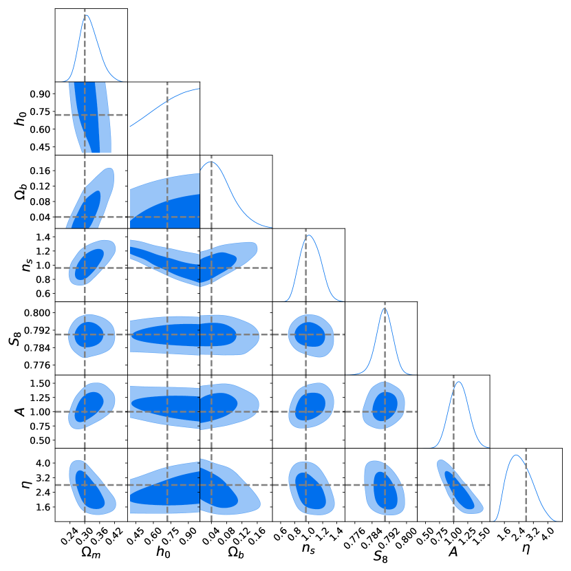
Figure 4: $68\%$ and $95\%$ credible region parameter constraints found with DELFI analysis DA1 after 1000 simulations, for a mock Stage IV experiment. We confirm that we recover the input cosmology within statistical errors. We plot the convergence in Figure 5. In a realistic situation there may be a larger number of nuisance parameters. This would not dramatically slow convergence because we could ‘nuisance harden’ the data compression step, to only learn the posterior for the parameters of interest Alsing and Wandelt (2019).

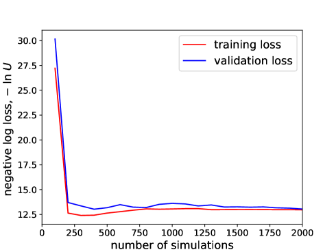
Figure 5: The negative loss function defined in equation (18) for the training and validation sets as a function of the number of simulations. This suggests that $\mathcal{O}(1000)$ simulations are needed for a Stage IV experiment. This is similar to the number found in Justin Alsing (2019), which only considered a simple Gaussian field forward model with no intrinsic alignments, implying that the convergence rate is fairly insensitive to the precise details of the model.

IV.4 Mimicking a Stage IV Experiment

To estimate the number of simulations needed for a Stage IV experiment and ensure that pipeline recovers the input cosmology we produce mock data with Pipeline I. We use 6 tomographic bins sampling 15 logarithmically spaced $\ell$-bins in the range $\ell\in[10,1000].$ We then run pydelfi to estimate the posterior distribution of the cosmological parameters for this data. The final parameter constraints for a lambda cold dark matter (LCDM) cosmology with two nuisance intrinsic alignment parameters are shown in Figure 4. This confirms that we recover the input parameters within errors.

In Figure 5 we plot the negative loss function defined in equation (18) for the training and validation sets. Both have converged within $\mathcal{O}(1000)$ simulations. This is similar to the number found in the simple Gaussian field pipeline presented in Justin Alsing (2019), suggesting that the inclusion of higher order effects including intrinsic alignments and non-Gaussian field corrections does not significantly increase the required number of simulations.

When working with real data, we may require a large number of nuisance parameters. Nevertheless, we do not expect this to dramatically increase the number of simulations needed, since we can always tune the data compression to maximize the information retention of the parameters of interest, following the procedure in Alsing and Wandelt (2019).

Each simulation takes approximately 33 minutes on a single thread of a 1.8 GHz Intel Xeon (E5-2650Lv3) Processor. Thus if run on 100 threads in parallel, the total simulation time of the DELFI inference step takes only 10 hours. Many of the individual modules in the pipeline are multithreaded (e.g Flask), so running on even more threads would further reduce the total run-time.

V Prospects for Stage III Data

In this section we discuss the viability of applying analysis DA1 to existing Stage III data. For the remainder of this section we assume a circular mask of $4951\text{ deg}^{2}$, similar to the final coverage of the Dark Energy Survey Troxel and Ishak (2015) with $10{\rm\ galaxies\ per\ arcmin}^{2}$ and use Pipeline I throughout this section – except where modifications are explicitly stated.

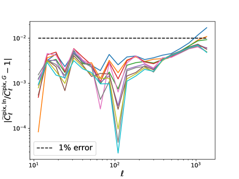
Figure 6: The colored lines show the absolute value of the difference between the average recovered cross and intra-bin spectra from 100 lognormal and 100 Gaussian realizations ($4$ tomographic bins, $N_{\text{side}}=512$ and $\ell\in[10,1535]$). The difference is due to the band-limit bias in the lognormal field discussed in Section II.4. With these model choices the band-limit bias is safely below $1\%$ for nearly all data points.

V.1 Validating the Lognormal Simulations

Lognormal fields were used to generate the covariance matrix in the recent Dark Energy Survey Year 1 analysis Troxel et al. (2017). The authors found no difference in parameter constraints between this analysis and one which used a halo model to generate the covariance matrix – but to verify that our pipeline is ready for Stage III data, we must also ensure that we recover an unbiased $C_{\ell}$ from the maps.

Given an accurate input $C_{\ell}$, the only bias in Pipeline I comes from regularizing the map (see Section II.3). We would not expect the band-limit bias of the lognormal field to be problematic since imposing a band-limit would affect the data in the same way. However this assumes that the true field is exactly lognormal. Nevertheless we check to ensure that the combined effect of regularization and imposing a band-limit is small. We quantify this statement by finding the difference between the average recovered pixelated $C_{\ell}$’s from 100 Gaussian simulations (where no band-limit bias or regularization bias is present) and 100 lognormal simulations. Each $4$-tomographic bin simulation takes approximately 15 minutes on a single thread and the difference in the recovered spectra is shown in Figure 6. The bias is safely below $1\%$ in all but three data points. This confirms that once minor updates have been made (see next subsection), the pipeline will be ready for use on today’s data.

V.2 Model Improvements

Only a small number of adjustments must be made to DA1 to apply this analysis to existing data. These are:

• We must accurately account for baryonic physics. This can be handled using a halo model code Mead et al. (2015), potentially in combination with the k-cut cosmic shear approach Taylor et al. (2018b); Bernardeau et al. (2014), optimally cutting scales which can not be accurately modeled.

• We must introduce several nuisance parameters. As well as allowing for free multiplicative and additive shear biases, photo-z bias parameters will need to be allowed to vary, as in the Dark Energy Year 1 analysis Troxel et al. (2017). This will increase the number of nuisance parameters. To avoid excessive computational costs we must ‘nuisance harden’ Alsing and Wandelt (2019) the data compression step.

VI Testing the Gaussian Likelihood Approximation

In this section we compare DELFI and the standard Gaussian likelihood analysis by running the DA2 analysis and the LA analysis, on the same mock Stage IV data. We use Pipeline II to generate the mock data, produce the covariance matrix and generate the forward models in DA2. Since DELFI does not assume any particular likelihood, differences in the resulting parameter constraints are only due to the Gaussian likelihood assumption in LA. Because we can not just forward model everything in LA, care must be taken to ensure that the band-limit bias, deconvolving the mask, deconvolving the pixel window function and subtracting the shot-noise does not lead to additional bias between the two analyses. Controlling for these effects is described in the first subsection.

VI.1 Modeling Choices In Pipeline II

To avoid the band-limit bias we use a Gaussian field, rather than the lognormal field.

We do not apply a mask in DA2 as we have found that using the pseudo-$C_{\ell}$ method

(with the public code NaMaster Alonso et al. (2018)) can bias parameter constraints, with our choice of HEALpix  $N_{\rm side}$ and $\ell_{\rm max}$ by up to $1\sigma$. Instead we adjust the galaxy number density so that total number of galaxies and hence the signal-to-noise remains unchanged.

In LA we decide to take the $C_{\ell}$, with no shot-noise term in the intra-bin case, as the data vector. Thus we must subtract off the expected value of the noise in DA2. This is computed by running 500 noise-only simulations, as in the analysis of Hikage et al. (2018).

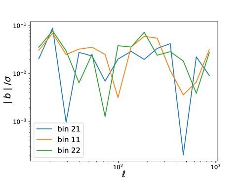
Figure 7: The absolute value of the bias, $\mid b\mid$, due to imperfect pixel-window deconvolution and noise subtraction relative to the statistical error, $\sigma$, from 500 Pipeline II simulations. This confirms that the comparison between DELFI and the likelihood analysis presented in Section VI.2 will be unaffected.

We must also account for the fact that the shear spectra are computed on pixelized maps – that is, we must deconvolve the pixel window function, $w_{\ell}$, which is defined in Jeong et al. (2014) and computed using HEALpix. This assumes that the scale of the signal is large relative to the pixel scale and that all pixels are the same shape. The window-corrected spectrum, $C_{\ell}$, is given in terms of the spectrum computed from a pixelized map, $C_{\ell}^{\text{p}ix}$, by:

$$C_{\ell}=w_{\ell}^{-2}C_{\ell}^{\text{p}ix}.$$ (23)

By running 500 Gaussian field simulations we have confirmed that the combined bias from deconvolving the pixel window function and subtracting the shot-noise is small, so that we can fair comparison between the DA2 analysis and the LA analysis. This is shown in Figure 7. The absolute value of the bias, $|b|$, is small relative to the statistical error, $\sigma$, with $|b|/\sigma<0.1$ for all data points.

VI.2 Impact of the Gaussian Likelihood Approximation

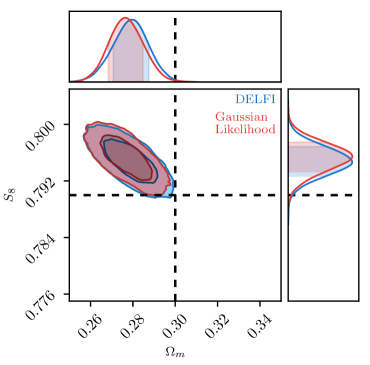
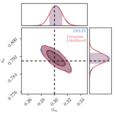
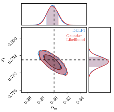
Figure 8: The $68\%$ and $95\%$ credible region parameter constraints for three random data realizations found using a MCMC Gaussian likelihood analysis and DELFI, which makes no assumption about the functional form of the likelihood. The mock data input cosmology is labeled by black dotted lines. Only in the first realization, does the input cosmology lie outside the $68\%$ credible region – but statistically this is to be expected for a small number of realizations. The contours found using the two different analyses are very similar for all three data realizations suggesting that the Gaussian likelihood approximation has negligible impact, and the compression in equation (16) is lossless. This former statement is confirmed in Figure 9.

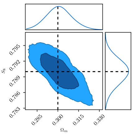
Figure 9: The $68\%$ and $95\%$ credible region of the MLE distribution, assuming a Gaussian likelihood. The value of the input cosmology is indicated by the black dotted lines, and lies at the center of the contours. This implies that the Gaussian likelihood approximation does not lead to any measurable bias in our setup.

To test the impact of the Gaussian likelihood approximation we first generate 1000 mock data realizations using Pipeline II. We take 15 logarithmically spaced $\ell$-bins in the range $[10,1000]$ and restrict our attention to the $S_{8}-\Omega_{m}$ plane. To cut computation cost, we use only two tomographic bins. The parameters $S_{8}$ and $\Omega_{m}$ primarily impact the amplitude of the shear spectrum, so we do not expect to lose too much information with this choice Taylor et al. (2019); Spurio Mancini et al. (2018).

It is known from analyses of cosmic microwave background temperature anisotropies that non-Gaussian likelihoods arise even for Gaussian fields Hamimeche and Lewis (2008), as the argument given in Section III.2 holds for any field configuration. Nevertheless we generate $1000$ lognormal realizations in conjunction with the Gaussian fields to determine whether the field configuration impacts the likelihood. The results are plotted in Figure 3. The skew in the likelihood is indistinguishable between the Gaussian and lognormal field configurations, justifying our choice to work with Gaussian fields for the remainder of this section.

For three random data realizations, we run a DELFI and a Gaussian likelihood analysis. The resulting posteriors are shown in Figure 8. Each subplot corresponds to one of the three realizations.

In all three cases the DELFI and Gaussian likelihood contours are very similar. This suggests the Gaussian likelihood assumption does not bias parameter constraints in the $S_{8}-\Omega_{m}$ plane and the compression defined in equation (16) is lossless.

To confirm and quantify this statement, we sample the maximum likelihood estimator (MLE) distribution assuming a Gaussian likelihood, using the 1000 data realizations generated earlier. For each realization, the MLE is found using the Nelder-Mead algorithm built into scipy and wrapped into Cosmosis using the default settings. The resulting MLE distribution is shown in Figure 9. The input cosmology lies almost exactly at the center of the $68\%$ credible region which implies that there is no measurable bias from the Gaussian likelihood approximation.

We stress that these conclusions only hold for the $C_{\ell}$ analysis presented in this work. In particular, the $\ell$-binning strategy matters. By binning $\ell$-modes we are taking a sum over random variables, so by the central limit theorem broader bins correspond to more Gaussian data. This is verified in Figure 3 and can be seen by comparing the skew in the second and third row. The Gaussian likelihood approximation could be important for much narrower bins. While the Gaussian likelihood approximation may not be valid for other weak lensing summary statistics, a recent paper has shown it is also valid for two-point correlation functions Lin et al. (2019).

VII Future Prospects

We review the main known cosmic shear systematics which must eventually be included in the full forward model. To account for many of these effects we must first take the base model presented in this work to ‘catalog level’. This can be done by first generating a consistent density field – either with Flask or by taking the difference between two neighbouring tomographic bins – and then populating the density field with a realistic population of galaxies Miller et al. (2007) assuming a biased tracer model (e.g Elvin-Poole et al. (2018)). Cosmic shear systematics break down into four broad categories: data-processing, theoretical, astrophysical and instrumental systematics.

On the data-processing side, accurately measuring the shape and photometric redshift of galaxies is the primary challenge. Both measurements are dependent on the galaxy-type Kannawadi et al. (2018), and this is in turn correlated with the density through the morphology-density relation Houghton (2015). Rather than using the best fit parameters for each galaxy, we can sample the posterior on each galaxy as in a Bayesian hierarchical model Alsing et al. (2015a) to propagate the measurement uncertainty into the final parameter constraints, as suggested in Justin Alsing (2019). We can also account for image blending Kannawadi et al. (2018); Samuroff et al. (2017) more easily with forward models.

Two important theoretical systematics are the reduced shear correction Dodelson et al. (2006); Bartelmann and Schneider (2001) and magnification bias Hamana (2001); Liu et al. (2014). The former correction accounts for the fact that we measure the reduced shear $\gamma/(1-\kappa)$ with a weak lensing experiment. In a likelihood analysis, this can be computed using a perturbative expansion as in  Dodelson et al. (2006); Shapiro (2009). This is slow and requires us to rely on potentially inaccurate fitting functions for the lensing bispectrum. Meanwhile the magnification bias accounts for the fact that galaxies of the same luminosity can fall above (below) the detectability limit in regions of high (low) lensing magnification. In both cases, these systematics can be easily handled with full forward models of consistent shear and convergence fields.

The two dominant instrumental systematics are the telescope’s point spread function (PSF) Massey et al. (2012) and the effect of charge transfer inefficiency (CTI) in the charge-coupled devices (CCDs) Massey et al. (2012); Rhodes et al. (2010). Efforts are underway to build pipelines which characterize these effects in upcoming experiments (e.g Vavrek et al. (2016) and Paykari et al. (in prep)). Integrating these pipelines into ours would enable the propagation of instrumental errors through to the final parameter constraints.

On the astrophysical side, the two dominant systematics are the impact of baryons on the density field Semboloni et al. (2010) and the intrinsic alignment of galaxies Hirata and Seljak (2004); Kiessling et al. (2015). For Stage IV data, forward models will likely have to be based on high-resolution N-body lensing simulations Izard et al. (2017); Kiessling et al. (2011) to include the effects of baryons. Even with today’s highest resolution simulations the impact baryons is still uncertain Huang et al. (2018), so it will likely be necessary to optimally cut Taylor et al. (2018b) or marginalize out uncertain scales Huang et al. (2018). Meanwhile more sophisticated intrinsic alignment models which account for different alignment behaviour by galaxy type Samuroff et al. (2018) will need to be included.

Eventually higher-order statistics such as peak counts and the shear bispectrum can be added. Since DELFI automatically handles multiple summary statistics in a unified way, the constraints will be tighter than doing the two-point and higher-order statistic analyses separately. With a greater ability to handle systematics, DELFI may also open up the possibility of performing inference with weak lensing flux and size magnification Justin Alsing (2019); Alsing et al. (2015b); Duncan et al. (2013); Huff and Graves (2013); Hildebrandt et al. (2013); Heavens et al. (2013).

VIII Conclusion

By comparing a Gaussian likelihood analysis to a fully likelihood-free DELFI analysis, we have found that the Gaussian likelihood approximation will have a negligible impact on Stage IV parameters constraints. Nevertheless we recommend the development of DELFI weak lensing pipelines, because they offer the possibility of performing rapid parallel inference on full forward realizations of the shear data. In the future, this will allow us to seamlessly handle astrophysical and detector systematics – at a minimal computational cost. Since we have shown that applying the standard DELFI data compression (see equation 16) to the $C_{\ell}$ summary statistic is lossless (see Figure 8), this comes at no cost in terms of constraining power.

We have taken the first steps towards developing a pipeline to rapidly generate realistic non-Gaussian shear data, including the impact of intrinsic alignments. These effects are handled in the same way as the Dark Energy Survey year 1 analysis Troxel et al. (2017) and we have verified that the regularisation of the lognormal field will not lead to bias using today’s data. Additionally the pipeline is computationally inexpensive, so in the future it will be useful for quickly determining which systematics are important.

We confirm the result of Justin Alsing (2019) (which used a simple Gaussian field model for lensing field) that $\mathcal{O}(1000)$ would be required to perform inference on Stage IV data. This suggests that this estimate is robust and largely insensitive precise details of the cosmic shear forward model.

We conclude that DELFI has a promising future in cosmic shear studies. Developing fast simulations that fully integrate all relevant astrophysical, detector and modelling effects is the primary hurdle. With so many clear advantages over the traditional likelihood analysis, developing these simulations should be a priority.

IX Acknowledgements

PLT thanks Luke Pratley, David Alonso and Martin Kilbinger. BDW thanks Chris Hirata for asking him a question a decade ago that is answered in this paper. The authors would like to thank the referee whose comments have helped significantly improve the clarity of this paper. We are indebted to the developers of all public code used in this work. PLT acknowledges the hospitality of the Flatiron Institute.

This work was supported by a collaborative visit funded by the Cosmology and Astroparticle Student and Postdoc Exchange Network (CASPEN). PLT is supported by the UK Science and Technology Facilities Council. TDK is supported by a Royal Society University Research Fellowship. JA was partially supported by the research project grant “Fundamental Physics from Cosmological Surveys” funded by the Swedish Research Council (VR) under Dnr 2017- 04212. BDW is supported by the Simons foundation. The authors acknowledge the support of the Leverhulme Trust.

References

- Laureijs et al. (2010) R. J. Laureijs, L. Duvet, I. E. Sanz, P. Gondoin, D. H. Lumb, T. Oosterbroek, and G. S. Criado, in Proc. SPIE, Vol. 7731 (2010) p. 77311H.
- Spergel et al. (2015) D. Spergel, N. Gehrels, C. Baltay, D. Bennett, J. Breckinridge, M. Donahue, A. Dressler, B. Gaudi, T. Greene, O. Guyon, et al., arXiv preprint arXiv:1503.03757 (2015).
- (3) J. Anthony and L. Collaboration, in Proc. of SPIE Vol, Vol. 4836, p. 11.
- Heymans et al. (2013) C. Heymans, E. Grocutt, A. Heavens, M. Kilbinger, T. D. Kitching, F. Simpson, J. Benjamin, T. Erben, H. Hildebrandt, H. Hoekstra, et al., Monthly Notices of the Royal Astronomical Society 432, 2433 (2013).
- Troxel et al. (2017) M. Troxel, N. MacCrann, J. Zuntz, T. Eifler, E. Krause, S. Dodelson, D. Gruen, J. Blazek, O. Friedrich, S. Samuroff, et al., arXiv preprint arXiv:1708.01538 (2017).
- Kitching et al. (2014) T. Kitching, A. Heavens, J. Alsing, T. Erben, C. Heymans, H. Hildebrandt, H. Hoekstra, A. Jaffe, A. Kiessling, Y. Mellier, et al., Monthly Notices of the Royal Astronomical Society 442, 1326 (2014).
- Hildebrandt et al. (2017) H. Hildebrandt, M. Viola, C. Heymans, S. Joudaki, K. Kuijken, C. Blake, T. Erben, B. Joachimi, D. Klaes, L. Miller, et al., Monthly Notices of the Royal Astronomical Society (2017).
- Hikage et al. (2018) C. Hikage, M. Oguri, T. Hamana, S. More, R. Mandelbaum, M. Takada, F. Köhlinger, H. Miyatake, A. J. Nishizawa, H. Aihara, et al., arXiv preprint arXiv:1809.09148 (2018).
- Semboloni et al. (2010) E. Semboloni, T. Schrabback, L. van Waerbeke, S. Vafaei, J. Hartlap, and S. Hilbert, Monthly Notices of the Royal Astronomical Society 410, 143 (2010).
- Fu et al. (2014) L. Fu, M. Kilbinger, T. Erben, C. Heymans, H. Hildebrandt, H. Hoekstra, T. D. Kitching, Y. Mellier, L. Miller, E. Semboloni, et al., Monthly Notices of the Royal Astronomical Society 441, 2725 (2014).
- Peel et al. (2017) A. Peel, C.-A. Lin, F. Lanusse, A. Leonard, J.-L. Starck, and M. Kilbinger, Astronomy & Astrophysics 599, A79 (2017).
- Jain and Van Waerbeke (2000) B. Jain and L. Van Waerbeke, The Astrophysical Journal Letters 530, L1 (2000).
- Gupta et al. (2018) A. Gupta, J. M. Z. Matilla, D. Hsu, and Z. Haiman, Physical Review D 97, 103515 (2018).
- Massey et al. (2012) R. Massey, H. Hoekstra, T. Kitching, J. Rhodes, M. Cropper, J. Amiaux, D. Harvey, Y. Mellier, M. Meneghetti, L. Miller, et al., Monthly Notices of the Royal Astronomical Society 429, 661 (2012).
- Jarvis (2004) M. Jarvis, Mon. Not. R. Astron. Soc. 352, 338 (2004).
- Alsing et al. (2015a) J. Alsing, A. Heavens, A. H. Jaffe, A. Kiessling, B. Wandelt, and T. Hoffmann, Monthly Notices of the Royal Astronomical Society 455, 4452 (2015a).
- Alsing et al. (2016) J. Alsing, A. Heavens, and A. H. Jaffe, Monthly Notices of the Royal Astronomical Society 466, 3272 (2016).
- Dodelson et al. (2006) S. Dodelson, C. Shapiro, and M. White, Physical Review D 73, 023009 (2006).
- Sellentin and Heavens (2017) E. Sellentin and A. F. Heavens, Monthly Notices of the Royal Astronomical Society 473, 2355 (2017).
- Sellentin et al. (2018) E. Sellentin, C. Heymans, and J. Harnois-Déraps, Monthly Notices of the Royal Astronomical Society 477, 4879 (2018).
- Bonassi et al. (2011) F. V. Bonassi, L. You, and M. West, Statistical applications in genetics and molecular biology 10 (2011).
- Papamakarios et al. (2018) G. Papamakarios, D. C. Sterratt, and I. Murray, arXiv preprint arXiv:1805.07226 (2018).
- Fan et al. (2013) Y. Fan, D. J. Nott, and S. A. Sisson, Stat 2, 34 (2013).
- Papamakarios et al. (2016) G. Papamakarios, I. Murray, and T. Pavlakou, “Advances in neural information processing systems,” (2016).
- Alsing et al. (2018) J. Alsing, B. Wandelt, and S. Feeney, Monthly Notices of the Royal Astronomical Society 477, 2874 (2018).
- Lueckmann et al. (2018) J.-M. Lueckmann, G. Bassetto, T. Karaletsos, and J. H. Macke, arXiv preprint arXiv:1805.09294 (2018).
- Justin Alsing (2019) S. F. B. W. Justin Alsing, Tom Charnock, arXiv preprint arXiv:1903:00007 (2019).
- Ishida et al. (2015) E. Ishida, S. Vitenti, M. Penna-Lima, J. Cisewski, R. de Souza, A. Trindade, E. Cameron, V. Busti, C. collaboration, et al., Astronomy and Computing 13, 1 (2015).
- Alsing and Wandelt (2018) J. Alsing and B. Wandelt, Monthly Notices of the Royal Astronomical Society: Letters 476, L60 (2018).
- Leclercq (2018) F. Leclercq, Physical Review D 98, 063511 (2018).
- Leclercq et al. (2019) F. Leclercq, W. Enzi, J. Jasche, and A. Heavens, arXiv preprint arXiv:1902.10149 (2019).
- Alsing and Wandelt (2019) J. Alsing and B. Wandelt, arXiv preprint arXiv:1903:01473 (2019).
- LoVerde and Afshordi (2008) M. LoVerde and N. Afshordi, Physical Review D 78, 123506 (2008).
- Kitching et al. (2016) T. D. Kitching, J. Alsing, A. F. Heavens, R. Jimenez, J. D. McEwen, and L. Verde, arXiv preprint arXiv:1611.04954 (2016).
- Taylor et al. (2018a) P. L. Taylor, T. D. Kitching, J. D. McEwen, and T. Tram, Phys. Rev. D 98, 023522 (2018a).
- Kitching and Heavens (2017) T. D. Kitching and A. Heavens, Physical Review D 95, 063522 (2017).
- Van Waerbeke et al. (2013) L. Van Waerbeke, J. Benjamin, T. Erben, C. Heymans, H. Hildebrandt, H. Hoekstra, T. D. Kitching, Y. Mellier, L. Miller, J. Coupon, et al., Monthly Notices of the Royal Astronomical Society 433, 3373 (2013).
- Ilbert et al. (2006) O. Ilbert, S. Arnouts, H. McCracken, M. Bolzonella, E. Bertin, O. Le Fevre, Y. Mellier, G. Zamorani, R. Pello, A. Iovino, et al., Astronomy & Astrophysics 457, 841 (2006).
- Hirata and Seljak (2004) C. M. Hirata and U. Seljak, Physical Review D 70, 063526 (2004).
- MacCrann et al. (2015) N. MacCrann, J. Zuntz, S. Bridle, B. Jain, and M. R. Becker, Monthly Notices of the Royal Astronomical Society 451, 2877 (2015).
- Joudaki et al. (2017) S. Joudaki, C. Blake, A. Johnson, A. Amon, M. Asgari, A. Choi, T. Erben, K. Glazebrook, J. Harnois-Déraps, C. Heymans, et al., Monthly Notices of the Royal Astronomical Society 474, 4894 (2017).
- Zuntz et al. (2015) J. Zuntz, M. Paterno, E. Jennings, D. Rudd, A. Manzotti, S. Dodelson, S. Bridle, S. Sehrish, and J. Kowalkowski, Astronomy and Computing 12, 45 (2015).
- Lewis and Challinor (2011) A. Lewis and A. Challinor, Astrophysics Source Code Library (2011).
- Takahashi et al. (2012) R. Takahashi, M. Sato, T. Nishimichi, A. Taruya, and M. Oguri, The Astrophysical Journal 761, 152 (2012).
- Hilbert et al. (2011) S. Hilbert, J. Hartlap, and P. Schneider, Astronomy & Astrophysics 536, A85 (2011).
- Krause and Eifler (2017) E. Krause and T. Eifler, Monthly Notices of the Royal Astronomical Society 470, 2100 (2017).
- Xavier et al. (2016) H. S. Xavier, F. B. Abdalla, and B. Joachimi, Monthly Notices of the Royal Astronomical Society 459, 3693 (2016).
- Mancini et al. (2018) A. S. Mancini, P. Taylor, R. Reischke, T. Kitching, V. Pettorino, B. Schäfer, B. Zieser, and P. M. Merkel, Physical Review D 98, 103507 (2018).
- Castro et al. (2005) P. Castro, A. Heavens, and T. Kitching, Physical Review D 72, 023516 (2005).
- Sato and Nishimichi (2013) M. Sato and T. Nishimichi, Physical Review D 87, 123538 (2013).
- Eifler et al. (2014) T. Eifler, E. Krause, P. Schneider, and K. Honscheid, Monthly Notices of the Royal Astronomical Society 440, 1379 (2014).
- Hartlap et al. (2007) J. Hartlap, P. Simon, and P. Schneider, Astronomy & Astrophysics 464, 399 (2007).
- Anderson et al. (1958) T. W. Anderson, T. W. Anderson, T. W. Anderson, T. W. Anderson, and E.-U. Mathématicien, An introduction to multivariate statistical analysis, Vol. 2 (Wiley New York, 1958).
- Charnock et al. (2018) T. Charnock, G. Lavaux, and B. D. Wandelt, Physical Review D 97, 083004 (2018).
- Brown et al. (2002) M. Brown, A. Taylor, N. Hambly, and S. Dye, Monthly Notices of the Royal Astronomical Society 333, 501 (2002).
- Gorski et al. (1999) K. M. Gorski, B. D. Wandelt, F. K. Hansen, E. Hivon, and A. J. Banday, arXiv preprint astro-ph/9905275 (1999).
- Górski et al. (2005) K. M. Górski, E. Hivon, A. J. Banday, B. D. Wandelt, F. K. Hansen, M. Reinecke, and M. Bartelmann, Astrophys. J. 622, 759 (2005), arXiv:astro-ph/0409513 .
- Troxel and Ishak (2015) M. Troxel and M. Ishak, Physics Reports 558, 1 (2015).
- Mead et al. (2015) A. Mead, J. Peacock, C. Heymans, S. Joudaki, and A. Heavens, Monthly Notices of the Royal Astronomical Society 454, 1958 (2015).
- Taylor et al. (2018b) P. L. Taylor, F. Bernardeau, and T. D. Kitching, Physical Review D 98, 083514 (2018b).
- Bernardeau et al. (2014) F. Bernardeau, T. Nishimichi, and A. Taruya, Monthly Notices of the Royal Astronomical Society 445, 1526 (2014).
- Alonso et al. (2018) D. Alonso, J. Sanchez, and A. Slosar, Monthly Notices of the Royal Astronomical Society (2018).
- Jeong et al. (2014) D. Jeong, J. Chluba, L. Dai, M. Kamionkowski, and X. Wang, Physical Review D 89, 023003 (2014).
- Taylor et al. (2019) P. L. Taylor, T. D. Kitching, and J. D. McEwen, Phys. Rev. D 99, 043532 (2019).
- Spurio Mancini et al. (2018) A. Spurio Mancini, R. Reischke, V. Pettorino, B. Schäfer, and M. Zumalacárregui, Monthly Notices of the Royal Astronomical Society 480, 3725 (2018).
- Hamimeche and Lewis (2008) S. Hamimeche and A. Lewis, Physical Review D 77, 103013 (2008).
- Lin et al. (2019) C.-H. Lin, J. Harnois-Déraps, T. Eifler, T. Pospisil, R. Mandelbaum, A. B. Lee, and S. Singh, arXiv preprint arXiv:1905.03779 (2019).
- Miller et al. (2007) L. Miller, T. Kitching, C. Heymans, A. Heavens, and L. Van Waerbeke, Monthly Notices of the Royal Astronomical Society 382, 315 (2007).
- Elvin-Poole et al. (2018) J. Elvin-Poole, M. Crocce, A. Ross, T. Giannantonio, E. Rozo, E. Rykoff, S. Avila, N. Banik, J. Blazek, S. Bridle, et al., Physical Review D 98, 042006 (2018).
- Kannawadi et al. (2018) A. Kannawadi, H. Hoekstra, L. Miller, M. Viola, I. F. Conti, R. Herbonnet, T. Erben, C. Heymans, H. Hildebrandt, K. Kuijken, et al., arXiv preprint arXiv:1812.03983 (2018).
- Houghton (2015) R. Houghton, Monthly Notices of the Royal Astronomical Society 451, 3427 (2015).
- Samuroff et al. (2017) S. Samuroff, S. Bridle, J. Zuntz, M. Troxel, D. Gruen, R. Rollins, G. Bernstein, T. Eifler, E. Huff, T. Kacprzak, et al., Monthly Notices of the Royal Astronomical Society 475, 4524 (2017).
- Bartelmann and Schneider (2001) M. Bartelmann and P. Schneider, Physics Reports 340, 291 (2001).
- Hamana (2001) T. Hamana, Monthly Notices of the Royal Astronomical Society 326, 326 (2001).
- Liu et al. (2014) J. Liu, Z. Haiman, L. Hui, J. M. Kratochvil, and M. May, Physical Review D 89, 023515 (2014).
- Shapiro (2009) C. Shapiro, The Astrophysical Journal 696, 775 (2009).
- Rhodes et al. (2010) J. Rhodes, A. Leauthaud, C. Stoughton, R. Massey, K. Dawson, W. Kolbe, and N. Roe, Publications of the Astronomical Society of the Pacific 122, 439 (2010).
- Vavrek et al. (2016) R. D. Vavrek, R. J. Laureijs, J. L. Alvarez, J. Amiaux, Y. Mellier, R. Azzollini, G. Buenadicha, G. S. Criado, M. Cropper, C. Dabin, et al., in Modeling, Systems Engineering, and Project Management for Astronomy VI, Vol. 9911 (International Society for Optics and Photonics, 2016) p. 991105.
- Kiessling et al. (2015) A. Kiessling, M. Cacciato, B. Joachimi, D. Kirk, T. D. Kitching, A. Leonard, R. Mandelbaum, B. M. Schäfer, C. Sifón, M. L. Brown, et al., Space Science Reviews 193, 67 (2015).
- Izard et al. (2017) A. Izard, P. Fosalba, and M. Crocce, Monthly Notices of the Royal Astronomical Society 473, 3051 (2017).
- Kiessling et al. (2011) A. Kiessling, A. Heavens, A. Taylor, and B. Joachimi, Monthly Notices of the Royal Astronomical Society 414, 2235 (2011).
- Huang et al. (2018) H.-J. Huang, T. Eifler, R. Mandelbaum, and S. Dodelson, arXiv preprint arXiv:1809.01146 (2018).
- Samuroff et al. (2018) S. Samuroff, J. Blazek, M. Troxel, N. MacCrann, E. Krause, C. Leonard, J. Prat, D. Gruen, S. Dodelson, T. Eifler, et al., arXiv preprint arXiv:1811.06989 (2018).
- Alsing et al. (2015b) J. Alsing, D. Kirk, A. Heavens, and A. H. Jaffe, Monthly Notices of the Royal Astronomical Society 452, 1202 (2015b).
- Duncan et al. (2013) C. A. Duncan, B. Joachimi, A. F. Heavens, C. Heymans, and H. Hildebrandt, Monthly Notices of the Royal Astronomical Society 437, 2471 (2013).
- Huff and Graves (2013) E. M. Huff and G. J. Graves, The Astrophysical Journal Letters 780, L16 (2013).
- Hildebrandt et al. (2013) H. Hildebrandt, L. van Waerbeke, D. Scott, M. Béthermin, J. Bock, D. Clements, A. Conley, A. Cooray, J. Dunlop, S. Eales, et al., Monthly Notices of the Royal Astronomical Society 429, 3230 (2013).
- Heavens et al. (2013) A. Heavens, J. Alsing, and A. H. Jaffe, Monthly Notices of the Royal Astronomical Society: Letters 433, L6 (2013).