On parabolic-equation model verification for underwater acoustics

Sven M. Ivansson¹

¹ Stockholm, SE-11529, Sweden
Contact email: sven.ivansson@gmail.com

Abstract

Modeling of sound propagation in media with azimuthal variations of the material parameters typically necessitates approximations. Useful methods, such as the 3-D parabolic equation (PE) method, need verification by correct reference solutions for well-defined test examples. The present paper utilizes reference solutions for media with particular types of lateral sound-speed variation, as a complement to common wedge and canyon examples with bathymetry variation. Notably, the adiabatic approximation is exact for the particular media under study, implying, however, that verification of mode coupling remains. Wavenumber integration, for computation of modal expansion coefficients, produces accurate solutions for the field and its spatial derivatives in the 3-D case. Explicit expressions are typically available for the wavenumber integrands in terms of Airy and exponential functions. For a related 2-D case with azimuthal symmetry, Hankel functions appear instead of exponentials, and the wavenumber integration drops out. The PE verification focuses on comparing the two sides of the PE at insertion of appropriately scaled Helmholtz-equation solutions.

1 Introduction

Parabolic equation (PE) modeling, with replacement of the second-order Helmholtz equation by an equation that is first-order, one-way, in range, greatly simplifies sound propagation modeling for laterally varying environments [1]. However, the approximation necessitates verification and bench-marking, involving accurate reference solutions by other methods for well-defined test cases.

Starting with a paper by Evans [2], full coupled-mode computations have been used extensively for 2-D model verification. Concerning 3-D modeling, wedge and canyon examples, with restriction of the medium variation to one of the two Cartesian horizontal coordinates, have been popular for the model verification [3, 4]. The present paper utilizes accurate reference solutions for related types of media, with lateral variation of sound speed rather than bathymetry. In principle, a PE has the form

$$\frac{\partial\psi}{\partial r}=U(\psi)$$ (1)

where $\psi$ is acoustic pressure $p$, scaled in a certain way, $r$ is range, and $U$ is some spatial differential operator not including derivatives with respect to $r$. The typical verification approach is to assess the difference between the $\psi$ that solves Eq. (1) and the $\psi$ that corresponds to the underlying Helmholtz-equation solution for $p$. The present paper, however, focuses the difference between the two sides of Eq. (1) when the latter $\psi$ is inserted.

When the material medium parameters depend on only one of the two Cartesian horizontal coordinates, Fourier transformation with respect to the other horizontal coordinate recasts the 3-D Helmholtz-equation problem as an ensemble of 2-D problems [5]. If, in addition, neither the difference of inverse squared sound speeds nor the quotient of densities at two arbitrary horizontal positions depend on depth, it follows that the local modes are the same at all horizontal positions [6, Sec. 7.1.2]. Only the modal wavenumbers differ, and the adiabatic approximation is exact.

Section 2 concerns a related 2-D case, for an azimuthally symmetric medium. Reflection back towards the source, rather than penetration into the bottom, turns out to be a possible mechanism for mode cutoff. Section 3 concerns the 3-D case, with an accurate wavenumber integration method to determine the lateral variation of pertinent adiabatic-mode expansion coeefficients. Continuous-wave as well as broad-band examples are included. Accompanying computations of energy flux and horizontal rays are helpful for an intuitive understanding of the field results. PE-method verification examples appear in Secs. 2.2 and 3.3. The final Sec. 4 contains some concluding remarks. Parts of Sec. 3 have previously been presented in [7].

2 The 2-D case

In a Cartesian $xyz$ coordinate system, with horizontal coordinates $x$,$y$ and depth coordinate $z$, the Helmholtz equation for the acoustic pressure $p$ in a fluid medium with density $\rho=\rho(x,y,z)$ and sound speed $c=c(x,y,z)$ appears as [8, Eq. (3.9)]

$$\bigtriangleup p+\rho\cdot\nabla(\rho^{-1})\cdot\nabla p+\frac{\omega^{2}}{c^{2}}p=\frac{\omega^{2}}{c^{2}}M\delta_{s}\ .$$ (2)

Here, $\omega>0$ and $M$ denote the angular frequency and the momont-tensor strength, respectively, of a symmetric point source at $\bm{x}_{s}=(x_{s},y_{s},z_{s})$. Furthermore, $\bigtriangleup=\partial^{2}/\partial x^{2}+\partial^{2}/\partial y^{2}+\partial^{2}/\partial z^{2}$ is the Laplacian, $\nabla=(\partial/\partial x,\partial/\partial y,\partial/\partial z)$ is the gradient operator, and $\delta_{s}$ is the three-dimensional Dirac delta function $\delta$ centered at the source (i.e., $\delta_{s}(\bm{x})=\delta_{s}(x,y,z)=\delta(\bm{x}-\bm{x}_{s})$).

Next, introduce polar coordinates $(r,\theta)$ in the horizontal $xy$-plane. When the medium parameters do not depend on the azimuthal angle $\theta$, i.e., when $\rho=\rho(r,z)$ and $c=c(r,z)$, and when $(x_{s},y_{s})$ = (0,0) m, the Helmholtz equation (2) appears as

$$\frac{1}{r}\frac{\partial}{\partial r}\left(r\frac{\partial p}{\partial r}\right)+\rho\frac{\partial}{\partial r}\left(\frac{1}{\rho}\right)\frac{\partial p}{\partial r}+\rho\frac{\partial}{\partial z}\left(\frac{1}{\rho}\,\frac{\partial p}{\partial z}\right)+\frac{\omega^{2}}{c^{2}}p=\frac{\omega^{2}}{c^{2}}M\frac{\delta(r)\delta(z-z_{s})}{2\pi r}$$ (3)

in $rz$ coordinates, where $\delta$ is now the one-dimensional Dirac delta function.

Consider now particular media such that

$$\rho(r,z) = \rho_{0}(z)\,R(r)$$ (4)

$$\frac{1}{c^{2}(r,z)} = \frac{1}{c_{0}^{2}(z)}+S(r)\ ,$$ (5)

where $R(0)=1$ and $S(0)=0$ s²/m². Hence, $\rho_{0}(z)$ and $c_{0}(z)$ denote the density and sound-speed profiles, respectively, at $r=0$. It is convenient to restrict $R(r)>0$ and $S(r)$ to be constant functions for large as well as small positive $r$. There is a free boundary at depth $z=0$ and a free or rigid boundary at depth $z_{h}$. At $r$ = 0 m, $Z_{m,0}(z)$, $m$ = 1,2,.., form a complete set of orthogonal (with respect to the weight function $\rho_{0}^{-1}(z)$) local modes with corresponding modal wavenumbers $k_{m,0}$. With an underlying dependence on time $t$ according to $\exp(-i\omega t)$, the modal wavenumbers are in the upper complex half-plane and, when they are real, on the positive rather than negative real axis. Winding-number techniques are useful to determine the $k_{m,0}$ (e.g., [8, Sec. 3.3.1]), and it is appropriate to order the modal wavenumbers according to decreasing real parts. The ordinary differential equations for $Z_{m,0}(z)$ can be solved conveniently by 2$\times$2 propagator-matrix techniques as detailed in [8, Sec. 3.3.2], for example. At range $r$, it follows that the $Z_{m,0}(z)$ are local modes with modal wavenumbers $k_{m}(r)=(k_{m,0}^{2}+\omega^{2}S(r))^{1/2}$.

Expansion of the pressure $p$ in Eq. (3) in terms of the $Z_{m,0}$, i.e.,

$$p(r,z)=\sum_{m=1}^{\infty}\gamma_{m}(r)\,Z_{m,0}(z)\ ,$$ (6)

provides the ordinary Helmholtz-type differential equations

$$\frac{R(r)}{r}\frac{d}{dr}\left(\frac{r}{R(r)}\frac{d\gamma_{m}(r)}{dr}\right)+k_{m}^{2}(r)\gamma_{m}(r)=\frac{\omega^{2}}{c^{2}(0,z_{s})}M\frac{\delta(r)}{2\pi r}\frac{Z_{m,0}(z_{s})}{I_{m,0}\,\rho_{0}(z_{s})}$$ (7)

for the coefficient functions $\gamma_{m}(r)$, where $m$ = 1,2,.. and

$$I_{m,0}=\int_{0}^{z_{h}}\frac{1}{\rho_{0}}Z_{m,0}^{2}\,dz\ .$$ (8)

There is no mode coupling and the adiabatic approximation is exact. With $R^{-1/2}(r)\,\gamma_{m}(r)$ as dependent variable, Eq. (7) agrees with [8, Eq. (3.102)].

In a subinterval of (0,+$\infty$) where $R(r)$ and $S(r)$ are constant, $\gamma_{m}(r)$ is obviously a linear combination of the Hankel functions $H_{0}^{(1)}(k_{m}(r)r)$ and $H_{0}^{(2)}(k_{m}(r)r)$. In the outermost subinterval, out to $+\infty$, $\gamma_{m}(r)=\gamma_{m}^{+}\,H_{0}^{(1)}(k_{m}(r)r)$, where $\gamma_{m}^{+}$ is a coefficient to be determined by propagation inwards of $((R\omega^{2})^{-1}\,d\gamma_{m}/dr,-\gamma_{m})^{\mathrm{T}}$, cf. [8, Sec. 3.2.1.2]. In the innermost subinterval, with $r$=0 m to the left, the source condition of Eq. (7) implies that

$$\gamma_{m}(r)=-i\frac{\omega^{2}}{4c^{2}(0,z_{s})}M\frac{Z_{m,0}(z_{s})}{I_{m,0}\,\rho_{0}(z_{s})}\,H_{0}^{(1)}(k_{m}(r)r)+\,\gamma_{m}^{-}\,J_{0}(k_{m}(r)r)\ .$$ (9)

Solution matching of $\gamma_{m}(r)$ and $d\gamma_{m}(r)/dr$ at the right end of this innermost interval determines the coefficients $\gamma_{m}^{+}$ and $\gamma_{m}^{-}$. Obviously, the computation method also yields the first-order derivatives $d\gamma_{m}(r)/dr$, and higher-order derivatives follow readily by differentiation of Eq. (7).

Analytic solutions of Eq. (7) also appear in subintervals $(r_{1},r_{2})$ of (0,+$\infty$) where $R(r)$ is constant and $S(r)+1/4\omega^{2}r^{2}$ is a linear function of $r$. For such a subinterval, $r^{1/2}\,\gamma_{m}(r)$ is a simple linear combination of Airy functions. In the exceptional case when $S(r)+1/4\omega^{2}r^{2}$ is constant, the Airy functions degenerate to ordinary exponentials.

2.1 Example mimicking a 2-D wedge

Consider a Pekeris wave-guide with a 200 m deep homogeneous water column overlying a homogeneous fluid sediment half-space with density 1500 kg/m³. At the position $(x_{s},y_{s})$ = (0,0) m for a symmetric point source, the water and sediment sound speeds are 1500 and 3000 m/s, respectively, and the sediment absorption is 0.1 dB/wavelength. For technical convenience, the sediment is truncated by a free boundary at depth $z$ = 1450 m, and there is a gradual absorption increase below $z$ = 450 m, from 0.1 to 10 dB/wavelength, to effectively reduce reflections from this boundary. At 30 Hz, there are seven propagating local modes, with real part of the modal slowness exceeding 1/3000 s/m. (A large sediment sound speed is useful for illustration clarity, to allow modes with clearly different slownesses.) For the source depth $z_{s}$ = 106 m, modes 2, 4, and 6 are very weak [7].

With azimuthal symmetry according to Eqs. (4) and (5), $S(r)$ now prescribes an increase of the “water” sound speed from 1500 m/s for $r\leq 3$ km to 1900 m/s for $r\geq 4$ km. The implied “sediment” sound speed and absorption beyond $r$ = 4 km are very large. It is convenient here to keep the water-column and sediment-layer terminology, although the sound-speed values indicate a gradual lateral change from water to sediment. To allow analytic solutions in terms of Airy (together with Hankel) functions, $S(r)+1/4\omega^{2}r^{2}$ is linear between $r$ = 3 and 4 km. For simplicity, $R(r)=1$ identically.

Figure 1 shows pressure levels, in dB re total spherical field at 1 m, in the horizontal $rz$-plane for the mode 5 and mode 7 field components. Mode 5 propagates through the sound-speed increase region between $r$ = 3 and 4 km, with a magnitude peak at about $r$ = 4 km, while mode 7 is cut off close to this range. In general terms, cutoff for mode $m$ appears when $k_{m}^{2}(r)=k_{m,0}^{2}+\omega^{2}S(r)$ enters the left half-plane and, for a subsequent range-invariant interval, the modal Hankel-function factor $H_{0}^{(1)}(k_{m}(r)r)$ governs propagation with significant exponential decay. This happens for mode 7 when the “water” sound-speed reaches 1837 m/s, i.e., just before $r$ = 4 km, while it never happens for mode 5 with its larger (real part of the) modal wavenumber $k_{m,0}$.

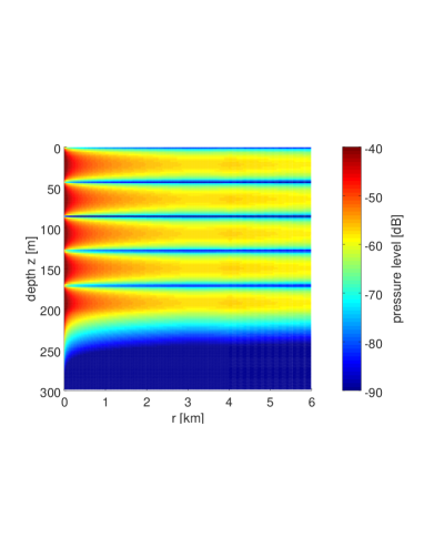
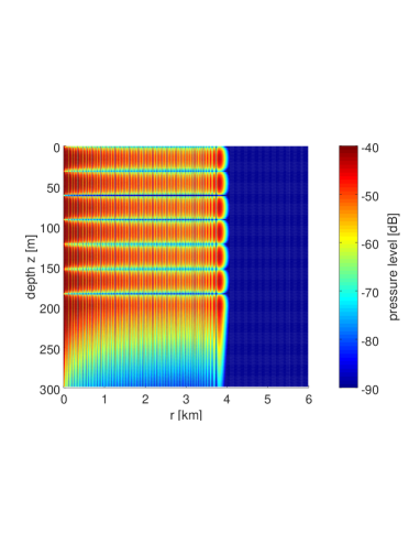
Figure 1: Pressure level, in dB re total spherical field at 1 m, of the field component given by mode 5 (left panel) and 7 (right panel), for the 2-D example, in the $rz$-plane. The symmetric source is at depth $z_{s}$ = 106 m and the frequency is 30 Hz.

Moreover, the mode 7 field exhibits a standing-wave interference pattern that is absent for mode 5. At cutoff, the modal energy turns back towards the source, with a focusing effect in this azimuthally symmetric environment. Hence, constructive as well as destructive interference arises between the out-going and in-coming field components. In the range-invariant $r<$ 3 km region, these field components are governed (with $m$=7) by the modal Hankel-function factors $H_{0}^{(1)}(k_{m}(r)r)$ and $H_{0}^{(2)}(k_{m}(r)r)$, respectively. Closer to $r$ = 4 km, where $k_{m}(r)$ is smaller, the period of the interference pattern is larger.

It is instructive to compare to the classical wedge examples by Jensen and Kuperman [9], with mode cutoff at upslope propagation in a homogeneous water column. Mode penetration into the bottom, rather than reflection back towards the source, showed up at cutoff in that study, which involved PE modeling and comparisons with tank experiments.

2.2 2-D PE approximation errors

For the cylindrically symmetric case, when the medium parameters do not depend on the polar $\theta$ coordinate, the 2-D Godin PE [10] for $\psi(r,z)=p(r,z)\,/\,H_{0}^{(1)}(k_{0}r)$, cf. [8, Eq. (3.130)], appears as

$$\frac{\partial\left(\rho^{-1/2}(I+X)^{1/4}\,\psi\right)}{\partial r}=ik_{0}\,\rho^{-1/2}\left((I+X)^{1/2}-I\right)(I+X)^{1/4}\,\psi\,.$$ (10)

It is valid outside the source at $r$ = 0 m. $I$ is the identity operator, $X=k_{0}^{-2}\,(\,\rho\,\partial(\rho^{-1}\partial/\partial z)/\partial z+(\omega^{2}/c^{2}-k_{0}^{2})\,)$, and $k_{0}$ is a reference wavenumber. With medium parameters according to Eqs. (4)- (5), and the local modes $Z_{m,0}(z)$ with modal wavenumbers $k_{m}(r)=(k_{m,0}^{2}+\omega^{2}S(r))^{1/2}$, $(I+X)(Z_{m,0})=(k_{m}/k_{0})^{2}\,Z_{m,0}$. Hence, it is natural to define the operators $(I+X)^{1/2}$ and $(I+X)^{1/4}$ by $(I+X)^{1/2}(Z_{m,0})=(k_{m}/k_{0})Z_{m,0}$ and $(I+X)^{1/4}(Z_{m,0})=(k_{m}/k_{0})^{1/2}\,Z_{m,0}$, respectively. With the mode expansion $\psi(r,z)=\sum_{m=1}^{\infty}\eta_{m}(r)\,Z_{m,0}(z)$, cf. Eq. (6), the PE (10) takes the form

$$\frac{d(R^{-1/2}(k_{m}/k_{0})^{1/2}\,\eta_{m})}{dr}=ik_{0}(k_{m}/k_{0}-1)R^{-1/2}(k_{m}/k_{0})^{1/2}\,\eta_{m}\ ,$$ (11)

where $m$ = 1,2,… Again, there is no mode coupling.

With accurate computation of the $\gamma_{m}(r)$ from Eq. (6), and their derivatives, it becomes possible to assess the errors of Eq. (11) and other PE approximations. Figure 2 shows the magnitude of the left-hand side of Eq. (11) for modes 5 and 7, for the 2-D example from Sec. 2.1. The relative errors of the right-hand side, compared to the left-hand side, are also included, as dashed curves. In each case, the reference wavenumber $k_{0}$ equals the pertinent modal wavenumber $k_{m,0}$, and $\gamma_{m}(r)/H_{0}^{(1)}(k_{0}r)$ replaces $\eta_{m}(r)$ at the evaluation of the two sides of Eq. (11).

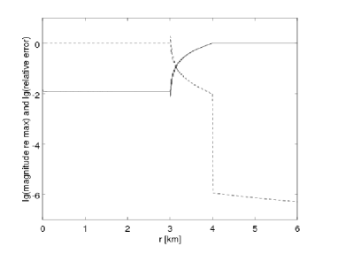
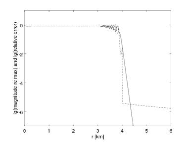
Figure 2: Solid curves: Magnitude of the left-hand side of Eq. (11), with $\gamma_{m}/H_{0}^{(1)}(k_{0}r)$ replacing $\eta_{m}$, for mode 5 (left panel) and 7 (right panel) in the 2-D example. The curve shows the logarithm of the magnitude divided by its maximum value. Dashed curves: Corresponding relative errors of the right-hand side of Eq. (11). The curve shows the logarithm of the relative error.

The significantly different characters of modes 5 and 7 are apparent also from Fig. 2. At $r<3$ km, where $k_{m}(r)$ is close to $k_{0}$, $d\left(\gamma_{m}(r)/H_{0}^{(1)}(k_{0}r)\right)/dr$ would be very small if there were no back-scattered or reflected field. At $r>4$ km, where there is no in-coming field, a large $d\left(\gamma_{m}(r)/H_{0}^{(1)}(k_{0}r)\right)/dr$ may arise from the mis-match between $k_{m}(r)$ and $k_{0}$. With weak back-scattering for mode 5, its $d\left(\gamma_{m}(r)/H_{0}^{(1)}(k_{0}r)\right)/dr$ is almost one hundred times stronger at $r>4$ km than at $r<3$ km. For mode 7, on the other hand, the strong back-scattering gives a large $d\left(\gamma_{m}(r)/H_{0}^{(1)}(k_{0}r)\right)/dr$ at $r<3$ km, and the cutoff at about $r$ = 4 km gives rise to an exponential decay beyond that range, also for $d\left(\gamma_{m}(r)/H_{0}^{(1)}(k_{0}r)\right)/dr$.

Turning to the relative PE approximation errors, they are of course very small in the out-going field regime beyond $r$ = 4 km, for both modes, and they decrease as the asymptotic approximation of the Hankel function improves with increasing range. At $r<$ 3 km, they are quite large, about 1 (100 %). This is not serious for mode 5 with its weak $d\left(\gamma_{m}(r)/H_{0}^{(1)}(k_{0}r)\right)/dr$ there, implying very small absolute errors. For mode 7 with its strong $d\left(\gamma_{m}(r)/H_{0}^{(1)}(k_{0}r)\right)/dr$ at $r<$ 3 km, however, this is clearly serious. A (one-way) PE model is not able to follow the standing-wave interference pattern for mode 7 in this case.

3 The 3-D case

From now on, consider particular media such that, cf. [6, Sec. 7.1.2],

$$\frac{1}{c^{2}(x,y,z)}=\frac{1}{c_{0}^{2}(z)}+S(x)\ ,$$ (12)

where (for convenience) $S(x_{s})=0$ s²/m². For simplicity, $\rho(x,y,z)=\rho_{0}(z)$ depends only on the depth $z$, and $S(x)$ is constant for large positive as well as large negative $x$. In particular, the medium parameters are independent of the $y$ coordinate.

As in Sec. 2, there is a free boundary at depth $z=0$ and a free or rigid boundary at depth $z_{h}$. The $Z_{m,0}(z)$, $m$ = 1,2,.., now form a complete set of orthogonal local modes at $x=x_{s}$ with corresponding modal wavenumbers $k_{m,0}$ and depth integrals $I_{m,0}$ by Eq. (8). The $Z_{m,0}(z)$ are local modes $Z_{m}(x,y,z)=Z_{m,0}(z)$ at other points $(x,y)$ in the horizontal plane too, with depth integrals $I_{m}(x,y)=I_{m,0}$ but with modal wavenumbers $k_{m}(x)=(k_{m,0}^{2}+\omega^{2}S(x))^{1/2}$. Expansion of the pressure $p$ in Eq. (2) in terms of the $Z_{m,0}$, i.e.,

$$p(x,y,z)=\sum_{m=1}^{\infty}\gamma_{m}(x,y)\,Z_{m,0}(z)\ ,$$ (13)

provides, after multiplication with $\rho_{0}^{-1}\,Z_{n,0}$ and integration over depth $z$, the 2-D horizontal refraction equations [8, Eq. (3.163)] (but with “$(x_{s})$” corrected to “$(\bm{x}_{s})$” in the right-hand side). The mode-separated Helmholtz-type horizontal refraction equations for the modal expansion coefficients $\gamma_{m}(x,y)$, $m$ = 1,2,.., are exact for the particular media under consideration.

Fourier transformation with respect to $y$ of the horizontal refraction equations yields

$$\gamma_{m}(x,y)=\int_{-\infty}^{\infty}\hat{\gamma}_{m}(x,\kappa)\exp(i\kappa y)\,d\kappa\ ,$$ (14)

where the functions $\hat{\gamma}_{m}(x,\kappa)$ fulfil ordinary differential equations. The ordinary differential equations for $\hat{\gamma}_{m}(x,\kappa)$ can be solved conveniently by 2$\times$2 propagator-matrix techniques as detailed in [8, Sec. 3.2.1.2], for example. Finally, adaptive integration with automatic error control [11] is convenient to compute the wavenumber integral in Eq. (14).

It is apparent how to use Eq. (14) for computation of field derivatives in connection with Eq. (13). Computation of energy flux requires first-order field derivatives. Specifically, the time-averaged energy-flux or intensity vector $\bm{\Phi}(\bm{x})$ is, by [12, Eqs. (1-11.11b)] and by [12, Eqs. (1-8.12)],

$$\bm{\Phi}(\bm{x})=\frac{1}{2\omega\rho(\bm{x})}\mathrm{Im}\left(p^{*}(\bm{x})\,\nabla p(\bm{x})\right)\ ,$$ (15)

where the asterisk denotes the complex conjugate.

3.1 Horizontal rays

Ray theory provides an approximate way to solve the 2-D horizontal refraction equations, that gives useful insight. The pertinent sound-speed profile in the horizontal $xy$-plane is, for mode $m$ and the angular frequency $\omega$, $c_{m}(x,\omega)$ as defined by

$$\frac{1}{c_{m}^{2}(x,\omega)}=\left(\frac{k_{m,0}(\omega)}{\omega}\right)^{2}+S(x)\ ,$$ (16)

emphasizing the frequency dependence in the notation. It is independent of $y$, and the ray tracing starts from $(x_{s},y_{s})$. Let $i(x)$ denote the angle between a ray at $x$, before it possibly turns, and the $x$ axis. With $\sigma$ as the Snell parameter of the ray, Snell’s law gives

$$\sin i(x)=\sigma\,c_{m}(x)=\frac{\sin i(x_{s})}{\left(1+(\frac{\omega}{k_{m,0}})^{2}\,S(x)\right)^{1/2}}\ ,$$ (17)

since $S(x_{s})=0$ s²/m². Hence, the ray turns when $S(x)=-(k_{m,0}/\omega)^{2}\,\cos i(x_{s})$. With the same ray directions $i(x_{s})$ at the source, a higher-order mode, with a smaller $k_{m,0}$, does not penetrate as deep into a high-velocity region as a lower-order mode does. When $S(x)$ is piece-wise linear, the rays are composed of parabolic segments and traveltimes along the rays can be computed analytically.

Consider horizontal rays of a certain type, concerning start direction towards increasing or decreasing $x$, number of turns etc., from $(x_{s},y_{s})$ to a fixed end point $(x_{e},y_{e})$ for mode $m$. The corresponding paths $\Gamma_{m}(\omega)$, Snell parameters $\sigma_{m}(\omega)$, and traveltimes $T_{m}(\omega)$ depend in general on the angular frequency $\omega$, since $k_{m,0}(\omega)/\omega$ does so. Apparently,

$$T_{m}(\omega)=\int_{\Gamma_{m}(\omega)}\frac{ds}{c_{m}(x,\omega)}$$ (18)

where $s$ is arc length. It follows from Fermat’s principle that

$$T_{m}(\omega+d\omega)=\int_{\Gamma_{m}(\omega)}\frac{ds}{c_{m}(x,\omega+d\omega)}+o(d\omega)\ .$$ (19)

Hence, by differentiation of Eq. (16) with respect to $\omega$,

$$\frac{dT_{m}(\omega)}{d\omega} = \int_{\Gamma_{m}(\omega)}\frac{dc_{m}^{-1}(x,\omega)}{d\omega}\,ds$$ (20)

$$= \frac{k_{m,0}(\omega)}{\omega^{2}}\left(\frac{dk_{m,0}(\omega)}{d\omega}-\frac{k_{m,0}(\omega)}{\omega}\right)\,\int_{\Gamma_{m}(\omega)}c_{m}(x,\omega)\,ds$$ (21)

$$= \frac{k_{m,0}(\omega)}{\omega^{2}}\left(\frac{dk_{m,0}(\omega)}{d\omega}-\frac{k_{m,0}(\omega)}{\omega}\right)\,\frac{|y_{e}-y_{s}|}{\sigma_{m}(\omega)}\ .$$ (22)

Propagator-matrix techniques [13], for example, can be used to compute the group slownesses $dk_{m,0}(\omega)/d\omega$.

According to the stationary-phase approximation, frequency components around $\omega$ interfere constructively at the group traveltime $t_{m}(\omega)$ defined by

$$t_{m}(\omega) = T_{m}(\omega)+\omega\,dT_{m}(\omega)/d\omega$$ (23)

$$= T_{m}(\omega)+\frac{k_{m,0}(\omega)}{\omega}\left(\frac{dk_{m,0}(\omega)}{d\omega}-\frac{k_{m,0}(\omega)}{\omega}\right)\frac{|y_{e}-y_{s}|}{\sigma_{m}(\omega)}\ .$$ (24)

The usual group-slowness result $t_{m}(\omega)=\left((x_{e}-x_{s})^{2}+(y_{e}-y_{s})^{2}\right)^{1/2}dk_{m,0}(\omega)/d\omega$ appears when $S(x)$ vanishes identically.

3.2 Example mimicking a 3-D wedge

An example mimicking a 3-D wedge appears by a modification of the example in Sec. 2.1. The same Pekeris wave-guide is present at the source position $(x_{s},y_{s})$ = (0,0) m, and the 30-Hz source is still at depth $z_{s}$ = 106 m.

Select a continuous $S(x)$, according to Eq. (12), such that the “water” sound speed increases to 1600 m/s at $x$ = 2.8 km and 1700 m/s at $x\geq$ 3.6 km. Furthermore, $S(x)$ is constant in $x\leq-3.6$ km, and it is linear in $-3.6$ km $<x<$ 2.8 km as well as in 2.8 km $<x<$ 3.6 km. It follows that the “water” and “sediment” sound speeds are 1395.3 and 2355.0 m/s, respectively, at $x\leq-3.6$ km, and that the “sediment” sound speed increases to 4177.9 m/s at $x$ = 2.8 km and 8876.9 m/s at $x\geq$ 3.6 km. Another choice of $S(x)$ could of course provide more realistic sound-speed values, but the present choice is preferable for the illustrations. Recall that the density $\rho(x,y,z)=\rho_{0}(z)$ is assumed to be independent of $x$ and $y$.

Figure 3 shows pressure levels, in dB re total spherical field at 1 m, at depth $z$ = 106 m in the horizontal $xy$-plane for the mode 3 and mode 7 field components. The high-velocity region for positive $x$ causes clear effects of horizontal refraction, particularly for the higher-order mode 7, cf. Eq. (17). Depth dependencies of the field, as shown in Fig. 4 for modes 3 and 7, are useful to verify the particular mode character. At $x$ = 0 m, the mode 3 and 7 contributions drop off significantly beyond about $y$ = 28 km and $y$ = 15 km, respectively. Indeed, Figs. 3 and 4 exhibit similar features as [4, Figs. 9-10] with 3-D PE solutions for a sloping-bottom wedge.

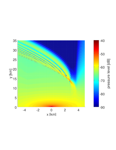
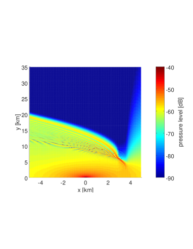
Figure 3: Pressure level, in dB re total spherical field at 1 m, of the field component given by mode 3 (left panel) and 7 (right panel), for the 3-D example, in the horizontal $xy$-plane at depth $z$ = 106 m. The symmetric source is at $(x_{s},y_{s},z_{s})$ = (0,0,106) m and the frequency is 30 Hz.

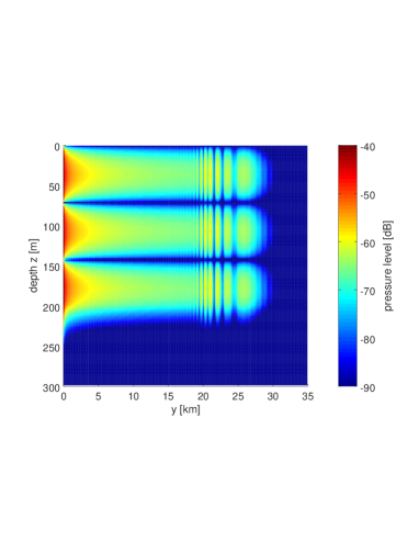
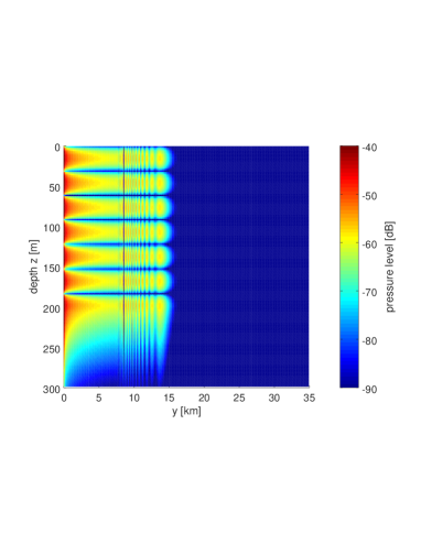
Figure 4: Pressure levels for modes 3 and 7 as in Fig. 3 but in the $yz$-plane at $x$ = 0 m.

The magnitudes of time-averaged energy flux for the mode 3 and mode 7 field components at depth 106 m, in dB re plane-wave pressure field of same strength as the total spherical field at 1 m, are rather similar to the pressure-level results in Fig. 3. Figure 5 shows the horizontal directions of the corresponding $\bm{\Phi}(\bm{x})$ vectors. (Their vertical components are negligible at the source depth.) As expected, the energy radiates more or less radially close to the source and at points $(x,y)$ with small $|y/x|$. The energy flux is in general directed to the left, towards decreasing $x$, in the shadow regions with weak fields, also in the right half-plane with $x>x_{s}$ = 0 m. In addition, there are beams with energy flux to the left starting at about $(x,y)$ = (3,13) km for the mode 3 field and at about $(x,y)$ = (3,6) km for the mode 7 field. At $x=-5$ km, these beams reach $y\approx$ 28 and 12 km, respectively.

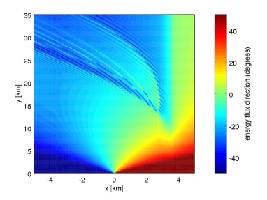
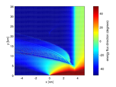
Figure 5: Horizontal direction of the time-averaged energy flux of the field component given by mode 3 (left panel) and 7 (right panel), for the 3-D example, in the horizontal $xy$-plane at depth $z$ = 106 m. Positive (negative) direction angles correspond to flux towards increasing (decreasing) $x$, and the angle 0^o indicates flux in the $y$-axis direction.

More ambitiously, it is possible to trace integral curves of a vector field given by $\bm{\Phi}(\bm{x})$ according to Eq. (15). Foreman [14] did this for some 2-D cases, introducing the term “exact rays” for the integral curves. In contrast to ordinary rays, such rays do not cross, since there is a unique direction at each point.

The mentioned beams with energy flux directed to the left are caused by horizontal refraction. Figure 6, with ordinary horizontal rays, provides further insight. The rays are traced for 30-Hz sound-speed profiles $c_{m}(x,\omega)$ with $m$ = 3 and 7, respectively, as defined by Eq. (16). In each case, there is a large-$y$ region with two ray arrivals to each point, separated from a shadow zone by a caustic ray envelope. At $x$ = 0 m, this region appears between about 20 and 28 km for mode 3, and between about 8 and 15 km for mode 7. The interference between the two arrivals gives rise to Lloyd-mirror type patterns [1] in Figs. 3 and 4. Moreover, the beams with energy flux directed to the left in Fig. 5 appear near the closest (smallest $y$) boundary of the corresponding interference region, and they are connected to ray turns at about $x$ = 3 km.

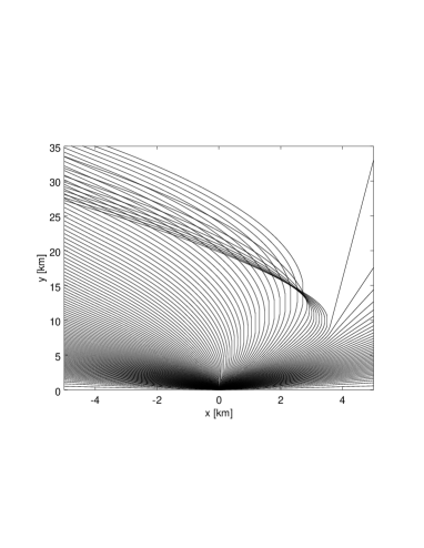
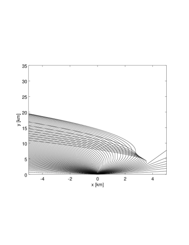
Figure 6: Ordinary horizontal rays for mode 3 (left panel) and 7 (right panel) at 30 Hz according to the corresponding sound-speed profile $c_{m}(x,\omega)$ as defined by Eq. (16).

It is also instructive to apply Fourier synthesis to produce the broad-band time traces in Fig. 7, for a short source pulse concentrated to the frequency band (3-dB limits) 28-40 Hz. (Because of the presence of lower frequency components, the truncation boundary at depth 1450 m is here lowered to 3450 m.) The additional solid (for 40 Hz) and dashed (for 28 Hz) curves show theoretical group traveltimes $t_{m}(\omega)$, computed by Eq. (24) for $m$ = 1, 3, 5. Modes 3 and 5 are apparently highly dispersive, and around $y$ = 22 km (selected for the right panel of Fig. 7), there are two arrivals for each of modes 1, 3, and 5. For modes 3 and 5, the dispersion causes a frequency beat pattern, since the instantaneous frequencies of the two arrivals may differ by a few Hz when they interfere. At some $y$ ranges, this gives the false impression that there are more than two arrivals for these modes.

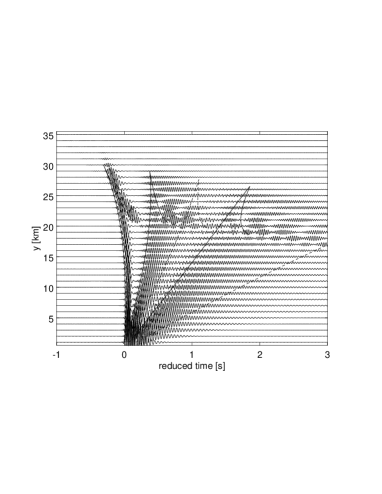
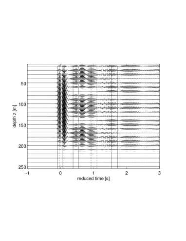
Figure 7: Time traces for the 3-D example with a short source pulse. The horizontal axis indicates reduced traveltime $t-y/c$, with $c$ = 1.5 km/s. The additional solid and dashed curves show theoretical group traveltimes at 40 and 28 Hz, respectively, for modes 1 (first), 3 (next), and 5 (last). Mode 7, which would arrive later, is not included. The time traces are at $(x,z)$ = (0,106) m for $y$ = 1,2,..,35 km in the left panel, and at $(x,y)$ = (0,22) km for $z$ = 10,20,..,250 m in the right panel. (At $(x,y)$ = (0,22) km, the theoretical reduced group traveltimes for mode 5 at 28 Hz are larger than 3 s.)

3.3 3-D PE approximation errors

Assuming $(x_{s},y_{s})$ = (0,0) m, return to the 2-D PE given by Eq. (10). In the 3-D context, it represents an N $\times$ 2-D PE approximation, ignoring horizontal refraction [1]. With laterally invariant density, sound-speed variation according to Eq. (12), local modes $Z_{m,0}(z)$ with modal wavenumbers $k_{m}(x)=(k_{m,0}^{2}+\omega^{2}S(x))^{1/2}$, and mode expansion according to $\psi(r,\theta,z)=\sum_{m=1}^{\infty}\eta_{m}(r,\theta)\,Z_{m,0}(z)$, cf. Eq. (13), the N $\times$ 2-D PE (10) takes the form

$$\frac{\partial((k_{m}/k_{0})^{1/2}\,\eta_{m})}{\partial r}=ik_{0}\,(k_{m}/k_{0}-1)(k_{m}/k_{0})^{1/2}\,\eta_{m}$$ (25)

for $m$ = 1,2,.., cf. Eq. (11). Using Fourier transformation according to Eq. (14) and wavenumber integration, it is now apparent how to evaluate the left- and right-hand sides of Eq. (25), and variants thereof, with $\gamma_{m}/H_{0}^{(1)}(k_{0}r)$ replacing $\eta_{m}$.

The left panel of Fig. 8 shows the relative errors of the right-hand side of Eq. (25) compared to the left-hand side, for the example from Sec. 3.2 and mode $m$ = 3. The reference wavenumber $k_{0}$ equals the corresponding modal wavenumber $k_{m,0}$.

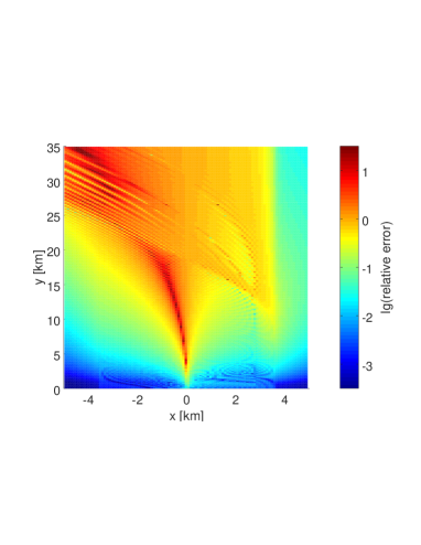
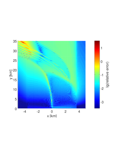
Figure 8: Left panel: Relative approximation errors of the N $\times$ 2-D PE (25) with $\gamma_{m}/H_{0}^{(1)}(k_{0}r)$ replacing $\eta_{m}$, for mode 3 in the 3-D example. The map shows the logarithm of the relative error. Right panel: Relative approximation errors of a certain 3-D PE.

Effects of horizontal refraction can be incorporated by amending the N $\times$ 2-D PE (10) with a term involving a Padé approximation of the operator $(I+Y)^{1/2}-I$, where $Y=(k_{0}r)^{-2}\,\partial^{2}/\partial\theta^{2}$ [4]. The two sides of the resulting 3-D PE may be multiplied by the involved Padé-approximation denominators. Significantly reduced relative errors appear in this way, as shown by the right panel of Fig. 8. For the part of the $xy$-plane that is shown, the area fraction where the relative PE approximation errors are greater than 0.1 decreases from 68 % for the left panel of Fig. 8 to 6 % for the right panel.

However, this 3-D PE is not always accurate enough and further improved 3-D PE approximations are of interest. The Chisholm rational approximant for two variables could be useful in this context [15].

4 Concluding remarks

The horizontal refraction equations for modal expansion coefficients are exact for the class of media with laterally invariant density and simple sound-speed variation according to Eq. (12), allowing separate (adiabatic) handling of the modes. The local modes do not vary among different horizontal positions, only the local modal wavenumbers do. After Fourier transformation with respect to one of the horizontal coordinates, wavenumber integration according to Eq. (14) provides accurate numerical solutions for each modal field and its spatial derivatives. With mild restrictions, there are explicit expressions for the integrand in terms of Airy and exponential functions. Computations of energy flux and horizontal rays help to understand the structure of the field, and the group traveltime result (24), for frequency-dependent ray paths, is thereby useful at broad-band applications.

For the azimuthally symmetric 2-D variant, with simple range dependence according to Eqs. (4) and (5), there are explicit expressions for the modal expansion coefficients in terms of Hankel and Airy functions, without any wavenumber integration. A restriction is that on each subinterval $(r_{1},r_{2})$, for a subinterval division of the range axis, the factor $R(r)$ is constant and the term $S(r)$ is either constant or of the form

$$S(r)=\frac{(r_{2}-r)S(r_{1})+(r-r_{1})S(r_{2})}{(r_{2}-r_{1})}+\frac{1}{4\omega^{2}}\left(\frac{1}{r_{1}}-\frac{1}{r}\right)\left(\frac{1}{r}-\frac{1}{r_{2}}\right)\left(1+\frac{r}{r_{1}}+\frac{r}{r_{2}}\right).$$ (26)

Thus, application of the explicit Airy-function expressions implies different $S(r)$ for different angular frequencies $\omega$. At broad-band computations, handled with Fourier synthesis, interpolation with short subintervals can mitigate the differences. With significant sound-speed increase with range, mode cutoff may appear (Sec. 2.1), much as at upslope propagation in a homogeneous water column. However, the corresponding modes are reflected back towards the source rather than lost by penetration into the bottom.

For the media according to Eqs. (4)- (5) or Eq. (12) with a laterally invariant density, the adiabatic-mode computation methods of Secs. 2 and 3 generate accurate reference solutions for PE-model verification. The important issue of mode coupling effects remains, however. Sections 2.2 and 3.3 include analysis examples for PE approximation errors. In this context, the errors concern the difference between the two sides of the PE (11) or (25) at insertion of Hankel-function scaled solutions of the Helmholtz-type equations (7) or the horizontal refraction equations, respectively. Significant improvements by full 3-D, rather than N $\times$ 2-D, computations show up in Sec. 3.3.

It is possible to solve the 2-D PE (11) as well as the N $\times$ 2-D PE (25) analytically. Considering the 2-D PE (11), for example, with a modal start solution at $r=r_{0}\geq 0$, where the medium is range-invariant in the interval $[0,r_{0}]$, its solution is

$$\eta_{m}(r)=\frac{R^{1/2}(r)}{R^{1/2}(r_{0})}\left(\frac{k_{m}(r_{0})}{k_{m}(r)}\right)^{1/2}\exp\left(i\int_{r_{0}}^{r}(k_{m}(u)-k_{0})\,du\right)\eta_{m}(r_{0})$$ (27)

for $m$ = 1,2,… Hence, it is easy to compare $\eta_{m}(r)$ and $\gamma_{m}(r)/H_{0}^{(1)}(k_{0}r)$ analytically, where $\gamma_{m}(r)$ solves Eq. (7). This is also true for variants of Eq. (11), with Padé approximations of the depth operators $(I+X)^{1/2}$ and $(I+X)^{1/4}$ in Eq. (10). A few examples appear in [8, Sec. 3.4.4].

References

- [1] F. B. Jensen, W. A. Kuperman, M. B. Porter, and H. Schmidt, Computational Ocean Acoustics. New York: Springer, 2nd ed., 2011.
- [2] R. B. Evans, “A coupled mode solution for acoustic propagation in a waveguide with stepwise depth variations of a penetrable bottom,” J. Acoust. Soc. Am., vol. 74, pp. 188–195, 1983.
- [3] J. A. Fawcett, “Modeling three-dimensional propagation in an oceanic wedge using parabolic equation methods,” J. Acoust. Soc. Am., vol. 93, pp. 2627–2632, 1993.
- [4] F. Sturm, “Numerical study of broadband sound pulse propagation in three-dimensional oceanic waveguides,” J. Acoust. Soc. Am., vol. 117, pp. 1058–1079, 2005.
- [5] J. A. Fawcett and T. W. Dawson, “Fourier synthesis of three-dimensional scattering in a two-dimensional oceanic waveguide using boundary integral integration methods,” J. Acoust. Soc. Am., vol. 88, pp. 1913–1920, 1990.
- [6] L. M. Brekhovskikh and O. A. Godin, Acoustics of Layered Media II. Berlin: Springer, 1992.
- [7] S. Ivansson, “Simple test cases with accurate numerical solutions for 3-D sound propagation modelling,” in Proceedings of the 4th Underwater Acoustics Conference and Exhibition, (Skiathos, Greece), pp. 609–616, September 3–8, 2017.
- [8] S. Ivansson, “Sound propagation modeling,” in Applied Underwater Acoustics (L. Bjørnø, T. Neighbors, and D. Bradley, eds.), ch. 3, pp. 185–272, Elsevier, 2017.
- [9] F. B. Jensen and W. A. Kuperman, “Sound propagation in a wedge-shaped ocean with a penetrable bottom,” J. Acoust. Soc. Am., vol. 67, pp. 1564–1566, 1980.
- [10] O. A. Godin, “Reciprocity and energy conservation within the parabolic approximation,” Wave Motion, vol. 29, pp. 175–194, 1999.
- [11] S. Ivansson and I. Karasalo, “A high-order adaptive integration method for wave propagation in range-independent fluid-solid media,” J. Acoust. Soc. Am., vol. 92, pp. 1569–1577, 1992.
- [12] A. D. Pierce, Acoustics. New York: Acoustical Society of America, 1991.
- [13] S. Ivansson, “The compound matrix method for multi-point boundary-value problems depending on a parameter,” Z. angew. Math. Mech., vol. 78, pp. 231–242, 1998.
- [14] T. L. Foreman, “An exact ray theoretical formulation of the Helmholtz equation,” J. Acoust. Soc. Am., vol. 86, pp. 234–246, 1989.
- [15] K. Lee and W. Seong, “Three dimensional acoustic parabolic equation based on Chisholm approximation with the splitting denominator,” J. Acoust. Soc. Am., vol. 141, p. 3589, 2017.