Egocentric Visitors Localization in Cultural Sites

Abstract.

We consider the problem of localizing visitors in a cultural site from egocentric (first person) images. Localization information can be useful both to assist the user during his visit (e.g., by suggesting where to go and what to see next) and to provide behavioral information to the manager of the cultural site (e.g., how much time has been spent by visitors at a given location? What has been liked most?). To tackle the problem, we collected a large dataset of egocentric videos using two cameras: a head-mounted HoloLens device and a chest-mounted GoPro. Each frame has been labeled according to the location of the visitor and to what he was looking at. The dataset is freely available in order to encourage research in this domain. The dataset is complemented with baseline experiments performed considering a state-of-the-art method for location-based temporal segmentation of egocentric videos. Experiments show that compelling results can be achieved to extract useful information for both the visitor and the site-manager.

1. Introduction

Cultural sites receive lots of visitors every day. To improve the fruition of cultural objects, a site manager should be able to assist the users during their visit by providing additional information and suggesting what to see next, as well as to gather information to understand the behavior of the visitors (e.g., what has been liked most) in order to improve the suggested visit paths or the placement of artworks. Traditional ways to achieve such goals include the employment of professional guides, the installation of informative panels, the distribution of printed material to the users (e.g., maps and descriptions) and the collection of visitors’ opinions through surveys. When the number of visitors grows large, the aforementioned traditional tools tend to become less effective, which motivates the employment of automated technologies. In order to assist visitors in a scalable and interactive way, site managers have employed technologies aimed at providing complementary information on the cultural objects on demand. An example of such technologies are audio guides, which allow to obtain spoken information about a point of interest by dialling the appropriate number on the device. Similarly, the use of tablets or smartphones allows to obtain audio-visual complementary information of an observed object of the cultural site by interacting with a touch interface (e.g., inserting the number of the cultural object of interest) or by taking a picture of a QR Code. Although effective in some cases, the aforementioned technologies are very limited by the following factors:

• they require the active intervention of the visitor, who needs to specify the correct number or to take a picture of the right QR Code;

• they require the site manager to install informative panels reporting the number or QR Code corresponding to a given cultural object (which is sometimes not possible due to the nature of the site).

Moreover, traditional systems are unable to acquire any information useful to understand the visitor’s habits or interests. To gather information about the visitors (i.e., what they see and where they are) in an automated way, past works have employed fixed cameras and classic “third person vision” algorithms to detect, track, count people and estimate their gaze (Bartoli et al., 2015). However, systems based on third person vision are capped by several limitations: 1) fixed cameras need to be installed in the cultural site and this is not always possible, 2) the fixed viewpoint of third person cameras makes it difficult to estimate what the visitors are looking at (e.g., ambiguity on estimation of what people see), 3) fixed cameras are easily affected by occlusion and people re-identification problems (e.g., difficulties to follow a person from a room to another), 3) the system has to work for several visitors at a time, making it difficult to profile them and to adapt its functioning to their specific needs (e.g., personal recommendation). Moreover, systems based on third person vision cannot easily communicate to the visitor in order to “augment his visit” providing information on the observed cultural object or by recommending what to see next.

Ideally, we would like to provide the user with an unobtrusive wearable device capable of addressing both tasks: augmenting the visit and inferring behavioral information about the visitors. We would like to note that wearable devices are particularly suited to solve this kind of tasks as they are naturally worn and carried by the visitor. Moreover, wearable systems do not require the explicit intervention of the visitor to deliver services such as localization, augmented reality and recommendation. The device should be aware of the current location of the visitor and capable to infer what he is looking at, and, ultimately, his behavior (e.g., what has already been seen? for how long?). Such a system would allow to provide automatic assistance to the visitor by showing him the current location, guiding him to a given area of the site, giving information about the currently observed cultural object, keeping track of what has been already seen and for how long, and suggesting what is yet to be seen by the visitor. Equipping multiple visitors with an egocentric vision device, it would be possible to track a profile of the different visitors in order to provide: 1) recommendations on what to see in the cultural site based on what has already been seen/liked (e.g, considering how much time has been spent at a given location or for how long the user has observed a cultural object), 2) statistics on the behaviors of the visitors within the site. Such statistics could be of great use by the site manager to improve the services offered by the cultural site and to facilitate the fruition of the cultural site.

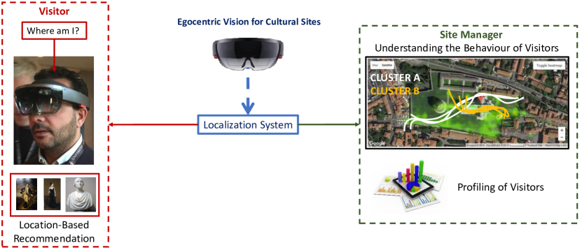
Figure 1. A diagram of a system which uses egocentric visitor localization to provide assistance to the user and augment his visit (left) and to provide useful information to the site manager (right).

As investigated by other authors (Cucchiara and Del Bimbo, 2014; Colace et al., 2014; Taverriti et al., 2016; Seidenari et al., 2017), wearable devices equipped with a camera such as smart glasses (e.g., Google Glass, Microsoft HoloLens and Magic Leap) offer interesting opportunities to develop the aforementioned technologies and services for visitors and site managers. Wearable glasses equipped with mixed reality visualization systems (i.e., capable of displaying virtual elements on images coming from the real world) such as Microsoft HoloLens and Magic Leap allow to provide information to the visitor in a natural way, for example by showing a 3D reconstruction of a cultural object or by showing virtual textual information next to a work of art. In particular, a wearable system should be able to carry out at least the following tasks: 1) localizing the visitor at any moment of the visit, 2) recognizing the cultural objects observed by the visitor, 3) estimating the visitor’s attention, 4) profiling the user, 5) recommending what to see next.

In this work, we address egocentric visitor localization, the first step towards the construction of a wearable system capable of assisting the visitor of a cultural site and collect information useful for the site management. In particular, we concentrate on the problem of room-based localization of visitors in cultural sites from egocentric visual data. As it is depicted in Figure 1, egocentric localization of visitors already enables different applications providing services to both the visitor and the site manager. In particular, localization allows to implement a “where am I” service, to provide the user which his own location in the cultural site and a location-based recommendation system. By collecting and managing localization information over time, the site manager will be able to profile visitors and understand their behavior. To study the problem we collected and labeled a large dataset of egocentric videos in the cultural site “Monastero dei Benedettini”, UNESCO World Heritage Site, which is located in Catania, Italy. The dataset has been acquired with two different devices and contains more than $4$ hours of video. Each frame has been labeled according to the location in which the user was located at the moment of data acquisition, as well as with the cultural object observed by the subject (if any). The dataset is publicly available for research purposes at http://iplab.dmi.unict.it/VEDI/.

We also report baseline results for the the problem of room-based localization on the proposed dataset. Experimental results point out that useful information such as the time spent in each location by visitors can be effectively obtained with egocentric systems.

The rest of the paper is organized as follows. In Section 2 we discuss the related work. The dataset proposed in this study is presented in Section 3. Section 4 revises the baseline approach for room-based localization of visitors in a cultural site. The experimental settings are reported in Section 5, while the results as well as a graphical interface to allow the analysis of the egocentric videos by the site manager are presented in Section 6. Section 7 concludes the paper.

2. Related Work

The use of Computer Vision to improve the fruition of cultural objects has been already investigated in past studies. Cucchiara and Del Bimbo discuss the use of computer vision and wearable devices for augmented cultural experiences in (Cucchiara and Del Bimbo, 2014). In (Colace et al., 2014) it is presented the design for a system to provide context aware applications and assist tourists. In (Taverriti et al., 2016) it is described a system to perform real-time object classification and artwork recognition on a wearable device. The system makes use of a Convolutional Neural Network (CNN) to perform object classification and artwork classification. In (Portaz et al., 2017a) is discussed an approach for egocentric image classification and object detection based on Fully Convolutional Networks (FCN). The system is adapted to mobile devices to implement an augmented audio-guide. In (Gallo et al., 2017), it is proposed a method to exploit georeferenced images publicly available on social media platforms to get insights on the behavior of tourists. In (Seidenari et al., 2017) is addressed the problem of creating a smart audio guide that adapts to the actions and interests of visitors. The system uses CNNs to perform object classification and localization and is deployed on a NVIDIA Jetson TK1. In  (Signorello et al., 2015) is investigated multimodal navigation of multimedia contents for the fruition of protected natural areas.

Visitors’ localization can be tackled outdoor using Global Positioning System (GPS) devices. These systems, however, are not suitable to localize the user in an indoor environment. Therefore, different Indoor Positioning Systems (IPS) have been proposed through the years (Curran et al., 2011). In order to retrieve accurate positions, these systems rely on devices such as active badges (Want and Hopper, 1992) and WiFi networks (Gu et al., 2009), which need to be placed in the environments and hence become part of the infrastructure. This operational way is not scalable since it requires the installation of specific devices, which is expensive and not always feasible, for instance, in the context of cultural heritage. Visual localization can be used to overcome many of the considered challenges. For instance, previous works addressed visual landmark recognition with smartphones (Amato et al., 2015; Weyand and Leibe, 2015; Li et al., 2017). In particular, the use of a wearable cameras allows to localize the user without relying on specific hardware installed in the cultural site. Visual localization can be performed at different levels, according to the required localization precision and to the amount of available training data. Three common levels of localization are scene recognition (Oliva and Torralba, 2001; Zhou et al., 2014), location recognition (Starner et al., 1998; Aoki et al., 1998; Torralba et al., 2003; Furnari et al., 2018) and 6-DOF camera pose estimation (Shotton et al., 2013; Kendall et al., 2015; Sattler et al., 2017). Some works also investigated the combination of classic localization based on non-visual sensors (such as bluetooth) with computer vision (Ishihara et al., 2017a, b).

In this work, we concentrate on location recognition, since we want to be able to recognize the environment (e.g., room) in which the visitor is located. Location recognition is the ability to recognize when the user is moving in a specific space at the instance level. In this case the egocentric (first person) vision system should be able to understand if the user is in a given location. Such location can either be a room (e.g., office 368 or exhibition room 3) or a personal space (e.g., office desk). In order to setup a location recognition system, it is usually necessary to acquire a moderate amount of visual data covering all the locations visited by the user. Visual location awareness has been investigated by different authors over the years. In (Starner et al., 1998) has been addressed the recognition of basic tasks and locations related to the Patrol game from egocentric videos in order to assist the user during the game. The system was able to recognize the room in which the user was operating using simple RGB color features. An Hidden Markov Model (HMM) was employed to enforce the temporal smoothness of location predictions over time. In  (Aoki et al., 1998), it is proposed a system to recognize personal locations from egocentric video using the approaching trajectories observed by the wearable camera. At training time the system built a dictionary of visual trajectories (i.e., collections of images) captured when approaching each specific location. At test time, the observed trajectory was matched to the dictionary in order to detect the current location. In  (Torralba et al., 2003), it has been designed a context-based vision system for place and scene recognition. The system used an holistic visual representation similar to GIST to detect the current location at the instance level and recognize the scene category of previously unseen environment. Other authors (Xu et al., 2014) proposed a way to provide context-aware assistance for indoor navigation using a wearable system. When it is not possible to acquire data for all the locations which might be visited by the user, it is generally necessary to explicitly consider a rejection option, as proposed in (Furnari et al., 2018).

Some authors proposed datasets to investigate different problems related to cultural sites. For instance, In  (Portaz et al., 2017a, b), it is proposed a dataset of images acquired by using classic or head-mounted cameras. The dataset contains a small number of images and is intended to address the problem of image search (e.g., recognizing a painting). In (Bartoli et al., 2015), is presented a dataset acquired inside the National Museum of Bargello in Florence. The dataset (acquired by 3 fixed IPcameras) is intended for pedestrian and group detection, gaze estimation and behavior understanding.

To the best of our knowledge, this paper introduces the first large scale public dataset acquired in a cultural site using wearable cameras which is intended for egocentric visitor localization research purposes.

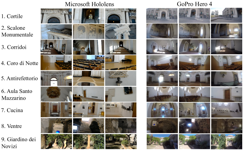
Figure 2. The figure shows some frames for each considered environment, acquired with Microsoft Hololens (left column) and GoPro Hero4 (right column) wearable devices.

3. Dataset

We collected a large dataset of videos acquired in the Monastero dei Benedettini, located in Catania, Italy. The dataset has been acquired using two wearable devices: a head-mounted Microsoft HoloLens and a chest-mounted GoPro Hero4. The considered devices represent two popular choices for the placement of wearable cameras. Indeed, chest-mounted devices generally allow to produce better quality images due to the reduced egocentric motion with respect to head-mounted devices. On the other side, head-mounted cameras allow to capture what the user is looking at and hence they are better suited to model the attention of the user. Moreover, head-mounted devices such as HoloLens allow for the use of augmented reality, which can be useful to assist the visitor of a cultural site. The two devices are also characterized by two different Field Of View (FOV). In particular, the FOV of the HoloLens device is narrow-angle, while the FOV of the GoPro device is wide-angle. This is shown in Figure 2, which reports some frames acquired with HoloLens along with the corresponding images acquired with GoPro. Since we would like to assess which device is better suited to address the localization problem, we use the two devices simultaneously during the data acquisition procedure in order to collect two separate and compliant datasets: one containing only data acquired with HoloLens device and the other one containing only data acquired using the GoPro device. The videos captured by HoloLens device have a resolution equal to $1216\times 684$ pixels and a frame rate of $24$ fps, whereas the videos recorded with GoPro Hero 4 have a resolution of $1280\times 720$ pixels and a frame rate of $25$ fps.

Each video frame has been labeled according to: 1) the location of the visitor and 2) the “point of interest” (i.e. the cultural object) observed by the visitor, if any. In both cases, a frame can be labeled as belonging to a “negative” class, which denotes all visual information which is not of interest. For example, a frame is labeled as negative when the visitor is transiting through a corridor which has not been included in the training set because is not a room (context) of interest for the visitors or when he is not looking at any of the considered points of interest. We considered a total of $9$ environments and $57$ points of interests. Each environment is identified by a number from $1$ to $9$, while points of interest (i.e., cultural objects) are denoted by a code in the form $X.Y$ (e.g., $2.3$), where $X$ denotes the environment in which the points of interest are located and $Y$ identify the point of interest. Figure 2 shows some representative samples for each of the $9$ considered environments. Table 1 shows the list of the considered environments (left column) and the related points of interest (right column). In the case of class Cortile, the same video is used to represent both the environment (1) and the related point of interest (Ingresso - 1.1). Figure 3 shows some representative samples of the $57$ points of interest acquired with HoloLens and GoPro Hero 4, whereas Figure 4 reports some sample frames belonging to negative locations and points of interest. As can be noted from the reported samples, the GoPro device allow to acquire a larger amount of visual information, due to its wide-angle field of view. On the contrary, data acquired using the HoloLens device tends to exhibit more visual variability, due to the head-mounted point of view, which suggests its better suitability for the recognition of objects of interest and behavioral understanding.

Environments	Points of Interest		Environments	Points of Interest
Cortile (1)	Ingresso (1.1)			PavimentoOriginale (6.3)
Scal. Monumentale (2)	RampaS.Nicola (2.1)			PavimentoRestaurato (6.4)
	RampaS.Benedetto (2.2)			BassorilieviMancanti (6.5)
	SimboloTreBiglie (3.1)		Aula S.Mazzarino (6)	LavamaniSx (6.6)
	ChiostroLevante (3.2)			LavamaniDx (6.7)
	Plastico (3.3)			TavoloRelatori (6.8)
	Affresco (3.4)			Poltrone (6.9)
	Finestra_ChiostroLev. (3.5)			Edicola (7.1)
Corridoi (3)	PortaCorodiNotte (3.6)			PavimentoA (7.2)
	TracciaPortone (3.7)			PavimentoB (7.3)
	StanzaAbate (3.8)		Cucina (7)	PassavivandePav.Orig. (7.4)
	CorridoioDiLevante (3.9)			AperturaPavimento (7.5)
	CorridoioCorodiNotte (3.10)			Scala (7.6)
	CorridoioOrologio (3.11)			SalaMetereologica (7.7)
	Quadro (4.1)			Doccione (8.1)
Coro di Notte (4)	PavimentoOrig.Altare (4.2)			VanoRaccoltaCenere (8.2)
	BalconeChiesa (4.3)			SalaRossa (8.3)
	PortaAulaS.Mazzarino (5.1)			ScalaCucina (8.4)
	PortaIng.MuseoFabb. (5.2)			CucinaProvv. (8.5)
	PortaAntirefettorio (5.3)		Ventre (8)	Ghiacciaia (8.6)
	PortaIngressoRef.Piccolo (5.4)			Latrina (8.7)
Antirefettorio (5)	Cupola (5.5)			OssaeScarti (8.8)
	AperturaPavimento (5.6)			Pozzo (8.9)
	S.Agata (5.7)			Cisterna (8.10)
	S.Scolastica (5.8)			BustoPietroTacchini (8.11)
	ArcoconFirma (5.9)			NicchiaePavimento (9.1)
	BustoVaccarini (5.10)		Giardino Novizi (9)	TraccePalestra (9.2)
Aula S.Mazzarino (6)	Quadro S.Mazzarino (6.1)			PergolatoNovizi (9.3)
	Affresco (6.2)

Table 1. The table reports the list of all environments and the related points of interest contained. In parenthesis, we report the unique numerical code of the environment/point of interest.

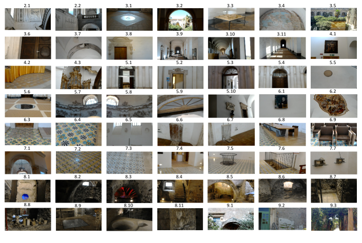
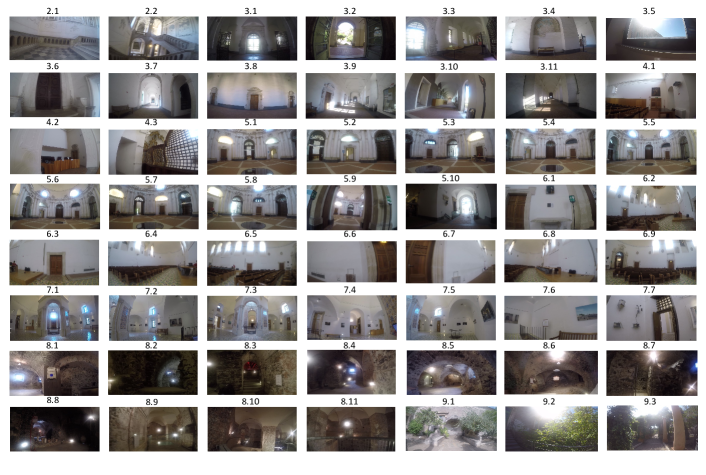
Figure 3. The figure shows a sample frame for each of the $57$ points of interest acquired with both Microsoft Hololens (top) and GoPro (bottom).

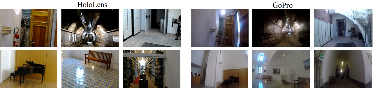
Figure 4. Example of frames belonging to the negative class, acquired with Microsoft Hololens (left) and GoPro (right).

The dataset is composed of separate training and test videos, which have been collected following two different modalities. To collect the training set, we acquired a set of videos (at least one) for each of the considered environments and a set of videos for each of the considered points of interest. Environment-related training videos have been acquired by an operator who had been instructed to walk into the environment and look around to capture images from different points of view. A similar procedure is employed to acquire training videos for the different points of interest. In this case, the operator has been instructed to walk around the object and look at it from different points of view. For each camera, we collected a total of $12$ training videos for the $9$ environments and $68$ videos for the $57$ points of interest. This accounts to a total of $80$ training videos for each camera. Table 2 summarizes the number of training videos acquired for each environment.

Environment	#Videos	#Frames
1 Cortile	1	1171
2 Scalone Monumentale	6	13464
3 Corridoi	14	31037
4 Coro di Notte	7	12687
5 Antirefettorio	14	29918
6 Aula Santo Mazzarino	10	31635
7 Cucina	10	31112
8 Ventre	14	68198
9 Giardino dei Novizi	4	10852
Total	80	230074

Table 2. Training videos and total number of frames for each environment.

The test videos have been acquired by operators who have been asked to simulate a visit to the cultural site. No specific information on where to move, what to look, and for how long have been given to the operators. Test videos have been acquired by three different subjects. Specifically, we acquired $7$ test video per wearable camera, totaling $14$ test videos. Each HoloLens video is composed by one or more video fragments due to the limit of recording time imposed by the default Hololens video capture application. Table 3 reports the list of test videos acquired using HoloLens and GoPro devices. For each test video, we report the number of frames and the list of environments the user visits during the acquisition of the video.

HoloLens				GoPro
Name	#Frames	Environments		Name	#Frames	Environments
Test1.0	7202	1 - 2 - 3 - 4 - 5 - 6		Test1	14788	1 - 2 - 3 - 4
Test1.1	7202			Test2	10503	1 - 2 - 3 - 5
Test2.0	7203	1 - 2 - 3 - 4		Test3	14491	1 - 2 - 3 - 5 - 9
Test3.0	7202			Test4	36808	1 - 2 - 3 - 4 - 5 - 6 - 7 - 8 - 9
Test3.1	7203			Test5	18788	1 - 2 - 3 - 5 - 7 - 8
Test3.2	7201	1 - 2 - 3 - 4 - 5 - 6 - 7 - 8 - 9		Test6	12661	2 - 3 - 4 - 8 - 9
Test3.3	7202			Test7	38725	1 - 2 - 3 - 4 - 5 - 6 - 7 - 8 - 9
Test3.4	5694			Total	146764
Test4.0	7204
Test4.1	7202
Test4.2	3281	1 - 2 - 3 - 4 - 5 - 7 - 8 - 9
Test4.3	7202
Test4.4	4845
Test5.0	6590	1 - 2 - 3 - 4 - 5 - 6 - 7 - 8 - 9
Test5.1	7202
Test5.2	7202
Test5.3	7201
Test6.0	7202	1 - 2 - 3
Test7.0	7202	1 - 2 - 3 - 5
Test7.1	2721
Total	131163

Table 3. The list of test videos acquired using HoloLens (left) and GoPro (right). For each video, we report the number of frames and the list of environments visited by the user during the acquisition. The last rows report the total number of frames.

The dataset, which we call UNICT-VEDI, is publicly available at our website: http://iplab.dmi.unict.it/VEDI/. The reader is referred to the supplementary material at the same page for more details about the dataset.

4. Egocentric Localization in a Cultural Site

We perform experiments and report baseline results related to the task of localizing visitors from egocentric videos. To address the localization task, we consider the approach proposed in  (Furnari et al., 2018). This method is particularly suited for the considered task since it can be trained with a small number of samples and includes a rejection option to determine when the visitor is not located in any of the environments considered at training time (i.e., when a frame belongs to the negative class). Moreover, as detailed in (Furnari et al., 2018), the method achieves state of the art results on the task of location-based temporal video segmentation, outperforming classic methods based on SVMs and local feature matching. At test time, the algorithm segments an egocentric video into temporal segments each associated to either one of the “positive” classes or, alternatively, the “negative” class. The approach is reviewed in the following section. The reader is referred to (Furnari et al., 2018) for more details.

4.1. Method Review

At training time, we define a set of $M$ “positive” classes, for which we provide labeled training samples. In our case, this corresponds to the set of training videos acquired for each of the considered environments. At test time, an input egocentric video $\mathcal{V}=\{F_{1},\ldots,F_{N}\}$ composed by $N$ frames $F_{i}$ is analyzed. Each frame of the video is assumed to belong to either one of the considered $M$ positive classes or none of them. In the latter case, the frame belongs to the “negative class”. Since, negative training samples are not assumed at training time, the algorithm has to detect which frames do not belong to any of the positive classes and reject them. The goal of the system is to divide the video into temporal segment, i.e., to produce a set of $P$ video segments $\mathcal{S}=\{s_{i}\}_{1\leq i\leq P}$, each associated with a class (i.e., the room-level location). In particular, each segment is defined as $s_{i}=\{s_{i}^{s},s_{i}^{e},s_{i}^{c}\}$, where $s_{i}^{s}$ represents the staring frame of the segment, $s_{i}^{e}$ represents the ending frame of the segments and $s_{i}^{c}\in\{0,\ldots,M\}$ represents the class of the segment ($s_{i}^{c}=0$ is the “negative class”, while $s_{i}^{c}=1,\ldots,M$ represent the “positive” classes).

The temporal segmentation of the input video is achieved in three steps: discrimination, negative rejection and sequential modeling. Figure 5 shows a diagram of the considered method, including typical color-coded representations of the intermediate and final segmentation output.

In the discrimination step, each frame of the video $F_{i}$ is assigned the most probable class $y^{*}_{i}$ among the considered $M$ positive classes. In order to perform such assignment, a multi-class classifier trained only on the positive samples is employed to estimate the posterior probability distribution:

(1) $$P(y_{i}|F_{i},y_{i}\neq 0)$$

where $y_{i}\neq 0$ indicates that the negative class is excluded from the posterior probability. The most probable class $y^{*}_{i}$ is hence assigned using the Maximum A Posteriori (MAP) criterion: $y^{*}_{i}=\arg\max_{y_{i}}P(y_{i}|I_{F},y_{i}\neq 0)$. Please note that, at this stage, the negative class is not considered. The discrimination step allows to obtain a noisy assignment of labels to the frames of the input video, as it is depicted in Figure 5.

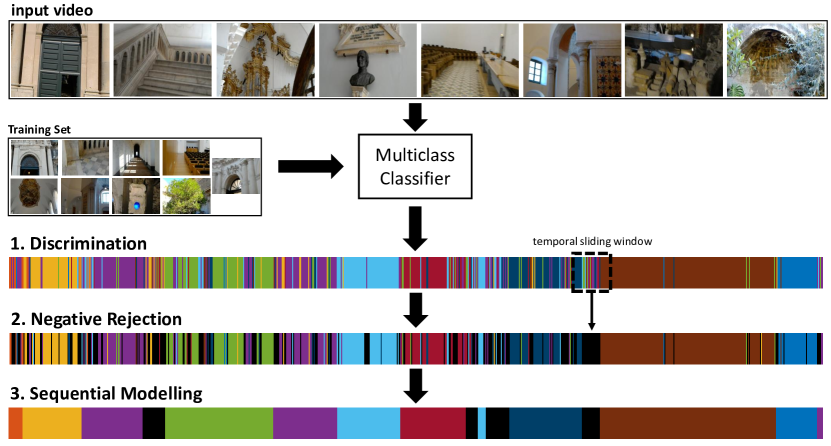
Figure 5. Diagram of the considered room-based localization method consisting in three steps: 1) Discrimination, 2) Negative Rejection, 3) Sequential Modeling.

The negative rejection step aims at identifying regions of the video in which frames are likely to belong to the negative class. Since in an egocentric video locations are deemed to change smoothly, regions containing negative frames are likely to be characterized by noisy class assignments. This is expected since the multi-class classifier used in the discrimination step had no knowledge of the negative class. Moreover, consecutive frames of an egocentric video are likely to contain uncorrelated visual content, due to fast head movements, which would lead the multi-class classifier to pick a different class for each negative frame. To leverage this consideration, the negative rejection step quantifies the probability of each frame to belong to the negative class by estimating the variation ratio (a measure of entropy) of the nominal distribution of the assigned labels in a neighborhood of size $K$ centered at the frame to be classified. Let $\mathcal{Y}_{i}^{K}=\{y_{i-\lfloor\frac{K}{2}\rfloor},\ldots,y_{i+\lfloor\frac{K}{2}\rfloor}\}$ be the set of positive labels assigned to the frames comprised in a neighborhood of size $K$ centered at frame $F_{i}$. The rejection probability for the frame $F_{i}$ is computed as the variation ratio of the sample $\mathcal{Y}_{i}^{K}$:

(2) $$P(y_{i}=0|F_{i})=1-\frac{\sum_{k=i-\lfloor\frac{K}{2}\rfloor}^{i+\lfloor\frac{K}{2}\rfloor}{[y_{k}=mode(\mathcal{Y}_{i}^{K})]}}{K}$$

where $[\cdot]$ is the Iverson bracket, $y_{k}\in\mathcal{Y}_{i}^{K}$ and $mode(\mathcal{Y}_{i}^{K})$ is the most frequent label of $\mathcal{Y}_{i}^{K}$. Since $y_{i}=0$ and $y_{i}\neq 0$ are disjoint events, the posterior probability defined in Equation (1) can be easily merged to the probability defined in Equation (2) to estimate the posterior probability $P(y_{i}|F_{i})$. Note that this is a posterior probability over the $M$ positive classes, plus the negative one. The MAP criterion can be used to assign each frame $F_{i}$ the most probable class $y_{i}$ using the posterior probability $P(y_{i}|F_{i})$ (see  Figure 5). Please note that, in this case, the assigned labels include the negative class.

The label assignment obtained in the negative rejection step is still a noisy one (see Figure 5). The sequential modeling step smooths the segmentation result enforcing temporal coherence among neighboring predictions. This is done employing a Hidden Markov Model (HMM) (Bishop, 2006) with $M+1$ states ($M$ “positive” classes plus the “negative” one). The HMM models the conditional probability of the labels $\mathcal{L}=\{y_{1},\ldots,y_{N}\}$ given the video $\mathcal{V}$:

(3) $$P(\mathcal{L}|\mathcal{V})\propto\prod_{i=2}^{N}P(y_{i}|y_{i-1})\prod_{i=1}^{N}P(y_{i}|F_{i})$$

where $P(y_{i}|I_{i})$ models the emission probability (i.e., the probability of being in state $y_{i}$ given the frame $F_{i}$). The state transition probabilities $P(y_{i}|y_{i-1})$ are modeled defining an “almost identity matrix” which encourages the model to rarely allow for state changes:

(4) $$P(y_{i}|y_{i-1})=\begin{cases}\varepsilon,&\mbox{if }y_{i}\neq y_{i-1}\\ 1-M\varepsilon,&\mbox{otherwise}\end{cases}$$

The definition above depends on a parameter $\varepsilon$ which controls the amount of smoothing in the predictions. The optimal set of labels $\mathcal{L}$ according to the defined HMM can be obtained using the Viterbi algorithm (see Figure 5 - 3. Sequential Modeling). The segmentation $\mathcal{S}$ is finally obtained by considering the connected components of the optimal set of labels $\mathcal{L}$.

5. Experimental Settings

In this section, we discuss the experimental settings used for the experiments. To assess the potential of the two considered devices, we perform experiments separately on data acquired using HoloLens and GoPro by training and testing two separate models.

To setup the method reviewed in Section 4, it is necessary to train a multi-class classifier to discriminate between the $M$ positive classes (i.e., environments). We implement this component fine-tuning a VGG19 Convolutional Neural Network (CNN) pre-trained on the ImageNet dataset (Simonyan and Zisserman, 2014) to discriminate between the $9$ considered classes (Cortile, Scalone Monumentale, Corridoi, Coro di Notte, Antirefettorio, Aula Santo Mazzarino, Cucina, Ventre e Giardino dei Novizi). To compose our training set, we first considered all image frames belonging to the training videos collected for each environment (Figure 2). We augment the frames of each of the considered environments including also frames from the training videos collected for the points of interest contained in the environment. We finally select exactly $10000$ frames for each class, except for the “Cortile” (1) class which contained only $1171$ frames (in this case all frames have been considered). As previously discussed, the same video is used for both the environment “Cortile” (1) and point of interest Ingresso (1.1). Therefore, it was not possible to gather more frames from videos related to the points of interest. To validate the performances of the classifier, we randomly select $30\%$ of the training samples to obtain a validation set. Please note that the CNN classifier is trained solely on positive data and no negatives are employed at this stage. To select the optimal values for the parameters $K$ (neighborhood size for negative rejection) and $\varepsilon$ (HMM smoothing parameter), we carry out a grid search on one of the test videos, which is used as “validation video”. Specifically, we consider $K\in\{50,100,300\}$ and $\varepsilon\in[10^{-300},10^{-2}]$ for the grid search. We select “Test 3” as a validation video for the algorithms trained on data acquired with HoloLens and “Test 4” for the experiments related to data acquired using the GoPro camera. These two videos are selected since they contain all the classes and, overall, similar content (see Table 3). Moreover, the two videos have been acquired simultaneously by the same operator to provide similar material for validation. The grid search led to the selection of the following parameter values: $K=50;\varepsilon=10^{-152}$ in the case of the experiments performed on HoloLens data and $K=300;\varepsilon=10^{-171}$ for the experiments performed on the GoPro data. We used the Caffe framework (Jia et al., 2014) to train the CNN models. All the data, code and trained models useful to replicate the work are publicly available for download at our web page http://iplab.dmi.unict.it/VEDI/.

All experiments have been evaluated according to two complementary measures: $FF_{1}$ and $ASF_{1}$ (Furnari et al., 2018). The $FF_{1}$ is a frame-based measure obtained computing the frame-wise $F_{1}$ score for each class. This measure essentially assesses how many frames have been correctly classified without taking into account the temporal structure of the prediction. A high $FF_{1}$ score indicates that the method is able to estimate the number of frames belonging to a given class in a video. This is useful to assess, for instance, how much times has been spent at a given location, regardless the temporal structure. To assess how well the algorithm can split the input videos into coherent segments, we also use the $ASF_{1}$ score, which measures how accurate the output segmentation is with respect to ground truth. $FF_{1}$ and $ASF_{1}$ scores are computed per class. We also report overall $mFF_{1}$ and $mASF_{1}$ scores obtained by averaging class-related scores. The reader is referred to (Furnari et al., 2018) for details on the implementation of such scores. An implementation of these measures is available at the following link: http://iplab.dmi.unict.it/PersonalLocationSegmentation/.

Class Test1 Test2 Test4 Test5 Test6 Test7 AVG 1 Cortile 0.94 0.00 0.93 0.00 0.95 0.77 0.59 2 Scalone Monumentale 0.99 0.98 0.99 0.95 0.98 0.85 0.96 3 Corridoi 0.93 0.93 0.95 0.85 0.99 0.85 0.92 4 Coro Di Notte 0.94 0.94 0.89 0.87 / / 0.91 5 Antirefettorio 0.94 / 0.96 0.94 / 0.94 0.95 6 Aula Santo Mazzarino 0.99 / / 0.98 / / 0.99 7 Cucina / / 0.65 0.75 / / 0.70 8 Ventre / / 0.92 0.99 / / 0.96 9 Giardino dei Novizi / / 0.95 0.71 / / 0.83 Negatives 0.56 0.50 0.26 0.37 / / 0.42 $mFF_{1}$ 0.90 0.67 0.83 0.74 0.97 0.85 0.82

Table 4. Frame-based $FF_{1}$ scores of the considered method on data acquired using the HoloLens device. The “/” sign indicates that no samples from that class were present in the test video.

Class Test1 Test2 Test4 Test5 Test6 Test7 AVG 1 Cortile 0.89 0.00 0.86 0.00 0.90 0.62 0.48 2 Scalone Monumentale 0.97 0.95 0.97 0.86 0.97 0.74 0.90 3 Corridoi 0.85 0.87 0.84 0.69 0.99 0.58 0.79 4 Coro Di Notte 0.81 0.90 0.78 0.31 / / 0.66 5 Antirefettorio 0.88 / 0.93 0.66 / 0.90 0.83 6 Aula Santo Mazzarino 0.99 / / 0.96 / / 0.96 7 Cucina / / 0.48 0.57 / / 0.53 8 Ventre / / 0.85 0.99 / / 0.92 9 Giardino dei Novizi / / 0.90 0.66 / / 0.78 Negatives 0.50 0.39 0.12 0.3 / / 0.27 $mASF_{1}$ 0.84 0.62 0.71 0.60 0.95 0.71 0.71

Table 5. Segment-based $ASF_{1}$ scores of the considered method on data acquired using the HoloLens device. The “/” sign indicates that no samples from that class were present in the test video.

6. Results

Table 4 and Table 5 report the $mFF_{1}$ and $mASF_{1}$ scores obtained using data acquired using the HoloLens device. Please note that all algorithms have been trained using only training data acquired with the HoloLens device (no GoPro data has been used). “Test 3” is excluded from the table since it has been used for validation. The tables report the $FF_{1}$ and $ASF_{1}$ scores for each class and each test video, average per-class $FF_{1}$ and $ASF_{1}$ scores across videos, overall $mFF_{1}$ and $mASF_{1}$ scores for each test video and the average $mFF_{1}$ and $mASF_{1}$ scores which summarize the performances over the whole test set. As can be noted from both tables, some environments such as “Cortile”, “Cucina” and “Giardino dei Novizi” are harder to recognize than others. This is due to the greater variability characterizing such environments. In particular, “Cortile” and “Giardino dei Novizi” are outdoor environments, while all the others are indoor environments. It should be noted that, as discussed before, the two considered measures ($mFF_{1}$ and $mASF_{1}$) capture different abilities of the algorithm. For instance, some environments (e.g., “Corridoi” and “Coro di Notte”) report high $mFF_{1}$, and lower $mASF_{1}$. This indicates that the method is able to quantify the overall amount of time spent at the considered location, but temporal structure of the segments is not correctly retrieved. The average $mASF_{1}$ of $0.71$ and $mFF_{1}$ of $0.83$ obtained over the whole test set indicate that the proposed approach can be already useful to provide localization information to the visitor or for later analysis, e.g., to estimate how much time has been spent by a visitor at a given location, how many times a given environment has been visited, or what are the paths preferred by visitors.

Figure 6 reports the confusion matrix of the system on the HoloLens test set. The confusion matrix does not include frames from the “Test 3” video, which has been used for validation. The matrix confirms how some distinctive environments are well recognized, while others are more challenging. The matrix also suggests that most of the error is due to the challenging rejection of negative samples. Other minor source of errors are the “Giardino dei Novizi - Corridoi”, “Cortile - Scalone Monumentale” and “Coro di Notte - Corridoi” class pairs. We note that the considered pairs are neighboring locations, which suggests that the error is due to small inaccuracies in the temporal segmentation.

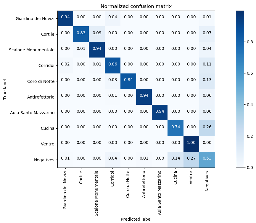
Figure 6. Confusion matrix of the considered method trained and tested on the HoloLens data.

We also report experiments performed on the GoPro data. To compare the effects of using different acquisition devices and wearing modalities, we replicate the same pipeline used for the experiments reported in the previous section. Hence, we trained and tested the same algorithms on data acquired using the GoPro device.

Table 6 and Table 7 report the $mFF_{1}$ and $mASF_{1}$ scores for the test videos acquired using the GoPro device. Results related to the “Test 4” validation video are excluded from the tables. The method allows to obtain overall similar performances for the different devices (an average $mFF_{1}$ score of $0.81$ in the case of GoPro, vs $0.82$ in the case of HoloLens and an average $mASF_{1}$ score of $0.71$ vs $0.71$). However, $mFF1$ performances on the single test videos are distributed differently (e.g., “Test 1” has a $mFF_{1}$ score of $0.90$ in the case of HoloLens data and a $mFF_{1}$ score of $0.67$ in the case of GoPro data).

Class Test1 Test2 Test3 Test5 Test6 Test7 AVG 1 Cortile 0.00 0.97 0.95 0.92 / 0.00 0.57 2 Scalone Monumentale 0.92 0.92 0.99 0.99 0.96 0.90 0.95 3 Corridoi 0.90 0.97 0.99 0.99 0.97 0.98 0.97 4 Coro Di Notte 0.89 / / / 0.98 0.88 0.92 5 Antirefettorio / 0.99 0.98 0.96 / 0.87 0.95 6 Aula Santo Mazzarino / / / / / 0.90 0.90 7 Cucina / / / 0.89 / 0.83 0.86 8 Ventre / / / 0.99 0.67 0.97 0.88 9 Giardino dei Novizi / / 0.99 / 0.95 0.52 0.82 Negatives 0.47 / / 0.52 0.00 0.21 0.30 $mFF_{1}$ 0.67 0.96 0.98 0.90 0.76 0.71 0.81

Table 6. Frame-based $FF_{1}$ scores of the considered method on data acquired using the GoPro device. The “/” sign indicates that no samples from that class were present in the test video.

Class Test1 Test2 Test3 Test5 Test6 Test7 AVG 1 Cortile 0.00 0.94 0.91 0.85 / 0 0.68 2 Scalone Monumentale 0.85 0.65 0.98 0.97 0.92 0.73 0.85 3 Corridoi 0.86 0.60 0.97 0.99 0.92 0.93 0.88 4 Coro Di Notte 0.76 / / / 0.96 0.2 0.58 5 Antirefettorio / 0.97 0.96 0.92 / 0.66 0.88 6 Aula Santo Mazzarino / / / / / 0.81 0.81 7 Cucina / / / 0.79 / 0.68 0.74 8 Ventre / / / 0.99 0.5 0.48 0.66 9 Giardino dei Novizi / / 0.97 / 0.91 0.61 0.83 Negatives 0.48 / / 0.45 0.00 0.24 0.23 $mASF_{1}$ 0.59 0.79 0.96 0.85 0.70 0.53 0.71

Table 7. Segment-based $ASF_{1}$ scores of the considered method on data acquired using the GoPro device. The “/” sign indicates that no samples from that class were present in the test video.

Figure 7 reports the confusion matrix of the method over the GoPro test set, excluding the “Test 4” video (used for validation). Also in this case, errors are distributed differently with respect to the case of HoloLens data. In particular, the confusion between “Cortile” and “Scalone Monumentale” is much larger than in the case of HoloLens data, while other classes such as “Cucina” report better performance on the GoPro data. Moreover, the rejection of negatives is much worse performing in the case of GoPro data. These differences are due to the different way the GoPro camera captures the visual data. On the one hand, GoPro is characterized by a larger field of view, which allows to gather supplementary information for location recognition. On the other hand, the dynamic field of view of the head-mounted HoloLens device, allows to capture diverse and distinctive elements of the environment and allows for better rejection of negative frames increasing the amount of discrimination entropy in unknown environments.

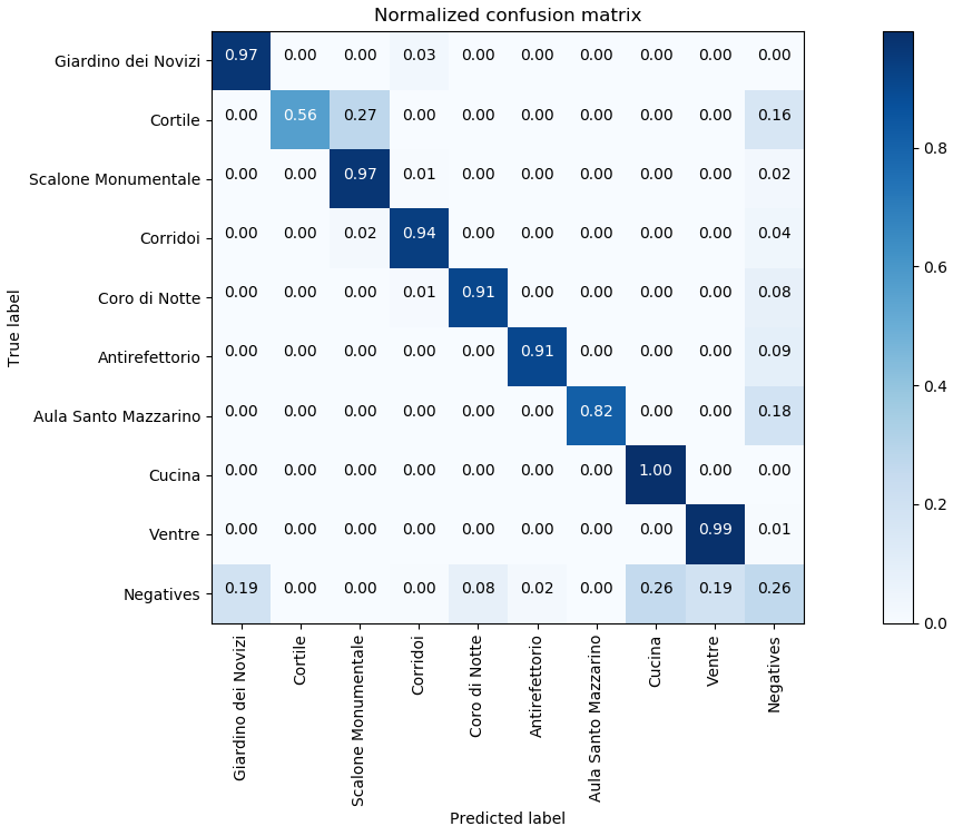
Figure 7. Confusion matrix of the results of the considered method on the GoPro test set.

Table 8 and Table 9 summarize and compare the results obtained training the algorithm on the two sets of data. Specifically, the tables report the average $FF_{1}$ and $ASF_{1}$ scores obtained in the three steps of the algorithm. As can be noted, significantly better discrimination is overall obtained using GoPro data ($0.88mFF_{1}$ vs $0.73mFF_{1}$). This is probably due to the wider Field Of View of the GoPro camera, which allows to capture more information about the surrounding environment (see Figure 2). Rejecting negative frames is a challenging task, which leads to degraded performances both in the case of frame-based measures (Table 8) and segment-based ones (Table 9). Interestingly, the negative rejection step works best on HoloLens data ($0.66mFF_{1}$ vs $0.54mFF_{1}$, and $0.24FF_{1}$ vs $0.18FF_{1}$ for the negative class). This result confirms the aforementioned observation that HoloLens data allows to acquire more distinctive details about the scene, thus allowing for more entropy when in the presence of unknown environments. The sequential modeling step, finally balances out the results, allowing HoloLens and GoPro to achieve similar performances.

Discrimination Rejection Seq. Modeling Class HoloLens GoPro HoloLens GoPro HoloLens GoPro 1 Cortile 0.50 0.84 0.45 0.25 0.59 0.57 2 Scalone Monumentale 0.81 0.93 0.84 0.91 0.96 0.95 3 Corridoi 0.77 0.92 0.69 0.83 0.92 0.97 4 Coro Di Notte 0.71 0.91 0.67 0.64 0.91 0.92 5 Antirefettorio 0.66 0.83 0.73 0.62 0.95 0.95 6 Aula Santo Mazzarino 0.69 0.81 0.65 0.23 0.99 0.90 7 Cucina 0.72 0.90 0.60 0.11 0.70 0.86 8 Ventre 0.97 0.99 0.94 0.86 0.96 0.88 9 Giardino dei Novizi 0.79 0.82 0.79 0.78 0.83 0.82 Negatives / / 0.24 0.18 0.42 0.30 $mFF_{1}$ 0.73 0.88 0.66 0.54 0.82 0.81

Table 8. Comparative table of average $FF_{1}$ scores for the considered method trained and tested on HoloLens and GoPro data. The table reports scores for the overall method (seq. modeling column), as well as for the two intermediate steps of Discrimination and Rejection.

Discrimination Rejection Seq. Modeling Class HoloLens GoPro HoloLens GoPro HoloLens GoPro 1 Cortile 0.01 0.15 0.02 0.03 0.48 0.68 2 Scalone Monumentale 0.01 0.05 0.01 0.03 0.90 0.85 3 Corridoi 0.00 0.02 0.00 0.01 0.79 0.88 4 Coro Di Notte 0.00 0.00 0.01 0.01 0.66 0.58 5 Antirefettorio 0.00 0.02 0.01 0.01 0.83 0.88 6 Aula Santo Mazzarino 0.00 0.00 0.00 0.00 0.96 0.81 7 Cucina 0.00 0.01 0.00 0.00 0.52 0.74 8 Ventre 0.00 0.32 0.00 0.03 0.92 0.66 9 Giardino dei Novizi 0.01 0.15 0.01 0.04 0.78 0.83 Negatives / / 0.01 0.00 0.27 0.23 $mASF_{1}$ 0.00 0.08 0.01 0.02 0.71 0.71

Table 9. Comparative table of average $AFF_{1}$ scores for the considered method trained and tested on HoloLens and GoPro data. The table reports scores for the overall method (seq. modeling column), as well as for the two intermediate steps of Discrimination and Rejection.

Figure 8 reports a qualitative comparison of the proposed method on ”Test3” video (acquired by HoloLens) and ”Test4” video (acquired by GoPro) used as validation videos. Please note that the two videos have been acquired simultaneously and so present similar content. The figure illustrates how the discrimination step allows to obtain more stable results in the case of GoPro data. For this reason, negative rejection tends to be more pronounced in the case of HoloLens data. The final segmentations obtained after the sequential modeling step are in general equivalent.

We would like to note that, even if the final results obtained using HoloLens and GoPro are equivalent in quantitative terms, the data acquired using the HoloLens device is deemed to carry more relevant information about what the user is actually looking at (see Figure 3). Such additional information can be leveraged in applications which go beyond localization, such as attention and behavioral modeling. Moreover, head-mounted devices such as HoloLens are better suited then chest-mounted cameras to provide additional services (e.g., augmented reality) to the visitor. This makes in our opinion HoloLens (and head-mounted devices in general) preferable. A series of demo videos to assess the performance of the investigated system are available at our web page http://iplab.dmi.unict.it/VEDI/video.html.

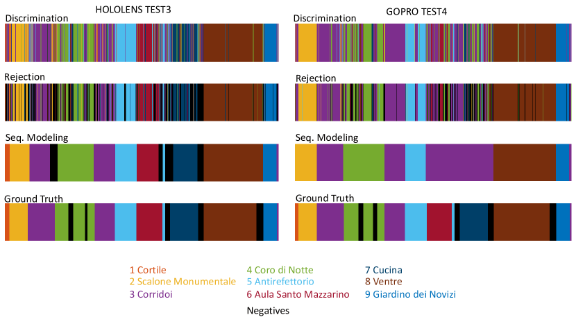
Figure 8. Color-coded segmentations for two corresponding test video acquired using HoloLens (left) and GoPro (right).

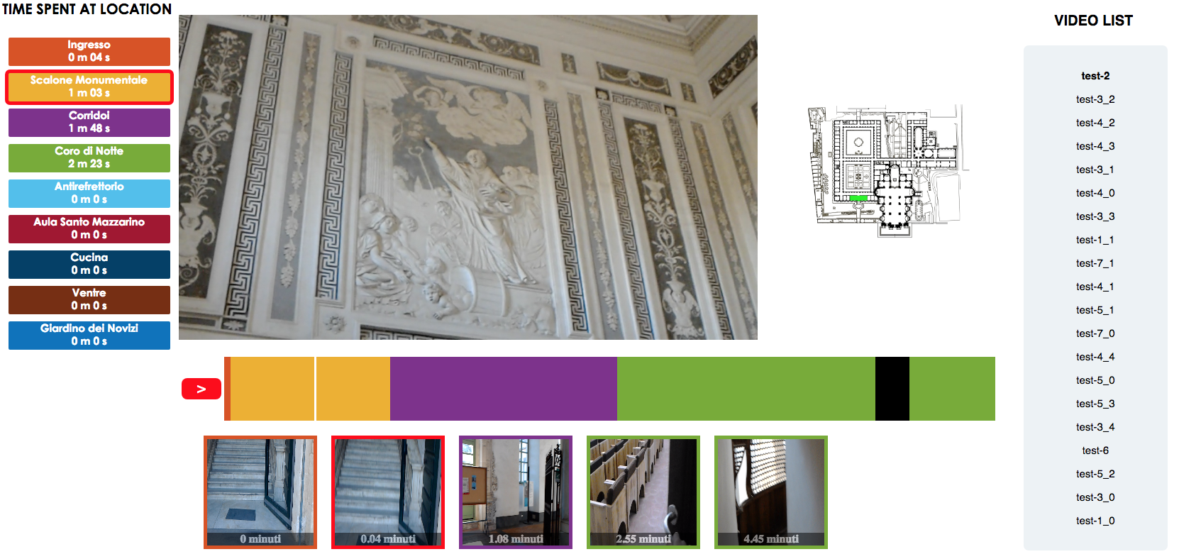
Figure 9. The GUI to allow the site manager to analyze the captured videos.

We also implemented a Manager Visualization Tool (MVT) as a web interface. The tool allows the manager to analyze the output of the system which automatically localizes the visitor in each frame of the video. The GUI allows the manager to select the video to be analyzed. A video player allows to skim through the video by clicking on a graphical representation of the inferred video segmentation. The GUI also presents the estimated time spent at each location and highlights the location of the visitor in a 2D map. Giving the opportunity to explore the video in a structured way, the system can provide useful information to the site manager. For instance, the site manager can infer which locations attract more the attention of the visitor, which can help improve the design of visit paths and profiling visitors. Figure 9 illustrates the different components of the developed tool. A video demo of the developed interface is available at http://iplab.dmi.unict.it/VEDI/demogui.html.

7. Conclusion

This work has investigated the problem of localizing visitors in a cultural site using egocentric (first person) cameras. To study the problem of room-level localization, we proposed and publicly released a dataset containing more than 4 hours of egocentric video, labeled according to the location of the visitor and to the observed cultural object of interest. The localization problem has been investigated reporting baseline results using a state-of-the-art method on data acquired using a head-mounted HoloLens and a chest-mounted GoPro device. Despite the larger field of view of the GoPro device, HoloLens allows to achieve similar performance in the localization task. We believe that the proposed UNICT-VEDI dataset will encourage further research on this domain. Future works will consider the problem of understanding which cultural objects are observed by the visitors. This will allow to provide more detailed information on the behavior and preferences of the visitors to the site manager. Moreover, the analysis will be extended and generalized to other cultural sites.

Supplementary Material

The dataset has been acquired using two devices (HoloLens and GoPro) and hence comprises two device-specifc training/testing sets. Video frames are labelled according to: 1) the environment of the visitor, 2) the point of interest he is looking at. Figure 2 reports some sample frames related to the different environments, whereas Figure 3 reports some sample frames related to the different points of interest. Table 10 summarizes the number of training videos acquired using HoloLens and GoPro devices. Table 11 summarizes the acquired test videos. In the following sections, we report additional material related to the data acquired using the HoloLens and GoPro devices.

Table 10. Summary of the collected training videos. On the left, we report the number of videos collected for the points of interest. On the right, we report the informations for the videos of collected for the environments. The values in the Time (s) and MB columns are related to the average time and occupied memory respectively.

	Points of interest			Environments
	# Videos	Time (s)	MB	# Videos	Time (s)	MB
Hololens	68	104	103	12	190	196
GoPro	68	93	233	12	186	455

Table 11. Summary of the acquired test videos . The values on the Time and MB columns are average values.

	Test Videos
	Number of videos	Time (s)	Storage (MB)
Hololens	7	780	730
GoPro	7	828	2062

Table 12. List of training videos of environments acquired using Hololens. For each video we show: time, amount of occupied memory, number of frames, percentage of frames with respect to the total number of frames of the training set.

Name	Time (s)	Storage (MB)	#frames	%frames
1.0_Cortile	48	48.145	1171	0,24%
2.0_Scalone	81	80.085	1947	0,40%
2.0_Scalone1	116	113.173	2747	0,56%
2.0_Scalone2	38	37.758	917	0,19%
4.0_CoroDiNotte	169	167.614	4068	0,83%
4.0_CoroDiNotte1	44	44.068	1067	0,22%
5.0_Antirefettorio	247	244.500	5933	1,21%
5.0_Antirefettorio1	263	260.395	6315	1,29%
6.0_SantoMazzarino	241	239.007	5800	1,18%
7.0_Cucina	239	237.268	5753	1,17%
8.0_Ventre	679	832.844	20385	4,15%
9.0_GiardinoNovizi	116	113.949	2788	0,57%
AVG	175.46	201.57	4908	1,00%

7.1. HoloLens

Table 12 details the training videos acquired to represent each of the considered environments. For each class, we report the total duration of the videos, the required storage, the number of frames and the percentage of frames, with respect to the total number of frames in the training set. Table LABEL:table:4 details the training videos acquired to represent each of the considered points of interest. For each class, we report the total duration of the videos, the required storage, the number of frames and the percentage of frames, with respect to the total number of frames in the training set. Table 14 reports a list of all test videos acquired using HoloLens. For each video, we report: Time, Storage, number of frames and percentage of frames with respect to the total number of frames of the training dataset.

Table 13. List of training videos of points of interest acquired with Hololens. For each video we show: Time, Storage, number of frames and percentage of frames with respect to the total number of frames of the training dataset. The table continues in the next page.

Name	Time (s)	Storage (MB)	#frame	%frame
2.1_Scalone_RampaS.Nicola	163	161.776	3926	0,80%
2.2_Scalone_RampaS.Benedetto	14	14.471	354	0,07%
2.2_Scalone_RampaS.Benedetto1	148	147.226	3573	0,73%
3.1_Corridoi_TreBiglie	75	74.261	1804	0,37%
3.2_Corridoi_ChiostroLevante	55	54.500	1328	0,27%
3.3_Corridoi_Plastico	80	79.179	1927	0,39%
3.4_Corridoi_Affresco	74	74.023	1800	0,37%
3.5_Corridoi_Finestra_ChiostroLev.	84	83.102	2035	0,41%
3.6_Corridoi_PortaCoroDiNotte	53	53.255	1291	0,26%
3.6_Corridoi_PortaCoroDiNotte1	60	59.411	1446	0,29%
3.6_Corridoi_PortaCoroDiNotte2	58	57.901	1406	0,29%
3.7_Corridoi_TracciaPortone	53	53.118	1291	0,26%
3.8_Corridoi_StanzaAbate	81	79.773	1948	0,40%
3.9_Corridoi_CorridoioDiLevante	89	88.173	2142	0,44%
3.10_Corridoi_CorridoioCorodiNotte	122	121.321	2945	0,60%
3.10_Corridoi_CorridoioCorodiNotte1	103	101.796	2472	0,50%
3.11_Corridoi_CorridoioOrologio	300	296.488	7202	1,47%
4.1_CoroDiNotte_Quadro	71	70.245	1716	0,35%
4.2_CoroDiNotte_Pav.Orig.Altare	73	72.358	1759	0,36%
4.3_CoroDiNotte_BalconeChiesa	39	39.331	957	0,19%
4.3_CoroDiNotte_BalconeChiesa1	49	48.550	1185	0,24%
4.3_CoroDiNotte_BalconeChiesa2	80	79.861	1935	0,39%
5.1_Antirefettorio_PortaA.S.Mazz.Ap.	67	67.001	1630	0,33%
5.1_Antirefettorio_PortaA.S.Mazz.Ch.	74	73.589	1785	0,36%
5.2_Antirefettorio_PortaMuseoFab.Ap.	50	49.840	1211	0,25%
5.2_Antirefettorio_PortaMuseoFab.Ch.	62	61.846	1503	0,31%
5.3_Antirefettorio_PortaAntiref.	51	58.557	1537	0,31%
5.4_Antirefettorio_PortaRef.Piccolo	54	53.767	1306	0,27%
5.5_Antirefettorio_Cupola	57	56.089	1377	0,28%
5.6_Antirefettorio_AperturaPavimento	55	54.586	1322	0,27%
5.7_Antirefettorio_S.Agata	48	47.820	1165	0,24%
5.8_Antirefettorio_S.Scolastica	58	57.919	1407	0,29%
5.9_Antirefettorio_ArcoconFirma	62	76.700	1864	0,38%
5.10_Antirefettorio_BustoVaccarini	65	64.298	1563	0,32%
6.1_SantoMazzarino_QuadroS.Mazz.	71	70.401	1716	0,35%
6.2_SantoMazzarino_Affresco	213	211.424	5124	1,04%
6.3_SantoMazzarino_PavimentoOr.	99	98.691	2397	0,49%
6.4_SantoMazzarino_PavimentoRes.	69	69.148	1675	0,34%
6.5_SantoMazzarino_BassorilieviManc.	117	115.348	2823	0,57%
6.6_SantoMazzarino_LavamaniSx	151	149.882	3637	0,74%
6.7_SantoMazzarino_LavamaniDx	93	92.928	2256	0,46%
6.8_SantoMazzarino_TavoloRelatori	150	148.661	3603	0,73%
6.9_SantoMazzarino_Poltrone	108	107.374	2604	0,53%
7.1_Cucina_Edicola	369	437.219	11086	2,26%
7.2_Cucina_PavimentoA	52	52.163	1268	0,26%
7.3_Cucina_PavimentoB	52	52.244	1266	0,26%
7.4_Cucina_PassavivandePavim.Orig.	81	80.733	1961	0,40%
7.5_Cucina_AperturaPav.1	57	57.170	1385	0,28%
7.5_Cucina_AperturaPav.2	53	52.875	1280	0,26%
7.5_Cucina_AperturaPav.3	62	62.320	1509	0,31%
7.6_Cucina_Scala	77	76.587	1856	0,38%
7.7_Cucina_SalaMetereologica	156	154.394	3748	0,76%
8.1_Ventre_Doccione	103	102.683	2492	0,51%
8.2_Ventre_VanoRacc.Cenere	126	124.837	3026	0,62%
8.3_Ventre_SalaRossa	300	296.792	7202	1,47%
8.4_Ventre_ScalaCucina	214	212.372	5152	1,05%
8.5_Ventre_CucinaProvv.	148	146.379	3553	0,72%
8.6_Ventre_Ghiacciaia	69	68.562	1668	0,34%
8.6_Ventre_Ghiacciaia1	266	263.817	6398	1,30%
8.7_Ventre_Latrina	102	100.542	2468	0,50%
8.8_Ventre_OssaScarti	154	152.861	3713	0,76%
8.8_Ventre_OssaScarti1	36	36.345	886	0,18%
8.9_Ventre_Pozzo	300	297.167	7209	1,47%
8.10_Ventre_Cisterna	57	56.572	1384	0,28%
8.11_Ventre_BustoP.Tacchini	110	109.520	2662	0,54%
9.1_GiardinoNovizi_NicchiaePav.	106	105.004	2555	0,52%
9.2_GiardinoNovizi_TraccePalestra	63	62.464	1525	0,31%
9.3_GiardinoNovizi_Pergolato	166	164.150	3984	0,81%
AVG	102.6	103.26	2517	0,51%

Table 14. List of test videos acquired using HoloLens. For each video we report the length in seconds, the amount of occupied memory, the number of frames, the number of environments included in the video, the number of points of interest included in the video, the sequence of environments as navigated by the visitor, and the sequence of points of interest, as navigated by the visitor.

Video	Time	MB	#frames	%frames	#env.	#p.int.	seq.environments	seq. p.interest
Test1	300	296.896	7202	5,49%	4	10	1->2->3->4	1.1->2.2->3.1->3.9->3.10->3.4-> 3.6->4.1->4.2->4.3
Test1.1	300	297.031	7202	5,49%	4	11	4->3->5->6	4.3->3.11->5.6->5.7->5.1->6.1-> 6.4->6.9->6.3->6.6->6.2
Test2.0	300	296.993	7203	5,49%	4	9	1_>2->3->4	1.1->2.1->3.9->3.10->3.5->3.10-> 3.5->3.10->3.6->4.1->4.2->4.3
Test3.0	300	296.959	7202	5,49%	4	8	1->2->3->4	1.1->2.1->3.9->3.10->3.4->3.11-> 3.6->4.1
Test3.1	300	296.913	7203	5,49%	3	5	4->3->5	4.2->4.3->4.2->3.11->5.5->5.6
Test3.2	300	297.083	7201	5,49%	4	17	5->6->5->7	5.6->5.1->5.3->5.10->5.9->5.1-> 6.2->6.1->6.4->6.9->6.5->6.4-> 6.3->6.8->6.5->6.7->6.6->6.5-> 5.2->7.1
Test3.3	300	297.160	7202	5,49%	2	12	7->8	7.2.>7.6->7.5->7.4->7.7->7.1-> 8.1->8.6->8.2->8.8->8.4->8.10
Test3.4	237	234.744	5694	4,34%	3	5	8->9->3	8.9->8.11->8.3->9.1->9.2
Test4.0	300	296.979	7204	5,49%	4	10	1->2->3->5	1.1->2.2->3.9->3.10->3.4->3.11-> ->3.7->3.11->5.10->5.9->5.1
Test4.1	300	296.654	7202	5,49%	3	16	5->7->8	5.6->5.5->5.8->5.4->5.2->7.1-> 7.3->7.2->7.1->7.4->7.1->7.5-> 7.7->7.1->8.1->8.5->8.2->8.4-> 8.7
Test4.2	136	135.143	3281	2,50%	1	3	8	8.10->8.9->8.11
Test4.3	300	296.853	7202	5,49%	4	7	8->9->3->4	8.3->9.1->9.3->9.2->3.11->3.6-> 4.2
Test4.4	201	199.585	4845	3,69%	3	4	4->3->2	4.2->3.10->3.9->2.1
Test5.0	274	271.524	6590	5,02%	4	11	1->2->3->2->3->4	1.1->3.1->3.3->3.2->2.1->3.9-> 3.10->3.5->3.10->3.5->3.10->3.4-> 3.7->3.4->3.6
Test5.1	300	296.801	7202	5,49%	4	11	4->3->9->3->5	4.1->4.2->3.6->3.11->9.2->3.11-> ->5.5->5.3->5.9->5.7->5.8->5.2
Test5.2	300	296.921	7202	5,49%	2	13	7->8	7.1->7.2->7.3->7.1->7.5->7.1-> 7.1->7.4->7.6->7.7->7.4->7.7-> 8.1->8.5->8.4->8.5->8.6->8.2-> 8.8->8.4
Test5.3	300	297.063	7201	5,49%	4	17	8->7->5->6	8.11->8.9->8.3->8.4->8.5->8.6-> 7.1->7.5->7.2->5.1->6.2->6.4-> 6.1->6.5->6.3->6.5->6.2->6.7-> 6.9
Test6.0	300	296.880	7202	5,49%	3	9	1->2->3	1.1->2.2->2.1->3.9->3.10->3.4-> 3.11->3.6->3.11->3.7->3.11
Test7.0	300	296.945	7202	5,49%	3	7	1->2->3	1.1->2.2->3.9->3.10->3.4->3.6-> 3.11
Test7.1	113	112.030	2721	2,07%	3	3	3->5->3	3.11->5.9->5.10->3.11

7.2. GoPro

Table 15 details the training videos acquired to represent each of the considered environments. For each class, we report the total duration of the videos, the required storage, the number of frames and the percentage of frames, with respect to the total number of frames in the training set. Table LABEL:table:5 details the training videos acquired to represent each of the considered points of interest. For each class, we report the total duration of the videos, the required storage, the number of frames and the percentage of frames, with respect to the total number of frames in the training set. Table 17 reports a list of all test videos acquired using GoPro. For each video, we report: Time, Storage, number of frames and percentage of frames with respect to the total number of frames of the training dataset.

Table 15. List of training videos of environments acquired using GoPro. For each video we show: time, amount of occupied memory, number of frames, percentage of frames with respect to the total number of frames of the training set.

Name	Time (s)	Storage (MB)	#frames	%frames
1.0_Cortile	47	116.798	1187	0,24%
2.0_Scalone	81	201.194	2044	0,42%
2.0_Scalone1	111	274.094	2785	0,57%
2.0_Scalone2	36	90.250	918	0,19%
4.0_CoroDiNotte	168	413.702	4205	0,86%
4.0_CoroDiNotte1	43	107.968	1097	0,22%
5.0_Antirefettorio	191	471.275	4790	0,97%
5.0_Antirefettorio1	262	644.852	6554	1,33%
6.0_SantoMazzarino	240	591.177	6009	1,22%
7.0_Cucina	241	592.907	6027	1,23%
8.0_Ventre	699	1719.352	17478	3,56%
9.0_GiardinoNovizi	116	427.472	6965	1,42%
AVG	186.25	242.62	5005	1,02%

Table 16. List of training videos of environments acquired using GoPro. For each video we show: time, amount of occupied memory, number of frames, percentage of frames with respect to the total number of frames of the training set.

Name	Time (s)	Storage (MB)	#frame	%frame
2.1_Scalone_RampaS.Nicola	160	394,844	4013	0,82%
2.2_Scalone_RampaS.Benedetto	14	35,758	363	0,07%
2.2_Scalone_RampaS.Benedetto1	147	361,856	3678	0,75%
3.1_Corridoi_TreBiglie	72	178,313	1812	0,37%
3.2_Corridoi_ChiostroLevante	54	202,165	3295	0,67%
3.3_Corridoi_Plastico	79	195,673	1989	0,40%
3.4_Corridoi_Affresco	74	182,106	1850	0,38%
3.5_Corridoi_Finestra_ChiostroLev.	81	300,474	4896	1,00%
3.6_Corridoi_PortaCoroDiNotte	50	123,34	1253	0,26%
3.6_Corridoi_PortaCoroDiNotte1	60	148,97	1514	0,31%
3.6_Corridoi_PortaCoroDiNotte2	58	142,747	1451	0,30%
3.7_Corridoi_TracciaPortone	55	136,484	1387	0,28%
3.8_Corridoi_StanzaAbate	58	122,859	1755	0,36%
3.9_Corridoi_CorridoioDiLevante	85	211,539	2148	0,44%
3.10_Corridoi_CorridoioCorodiNotte	120	297,325	3022	0,62%
3.10_Corridoi_CorridoioCorodiNotte1	100	246,769	2509	0,51%
3.11_Corridoi_CorridoioOrologio	176	434,081	4412	0,90%
4.1_CoroDiNotte_Quadro	69	171,551	1743	0,35%
4.2_CoroDiNotte_Pav.Orig.Altare	72	178,448	1813	0,37%
4.3_CoroDiNotte_BalconeChiesa	39	96,281	978	0,20%
4.3_CoroDiNotte_BalconeChiesa1	48	119,512	1214	0,25%
4.3_CoroDiNotte_BalconeChiesa2	80	197,29	2004	0,41%
5.1_Antirefettorio_PortaA.S.Mazz.Ap.	66	164,644	1673	0,34%
5.1_Antirefettorio_PortaA.S.Mazz.Ch	74	183,481	1864	0,38%
5.2_Antirefettorio_PortaMuseoFab.Ap	50	124,991	1270	0,26%
5.2_Antirefettorio_PortaMuseoFab.Ch	62	154,254	1567	0,32%
5.3_Antirefettorio_PortaAntiref.	52	128,695	1306	0,27%
5.4_Antirefettorio_PortaRef.Piccolo	54	133,494	1356	0,28%
5.5_Antirefettorio_Cupola	55	135,594	1378	0,28%
5.6_Antirefettorio_AperturaPavimento	57	141,647	1439	0,29%
5.7_Antirefettorio_S.Agata	49	120,611	1225	0,25%
5.8_Antirefettorio_S.Scolastica	56	137,79	1400	0,28%
5.9_Antirefettorio_ArcoconFirma	60	149,889	1522	0,31%
5.10_Antirefettorio_BustoVaccarini	66	162,799	1654	0,34%
6.1_SantoMazzarino_QuadroS.Mazz.	72	178,16	1810	0,37%
6.2_SantoMazzarino_Affresco	214	526,612	5353	1,09%
6.3_SantoMazzarino_PavimentoOr.	98	242,332	2462	0,50%
6.4_SantoMazzarino_PavimentoRes.	68	169,524	1722	0,35%
6.5_SantoMazzarino_BassorilieviMan.	116	25,942	2906	0,59%
6.6_SantoMazzarino_LavamaniSx	134	331,517	3369	0,69%
6.7_SantoMazzarino_LavamaniDx	91	225,892	2296	0,47%
6.8_SantoMazzarino_TavoloRelatori	149	366,575	3726	0,76%
6.9_SantoMazzarino_Poltrone	108	266,611	2709	0,55%
7.1_Cucina_Edicola	368	931,368	9467	1,93%
7.2_Cucina_PavimentoA	55	137,197	1394	0,28%
7.3_Cucina_PavimentoB	52	129,601	1316	0,27%
7.4_Cucina_PassavivandePavim.Orig.	84	206,667	2100	0,43%
7.5_Cucina_AperturaPav.1	58	142,7	1450	0,30%
7.5_Cucina_AperturaPav.2	57	142,145	1444	0,29%
7.5_Cucina_AperturaPav.3	65	161,61	1641	0,33%
7.6_Cucina_Scala	79	195,547	1988	0,40%
7.7_Cucina_SalaMetereologica	158	390,583	3970	0,81%
8.1_Ventre_Doccione	100	246,353	2503	0,51%
8.2_Ventre_VanoRacc.Cenere	128	315,824	3210	0,65%
8.3_Ventre_SalaRossa	158	388,603	3951	0,80%
8.4_Ventre_ScalaCucina	213	524,06	5327	1,08%
8.5_Ventre_CucinaProvv.	151	371,84	3779	0,77%
8.6_Ventre_Ghiacciaia	72	178,295	1811	0,37%
8.6_Ventre_Ghiacciaia1	185	457,1	4646	0,95%
8.7_Ventre_Latrina	80	295,294	4804	0,98%
8.8_Ventre_OssaScarti	150	369,523	3756	0,76%
8.8_Ventre_OssaScarti1	34	86,105	873	0,18%
8.9_Ventre_Pozzo	149	367,713	3737	0,76%
8.10_Ventre_Cisterna	30	114,114	1852	0,38%
8.11_Ventre_BustoP.Tacchini	106	261,822	2661	0,54%
9.1_GiardinoNovizi_NicchiaePav.	104	256,731	2609	0,53%
9.2_GiardinoNovizi_TraccePalestra	58	216,801	3533	0,72%
9.3_GiardinoNovizi_Pergolato	164	404,893	4115	0,84%
AVG	93.53	232.97	2515	0,51%

Table 17. List of test videos acquired using GoPro. For each video we report the length in seconds, the amount of occupied memory, the number of frames, the number of environments included in the video, the number of points of interest included in the video, the sequence of environments as navigated by the visitor, and the sequence of points of interest, as navigated by the visitor.

Video	Time(s)	MB	#frames	%frames	#env.	#p.int.	sequence environements	sequence points of interest
Test1	397	390.558	14788	5.32%	4	9	1.0->2.0->3.0->4.0->3.0	1.1->2.2->3.9->3.10->3.6->4.1-> 4.2->4.3->3.11
Test2	420	1033.149	10503	3.78%	4	8	1.0->2.0->3.0->5.0->3.0	1.1->2.1->3.9->3.10->3.4->3.11-> 3.6->3.11->5.10->3.10
Test3	579	1425.480	14491	5.21%	5	11	1.0->2.0->3.0->9.0->3.0->5.0->3.0	1.1->2.2->2.1->2.2->3.9->3.10-> 3.6->3.11->9.2->9.1->9.3->9.2-> 3.11->5.10->3.11
Test4	1472	3620.627	36808	13.24%	9	35	1.0->2.0->3.0->4.0->3.0->5.0-> 6.0->5.0->7.0->8.0->9.0->3.0	1.1->2.1->2.2->3.9->3.10->3.4-> 3.11->3.6->4.1->4.3->3.11->5.4-> 5.2->5.1->5.3->5.10->5.9->5.6->5.1-> 6.9->6.4->6.9->6.8->5.3->5.6-> 5.4->5.2->7.1->7.6->7.1->7.5-> 7.4->7.7->8.1->8.6->8.2->8.8-> 8.1->8.10->8.9->8.11->8.3->9.1->9.2
Test5	751	1848.142	18788	6.76%	6	26	1.0->2.0->3.0->5.0->7.0->8.0	1.1->2.2->2.1->3.1->3.9->3.10-> 3.4->3.11->5.10->5.6->5.1->5.3-> 5.4->5.2->7.1->7.4->7.1->7.5-> 7.7->8.1->8.5->8.4->8.7->8.10-> 8.8->8.10->8.11
Test6	506	1245.254	12661	4.56%	5	11	8.0->9.0->3.0->4.0->3.0->2.0	8.3->9.1->9.3->9.2->3.11->3.6-> 4.2->3.10->3.9->3.1->2.1
Test7	1549	3809.218	38725	13.93%	9	44	1.0->2.0->3.0->2.0->3.0->4.0-> 3.0->9.0->3.0->5.0->7.0->8.0-> 7.0->5.0->6.0->5.0->3.0->9.0-> 3.0->2.0->1.0	1.1->2.1->3.3->3.2->2.1->3.9-> 3.10->3.5->3.10->3.5->3.10->3.4-> 3.11->3.7->3.11->3.10->3.4->3.6-> 4.1->4.3->3.6->3.11->9.2->9.1-> 9.2->3.11->5.7->5.4->5.3->5.2-> 7.1->7.5->7.4->7.6->7.1->7.7-> 7.4->7.7->8.1->8.5->8.4->8.6-> 8.2->8.8->8.4->8.10->8.11->8.3-> 8.5->7.1->6.2->6.1->6.5->6.9-> 6.6->6.5->6.8->6.4->5.3->5.10-> 3.11->9.1->9.3->9.2->3.11->3.10-> 3.5->3.10->3.9->2.1->2.2->1.1

References

- (1)
- Amato et al. (2015) Giuseppe Amato, Fabrizio Falchi, and Claudio Gennaro. 2015. Fast image classification for monument recognition. Journal on Computing and Cultural Heritage (JOCCH) 8, 4 (2015), 18.
- Aoki et al. (1998) Hisashi Aoki, Bernt Schiele, and Alex Pentland. 1998. Recognizing personal location from video. In Workshop on Perceptual User Interfaces. ACM, 79–82.
- Bartoli et al. (2015) Federico Bartoli, Giuseppe Lisanti, Lorenzo Seidenari, Svebor Karaman, and Alberto Del Bimbo. 2015. Museumvisitors: a dataset for pedestrian and group detection, gaze estimation and behavior understanding. In Proceedings of the IEEE Conference on Computer Vision and Pattern Recognition Workshops. 19–27.
- Bishop (2006) C. M. Bishop. 2006. Pattern recognition and Machine Learning. Springer.
- Colace et al. (2014) Francesco Colace, Massimo De Santo, Luca Greco, Saverio Lemma, Marco Lombardi, Vincenzo Moscato, and Antonio Picariello. 2014. A Context-Aware Framework for Cultural Heritage Applications. In Signal-Image Technology and Internet-Based Systems (SITIS), 2014 Tenth International Conference on. IEEE, 469–476.
- Cucchiara and Del Bimbo (2014) Rita Cucchiara and Alberto Del Bimbo. 2014. Visions for augmented cultural heritage experience. IEEE MultiMedia 21, 1 (2014), 74–82.
- Curran et al. (2011) Kevin Curran, Eoghan Furey, Tom Lunney, Jose Santos, Derek Woods, and Aiden McCaughey. 2011. An evaluation of indoor location determination technologies. Journal of Location Based Services 5, 2 (2011), 61–78.
- Furnari et al. (2018) Antonino Furnari, Sebastiano Battiato, and Giovanni Maria Farinella. 2018. Personal-Location-Based Temporal Segmentation of Egocentric Video for Lifelogging Applications. Journal of Visual Communication and Image Representation (2018). https://doi.org/10.1016/j.jvcir.2018.01.019
- Gallo et al. (2017) G Gallo, G Signorello, GM Farinella, and A Torrisi. 2017. Exploiting Social Images to Understand Tourist Behaviour. In International Conference on Image Analysis and Processing, Vol. LNCS 10485. Springer, 707–717.
- Gu et al. (2009) Yanying Gu, Anthony Lo, and Ignas Niemegeers. 2009. A survey of indoor positioning systems for wireless personal networks. IEEE Communications surveys & tutorials 11, 1 (2009), 13–32.
- Ishihara et al. (2017a) Tatsuya Ishihara, Kris M Kitani, Chieko Asakawa, and Michitaka Hirose. 2017a. Inference Machines for supervised Bluetooth localization. In Acoustics, Speech and Signal Processing (ICASSP), 2017 IEEE International Conference on. 5950–5954.
- Ishihara et al. (2017b) Tatsuya Ishihara, Jayakorn Vongkulbhisal, Kris M Kitani, and Chieko Asakawa. 2017b. Beacon-Guided Structure from Motion for Smartphone-Based Navigation. In Applications of Computer Vision (WACV), 2017 IEEE Winter Conference on. 769–777.
- Jia et al. (2014) Yangqing Jia, Evan Shelhamer, Jeff Donahue, Sergey Karayev, Jonathan Long, Ross Girshick, Sergio Guadarrama, and Trevor Darrell. 2014. Caffe: Convolutional architecture for fast feature embedding. In Proceedings of the 22nd ACM international conference on Multimedia. ACM, 675–678.
- Kendall et al. (2015) Alex Kendall, Matthew Grimes, and Roberto Cipolla. 2015. Posenet: A convolutional network for real-time 6-dof camera relocalization. In Proceedings of the IEEE international conference on computer vision. 2938–2946.
- Li et al. (2017) Qing Li, Jiasong Zhu, Tao Liu, Jon Garibaldi, Qingquan Li, and Guoping Qiu. 2017. Visual landmark sequence-based indoor localization. In Proceedings of the 1st Workshop on Artificial Intelligence and Deep Learning for Geographic Knowledge Discovery. 14–23.
- Oliva and Torralba (2001) Aude Oliva and Antonio Torralba. 2001. Modeling the shape of the scene: A holistic representation of the spatial envelope. International journal of computer vision 42, 3 (2001), 145–175.
- Portaz et al. (2017a) Maxime Portaz, Matthias Kohl, Georges Quénot, and Jean-Pierre Chevallet. 2017a. Fully Convolutional Network and Region Proposal for Instance Identification with egocentric vision. In Proceedings of the IEEE Conference on Computer Vision and Pattern Recognition. 2383–2391.
- Portaz et al. (2017b) Maxime Portaz, Johann Poignant, Mateusz Budnik, Philippe Mulhem, Jean-Pierre Chevallet, and Lorraine Goeuriot. 2017b. Construction et évaluation d’un corpus pour la recherche d’instances d’images muséales.. In CORIA. 17–34.
- Sattler et al. (2017) Torsten Sattler, Bastian Leibe, and Leif Kobbelt. 2017. Efficient & effective prioritized matching for large-scale image-based localization. IEEE transactions on pattern analysis and machine intelligence 39, 9 (2017), 1744–1756.
- Seidenari et al. (2017) Lorenzo Seidenari, Claudio Baecchi, Tiberio Uricchio, Andrea Ferracani, Marco Bertini, and Alberto Del Bimbo. 2017. Deep Artwork Detection and Retrieval for Automatic Context-Aware Audio Guides. ACM Transactions on Multimedia Computing, Communications, and Applications (TOMM) 13, 3s (2017), 35.
- Shotton et al. (2013) Jamie Shotton, Ben Glocker, Christopher Zach, Shahram Izadi, Antonio Criminisi, and Andrew Fitzgibbon. 2013. Scene coordinate regression forests for camera relocalization in RGB-D images. In Proceedings of the IEEE Conference on Computer Vision and Pattern Recognition. 2930–2937.
- Signorello et al. (2015) Giovanni Signorello, Giovanni Maria Farinella, Giovanni Gallo, Luciano Santo, Antonino Lopes, and Emanuele Scuderi. 2015. Exploring Protected Nature Through Multimodal Navigation of Multimedia Contents. In International Conference on Advanced Concepts for Intelligent Vision Systems. 841–852.
- Simonyan and Zisserman (2014) K. Simonyan and A. Zisserman. 2014. Very Deep Convolutional Networks for Large-Scale Image Recognition. CoRR abs/1409.1556 (2014).
- Starner et al. (1998) T. Starner, B. Schiele, and A. Pentland. 1998. Visual contextual awareness in wearable computing. In International Symposium on Wearable Computing. 50–57.
- Taverriti et al. (2016) Giovanni Taverriti, Stefano Lombini, Lorenzo Seidenari, Marco Bertini, and Alberto Del Bimbo. 2016. Real-time Wearable Computer Vision System for Improved Museum Experience. In Proceedings of the 2016 ACM on Multimedia Conference. ACM, 703–704.
- Torralba et al. (2003) Antonio Torralba, Kevin P Murphy, William T Freeman, and Mark A Rubin. 2003. Context-based vision system for place and object recognition. In Computer Vision, 2003. Proceedings. Ninth IEEE International Conference on. IEEE, 273–280.
- Want and Hopper (1992) Roy Want and Andy Hopper. 1992. Active badges and personal interactive computing objects. IEEE Transactions on Consumer Electronics 38, 1 (1992), 10–20.
- Weyand and Leibe (2015) Tobias Weyand and Bastian Leibe. 2015. Visual landmark recognition from Internet photo collections: A large-scale evaluation. Computer Vision and Image Understanding 135 (2015), 1 – 15. https://doi.org/10.1016/j.cviu.2015.02.002
- Xu et al. (2014) Qianli Xu, Liyuan Li, Joo Hwee Lim, Cheston Yin Chet Tan, Michal Mukawa, and Gang Wang. 2014. A wearable virtual guide for context-aware cognitive indoor navigation. In Proceedings of the 16th international conference on Human-computer interaction with mobile devices & services. ACM, 111–120.
- Zhou et al. (2014) B. Zhou, A. Lapedriza, J. Xiao, A. Torralba, and A. Oliva. 2014. Learning deep features for scene recognition using places database. In Advances in Neural Information Processing Systems. 487–495.