Two-photon Rabi-Hubbard and Jaynes-Cummings-Hubbard models: photon pair superradiance, Mott insulator and normal phases

Abstract

We study the ground state phase diagrams of two-photon Dicke, the one-dimensional Jaynes-Cummings-Hubbard (JCH), and Rabi-Hubbard (RH) models using mean field, perturbation, quantum Monte Carlo (QMC), and density matrix renormalization group (DMRG) methods. We first compare mean field predictions for the phase diagram of the Dicke model with exact QMC results and find excellent agreement. The phase diagram of the JCH model is then shown to exhibit a single Mott insulator lobe with two excitons per site, a superfluid (SF, superradiant) phase and a large region of instability where the Hamiltonian becomes unbounded. Unlike the one-photon model, there are no higher Mott lobes. Also unlike the one-photon case, the SF phases above and below the Mott are surprisingly different: Below the Mott, the SF is that of photon pairs as opposed to above the Mott where it is SF of simple photons. The mean field phase diagram of the RH model predicts a transition from a normal to a superradiant phase but none is found with QMC.

I Introduction

Continued progress in controlling and tuning interactions between photons and individual atoms has made possible the realization of elementary quantum electrodynamics building blocksschoelkopf08 using two-level atoms in cavitiesharoche06 or Josephson junctions on solid state chipswallraff04 ; chen07 ; lambert09 ; nataf10 ; viehmann11 (circuit QED). Generally speaking, such couplings of photons to two-level systems are well described by the Rabi modelrabi36 ; rabi37 . In what is referred to as the strong coupling limit, $g/\omega\lesssim 0.1$, (see below) one can apply the random wave approximation (RWA) and ignore “counter rotating” (CR) terms which do not conserve the number of excitons (the number of photons plus the number of excited atoms). When these terms are ignored, we obtain the Jaynes-Cummings modeljaynes63 which, due its $U(1)$ symmetry, conserves the number of excitons and can be solved exactly for a single cavity. An ensemble of such cavities can be connected (here we consider a one-dimensional chain) by tuning the tunneling rate of the photon modes between near neighbor cavities resulting in a lattice model, the Jaynes-Cummings-Hubbard model, which consists of itinerant bosons (photons) hopping between near neighbor sites and interacting with localized two-level atoms (“spins” or qubits). The properties of this model were shown to be very similar to those of the one-dimensional Bose-Hubbard model (BHM)batrouni90 exhibiting a superfluid phase (of excitons) and incompressible Mott insulator (MI) lobesgreentree06 ; hartmann06 ; rossini07 ; koch08 ; hohenadler08 ; hartmann08 ; schmidt09 ; zhao08 . The MI is essentially a product single site states composed of a superposition of photons and excited atomsschmidt09 and exhibits behavior similar to photon blockadebirnbaum05 where there is a finite energy gap opposing the addition of a photon. Long range frustrated hoppinghohenadler12 and dynamic properties of this model have also elicited much interestpippan09 ; tomadin10 ; tomadin10b ; hohenadler11 ; carusotto13 . When the coupling becomes of the order of the photon frequency, $g/\omega$, the “ultra-strong coupling” regime which has been achieved experimentallyniemczyk10 ; forndiaz10 ; chen17 ; forndiaz17 ; yoshihara17 , the RWA is no longer valid and the counter rotating terms come into play reducing the symmetry from $U(1)$ to $Z_{2}$. This has several consequences: (a) CR terms cause the exciton number not to be conserved thus excluding the possibility of any Mott phases, (b) the system is now in the universality class of the Ising model with two phases, a disordered and an ordered (coherent) phase, (c) due to the discrete nature of the symmetry, it can break spontaneously in one dimension. Consequently, the ordered coherent phase is a photon Bose-Einstein condensate (BEC) and the transition between this phase and the disordered phase exhibits Ising critical exponentsschiro13 ; zheng11 ; schiro13 ; kumar13 ; flottat16 . This transition resembles the incoherent/coherent (normal/superradiant) phase transition in the Dicke modelhepp73 ; rotondo15 .

Multi-photon processes have also attracted scrutiny as more experimental systems are being realized where such physics enters into play. For example, the two-photon Rabi model has been used as an effective model to describe second order processes in Rydberg atoms in cavitiesbertet02 and quantum dotsstufler06 ; delvalle10 , and mechanisms have been proposed to realize it in circuit QEDfelicetti18 . Unlike the one-photon case, the two-photon Rabi model undergoes spectral collapse, where the Hamiltonian is no longer bounded from below, when the coupling exceeds a certain valueemary02 ; dolya09 ; travenec12 ; maciejewski15 ; travenec15 ; peng17 ; chen12 ; felicetti15 . As in the one-photon case, in the strong coupling limit where the CR terms can be ignored, the Hamiltonian has $U(1)$ symmetry. In the ultra strong coupling limit, where the CR terms must be restored, the symmetry is reduced to $Z_{2n}$ for the $n$-photon case, i.e. $Z_{4}$ in the two-photon case. The ground state of the many-body two-photon model was studied in the context of the Dicke modeldicke54 using mean field methodsgarbe17 . A quantum phase transition between a normal (disordered) and superradiant phase was predicted. In this model, however, the term superradiant is used to indicate a macroscopic change in the average number of photons but which remains relatively small. This is to be contrasted with the one-photon case where there is a very large number of photons in the superradiant phase and they form a BECschiro13 ; zheng11 ; schiro13 ; kumar13 ; flottat16 . The spectral collapse region was also found.

In this paper we will first use exact QMC simulations to determine the phase diagram of the two-photon Dicke model and compare with mean field resultsgarbe17 . This also serves to verify our QMC method. We then use our QMC algorithm, and also DMRG calculations, to study the phase diagram of another many-body system, namely the one-dimensional two-photon Jaynes-Cummings-Hubbard (JCH) model. The numerical results are compared with perturbation and mean field calculations. Finally, we use our numerical methods to study the full Rabi-Hubbard model.

Our results below show that the mean field phase diagram of the Dicke model is in agreement with our exact QMC simulations. In addition, we find that, surprisingly, the Jaynes-Cummings-Hubbard model exhibits only one Mott insulating lobe before the systems becomes unstable. Furthermore, doping above the MI yields a photon superfluid phase, while doping below the MI yields an unexpected photon pair superfluid phase. QMC simulations suggest that the Rabi-Hubbard model does not exhibit a phase transition from a normal to a superradiant phase.

The paper is organized as follows. In section II we describe the models and the physical quantities we will study. In section III we review the mean field calculation for the Dicke model and discuss our exact QMC results. In section IV we show our perturbation and exact QMC results for the JCH model followed by section V where we discuss the RH model. We present some conclusions in section VI followed by appendices A, B, and C where we show details of some of our calculations.

II Models

We will first study the two-photon Dicke model where $N$ two-level systems (qubits) couple to a single photon mode and which is governed by the Hamiltonian

$$H_{D} = \omega{\hat{a}}^{\dagger}{\hat{a}}^{\phantom{\dagger}}+\frac{\omega_{q}}{2}\sum_{j=1}^{N}\sigma^{z}_{j}+\frac{g}{N}\sum_{j=1}^{N}\sigma^{x}_{j}({\hat{a}}^{2}+{\hat{a}}^{\dagger 2})$$ (1)

$$= \omega{\hat{a}}^{\dagger}{\hat{a}}^{\phantom{\dagger}}+\frac{\omega_{q}}{2}\sum_{j=1}^{N}\sigma^{z}_{j}$$

$$+\frac{g}{N}\sum_{j=1}^{N}(\sigma^{+}_{j}+\sigma^{-}_{j})({\hat{a}}^{2}+{\hat{a}}^{\dagger 2}).$$

This model was examined with mean field in Ref. garbe17, . Here, $\omega$ is the photon frequency, $\omega_{q}$ the qubit energy spacing, $g$ the coupling constant, $\hat{a}$ (${\hat{a}}^{\dagger}$) is the photon destruction (creation) operator, $\sigma^{z}_{i}$ and $\sigma^{x}_{j}=\sigma^{+}_{j}+\sigma^{-}_{j}$ are Pauli matrices acting on the $j$th qubit, $\sigma^{+}_{j}$ ($\sigma^{-}_{j}$) is the corresponding raising (lowering) operator. A related model is the Rabi-Hubbard (RH) model,

$$H_{RH} = -J\sum_{i=1}^{N}\left({\hat{a}}^{\dagger}_{i}{\hat{a}}^{\phantom{\dagger}}_{i+1}+h.c.\right)+\sum_{i=1}^{N}\left(\omega{\hat{a}}^{\dagger}_{i}{\hat{a}}^{\phantom{\dagger}}_{i}+\omega_{q}\sigma^{+}_{i}\sigma^{-}_{i}\right)$$ (2)

$$+g\sum_{i=1}^{N}\left(\sigma^{+}_{i}+\sigma^{-}_{i}\right)\left({\hat{a}}^{2}_{i}+{\hat{a}}^{\dagger 2}_{i}\right),$$

where now $N$ is the number of sites (or cavities) and ${\hat{a}}_{i}$ is the photon mode in the $i$th cavity. Note that photon modes can tunnel between sites. Ignoring in Eq. (2) the CR terms, $(\sigma^{+}_{i}{\hat{a}}^{\dagger 2}_{i}+\sigma^{-}_{i}{\hat{a}}^{2}_{i}$), yields the Jaynes-Cummings-Hubbard (JCH) model in which the number of excitons is conserved.

In both models, Eq. (1) and Eq. (2), when the CR terms are dropped, the system is invariant under the generalized rotation operator,

$${\cal R}(\theta)={\rm exp}\left(i\theta{\hat{a}}^{\dagger}_{j}{\hat{a}}^{\phantom{\dagger}}_{j}+i2\theta\sigma^{+}_{j}\sigma^{-}_{j}\right),$$ (3)

with ${\cal R}(\theta)^{\dagger}{\hat{a}}_{j}{\cal R}(\theta)^{\phantom{\dagger}}={\rm e}^{i\theta}{\hat{a}}_{j}$, and ${\cal R}(\theta)^{\dagger}\sigma^{-}_{j}{\cal R}(\theta)^{\phantom{\dagger}}={\rm e}^{i2\theta}\sigma^{-}_{j}$ for any $\theta$, thus exhibiting $U(1)$ symmetry. However, the action of ${\cal R}(\theta)$ on the CR terms introduces a phase ${\rm exp}(i4\theta)$ thus reducing the symmetry to $Z_{4}$, in other words, the system is left invariant by the rotation only for $\theta=n2\pi/4$, $n=0,1,2,3$. Therefore, when the CR terms are ignored, the $U(1)$ symmetry results in the conservation of the number of excitons, $N_{exc}=N_{photon}+2N_{+}$ where $N_{+}$ is the number of qubits in the excited state. De-exciting a qubit generates two photons and vice versa. On the other hand, in the presence of the CR terms, $N_{exc}$ is not conserved, and quantum phase transitions would be expected to reflect the discrete $Z_{4}$ symmetry. Note that this discrete symmetry can break spontaneously for a one-dimensional quantum system in its ground state.

To characterize the various possible phases, we calculate several Green functions,

$$G_{\alpha,\beta}(r)\equiv\frac{1}{2N}\sum_{i}\langle\alpha_{i}\beta_{i+r}+{\rm h.c.}\rangle,$$ (4)

where $\alpha$ and $\beta$ denote creation and annihilation operators of the photons (${\hat{a}}^{\dagger}_{i}$ and ${\hat{a}}^{\phantom{\dagger}}_{i}$) or the qubits ($\sigma^{+}_{j}$ and $\sigma^{-}_{j}$). For example, the photon Green function at equal time is given by,

$$G_{a^{\dagger},a^{\phantom{\dagger}}}(r)=\frac{1}{2N}\sum_{i}\langle{\hat{a}}^{\dagger}_{i}{\hat{a}}^{\phantom{\dagger}}_{i+r}+{\hat{a}}^{\dagger}_{i+r}{\hat{a}}^{\phantom{\dagger}}_{i}\rangle.$$ (5)

The qubit Green function is,

$$G_{\sigma^{-},\sigma^{+}}(r)=\frac{1}{2N}\sum_{i}\langle\sigma^{-}_{i}\sigma^{+}_{i+r}+\sigma^{-}_{i+r}\sigma^{+}_{i}\rangle,$$ (6)

and the following two functions will be particularly useful:

$$G_{\sigma^{+},a}(r)=\frac{1}{2N}\sum_{i}\langle{\hat{a}}^{\phantom{\dagger}}_{i}\sigma^{+}_{i+r}+\sigma^{-}_{i+r}{\hat{a}}^{\dagger}_{i}\rangle,$$ (7)

and

$$G_{\sigma^{+},a^{2}}(r)=\frac{1}{2N}\sum_{i}\langle{\hat{a}}^{2}_{i}\sigma^{+}_{i+r}+\sigma^{-}_{i+r}{\hat{a}}^{\dagger 2}_{i}\rangle.$$ (8)

Power law decay of one of these Green functions would indicate quasi-long range order for the corresponding quantity. We also measure the average number of excitons,

$$N_{exc}=\sum_{i}\langle{\hat{a}}^{\dagger}_{i}{\hat{a}}^{\phantom{\dagger}}_{i}+2\sigma_{i}^{+}\sigma_{i}^{-}\rangle,$$ (9)

and the superfluid density,

$$\rho_{s}=\frac{\langle W^{2}\rangle}{2t\beta L^{d-2}},$$ (10)

where $W$ is the winding number of an exciton and $d$ the dimensionality. To study the phase diagrams of these models, we use several methods: Mean field, perturbation expansion, QMC and DMRG.

III The Dicke Model

First, we will review briefly the mean field results of Ref. garbe17, and then discuss our QMC results. First the total angular momentum operators are defined, ${\hat{J}}_{z}\equiv\sum_{i}\sigma^{z}_{i}/2$ and ${\hat{J}}^{\pm}\equiv\sum_{i}\sigma^{\pm}_{i}$. Then using the Holstein-Primakoff (HP) transformation, they define the bosonic operators:

$${\hat{J}}^{+}={\hat{b}}^{\dagger}\sqrt{N-{\hat{b}}^{\dagger}{\hat{b}}^{\phantom{\dagger}}},\,\,\,{\hat{J}}^{-}=\sqrt{N-{\hat{b}}^{\dagger}{\hat{b}}^{\phantom{\dagger}}}\,{\hat{b}}^{\phantom{\dagger}},\,\,\,{\hat{J}}_{z}={\hat{b}}^{\dagger}{\hat{b}}^{\phantom{\dagger}}-\frac{N}{2},$$ (11)

where $[{\hat{b}},{\hat{b}}^{\dagger}]=1$. Then the bosonic operators are replaced by the average value in the ground state, ${\hat{b}}\to{\bar{b}}=\langle GS|{\hat{b}}|GS\rangle$. Making the substitutions in the Hamiltonian, Eq. (1), yields,

$$H^{MF}_{D}=\omega{\hat{a}}^{\dagger}{\hat{a}}+g_{\bar{b}}({\hat{a}}^{2}+{\hat{a}}^{\dagger 2})+\omega_{q}|{\bar{b}}|^{2}-\frac{\omega_{q}N}{2},$$ (12)

with

$$g_{\bar{b}}=\frac{g}{N}({\bar{b}}+{\bar{b}}^{*})\sqrt{N-|{\bar{b}}|^{2}}.$$ (13)

The Hamiltonian is now a quadratic in the photon operators and can be diagonalized exactly giving the ground state energy, $E_{G}$, which is to be minimized with respect to ${\bar{b}}$. This determines the value of the order parameter, ${\bar{b}}$ as a function of the other parameters $\omega$, $\omega_{q}$ and $g$. It was found that for $g<g_{c}=\sqrt{\omega\omega_{q}N/4}$, $E_{G}$ is minimum for ${\bar{b}}={\bar{b}}^{*}=0$. For $g>g_{c}$, the ground state is twofold degenerate and the order parameter, acquires a nonzero value, ${\bar{b}}={\bar{b}}^{*}$:

$${\bar{b}} = \pm\sqrt{\frac{N}{2}}\left(1-\sqrt{\frac{1-\mu}{4\mu^{2}\lambda^{2}-\mu}}\right)^{1/2}$$ (14)

$$\lambda = \frac{\omega}{2\omega_{q}N}\geq 0$$ (15)

$$\mu = \frac{4g^{2}}{\omega^{2}}.$$ (16)

Therefore, the system exhibits two phases, a normal phase (${\bar{b}}=0$) and a superradiant phase (${\bar{b}}\neq 0$) separated by the transition line $g_{c}=\sqrt{\omega\omega_{q}N/4}$. Furthermore, for $g>\omega/2$, the argument of the square root in Eq. (14) becomes negative indicating that the Hamiltonian is unbounded. These results map out the phase diagram as shown in Ref. garbe17, .

It is interesting to examine the accuracy of mean field calculations in various situations. We therefore performed QMC simulations using the stochastic Green function (SGF) methodrousseau08 ; rousseau08b , both to verify our QMC simulations and obtain the numerically exact ground state phase diagram. To map out the phase diagram, we choose $\omega=1$ to set the energy scale, and we calculate the order parameter for many values of $g$ at fixed $N\omega_{q}$. Making several such cuts for different $N\omega_{q}$ yields the phase diagram in the $(N\omega_{q},g)$ plane. In the mean field calculation, the order parameter was ${\bar{b}}=\langle GS|b|GS\rangle$; in the QMC simulations, we take the order parameter to be $\langle N_{q}\rangle$, the average number of excited qubits which corresponds to $|{\bar{b}}|^{2}$ in the mean field case. Figure 1 shows such a cut in $g$ for a $16$-particle system at $N\omega_{q}=0.1$ and several values of the inverse temperature, $\beta$. It is seen that the finite temperature effects are very pronounced for small values of the coupling $g$, and that to detect the transition properly, the temperature must be very low, and gets lower with increasing $N$.

Figure 1: (Color online) The order parameter, $\langle N_{q}\rangle/N$, obtained with QMC, versus the coupling, $g$. We see that for small $g$, $\beta$ must be very large for the system to probe the ground state. The error bars are smaller than the symbol size.

Next, we study the finite size effects on the behavior of the order parameter. This is presented in Fig. 2 where the top panel shows the dependence of $\langle N_{q}\rangle/N$ on $N$ and $g$. The values of $\beta$ are chosen large enough so that the system is in its ground state. It is seen that there is a change in curvature as $g$ increases, and that the point of maximum slope shifts to smaller values of $g$ as $N$ increases. On the other hand, the lower panel shows that the average photon density does not exhibit any sudden changes; it increases mildly with $g$. This was remarked with the mean field results in Ref. garbe17, .

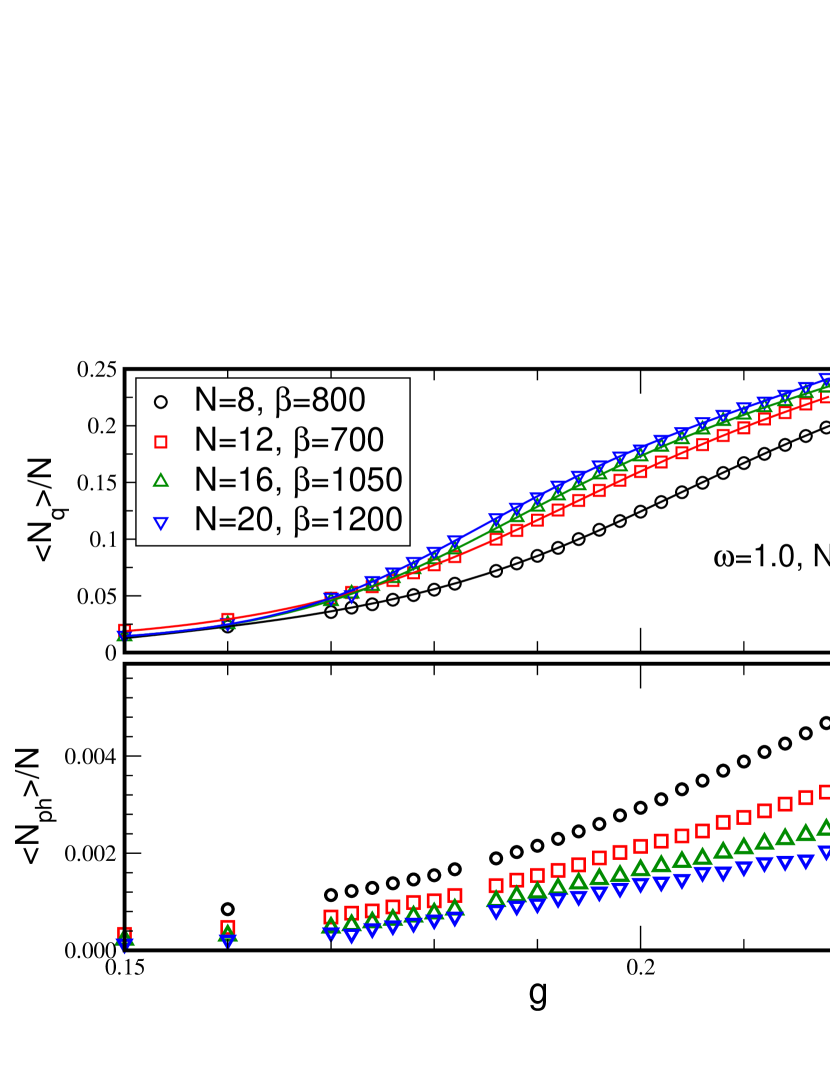
Figure 2: (Color online) Top: The order parameter, $\langle N_{q}\rangle/N$, versus $g$ for several system sizes. The $\beta$ values were chose such that the system is in the ground state. The solid curves going through the points are given by Padé approximants (see text). Bottom: The average photon density versus $g$.

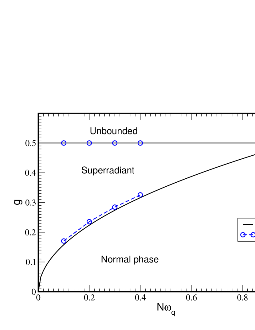
Figure 3: (Color online) Phase diagram of the Dicke model given by mean field and SGF QMC simulations. The QMC results are extrapolated to the thermodynamic limit.

In order to determine the transition point for each system size, we fit Padé approximants to the order parameter as a function of $g$ for each system size. The approximants we use are of the form,

$$P(x)=\frac{a+bx+cx^{2}+dx^{3}}{1+ex+fx^{2}+hx^{3}};$$ (17)

the maximum of the derivative yields the transition point for that system size. We then extrapolate the value of the critical $g$ to the thermodynamic limit. To determine the boundary between the superradiant phase and the unstable region, we calculate $\langle N_{ph}\rangle/N$ as a function of $g$ for a fixed $N\omega_{q}$. We find that as $g\to 1/2$, the photon density increases very rapidly and becomes unmanageable at $g=1/2$ indicating the instability. This way we map the phase diagram shown in Fig. 3 and which agrees very well with the MF solution. This excellent agreement can be understood as being due to the fact that the photon mode is coupled to all particles and introduces an effective long range interaction.

IV The Jaynes-Cummings-Hubbard Model

We now consider the JCH model given by Eq. (2) but ignoring the CR terms,

$$H_{JC} = -J\sum_{i=1}^{N}\left({\hat{a}}^{\dagger}_{i}{\hat{a}}^{\phantom{\dagger}}_{i+1}+h.c.\right)+\sum_{i=1}^{N}\left(\omega{\hat{a}}^{\dagger}_{i}{\hat{a}}^{\phantom{\dagger}}_{i}+\omega_{q}\sigma^{+}_{i}\sigma^{-}_{i}\right)$$ (18)

$$+g\sum_{i=1}^{N}\left(\sigma^{+}_{i}{\hat{a}}^{2}_{i}+\sigma^{-}_{i}{\hat{a}}^{\dagger 2}_{i}\right).$$

In what follows, we set the energy scale by fixing $g=1$.

IV.1 Perturbation

We start in the $J\ll 1$ limit where perturbation in $J$ can be expected to give accurate results.

In the $J=0$ limit, the model can be solved exactly since the eigenstates are dressed excitons labeled by the exciton number, $n$, and upper or lower branch, $\pm$, which can be written as a superposition of a Fock state with $n$ photons plus atomic ground state, $|n,g\rangle$, and a Fock state with $n-2$ photons plus atomic excited state, $|n-2,e\rangle$,

$$|n,+\rangle=\sin\theta_{n}|n,g\rangle+\cos\theta_{n}|n-2,e\rangle$$

$$|n,-\rangle=\cos\theta_{n}|n,g\rangle-\sin\theta_{n}|n-2,e\rangle$$ (19)

with the angle $\tan\theta_{n}=2g\sqrt{n(n-1)}/(\Delta+R_{n})$, $R_{n}(\Delta)=\sqrt{4g^{2}n(n-1)+\Delta^{2}}$, and the detuning parameter $\Delta=\omega_{q}-2\omega$.

The corresponding eigenvalues are

$$E_{n\pm}=n\omega+\Delta/2\pm R_{n}(\Delta)/2.$$ (20)

The zero-exciton state $|0-\rangle$ is a special case with $E_{0-}=0$. The energy difference $R_{n}(\Delta)$ defines the Rabi splitting of the upper and the lower branches. By comparing the energy of neighboring exciton number $n=2$ , we obtain the border $\omega\omega_{q}<1$ between vacuum and the $n=2$ Mott state. Leaving the $n=2$ Mott state or the vacuum at $\omega_{q}>1$ by increasing exciton number, renders the Hamiltonian unbounded from below and makes the system unstable at $\omega=1$. The $J=0$ phase diagram is shown in Fig. 4.

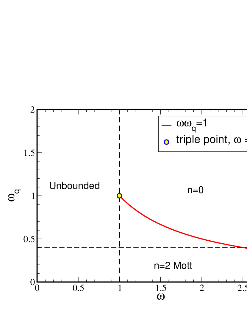
Figure 4: (Color online) Phase diagram of the two-photon JC Hubbard model in the $J=0$ limit. The horizontal dashed line at $\omega_{q}=0.4$ will be discussed below.

At small nonzero tunneling, $J\ll 1$, we ignore the upper exciton branch and perform a perturbation calculation to second order in $J$ to obtain the phase diagram of the JCH model. The ground state energy of the Mott phase, $E_{M}$, that of the state with one additional exciton, $E_{d}$, and that of the state with two additional excitons $E_{2d}$ are calculated. We find that the energy at the line determined by $E_{M}=E_{d}$ is smaller than $E_{2d}$ at the same $\omega$. This tells us that the upper Mott boundary is determined by doping with a single exciton (adding one photon). The boundary is given by,

$$\begin{split}&2\omega+(R_{2}-R_{3})-4Jt^{(3)2}_{--}+8J^{2}\Biggl{[}t_{--}^{(2)2}\\ &\left(-\sum_{\sigma=\pm}\frac{2t_{\sigma-}^{(3)2}}{\Delta-2R_{2}-\sigma R_{3}}+\frac{t_{--}^{(3)2}}{\Delta-2R_{2}+R_{3}}\right)\\ &+\sum_{\sigma=\pm}\frac{t_{\sigma-}^{(4)2}}{\Delta-R_{2}-R_{3}-\sigma R_{4}}\\ &+\frac{t_{+-}^{(3)2}t_{-+}^{(3)2}}{-2R_{2}-2R_{3}}-\frac{t_{+-}^{(3)2}t_{--}^{(3)2}}{R_{3}}-\frac{t_{--}^{(3)2}t_{-+}^{(3)2}}{-2R_{2}}\Biggr{]}=0,\end{split}$$ (21)

where the matrix elements

$$t^{(n)}_{\sigma\nu}=\mbox{$\langle n,\sigma|$}{\hat{a}}^{\dagger}\mbox{$|n-1,\nu\rangle$},$$ (22)

and $\sigma,\nu=\pm$, can be expressed in terms of the angle $\theta_{n}$ and exciton number $n$. See Appendix C for details.

To determine the lower Mott boundary, we remove one exciton (single holon doping) and calculate $E_{h}$, and also remove two excitons (double holon doping) and calculate $E_{2h}$. The energy $E_{h}$ is always higher than $E_{2h}$ at $\omega$ determined by $E_{M}=E_{2h}$ indicating that the lower boundary of the Mott phase is given by $E_{M}=E_{2h}$,

$$\begin{split}4\omega+\Delta-R_{2}+16J^{2}t_{--}^{(2)}\biggl{[}\frac{t_{--}^{(3)2}}{\Delta+R_{3}-2R_{2}}\\ +\frac{t_{+-}^{(3)2}}{\Delta-R_{3}-2R_{2}}-\frac{1}{\Delta-R_{2}}\biggr{]}=0.\end{split}$$ (23)

It is very interesting that, whereas single exciton doping determines the upper boundary, two excitons should be removed to determine the lower Mott boundary. This is confirmed by numerical calculations and has other consequences which will be discussed below. The natures of the phases above and below the Mott lobe will be discussed below.

The boundary between the vacuum and a state with at least two excitons is determined by the equation $E_{2e}=E_{0-}=0$, where $E_{2e}$ is the energy of the 2-exciton state:

$$4w+\Delta-R_{2}+\frac{16J^{2}t_{--}^{(2)2}}{\Delta-R_{2}}=0.$$ (24)

The resulting phase diagram, with the choice $\omega_{q}=0.4$, is shown in Fig. 5. Details of our perturbation calculation are shown in Appendix C. In addition, Fig. 5 shows the mean field boundary (see Appendix B for details), Eq. (56), between stable thermodynamic phases and the unstable region where the Hamiltonian is unbounded from below. For comparison, we also show in Fig. 5 the phase boundaries obtained with DMRG. As expected, we see very good agreement between perturbation and DMRG for small values $J$.

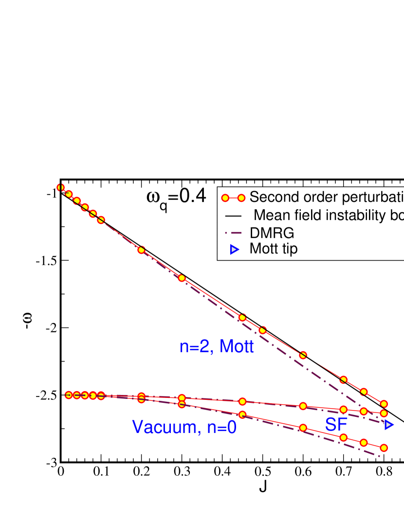
Figure 5: (Color online) The phase diagram of the two-photon JCH model. The phase boundaries from second order perturbation are given by the circles. The mean field instability boundary is shown by the solid line. For comparison, we include the phase boundaries from DMRG calculations (see below). We do not show all the numerical results here to keep the figure uncluttered (see Fig. 9).

IV.2 Numerical results

To obtain the phase diagram with exact numerical methods, we employ the SGFrousseau08 ; rousseau08b quantum Monte Carlo method and DMRGwhite92 ; white93 using the ALPSalps library. The SGF and DMRG methods offer complementary advantages and allow us to map out the phase diagram more precisely. Some typical running times for the SGF QMC simulations are: $216$ hours for $N=24$ at $\beta=768$ and $192$ hours for $N=20$ at $\beta=640$. These long running times and large values of $\beta$ are necessary to ensure convergence to the ground state. As for DMRG, we typically took the maximum number of photons/site, $N_{max}=5$, $500$ states, and $500$ sweeps. These values are typical but the details depend on the couplings and the phase of the system. In all cases, we verified that increasing these values did not change the results.

As in the previous section, here we set the energy scale by fixing $g=1$ and take $\omega_{q}=0.4$. We start with grand canonical QMC simulations using the SGF algorithm. Figure 6 shows the density of excitons as a function of the photon frequency, $\omega$, for several values of the inverse temperature $\beta$. This allows us to determine how large $\beta$ needs to be to probe the ground state. Note that in the grand canonical ensemble, $\omega$ is minus the photon chemical potential. We see a clear incompressible Mott insulator (MI) plateau surrounded by compressible regions. We note that the MI becomes fully formed only for very large $\beta$. This is due to the small value of $J$ we chose for the figure; larger values of $J$ do not require such high values of $\beta$, but, of course, at larger $J$, the MI is not as wide (see Fig. 5).

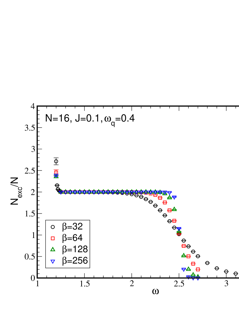
Figure 6: (Color online) The dependence of the exciton density on the photon frequency, $\omega$. The horizontal line indicates the existence of an incompressible Mott insulating phase surrounded by two compressible phases.

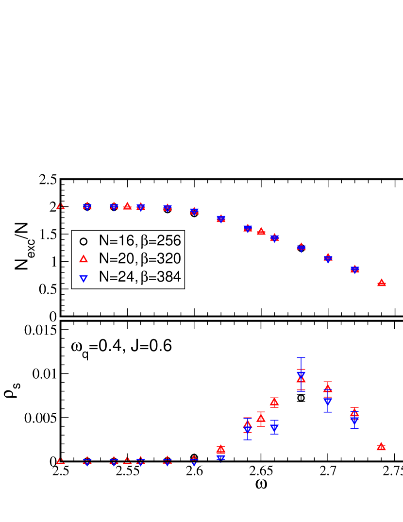
Figure 7: (Color online) Top: The exciton density as a function of $\omega$. Bottom: The corresponding superfluid density, $\rho_{s}$, as a function of $\omega$. This shows that as the MI is doped with holes, a superfluid phase appears.

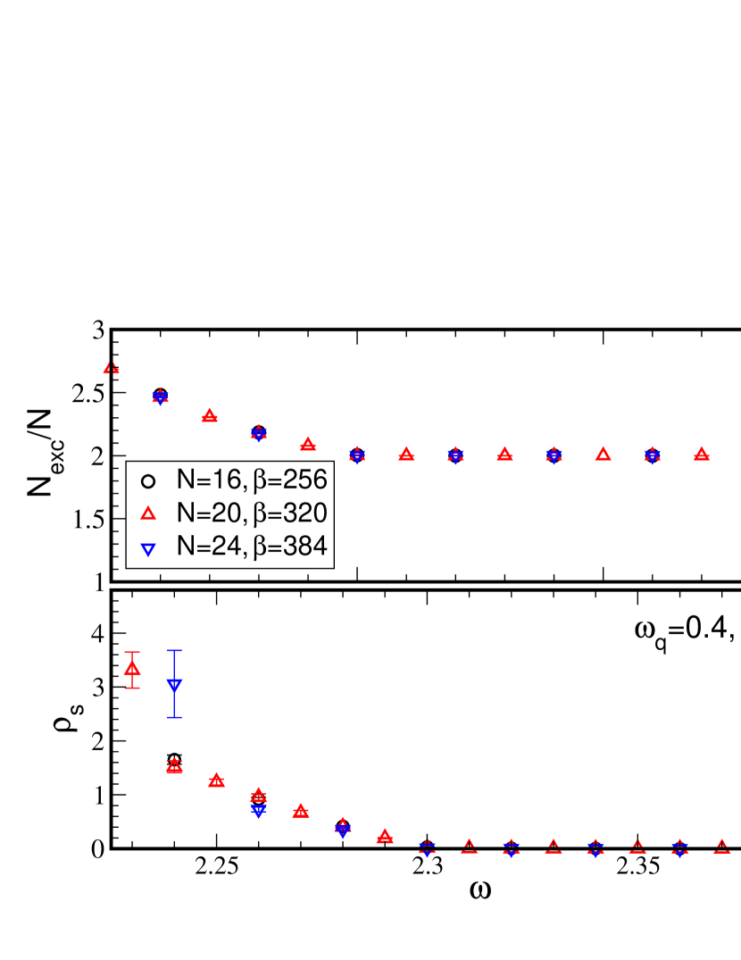
Figure 8: (Color online) Same as Fig. 7 but doping the MI with particles. A superfluid phase appears here too.

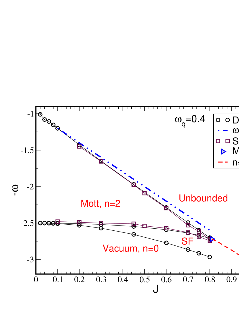
Figure 9: (Color online) The phase diagram of the JCH model from SGF QMC and DMRG calculations. Dash-double dot line ($\omega=2J+g$) is the MF boundary between the unstable and stable regions. The (blue) right triangle indicates the position of the tip of the Mott lobe. The dashed (red) line indicates the SF phase with a density of $2$ excitons/site. This is the same as Fig. 5 but not showing the perturbation results for clarity.

To delineate the nature of the compressible regions surrounding the MI, we show in Figs. 7 and 8 the exciton density as a function of $\omega$ in the top panel, and the superfluid density, $\rho_{s}$, in the bottom panel. We see in both figures that, as soon as the system leaves the MI phase, it becomes superfluid. Hole doping, Fig. 7, results in a very dilute SF before the system eventually becomes empty as $\omega\approx 2.8$. Particle doping, Fig. 8, leads to a SF with $\rho_{s}$ approaching $2$ before the system starts to become unstable at $\omega\approx 2.23$. By making several cuts of this type, we map out the phase diagram shown in Fig. 9 obtained numerically with very good agreement between SGF and DMRG. The figure shows a single Mott lobe with $2$ excitons/site; below this lobe there is a rather narrow region of SF before the system becomes empty. Above the Mott lobe, there is an even narrower strip of SF before the system becomes unstable. It is hard to pinpoint precisely with SGF and DMRG the boundary where the system becomes unstable because the number of photons/site increases very rapidly near the instability. Neither DMRG nor QMC performs well under such conditions and, for that reason, we show in the figure the stable/unstable boundary given by MF calculations. Unlike the case of the 1-photon JCMrossini07 , there are no higher Mott lobes in this 2-photon case due to the instability triggered by the Hamiltonian becoming unbounded from below. The Mott lobe terminates in a cusp because the critical point at the tip is in the BKT universality class.

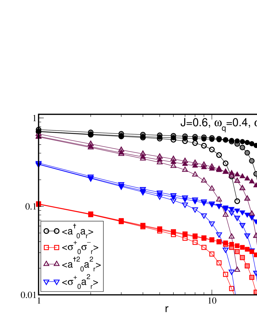
Figure 10: (Color online) Photon-photon, photon-qubit and qubit-qubit Green functions from DMRG in the SF region above the MI. The open, shaded and full symbols are for $N=30,40$ and $50$ respectively.

Figure 11: (Color online) Same as Fig. 10 but below the Mott lobe. The open, shaded symbols are for $N=30,50$ respectively.

The question arises as to the nature of the SF phase. In the 1-photon systemrossini07 , the photon Green function, $\langle{\hat{a}}^{\dagger}_{0}{\hat{a}}^{\phantom{\dagger}}_{r}\rangle$ decays as a power indicating quasi-long range order and a photon SF. At the same time, the photon-qubit Green function, $\langle\sigma^{+}_{0}{\hat{a}}^{\phantom{\dagger}}_{r}\rangle$, also decays as a power law. We see the same behavior in Fig. 10 where several two-point functions are shown on log-log scale. We note, in particular, that $\langle{\hat{a}}^{\dagger}_{0}{\hat{a}}^{\phantom{\dagger}}_{r}\rangle$ decays as a power law, and that, while both $\langle{\hat{a}}_{0}^{\dagger 2}{\hat{a}}_{r}^{2}\rangle$ and $\langle\sigma^{+}_{0}{\hat{a}}^{2}_{r}\rangle$ decay as powers, they are not equal. The leading effect in this phase is then the coherent movement of individual photons.

One expects to encounter similar behavior below the Mott lobe. However, this expectation is not borne out by the numerical results. Figure 11 shows the same correlation functions as Fig. 10 where we see clearly that, although the system is in the SF phase, the quantity $\langle{\hat{a}}_{0}^{\dagger}{\hat{a}}_{r}\rangle$ decays exponentially while it exhibited power law behavior above the MI. The correlation functions $\langle\sigma^{+}_{0}\sigma^{-}_{r}\rangle$ and $\langle{\hat{a}}^{\dagger 2}_{0}{\hat{a}}^{2}_{r}\rangle$ both decay as powers showing the SF nature of this phase. In addition, we find that, unlike the case above the MI (see Fig. 10), the correlation function $\langle\sigma^{+}_{0}{\hat{a}}^{2}_{r}\rangle$ is identical to $\langle{\hat{a}}^{\dagger 2}_{0}{\hat{a}}^{2}_{r}\rangle$, and so we do not show it in Fig.11 to keep the figure clear.

This behavior appears to show that above the MI, we have a photon SF phase (power law decay for $\langle{\hat{a}}^{\dagger}_{0}{\hat{a}}^{\phantom{\dagger}}_{r}\rangle$) whereas below the MI we have a photon pair SF phase (exponential decay of $\langle{\hat{a}}^{\dagger}_{0}{\hat{a}}^{\phantom{\dagger}}_{r}\rangle$ and power law decay of $\langle{\hat{a}}^{\dagger 2}_{0}{\hat{a}}^{2}_{r}\rangle$): Below the Mott insulator the photons appear to form bound pairs which become superfluid.

V The Rabi-Hubbard model

Figure 12: (Color online) The mean field phase diagram of the RH model exhibiting normal and superradiant phases and an unbounded region. This behavior is similar to that of the Dicke model.

In Appendix A we show the mean field calculation for the Rabi-Hubbard model predicting a phase transition between a disordered (normal) phase and a superradiant phase similar to the Dicke modelgarbe17 . The boundary between the two phases is given by (see Eq. (48))

$$E_{G}({\bar{b}}\neq 0,g,J,\omega,\omega_{q})=E_{G}({\bar{b}}=0,g,J,\omega,\omega_{q}),$$ (25)

where $E_{G}$ is the ground state energy given by (see Eq. (48)

$$E_{G} = \frac{1}{2}\sum_{k}\biggl{[}\sqrt{(-2J\cos(k)+\omega)^{2}-16g^{2}{\bar{b}}^{2}+16g^{2}{\bar{b}}^{4}}$$

$$+ \omega_{q}{\bar{b}}^{2}-\frac{\omega}{2}\biggr{]}.$$

In addition, the stability condition requires (see Eq. (49),

$$\omega-2J\geq 2g.$$ (27)

The two phases and the unstable region are shown in Fig. 12. This phase diagram is the analog of that of the Dicke model, Fig. 3. However, whereas in the case of the Dicke model, we found excellent agreement between the MF and QMC phase diagrams (Fig. 12), this is not the case for the RH model.

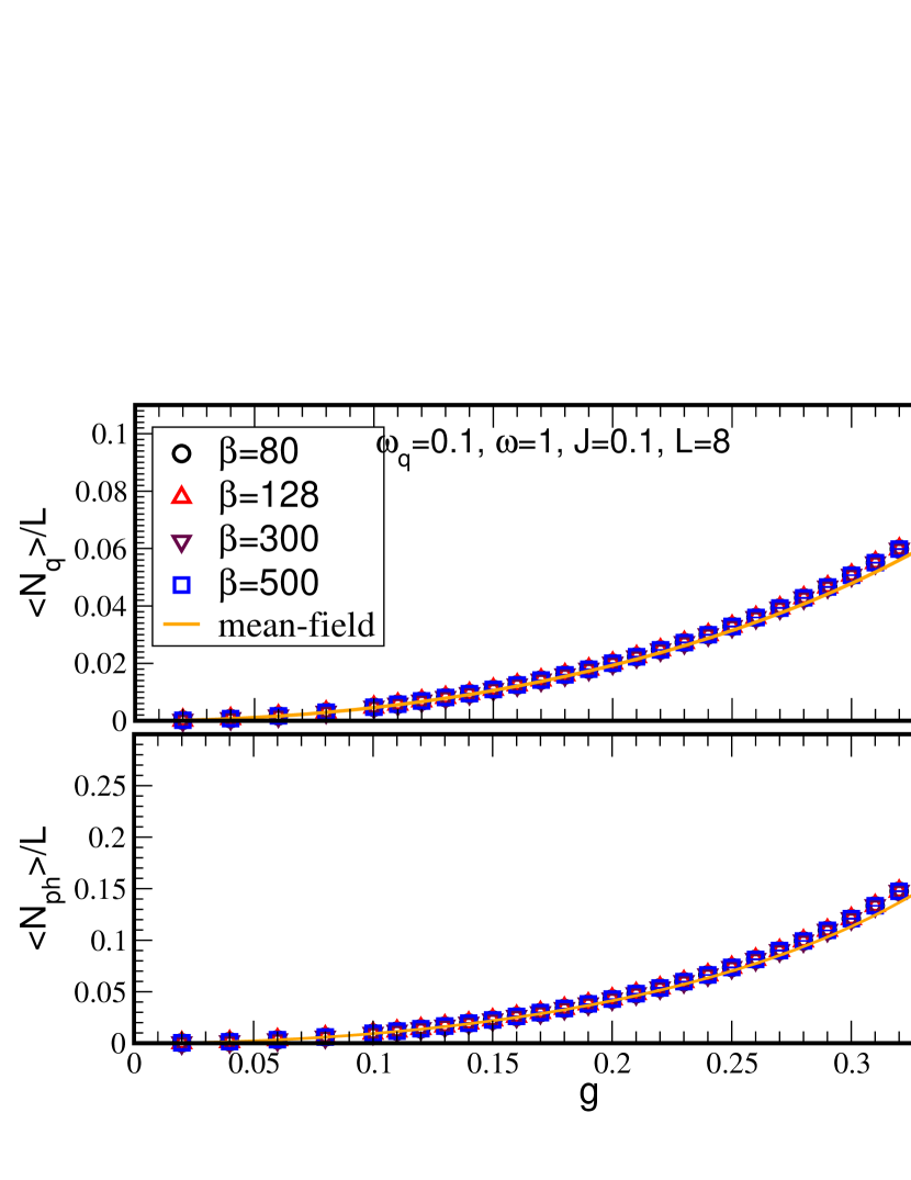
Figure 13: (Color online) Excited qubit density, $\langle N_{q}\rangle/N$, (upper panel) and photon density (lower panel) as functions of $g$. Various $\beta$ values are used to make sure the system is in the ground state.

We show in Fig. 13 the average number of excited qubits, $\langle N_{q}\rangle/N$, (top) and the average photon density, $\langle N_{ph}\rangle/N$, (bottom) as functions of the coupling $g$ for several values of $\beta$. We observe a smooth continuous increase of both quantities as $g$ increases and no finite temperature effects. The values are in good agreement with the mean-field approach described in Appendix B, which, for the parameters of Fig. 13, predicts a direct transition from a normal phase to the unbounded region. On the other hand, since the same mean-field approach applied to the JCH Hamiltonian is not able to capture the photon pair SF phase, it is possible that it also misses an SF phase in the RH model for parameters different from shown in the figure. In Fig. 14, we show that for sufficiently large $\beta$ there is no finite size effects. Comparing the top panels of Figs. 13 and 14 with Fig. 1 emphasizes the difference in behavior between the two models and suggests the absence of a phase transition for the RH model, at least for the present parameter values. For the entire range of values of $g$ in Figs.13 and 14, all Green functions, such as $\langle{\hat{a}}^{\dagger}_{0}{\hat{a}}_{r}\rangle$ and $\langle\sigma^{+}_{0}{\hat{a}}^{2}_{r}\rangle$, decay exponentially indicating a normal rather than a superradiant phase.

In short, at least for the parameter values we have considered, the Rabi-Hubbard model seems not to exhibit a phase transition, even though the underlying discrete $Z_{4}$ symmetry allows it. In addition, we have two different mean-field approaches leading to rather different phase diagrams, which seems to indicate that the physics of the Rabi-Hubbard model might be more involved than the one of the Dicke and the JC models. A thorough study is beyond the scope of the present paper and will be presented elsewhere.

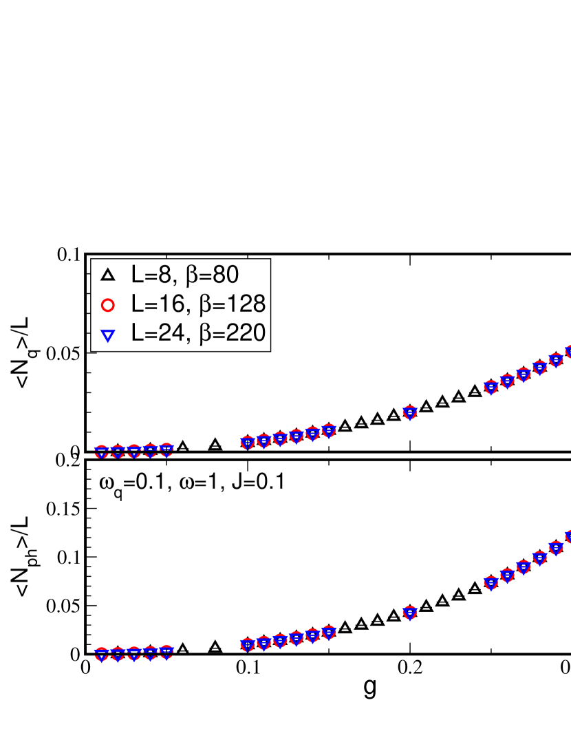
Figure 14: (Color online) The same as fig. 13 but for different system sizes showing that finite size effects are negligible.

VI Conclusions

In this paper we studied the ground state properties of the Dicke, Jaynes-Cummings Hubbard, and Rabi-Hubbard models. We used mean field, perturbation, QMC, and DMRG calculations to elucidate the phase diagrams and the transitions between the various phases. We found that for the Dicke model, exact QMC results agree very well with the mean field phase diagramgarbe17 but that very large $\beta$ was required to probe the ground state properties. For the JCH model, we found that at small hopping, $J$, the system exhibits a single incompressible Mott insulator with two excitons/site. Doping above the MI, the system exhibits a photon SF phase before becoming unstable due to the Hamiltonian becoming unbounded from below. To dope the system above the MI, we add one photon at a time. This is in big contrast to the situation below the MI where we found a surprising photon pair SF: The photons pair up in bound states. Below the MI, one needs to remove two photons at a time to dope. For the JCH model in the SF phase, very large values of $\beta$ are needed. Interestingly, we have not found a phase transition between a normal and a superradiant phase in the case of the RH model; only a normal phase with exponential decay of the Green functions. It would be interesting to study how the three-photon model would differ from what we found here. In particular,would the JCH model still exhibit a MI phase, and would doping below it yield a three-photon bound state superfluid.

Appendix A Mean field two-photon RH

In this appendix we outline the mean field calculation of the phase diagram of the two-photon Rabi-Hubbard model which proceeds along the same lines as that for the Dicke model in garbe17, . The RH Hamiltonian is:

$$H_{RH} = -J\sum_{i}\left({\hat{a}}^{\dagger}_{i}{\hat{a}}^{\phantom{\dagger}}_{i+1}+h.c.\right)+\sum_{i}\left(\omega_{q}\sigma^{+}_{i}\sigma^{-}_{i}+\omega{\hat{a}}^{\dagger}_{i}{\hat{a}}^{\phantom{\dagger}}_{i}\right)$$ (28)

$$+g\sum_{i}\left(\sigma^{+}_{i}+\sigma^{-}_{i}\right)\left({\hat{a}}^{\dagger\,2}_{i}+{\hat{a}}^{2}_{i}\right).$$

We apply the Holstein-Primakoff transformation:

$$\sigma^{+}_{i} = {\hat{b}}^{\dagger}_{i}\sqrt{1-{\hat{b}}^{\dagger}_{i}{\hat{b}}^{\phantom{\dagger}}_{i}}$$ (29)

$$\sigma^{-}_{i} = \sqrt{1-{\hat{b}}^{\dagger}_{i}{\hat{b}}^{\phantom{\dagger}}_{i}}\,{\hat{b}}^{\phantom{\dagger}}_{i},$$ (30)

with $[{\hat{b}}^{\phantom{\dagger}}_{i},{\hat{b}}^{\dagger}_{j}]=\delta_{ij}$, use the mean field approximation,

$${\bar{b}}^{*} = \langle GS|{\hat{b}}^{\dagger}_{i}|GS\rangle,$$ (31)

$${\bar{b}} = \langle GS|{\hat{b}}^{\phantom{\dagger}}_{i}|GS\rangle,$$ (32)

$${\bar{b}} = {\bar{b}}^{*},$$ (33)

and ignore fluctuations in the ${\hat{b}}$ field. This leads to the quadratic mean field Hamiltonian,

$$H_{MF} = -J\sum_{i}\left({\hat{a}}^{\dagger}_{i}{\hat{a}}^{\phantom{\dagger}}_{i+1}+{\hat{a}}^{\dagger}_{i+1}{\hat{a}}^{\phantom{\dagger}}_{i}\right)+\omega\sum_{i}{\hat{a}}^{\dagger}_{i}{\hat{a}}^{\phantom{\dagger}}_{i}$$ (34)

$$+2g{\bar{b}}\sqrt{1-{\bar{b}}^{2}}\sum_{i}\left({\hat{a}}^{\dagger\,2}_{i}+{\hat{a}}^{2}_{i}\right)$$

$$+N_{s}\omega_{q}{\bar{b}}^{2}.$$

Applying a Fourier transform,

$${\hat{a}}_{i}=\frac{1}{\sqrt{N}}\sum_{i}{\rm e}^{-ikr_{i}}{\hat{a}}_{k},$$ (35)

leads to,

$$H_{MF} = \sum_{k}\bigg{[}\left(-2J\cos(k)+\omega\right){\hat{a}}^{\dagger}_{k}{\hat{a}}^{\phantom{\dagger}}_{k}$$ (36)

$$+2g{\bar{b}}\sqrt{1-{\bar{b}}^{2}}\left({\hat{a}}^{\dagger}_{k}{\hat{a}}^{\dagger}_{-k}+{\hat{a}}^{\phantom{\dagger}}_{k}{\hat{a}}^{\phantom{\dagger}}_{-k}\right)\bigg{]}$$

$$+N_{s}\omega_{q}{\bar{b}}^{2}.$$

Now, we use the Bogoliubov transformation:

$${\hat{a}}^{\dagger}_{k} = {\rm cosh}(X_{k}){\hat{\alpha}}^{\dagger}_{k}-{\rm sinh}(X_{k}){\hat{\alpha}}^{\phantom{\dagger}}_{-k}$$ (37)

$${\hat{a}}^{\phantom{\dagger}}_{k} = {\rm cosh}(X_{k}){\hat{\alpha}}^{\phantom{\dagger}}_{k}-{\rm sinh}(X_{k}){\hat{\alpha}}^{\dagger}_{-k}.$$ (38)

To simplify the expressions, we write: $c_{k}\equiv{\rm cos}(k)$, $ch_{k}\equiv{\rm cosh}(X_{k})$, and $sh_{k}\equiv{\rm sinh}(X_{k})$. This yields,

$$H_{MF} = \sum_{k}\bigg{[}\left(-2Jc_{k}+\omega\right)\left(ch_{k}^{2}+sh_{k}^{2}\right)$$ (39)

$$-8g{\bar{b}}\sqrt{1-{\bar{b}}^{2}}\,ch_{k}sh_{k}\bigg{]}{\hat{\alpha}}^{\dagger}_{k}{\hat{\alpha}}^{\phantom{\dagger}}_{k}$$

$$+ \sum_{k}\bigg{[}\bigg{(}2g{\bar{b}}\sqrt{1-{\bar{b}}^{2}}\,(ch_{k}^{2}+sh_{k}^{2})$$

$$-(-2Jc_{k}+\omega)ch_{k}sh_{k}\bigg{)}{\hat{\alpha}}^{\dagger}_{k}{\hat{\alpha}}^{\dagger}_{-k}+{\rm h.c.}\bigg{]}$$

$$+ \sum_{k}\bigg{[}(-2Jc_{k}+\omega)sh_{k}^{2}$$

$$-4g{\bar{b}}\sqrt{1-{\bar{b}}^{2}}\,ch_{k}sh_{k}\bigg{]}+N_{s}\omega_{q}{\bar{b}}^{2}.$$

The first term in Eq. (39) gives the quasi-particle excitations above the ground state; the second term contains the nondiagonal terms which we want to eliminate and the third term gives the ground state energy. When the coefficient of the nondiagonal term is made to vanish, we obtain the condition:

$$2g{\bar{b}}\sqrt{1-{\bar{b}}^{2}}\,(ch_{k}^{2}+sh_{k}^{2})=(-2Jc_{k}+\omega)ch_{k}sh_{k},$$ (40)

and using

$${\rm sinh}(2x) = 2{\rm sinh}(x){\rm cosh}(x),$$

$${\rm cosh}(2x) = {\rm sinh}^{2}(x)+{\rm cosh}^{2}(x),$$ (41)

we get:

$${\rm tanh}(2X_{k})=\frac{4g{\bar{b}}\sqrt{1-{\bar{b}}^{2}}}{\omega-2J{\rm cos}(k)}.$$ (42)

Writing

$$A=2g{\bar{b}}\sqrt{1-{\bar{b}}^{2}},\,\,\,\,\,\,B_{k}=\omega-2J{\rm cos}(k),$$ (43)

gives:

$${\rm tanh}(2X_{k})=\frac{2A}{B_{k}},$$ (44)

and,

$${\rm e}^{X_{k}}=\left[\frac{B_{k}+2A}{B_{k}-2A}\right]^{1/4}.$$ (45)

The acceptable values satisfy the condition:

$$-1\leq\frac{2A}{B_{k}}\leq 1.$$ (46)

Then, the energy that must be minimized with respect to ${\bar{b}}$ is

$$E_{G} = \sum_{k}\bigg{[}(-2Jc_{k}+\omega)sh_{k}^{2}-4g{\bar{b}}\sqrt{1-{\bar{b}}^{2}}\,ch_{k}sh_{k}\bigg{]}$$ (47)

$$+N_{s}\omega_{q}{\bar{b}}^{2}.$$

Note that, putting $J=0$, renders all the hyperbolic functions independent of $k$. Then Eq. (47) agrees with the MF equation in Ref. garbe17, if we take $N=1$ and ${\bar{b}}={\bar{b}}^{*}$.

Equation (47) can be further simplified to the form,

$$E_{G} = \frac{1}{2}\sum_{k}\biggl{[}\sqrt{(-2J\cos(k)+\omega)^{2}-16g^{2}{\bar{b}}^{2}+16g^{2}{\bar{b}}^{4}}$$ (48)

$$+ \omega_{q}{\bar{b}}^{2}-\frac{\omega}{2}\biggr{]}.$$

The requirement that the argument of the square root be positive leads to the important condition:

$$\omega-2J\geq 2g.$$ (49)

This is the stability condition for the system: When it is violated, the Hamiltonian is unbounded from below.

The transition to the superradiant phase is indicated by a nonzero order parameter of the order parameter, ${\bar{b}}\neq 0$. The boundary between the normal and superradiant phases is, therefore, given by:

$$E_{G}({\bar{b}}\neq 0,g,J,\omega,\omega_{q})=E_{G}({\bar{b}}=0,g,J,\omega,\omega_{q}).\quad$$ (50)

This relation cannot be solved analytically, we solve it numerically to get the relation between $g,J,\omega,\omega_{q}$ which gives the phase boundary.

Appendix B Simple mean field for JCH

The mean field calculation in Appendix A applies to the Rabi-Hubbard model and, by ignoring the counter-rotating terms, also to the JCH model. However, we can also perform the mean field calculation on the hopping term of the photon field rather than on the qubit. We assume $\langle a_{i}\rangle=\psi_{i}$, which reduces the Hamiltonian to a single-site form:

$$H_{i}^{MF}= -J\left((\psi_{i+1}+\psi_{i-1})a^{\dagger}_{i}+\text{h.c.}\right)$$ (51)

$$+\omega_{q}\sigma_{i}^{+}\sigma_{i}^{-}+\omega a^{\dagger}_{i}a_{i}+g\left(\sigma^{+}_{i}+\sigma^{-}_{i}\right)\left({\hat{a}}^{\dagger\,2}_{i}+{\hat{a}}^{2}_{i}\right).$$

Finding the ground state of this Hamiltonian and a self-consistent solution for the $\psi_{i}$ allows us to obtain the phase diagram. In particular, in the normal phase $\psi_{i}=0$, the ground state of $H_{i}^{MF}$ still depends on the parameters $\omega_{q}$, $\omega$ and $g$, leading, for instance, to the dependence of the qubit and photon densities on the interaction strength observed in Fig.13.

A further approximation amounts to replacing all the photonic operators by the mean field value, $\psi$, thus yielding the leading order contribution which gives the instability line for the JCH model. In that case, assuming that $\psi$ is real, the mean field Hamiltonian becomes

$$H_{i}^{SMF} = \omega_{q}\sigma_{i}^{+}\sigma_{i}^{-}+\omega\psi^{2}+g(\sigma_{i}^{+}+\sigma_{i}^{-})\psi^{2}-2J\psi^{2}.$$

The ground state energy is found by minimizing

$$E_{G}=\frac{\omega_{q}}{2}+(\omega-2J)\psi^{2}-\frac{\sqrt{\omega_{q}^{2}+4g^{2}\psi^{4}}}{2},$$ (53)

with respect to $\psi$ which gives

$$\omega-2J=\frac{2g^{2}\psi^{2}}{\sqrt{\omega_{q}^{2}+4g^{2}\psi^{4}}}.$$ (54)

Near the unbounded region, $\psi\gg 1$ and we can thus ignore the $\omega_{q}$ term and find that for stability we must have,

$$\omega-2J\geq g.$$ (55)

The boundary of the unstable region is therefore given by,

$$\omega_{c}-2J=g.$$ (56)

Note the similarity between this equation and the stability condition for the RHM, Eq. (49).

We then define the photon density $n_{ph}=\psi^{2}$ and, using Eq. (54) we obtain,

$$n_{ph}=\frac{\omega_{q}(\omega-2J)}{2g}\frac{1}{\sqrt{(g-\omega+2J)(g+\omega-2J)}}.\quad$$ (57)

Now we consider $\omega$ near the stable-unstable boundary, $\omega_{c}$, so that $\omega-2J\approx g$. We find that the number of photons diverges as the unstable region is approached:

$$n_{ph}=\frac{\omega_{q}}{2\sqrt{2g}}\frac{1}{\sqrt{2J+g-\omega}}\propto(\delta\omega)^{1/2},$$ (58)

with $\delta\omega=\omega_{c}-\omega$. This divergence makes the result difficult to demonstrate with QMC and/or DMRG methods.

Appendix C Perturbation calculation of the phase diagram of the JCH model

In this appendix we outline the perturbation calculation of the phase diagram of the two-photon JCH model which proceeds along the same lines as that for the single-photon JCH model in schmidt09, .

The Hamiltonian of the two-photon JCH model is

$$H_{JC} = -J\sum_{i=1}^{N}\left({\hat{a}}^{\dagger}_{i}{\hat{a}}^{\phantom{\dagger}}_{i+1}+h.c.\right)+\sum_{i=1}^{N}\left(\omega{\hat{a}}^{\dagger}_{i}{\hat{a}}^{\phantom{\dagger}}_{i}+\omega_{q}\sigma^{+}_{i}\sigma^{-}_{i}\right)$$ (59)

$$+g\sum_{i=1}^{N}\left(\sigma^{+}_{i}{\hat{a}}^{2}_{i}+\sigma^{-}_{i}{\hat{a}}^{\dagger 2}_{i}\right).$$

which can be split into two parts,

$$H_{JC}=H_{0}+H_{1},$$ (60)

with the perturbation, $H_{1}$, given by

$$H_{1}=-J\sum_{i}(a^{\dagger}_{i}a_{i+1}+h.c.),$$ (61)

and $H_{0}$ is the rest of $H$.

It is convenient to introduce the matrix elements

$$t^{(n)}_{\sigma\nu}\equiv\mbox{$\langle n,\sigma|$}a^{\dagger}\mbox{$|n-1,\nu\rangle$},$$ (62)

with $\sigma,\nu=\pm$. Using Eq. (19), we have

$$a^{\dagger}\mbox{$|n-1,+\rangle$} = t^{(n)}_{++}\mbox{$|n,+\rangle$}+t^{(n)}_{-+}\mbox{$|n,-\rangle$},$$

$$a^{\dagger}\mbox{$|n-1,-\rangle$} = t^{(n)}_{+-}\mbox{$|n,+\rangle$}+t^{(n)}_{--}\mbox{$|n,-\rangle$},$$ (63)

with

$$t^{(n)}_{\sigma\nu}=\sqrt{n}\alpha^{\sigma}_{n}\alpha^{\nu}_{n-1}+\sigma\nu\sqrt{n-2}\alpha_{n}^{-\sigma}\alpha_{n-1}^{-\nu},$$ (64)

where

$$\alpha_{n}^{+}=\sin\theta_{n},$$

$$\alpha_{n}^{-}=\cos\theta_{n}.$$ (65)

For the upper boundary of the $n=2$ Mott phase, we compare the ground state energy of the $n=2$ Mott state with that of the state doped by one exciton. However, to determine the lower boundary of the $n=2$ Mott phase, we need to compare the ground state energy with the state doped by 2 holons (with two excitons removed from the system). Similarly, to locate the boundary of vacuum, we need to compare the energy of the state doped by two excitons with vacuum.

We first calculate the energy of the Mott state to second order,

$$E_{M}=E_{M}^{(0)}+E_{M}^{(1)}+E_{M}^{(2)},$$ (66)

with

$$E_{M}^{(0)} = \mbox{$\langle\psi_{M}^{(0)}|$}H_{0}\mbox{$|\psi_{M}^{(0)}\rangle$}=N(2\omega+\frac{\Delta}{2}-\frac{R_{2}}{2}),$$

$$E_{M}^{(1)} = \mbox{$\langle\psi_{M}^{(0)}|$}H_{1}\mbox{$|\psi_{M}^{(0)}\rangle$}=0,$$ (67)

$$E_{M}^{(2)} = \mbox{$\langle\psi_{M}^{(1)}|$}H_{1}\mbox{$|\psi_{M}^{(0)}\rangle$}=4J^{2}N\sum_{\sigma=\pm}\frac{t_{\sigma-}^{(3)2}t_{--}^{(2)2}}{\Delta-\sigma R_{3}-2R_{2}},$$

where the zero-th order wavefunction is

$$\mbox{$|\psi_{M}^{(0)}\rangle$}=\prod^{N}_{i}\mbox{$|2,-\rangle$}_{i},$$ (68)

and the first order wavefunction is

$$\mbox{$|\psi_{M}^{(1)}\rangle$}=\sum_{k}\frac{\mbox{$|k\rangle$}\mbox{$\langle k|$}H_{1}\mbox{$|\psi_{M}^{(0)}\rangle$}}{E_{M}^{(0)}-E_{k}}$$

$$=-J\sum_{i}\sum_{\sigma=\pm}\Biggl{[}\frac{t_{\sigma-}^{(3)}t_{--}^{(2)}\mbox{$|1,-\rangle$}_{i}\mbox{$|3,\sigma\rangle$}_{i+1}\prod^{N}_{l\neq i,l\neq i+1}\mbox{$|2,-\rangle$}_{l}}{\Delta-\sigma R_{3}-2R_{2}}$$

$$+\frac{t_{\sigma-}^{(3)}t_{--}^{(2)}\mbox{$|1,-\rangle$}_{i+1}\mbox{$|3,\sigma\rangle$}_{i}\prod^{N}_{l\neq i,l\neq i+1}\mbox{$|2,-\rangle$}_{l}}{\Delta-\sigma R_{3}-2R_{2}}\Biggr{]}.$$ (69)

Now we calculate the lowest energy of the state obtained by doping the $n=2$ Mott state, to second order,

$$E_{d}=E_{d}^{(0)}+E_{d}^{(1)}+E_{d}^{(2)},$$ (70)

with

$$E_{d}^{(0)} = \mbox{$\langle\psi_{d}^{(0)}|$}H_{0}\mbox{$|\psi_{d}^{(0)}\rangle$}$$

$$= (N-1)(2\omega+\frac{\Delta}{2}-\frac{1}{2}R_{2})+(3\omega+\frac{\Delta}{2}-\frac{R_{3}}{2}),$$

$$E_{d}^{(1)} = \mbox{$\langle\psi_{d}^{(0)}|$}H_{1}\mbox{$|\psi_{d}^{(0)}\rangle$}=-2Jt_{--}^{(3)2},$$

$$E_{d}^{(2)} = \mbox{$\langle\psi_{d}^{(1)}|$}H_{1}\mbox{$|\psi_{d}^{(0)}\rangle$}$$ (71)

$$= 4J^{2}\Biggl{[}\frac{t_{--}^{(3)2}t_{--}^{(2)2}}{\Delta+R_{3}-2R_{2}}+\sum_{\sigma=\pm}(\frac{(N-2)t_{\sigma-}^{(3)2}t_{--}^{(2)2}}{\Delta-2R_{2}-\sigma R_{3}}$$

$$+ \frac{t_{\sigma-}^{(4)2}t_{--}^{(2)2}}{\Delta-R_{2}-R_{3}-\sigma R_{4}}+\frac{t_{+-}^{(3)2}t_{-\sigma}^{(3)2}}{R_{3}-R_{2}-\sigma R_{2}}$$

$$+ \frac{t_{\sigma(-\sigma)}^{(3)2}t_{--}^{(3)2}}{-R_{3}-\sigma R_{3}-R_{2}+\sigma R_{2}})\Biggr{]},$$

where

$$\mbox{$|\psi_{d}^{(0)}\rangle$}=\frac{1}{\sqrt{N}}\sum_{i}\mbox{$|3,-\rangle$}_{i}\prod^{N}_{l\neq i}\mbox{$|2,-\rangle$}_{l},$$ (72)

and

$$\mbox{$|\psi_{d}^{(1)}\rangle$}=\mbox{$|\psi_{d}^{(1)}(1)\rangle$}+\mbox{$|\psi_{d}^{(1)}(2)\rangle$}+\mbox{$|\psi_{d}^{(1)}(3)\rangle$},$$ (73)

with

$$|\psi_{d}^{(1)}(1)\rangle = \frac{1}{\sqrt{N}}\sum_{i,j,\sigma=\pm}\frac{-2J}{\Delta-(\sigma)R_{3}-2R_{2}}t_{\sigma-}^{(3)}t_{--}^{(2)}$$

$$\times (\mbox{$|3,\sigma\rangle$}_{i}\mbox{$|1,-\rangle$}_{i+1}+\mbox{$|1,-\rangle$}_{i}\mbox{$|3,\sigma\rangle$}_{i+1})\mbox{$|3,-\rangle$}_{j\neq i,j\neq i+1}$$

$$\times \prod_{l\neq i,l\neq i+1,l\neq j}\mbox{$|2,-\rangle$}_{l},$$

$$|\psi_{d}^{(1)}(2)\rangle = \frac{1}{\sqrt{N}}\sum_{i,{\sigma=\pm}}\frac{-2J}{\Delta-R_{2}-R_{3}-(\sigma)R_{4}}t_{\sigma-}^{(4)}t_{--}^{(2)}$$

$$\times (\mbox{$|4,\sigma\rangle$}_{i}\mbox{$|1,-\rangle$}_{i+1}+\mbox{$|1,-\rangle$}_{i}\mbox{$|4,\sigma\rangle$}_{i+1})$$

$$\times \prod^{N}_{l\neq i,l\neq i+1}\mbox{$|2,-\rangle$}_{l},$$

$$|\psi_{d}^{(1)}(3)\rangle = \frac{1}{\sqrt{N}}\sum_{i}\biggl{[}\,\sum_{\nu=\pm}(\mbox{$|3,+\rangle$}_{i}\mbox{$|2,\nu\rangle$}_{i+1}+\mbox{$|2,\nu\rangle$}_{i}\mbox{$|3,+\rangle$}_{i+1})$$ (74)

$$\times \frac{2Jt_{+-}^{(3)}t_{-\nu}^{(3)}}{2R_{2}+R_{3}+\nu R_{3}}$$

$$+ (\mbox{$|3,-\rangle$}_{i}\mbox{$|2,+\rangle$}_{i+1}+\mbox{$|2,+\rangle$}_{i}\mbox{$|3,-\rangle$}_{i+1})\frac{Jt_{--}^{(3)}t_{-+}^{(3)}}{R_{2}}\biggr{]}$$

$$\times \prod^{N}_{l\neq i,l\neq i+1}\mbox{$|2,-\rangle$}_{l}.$$

The equation $E_{M}=E_{d}$ leads to the upper boundary Eq. (21) of the $n=2$ Mott phase. We mention that we have also calculated the ground state energy $E_{2d}$ of the $n=2$ Mott state doped by two excitons and find that the energy at the boundary determined by $E_{M}=E_{d}$ is lower than that at the line determined by $E_{M}=E_{2d}$. The former also matches the DMRG and the SGF results well.

To find the lower boundary of the $n=2$ Mott lobe, we calculate the ground energy of the state with two excitons (holons) removed from (added to) the $n=2$ Mott state:

$$E_{2h}=E_{2h}^{(0)}+E_{2h}^{(1)}+E_{2h}^{(2)},$$ (75)

with

$$E_{2h}^{(0)} = \mbox{$\langle\psi_{2h}^{(0)}|$}H_{0}\mbox{$|\psi_{2h}^{(0)}\rangle$}=(N-1)(2\omega+\frac{\Delta}{2}-\frac{R_{2}}{2}),$$

$$E_{2h}^{(1)} = \mbox{$\langle\psi_{2h}^{(0)}|$}H_{1}\mbox{$|\psi_{2h}^{(0)}\rangle$}=0,$$

$$E_{2h}^{(2)} = \mbox{$\langle\psi_{2h}^{(1)}|$}H_{1}\mbox{$|\psi_{2h}^{(0)}\rangle$}$$ (76)

$$= 4J^{2}\Biggl{[}(N-2)(\frac{t_{--}^{(3)2}t_{--}^{(2)2}}{\Delta+R_{3}-2R_{2}}+\frac{t_{+-}^{(3)2}t_{--}^{(2)2}}{\Delta-R_{3}-2R_{2}})$$

$$+ \frac{2t_{--}^{(2)2}}{\Delta-R_{2}}\Biggr{]},$$

where the wave functions are

$$|\psi_{2h}^{(0)}\rangle = \frac{1}{\sqrt{N}}\sum_{i}\mbox{$|0,-\rangle$}_{i}\prod^{N}_{l\neq i}\mbox{$|2,-\rangle$}_{l},$$ (77)

$$|\psi_{2h}^{(1)}\rangle = \frac{1}{\sqrt{N}}\sum_{i}\sum_{j\neq i,j\neq i+1}\sum_{\sigma=\pm}\Biggl{[}\frac{-2J}{\Delta-2R_{2}-\sigma R_{3}}t_{\sigma-}^{(3)}t_{--}^{(2)}$$

$$\times (\mbox{$|3,\sigma\rangle$}_{i}\mbox{$|1,-\rangle$}_{i+1}+\mbox{$|1,-\rangle$}_{i}\mbox{$|3,\sigma\rangle$}_{i+1})\mbox{$|0,-\rangle$}_{j}$$

$$\times \prod^{N}_{l\neq i,l\neq i+1,l\neq j}\mbox{$|2,-\rangle$}_{l}$$

$$+ \frac{-4Jt_{--}^{(2)}}{\Delta-R_{2}}\sum_{i}\mbox{$|1,-\rangle$}_{i}\mbox{$|1,-\rangle$}_{i+1}\prod^{N}_{l\neq i,l\neq i+1}\mbox{$|2,-\rangle$}_{l}\Biggr{]}.$$

The equation $E_{M}=E_{2h}$ leads to the lower boundary, Eq. (23) of the $n=2$ Mott phase. Note that for the lower boundary, it is necessary to remove two excitons to obtain the lowest energy state whereas for the upper boundary, we add only one exciton. This is confirmed by numerical calculations and leads to consequences discussed in the text.

To find the boundary of the vacuum, we need to find the energy of the state with only 2 excitons.

$$E_{2e}=E_{2e}^{(0)}+E_{2e}^{(1)}+E_{2e}^{(2)},$$ (78)

with

$$E_{2e}^{(0)} = \mbox{$\langle\psi_{2e}^{(0)}|$}H_{0}\mbox{$|\psi_{2e}^{(0)}\rangle$}=2\omega+\frac{\Delta}{2}-\frac{R_{2}}{2},$$

$$E_{2e}^{(1)} = \mbox{$\langle\psi_{2e}^{(0)}|$}H_{1}\mbox{$|\psi_{2e}^{(0)}\rangle$}=0,$$

$$E_{2e}^{(2)} = \mbox{$\langle\psi_{2e}^{(1)}|$}H_{1}\mbox{$|\psi_{2e}^{(0)}\rangle$}=\frac{8J^{2}}{\Delta-R_{2}}t_{--}^{(2)2},$$ (79)

where the wave functions are

$$|\psi_{2e}^{(0)}\rangle = \frac{1}{\sqrt{N}}\sum_{i}\mbox{$|2,-\rangle$}_{i}\prod^{N}_{l\neq i}\mbox{$|0,-\rangle$}_{l},$$ (80)

$$|\psi_{2e}^{(1)}\rangle = \frac{-1}{\sqrt{N}}\frac{4J}{\Delta-R_{2}}\sum_{i}t_{--}^{(2)}\mbox{$|1,-\rangle$}_{i}\mbox{$|1,-\rangle$}_{i+1}\prod^{N}_{l\neq i,l\neq i+1}\mbox{$|0,-\rangle$}_{l}.$$

The vacuum boundary, Eq. (24), is given by the equation $E_{2e}=0$.

References

- (1) R.J. Schoelkopf and S.M. Girvin, Nature 451, 664 (2008).
- (2) S. Haroche and J.M. Raymond, Exploring the Quantum: Atoms, Cavities and Photons (Oxford Univ. Press, 2006).
- (3) A. Wallraff, D.I. Schuster, A. Blais, L. Frunzio, R.-S. Huang, J. Majer, S. Kumar, S.M. Girvin, and R.J. Schoelkopf, Nature 431, 162 (2004).
- (4) G. Chen, Z. Chen, and J. Liang, Phys. Rev. A 76, 055803 (2007).
- (5) N. Lambert, Y.-n. Chen, R. Johansson, and F. Nori, Phys. Rev. B 80, 165308 (2009).
- (6) P. Nataf and C. Ciuti, Nat. Commun. 1, 72 (2010).
- (7) O. Viehmann, J. von Delft, and F. Marquardt, Phys. Rev. Lett. 107, 113602 (2011).
- (8) I.I. Rabi, Phys. Rev. 49, 324 (1936).
- (9) I.I. Rabi, Phys. Rev. 51, 652 (1937).
- (10) E.T. Jaynes and F.W. Cummings, Proc. IEEE 51, 89109 (1963).
- (11) K.M. Birnbaum, A. Boca, R. Miller, A.D. Boozer, T.E. Northup, and H.J. Kimble, Nature 436, 87 (2005).
- (12) G. G. Batrouni, R. T. Scalettar, and G. T. Zimanyi, Phys. Rev. Lett. 65, 1765 (1990).
- (13) A.D. Greentree, C. Tahan, J.H. Cole, and L.C.L. Hollenberg, Nat. Phys. 2, 856 (2006).
- (14) M. Hartmann, F. Brandao, and M.B. Plenio, Nat. Phys. 2, 849 (2006).
- (15) D. Rossini and R. Fazio, Phys. Rev. Lett. 99, 186401 (2007).
- (16) J. Koch and K. LeHur, Phys. Rev. A 80, 023811 (2009).
- (17) M. Aichhorn, M. Hohenadler, C. Tahan, P. B. Littlewood, Phys. Rev. Lett. 100, 216401 (2008).
- (18) M. Hartmann, F. Brandao, and M.B. Plenio, Laser Photon. Rev. 2, 527 (2008).
- (19) S. Schmidt and G. Blatter, Phys. Rev. Lett. 103, 086403, (2009).
- (20) J. Zhao, A.W. Sandvik, and K. Ueda, arXiv:0806.3603 (2008).
- (21) M. Hohenadler, M. Aichhorn, L. Pollet, S. Schmidt, Phys. Rev. A85, 013810 (2012).
- (22) P. Pippan, H. G. Evertz, M. Hohenadler, Phys. Rev. A80, 033612 (2009).
- (23) A. Tomadin, V. Giovannetti, R. Fazio, D. Gerace, I. Carusotto, H.E. Türeci, and A. Imamoglu, Phys. Rev. A 81, 061801(R) (2010)
- (24) A. Tomadin, V. Giovannetti, R. Fazio, D. Gerace, I. Carusotto, H.E. Türeci, and A. Imamoglu, Phys. Rev. A 82, 019901(E) (2010).
- (25) M. Hohenadler, M. Aichhorn, S. Schmidt, L. Pollet, Phys. Rev. A84, 041608(R) (2011).
- (26) I. Carusotto and C.Ciuti, Rev. Mod. Phys. 85, 299 (2013).
- (27) T. Niemczyk, F. Deppe, H. Huebl, E. P. Menzel, F. Hocke, M. J. Schwarz, J. J. Garcia-Ripoll, D. Zueco, T. Hümmer, E. Solano, A. Marx, and R. Gross, Nat. Phys. 6, 772 (2010).
- (28) P. Forn-Diaz, J. Lisenfeld, D. Marcos, J. J. García-Ripoll, E. Solano, C. J. P. M. Harmans, and J. E. Mooij, Phys. Rev. Lett. 105, 237001 (2010).
- (29) Z. Chen, Y. Wang, T. Li, L. Tian, Y. Qiu, K. Inomata, F. Yoshihara, S. Han, F. Nori, J. S. Tsai, and J. Q. You, Phys. Rev. A 96, 012325 (2017).
- (30) P. Forn-Diaz, J. J. García-Ripoll, B. Peropadre, M. A. Yurtalan, J.-L. Orgiazzi, R. Belyansky, C. M. Wilson, and A. Lupascu, Nat. Phys. 13, 39 (2017).
- (31) F. Yoshihara, T. Fuse, S. Ashhab, K. Kakuyanagi, S. Saito, and K. Semba, Nat. Phys. 13, 44 (2017).
- (32) H. Zheng and Y. Takada, Phys. Rev. A 84, 043819 (2011).
- (33) M. Schiró, M. Bordyuh, B. Öztop, H.E. Türeci, J. Phys. B 46, 224021 (2013).
- (34) B. Kumar, S. Jalal, Phys. Rev. A 88, 011802(R) (2013).
- (35) T. Flottat, F. Hébert, V. G. Rousseau, and G. G. Batrouni, Eur. Phys. J. D 70, 213 (2016).
- (36) K. Hepp and E.H. Lieb, Ann. Phys. 76, 360 (1973).
- (37) P. Rotondo, M.C. Lagomarsino, and G. Viola, Phys. Rev. Lett. 114, 143601 (2015).
- (38) P. Bertet, S. Osnaghi,P. Milman, A. Auffeves, P. Maioli, M. Brune, J. M. Raimond, and S. Haroche, Phys. Rev. Lett. 88, 143601 (2002).
- (39) S. Stufler, P. Machnikowski, P. Ester, M. Bichler, V. M. Axt, T. Kuhn, and A. Zrenner, Phys. Rev. B 73, 125304 (2006).
- (40) E. del Valle, S. Zippilli, F. P. Laussy, A. Gonzalez-Tudela, G. Morigi, and C. Tejedor, Phys. Rev. B 81, 035302 (2010).
- (41) S. Felicetti, D. Z. Rossatto, E. Rico, E. Solano, and P. Forn-Díaz Phys. Rev. A97, 013851 (2018), S. Felicetti, M-J. Hwang, and A. Le Boité, Phys. Rev. A98, 053859 (2018).
- (42) C. Emary and R. F. Bishop, J. Math. Phys. (NY) 43, 3916 (2002).
- (43) S. N. Dolya, J. Math. Phys. 50, 033512 (2009).
- (44) I. Travěnec, Phys. Rev. A 85, 043805 (2012).
- (45) A.J. Maciejewski, M. Przybylska, and T. Stachowiak, Phys. Rev. A 91, 037801 (2015).
- (46) I. Travěnec, Phys. Rev. A 91, 037802 (2015).
- (47) J. Peng, C. Zheng, G. Guo, X. Guo, X. Zhang, C. Deng, G. Ju, Z. Ren, L. Lamata, and E. Solano, J. Phys. A: Math. Theor. 50, 174003 (2017).
- (48) Q.-H. Chen, C.Wang, S. He, T. Liu, and K.-L. Wang, Phys. Rev. A 86, 023822 (2012).
- (49) S. Felicetti, J. S. Pedernales, I. L. Egusquiza, G. Romero, L. Lamata, D. Braak, and E. Solano, Phys. Rev. A 92, 033817 (2015).
- (50) R. H. Dicke, Phys. Rev. 93, 99 (1954).
- (51) L. Garbe, I. L. Egusquiza, E. Solano, C. Ciuti, T. Coudreau, P. Milman, and S. Felicetti, Phys. Rev. A 95, 053854 (2017)
- (52) V.G. Rousseau, Phys. Rev. E 77, 056705 (2008).
- (53) V.G. Rousseau, Phys. Rev. E 78, 056707 (2008).
- (54) S. R. White, Phys. Rev. Lett. 69, 2863 (1992).
- (55) S. R. White, Phys. Rev. B 48, 10345 (1993).
- (56) B. Bauer et al., J. Stat. Mech. P05001 (2011).