The Hubble Space Telescope UV Legacy Survey of Galactic Globular Clusters. XIX. A Chemical Tagging of the Multiple Stellar Populations Over the Chromosome Maps

Abstract

The Hubble Space Telescope UV Legacy Survey of Galactic Globular Clusters (GCs) has investigated GCs and their stellar populations. In previous papers of this series we have introduced a pseudo two-colour diagram, or “chromosome map” (ChM) that maximises the separation between the multiple populations. We have identified two main classes of GCs: Type I, including $\sim$83% of the objects, and Type II clusters. Both classes host two main groups of stars, referred to in this series as first (1G) and second generation (2G). Type II clusters host more-complex ChMs, exhibiting two or more parallel sequences of 1G and 2G stars. We exploit spectroscopic elemental abundances from literature to assign the chemical composition to the distinct populations as identified on the ChMs of 29 GCs. We find that stars in different regions of the ChM have different composition: 1G stars share the same light-element content as field stars, while 2G stars are enhanced in N, Na and depleted in O. Stars with enhanced Al, as well as stars with depleted Mg populate the extreme regions of the ChM. We investigate the intriguing colour spread among 1G stars observed in many Type I GCs, and find no evidence for internal variations in light elements among these stars, whereas either a $\sim 0.1$ dex iron spread or a variation in He among 1G stars remain to be verified. In the attempt of analysing the global properties of the multiple populations phenomenon, we have constructed a universal ChM, which highlights that, though very variegate, the phenomenon has some common pattern among all the analysed GCs. The universal ChM reveals a tight connection with Na abundances, for which we have provided an empirical relation. The additional ChM sequences observed in Type II GCs, are enhanced in metallicity and, in some cases, $s$-process elements. Omega Centauri can be classified as an extreme Type II GC, with a ChM displaying three main extended “streams”, each with its own variations in chemical abundances. One of the most noticeable differences is found between the lower and upper streams, with the latter, associated with higher He, being also shifted towards higher Fe and lower Li abundances. We publicly release the ChMs.

1 Introduction

Multiple stellar populations in Milky Way globular clusters (GCs) are now considered a rule. Spectroscopically, we know since a long time that GCs’ stars are not chemically homogeneous (e.g. Kraft 1994; Carretta et al. 2009 and references therein). The chemical abundances in light elements obey to specific patterns, such as the O-Na and the C-N anticorrelations, and in some GCs a Mg-Al anticorrelation is also observed (e.g. Ivans et al. 1999; Yong et al. 2003; Marino et al. 2008). These behaviors are interpreted as due to nucleosynthetic processes, specifically by proton captures at high temperatures, occurring in a first generation (1G) of stars (e.g. Ventura et al. 2001; Decressin et al. 2007; Krause et al. 2013; Denissenkov & Hartwick 2014), and can be used as constraints to the mass of the polluters (e.g. Prantzos, Charbonnel & Iliadis 2017). The most acknowledged scenarios predict that second generations (2G) of stars form from material processed in 1G polluters, so filling the Na-N-enhanced and O-C-depleted regions of the common (anti)correlations abundance plots. However, the nature (e.g., mass range) of 1G stars where these processes had taken place remains largely unsettled, as it is the sequence of events leading to the formation of 2G stars (see e.g., Renzini et al. 2015, hereafter Paper V, for a critical discussion).

More recent observations have revealed that the multiple stellar populations phenomenon in GCs is far more complex than previously imagined. In particular, our Hubble Space Telescope ($HST$) UV Legacy Survey of Galactic Globular Clusters, whose data are used in the present work, has revealed and astonishing variety from cluster to cluster of the multiple stellar populations phenomenon, as documented for 58 GCs (Piotto et al. 2015, hereafter Paper I; Milone et al. 2015a,b, 2017, 2018 hereafter Papers II, III, IX, XVI).

One very effective way of visualising the complexity of multiple stellar populations is represented by a colour-pseudocolour plot that we have dubbed chromosome map (ChM), with such maps having been presented for 58 GCs in Paper IX. The ChM plot, $\Delta_{\tiny{\mathrm{F275W,F814W}}}$ vs. $\Delta_{\tiny{C~{}\mathrm{F275W,F336W,F438W}}}$ (see Paper II for a detailed discussion on how to construct these maps), owes its power to the capability of maximising the photometric separation of different stellar populations with even slightly different chemical abundances (Paper II). In such plots red giant branch (RGB) stars are typically separated into two distinct groups: one first-generation (1G) group and a second-generation (2G) one (Paper IX). Specifically, 1G stars are located around the origin of the ChM (i.e., $\Delta_{\tiny{\mathrm{F275W,F814W}}}$=$\Delta_{\tiny{C~{}\mathrm{F275W,F336W,F438W}}}$=0), while 2G stars have large $\Delta_{\tiny{C~{}\mathrm{F275W,F336W,F438W}}}$ and low $\Delta_{\tiny{\mathrm{F275W,F814W}}}$. Experiments based on synthetic spectra suggest that N abundance variations, through the impact of molecular bands on the $\Delta_{\tiny{C~{}\mathrm{F275W,F336W,F438W}}}$ index, are the main responsible of the ChM pattern. So far, this has been confirmed by spectroscopy in just a couple of GCs (Papers III-IX).

The variety of the multiple populations phenomenon has prompted efforts to classify GCs in different classes, whose definition has changed from time to time, depending on the new features being discovered. For example, in at least ten clusters over the analysed 58, i.e. the 17 per cent of the entire sample, the 1G and/or the 2G sequences appear to be split, indicating a much more complex distribution of chemical abundances compared to the majority of GCs. In Paper IX these clusters have been indicated as Type II GCs, while the other, more common, GCs were classified as Type I. All the GCs with known variations in heavy elements, including iron, belong to this (photometrically defined) class of objects. $\omega$ Centauri, with its well-documented large variations in the overall metallicity, is the extreme example of a Type II GC. These GCs were early defined as “anomalous” (Marino et al. 2009, 2011a,b; 2015, see also Table 7 in Marino et al. 2018) as they display variations in the overall metallicity and/or in the $slow$-neutron capture ($s$) elements (e.g. Marino et al. 2009, 2015; Yong et al. 2014; Johnson et al. 2015; Carretta et al. 2011), suggesting that they have experienced a much more complex star formation history than the typical Milky Way GCs (e.g. Bekki & Tsujimoto 2016; D’Antona et al. 2016). The reason why this different behavior occurs remains to be established, but, intriguingly, might be linked to a different origin with respect to the more common GCs in the Galaxy (see discussion in Marino et al. 2015).

Another surprising finding in Paper IX is that the 1G group itself of many Type I GCs displays a spread of $\Delta_{\tiny{\mathrm{F275W,F814W}}}$ in the ChM that is not consistent with 1G stars being a simple stellar population, i.e., they don’t make a chemical homogeneous sample. The 1G stars span a quite large range in $\Delta_{\tiny{\mathrm{F275W,F814W}}}$, while sharing approximately the same $\Delta_{\tiny{C~{}\mathrm{F275W,F336W,F438W}}}$. The cause of this odd behavior has not been understood yet. Given that the $\Delta_{\tiny{C~{}\mathrm{F275W,F336W,F438W}}}$ axis is constant among these 1G stars, they likely share the same content in N (and likely in other light elements). Their different ${\mathrm{(F275W-F814W)}}$ colour suggests a difference in the stellar structure itself, i.e., in effective temperature, rather than in the atmospheric abundances. Star-to-star variations in helium within the 1G would be capable of producing such a $\Delta_{\tiny{\mathrm{F275W,F814W}}}$ spread without affecting much $\Delta_{\tiny{C~{}\mathrm{F275W,F336W,F438W}}}$ and in Paper XVI we consider various scenarios that could have led to such helium enrichment, but none appears to work.

Clearly, two major challenges in the understanding of the multiple stellar populations pattern as displayed on the ChMs is the presence of additional sequences at redder $\Delta_{\tiny{\mathrm{F275W,F814W}}}$, in Type II GCs, and the large spread of $\Delta_{\tiny{\mathrm{F275W,F814W}}}$ towards bluer colours exhibited by 1G stars in many GCs, both Type I and Type II. To start attacking these questions we here correlate the detailed chemical composition of stars (as from high-resolution spectroscopy) with their location on the various sequences in the ChMs. Relating spectroscopic abundances to photometric properties of GC multiple populations was first pioneered in Marino et al. (2008), where it was shown that the light element patterns, such as the O-Na and C-N anticorrelations, are linked to different UV colours, due to the CH/CN/NH/OH molecules in the UV spectrum (see also Paper III).

In this paper we exploit the photometric database from the $HST$ Legacy Survey supplemented by ground based photometry, and couple it to chemical abundances of the same stars as mined from the literature. Thus, we explore, for the first time for a large sample of GCs, the chemical properties of their stellar multiple populations as photometrically revealed by ChMs. The paper is organised as follows. In Section 2 we describe the photometric and spectroscopic dataset and use ChMs of GCs to identify the distinct stellar populations; the chemical composition of the stellar populations is derived and discussed in Section 3, separately for Type I and Type II GCs; Section 4 is specifically devoted to $\omega$ Centauri; Section 5 is a final discussion and summary of the results.

2 Data and data analysis

In order to investigate the chemical composition of multiple stellar populations in GCs, we combined multi-wavelength $HST$ photometry with spectroscopy. In addition, we used wide-field ground-based photometry of four GCs, namely NGC 1851, NGC 5286, NGC 6656, NGC 7089. The spectroscopic dataset is described in Section 2.1, while Sections 2.2 and  2.3 are devoted to $HST$ and ground-based photometry, respectively.

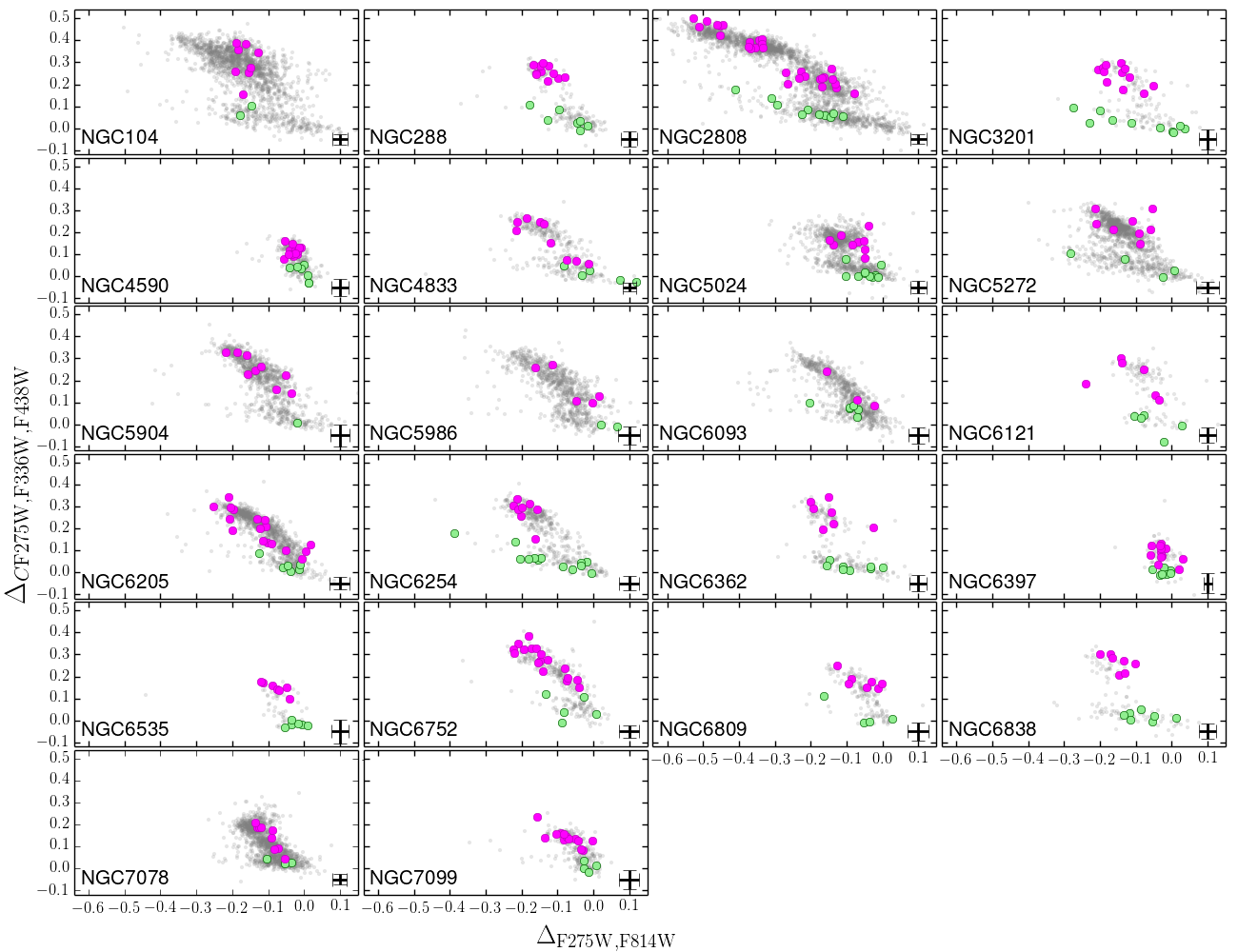
Figure 1: Reproduction of the ChM diagrams from Paper IX of the 22 analysed Type I GCs. 1G and 2G stars with available spectroscopy are marked with large green and magenta dots, respectively. Error bars are from Paper IX.

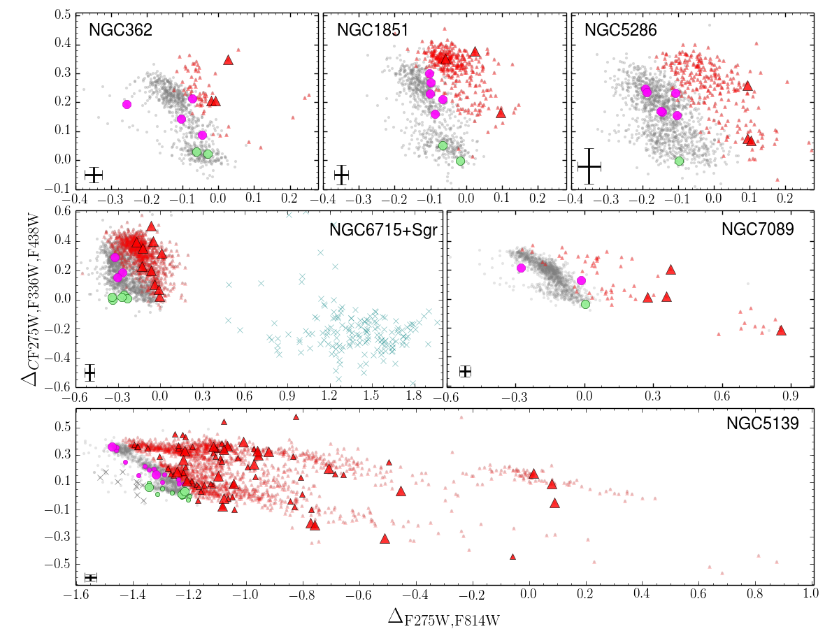
Figure 2: ChMs of the Type II GCs NGC 362, NGC 1851, NGC 5286, NGC 6715 (M 54), NGC 7089 (M 2) and NGC 5139 ($\omega$ Centauri) from Paper IX. Red-RGB stars have been represented as red triangles, while green and magenta indicate the blue-RGB 1G and 2G stars, respectively. In the ChM plane of M 54, field stars in the Sagittarius dward (Sgr) are plotted as azure crosses. For $\omega$ Centauri we have plotted both the targets from Marino et al. (2011, big symbols) and Johnson & Pilachowski (2010, small symbols); and, in addition of blue-RGB 1G and 2G stars, it is represented a third group of blue 1G stars with more negative $\Delta_{\tiny{\mathrm{F275W,F814W}}}$ that we have represented with grey crosses. The stars represented in grey crosses have not been considered in the abundance analysis of Section 3, and will be analysed in Section 4. Error bars are from Paper IX.

2.1 The spectroscopic dataset

In this work we investigate eleven chemical species, namely Li, N, O, Na, Mg, Al, Si, K, Ca, Fe, and Ba, that are among the most-commonly analysed in GCs studies. Each element has been taken into account only when both photometry and high-resolution spectroscopy is available for at least five stars in a given cluster. Elemental abundances have been taken from literature as listed in Table 1 which provides, for each cluster, the number of stars for which the chemical abundances of the various species were measured.

2.2 The $HST$ photometric dataset

The multiple stellar populations along the RGB have been identified by using the photometric catalogs published in Papers I and IX as part of the $HST$ UVIS Survey of Galactic GCs. Photometry has been derived from $HST$ images collected with the Wide-Field Channel of the Advanced Camera for Surveys (WFC/ACS) and the Ultraviolet and Visual Channel of the Wide-Field Camera 3 (UVIS/WFC3) as part of programs GO-11233, GO-12605, and GO-13297 (PI. G. Piotto, Paper I), and GO-10775 (PI.  A. Sarajedini, Sarajedini et al. 2007; Anderson et al. 2008), and from additional archive data (Paper I and IX). Photometry has been corrected for differential reddening as in Milone et al. (2012) and only stars that, according to their proper motions, are cluster members have been included in our study. The analysed $HST$ images cover $\sim$2.7$\times$2.7 square arcmin over the clusters central regions (see Papers I and IX for details).

For sake of clarity, we list here the definitions as from Paper IX that will be used along this paper to refer to the various stellar populations as appearing on the ChMs:

• 1G stars and 2G stars are separated by a line cutting through the minimum stellar density on the ChM. Thus, 1G stars are those located at lower $\Delta_{\tiny{C~{}\mathrm{F275W,F336W,F438W}}}$and will be represented by green dots if spectroscopic abundances are available;

• 2G stars are located on bluer $\Delta_{\tiny{\mathrm{F275W,F814W}}}$ and higher $\Delta_{\tiny{C~{}\mathrm{F275W,F336W,F438W}}}$, and will be represented by magenta dots if spectroscopic abundances are available.

These definitions will be used both for Type I and Type II GCs. In addition, for Type II GCs only, we also define:

• blue-RGB stars, those defining the main ChM 1G and 2G sequences, as observed in Type I GCs;

• red-RGB stars are the objects located on redder ChM sequences, only found in Type II GCs. Red-RGB stars for which spectroscopy is available will be represented as red triangles along the paper.

A note on the adopted naming scheme. We decided to use here the pure photometric classification of above. This is because of the variety of the multiple stellar populations phenomenon, as seen in the ChMs. As an example, from the chemical point of view, the presence of stellar populations with different metallicity and $s$-process elements content is the main distinctive feature of the Type II GCs, with available spectroscopy. However, this phenomenon looks variegate as well, as some “red-RGB” sub-populations have been observed not to be enhanced in $s$-elements (e.g. in M 2, Yong et al. 2014, and NGC 6934, Marino et al. 2018). Furthermore, many Type II GCs have a very tiny red component, that has not yet been investigated in terms of chemical abundances. So, at this stage, we prefer to keep our general naming scheme introduced in Paper IX for ChMs, Type I and II GCs, rather than adopting a more informative nomenclature based e.g.  on chemical abundances. This is to prevent assigning to all Type II GCs properties that they might not have. In the future, we may not exclude to adopt a more informative naming scheme.

Figure 1 reproduces the ChMs of 22 Type I GCs from Paper IX, where we have represented with green and magenta dots all the 1G and 2G stars, respectively, for which spectroscopy is available. A collection of ChMs in six Type II GCs, namely NGC 362, NGC 1851, NGC 5286, NGC 6715, NGC 7089, and NGC 5139 ($\omega$ Centauri), is shown in Figure 2. In these clusters, besides the common 1G and 2G groups (coloured green and magenta in analogy with what done in Type I GCs of Figure 1), we have represented in red the RGB stars located on the additional sequences, redder than the common sequence formed by 1G and 2G stars.

The distinction between blue- and red-RGB stars in Type II GCs has also been made on a classic colour-magnitude diagram (CMD), either the $m_{\rm F336W}$ vs. $m_{\rm F336W}-m_{\rm F814W}$ plot or using the $U$ vs. $U-I$ plot from ground-based photometry, as we will discuss in detail in Section 2.3. The colours and symbols used to distinguish 1G, 2G, and red-RGB stars introduced in Figures 1 and 2 will be used consistently hereafter.

As shown in the lower panel of Figure 2, $\omega$ Centauri exhibits the most-complex ChM among Type II GCs. In particular, we note two main streams of red-RGB stars with small and high values of $\Delta_{\tiny{C~{}\mathrm{F275W,F336W,F438W}}}$ that define the lower and upper envelope of the map. These features will be discussed in detail in Section 4.

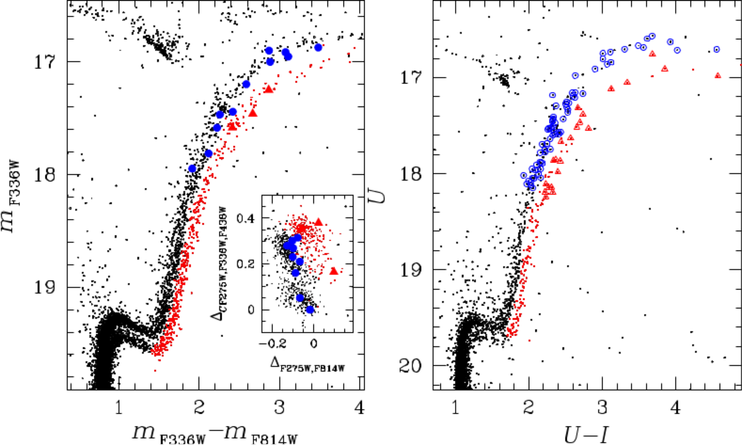
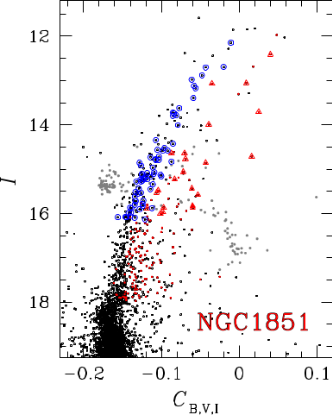
Figure 3: $m_{\rm F336W}$ vs. $m_{\rm F336W}-m_{\rm F814W}$ CMD of NGC 1851 from $HST$ photometry (left panel). The ChM is shown in the left-panel inset. Middle and right panels show the $U$ vs. $U-I$ CMD, and $I$ vs. $C_{\rm B,V,I}$ pseudo-CMD of NGC 1851 from ground-based photometry, respectively. Stars for which chemical abundances and $HST$ photometry with ChMs are available have been plotted with filled symbols: blue dots for blue-RGB stars and red triangles for the red-RGB ones. Stars with available abundances in the ground-based photometry are hereafter plotted with open symbols: blue open circles and red open triangles for blue- and red-RGBs, respectively.

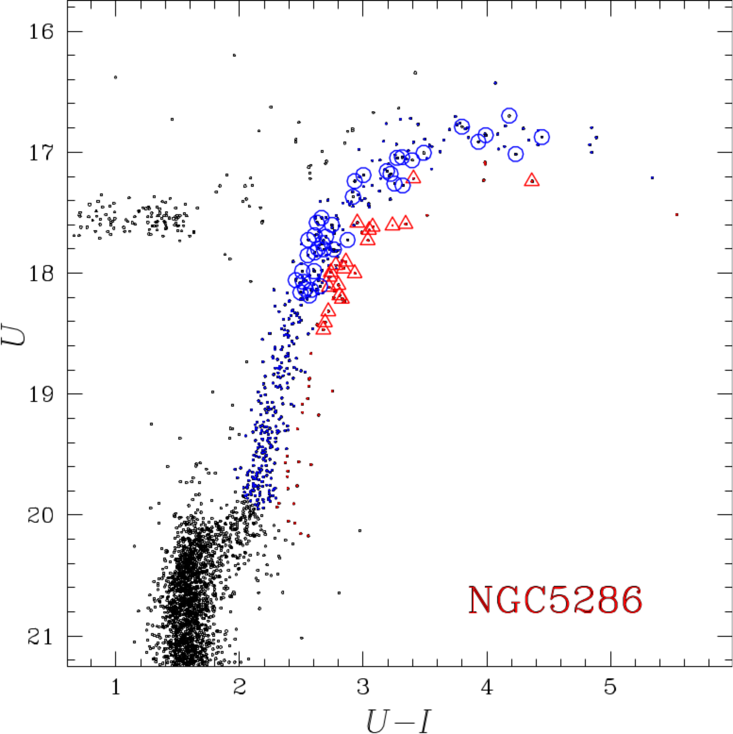
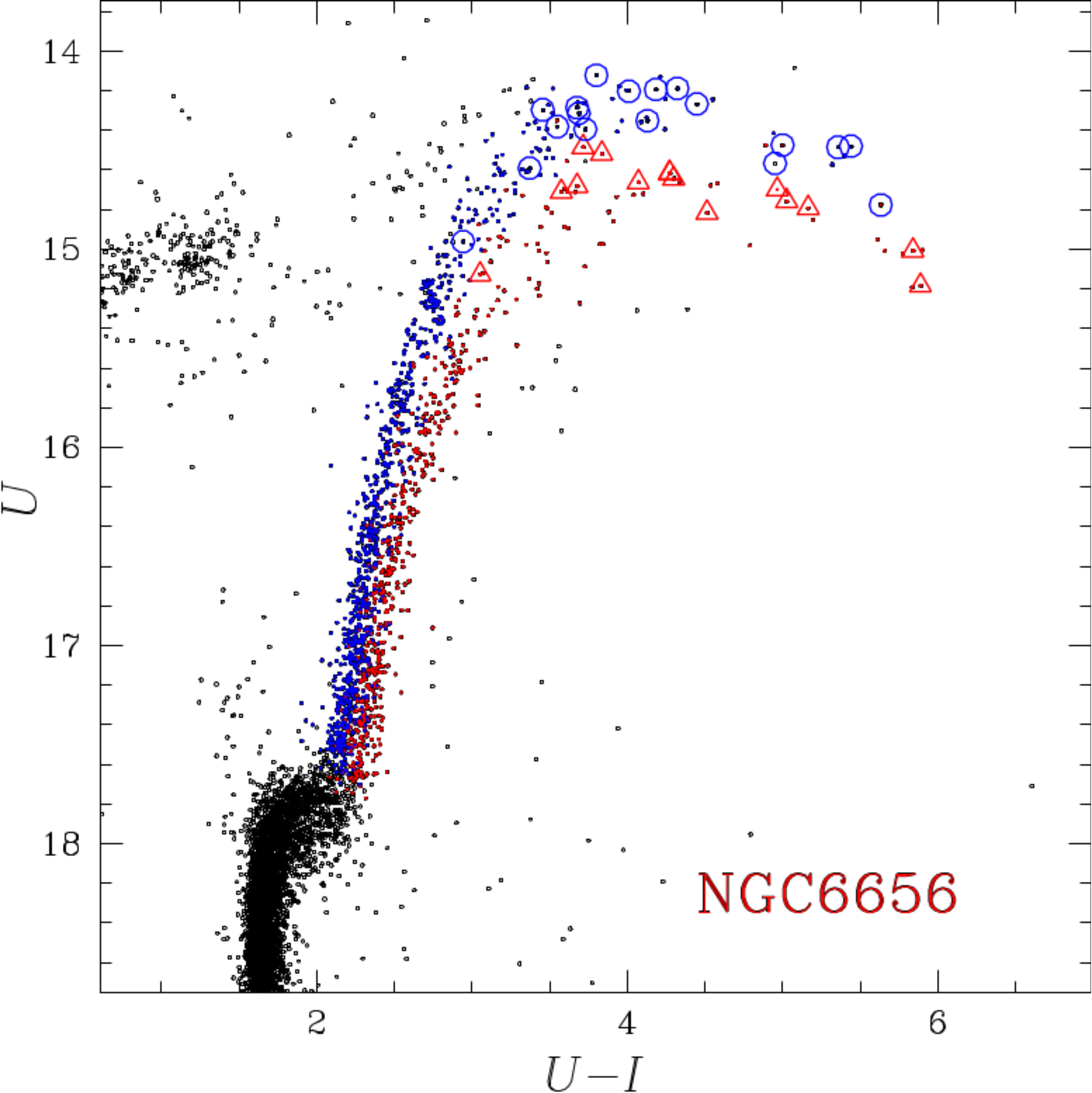
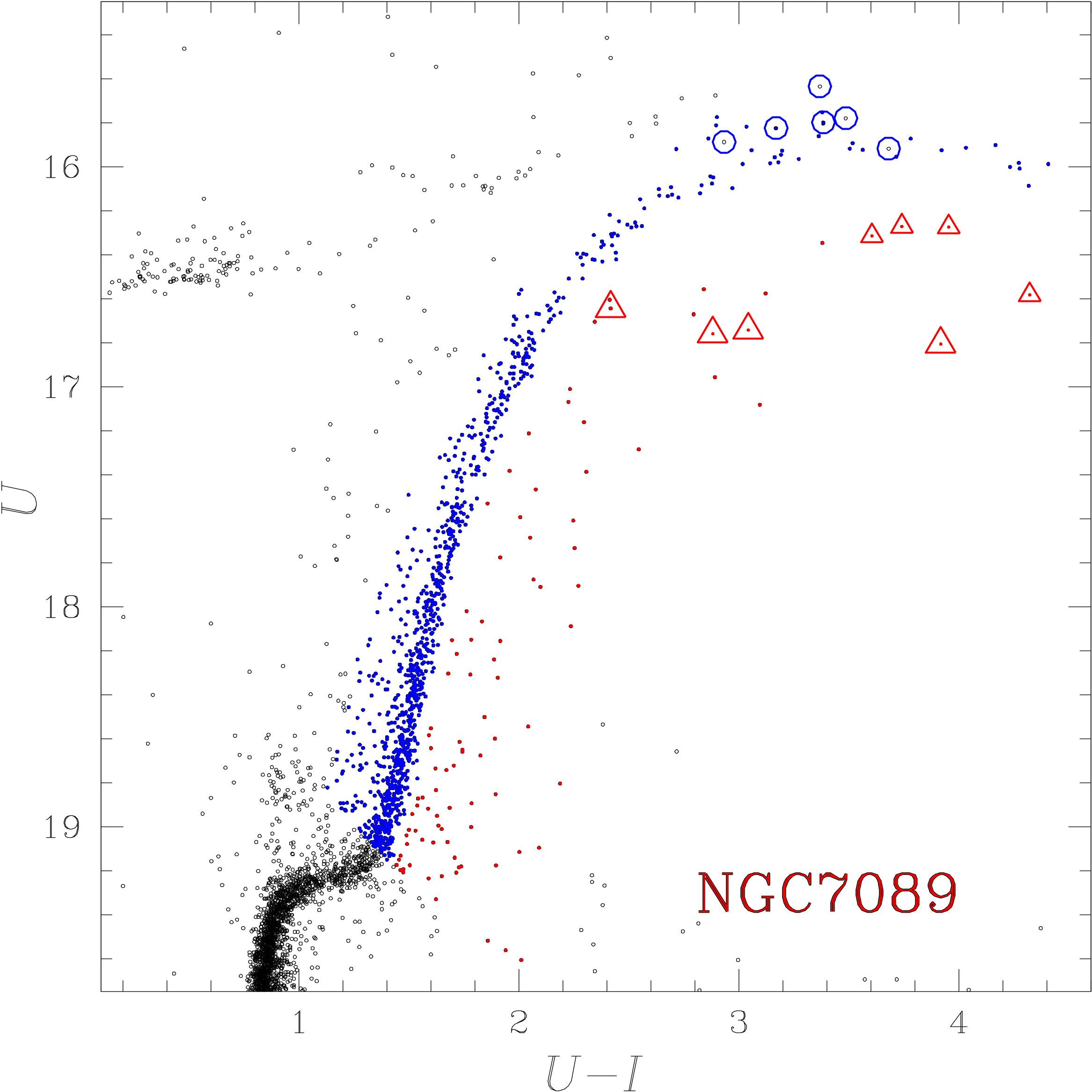
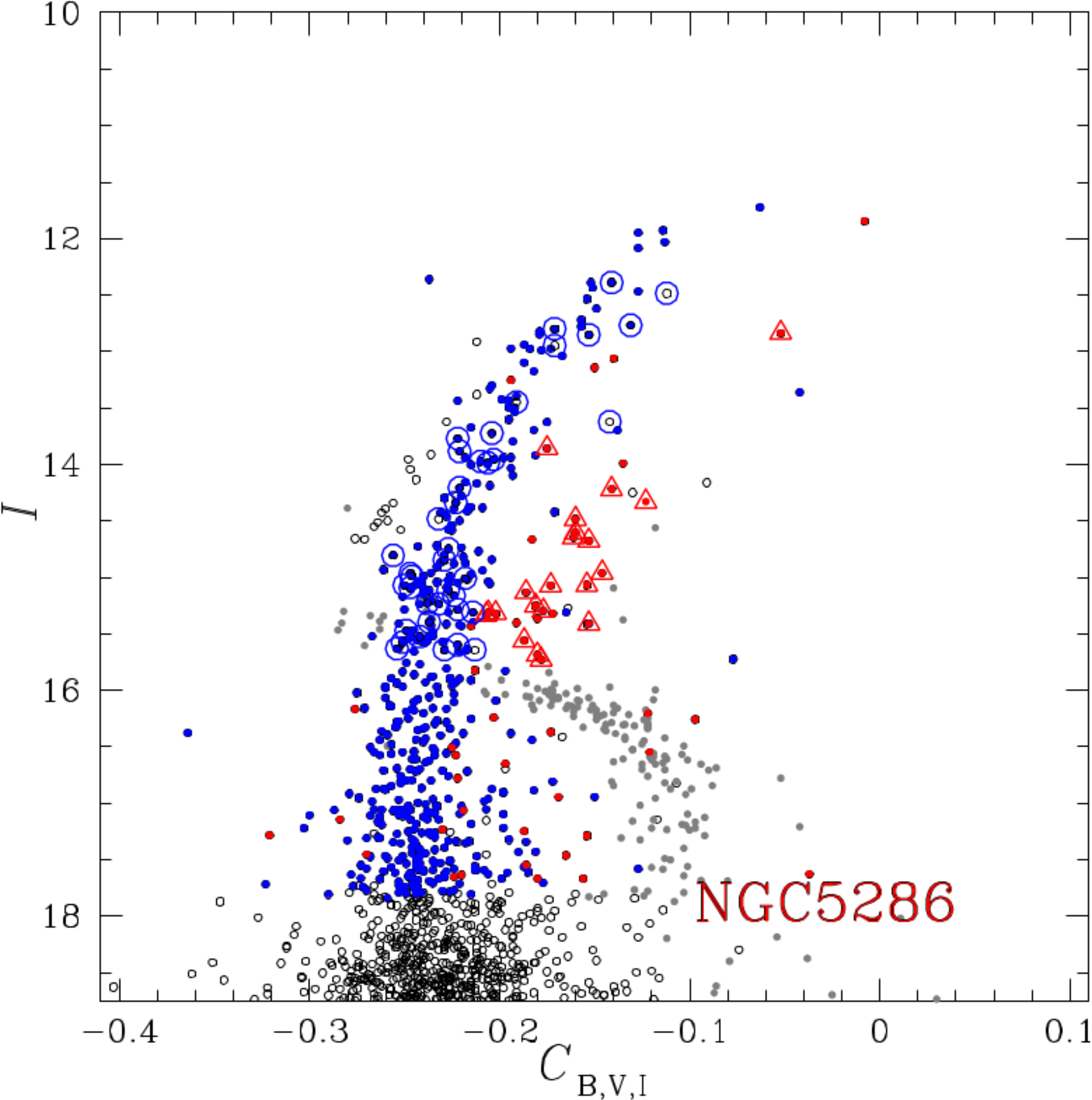
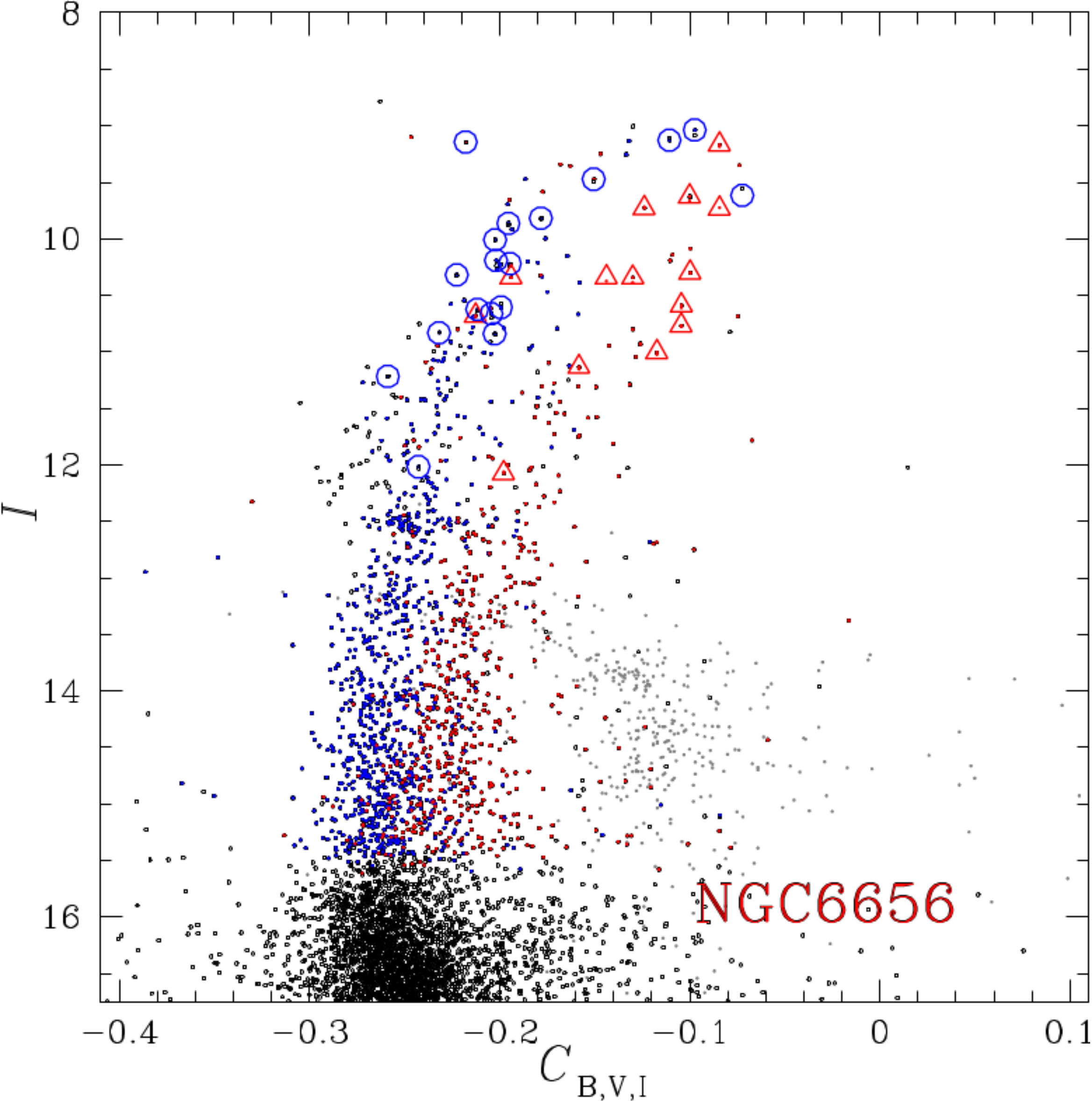
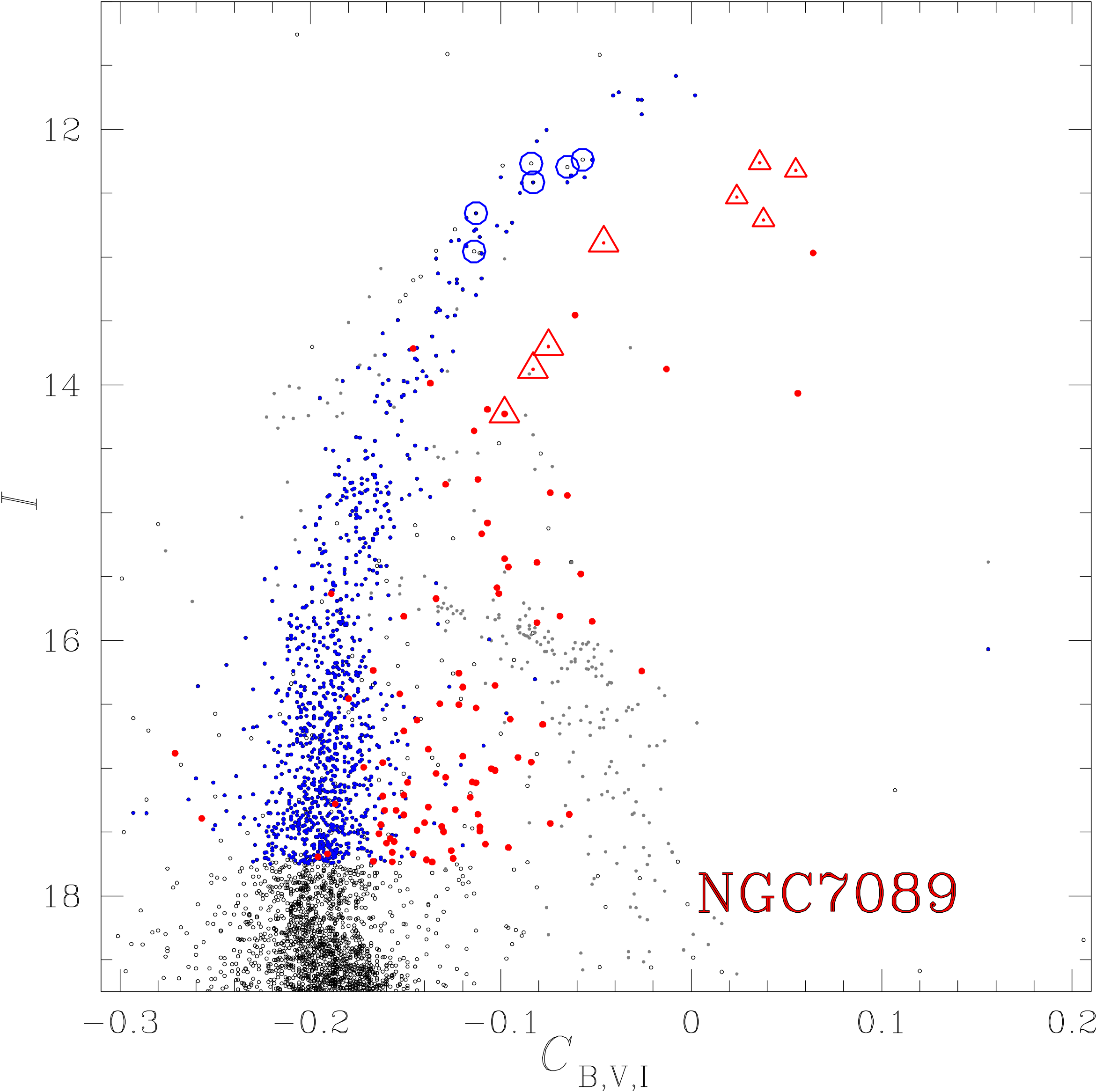
Figure 4: $U$ vs. $U-I$ CMD (upper panels) and $I$ vs. $C_{\rm B,V,I}$ pseudo CMD (bottom panels) of the Type II GCs NGC 5286, NGC 6656 (M 22) and NGC 7089 (M 2) from ground-based photometry. Red RGB stars are coloured red, while the blue points represent blue RGB stars. Spectroscopic targets are represented with red open triangles (red-RGB stars) and blue open circles (blue-RGB stars).

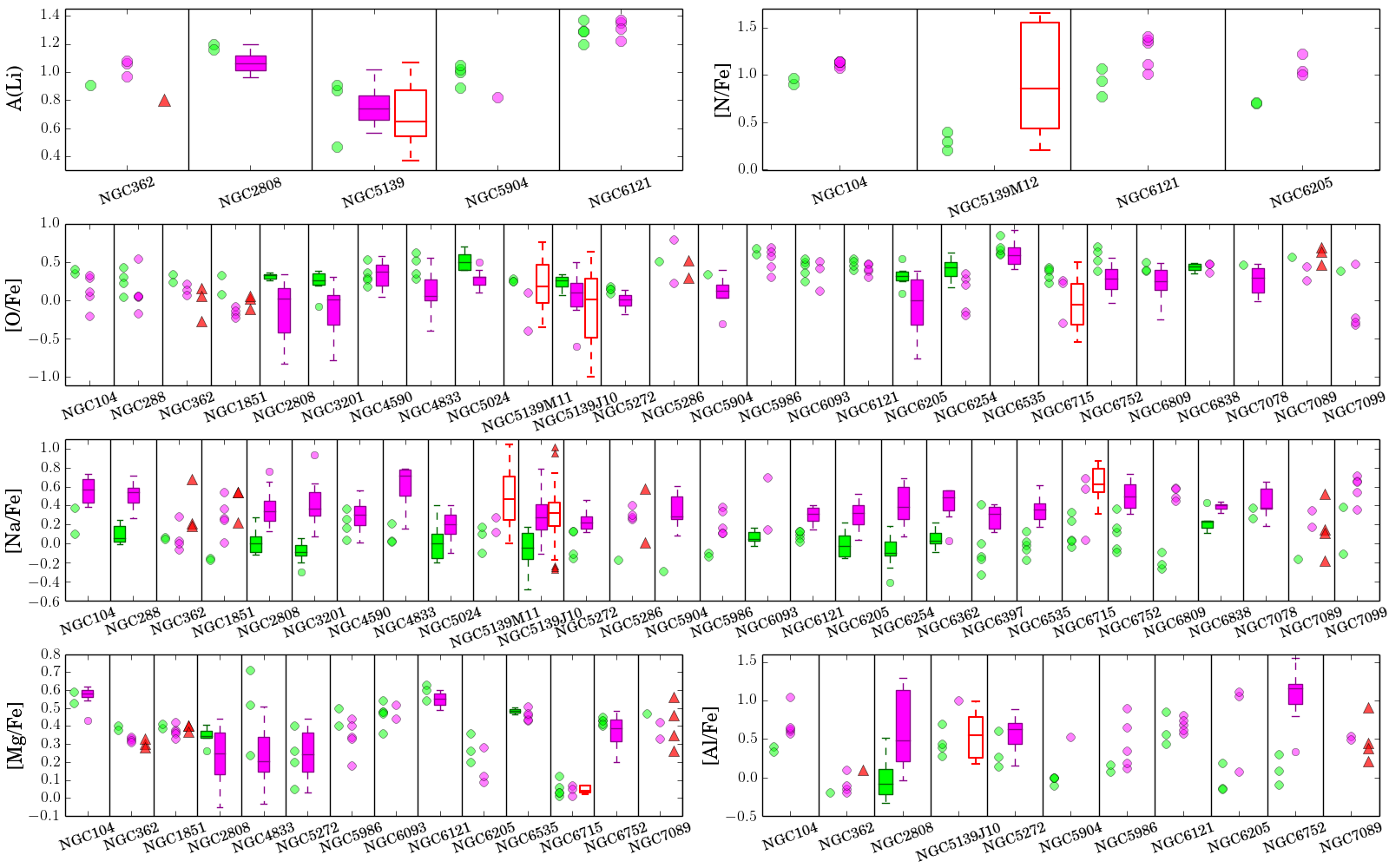
Figure 5: Box-and-whisker plot for the chemical abundances of light elements A(Li), [N/Fe], [O/Fe], [Na/Fe], [Mg/Fe], and [Al/Fe] for all the clusters analysed here. Stars selected as 1G and 2G from the ChMs are represented in green and magenta filled boxes, while stars on the red-RGB in Type II GCs have been represented in red empty boxes. Each box represents the interquartile range (IQR) of the distribution, with the median abundance marked by an horizontal line. The whiskers include observations that fall below the first quartile minus 1.5$\times$IQR or above the third quartile plus 1.5$\times$IQR. Small filled circles and triangles represent outliers or the data for 1G/2G and red-RGB stars, respectively. When less than five measurements are available for a given population, data points are represented without box-and-whisker plot.

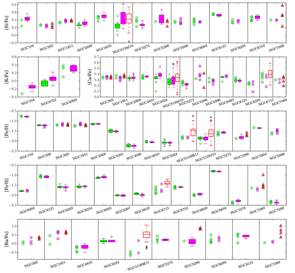
Figure 6: Same as Figure 5 for elements Si, K, Ca, Fe, and Ba.

2.3 The ground-based photometric dataset

Ground-based photometry is used here for a sub-sample of Type II GCs only, because spectroscopic chemical abundances are available for many stars lacking $HST$ observations. As discussed in Paper IX, Type II GCs are characterized by a bimodal RGB in the $m_{\rm F336W}$ vs. $m_{\rm F336W}-m_{\rm F814W}$ CMD, where the redder RGB is clearly connected with a faint sub-giant branch (SGB). As an example, the redder RGB is evident in the $m_{\rm F336W}$ vs. $m_{\rm F336W}-m_{\rm F814W}$ CMD of NGC 1851 plotted in the left panel of Figure 3 where we indicate with small red dots the red-RGB stars. Blue and red-RGB stars with available spectroscopy have been displayed with large-filled blue dots and red triangles, respectively. Clearly, stars in the blue RGB are located in the main ChM sequence, which includes 1G and 2G stars (see the inset in Figure 3), while stars in the redder RGB correspond to red-RGB stars, as defined in Section 2.2.

The middle panel of Figure 3 shows the $U$ vs. $U-I$ CMD of NGC 1851 from wide-field ground-based photometry. The split SGB and RGB are clearly visible in both CMDs, i.e., from either ground-based and $HST$ photometry. This fact is quite expected due to the similarity between $m_{\rm F336W}$ and $m_{\rm F814W}$ filters of UVIS/WFC3 and WFC/ACS and the Johnson $U$ and $I$ bands. The two main RGBs of NGC 1851 are clearly visible also in the $I$ vs. $C_{\rm B,V,I}$ pseudo-CMD, introduced by Marino et al. (2015) and shown in the right panel of Figure 3.

In the following we will thus exploit the $U$ vs. $U-I$ CMD and the $I$ vs. $C_{\rm B,V,I}$ pseudo-CMD from wide-field ground-based photometry in order to increase the sample of stars for NGC 1851, NGC 5286, and NGC 7089 for which both photometry and spectroscopy are available. Moreover, wide-field ground based photometry will allow us to extend the analysis to NGC 6656 (M 22), for which no stars with spectroscopy are available in the $HST$ field of view. Specifically, for NGC 1851, NGC 5286, and NGC 6656 we have used the photometric data collected through $U$ filter of the Wide-Field Imager (WFI) at the Max Planck 2.2m telescope at La Silla as part of the SUrvey of Multiple pOpulations in GCs (SUMO; programme 088.A-9012-A, PI. A. F. Marino). Photometry and astrometry of the WFI images have been carried out by using the method described by Anderson & King (2006). In addition, we have used $B$, $V$, $I$ photometry from the archive maintained by P. .B. Stetson (Stetson 2000).

The CMDs of NGC 5286 and NGC 6656 are strongly contaminated by field stars on the same line of sight of these two clusters. In order to select a sample of probable cluster members we have used stellar proper motions from Gaia data release 2 (DR2, Gaia collaboration et al. 2018). The $U$ vs. $U-I$ CMDs and $I$ vs. $C_{\rm B,V,I}$ pseudo-CMDs for NGC 5286, NGC 6656, and NGC 7089 are shown in Figure 4. All the stars in the ground-based CMDs of NGC 1851, NGC 5286, NGC 6656 and NGC 7089 selected as red-RGB and blue-RGB stars are coloured red and blue, respectively, with blue open circles and red open triangles representing stars with available spectroscopy.

3 The chemical composition of multiple populations over the Chromosome Maps

Figures 5 and 6 show the A(Li), [N/Fe], [O/Fe], [Na/Fe], [Mg/Fe], [Al/Fe], [Si/Fe], [K/Fe], [Ca/Fe], [Fe/H], and [Ba/Fe] abundances for all the stars in each cluster for which both spectroscopy and photometry are available. As in the previous figures, we have used green and magenta to show 1G stars and 2G stars, while red-RGB stars in Type II GCs are coloured in red. When more than five stars are available in each group, we show the box-and-whisker plot, and the median abundance. The boxes in this plot include the interquartile range (IQR) of the data, and the whiskers extend from the first quartile minus 1.5$\times$IQR to the third quartile plus 1.5$\times$IQR. The average abundances derived for each group of analysed stars, the corresponding dispersion (r.m.s.) and the number of stars that we have used are listed in Table LABEL:tab:abb.

In the following we will discuss in detail the chemical pattern observed on the various portions of the ChMs by discussing Type I and Type II GCs separately. Note that all the stars analysed here are RGB stars, as, by construction, ChMs do not include asymptotic giant branch stars (AGBs; see Paper III for a detailed description on the construction of ChMs). Our goal is to investigate the chemical elements governing the shape and variety observed on the maps for RGB stars.

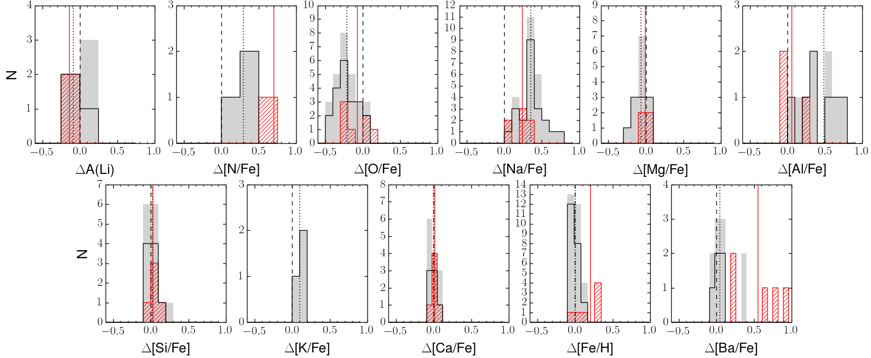
Figure 7: Distribution of the average abundance difference between 2G and 1G stars for all the analysed clusters (grey-shaded histogram) and for the Type I GCs only (black histogram). No difference is indicated by the black dashed line. Red histograms correspond to the distribution of the average abundance difference between red-RGB and blue-RGB stars in Type II GCs. The dotted black vertical line and the continuous red line indicate the mean of the difference distributions between 2G and 1G stars and red-RGB and blue-RGB stars, respectively. To better visualise the different size of variations for distinct chemical species, the range in the x axis has been kept the same for all the elements.

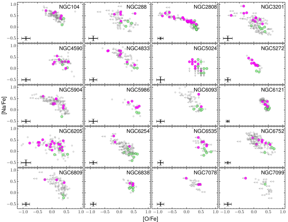
Figure 8: [Na/Fe] vs. [O/Fe] for 20 Type I clusters for which both sodium and oxygen abundances are available from literature. 1G and 2G stars are represented with large green and magenta dots, respectively. The entire sample with spectroscopic abundances is represented with grey dots. The typical error bars are taken from the reference papers listed in Table 1.

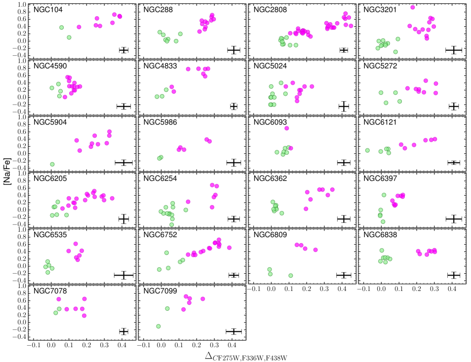
Figure 9: Sodium abundance as a function of $\Delta_{\tiny{C~{}\mathrm{F275W,F336W,F438W}}}$. 1G and 2G stars are coloured green and magenta. The typical error bars for Na are taken from the reference papers listed in Table 1. Error bars for $\Delta_{\tiny{C~{}\mathrm{F275W,F336W,F438W}}}$ are from Paper IX.

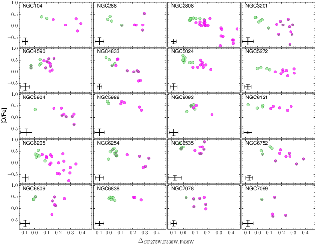
Figure 10: Oxygen abundance as a function of $\Delta_{\tiny{C~{}\mathrm{F275W,F336W,F438W}}}$. 1G and 2G stars are coloured green and magenta. Upper limits are indicated with grey downward symbols. The typical error bars for O are taken from the reference papers listed in Table 1. Error bars for $\Delta_{\tiny{C~{}\mathrm{F275W,F336W,F438W}}}$ are from Paper IX.

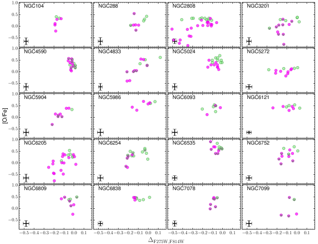
Figure 11: Oxygen abundance as a function of $\Delta_{\tiny{\mathrm{F275W,F814W}}}$. Symbols are as in Figure 10. The typical error bars for O are taken from the reference papers listed in Table 1. Error bars for $\Delta_{\tiny{\mathrm{F275W,F814W}}}$ are from Paper IX.

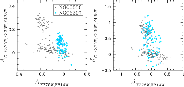
Figure 12: Left panel: Comparison of the ChMs of the two low-mass GCs NGC 6838 ([Fe/H]=$-$0.78) and NGC 6397 ([Fe/H]=$-$2.02), represented in gray dots, and azure diamonds, respectively. Right panel: Comparison of the two universal ChMs for the same clusters (see text for details). We note that the two universal ChMs almost overlap each other suggesting that the metallicity dependence of the maps has been significantly reduced in the $\delta_{\tiny{\mathrm{F275W,F814W}}}$-$\delta_{\tiny{C~{}\mathrm{F275W,F336W,F438W}}}$ plane.

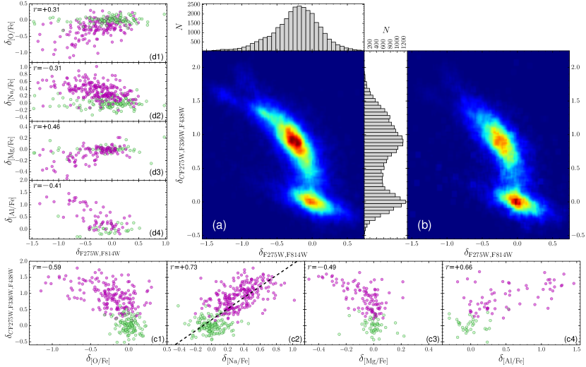
Figure 13: Panels a, b: Hess diagrams of the universal ChM for all the analysed GCs with [Fe/H]$<-0.6$. The color is indicative of the density of all the stars (panel (a)), and the stars normalised to the total number of stars in the parent cluster (panel (b)). The $\delta_{\tiny{C~{}\mathrm{F275W,F336W,F438W}}}$ and $\delta_{\tiny{\mathrm{F275W,F814W}}}$ histogram distributions for all the analyzed stars are shown as side plots of panel (a). Panels c1–c4: $\delta_{\tiny{C~{}\mathrm{F275W,F336W,F438W}}}$ vs. the abundance ratios of O, Na, Mg and Al relative to the average abundances of 1G stars. Panels d1–d4: the abundance ratios of O, Na, Mg and Al relative to the average abundances of 1G stars as a function of $\delta_{\tiny{\mathrm{F275W,F814W}}}$. In all the panels with chemical abundances 1G and 2G stars, as selected from the ChMs in Paper IX, are represented in green and magenta, respectively. For each element plot, we report the Spearman’s correlation coefficient $r$. In panel (c2) we plot the least-square fit with data (see Section 3.2 for details).

3.1 Type I GCs

As discussed in Section 2.2 the ChM of Type I GCs is composed of two main sub-structures that we have named 1G and 2G. In this section we investigate the difference in chemical content between these two stellar populations only. We start inspecting the boxplots displayed in Figures 5 and 6 from the lightest (Li) to heaviest (Ba) elements, for 1G (green) and 2G stars (magenta).

Lithium abundances plotted in Figure 5 have been corrected for departures from the LTE assumption in the cases NGC 362, NGC 2808, and $\omega$ Centauri; while for NGC 5904 and NGC 6121 (M 4) the available abundances have been derived in LTE. Note that Li has been analysed here only for stars fainter than the RGB bump, to minimise the effects of strong Li depletions that occur at this luminosity. With the exception of NGC 2808 and $\omega$ Centauri, that will be discussed in more details in Sections 3.6 and 4, all the A(Li) abundances plotted in Figure 5 are measurements, with no upper limits. No obvious difference is seen in the box-and-whisker plot of Figure 5 between the A(Li) of 1G and 2G, though very few stars are available and only in a few clusters. In the case of NGC 2808, for which we have two 1G stars and six 2G stars, the difference is $\Delta$A(Li)_2G-1G=$-$0.11$\pm$0.07, a $\sim$1.5 $\sigma$ difference, but a clearer difference can be seen when plotting Li abundances with other elements (see Section 3.6). Given the nuclear fragility of lithium one would have expected it to be strongly depleted in 2G stars, unless stars making the material for the formation of 2G stars were also making some fresh lithium (e.g., Ventura, D’Antona & Mazzitelli 2002). We note however that the lithium abundance in 2G stars depends also on the Li content of the pristine gas, with which the material ejected from whatever polluter is likely diluted (D’Antona et al. 2012).

Nitrogen abundances are available only for a few 1G and 2G stars in NGC 104 (47 Tucanae), M 4 and NGC 6205, suggesting higher N for 2G stars, as expected. In the case of $\omega$ Centauri we find that red-RGB stars span a wide range of N of more than 1 dex, and have on average higher N than 1G blue-RGB stars, but this case will be discussed more in detail in Section 3.4.

In the past years, sodium and oxygen abundances have been widely used to investigate the multiple stellar populations in several of GCs (e.g. Carretta et al. 2009). Hence, among stars studied in the Legacy Survey of GCs, sodium and oxygen abundances are available for a relatively high number of stars in 22 and 20 Type I GCs, respectively. As illustrated in Figure 5, on average 2G stars have depleted O with respect to the 1G stars in most clusters. However, the most evident differences between 1G and 2G are in the Na abundances, with the 2G having systematically higher Na, then strengthening the notion of the ChM being an optimal tool to separate GC stellar populations with different light elements chemical content.

Remarkably, the [O/Fe] distribution of 1G stars is generally consistent with typical observational errors for these spectroscopic measurements, $\sim$0.10-0.20 dex. On the other hand, when more measurements are available, 2G stars display wider oxygen spreads. Some GCs might have 1G Na distributions somewhat wider than expected from observational errors alone, e.g. NGC 5024, NGC 6752, but it is difficult to make definitive conclusions given the very small number of observed 1G objects.

No large difference is seen between the Mg abundances of 1G and 2G stars in our dataset, as plotted in Figure 5. The average Mg values of 1G and 2G stars, listed in Table LABEL:tab:abb, however suggest that there is some hint (in most cases a $\sim$1 $\sigma$ differene) for 2G stars to be Mg-depleted with respect to the 1G ones. Note indeed that for many GCs considered for Mg abundances here, Mg-Al anticorrelations have been reported in the literature (see Table 1). The GCs with the most clear enhancement in Al in 2G stars are 47 Tucanae, NGC 2808, NGC 5986, NGC 6205 and NGC 6752. Stars in the 2G of NGC 2808 show a broad Al distribution, consistent with the very extended 2G on the ChM of this GC. Only one 2G star has Al measurements available for $\omega$ Centauri and NGC 5904, and in both cases the abundance is higher than in 1G stars. Lower degree of Al enhancement is observed for NGC 5272.

Enhancements in silicon in 2G stars, linked to depletions in Mg and enrichments in Al, suggest that the temperature of the H burning generating this pattern exceeded ${T}_{6}\sim 65$ K (Arnould et al. 1999), because at this temperature the reaction ²⁷Al($p$,$\gamma$)²⁸Si becomes dominant over ²⁷Al($p$,$\alpha$)²⁴Mg. The upper panel of Figure 6 suggests that in most GCs there is no obvious evidence for Si abundance variations between 1G and 2G stars, indicating that, if present, they should be small. The exceptions are NGC 2808, where the 2G stars enriched in Al (Figure 5) have on average higher Si, and $\omega$ Centauri. Possible small Si enrichment in 2G is likely present in NGC 4833 and NGC 6752.

From Figure 6, no remarkable difference is generally observed in the elements K, Ca, Fe, and Ba between 1G and 2G. The fact that the elements shown in Figure 6 do not display any strong variation between 1G and 2G, suggests that the chemical abundances for heavier elements are not significantly involved in shaping the ChMs of Type I GCs. In general, we note that, as the 1G stars are typically a lower fraction than the 2G stars (see Paper IX), in most cases only few stars are available in this population.

To further compare the chemical composition of the different stellar populations, we have calculated for each element the difference between the average abundance of 2G and 1G stars (Table LABEL:tab:abb). The histogram distribution of such differences are represented with grey-shaded histograms for all the clusters (Type I and Type II together) in Figure 7, where we have marked the mean difference value with a black-dotted line. The corresponding distribution for Type I clusters only, is represented by the black histograms. These histograms well illustrate the chemical elements that are mostly involved in determining the distributions of stars along the ChMs, namely N, O and Na. Indeed, among the inspected species, these three elements have the highest mean difference in the chemical abundances between 1G and 2G stars, purely selected on the ChM. Still, it would be important to have far more stars with measured nitrogen, as this element is expected to show the largest differences between 1G and 2G stars and to drive much of the 1G-2G difference in the ChMs.

Thus, the ChM is a very effective tool in separating stellar populations with different light elements, as typically observed in Milky Way GCs (Papers III and XIV). The capability of ChMs to isolate stars with the typical chemical composition of different stellar populations in GCs is also illustrated in Figure 8, where we plot the 1G and 2G stars on the Na-O plane. This figure represents the Na-O anticorrelation for the 20 Type I GCs where both Na and O abundances are available on the ChMs. The grey dots show the full spectroscopic samples, whereas the large green and magenta dots represent 1G stars and 2G stars, respectively, as identified on the ChMs. As expected, 1G stars are clustered in the region of the Na-O plane with high oxygen and low sodium, while 2G stars have, on average, lower oxygen and higher sodium abundance.

The role of each element in separating stars along the $\Delta_{\tiny{\mathrm{F275W,F814W}}}$ and $\Delta_{\tiny{C~{}\mathrm{F275W,F336W,F438W}}}$ axis of the ChMs has been investigated by exploring possible correlations between the stellar abundance and the pseudo-colours $\Delta_{\tiny{\mathrm{F275W,F814W}}}$ and $\Delta_{\tiny{C~{}\mathrm{F275W,F336W,F438W}}}$. For each combination of element and pseudo-colour we have determined the statistical correlation between the two quantities by using the Spearman’s rank correlation coefficient, $r$. The corresponding uncertainty has been estimated as in Milone et al. (2014) by means of bootstrapping statistics. To do this we have generated 1,000 equal-size resamples of the original dataset by randomly sampling with replacement from the observed dataset. For each $i$-th resample, we have determined $r_{\rm i}$ and considered the 68.27^th percentile of the $r_{\rm i}$ measurements ($\sigma_{\rm r}$) as indicative of the robustness of $r$.

In Table LABEL:tab:cor we provide the derived $r$ values for the entire sample of analysed stars and for the individual groups of 1G and 2G stars. These groups have been analysed separately only when both photometry and spectroscopy are available for five stars or more. An inspection of the results listed in Table LABEL:tab:cor suggests that there is no straightforward correlation for any element with $\Delta_{\tiny{\mathrm{F275W,F814W}}}$ and $\Delta_{\tiny{C~{}\mathrm{F275W,F336W,F438W}}}$  with the exception of Na. Figure 9 reveals that in most clusters there is a strong correlation between [Na/Fe] and $\Delta_{\tiny{C~{}\mathrm{F275W,F336W,F438W}}}$ as confirmed by the Spearman’s correlation coefficients listed in Table LABEL:tab:cor. Among the clusters with the clearest Na-$\Delta_{\tiny{C~{}\mathrm{F275W,F336W,F438W}}}$ correlations, NGC 2808, NGC 5904, NGC 6205, and NGC 6752 exhibit a significant [Na/Fe]-$\Delta_{\rm F275W,F814W}$ anticorrelation with 2G stars spanning a wide range of Na. Oxygen anti-correlates with $\Delta_{\tiny{C~{}\mathrm{F275W,F336W,F438W}}}$ and correlates with $\Delta_{\tiny{\mathrm{F275W,F814W}}}$ in most GCs (see Figs. 10 and  11). Clusters with extended ChMs, and larger internal variations in He, e.g.  NGC 2808, show the most significant trends between the ChM and O abundances.

Although sodium is the element that best correlate with the ChM pattern, this does not mean that Na is the driver of 2G differences from 1G in the ChMs. Indeed, the sodium abundance itself does not directly affect any of fluxes in the passbands used to construct the maps, which instead are affected by nitrogen coming from the destruction of carbon and oxygen. So, there must be a N-Na correlations and a N-O anticorrelation, but given the sparse determinations of N, they remain to be adequately documented by spectroscopic observations for large samples of stars in each population observed in different GCs.

3.2 A universal chromosome map and relation with chemical abundances

In this Section we analyse the ChMs and chemical abundances of 1G and 2G stars, and try to envisage general patterns (if present) in the variegate zoo of ChMs, that can be valid for all the GCs. To this aim we examine here both Type I and Type II GCs, but for the latter we consider only 1G and 2G stars (i.e. only blue-RGB).

The $\Delta_{\tiny{\mathrm{F275W,F814W}}}$ and $\Delta_{\tiny{C~{}\mathrm{F275W,F336W,F438W}}}$ width of the ChM dramatically changes from one cluster to another and mainly correlates with the cluster metallicity. In particular, low-mass GCs define a narrow correlation between the ChM width and [Fe/H] (e.g. Figures 20 and 21 from Paper IX). This observational evidence is consistent with the fact that a fixed variation in helium, nitrogen, and oxygen provide smaller $m_{\rm F275W}-m_{\rm F814W}$ and $C_{\rm F275W,F336W,F438W}$ variations in metal-poor GCs than in the metal-rich ones. As an example, in the left panel of Figure 12 we compare the ChMs of NGC 6397 (azure diamonds) and NGC 6838 (gray dots), which are two low-mass GCs with metallicities [Fe/H]=$-2.02$ and [Fe/H]=$-0.78$ (Harris 1996, 2010 version). While both clusters exhibit a quite simple ChM, the $\Delta_{\tiny{\mathrm{F275W,F814W}}}$ and $\Delta_{\tiny{C~{}\mathrm{F275W,F336W,F438W}}}$ extension of stars in NGC 6838 is significantly wider than that of NGC 6397.

In an attempt to compare the ChMs of GCs with different metallicities we defined for each cluster the quantities:

$$\mbox{$\delta_{\tiny{\mathrm{F275W,F814W}}}$}=\frac{\mbox{$\Delta_{\tiny{\mathrm{F275W,F814W}}}$}-\mbox{$\Delta_{\tiny{\mathrm{F275W,F814W}}}$}^{\rm 1G,0}}{D1}$$ (1)

where $\Delta_{\tiny{\mathrm{F275W,F814W}}}$^1G,0 is the median value of $\Delta_{\tiny{\mathrm{F275W,F814W}}}$ for 1G stars, and $D1=$0.14$\times$[Fe/H]$+$0.44 is the straight line that provides the best fit of GCs with $M_{\rm V}<-7.3$ in the $\Delta_{\tiny{\mathrm{F275W,F814W}}}$ vs. [Fe/H] plane, and

$$\mbox{$\delta_{\tiny{C~{}\mathrm{F275W,F336W,F438W}}}$}=\frac{\mbox{$\Delta_{\tiny{C~{}\mathrm{F275W,F336W,F438W}}}$}-\mbox{$\Delta_{\tiny{C~{}\mathrm{F275W,F336W,F438W}}}$}^{\rm 1G,0}}{D2}$$ (2)

where $\Delta_{\tiny{C~{}\mathrm{F275W,F336W,F438W}}}$^1G,0 is the median value of $\Delta_{\tiny{C~{}\mathrm{F275W,F336W,F438W}}}$ of 1G stars, and $D2=$0.03$\times$[Fe/H]${}^{2}+$0.21$\times$[Fe/H]$+$0.43 is the square linear function that provides the best fit of GCs with $M_{\rm V}<-7.3$ in the $C_{\rm F275W,F336W,F438W}$ vs. [Fe/H] plane.

The resulting $\delta_{\tiny{C~{}\mathrm{F275W,F336W,F438W}}}$ vs. $\delta_{\tiny{\mathrm{F275W,F814W}}}$ plots of NGC 6397 and NGC 6838 RGB stars in shown in the right panel of Figure 12 and reveals that these normalised ChMs almost overlap each other. This fact suggests that the dependence on metallicity of the classical ChM is significantly reduced in this plane.

Now, that the metallicity-dependance has been reduced, we can compare the ChMs for all the clusters in our sample on the $\delta_{\tiny{\mathrm{F275W,F814W}}}$-$\delta_{\tiny{C~{}\mathrm{F275W,F336W,F438W}}}$ plane, and obtain an universal ChM. The result of this comparison is shown in Figure 13. The $\delta_{\tiny{C~{}\mathrm{F275W,F336W,F438W}}}$ vs. $\delta_{\tiny{\mathrm{F275W,F814W}}}$ Hess diagram for all GCs with [Fe/H]$<-0.6$ is plotted in panel (a), where we also show the $\delta_{\tiny{C~{}\mathrm{F275W,F336W,F438W}}}$ and $\delta_{\tiny{\mathrm{F275W,F814W}}}$ histogram distributions for all the analyzed stars. The Hess diagram plotted in the panel (b) is derived in such a way that the stars of each GC have been normalized to the total number of stars in that cluster.

These universal maps are useful tools to investigate the global properties of the multiple stellar populations phenomenon in GCs. Noticeably:

• two major overdensities are observed on the $\delta_{\tiny{C~{}\mathrm{F275W,F336W,F438W}}}$-$\delta_{\tiny{\mathrm{F275W,F814W}}}$ plane;

• a clear separation between 1G and 2G stars exists that corresponds to $\delta_{\tiny{C~{}\mathrm{F275W,F336W,F438W}}}$$\sim 0.25$;

• as expected the first overdensity corresponds to the 1G population, which appears to occupy a relatively narrow range in $\delta_{\tiny{C~{}\mathrm{F275W,F336W,F438W}}}$. The extension in $\delta_{\tiny{\mathrm{F275W,F814W}}}$ is larger, but most stars are located within $-$0.3$\lesssim$$\delta_{\tiny{\mathrm{F275W,F814W}}}$$\lesssim+$0.3;

• the bulk of 2G stars are clustered around $\delta_{\tiny{C~{}\mathrm{F275W,F336W,F438W}}}$$\sim 0.9$ with a poorly-populated tail of stars extended towards larger values of $\delta_{\tiny{C~{}\mathrm{F275W,F336W,F438W}}}$. This suggests that even if the ChMs is variegate, the dominant 2G in GCs has similar properties.

The universal ChM allows us to investigate the global variations in light elements in the overall sample of analysed GCs, in the $\delta_{\tiny{\mathrm{F275W,F814W}}}$-$\delta_{\tiny{C~{}\mathrm{F275W,F336W,F438W}}}$ plane. Panels (c1)–(c4) of Figure 13 represent $\delta_{\tiny{C~{}\mathrm{F275W,F336W,F438W}}}$ as a function of the O, Na, Mg, and Al abundance ratios relative to the average abundances of 1G stars. We find significant correlation with $\delta$[Al/Fe] and $\delta$[Na/Fe]. The $\delta_{\tiny{C~{}\mathrm{F275W,F336W,F438W}}}$–$\delta$[Na/Fe] relation is well reproduced by the straight line $\delta_{\tiny{C~{}\mathrm{F275W,F336W,F438W}}}$=1.72$\times\delta$[Na/Fe]$+$0.18 that is obtained by the least-squares fit. The tight relation and the high value of the Spearman’s rank correlation coefficient ($r=+$0.73) suggests that such relation could be exploited for empirical determination of the relative sodium abundance in GCs. We also find significant anticorrelations between $\delta_{\tiny{C~{}\mathrm{F275W,F336W,F438W}}}$ and $\delta$[O/Fe] and $\delta$[Mg/Fe]. In the latter case, we note that only stars with $\delta_{\tiny{C~{}\mathrm{F275W,F336W,F438W}}}$$\gtrsim 0.8$ exhibit magnesium variations, meaning that Mg-depleted stars are located in more extreme regions of ChMs.

Panels (d1)–(d4) show the relation between $\delta_{\tiny{\mathrm{F275W,F814W}}}$ and $\delta$[O/Fe], $\delta$[Na/Fe], $\delta$[Mg/Fe] and $\delta$[Al/Fe]. In these cases the significance of the correlations is lower than for $\delta_{\tiny{C~{}\mathrm{F275W,F336W,F438W}}}$ as indicated by the Spearman’s rank correlation coefficients quoted in the figure.

3.3 Search for intrinsic abundance variations among 1G stars

Already in Paper III it was shown that 1G stars in NGC 2808 exhibit a spread in $\Delta_{\tiny{\mathrm{F275W,F814W}}}$ with two major clumps that we have named A and B. The chemical composition of the sub-population B is constrained by the abundances derived by Carretta et al. (2006) showing that these stars have the same composition of halo field stars with similar metallicities. Unfortunately, no spectroscopic measurements are available for sub-population A stars. A comparison of the appropriate synthetic spectra and the observed colours then revealed that population B is consistent with having an helium abundance $\sim$0.03 higher in mass fraction with respect to population-A stars (Paper III). Alternatively, the 1G spread in $\Delta_{\tiny{\mathrm{F275W,F814W}}}$ may be ascribed to population-A stars being enhanced in [Fe/H] and [O/Fe] by $\sim$0.1 dex with respect to population-B stars (Paper III and D’Antona et al. 2016), but having the same helium.

The wide spread in $\Delta_{\tiny{\mathrm{F275W,F814W}}}$ among Type I clusters was fully documented in Paper IX, measuring the full $\Delta_{\tiny{\mathrm{F275W,F814W}}}$ width $W^{\rm 1G}$ for all the program clusters and showing that it mildly correlates with the cluster mass, and can reach up to $\sim 0.3$ mag in some clusters being negligibly small in others. Moreover, the 1G width $W^{\rm 1G}$ mildly correlates with the 2G width $W^{\rm 2G}$ as well, and in several cases it even exceeds it.

The discovery that even 1G stars do not represent a chemically homogeneous population has further complicated, if possible, the already puzzling phenomenon of multiple stellar populations in GCs. The helium abundance differences among both 1G and 2G stars has then been thoroughly investigated in Paper XVI, where it was shown that, if the 1G width is entirely due to a helium spread then the helium variations among 1G stars changes dramatically from one cluster to another, ranging from $\delta Y^{\rm 1G}\simeq 0$ to $\sim 0.12$, with an average $<\!\delta Y^{\rm 1G}\!>\simeq 0.05$. However, we have been unable to find a process that would enrich material in helium without a concomitant production of nitrogen at the expenses of carbon and oxygen (Paper XIV). Thus, the alternative option of a metallicity spread among 1G stars is still on the table.

We note that the presence of a spread in iron, or oxygen or any other chemical species among 1G stars would result in a positive correlation between the $\Delta_{\tiny{\mathrm{F275W,F814W}}}$ and the abundance of these elements. Therefore, the Spearman’s rank correlation coefficients between these quantities listed in Table LABEL:tab:cor may provide further insights on the origin of the 1G spread. However, from Table LABEL:tab:cor we do not find strong evidence for positive a correlation between $\Delta_{\tiny{\mathrm{F275W,F814W}}}$ and any element abundance in the analysed GCs, with few exceptions.

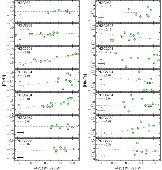
Figure 14: [Fe/H] (left panels) and sodium abundances relative to Fe (right panels) as a function of $\Delta_{\tiny{\mathrm{F275W,F814W}}}$ for the 1G stars. Only the GCs for which at least seven stars are available on the 1G region of the ChMs have been considered. In each panel, we report the Spearman correlation coefficient. The typical error bars for Na and Fe are taken from the reference papers listed in Table 1. Error bars for $\Delta_{\tiny{\mathrm{F275W,F814W}}}$ are from Paper IX.

In Figure 14 we show the [Fe/H] and [Na/Fe] abundances as a function of $\Delta_{\tiny{\mathrm{F275W,F814W}}}$ for the clusters for which data for at least seven stars are available. The $\Delta_{\tiny{\mathrm{F275W,F814W}}}$-[Fe/H] plots suggest that there is no significant correlation in five out of the seven clusters. Only in the case of NGC 3201 and NGC 6254 we have positive and significant correlations ($r\gtrsim 0.8$). The fact that NGC 3201 and NGC 6254 also exhibit a very-extended sequence of 1G makes it tempting to speculate that small internal iron variations among the 1G stars in these clusters may be responsible for the 1G spread in $\Delta_{\tiny{\mathrm{F275W,F814W}}}$. We note here that for NGC 3201 the presence of intrinsic metallicity spread has been proposed by Simmerer et al. (2013; see also Kravtsov et al. 2017). However, Mucciarelli et al. (2015) found that the RGB sample analysed in this GC does not show any evidence for intrinsic variations in Fe. An investigation of connection between a possible Fe variation and the 1G extension in $\Delta_{\tiny{\mathrm{F275W,F814W}}}$ is still undergone.

The lack of a significant trend in the other GCs suggests that iron variations, if present, are smaller and not detectable, which might also be due to the smaller range in $\Delta_{\tiny{\mathrm{F275W,F814W}}}$ (explored) in these clusters. Still, the small number of analysed 1G stars prevents us from any definitive conclusion even in the more promising cases of NGC 3201 and NGC 6254. It is also worth noting that small spurious metallicity variations can be actually be due to systematic errors in the determination of the stellar effective temperature. Indeed Carretta et al. (2009) have determined the effective temperature by assuming that all the stars have the same helium and metallicity, and projecting their stars on one single fiducial, which may not be realistic for such large variations in $\Delta_{\tiny{\mathrm{F275W,F814W}}}$.

Remarkably, the lack of any significant correlation between $\Delta_{\tiny{\mathrm{F275W,F814W}}}$ and Na abundances (right panels in Figure 14) suggests that light element abundances, likely including C, N and O, can be ruled out as the responsible for the high spread in 1G stars observed in some GCs. We conclude this section by emphasising the need to further investigate this phenomenon with chemical abundances obtained from high-resolution spectroscopy for many more stars than done so far.

Figure 15: Sodium abundance as a function of $\Delta_{\tiny{C~{}\mathrm{F275W,F336W,F438W}}}$ for a sample of Type II clusters. Blue-RGB 1G and 2G stars are represented with green and magenta dots, respectively, while red-RGB stars are plotted with red triangles, without distinguishing between the corresponding 1G and 2G. The typical error bars for Na are taken from the reference papers listed in Table 1. Error bars for $\Delta_{\tiny{C~{}\mathrm{F275W,F336W,F438W}}}$ are from Paper IX.

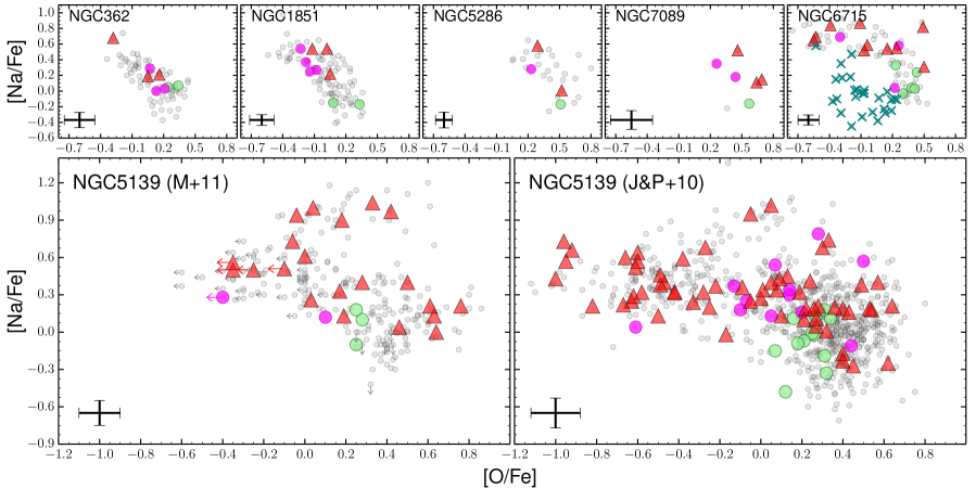
Figure 16: [Na/Fe] vs. [O/Fe] for seven Type II clusters with available abundances. The symbols are the same as in Figure 15 with blue crosses in the NGC 6715 (M 54) panel indicating stars of the Sagittarius dwarf galaxy. The typical error bars for O and Na are taken from the reference papers listed in Table 1.

3.4 Type II GCs

In addition to the 1G and 2G observed in Type I GCs, the ChMs of Type II clusters display stellar populations extending on redder colours, and distributing on a distinct red-RGB on the $m_{\rm F336W}$ vs. $m_{\rm F336W}-m_{\rm F814W}$, or $U$ vs. $(U-I)$ CMDs (Sections 2.2 and 2.3). On the chemical side, the presence of stellar populations with different metallicity and content of $s$-process elements is the main distinctive features of the “anomalous” GCs as were defined in Marino et al. (2015) from pure chemical abundance evidence. The fact that all the Type II GCs analysed spectroscopically exhibit star-to-star variations in heavy elements suggested that the class of Type II GCs, identified from photometry, corresponds to the “anomalous” GCs previously identified from spectroscopy.

In this section we explore the chemical abundances-ChMs connections for all the stellar populations observed in Type II GCs: the 1G and 2G components of the blue-RGB, corresponding to those discussed in Section 3.1 for Type I GCs, and the red-RGB populations. ChMs in Figure 2 immediately suggest that the red-RGB component includes stars at different $\Delta_{\tiny{C~{}\mathrm{F275W,F336W,F438W}}}$ implying that, similarly to the blue-RGB, it hosts both 1G and 2G stars.

From the ChMs presented in Paper IX, as well as here from Figure 2, one can see that among Type II GCs the red-RGB/blue-RGB number ratio varies considerably from cluster to cluster, whereas for most GCs the 2G stars (with higher $\Delta_{\tiny{C~{}\mathrm{F275W,F336W,F438W}}}$ values) are the dominating stellar component in the red-RGB. This sets an important constraint when trying to imagine the sequence of events that led to the two distinct (blue and red) populations in these special clusters. We now pass to discuss the chemical tagging of the various subpopulations of this group of clusters as identified on their ChMs.

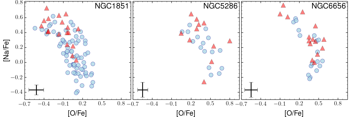
Figure 17: An expanded view of the [Na/Fe] vs. [O/Fe] anticorrelation for the clusters NGC 1851, NGC 5286 and NGC 6656 (M 22) with blue-RGB and red-RGB stars being shown as light-blue circles and red triangles, respectively. The typical error bars for O and Na are taken from the reference papers listed in Table 1 and from Marino et al. (2009, 2011) for M 22.

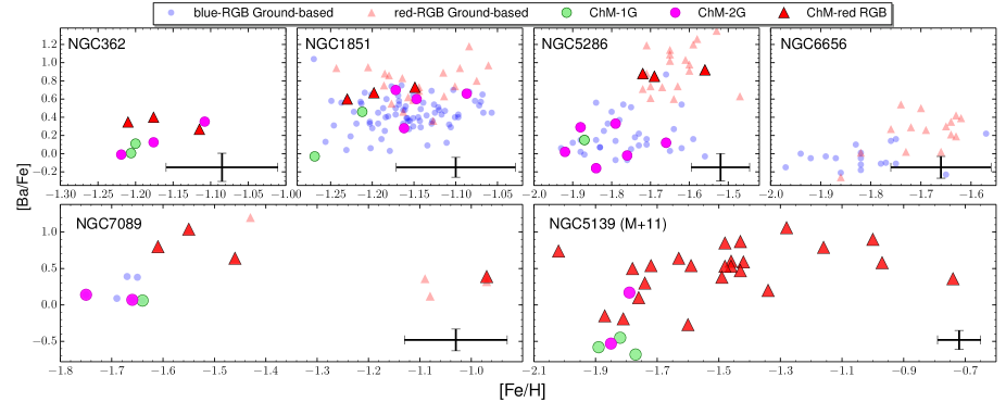
Figure 18: Barium as a function of iron abundance for Type II GCs. Symbols are as in Figure 16. For NGC 1851, NGC 5286, NGC 6656, and NGC 7089 blue and red-RGB stars with available ground-based photometry have been represented as small blue dots and red triangles, respectively. A legend of the symbols is shown on the top of the figure. The typical error bars for Fe and Ba are taken from the reference papers listed in Table 1 and from Marino et al. (2009, 2011) for M 22.

As shown in Figure 6, lithium for red-RGB stars is available only for one star in NGC 362, and 28 stars in $\omega$ Centauri. Keeping in mind that our sample includes only one star, we note that the red-RGB star in NGC 362 has lower Li than blue-RGBs. Red-RGB stars seem to have on average slightly lower Li also in $\omega$ Centauri, which will be discussed in more details in Sections 3.6 and 4.3.

Among Type II GCs, N abundances are available on the ChM only for three blue-RGB 1G stars and 13 red-RGB stars in $\omega$ Centauri. Figure 5 shows that the [N/Fe] abundances distribution in the red-RGB stars spans more than one dex, in agreement with the presence of a strong C-N anticorrelation among the stars in this cluster (e.g. Marino et al. 2012).

The same figure shows also that in $\omega$ Centauri and NGC 6715 (the Type II GCs with abundances available for a larger number of stars) the red-RGB stars have larger variations in O, and extend to higher Na abundances compared to blue-RGB stars. Although for a small number of stars, these features are observed also in the other Type II GCs plotted in Figure 5. If the large spreads in O and Na among red-RGB stars are consistent with the presence of internal anticorrelations in this stellar group (e.g. Marino et al. 2009, 2011; Johnson & Pilachowski 2010), it is noteworthy that there is a tendency of red-RGBs to have higher mean Na than blue-RGBs. In our sample we do not detect any significant difference in neither Mg nor Al between blue and red-RGB stars. We note however that Yong et al. (2014) find small increase in these elements in red-RGB stars in M 2.

From Figure 6, the typical $\alpha$ elements Si and, on a less degree, Ca appear to increase going from the blue- to the red-RGB stars in $\omega$ Centauri. This trend is seen for Si in M 2 and Ca in M 54.

Perhaps most importantly, differences are observed in the iron abundance between blue- and red-RGB stars, no matter whether belonging to the respective 1G or 2G. In $\omega$ Centauri, NGC 5286, M 54 and M 2 red-RGB stars have higher [Fe/H], as already documented in the literature (e.g. Marino et al. 2015; Carretta et al. 2010a; Yong et al. 2014). Higher Ba abundances characterise the red-RGB stars of all the Type II GCs in our sample. These results indicate that stars chemically-enriched in metallicity (Fe) and $s$-process elements have a specific location on the ChMs, which is on redder-$\Delta_{\tiny{\mathrm{F275W,F814W}}}$ 1G and 2G sequences shown in Figure 2 .

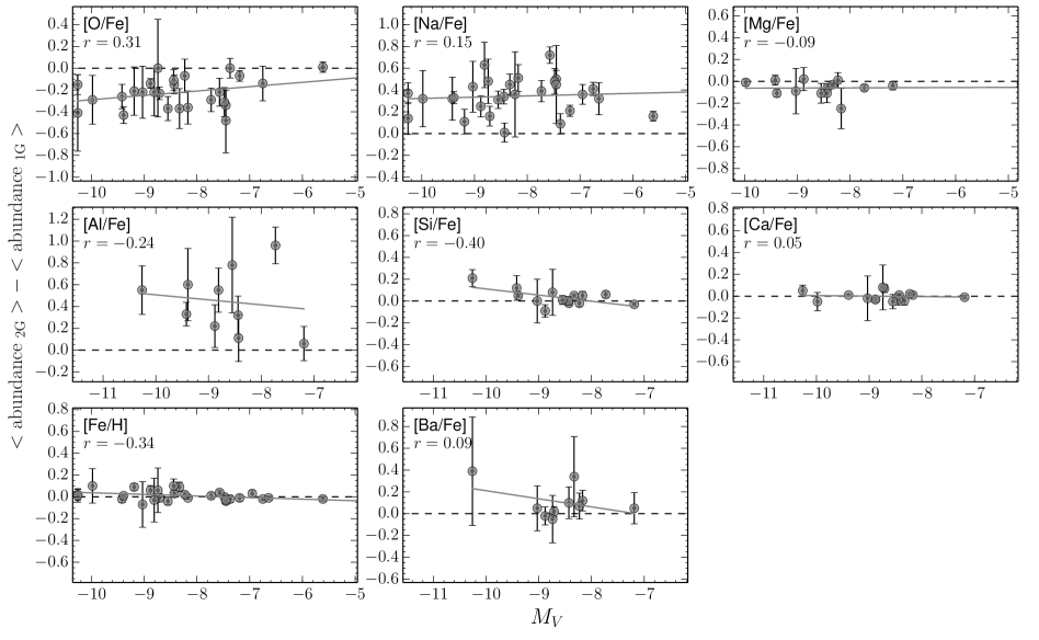
Figure 19: Abundance differences relative to Fe $<\mathrm{abundance_{\ 2G}}>-<\mathrm{abundance_{\ 1G}}>$ (and relative to H in the case of Fe) between 2G and 1G stars (from Table LABEL:tab:abb) as a function of the absolute magnitude $M_{V}$. Error bars are the square root sum of the statistical errors associated with the average values (r.m.s.$/\sqrt{(N-1)}$, with $N$ the number of measurements) of 1G and 2G stars; when only one measurement is available, the statistical error has been assumed equal to 0.20 dex. The dashed black line indicates no difference. For comparison purposes, the x and y axis have the same size in all the panels. Each panel reports the Spearman correlation coefficient $r$.

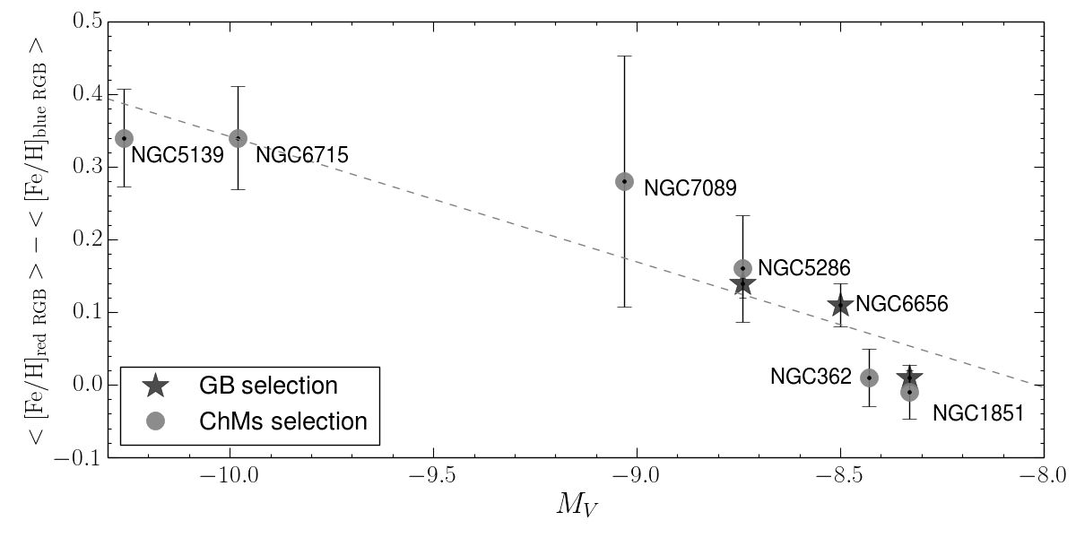
Figure 20: Differences in [Fe/H] between red and blue RGB stars as a function of the absolute magnitude for Type II GCs. The differences obtained from the ChMs selection are represented as grey-filled circles; for NGC 5286, NGC 1851, and NGC 6656 (M 22) we plot the Fe differences between the red and blue RGBs as selected from the ground-based (GB) CMDs described in Section 2.3 (star-like symbols). Error bars are the square root sum of the statistical errors associated with the average values (r.m.s.$/\sqrt{(N-1)}$, with $N$ the number of measurements) of blue and red RGB stars. The dashed grey line is the best-fit with the results obtained from the ChMs selection (grey dots), plus NGC 6656.

Similarly to what has been done for 1G and 2G components of Type I clusters (see Section 3.1), we have calculated for each element the difference between the average abundance of the red-RGB and the blue-RGB stars (lumping together the corresponding 1G and 2G) and we have plotted the distribution of such difference in Figure 7 by using red-shaded histograms. The corresponding mean differences are marked with red vertical lines. From these results, we see that blue and red-RGB stars abundance differences in Type II GCs are dominated by Fe and Ba ($s$-elements) variations.

The sodium abundances are nicely correlated with $\Delta_{\tiny{C~{}\mathrm{F275W,F336W,F438W}}}$  for both blue- and red-RGB stars, as displayed in Figure 15, just like in Type I GCs (see Figure 9). The red-RGB stars show their own internal range in $\Delta_{\tiny{C~{}\mathrm{F275W,F336W,F438W}}}$, as well as in Na, and tend to overlap with the blue-RGB 2G stars in these plots. Data plotted in Figure 15 for NGC 362, NGC 1851, NGC 5286, NGC 7089, and NGC 6715 suggest indeed that the red-RGB stars are shifted towards both slightly higher $\Delta_{\tiny{C~{}\mathrm{F275W,F336W,F438W}}}$ and Na values than blue-RGB ones.

Sodium abundances are plotted against oxygen abundances in Figure 16. Blue- and red-RGB stars do not appear to segregate from each others in these plots, emphasising that these elements are not responsible for the splitting of the ChMs of these clusters. As a general trend, 1G and 2G stars (no matter whether blue or red) are located on the Na-poor/O-rich and on the Na-rich/O-poor regions, respectively. Similarly to blue-RGB stars, red-RGB ones exhibit their own Na-O anticorrelation.

For completeness, together with the Type II GC M 54 (NGC 6715), we show in Figure 16 the stars belonging to the Sagittarius dwarf galaxy (the likely host of M 54), as identified by Carretta et al. (2010a) from their position in the CMD. While most of these stars are clustered around ([O/Fe];[Na/Fe])$\sim$($-0.1$;$-0.2$) we note a few stars with higher sodium and, possibly, lower oxygen may be present. However, there is no strong evidence for the Sagittarius stars exhibiting the 1G/2G dichotomy which is ubiquitous among GCs. Unfortunately the available data do not allow us to decide whether the few stars with high [Na/Fe] values are either contaminants from NGC 6715 stars, or spectroscopic errors, or if a small fraction of Na-rich (2G-like) stars is also present in this dwarf galaxy.

The Na-O anticorrelation of RGB stars in $\omega$ Centauri is shown in the lower panels of Figure 16 (Marino et al. 2011b, left panel and Johnson & Pilachowski 2010, right panel). Similar to Type I GCs, blue-RGB 1G stars have high O and low Na abundance and 2G stars are enhanced in Na and depleted in O; and, similarly to the other Type II GCs, red-RGB stars define their own Na-O anticorrelation. Furthermore, as previously noted, it appears that red-RGB stars have, on average, slightly higher Na abundance than blue-RGB stars. Data are consistent with a Na-O anticorrelation for red-RGB stars largely overlapping with that of blue-RGB stars, slightly extended towards higher Na, a pattern that can be recognised also in some upper panels of Figure 16. The extreme ChM of this cluster displays the presence of well-extended red streams which will be discussed in further details in Section 4.

For NGC 1851, NGC 5286, and NGC 6656 we took advantage of ground-based photometry (Section 2.3) to increase our sample of blue- and red-RGB stars from the CMDs of Figure 4, and plotted them in Figure 17. The figure confirms that blue- and red-RGB stars follow basically the same Na-O anticorrelation, with a slight predominance of low-O and high-Na in red RGB stars, in particular in NGC 1851.

The majority of Type II GCs that have been properly studied spectroscopically exhibit internal metallicity variations, with NGC 362 and NGC 1851 being possible exceptions (Carretta et al. 2013; Villanova et al. 2010). Iron abundance has been investigated in 26 clusters studied in Papers I and IX, including six Type II GCs. [Fe/H] is also available for blue- and red-RGB stars identified by using ground-based photometry in four Type II GCs including NGC 6656 for which there are no stars with jointly available spectroscopy and ChM photometry. We find that red-RGB stars are significantly enhanced in iron with respect to the remaining RGB stars in most Type II GCs and the average iron difference ranges from $\sim$0.15 dex for NGC 5286 to $\sim 1$ dex for $\omega$ Centauri. In NGC 362 and NGC 1851 there appears to be no appreciable iron difference between red- and blue-RGB stars. However, we note that the absence of a significant difference between the [Fe/H] of red and blue RGB stars in NGC 1851 (found here and by Lardo et al. 2012) appears to be at odd with the Gratton et al. (2012) finding that the faint SGB stars of this cluster are more-metal rich than those on the bright SGB. Clearly, whether a small metallicity difference exists in this cluster (and in NGC 362) between the blue- and the red-RGB stars is yet to be firmly established.

As barium is the most commonly studied $s$-process element in GCs, it has been taken as representative of this group of chemical species. Red-RGB stars are significantly enhanced in Ba with respect to blue-RGB stars. This is illustrated in Figure 18 where we plot [Ba/Fe] as a function of [Fe/H] for six Type II GCs. These results confirm that stars enhanced in both iron and barium populate the red-RGB of NGC 6656 and NGC 5286 (Marino et al. 2009, 2011a, 2015). Moreover, Figure 18 shows that stars of NGC 5286, NGC 6656, NGC 7089 and $\omega$ Centauri follow similar patters in the [Ba/Fe] vs. [Fe/H] plane as early suggested by Da Costa & Marino (2011) and Marino (2017) for the NGC 6656-$\omega$ Centauri pair.

The connection between iron and $s$-process elements seems more controversial for NGC 1851. Similarly, NGC 362 apparently does not follow the [Ba/Fe] vs. [Fe/H] trend observed in other Type II GCs.

The evidence presented in this section definitively demonstrates that Type II GCs identified from photometry correspond to the class of “anomalous” GCs that were spectroscopically identified (Marino et al. 2009; 2015). The evidence that blue- and red-RGB correspond to stars with different abundance of heavy elements is consistent with previous findings that the $s$-rich and $s$-poor stars in “anomalous” GCs host stars with different light-element abundance (Marino et al. 2009, 2011a, 2015; Carretta et al. 2010b; Yong et al. 2014).

All in all, these facts demonstrate that ChMs offer an efficient tool to identify GCs with intrinsic heavy-elements variations.

3.5 Relations with the parameters of the host GC

Having measured the mean chemical abundances for 1G and 2G stars as identified on the ChMs, we have investigated their relations with GCs’ metallicity and absolute magnitude M_V. To this aim, we derived the Spearman’s correlation coefficient between the average difference in chemical abundances between 2G and 1G ($<\mathrm{abundance_{\ 2G}}>-<\mathrm{abundance_{\ 1G}}>$) and the cluster [Fe/H] and luminosity (M_V, a proxy for the cluster mass). The results indicate that no strong correlation exists neither with [Fe/H] nor with M_V, as shown in Figure 19 for M_V and the chemical species for which data exist for more than five clusters (both Type I and Type II).

To investigate possible correlations that might be present for Type II GCs, we have derived the average metallicity difference $\Delta$([Fe/H])$=<$[Fe/H]${}_{\rm blue-RGB}-$[Fe/H]${}_{\rm red-RGB}>$ between blue and red RGB stars in each cluster. Again, this quantity does not distinguish between 1G and 2G stars, but lumps together, separately, all blue- and red-RGB stars. This selection is blind towards the various stellar populations with different Fe that could be present on distinct red RGBs. As an example, at least in $\omega$ Centauri and NGC 7089 there are more than one stellar population with enhanced Fe, defining different red RGB sequences. This translates into larger statistical errors associated with the $\Delta$([Fe/H]) of those GCs. Furthermore, our $\Delta$([Fe/H]) values hide the real range in Fe in Type II GCs, and can be observationally biased, depending on how many stars are available in each population with different Fe (see Table 1).

Having in mind all these possible shortcomings, we plot in Figure 20 the $\Delta$([Fe/H]) as a function of M_V. Interestingly, there is a quite strong correlation, with Spearman’s coefficient $r>$0.9. If confirmed, this relation would imply that more massive Type II GCs have been able to retain some material ejected by supernovae and formed stellar populations with enhanced Fe abundances. The obvious caveat is that the samples of measured stars in each cluster is rather small. For example, if we add to the current sample NGC 6934 (Marino et al. 2018), which has not been included in this study because only four stars have been observed spectroscopically, we get a point at $\Delta$([Fe/H])$=$0.20 dex and M${}_{V}=-$7.45, virtually wiping out the correlation. Of course, the present M_V of this cluster gives just an estimate of its current mass, which could be very different from the mass at birth.

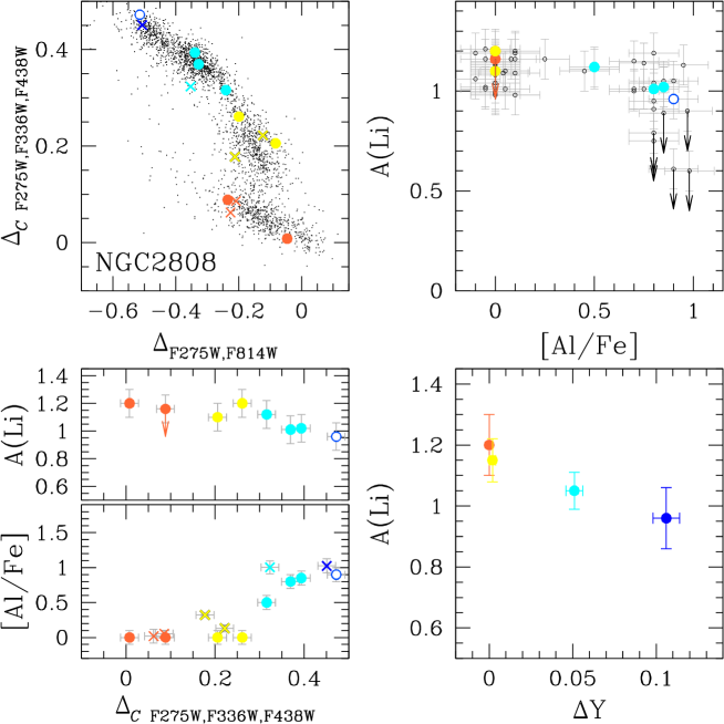
Figure 21: Upper-left panel: Reproduction of the ChM of NGC 2808 from Paper IX. Spectroscopic targets studied by D’Orazi et al. (2015) and Carretta (2014) of the populations B, C, D, and E defined in Paper III have been marked with large orange, yellow, cyan, and blue dots and crosses, respectively. These colours have been used consistently in the other panels of this figure. Upper-right panel: A(Li) vs. [Al/Fe] from D’Orazi et al. (2015). Lower-left panel: A(Li) and [Al/Fe] as a function of $\Delta_{\tiny{C~{}\mathrm{F275W,F336W,F438W}}}$, while in the lower-right panel we plot the average lithium abundance as a function of the average relative helium content of populations B–E.

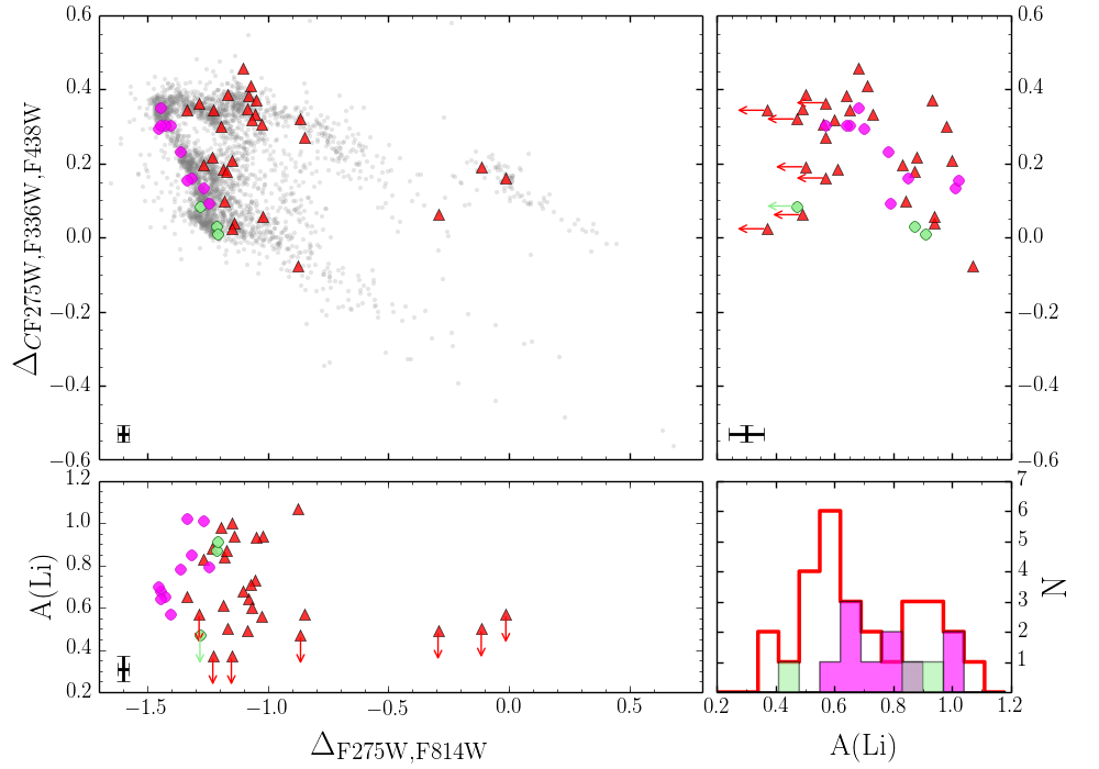
Figure 22: In the upper-left panel small grey dots represent the ChM of $\omega$ Centauri. Stars represented with large coloured symbols are those with available Li abundances (or upper limits) from Mucciarelli et al. (2018). As in Figure 2, red-RGB stars have been represented as red triangles, while green and magenta indicate the blue-RGB 1G and 2G stars. Lithium abundances as a function of $\Delta_{\tiny{\mathrm{F275W,F814W}}}$, and $\Delta_{\tiny{C~{}\mathrm{F275W,F336W,F438W}}}$ are represented on the bottom and right-side panels, respectively. The bottom-right panel is the histogram distribution of the Li abundaces for 1G (green), 2G (magenta) and red-RGB stars (red), respectively.

3.6 Lithium

Although Li can provide important constraints to the formation mechanisms of multiple stellar populations in GCs, as it is easily destroyed by proton-capture in stellar environments, its observed abundance depends on the interplay between several mechanisms that can decrease the internal and surface Li content of low-mass stars at different phases of their evolution. A drop in the surface Li abundance is observed in the subgiant branch, as a consequence of the Li dilution due to the first dredge-up, and at the luminosity of the RGB bump (Lind et al. 2009) when thermohaline mixing occurs (Charbonnel & Zahn 2007).

All the stars discussed in this section are RGBs less-luminous that the RGB bump, such that their abundances have not been affected by the strong drop due to the occurrance of thermohaline mixing. However, the Li content observed in these stars is depleted with respect to their primordial abundances.

The Li abundance in the five clusters with measurements ranges from A(Li)$\sim 0.4$ to $\sim 1.4$ (see Figure 5), with no obvious differences between 1G and 2G stars. This compares to a typical value $\sim 1$ for RGB stars having experienced the full first dredge up but not having reached yet the RGB bump level (Lind et al. 2009).

NGC 2808 hosts stellar populations with extreme photometric and spectroscopic properties (e.g. Piotto et al. 2007; Carretta et al. 2006) and provides an ideal case to investigate the lithium content of stellar populations with very different chemical composition. In Paper III we have analysed the ChM of NGC 2808 and we have identified at least five stellar populations, namely A–E with different helium and light element abundances. Specifically, population A and B have nitrogen and oxygen abundance consistent with halo field stars with the same metallicity and correspond to 1G stars, while populations C, D, and E are enhanced in sodium, depleted in oxygen and correspond to the second generation.

Lithium and aluminum abundances have been determined from spectroscopy by D’Orazi et al. (2014) for stars in four of the stellar populations identified in Paper III. These stars are marked with coloured large dots in the ChM plotted in the upper-left panel of Figure 21 while in the upper-right panel we show lithium as a function of the aluminum abundances. These plots reveal that for the available stars the lithium abundance changes only slightly from one population to another, with the population-E star being depleted in lithium by only $\sim$0.2 dex with respect to population-B stars. Note that a few stars with high Al abundance, but without any ChM information, have lower Li, including some upper limits (see D’Antona et al. 2019, for a discussion).

The slight descrease of A(Li) as a function of $\Delta_{\tiny{C~{}\mathrm{F275W,F336W,F438W}}}$ is evident from the lower-left panels of Figure 21. This figure also shows that population-D and -E stars with large $\Delta_{\tiny{C~{}\mathrm{F275W,F336W,F438W}}}$ cluster around distinct high values of [Al/Fe]. Similarly, as shown in Figure 9, population-E, which has the highest $\Delta_{\tiny{C~{}\mathrm{F275W,F336W,F438W}}}$ values, also has higher Na abundances. We note that the group of stars with high aluminum abundance (populations-D and E) host both stars with higher Li and stars with slightly lower abundances, suggesting that these populations, at least population-D, might not be chemically homogeneous. Unfortunately, the small sample with available ChM information does not allow us to make stronger conclusions.

Finally, in the lower-right panel of Figure 21 we have plotted the average lithium abundance of population B, C, D and E stars against the relative helium enhancement as derived in Paper III. The presence of stars with extreme helium abundance but only slightly Li-depleted (population E) is a challenge for scenarios that aim to explain the formation of multiple stellar populations in GCs. Indeed, under normal circumstances, depleting O and enhancing Na and Al requires very high temperatures, such that Li is totally destroyed, unless the “Cameron” Li production process is in operation, such as e.g., in massive AGB stars (Ventura et al. 2002).

In Figure 22 we report the stars with available Li abundances (from Mucciarelli et al. 2018) on the ChM of $\omega$ Centauri. Similarly to previous figures, 1G and 2G stars in the blue-RGB are plotted green and magenta dots, respectively; red-RGB stars are plotted as red triangles. The Li abundance distribution for the three stellar groups (lower-right panel) suggests a wide range for 2G stars. Two out of three 1G stars have among the highest Li in the sample, while the other one, which has the highest $\Delta_{\tiny{C~{}\mathrm{F275W,F336W,F438W}}}$ and lowest $\Delta_{\tiny{\mathrm{F275W,F814W}}}$ among 1G stars, has low Li (A(Li)$\lesssim$0.5). Lithium for 2G stars decreases with $\Delta_{\tiny{\mathrm{F275W,F814W}}}$ and with increasing $\Delta_{\tiny{C~{}\mathrm{F275W,F336W,F438W}}}$; however Li has been measured for all the 2G stars in our sample, suggesting that this element is detected even in the stellar atmospheres of stars with the highest $\Delta_{\tiny{C~{}\mathrm{F275W,F336W,F438W}}}$ (see the bottom-left and upper-right panels).

The red-RGB stars have a much broader distribution in Li, pointing to the coexistence of stars with relatively-high abundances, comparable to those observed in 1G stars, and stars with the lowest abundances in the sample, with many objects having only upper limits. Comparing the Li abundances for these stars with the location on the ChM it is clear that most red-RGB stars with high $\Delta_{\tiny{C~{}\mathrm{F275W,F336W,F438W}}}$ have low Li measurements or upper limits. This in turn suggests that these stars, also enriched in Na (Figure 15), formed from a highly-processed material enriched in Na, highly-depleted in O and Li, and are likely the most He enhanced stars in $\omega$ Centauri. To the best of our knowledge, only in the AGB scenario relatively high level of lithium can coexist with high oxygen-depletion (D’Antona et al. 2019).

In general, the presence of Li in 2G stars requires mixing with pristine gas if the polluters were massive stars, as such stars destroy lithium. As mentioned above, AGB stars can both produce and destroy lithium and in this regard the presence of an extreme 2G star in NGC 2808, extremely oxygen depleted but with fairly high lithium (A(Li)$\sim 1$) hints in favour of AGB polluters. Indeed, in such case one cannot appeal to mixing of massive star ejecta with pristine material, as this would have restored a high oxygen abundance. On the other hand, the presence of a Li-poor 1G star in $\omega$ Centauri (see Figure 5) remains quite puzzling.

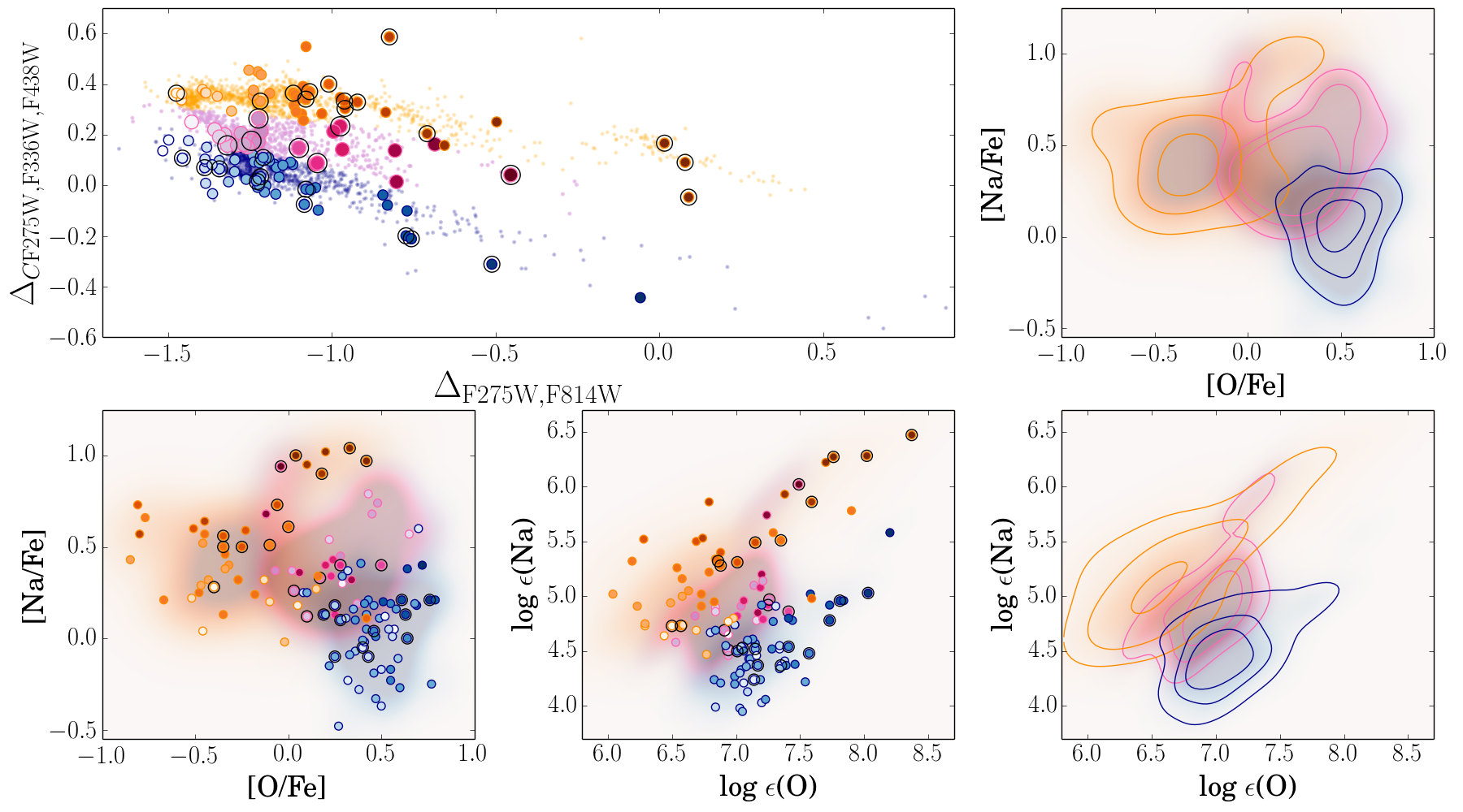
Figure 23: Chromosome map of $\omega$ Centauri (top-left panel): three main streams of stars are evident at different levels of $\Delta_{\tiny{C~{}\mathrm{F275W,F336W,F438W}}}$. The lower, middle, and upper streams have been coloured in light blue, pink and orange colours, respectively. Larger dots are stars with available chemical abundances from spectroscopy from Johnson & Pilachowski (2010, dots without the black circles) and Marino et al. (2011, black-circled points). Oxygen abundances from Johnson & Pilachowski (2010) have been shifted by $+$0.15 dex to account for the systematic difference with the O abundances inferred by Marino et al. (2011). To each star with spectroscopic data a gradient in colour has been assigned proportional to its $\Delta_{\tiny{\mathrm{F275W,F814W}}}$ value. In the lower-left and -middle panels we represent the observed Na-O anticorrelation in abundances relative to Fe (left) and in absolute abundances (middle) for the stars represented on the ChM. The two right-side panels represent the same Na-O planes with contour density levels for stars belonging to each separate stream of the map.

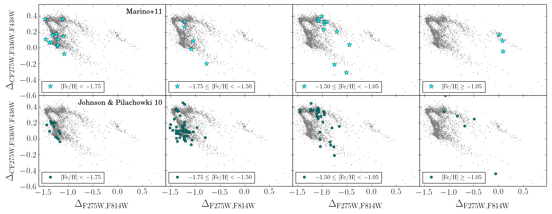
Figure 24: From the left to the right the position of stars with increasing [Fe/H] are plotted on the ChM of $\omega$ Centauri. The Marino et al. (2011) and Johnson & Pilachowski (2010) samples are plotted on the top and bottom panels, respectively. Due to the systematic Fe difference between the two samples, the Johnson & Pilachowski (2010) [Fe/H] values have been shifted by $+$0.15 dex.

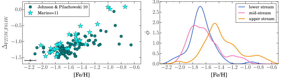
Figure 25: Left panel: $\Delta_{\tiny{\mathrm{F275W,F814W}}}$ as a function of [Fe/H] for $\omega$ Centauri. Stars in Marino et al. (2011) and Johnson & Pilachowski (2010) samples have been represented as aqua star-like symbols and teal-blue circles, respectively. Right panel: Gaussian kernel density distribution of [Fe/H] for the three streams by combining the Marino et al. (2011) and Johnson & Pilachowski (2010) samples, with the latter values increased by $+0.15$ dex to account for the systematic difference between the two datasets (see Marino et al. 2011).

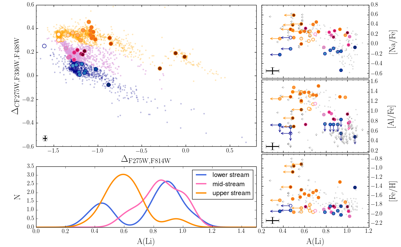
Figure 26: In the upper-left panel small grey dots represent the ChM of $\omega$ Centauri. Stars represented with large coloured symbols are those with available Li abundances (or upper limits) from Mucciarelli et al. (2018). As in Figure 23, the lower, middle, and upper streams have been coloured in light blue, pink and orange colours, respectively. To each star with spectroscopic data (large dots) a gradient in colour has been assigned proportional to its $\Delta_{\tiny{\mathrm{F275W,F814W}}}$ value. In the lower-left we represent the Gaussian kernel density distribution of Li abundances for the three streams. Right panels represent Na, Al, and Fe as a function of Li abundances (or upper limits) for all the available spectroscopic sample (small gray symbols), and the stars with ChM data (large dots), for which we used the same colour code used on the map in the upper-left panel.

4 More on the chromosome map of $\omega$ Centauri

The most complex ChM observed in the sample of clusters from the $HST$ UV Legacy Survey is that for $\omega$ Centauri (Paper IX). This complexity corresponds to a very intricate interplay of stellar populations with different chemical abundances in both light (C, N, O, Na) and heavy elements (including Fe and $s$-process elements), which is observed also on the main sequence (Bellini et al. 2017), with up to 16 distinct stellar populations being identified (Paper IX). In previous sections, for comparison purposes, we treated this GC together with the other simpler ones. However, given the complexity of $\omega$ Centauri, we devote this entire section to a more careful exploration of the ChM of this cluster.

From the ChM represented in Figure 2, we have considered the blue-RGB 1G (green) and 2G (magenta) components while lumping together all the red-RGB stars as a single population. However, this selection hides a higher level of complexity of stellar populations in this remarkable cluster. Its ChM displays quite elongated red streams asking for some more effort to be done to characterise the chemical properties of stars in this diagram.

In this section we focus on these streams, so evident in the ChM of $\omega$ Centauri at different $\Delta_{\tiny{C~{}\mathrm{F275W,F336W,F438W}}}$, so that stars have been divided into three different streams. In the top-left panel of Figure 23 we represent once again the ChM of $\omega$ Centauri, with the selection of main populations considered here:

• a lower stream, with lower $\Delta_{\tiny{C~{}\mathrm{F275W,F336W,F438W}}}$, painted in light-blue;

• a mid-stream, with intermediate $\Delta_{\tiny{C~{}\mathrm{F275W,F336W,F438W}}}$, shown in pink;

• an upper stream with the highest $\Delta_{\tiny{C~{}\mathrm{F275W,F336W,F438W}}}$ values on the map, painted in orange.

These so-selected populations of stars are on top of the normal blue- and red-RGB sequences observed in all the GC maps. In the following we discuss the chemical abundances pattern on the ChM of $\omega$ Centauri focusing on its distinctive streams. We start with the Na-O anticorrelation.

4.1 Na-O anticorrelation

The position of the selected stream populations on the O-Na plane is shown in the left-lower and central-lower panels of Figure 23, where we plot both the sample from Marino et al. (2011b) and from Johnson & Pilachowski (2010), with large and small circles, respectively.

In Section 3.4, we have discussed that in $\omega$ Centauri the normal sequence stars composed of blue-RGB 1G and 2G populations define an O-Na anticorrelation, just as in Type I GCs. Most of the stars are enhanced in O, as typical of primordial composition of halo field stars. Stars with similar high O span a relatively large range in Na. We note here that the three streams on the red side of the ChM clearly occupy different locations on the O-Na anticorrelation (see Figure 23). The upper stream (orange) stars mostly occupy the section of higher Na and lower O quadrant of the O-Na plane with [O/Fe]$<$0.0 dex. Mid-stream stars mostly distribute on a intermediate location in the O-Na plane, at intermediate values of Na, without reaching too-low O values, while lower stream stars have on average lower Na than mid-stream ones, and higher O.

Stars with most extreme positions on the red side of the ChM have the highest abundances of Na, but are not the most depleted in O, with a few stars with intermediate Na ([Na/Fe]$\sim$0.2 dex) and high O ([O/Fe]$>$0.5 dex). These stars are those defining a Na-O correlation (Marino et al. 2011b; D’Antona et al. 2011). To guide the eye, shaded contour areas have been plotted on the O-Na anticorrelation planes (right panels of Figure 23) corresponding to the colours of the different streams defined on the ChM.

4.2 Iron enrichment

To investigate the role of Fe in shaping the ChM of $\omega$ Centauri, in each panel of Figure 24 we show stars in different bins of [Fe/H], both from the Marino et al. (2011b) sample (upper panels), and the Johnson & Pilachowski one (lower panels). As a general rule, stellar populations with increasing Fe populate redder and redder regions of the map. The [Fe/H]-$\Delta_{\tiny{\mathrm{F275W,F814W}}}$ correlation is well seen in the left panel of Figure 25, and agrees with the observations of the other (simpler) Type II GCs where the red RGB stars on the ChM have higher Fe, though on lower levels.

The Fe enrichment seems generally de-coupled from the light-elements processing, corroborating previous studies on less-complex Type II GCs like M 22 (Marino et al. 2009, 2011a), and previous analysis of $\omega$ Centauri (Marino et al. 2011b, 2012). By inspecting the streams, we observe in the right panel of Figure 25 that all the three streams have a wide distribution in [Fe/H]. Interestingly, the lower and mid-streams are peaked at similar Fe abundances of [Fe/H]$\sim-$1.7 dex, with the mid-stream displaying a minor overdensity of stars at higher Fe ($-$1.2$\lesssim$[Fe/H]$\lesssim-$1.1 dex). The upper stream is peaked at higher Fe ([Fe/H]$\sim-$1.4 dex), and shows hints of multiple peaks, reaching the highest metallicity values observed in $\omega$ Centauri. This result may suggest that, while the Na enrichment (and O-depletion) occurs during the whole Fe enrichment phase experienced by $\omega$ Centauri, the strongest metallicity enrichments took place when the enrichment in high-temperature proton-capture products was maximum.

4.3 Lithium in the streams

Figure 26 shows again the ChM of $\omega$ Centauri, with the three streams represented in different colours, and the stars where Li abundances, or upper limits, are available from Mucciarelli et al. (2018). The Gaussian kernel density distribution of Li abundances for the three streams immediately suggests that, while the lower and mid- streams have distributions peaked around similar relatively-high Li, the upper stream has lower abundances (note that many of the Li abundances derived for the upper stream are upper limits).

Three stars in the lower stream have low Li abundances, A(Li)$\lesssim$0.5 dex, more consistent with values of the upper stream. On the other hand, the light element abundances of these stars are similar to those inferred for the remaining lower-stream stars, both in Na and Al (right panels in Figure 26). We note that, while for the other GCs analysed in this work the contamination from AGB stars in the ChMs is negligible, as they can be easily removed by inspecting classical CMDs, in the case of $\omega$ Centauri, the large spread in Fe makes it difficult to clean the ChM from AGBs, and we expect contamination from AGBs belonging to the metal-richer populations. From the lower panel of Figure 26 however all the three stars have Fe consistent with the metal-poor population of $\omega$ Centauri.

A careful inspection of the upper stream reveals that the stars with lower $\Delta_{\tiny{\mathrm{F275W,F814W}}}$, hence metal-poorer (these stars are the 2G stars discussed in previous sections, with the highest $\Delta_{\tiny{C~{}\mathrm{F275W,F336W,F438W}}}$), all have Li measurements, with A(Li)$\sim$0.7 dex. Upper limits suggesting A(Li)$\lesssim$0.6 dex occur for larger $\Delta_{\tiny{\mathrm{F275W,F814W}}}$ values. The three metal-richest stars, with the highest $\Delta_{\tiny{\mathrm{F275W,F814W}}}$, all have A(Li)$\lesssim$0.6 dex. In general, the upper stream hosts stars with higher Na and Al. Two stars have been found to have Li similar to the lower and mid- streams, but they follow the general upper-stream abundances in Na and Al.

4.4 On the helium enrichment

Our chemical analysis of the ChM of $\omega$ Centauri suggests that the upper stream hosts the most-extreme stars in terms of chemical properties. They are the most-processed in terms of light elements, with the highest Na and Al abundances, and the lowest Li and O. Although the Fe enrichment occurs in all the streams, the upper stream Fe distribution is peaked at higher Fe, and includes the Fe-richest stars of $\omega$ Centauri.

Among upper stream stars, those that in previous sections have been classified as 2G (blue-RGB), have likely born from material with a less degree of $p$-capture processing, if compared to the other upper stream stars belonging to the red-RGB. This is suggested by their less extreme abundances of Na, O, Al, and Li (see Sections 4.1-4.3). Specifically, these stars are those coloured in magenta (e.g.  in Figures 2 and 22), with the highest $\Delta_{\tiny{C~{}\mathrm{F275W,F336W,F438W}}}$ values.

The upper-stream red-RGB stars have more extreme enrichments in Na and Al, and depletions in Li and O. As stars with more extreme abundances in these elements have the highest level of He enrichment (e.g.  Paper III), the upper-stream red-RGB stars are likely the most-enhanced in helium.

Helium abundance variations in the $\omega$ Centauri sub-populations have originally been inferred from the analysis of main sequence (MS) stars, which suggested a higher He for the blue MS (e.g. Bedin et al. 2004; Norris 2004; Piotto et al. 2005; King et al. 2012). More recently, we have presented the He internal variations between 1G and 2G stars appearing in the ChM of $\omega$ Centauri, and found that the maximum He variation among blue-RGB stars (with similar [Fe/H]$\sim-$1.7) is $\delta(Y)=$0.09 (Paper XVI). This He difference is between the 1G (stars coloured in green in Figures 2 and 22) and 2G (blue-RGB) upper stream stars. This He variation is intended for the metal-poor population of $\omega$ Centauri corresponding to its blue-RGB.

Very interestingly, Milone et al. (2017b), by using optical-NIR CMDs, have identified two main stellar Populations I and II along the entire MS of $\omega$ Centauri, from the turn-off towards the hydrogen-burning limit. The two MSs are consistent with stellar populations with different metallicity, helium and light-element abundance. Specifically, MS-I corresponds to a metal-poor stellar population ([Fe/H]$\sim-$1.7) with $Y\sim$0.25 and [O/Fe]$\sim$0.30; while the MS-II hosts helium-rich stars with metallicity ranging from [Fe/H]$\sim-$1.7 to $-$1.4 dex, and lower [O/Fe]. Noticeably, to match the MS-II, the helium content required for the metal-poor isochrone, at [Fe/H]$\sim-$1.7, is $Y\sim$0.37, while a higher He, $Y\sim$0.40, is needed for the isochrone at [Fe/H]$\sim-$1.4.

This result is in line with our chemical analysis of the $\omega$ Centauri ChM, which suggests that the most He-enhanced stars are those in the red-RGB upper stream, that have the most extreme abundances in light elements. Stars in the blue-RGB, although highly-enriched in He, do not reach the extreme enhancements characterising the red-RGB upper stream stars.

5 Discussion and conclusions

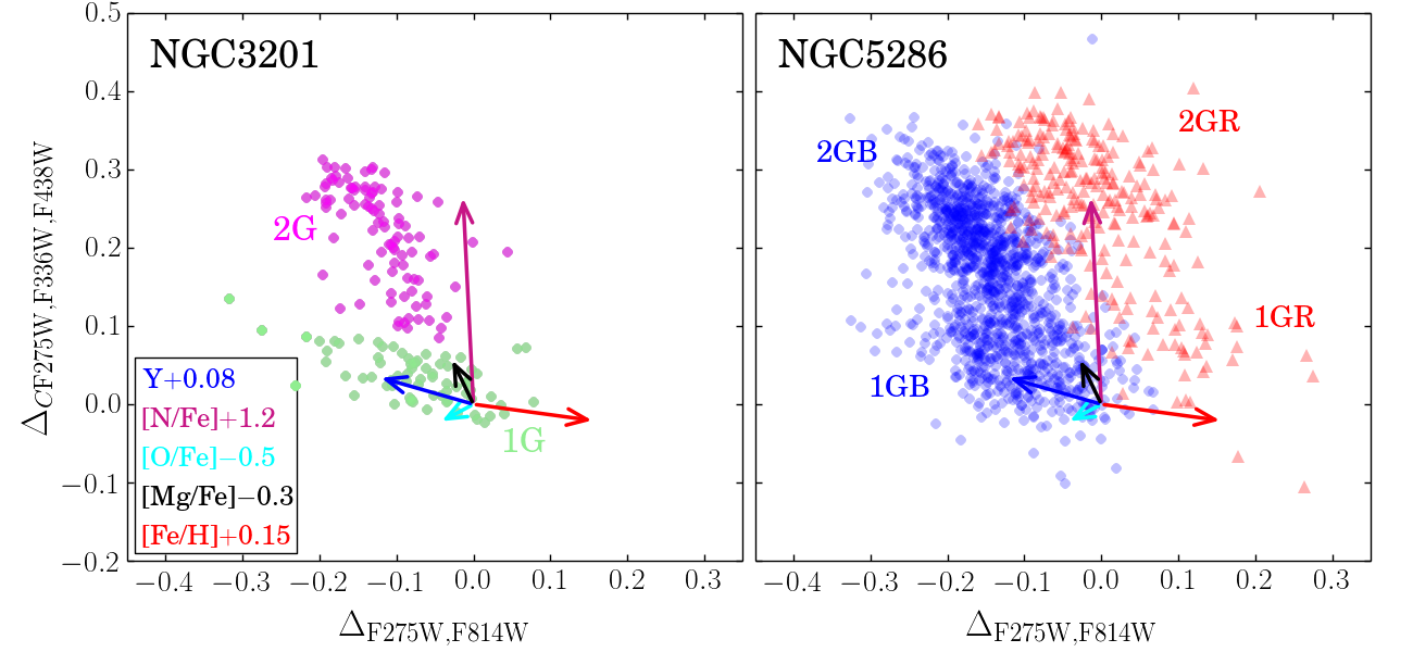
Figure 27: ChMs of the Type I GC NGC 3201 (left) and the Type II GC NGC 5286 (right). The arrows indicate the effect of changing He, C, N, Mg, and O, one a at a time by the quantities quoted in the inset, on $\Delta_{\tiny{\mathrm{F275W,F814W}}}$ and $\Delta_{\tiny{C~{}\mathrm{F275W,F336W,F438W}}}$.

Previous work, based on synthetic spectra, suggested that the chemical abundances observed among different stellar populations in Galactic GCs are strictly correlated to the distribution of stars on the ChMs (e.g. Paper XVI, see their Figure 6). This correlation has been corroborated by direct spectroscopic measurements of stars along the ChMs of a few GCs (e.g. Papers II, III, IX; Marino et al. 2017). Expanding from these early investigations, in this paper we combined the elemental abundances of Li, N, O, Na, Mg, Al, Si, K, Ca, Fe, and Ba and the ChMs of 29 GCs to characterize the chemical composition of the distinct stellar populations as identified on the ChMs, thus helping to read ChMs themselves.

Thus, we calculated the average abundance of 1G and 2G stars for each analysed element, providing the first determination –in a large sample of GCs– of the mean abundances of distinct stellar populations identified photometrically. We find strong correlations between nitrogen, oxygen and sodium abundances and the position of stars on the ChM. Specifically, 2G stars identified on the ChM, have higher N and Na and lower O than 1G stars. This was quite expected: the $\Delta_{\tiny{C~{}\mathrm{F275W,F336W,F438W}}}$ axis is highly sensitive to variations in light elements, in particular to N through absorption by NH molecules. Unfortunately, nitrogen abundances are not available for a significant number of stars and clusters, but given the known correlation between this element and Na and its anti-correlation with O, these latter elements can be used as a proxy of the N variations causing the separation of stars along the map, as proven with synthetic model atmospheres in Paper XVI. We also noticed that the lithium abundance of one extreme star in NGC 2808 (population-E) is lower, but not zero, than in the other stars, suggesting that, assumed that this highly-He enriched/highly-O depleted star formed from pure ejecta, in that material lithium was not completely destroyed.

It has emerged from previous papers of this series that two aspects of the multiple population phenomenon are particularly intriguing: it appears that even 1G stars are not chemically homogeneous, as indicated by their large spread in $\Delta_{\tiny{\mathrm{F275W,F814W}}}$, and the split of the 1G and 2G sequences in Type II GCs.

As an illustrative example, we reproduce in Figure 27 the ChMs of the Type I GC NGC 3201, with its large spread in $\Delta_{\tiny{\mathrm{F275W,F814W}}}$ among 1G stars, and the Type II GC NGC 5286, with its split 1G and 2G sequences. Overplotted on the ChMs are the vectors representing the expected changes due to the variations in He (in mass fraction Y), N, O, Mg, and Fe (C effects are almost negligible) as labelled in the left panel (see also Paper XVI). The case of NGC 3201 in Figure 27 well illustrates how variations in Fe and/or He (and possibly the C$+$N$+$O) can be responsible for variations in $\Delta_{\tiny{\mathrm{F275W,F814W}}}$. On the other hand, combined variations in helium and nitrogen are needed to populate the 2G sequence with increasing both $\Delta_{\tiny{\mathrm{F275W,F814W}}}$ and $\Delta_{\tiny{C~{}\mathrm{F275W,F336W,F438W}}}$. A mere increase in helium seems to qualitatively reproduce the distribution of 1G stars, although it remains mysterious how to produce an increase in helium without a concomitant increase in nitrogen (Paper XVI). Indeed, we find that the observed colour spread in 1G stars is not correlated to any of the analysed light elements, thus confirming that stellar populations with different chemical abundances in light elements occupy locations with different $\Delta_{\tiny{C~{}\mathrm{F275W,F336W,F438W}}}$along the 2G sequence rather than along the 1G sequence. We found only a significant correlation between $\Delta_{\tiny{\mathrm{F275W,F814W}}}$ and the iron abundance and this was in the case NGC 3201 and NGC 6254, the two clusters with the widest 1G range in $\Delta_{\tiny{\mathrm{F275W,F814W}}}$, but still too few stars with data are available even in these two clusters. Formally, the observed dispersion in iron of $\sim 0.1$ dex (see Figure14) could account for the 1G spread in NGC 3201, with iron increasing with increasing $\Delta_{\tiny{\mathrm{F275W,F814W}}}$. We conclude that a dedicated spectroscopic survey of 1G stars in many Type I GCs is required to decide whether helium or iron (or else?) are responsible for the 1G spread. This is a crucial issue to solve, in the perspective of understanding how GCs formed, along with their multiple stellar generations. If it will turn out that iron is responsible for the 1G spread, then this would imply an ongoing star formation of 1G stars while at least a few supernovae had started to pollute the interstellar medium, with 2G stars starting to form only after the 1G population was complete. Otherwise also 2G sequence would exhibit a broadening similar to that of the 1G sequence.

In Paper IX it was shown that in about 17 per cent of the analysed clusters (then called Type II GCs) the 1G and 2G sequences are split as illustrated for NGC 5286 in the right panel of Figure 27. In these clusters also the RGB splits into a blue and a red branch in e.g., the $(U-I)$ colour and this split is used to separate the two populations. It is important to emphasise that (in most clusters) there is a clear dichotomy between the blue and the red populations, as evident from Figure 27, see also Figures 3 and 4. All Type II GCs that have been analysed spectroscopically exhibit internal heavy-elements variations pointing to a connection between their unusual ChM patterns and metallicity (iron) variations. We find that the blue-RGB stars of Type II GCs behave in a very similar manner as stars Type I GCs. Stars on the red-RGB have, in most cases, higher Fe, and/or higher $s$-elements abundances. The shift on the red is likely due to a temperature effect due to an overall higher metallicity.

We have derived the average abundances of 1G and 2G stars for both blue-RGB and red-RGB populations finding no evidence for a correlation between the relative abundances of 2G and 1G stars and the absolute magnitude (a proxy of mass), nor with the metallicity of the host GCs . This result is consistent with previous findings of no correlation (or very mild correlation) between the relative average helium abundance of 2G and 1G stars and the cluster mass and metallicity (Lagioia et al. 2018; Paper XVI). On the contrary, we find a correlation between the average difference in the iron abundance of red-RGB and blue-RGB stars and the absolute luminosity of the host GC, which may suggest that the internal metallicity difference between the blue and red populations Type II GCs increases with the cluster mass. Figure 28 shows the position of various stellar systems in the half-light radius $\mathrm{(logr_{h}/pc)}$ versus absolute magnitude ($\mathrm{M_{V}}$) plane. We include the position of Milky Way GCs, classical dwarfs (DWs), Ultra Faint dwarfs (UFD), ultracompact dwarfs (UCD), dwarf-globular transition objects (DGTO) and nucleated GCs (nGC). The position of Type II GCs shows that they are in general among the most massive GCs.

The crucial question about Type II GCs is to understand what sequence of events led to formation of the blue and red populations, each with its own first and second generations. We see two possible options. A first and second generation of blue stars formed as in any other Type I cluster. The material out of which the blue 1G and 2G stars formed was almost completely converted into stars or any residual was expelled. Then the cluster re-accreted pristine gas that was enriched in iron by supernovae from the blue population (of either Type Ia or core collapse) and then formed a new 1G and its 2G companion population. Alternatively, one may think to formation within a dwarf galaxy, with the blue and red population forming at different times, while the dwarf itself was self-enriching in iron. Or even the blue and red populations formed in different places, and then merged together, as indeed speculated for NGC 1851 (Bekki & Yong 2012). Clearly the red population did not form from the gas that formed the blue 2G stars, otherwise there would be no 1G stars (i.e. nitrogen poor) in the red population.

As discussed in Paper IX, the fraction of red-RGB stars in Type II GCs varies from cluster to cluster, being NGC 6656 one of the clusters with higher fraction with $\sim$40 per cent of red-RGBs. Given the present mass of this cluster ($\sim 4\times 10^{5}\,M_{\odot}$), the metallicity of the blue population ([Fe/H]$=-1.82$) and the $\sim 0.15$ dex difference in iron abundance between its red and blue populations, we estimate that the whole red population now contains just $\sim 1.2\,M_{\odot}$ of iron more than if it had the same iron abundance of the blue population. According to current understanding, a stellar generation makes $\sim 0.5\,M_{\odot}$ of iron from core collapse supernovae every 1,000 $M_{\odot}$ of gas turned into stars (e.g., Renzini & Andreon 2014 and references therein). Hence, the blue population alone should have produced over $\sim 120\,M_{\odot}$ of iron and therefore just $\sim 1$ per cent of it would have been sufficient to enrich the red population to the observed level. Similarly, the cluster NGC 5286 has a mass of $\sim 4.6\times 10^{5}\,M_{\odot}$, $\sim$17 per cent of which in the red-RGB population, a metallicity of the blue population [Fe/H]$=-1.77$ and again a $\sim 0.15$ dex difference in iron abundance between its red and blue populations. Therefore, the same calculation leads to just $\sim 0.6\,M_{\odot}$ of excess iron in the red population, while the blue population would have produced $\sim 200\,M_{\odot}$ of iron, with only $\sim 0.3$ per cent of it being sufficient to enrich the red population to the observed level. From this point of view, there may not be such a big difference between Type I clusters that have not retained much supernova ejecta at all and those Type II clusters that have retained just a very small fraction of it. For example, the same exercise for $\omega$ Centauri indicates that only $\sim 2$ per cent of the iron from the supernovae from its metal poor population would have been sufficient to enrich its metal rich population to the observed level (Renzini et al. 2015; Renzini 2013). Thus, in this respect there appears to be no much difference between Type I clusters, that have lost 100 per cent the iron produced by their stars, and Type II clusters that have lost just $\sim 99$ per cent.

Finally, we have explored in details the ChM of $\omega$ Centauri, whose wide ranges in chemical abundances of CNONa and Fe make it an ideal laboratory to test the role of these elements in shaping the maps of GCs. We found that $\Delta_{\tiny{\mathrm{F275W,F814W}}}$ is very well correlated to [Fe/H], and that the location of the stars on the three main streams, that we have defined in the ChM, is related to a different position on the Na-O abundances plane. The upper stream is the most distinctive either in the Na-O plane, but also in terms of Fe, Li, and likely He content. There is no doubt that in this most massive GC of the MW galaxy metal enrichment and star formation from proton-capture processed material have concomitantly taken place, though still in a sequence of events that we have not yet been able to decipher from either its ChM or spectroscopic analysis. But we keep trying.

In conclusion, the $\Delta_{\tiny{\mathrm{F275W,F814W}}}$ spread among 1G stars ($W_{\rm 1G}$) can be ascribed either to a helium or to an iron spread, with a spread $\Delta Y$ giving a similar $W_{\rm 1G}$ that would be produced by a similar spread in [Fe/H], for example, an enhancement $\Delta Y=0.1$ would produce the same $W_{\rm 1G}$ than a variation $\Delta$[Fe/H]=$-$0.1. Here the minus sign indicates that the bluest 1G stars would be either helium rich of iron poor. Though giving similar results, a spread in helium of $\sim 0.1$ is much more demanding in terms of nucleosynthesis than a spread of $\sim 0.1$ dex in iron, to the point that no viable scenario could be envisaged that would produce such an helium spread without affecting the nitrogen abundance (cf. Paper XVI). For this reason we have been cautious in claiming the 1G spread being due to helium, after we first hinted at it in Paper III. We now have for two clusters, namely NGC 3201 and NGC 6254, some weak evidence supporting the notion of the 1G spread being due to iron, rather than to helium (Figure 14). However, more systematic and accurate measurements of the iron abundance in several clusters with wide 1G sequences are necessary before definitely ascribe to iron the observed spread. Iron dishomogeneities at the level of $\sim 0.1$ dex in the molecular cloud generating the 1G stars appears to be a plausible alternative to helium and could be generated by incomplete mixing of the supernova ejecta in the parent dwarf galaxy. We also notice that the correlation of the 1G spread $W_{\rm 1G}$ with cluster mass (implied by Figure 19 in Paper XVI) is also reminiscent of the Type II syndrome (multiple iron abundances) being confined to the most massive GCs, as shown in Figure 28, as if retaining supernova ejecta were more likely in the progenitors of the most massive clusters.

The chromosome maps will be available via the http://progetti.dfa.unipd.it/GALFOR/ web page and at the CDS (cdsarc.u-strasbg.fr). We will continually update the files and figures of this paper in the http://progetti.dfa.unipd.it/GALFOR/ webpage as new spectroscopic observations come in.

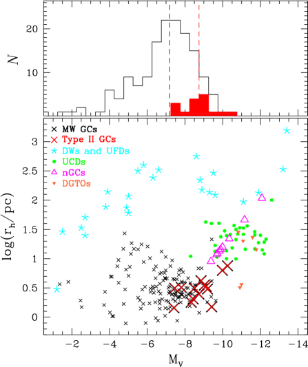
Figure 28: Absolute magnitude ($\mathrm{M_{V}}$) as a function of the half-light radius ($\mathrm{r_{h}}$). Different colours and symbols represent different class of objects: Milky Way GCs (black crosses; Harris 2010), Milky Way satellites including dwarf (DW; Irwin & Hatzidimitriou 1995; Mateo 1998), ultrafaint dwarf galaxies (UFDs) and all the objects discovered by the SDSS (Willman et al. 2005, 2006; Belokurov et al. 2006, 2007; Zucker et al. 2006; Jerjen 2010), ultracompact dwarf galaxies (UCDs; Brodie et al. 2011), nucleated GCs (nGCs; Georgiev et al. 2009), dwarf-globular transition objects (DGTOs; Haşegan et al. 2005). Type II GCs, here considered as all the objects with internal metallicity and/or heavy-elements variations, have been marked with red crosses. The upper panel is the histogram distribution of the $\mathrm{M_{V}}$ of GCs, with Type II GCs shown in red.

Table 1: Description of the spectroscopic dataset used in this paper. For each cluster and element we provide the number of stars for which both spectroscopy and $HST$ photometry is available and the reference to the spectroscopic paper.

CLUSTER	Reference	A(Li)	[N/Fe]	[O/Fe]	[Na/Fe]	[Mg/Fe]	[Al/Fe]	[Si/Fe]	[K/Fe]	[Ca/Fe]	[Fe/H]	[Ba/Fe]
NGC 104	Carretta et al. 2009	—	—	7	10	—	—	—	—	—	10	—
	Carretta et al. 2013	—	7	—	—	10	7	10	—	—	—	—
	Mucciarelli et al. 2017	—	—	—	—	—	—	—	10	—	—	—
NGC 288	Carretta et al. 2009	—	—	9	19	—	—	—	—	—	19	—
NGC 362	Carretta et al. 2013	—	—	8	9	9	—	9	—	9	9	8
	D’Orazi et al. 2015	5	—	—	—	—	6	—	—	—	—	—
NGC 1851	Carretta et al. 2010b	—	—	11	12	12	—	12	—	12	12	11
NGC 2808	Carretta 2014, 2015	—	—	32	40	40	7	40	—	39	40	—
	D’Orazi et al. 2015	8	—	—	—	—	—	—	—	—	—	—
NGC 3201	Carretta et al. 2009	—	—	16	22	—	—	—	—	—	22	—
NGC 4590	Carretta et al. 2009	—	—	15	17	—	—	—	—	—	22	—
NGC 4833	Carretta et al. 2014	—	—	14	12	12	—	15	—	15	15	15
NGC 5024	Boberg et al. 2016	—	—	19	20	—	—	—	—	20	20	20
NGC 5139	Johnson & Pilachowski 2010	—	—	94	94	—	11	92	—	94	94	—
	Marino et al. 2011b	—	—	28	32	—	—	—	—	—	32	32
	Marino et al. 2012	—	16	—	—	—	—	—	—	—	—	—
	Mucciarelli et al. 2018	42	—	—	—	—	—	—	—	—	—	—
NGC 5272	Sneden et al. 2004	—	—	12	12	12	11	12	—	12	12	12
NGC 5286	Marino et al. 2015	—	—	5	7	—	—	10	—	8	10	10
NGC 5904	Carretta et al. 2009	—	—	9	10	—	—	—	—	—	10	—
	D’Orazi et al. 2014	5	—	—	—	—	5	—	—	—	—	—
NGC 5986	Johnson et al. 2017	—	—	—	8	—	—	—	—	—	—	—
NGC 6093	Carretta et al. 2015	—	—	10	10	9	—	10	—	11	11	10
NGC 6121	Marino et al. 2008	—	—	9	11	11	9	11	—	11	11	10
	D’Orazi & Marino 2010	8	—	—	—	—	—	—	—	—	—	—
	Carretta et al. 2013	—	8	—	—	—	—	—	—	—	—	—
NGC 6205	Johnson & Pilachowski 2012	—	—	23	23	—	—	—	—	—	23	—
	Mészáros et al. 2015	—	5	—	—	6	6	6	—	6	—	—
NGC 6254	Carretta et al. 2009	—	—	15	18	—	—	—	—	—	21	—
NGC 6362	Mucciarelli et al. 2016	—	—	—	16	—	—	—	—	—	16	—
NGC 6397	Carretta et al. 2009	—	—	—	13	—	—	—	—	—	6	—
NGC 6535	Bragaglia et al. 2017	—	—	12	11	11	—	—	—	—	13	—
NGC 6715	Carretta et al. 2010a	—	—	18	18	18	—	—	—	18	18	—
NGC 6752	Carretta et al. 2009	—	—	13	21	—	—	—	—	—	23	—
	Carretta et al. 2012	—	—	—	—	19	15	22	—	—	—	—
	Mucciarelli et al. 2017	—	—	—	—	—	—	—	23	—	—	—
NGC 6809	Carretta et al. 2009	—	—	10	8	—	—	—	—	—	12	—
	Mucciarelli et al. 2017	—	—	—	—	—	—	—	11	—	—	—
NGC 6838	Carretta et al. 2009	—	—	9	14	—	—	—	—	—	14	—
NGC 7078	Carretta et al. 2009	—	—	8	9	—	—	—	—	—	13	—
NGC 7089	Yong et al. 2014	—	—	6	8	7	7	8	—	8	8	8
NGC 7099	Carretta et al. 2009	—	—	6	8	—	—	—	—	—	18	—

Table 2: For each element and GC, we provide the average abundance for 1G stars, 2G stars, blue-RGB, and red-RGB stars. The corresponding r.m.s. and the number of used stars are also listed.

		1G			2G			Blue-RGB			Red-RGB
A(Li)
NGC 0362	0.91	—	1	1.04	0.06	3	1.00	0.08	4	0.80	0.00	1
NGC 2808	1.18	0.03	2	1.07	0.09	6	1.10	0.09	8	—	—	0
NGC 5904	0.99	0.07	4	0.82	—	1	0.96	0.10	5	—	—	0
NGC 6121	1.29	0.07	4	1.31	0.07	4	1.30	0.06	8	—	—	0
[N/Fe]
NGC 0104	0.94	0.05	2	1.12	0.03	5	1.07	0.10	7	—	—	0
NGC 6121	0.93	0.15	3	1.25	0.18	5	1.13	0.23	8	—	—	0
NGC 5139 (M+12)	0.30	0.10	3	—	—	0	0.30	0.10	3	1.00	0.55	13
NGC 6205	0.71	0.01	2	1.09	0.12	3	0.93	0.22	5	—	—	0
[O/Fe]
NGC 0104	0.38	0.04	2	0.12	0.21	5	0.19	0.22	7	—	—	0
NGC 0288	0.25	0.16	4	0.11	0.26	5	0.17	0.22	9	—	—	0
NGC 0362	0.29	0.07	2	0.14	0.07	3	0.20	0.10	5	$-$0.02	0.23	3
NGC 1851	0.21	0.18	2	$-$0.16	0.06	4	$-$0.04	0.21	6	$-$0.02	0.09	3
NGC 2808	0.31	0.04	10	$-$0.12	0.34	21	0.02	0.35	31	—	—	0
NGC 3201	0.23	0.17	6	$-$0.11	0.33	10	0.02	0.32	16	—	—	0
NGC 4590	0.33	0.13	5	0.33	0.19	10	0.33	0.17	15	—	—	0
NGC 4833	0.44	0.16	4	0.08	0.34	9	0.19	0.34	13	—	—	0
NGC 5024	0.51	0.11	9	0.28	0.12	9	0.39	0.16	18	—	—	0
NGC 5139 (M+11)	0.26	0.02	3	$-$0.15	0.35	2	0.10	0.29	5	0.19	0.33	21
NGC 5139 (J+10)	0.23	0.09	12	0.08	0.29	12	0.15	0.23	24	$-$0.09	0.46	60
NGC 5272	0.14	0.04	4	$-$0.00	0.10	8	0.04	0.11	12	—	—	0
NGC 5286	0.51	—	1	0.51	0.40	2	0.51	0.28	3	0.41	0.16	2
NGC 5904	0.34	—	1	0.12	0.22	8	0.14	0.22	9	—	—	0
NGC 5986	0.64	0.06	2	0.53	0.15	5	0.56	0.14	7	—	—	0
NGC 6093	0.42	0.12	5	0.35	0.20	3	0.40	0.15	8	—	—	0
NGC 6121	0.48	0.06	4	0.41	0.07	5	0.44	0.07	9	—	—	0
NGC 6205	0.32	0.15	6	$-$0.05	0.35	17	0.05	0.35	23	—	—	0
NGC 6254	0.41	0.14	10	0.10	0.25	5	0.31	0.23	15	—	—	0
NGC 6535	0.68	0.10	5	0.61	0.18	7	0.64	0.15	12	—	—	0
NGC 6715	0.35	0.08	5	0.06	0.31	3	0.24	0.23	8	$-$0.03	0.38	10
NGC 6752	0.56	0.14	4	0.27	0.19	8	0.37	0.22	12	—	—	0
NGC 6809	0.43	0.06	3	0.21	0.27	6	0.28	0.24	9	—	—	0
NGC 6838	0.43	0.05	6	0.44	0.06	3	0.43	0.05	9	—	—	0
NGC 7078	0.47	—	1	0.26	0.21	6	0.29	0.20	7	—	—	0
NGC 7089	0.57	—	1	0.35	0.13	2	0.42	0.16	3	0.60	0.12	3
NGC 7099	0.39	—	1	$-$0.09	0.38	4	0.00	0.39	5	—	—	0
[Na/Fe]
NGC 0104	0.24	0.19	2	0.56	0.14	8	0.49	0.19	10	—	—	0
NGC 0288	0.10	0.10	7	0.51	0.14	11	0.35	0.24	18	—	—	0
NGC 0362	0.06	0.01	2	0.07	0.15	4	0.06	0.12	6	0.36	0.28	3
NGC 1851	$-$0.16	0.01	2	0.29	0.19	5	0.16	0.27	7	0.43	0.18	3
NGC 2808	0.01	0.12	10	0.37	0.16	29	0.27	0.22	39	—	—	0
NGC 3201	$-$0.09	0.10	10	0.41	0.24	12	0.18	0.31	22	—	—	0
NGC 4590	0.21	0.14	4	0.30	0.16	13	0.28	0.16	17	—	—	0
NGC 4833	0.09	0.11	3	0.60	0.25	8	0.46	0.32	11	—	—	0
NGC 5024	0.03	0.21	10	0.19	0.16	9	0.11	0.20	19	—	—	0
NGC 5139 (M+11)	0.06	0.14	3	0.20	0.11	2	0.12	0.14	5	0.49	0.31	24
NGC 5139 (J+10)	$-$0.07	0.20	12	0.30	0.25	12	0.11	0.29	24	0.32	0.26	60
NGC 5272	0.00	0.15	4	0.25	0.12	8	0.16	0.17	12	—	—	0
NGC 5286	$-$0.17	—	1	0.31	0.06	4	0.21	0.22	5	0.30	0.40	2
NGC 5904	$-$0.29	—	1	0.34	0.17	9	0.28	0.25	10	—	—	0
NGC 5986	$-$0.12	0.02	2	0.22	0.13	5	0.13	0.20	7	—	—	0
NGC 6093	0.07	0.07	6	0.43	0.39	2	0.16	0.23	8	—	—	0
NGC 6121	0.09	0.05	5	0.30	0.10	6	0.20	0.13	11	—	—	0
NGC 6205	$-$0.01	0.16	6	0.30	0.14	17	0.22	0.19	23	—	—	0
NGC 6254	$-$0.08	0.16	12	0.40	0.24	6	0.08	0.29	18	—	—	0
NGC 6362	0.05	0.10	8	0.41	0.20	7	0.22	0.24	15	—	—	0
NGC 6397	$-$0.04	0.28	5	0.28	0.12	8	0.16	0.25	13	—	—	0
NGC 6535	$-$0.02	0.11	5	0.36	0.16	6	0.19	0.24	11	—	—	0
NGC 6715	0.12	0.15	5	0.44	0.35	3	0.24	0.27	8	0.64	0.17	10
NGC 6752	0.10	0.18	5	0.49	0.14	15	0.40	0.23	20	—	—	0
NGC 6809	$-$0.19	0.09	3	0.53	0.07	4	0.22	0.39	7	—	—	0
NGC 6838	0.23	0.10	7	0.39	0.05	7	0.31	0.12	14	—	—	0
NGC 7078	0.32	0.08	2	0.43	0.18	6	0.41	0.16	8	—	—	0
NGC 7089	$-$0.16	—	1	0.27	0.12	2	0.12	0.26	3	0.15	0.29	4
NGC 7099	0.14	0.35	2	0.59	0.14	5	0.46	0.28	7	—	—	0
[Mg/Fe]
NGC 0104	0.56	0.04	2	0.57	0.06	8	0.56	0.05	10	—	—	0
NGC 0362	0.39	0.01	2	0.33	0.01	4	0.35	0.04	6	0.30	0.03	3
NGC 1851	0.40	0.01	2	0.37	0.03	5	0.38	0.03	7	0.39	0.02	3
NGC 2808	0.35	0.04	10	0.24	0.15	29	0.26	0.14	39	—	—	0
NGC 4833	0.49	0.24	3	0.24	0.19	8	0.30	0.23	11	—	—	0
NGC 5272	0.23	0.15	4	0.25	0.16	8	0.24	0.15	12	—	—	0
NGC 5986	0.45	0.07	2	0.34	0.10	5	0.37	0.10	7	—	—	0
NGC 6093	0.47	0.07	5	0.48	0.06	2	0.47	0.06	7	—	—	0
NGC 6121	0.59	0.05	3	0.55	0.04	8	0.56	0.04	11	—	—	0
NGC 6205	0.27	0.08	3	0.16	0.10	3	0.22	0.10	6	—	—	0
NGC 6535	0.48	0.01	6	0.46	0.03	5	0.47	0.02	11	—	—	0
NGC 6715	0.05	0.04	5	0.04	0.03	3	0.05	0.04	8	0.04	0.02	10
NGC 6752	0.43	0.02	5	0.37	0.09	13	0.39	0.08	18	—	—	0
NGC 7089	0.47	—	1	0.38	0.06	2	0.41	0.07	3	0.41	0.13	4
[Al/Fe]
NGC 0104	0.37	0.05	2	0.70	0.19	5	0.60	0.23	7	—	—	0
NGC 0362	$-$0.20	—	1	$-$0.09	0.13	4	$-$0.11	0.12	5	0.10	0.00	1
NGC 2808	0.20	0.28	3	0.62	0.46	4	0.44	0.43	7	—	—	0
NGC 5139 (J+10)	0.45	0.17	4	1.00	—	1	0.56	0.29	5	0.54	0.32	7
NGC 5272	0.34	0.24	3	0.56	0.26	8	0.50	0.26	11	—	—	0
NGC 5904	$-$0.03	0.05	4	0.52	—	1	0.08	0.25	5	—	—	0
NGC 5986	0.12	0.06	2	0.44	0.33	5	0.35	0.31	7	—	—	0
NGC 6121	0.62	0.21	3	0.68	0.10	5	0.66	0.14	8	—	—	0
NGC 6205	$-$0.03	0.19	3	0.75	0.59	3	0.36	0.58	6	—	—	0
NGC 6752	0.10	0.19	3	1.06	0.32	11	0.86	0.50	14	—	—	0
NGC 7089	—	—	0	0.52	0.04	2	0.52	0.04	2	0.49	0.30	4
[Si/Fe]
NGC 0104	0.32	0.11	2	0.44	0.07	8	0.42	0.09	10	—	—	0
NGC 0362	0.27	0.00	2	0.25	0.03	4	0.26	0.02	6	0.26	0.06	3
NGC 1851	0.33	0.01	2	0.38	0.02	5	0.37	0.03	7	0.39	0.02	3
NGC 2808	0.26	0.03	10	0.31	0.05	29	0.30	0.05	39	—	—	0
NGC 4833	0.45	0.06	5	0.50	0.07	9	0.48	0.07	14	—	—	0
NGC 5139 (J+10)	0.24	0.13	11	0.45	0.22	12	0.35	0.20	23	0.43	0.18	59
NGC 5272	0.36	0.09	4	0.27	0.06	8	0.30	0.08	12	—	—	0
NGC 5286	0.36	—	1	0.44	0.15	6	0.43	0.14	7	0.33	0.08	3
NGC 5986	0.35	0.03	2	0.35	0.06	5	0.35	0.05	7	—	—	0
NGC 6093	0.37	0.06	5	0.35	0.01	3	0.36	0.05	8	—	—	0
NGC 6121	0.55	0.02	3	0.52	0.03	8	0.53	0.03	11	—	—	0
NGC 6205	0.36	0.05	3	0.37	0.03	3	0.36	0.04	6	—	—	0
NGC 6752	0.42	0.05	5	0.48	0.05	16	0.46	0.05	21	—	—	0
NGC 7089	0.40	—	1	0.40	0.01	2	0.40	0.01	3	0.52	0.22	4
[K/Fe]
NGC  0104	$-$0.32	—	1	$-$0.16	0.07	9	$-$0.17	0.08	10	—	—	0
NGC  6752	$-$0.06	0.07	8	0.05	0.09	13	0.02	0.10	21	—	—	0
NGC  6809	0.27	0.15	3	0.30	0.09	7	0.29	0.09	10	—	—	0
[Ca/Fe]
NGC 0362	0.34	0.01	2	0.35	0.02	4	0.35	0.02	6	0.35	0.02	3
NGC 1851	0.36	0.04	2	0.32	0.03	5	0.33	0.03	7	0.37	0.02	3
NGC 2808	0.33	0.02	11	0.34	0.03	28	0.33	0.03	39	—	—	0
NGC 4833	0.35	0.02	5	0.36	0.01	9	0.35	0.02	14	—	—	0
NGC 5024	0.32	0.09	10	0.39	0.06	9	0.35	0.08	19	—	—	0
NGC 5139 (J+10)	0.27	0.07	12	0.32	0.15	12	0.29	0.12	24	0.34	0.11	60
NGC 5272	0.25	0.03	4	0.22	0.03	8	0.23	0.03	12	—	—	0
NGC 5286	0.32	—	1	0.40	0.09	5	0.38	0.09	6	0.30	0.18	2
NGC 5986	0.30	0.05	2	0.27	0.03	5	0.28	0.04	7	—	—	0
NGC 6093	0.34	0.03	6	0.36	0.01	3	0.35	0.03	9	—	—	0
NGC 6121	0.30	0.03	5	0.29	0.02	6	0.29	0.02	11	—	—	0
NGC 6205	0.24	0.02	3	0.19	0.09	3	0.22	0.06	6	—	—	0
NGC 6715	0.35	0.06	5	0.30	0.11	3	0.33	0.08	8	0.41	0.12	10
NGC 7089	0.30	—	1	0.28	0.04	2	0.29	0.03	3	0.30	0.07	4
[Fe/H]
NGC 0104	$-$0.76	0.03	2	$-$0.78	0.03	8	$-$0.77	0.03	10	—	—	0
NGC 0288	$-$1.21	0.02	7	$-$1.23	0.05	11	$-$1.22	0.04	18	—	—	0
NGC 0362	$-$1.20	0.00	2	$-$1.17	0.05	4	$-$1.18	0.04	6	$-$1.17	0.05	3
NGC 1851	$-$1.24	0.04	2	$-$1.15	0.04	5	$-$1.18	0.06	7	$-$1.19	0.04	3
NGC 2808	$-$1.15	0.03	10	$-$1.14	0.02	29	$-$1.15	0.02	39	—	—	0
NGC 3201	$-$1.48	0.07	10	$-$1.52	0.04	12	$-$1.50	0.06	22	—	—	0
NGC 4590	$-$2.22	0.07	7	$-$2.24	0.05	15	$-$2.23	0.06	22	—	—	0
NGC 4833	$-$2.03	0.01	5	$-$2.05	0.03	9	$-$2.04	0.03	14	—	—	0
NGC 5024	$-$2.08	0.10	10	$-$2.09	0.05	9	$-$2.08	0.08	19	—	—	0
NGC 5139 (M+11)	$-$1.83	0.06	3	$-$1.82	0.04	2	$-$1.82	0.05	5	$-$1.49	0.30	24
NGC 5139 (J+10)	$-$1.88	0.10	12	$-$1.86	0.15	12	$-$1.87	0.12	24	$-$1.59	0.28	60
NGC 5272	$-$1.63	0.07	4	$-$1.57	0.04	8	$-$1.59	0.06	12	—	—	0
NGC 5286	$-$1.87	—	1	$-$1.81	0.09	6	$-$1.82	0.09	7	$-$1.66	0.09	3
NGC 5904	$-$1.32	—	1	$-$1.35	0.02	9	$-$1.35	0.02	10	—	—	0
NGC 5986	$-$1.61	0.05	2	$-$1.51	0.08	5	$-$1.54	0.09	7	—	—	0
NGC 6093	$-$1.79	0.03	6	$-$1.77	0.03	3	$-$1.79	0.03	9	—	—	0
NGC 6121	$-$1.07	0.04	5	$-$1.08	0.05	6	$-$1.07	0.04	11	—	—	0
NGC 6205	$-$1.57	0.07	6	$-$1.61	0.07	17	$-$1.60	0.07	23	—	—	0
NGC 6254	$-$1.56	0.07	13	$-$1.56	0.03	8	$-$1.56	0.06	21	—	—	0
NGC 6362	$-$1.12	0.04	8	$-$1.09	0.06	7	$-$1.11	0.05	15	—	—	0
NGC 6397	$-$2.00	0.03	7	$-$2.01	0.04	12	$-$2.01	0.04	19	—	—	0
NGC 6535	$-$1.93	0.05	6	$-$1.99	0.05	7	$-$1.96	0.05	13	—	—	0
NGC 6715	$-$1.77	0.14	5	$-$1.67	0.20	3	$-$1.73	0.16	8	$-$1.39	0.11	10
NGC 6752	$-$1.60	0.05	5	$-$1.59	0.03	17	$-$1.59	0.03	22	—	—	0
NGC 6809	$-$1.99	0.02	4	$-$1.95	0.05	7	$-$1.97	0.04	11	—	—	0
NGC 6838	$-$0.80	0.04	7	$-$0.82	0.03	7	$-$0.81	0.03	14	—	—	0
NGC 7078	$-$2.37	0.04	3	$-$2.28	0.04	9	$-$2.30	0.06	12	—	—	0
NGC 7089	$-$1.64	—	1	$-$1.71	0.06	2	$-$1.68	0.06	3	$-$1.40	0.29	4
NGC 7099	$-$2.34	0.04	4	$-$2.37	0.05	13	$-$2.36	0.05	17	—	—	0
[Ba/Fe]
NGC 0362	0.06	0.07	2	0.16	0.18	3	0.12	0.14	5	0.34	0.07	3
NGC 1851	0.22	0.35	2	0.56	0.19	4	0.45	0.28	6	0.67	0.07	3
NGC 4833	$-$0.31	0.15	5	$-$0.19	0.16	9	$-$0.23	0.16	14	—	—	0
NGC 5024	0.16	0.10	10	0.18	0.09	9	0.17	0.09	19	—	—	0
NGC 5139 (M+11)	$-$0.57	0.12	3	$-$0.18	0.49	2	$-$0.41	0.34	5	0.48	0.34	24
NGC 5272	0.24	0.14	4	0.22	0.04	8	0.23	0.08	12	—	—	0
NGC 5286	0.15	—	1	0.10	0.19	6	0.10	0.17	7	0.88	0.04	3
NGC 6093	0.21	0.18	5	0.28	0.11	3	0.24	0.15	8	—	—	0
NGC 6121	0.38	0.24	4	0.43	0.08	6	0.41	0.15	10	—	—	0
NGC 7089	0.06	—	1	0.11	0.05	2	0.09	0.04	3	0.72	0.27	4

Table 2: continued.

Table 3: For each cluster we provide the Spearman’s rank correlation coefficient between the abundance of the various elements and $\Delta_{\rm F275W,F814W}$, ($r1$), and between the abundance and $\Delta_{C\rm F275W,F336W,F438W}$, ($r2$). We have considered four groups including all stars, blue-RGB stars, 1G stars and 2G stars. We provide the number of used stars $N$ for each group.

ID		All			blue-RGB			1G			2G
	$N$	$r1$	$r2$	$N$	$r1$	$r2$	$N$	$r1$	$r2$	$N$	$r1$	$r2$
A(Li)
NGC 0362	5	$-$0.50$\pm$0.40	$-$0.40$\pm$0.50	4	—	—	1	—	—	3	—	—
NGC 2808	8	0.79$\pm$0.17	$-$0.79$\pm$0.14	8	0.79$\pm$0.17	$-$0.79$\pm$0.14	2	—	—	6	0.77$\pm$0.17	$-$0.77$\pm$0.23
NGC 5139	41	$-$0.15$\pm$0.15	$-$0.34$\pm$0.16	13	0.54$\pm$0.21	$-$0.54$\pm$0.30	3	—	—	10	0.66$\pm$0.15	$-$0.84$\pm$0.12
NGC 5904	5	0.90$\pm$0.10	$-$0.90$\pm$0.20	5	0.90$\pm$0.10	$-$0.90$\pm$0.20	4	—	—	1	—	—
NGC 6121	8	0.29$\pm$0.38	0.33$\pm$0.31	8	0.29$\pm$0.38	0.33$\pm$0.29	4	—	—	4	—	—
[N/Fe]
NGC 0104	7	$-$0.36$\pm$0.39	0.93$\pm$0.11	7	$-$0.36$\pm$0.39	0.93$\pm$0.11	2	—	—	5	0.00$\pm$0.60	0.90$\pm$0.20
NGC 5139 (M+12)	16	0.53$\pm$0.20	0.72$\pm$0.10	3	—	—	3	—	—	0	—	—
NGC 6121	8	$-$0.36$\pm$0.38	0.79$\pm$0.19	8	$-$0.36$\pm$0.38	0.79$\pm$0.17	3	—	—	5	0.20$\pm$0.70	0.40$\pm$0.60
NGC 6205	5	$-$0.70$\pm$0.30	0.60$\pm$0.30	5	$-$0.70$\pm$0.30	0.60$\pm$0.30	2	—	—	3	—	—
[O/Fe]
NGC 0104	7	0.64$\pm$0.21	$-$0.75$\pm$0.21	7	0.64$\pm$0.21	$-$0.75$\pm$0.21	2	—	—	5	0.70$\pm$0.30	$-$0.30$\pm$0.40
NGC 0288	9	0.42$\pm$0.38	$-$0.22$\pm$0.48	9	0.42$\pm$0.35	$-$0.22$\pm$0.48	4	—	—	5	$-$0.60$\pm$0.30	0.30$\pm$0.60
NGC 0362	8	$-$0.36$\pm$0.40	$-$0.95$\pm$0.10	5	0.80$\pm$0.20	$-$1.00$\pm$0.10	2	—	—	3	—	—
NGC 1851	9	0.68$\pm$0.22	$-$0.65$\pm$0.20	6	0.94$\pm$0.06	$-$0.89$\pm$0.17	2	—	—	4	—	—
NGC 2808	31	0.45$\pm$0.16	$-$0.79$\pm$0.07	31	0.45$\pm$0.18	$-$0.79$\pm$0.07	10	$-$0.27$\pm$0.39	0.53$\pm$0.28	21	0.75$\pm$0.09	$-$0.73$\pm$0.10
NGC 3201	16	0.55$\pm$0.19	$-$0.65$\pm$0.17	16	0.55$\pm$0.20	$-$0.65$\pm$0.16	6	0.37$\pm$0.51	$-$0.77$\pm$0.29	10	0.27$\pm$0.38	$-$0.28$\pm$0.30
NGC 4590	15	$-$0.28$\pm$0.25	0.03$\pm$0.31	15	$-$0.28$\pm$0.25	0.03$\pm$0.30	5	$-$0.60$\pm$0.30	0.80$\pm$0.20	10	$-$0.28$\pm$0.32	$-$0.13$\pm$0.42
NGC 4833	13	0.83$\pm$0.11	$-$0.82$\pm$0.10	13	0.83$\pm$0.12	$-$0.82$\pm$0.10	4	—	—	9	0.88$\pm$0.10	$-$0.82$\pm$0.12
NGC 5024	18	0.16$\pm$0.23	$-$0.76$\pm$0.11	18	0.16$\pm$0.22	$-$0.76$\pm$0.11	9	$-$0.07$\pm$0.37	$-$0.67$\pm$0.28	9	$-$0.62$\pm$0.33	$-$0.13$\pm$0.42
NGC 5139 (J+10)	84	0.03$\pm$0.11	$-$0.82$\pm$0.03	24	0.39$\pm$0.20	$-$0.51$\pm$0.19	12	0.32$\pm$0.31	$-$0.67$\pm$0.17	12	0.38$\pm$0.29	$-$0.34$\pm$0.29
NGC 5139 (M+11)	26	0.23$\pm$0.18	$-$0.89$\pm$0.06	5	0.80$\pm$0.30	$-$1.00$\pm$0.20	3	—	—	2	—	—
NGC 5272	12	0.45$\pm$0.27	$-$0.63$\pm$0.24	12	0.45$\pm$0.29	$-$0.63$\pm$0.21	4	—	—	8	0.45$\pm$0.36	0.07$\pm$0.36
NGC 5286	5	$-$0.10$\pm$0.60	$-$0.10$\pm$0.50	3	—	—	1	—	—	2	—	—
NGC 5904	9	0.68$\pm$0.20	$-$0.73$\pm$0.17	9	0.68$\pm$0.20	$-$0.73$\pm$0.15	1	—	—	8	0.62$\pm$0.29	$-$0.69$\pm$0.24
NGC 5986	7	0.57$\pm$0.36	$-$0.61$\pm$0.29	7	0.57$\pm$0.29	$-$0.61$\pm$0.29	2	—	—	5	0.60$\pm$0.30	$-$0.70$\pm$0.30
NGC 6093	8	0.26$\pm$0.33	$-$0.14$\pm$0.43	8	0.26$\pm$0.33	$-$0.14$\pm$0.45	5	0.20$\pm$0.70	0.30$\pm$0.60	3	—	—
NGC 6121	9	$-$0.10$\pm$0.37	$-$0.30$\pm$0.35	9	$-$0.10$\pm$0.37	$-$0.30$\pm$0.35	4	—	—	5	$-$0.30$\pm$0.50	0.30$\pm$0.70
NGC 6205	23	0.57$\pm$0.14	$-$0.67$\pm$0.12	23	0.57$\pm$0.13	$-$0.67$\pm$0.12	6	0.09$\pm$0.51	$-$0.43$\pm$0.34	17	0.46$\pm$0.18	$-$0.52$\pm$0.18
NGC 6254	15	0.53$\pm$0.28	$-$0.61$\pm$0.26	15	0.53$\pm$0.25	$-$0.61$\pm$0.26	10	$-$0.01$\pm$0.36	$-$0.25$\pm$0.46	5	0.70$\pm$0.20	$-$0.60$\pm$0.50
NGC 6535	12	$-$0.22$\pm$0.32	$-$0.01$\pm$0.37	12	$-$0.22$\pm$0.31	$-$0.01$\pm$0.36	5	$-$0.40$\pm$0.50	$-$0.10$\pm$0.60	7	$-$0.75$\pm$0.18	0.68$\pm$0.25
NGC 6715	18	$-$0.17$\pm$0.22	$-$0.70$\pm$0.14	8	0.55$\pm$0.21	$-$0.43$\pm$0.36	5	0.60$\pm$0.40	0.70$\pm$0.20	3	—	—
NGC 6752	12	0.45$\pm$0.25	$-$0.58$\pm$0.17	12	0.45$\pm$0.27	$-$0.58$\pm$0.20	4	—	—	8	0.24$\pm$0.43	$-$0.29$\pm$0.43
NGC 6809	9	$-$0.28$\pm$0.48	$-$0.15$\pm$0.37	9	$-$0.28$\pm$0.47	$-$0.15$\pm$0.37	3	—	—	6	$-$0.77$\pm$0.23	0.31$\pm$0.46
NGC 6838	9	$-$0.12$\pm$0.47	$-$0.22$\pm$0.35	9	$-$0.12$\pm$0.48	$-$0.22$\pm$0.35	6	$-$0.09$\pm$0.69	$-$0.37$\pm$0.34	3	—	—
NGC 7078	7	0.43$\pm$0.43	$-$0.43$\pm$0.36	7	0.43$\pm$0.43	$-$0.43$\pm$0.39	1	—	—	6	0.26$\pm$0.46	$-$0.31$\pm$0.46
NGC 7089	6	0.66$\pm$0.29	$-$0.71$\pm$0.17	3	—	—	1	—	—	2	—	—
NGC 7099	5	0.50$\pm$0.40	$-$0.20$\pm$0.50	5	0.50$\pm$0.40	$-$0.20$\pm$0.60	1	—	—	4	—	—
[Na/Fe]
NGC 0104	10	$-$0.44$\pm$0.23	0.88$\pm$0.08	10	$-$0.44$\pm$0.23	0.88$\pm$0.08	2	—	—	8	$-$0.43$\pm$0.24	0.79$\pm$0.14
NGC 0288	18	$-$0.50$\pm$0.19	0.87$\pm$0.07	18	$-$0.50$\pm$0.19	0.87$\pm$0.07	7	$-$0.14$\pm$0.43	$-$0.29$\pm$0.43	11	$-$0.14$\pm$0.35	0.77$\pm$0.15
NGC 0362	9	0.70$\pm$0.22	0.67$\pm$0.22	6	0.54$\pm$0.34	$-$0.09$\pm$0.69	2	—	—	4	—	—
NGC 1851	10	$-$0.18$\pm$0.34	0.94$\pm$0.07	7	$-$0.86$\pm$0.14	0.86$\pm$0.11	2	—	—	5	$-$0.70$\pm$0.30	0.70$\pm$0.30
NGC 2808	39	$-$0.71$\pm$0.10	0.88$\pm$0.03	39	$-$0.71$\pm$0.10	0.88$\pm$0.03	10	0.13$\pm$0.41	$-$0.14$\pm$0.45	29	$-$0.86$\pm$0.05	0.79$\pm$0.06
NGC 3201	22	$-$0.18$\pm$0.24	0.79$\pm$0.08	22	$-$0.18$\pm$0.24	0.79$\pm$0.08	10	$-$0.13$\pm$0.39	0.25$\pm$0.40	12	0.14$\pm$0.30	0.11$\pm$0.34
NGC 4590	17	$-$0.22$\pm$0.27	0.10$\pm$0.24	17	$-$0.22$\pm$0.27	0.10$\pm$0.24	4	—	—	13	0.01$\pm$0.32	$-$0.24$\pm$0.36
NGC 4833	11	$-$0.85$\pm$0.09	0.77$\pm$0.13	11	$-$0.85$\pm$0.09	0.77$\pm$0.14	3	—	—	8	$-$0.76$\pm$0.17	0.45$\pm$0.29
NGC 5024	19	$-$0.05$\pm$0.26	0.46$\pm$0.18	19	$-$0.05$\pm$0.24	0.46$\pm$0.17	10	0.08$\pm$0.45	0.52$\pm$0.25	9	0.53$\pm$0.23	0.17$\pm$0.38
NGC 5139 (J+10)	84	0.29$\pm$0.11	0.49$\pm$0.07	24	$-$0.27$\pm$0.18	0.53$\pm$0.15	12	0.48$\pm$0.27	$-$0.48$\pm$0.28	12	0.06$\pm$0.29	0.17$\pm$0.32
NGC 5139 (M+11)	29	0.62$\pm$0.13	0.45$\pm$0.15	5	$-$1.00$\pm$0.20	0.80$\pm$0.20	3	—	—	2	—	—
NGC 5272	12	$-$0.27$\pm$0.35	0.53$\pm$0.26	12	$-$0.27$\pm$0.35	0.53$\pm$0.25	4	—	—	8	$-$0.40$\pm$0.38	0.00$\pm$0.43
NGC 5286	7	$-$0.29$\pm$0.46	0.86$\pm$0.11	5	$-$0.70$\pm$0.30	0.60$\pm$0.30	1	—	—	4	—	—
NGC 5904	10	$-$0.75$\pm$0.21	0.73$\pm$0.19	10	$-$0.75$\pm$0.19	0.73$\pm$0.21	1	—	—	9	$-$0.65$\pm$0.25	0.63$\pm$0.28
NGC 5986	7	$-$1.00$\pm$0.07	0.86$\pm$0.11	7	$-$1.00$\pm$0.07	0.86$\pm$0.11	2	—	—	5	$-$1.00$\pm$0.20	0.60$\pm$0.30
NGC 6093	8	$-$0.21$\pm$0.55	0.62$\pm$0.21	8	$-$0.21$\pm$0.52	0.62$\pm$0.21	6	$-$0.94$\pm$0.11	0.54$\pm$0.34	2	—	—
NGC 6121	11	$-$0.50$\pm$0.25	0.86$\pm$0.11	11	$-$0.50$\pm$0.25	0.86$\pm$0.11	5	$-$0.60$\pm$0.30	$-$0.20$\pm$0.50	6	$-$0.31$\pm$0.46	0.83$\pm$0.11
NGC 6205	23	$-$0.56$\pm$0.11	0.79$\pm$0.08	23	$-$0.56$\pm$0.11	0.79$\pm$0.08	6	0.43$\pm$0.40	0.26$\pm$0.46	17	$-$0.48$\pm$0.18	0.64$\pm$0.16
NGC 6254	18	$-$0.43$\pm$0.21	0.71$\pm$0.14	18	$-$0.43$\pm$0.21	0.71$\pm$0.12	12	0.04$\pm$0.29	0.12$\pm$0.29	6	$-$0.71$\pm$0.29	0.60$\pm$0.34
NGC 6362	15	$-$0.15$\pm$0.25	0.66$\pm$0.14	15	$-$0.15$\pm$0.26	0.66$\pm$0.14	8	0.57$\pm$0.31	$-$0.48$\pm$0.36	7	0.04$\pm$0.39	0.50$\pm$0.29
NGC 6397	13	$-$0.56$\pm$0.23	0.74$\pm$0.14	13	$-$0.56$\pm$0.23	0.74$\pm$0.14	5	$-$0.60$\pm$0.50	0.40$\pm$0.60	8	$-$0.14$\pm$0.40	0.69$\pm$0.17
NGC 6535	11	$-$0.64$\pm$0.15	0.70$\pm$0.13	11	$-$0.64$\pm$0.15	0.70$\pm$0.13	5	0.70$\pm$0.20	$-$0.30$\pm$0.40	6	$-$0.20$\pm$0.46	$-$0.14$\pm$0.51
NGC 6715	18	0.38$\pm$0.22	0.81$\pm$0.09	8	0.05$\pm$0.43	0.52$\pm$0.36	5	0.30$\pm$0.60	$-$0.40$\pm$0.50	3	—	—
NGC 6752	20	$-$0.74$\pm$0.09	0.88$\pm$0.06	20	$-$0.74$\pm$0.09	0.88$\pm$0.06	5	0.40$\pm$0.60	0.40$\pm$0.60	15	$-$0.83$\pm$0.08	0.83$\pm$0.11
NGC 6809	7	0.64$\pm$0.25	0.50$\pm$0.18	7	0.64$\pm$0.25	0.50$\pm$0.18	3	—	—	4	—	—
NGC 6838	14	$-$0.57$\pm$0.18	0.53$\pm$0.25	14	$-$0.57$\pm$0.18	0.53$\pm$0.26	7	0.39$\pm$0.39	$-$0.25$\pm$0.46	7	$-$0.50$\pm$0.36	0.25$\pm$0.39
NGC 7078	8	$-$0.02$\pm$0.52	0.21$\pm$0.48	8	$-$0.02$\pm$0.52	0.21$\pm$0.48	2	—	—	6	0.20$\pm$0.57	0.03$\pm$0.57
NGC 7089	7	$-$0.32$\pm$0.50	0.96$\pm$0.04	3	—	—	1	—	—	2	—	—
NGC 7099	7	$-$0.79$\pm$0.18	0.71$\pm$0.25	7	$-$0.79$\pm$0.14	0.71$\pm$0.21	2	—	—	5	$-$0.50$\pm$0.50	0.30$\pm$0.60
[Mg/Fe]
NGC 0104	10	$-$0.42$\pm$0.30	$-$0.20$\pm$0.30	10	$-$0.42$\pm$0.32	$-$0.20$\pm$0.30	2	—	—	8	$-$0.38$\pm$0.33	$-$0.57$\pm$0.21
NGC 0362	9	$-$0.27$\pm$0.37	$-$0.83$\pm$0.12	6	0.60$\pm$0.34	$-$0.94$\pm$0.11	2	—	—	4	—	—
NGC 1851	10	0.27$\pm$0.39	$-$0.09$\pm$0.35	7	0.39$\pm$0.43	$-$0.61$\pm$0.29	2	—	—	5	0.30$\pm$0.60	$-$0.70$\pm$0.30
NGC 2808	39	0.86$\pm$0.04	$-$0.70$\pm$0.10	39	0.86$\pm$0.04	$-$0.70$\pm$0.10	10	0.47$\pm$0.29	$-$0.35$\pm$0.30	29	0.85$\pm$0.05	$-$0.79$\pm$0.07
NGC 4833	11	0.87$\pm$0.11	$-$0.76$\pm$0.14	11	0.87$\pm$0.11	$-$0.76$\pm$0.14	3	—	—	8	0.95$\pm$0.07	$-$0.62$\pm$0.26
NGC 5272	12	0.64$\pm$0.20	$-$0.08$\pm$0.32	12	0.64$\pm$0.20	$-$0.08$\pm$0.32	4	—	—	8	0.71$\pm$0.26	$-$0.10$\pm$0.38
NGC 5986	7	0.54$\pm$0.21	$-$0.75$\pm$0.18	7	0.54$\pm$0.25	$-$0.75$\pm$0.18	2	—	—	5	0.50$\pm$0.40	$-$0.90$\pm$0.20
NGC 6093	7	0.25$\pm$0.50	$-$0.29$\pm$0.36	7	0.25$\pm$0.46	$-$0.29$\pm$0.39	5	0.10$\pm$0.60	0.00$\pm$0.60	2	—	—
NGC 6121	11	0.51$\pm$0.28	$-$0.40$\pm$0.28	11	0.51$\pm$0.30	$-$0.40$\pm$0.28	3	—	—	8	0.21$\pm$0.38	$-$0.02$\pm$0.38
NGC 6205	6	0.20$\pm$0.46	$-$0.49$\pm$0.29	6	0.20$\pm$0.46	$-$0.49$\pm$0.29	3	—	—	3	—	—
NGC 6535	11	0.16$\pm$0.38	$-$0.34$\pm$0.35	11	0.16$\pm$0.37	$-$0.34$\pm$0.36	6	$-$0.09$\pm$0.51	$-$0.03$\pm$0.46	5	0.00$\pm$0.70	$-$0.10$\pm$0.60
NGC 6715	18	0.07$\pm$0.25	0.00$\pm$0.28	8	0.36$\pm$0.26	0.38$\pm$0.38	5	0.10$\pm$0.30	0.70$\pm$0.30	3	—	—
NGC 6752	18	0.29$\pm$0.26	$-$0.29$\pm$0.28	18	0.29$\pm$0.25	$-$0.29$\pm$0.28	5	$-$0.30$\pm$0.40	0.20$\pm$0.70	13	0.42$\pm$0.22	$-$0.21$\pm$0.36
NGC 7089	7	$-$0.21$\pm$0.43	0.07$\pm$0.46	3	—	—	1	—	—	2	—	—
[Al/Fe]
NGC 0104	7	$-$0.21$\pm$0.39	0.96$\pm$0.04	7	$-$0.21$\pm$0.39	0.96$\pm$0.04	2	—	—	5	$-$0.10$\pm$0.50	0.90$\pm$0.10
NGC 0362	6	$-$0.66$\pm$0.17	0.60$\pm$0.23	5	$-$0.60$\pm$0.30	0.40$\pm$0.30	1	—	—	4	—	—
NGC 2808	25	$-$0.56$\pm$0.12	0.79$\pm$0.07	25	$-$0.56$\pm$0.12	0.79$\pm$0.08	8	0.12$\pm$0.52	0.12$\pm$0.45	17	$-$0.67$\pm$0.10	0.73$\pm$0.11
NGC 5139 (J+10)	12	$-$0.61$\pm$0.20	0.94$\pm$0.10	5	$-$0.70$\pm$0.30	0.90$\pm$0.10	4	—	—	2	—	—
NGC 5272	11	$-$0.37$\pm$0.27	0.36$\pm$0.31	11	$-$0.37$\pm$0.29	0.36$\pm$0.33	3	—	—	8	$-$0.67$\pm$0.24	0.19$\pm$0.40
NGC 5904	5	$-$0.70$\pm$0.30	0.70$\pm$0.20	5	$-$0.70$\pm$0.30	0.70$\pm$0.20	4	—	—	1	—	—
NGC 5986	7	$-$0.68$\pm$0.21	0.79$\pm$0.18	7	$-$0.68$\pm$0.25	0.79$\pm$0.18	2	—	—	5	$-$0.60$\pm$0.50	0.80$\pm$0.20
NGC 6121	8	0.36$\pm$0.38	0.07$\pm$0.50	8	0.36$\pm$0.36	0.07$\pm$0.48	3	—	—	5	0.20$\pm$0.70	0.00$\pm$0.60
NGC 6205	6	$-$0.49$\pm$0.34	0.71$\pm$0.17	6	$-$0.49$\pm$0.34	0.71$\pm$0.17	3	—	—	3	—	—
NGC 6752	14	$-$0.82$\pm$0.11	0.86$\pm$0.09	14	$-$0.82$\pm$0.12	0.86$\pm$0.09	3	—	—	11	$-$0.95$\pm$0.05	0.73$\pm$0.17
NGC 7089	6	$-$0.31$\pm$0.46	0.83$\pm$0.11	2	—	—	0	—	—	2	—	—
[Si/Fe]
NGC 0104	10	$-$0.53$\pm$0.24	0.47$\pm$0.27	10	$-$0.53$\pm$0.23	0.47$\pm$0.27	2	—	—	8	$-$0.38$\pm$0.33	0.29$\pm$0.38
NGC 0362	9	$-$0.12$\pm$0.45	$-$0.05$\pm$0.45	6	$-$0.37$\pm$0.46	$-$0.14$\pm$0.46	2	—	—	4	—	—
NGC 1851	10	$-$0.25$\pm$0.36	0.85$\pm$0.10	7	$-$0.79$\pm$0.18	0.79$\pm$0.18	2	—	—	5	$-$0.80$\pm$0.30	0.70$\pm$0.30
NGC 2808	39	$-$0.60$\pm$0.12	0.67$\pm$0.09	39	$-$0.60$\pm$0.12	0.67$\pm$0.09	10	$-$0.02$\pm$0.39	$-$0.04$\pm$0.34	29	$-$0.72$\pm$0.09	0.71$\pm$0.09
NGC 4833	14	$-$0.75$\pm$0.12	0.67$\pm$0.15	14	$-$0.75$\pm$0.12	0.67$\pm$0.15	5	$-$0.20$\pm$0.50	0.00$\pm$0.70	9	$-$0.82$\pm$0.12	0.83$\pm$0.08
NGC 5139 (J+10)	82	$-$0.02$\pm$0.12	0.42$\pm$0.09	23	$-$0.33$\pm$0.21	0.50$\pm$0.18	11	0.45$\pm$0.34	$-$0.39$\pm$0.27	12	$-$0.48$\pm$0.19	0.69$\pm$0.13
NGC 5272	12	$-$0.08$\pm$0.36	$-$0.35$\pm$0.29	12	$-$0.08$\pm$0.34	$-$0.35$\pm$0.28	4	—	—	8	0.38$\pm$0.31	$-$0.14$\pm$0.38
NGC 5286	10	$-$0.25$\pm$0.34	0.21$\pm$0.30	7	$-$0.11$\pm$0.46	$-$0.11$\pm$0.46	1	—	—	6	$-$0.14$\pm$0.46	$-$0.14$\pm$0.51
NGC 5986	7	$-$0.18$\pm$0.46	$-$0.18$\pm$0.46	7	$-$0.18$\pm$0.46	$-$0.18$\pm$0.46	2	—	—	5	$-$0.70$\pm$0.30	0.10$\pm$0.50
NGC 6093	8	0.00$\pm$0.50	$-$0.45$\pm$0.33	8	0.00$\pm$0.50	$-$0.45$\pm$0.31	5	0.30$\pm$0.60	$-$0.20$\pm$0.40	3	—	—
NGC 6121	11	0.31$\pm$0.31	$-$0.15$\pm$0.28	11	0.31$\pm$0.30	$-$0.15$\pm$0.27	3	—	—	8	0.48$\pm$0.33	0.29$\pm$0.38
NGC 6205	6	0.14$\pm$0.57	0.31$\pm$0.46	6	0.14$\pm$0.57	0.31$\pm$0.46	3	—	—	3	—	—
NGC 6752	21	$-$0.33$\pm$0.19	0.51$\pm$0.17	21	$-$0.33$\pm$0.19	0.51$\pm$0.16	5	0.60$\pm$0.30	$-$0.10$\pm$0.60	16	$-$0.23$\pm$0.24	0.24$\pm$0.24
NGC 7089	7	0.21$\pm$0.64	0.21$\pm$0.46	3	—	—	1	—	—	2	—	—
[K/Fe]
NGC 0104	10	$-$0.19$\pm$0.36	0.41$\pm$0.29	10	$-$0.19$\pm$0.38	0.41$\pm$0.30	1	—	—	9	0.10$\pm$0.45	0.18$\pm$0.35
NGC 6752	21	$-$0.63$\pm$0.13	0.55$\pm$0.14	21	$-$0.63$\pm$0.13	0.55$\pm$0.14	8	0.02$\pm$0.45	$-$0.88$\pm$0.14	13	$-$0.63$\pm$0.18	0.43$\pm$0.24
NGC 6809	10	$-$0.04$\pm$0.33	0.05$\pm$0.41	10	$-$0.04$\pm$0.33	0.05$\pm$0.41	3	—	—	7	0.04$\pm$0.50	$-$0.39$\pm$0.39
[Ca/Fe]
NGC 0362	9	0.43$\pm$0.35	0.35$\pm$0.33	6	0.49$\pm$0.40	0.14$\pm$0.51	2	—	—	4	—	—
NGC 1851	10	0.54$\pm$0.24	0.15$\pm$0.38	7	$-$0.11$\pm$0.54	0.11$\pm$0.54	2	—	—	5	$-$0.90$\pm$0.20	0.90$\pm$0.20
NGC 2808	39	$-$0.27$\pm$0.16	0.15$\pm$0.15	39	$-$0.27$\pm$0.16	0.15$\pm$0.16	11	$-$0.22$\pm$0.36	$-$0.11$\pm$0.39	28	$-$0.26$\pm$0.19	0.15$\pm$0.19
NGC 4833	14	0.21$\pm$0.28	$-$0.07$\pm$0.29	14	0.21$\pm$0.28	$-$0.07$\pm$0.29	5	0.60$\pm$0.30	$-$0.80$\pm$0.30	9	0.62$\pm$0.20	$-$0.55$\pm$0.17
NGC 5024	19	$-$0.38$\pm$0.22	0.28$\pm$0.19	19	$-$0.38$\pm$0.21	0.28$\pm$0.20	10	$-$0.10$\pm$0.38	$-$0.52$\pm$0.19	9	$-$0.40$\pm$0.35	$-$0.05$\pm$0.35
NGC 5139 (J+10)	84	0.17$\pm$0.11	0.12$\pm$0.11	24	$-$0.02$\pm$0.23	0.12$\pm$0.24	12	0.25$\pm$0.34	$-$0.13$\pm$0.38	12	$-$0.07$\pm$0.31	0.32$\pm$0.31
NGC 5272	12	0.29$\pm$0.33	$-$0.60$\pm$0.23	12	0.29$\pm$0.33	$-$0.60$\pm$0.25	4	—	—	8	$-$0.43$\pm$0.33	$-$0.26$\pm$0.50
NGC 5286	8	$-$0.02$\pm$0.45	$-$0.07$\pm$0.40	6	0.03$\pm$0.57	$-$0.31$\pm$0.46	1	—	—	5	0.30$\pm$0.40	$-$0.80$\pm$0.20
NGC 5986	7	0.43$\pm$0.54	$-$0.36$\pm$0.46	7	0.43$\pm$0.54	$-$0.36$\pm$0.46	2	—	—	5	0.90$\pm$0.10	$-$0.80$\pm$0.30
NGC 6093	9	0.05$\pm$0.37	0.23$\pm$0.38	9	0.05$\pm$0.38	0.23$\pm$0.40	6	0.54$\pm$0.23	$-$0.60$\pm$0.29	3	—	—
NGC 6121	11	$-$0.25$\pm$0.32	$-$0.22$\pm$0.28	11	$-$0.25$\pm$0.34	$-$0.22$\pm$0.30	5	$-$1.00$\pm$0.20	0.60$\pm$0.50	6	0.03$\pm$0.63	$-$0.43$\pm$0.40
NGC 6205	6	0.43$\pm$0.40	$-$0.09$\pm$0.57	6	0.43$\pm$0.40	$-$0.09$\pm$0.57	3	—	—	3	—	—
NGC 6715	18	0.22$\pm$0.25	0.47$\pm$0.18	8	$-$0.43$\pm$0.36	0.14$\pm$0.43	5	$-$0.60$\pm$0.50	0.80$\pm$0.30	3	—	—
NGC 7089	7	$-$0.07$\pm$0.46	0.18$\pm$0.50	3	—	—	1	—	—	2	—	—
[Fe/H]
NGC 0104	10	0.38$\pm$0.36	$-$0.13$\pm$0.29	10	0.38$\pm$0.36	$-$0.13$\pm$0.29	2	—	—	8	0.29$\pm$0.40	0.07$\pm$0.45
NGC 0288	18	$-$0.12$\pm$0.25	$-$0.18$\pm$0.24	18	$-$0.12$\pm$0.25	$-$0.18$\pm$0.24	7	$-$0.18$\pm$0.46	0.36$\pm$0.50	11	$-$0.61$\pm$0.18	$-$0.15$\pm$0.32
NGC 0362	9	$-$0.17$\pm$0.43	0.00$\pm$0.42	6	$-$0.49$\pm$0.40	0.09$\pm$0.69	2	—	—	4	—	—
NGC 1851	10	$-$0.42$\pm$0.29	0.20$\pm$0.40	7	$-$0.61$\pm$0.29	0.79$\pm$0.18	2	—	—	5	0.10$\pm$0.70	0.40$\pm$0.60
NGC 2808	39	$-$0.09$\pm$0.17	0.22$\pm$0.16	39	$-$0.09$\pm$0.17	0.22$\pm$0.16	10	0.24$\pm$0.30	$-$0.03$\pm$0.32	29	$-$0.21$\pm$0.18	0.33$\pm$0.16
NGC 3201	22	0.62$\pm$0.17	$-$0.23$\pm$0.25	22	0.62$\pm$0.17	$-$0.23$\pm$0.25	10	0.89$\pm$0.08	$-$0.66$\pm$0.15	12	$-$0.15$\pm$0.32	0.75$\pm$0.16
NGC 4590	22	0.36$\pm$0.21	0.04$\pm$0.25	22	0.36$\pm$0.21	0.04$\pm$0.26	7	0.29$\pm$0.39	$-$0.54$\pm$0.29	15	0.27$\pm$0.27	0.47$\pm$0.22
NGC 4833	14	0.24$\pm$0.26	$-$0.24$\pm$0.27	14	0.24$\pm$0.26	$-$0.24$\pm$0.27	5	0.60$\pm$0.40	$-$0.20$\pm$0.60	9	$-$0.32$\pm$0.28	0.28$\pm$0.35
NGC 5024	19	0.11$\pm$0.25	0.05$\pm$0.23	19	0.11$\pm$0.25	0.05$\pm$0.23	10	0.01$\pm$0.36	0.32$\pm$0.32	9	0.10$\pm$0.35	$-$0.02$\pm$0.38
NGC 5139 (J+10)	84	0.66$\pm$0.05	0.35$\pm$0.10	34	$-$0.29$\pm$0.17	0.03$\pm$0.20	12	$-$0.59$\pm$0.21	0.30$\pm$0.30	12	$-$0.29$\pm$0.31	0.03$\pm$0.34
NGC 5139 (M+11)	29	0.86$\pm$0.06	0.01$\pm$0.18	5	0.40$\pm$0.60	$-$0.10$\pm$0.50	3	—	—	2	—	—
NGC 5272	12	0.31$\pm$0.29	0.13$\pm$0.31	12	0.31$\pm$0.29	0.13$\pm$0.31	4	—	—	8	0.10$\pm$0.45	$-$0.29$\pm$0.31
NGC 5286	10	0.24$\pm$0.39	0.14$\pm$0.34	7	$-$0.64$\pm$0.25	0.64$\pm$0.29	1	—	—	6	$-$0.71$\pm$0.23	0.66$\pm$0.34
NGC 5904	10	0.05$\pm$0.36	0.13$\pm$0.38	10	0.05$\pm$0.38	0.13$\pm$0.36	1	—	—	9	$-$0.23$\pm$0.40	0.45$\pm$0.33
NGC 5986	7	$-$0.50$\pm$0.32	0.75$\pm$0.18	7	$-$0.50$\pm$0.32	0.75$\pm$0.18	2	—	—	5	0.00$\pm$0.70	0.60$\pm$0.30
NGC 6093	9	0.68$\pm$0.25	0.03$\pm$0.33	9	0.68$\pm$0.25	0.03$\pm$0.33	6	0.37$\pm$0.51	$-$0.26$\pm$0.46	3	—	—
NGC 6121	11	0.46$\pm$0.31	$-$0.18$\pm$0.34	11	0.46$\pm$0.32	$-$0.18$\pm$0.34	5	0.90$\pm$0.20	$-$0.50$\pm$0.40	6	$-$0.03$\pm$0.57	0.49$\pm$0.34
NGC 6205	23	0.10$\pm$0.22	$-$0.13$\pm$0.22	23	0.10$\pm$0.22	$-$0.13$\pm$0.22	6	$-$0.49$\pm$0.34	0.49$\pm$0.46	17	0.17$\pm$0.25	$-$0.10$\pm$0.24
NGC 6254	21	0.45$\pm$0.20	$-$0.07$\pm$0.25	21	0.45$\pm$0.19	$-$0.07$\pm$0.25	13	0.81$\pm$0.10	$-$0.69$\pm$0.12	8	0.00$\pm$0.38	0.67$\pm$0.24
NGC 6362	15	$-$0.15$\pm$0.30	0.28$\pm$0.27	15	$-$0.15$\pm$0.30	0.28$\pm$0.27	8	$-$0.14$\pm$0.38	$-$0.14$\pm$0.36	7	0.04$\pm$0.57	$-$0.14$\pm$0.46
NGC 6397	19	0.27$\pm$0.23	$-$0.06$\pm$0.26	19	0.27$\pm$0.23	$-$0.06$\pm$0.26	7	$-$0.18$\pm$0.46	0.04$\pm$0.57	12	0.43$\pm$0.26	0.13$\pm$0.35
NGC 6535	13	0.53$\pm$0.24	$-$0.43$\pm$0.26	13	0.53$\pm$0.25	$-$0.43$\pm$0.26	6	0.26$\pm$0.46	0.09$\pm$0.51	7	0.00$\pm$0.43	0.25$\pm$0.50
NGC 6715	18	0.76$\pm$0.12	0.43$\pm$0.21	8	0.36$\pm$0.48	$-$0.05$\pm$0.38	5	0.20$\pm$0.70	$-$0.60$\pm$0.50	3	—	—
NGC 6752	22	$-$0.10$\pm$0.19	0.13$\pm$0.22	22	$-$0.10$\pm$0.19	0.13$\pm$0.22	5	0.50$\pm$0.30	$-$0.60$\pm$0.50	17	$-$0.04$\pm$0.24	0.06$\pm$0.25
NGC 6809	11	$-$0.13$\pm$0.31	0.55$\pm$0.23	11	$-$0.13$\pm$0.31	0.55$\pm$0.24	4	—	—	7	$-$0.36$\pm$0.50	0.18$\pm$0.50
NGC 6838	14	0.32$\pm$0.23	$-$0.22$\pm$0.22	14	0.32$\pm$0.23	$-$0.22$\pm$0.22	7	$-$0.07$\pm$0.46	0.14$\pm$0.50	7	0.29$\pm$0.39	0.11$\pm$0.43
NGC 7078	12	$-$0.50$\pm$0.26	0.72$\pm$0.15	12	$-$0.50$\pm$0.27	0.72$\pm$0.15	3	—	—	9	$-$0.43$\pm$0.33	0.48$\pm$0.33
NGC 7089	7	1.00$\pm$0.05	$-$0.50$\pm$0.36	3	—	—	1	—	—	2	—	—
NGC 7099	17	0.16$\pm$0.26	$-$0.06$\pm$0.25	17	0.16$\pm$0.26	$-$0.06$\pm$0.25	4	—	—	13	0.05$\pm$0.34	0.15$\pm$0.30
[Ba/Fe]
NGC 0362	8	0.33$\pm$0.48	0.19$\pm$0.45	5	$-$0.10$\pm$0.60	$-$0.10$\pm$0.60	2	—	—	3	—	—
NGC 1851	9	0.15$\pm$0.43	0.25$\pm$0.40	6	$-$0.60$\pm$0.29	0.37$\pm$0.40	2	—	—	4	—	—
NGC 4833	14	$-$0.42$\pm$0.23	0.32$\pm$0.27	14	$-$0.42$\pm$0.23	0.32$\pm$0.27	5	0.60$\pm$0.40	$-$0.50$\pm$0.50	9	$-$0.27$\pm$0.37	$-$0.07$\pm$0.37
NGC 5024	19	0.25$\pm$0.22	0.27$\pm$0.22	19	0.25$\pm$0.23	0.27$\pm$0.23	10	0.52$\pm$0.28	0.10$\pm$0.35	9	0.00$\pm$0.32	0.53$\pm$0.33
NGC 5139 (M+11)	29	0.69$\pm$0.11	0.24$\pm$0.15	5	$-$0.60$\pm$0.50	0.40$\pm$0.60	3	—	—	2	—	—
NGC 5272	12	0.36$\pm$0.34	$-$0.35$\pm$0.32	12	0.36$\pm$0.34	$-$0.35$\pm$0.31	4	—	—	8	$-$0.19$\pm$0.45	$-$0.52$\pm$0.26
NGC 5286	10	0.50$\pm$0.21	$-$0.05$\pm$0.35	7	$-$0.36$\pm$0.32	0.14$\pm$0.39	1	—	—	6	$-$0.66$\pm$0.17	0.37$\pm$0.29
NGC 6093	8	0.26$\pm$0.36	0.38$\pm$0.38	8	0.26$\pm$0.36	0.38$\pm$0.36	5	0.10$\pm$0.60	0.50$\pm$0.30	3	—	—
NGC 6121	10	0.33$\pm$0.30	$-$0.19$\pm$0.41	10	0.33$\pm$0.33	$-$0.19$\pm$0.41	4	—	—	6	$-$0.37$\pm$0.34	0.43$\pm$0.57
NGC 7089	7	0.54$\pm$0.18	0.04$\pm$0.36	3	—	—	1	—	—	2	—	—

Table 3: continued.

References

- Anderson & King (2006) Anderson, J., & King, I. R. 2006, Instrument Science Report ACS 2006-01, 34 pages,
- Anderson et al. (2008) Anderson, J., Sarajedini, A., Bedin, L. R., et al. 2008, AJ, 135, 2055
- Arnould et al. (1999) Arnould, M., Goriely, S., & Jorissen, A. 1999, A&A, 347, 572
- Bedin et al. (2004) Bedin, L. R., Piotto, G., Anderson, J., et al. 2004, ApJ, 605, L125
- Bekki & Yong (2012) Bekki, K., & Yong, D. 2012, MNRAS, 419, 2063
- Bekki & Tsujimoto (2016) Bekki, K., & Tsujimoto, T. 2016, ApJ, 831, 70
- Bellini et al. (2017) Bellini, A., Milone, A. P., Anderson, J., et al. 2017, ApJ, 844, 164
- Belokurov et al. (2006) Belokurov, V., Zucker, D. B., Evans, N. W., et al. 2006, ApJ, 647, L111
- Belokurov et al. (2007) Belokurov, V., Zucker, D. B., Evans, N. W., et al. 2007, ApJ, 654, 897
- Boberg et al. (2016) Boberg, O. M., Friel, E. D., & Vesperini, E. 2016, ApJ, 824, 5
- Bragaglia et al. (2017) Bragaglia, A., Carretta, E., D’Orazi, V., et al. 2017, A&A, 607, A44
- Brodie et al. (2011) Brodie, J. P., Romanowsky, A. J., Strader, J., & Forbes, D. A. 2011, AJ, 142, 199
- Carretta et al. (2006) Carretta, E., Bragaglia, A., Gratton, R. G., et al. 2006, A&A, 450, 523
- Carretta et al. (2009) Carretta, E., Bragaglia, A., Gratton, R. G., et al. 2009, A&A, 505, 117
- Carretta et al. (2010a) Carretta, E., Bragaglia, A., Gratton, R. G., et al. 2010a, A&A, 520, A95
- Carretta et al. (2010b) Carretta, E., Gratton, R. G., Lucatello, S., et al. 2010b, ApJ, 722, L1
- Carretta et al. (2011) Carretta, E., Lucatello, S., Gratton, R. G., Bragaglia, A., & D Orazi, V. 2011, A&A, 533, A69
- Carretta et al. (2012) Carretta, E., Bragaglia, A., Gratton, R. G., Lucatello, S., & D’Orazi, V. 2012, ApJ, 750, L14
- Carretta et al. (2013) Carretta, E., Bragaglia, A., Gratton, R. G., et al. 2013, A&A, 557, A138
- Carretta (2014) Carretta, E. 2014, ApJ, 795, L28
- Carretta et al. (2014) Carretta, E., Bragaglia, A., Gratton, R. G., et al. 2014, A&A, 564, A60
- Carretta et al. (2015) Carretta, E., Bragaglia, A., Gratton, R. G., et al. 2015, A&A, 578, A116
- Carretta (2015) Carretta, E. 2015, ApJ, 810, 148
- Charbonnel & Zahn (2007) Charbonnel, C., & Zahn, J.-P. 2007, A&A, 467, L15
- Da Costa & Marino (2011) Da Costa, G. S., & Marino, A. F. 2011, PASA, 28, 28
- D’Antona et al. (2011) D’Antona, F., D’Ercole, A., Marino, A. F., et al. 2011, ApJ, 736, 5
- D’Antona et al. (2012) D’Antona, F., D’Ercole, A., Carini, R., Vesperini, E., & Ventura, P. 2012, MNRAS, 426, 1710
- D’Antona et al. (2016) D’Antona, F., Vesperini, E., D’Ercole, A., et al. 2016, MNRAS, 458, 2122
- D’Antona et al. (2019) D’Antona, F., Ventura, P., Fabiola Marino, A., et al. 2019, arXiv:1901.01273
- Decressin et al. (2007) Decressin, T., Meynet, G., Charbonnel, C., Prantzos, N., & Ekström, S. 2007, A&A, 464, 1029
- Denissenkov & Hartwick (2014) Denissenkov, P. A., & Hartwick, F. D. A. 2014, MNRAS, 437, L21
- D’Orazi & Marino (2010) D’Orazi, V., & Marino, A. F. 2010, ApJ, 716, L166
- D’Orazi et al. (2014) D’Orazi, V., Angelou, G. C., Gratton, R. G., et al. 2014, ApJ, 791, 39
- D’Orazi et al. (2015) D’Orazi, V., Gratton, R. G., Angelou, G. C., et al. 2015, MNRAS, 449, 4038
- Gaia Collaboration et al. (2018) Gaia Collaboration, Brown, A. G. A., Vallenari, A., et al. 2018, A&A, 616, A1
- Georgiev et al. (2009) Georgiev, I. Y., Hilker, M., Puzia, T. H., Goudfrooij, P., & Baumgardt, H. 2009, MNRAS, 396, 1075
- Gratton et al. (2012) Gratton, R. G., Villanova, S., Lucatello, S., et al. 2012, A&A, 544, A12
- Harris (2010) Harris, W. E. 2010, arXiv:1012.3224
- Haşegan et al. (2005) Haşegan, M., Jordán, A., Côté, P., et al. 2005, ApJ, 627, 203
- Irwin & Hatzidimitriou (1995) Irwin, M., & Hatzidimitriou, D. 1995, MNRAS, 277, 1354
- Ivans et al. (1999) Ivans, I. I., Sneden, C., Kraft, R. P., et al. 1999, AJ, 118, 1273
- Jerjen (2010) Jerjen, H. 2010, JENAM 2010, Joint European and National Astronomy Meeting, 170
- Johnson & Pilachowski (2010) Johnson, C. I., & Pilachowski, C. A. 2010, ApJ, 722, 1373
- Johnson & Pilachowski (2012) Johnson, C. I., & Pilachowski, C. A. 2012, ApJ, 754, L38
- Johnson et al. (2015) Johnson, C. I., Rich, R. M., Pilachowski, C. A., et al. 2015, AJ, 150, 63
- Johnson et al. (2017) Johnson, C. I., Caldwell, N., Rich, R. M., et al. 2017, arXiv:1705.10840
- King et al. (2012) King, I. R., Bedin, L. R., Cassisi, S., et al. 2012, AJ, 144, 5
- Kraft (1994) Kraft, R. P. 1994, PASP, 106, 553
- Krause et al. (2013) Krause, M., Charbonnel, C., Decressin, T., Meynet, G., & Prantzos, N. 2013, A&A, 552, A121
- Lagioia et al. (2018) Lagioia, E. P., Milone, A. P., Marino, A. F., et al. 2018, MNRAS, 475, 4088
- Lardo et al. (2012) Lardo, C., Milone, A. P., Marino, A. F., et al. 2012, A&A, 541, A141
- Lind et al. (2009) Lind, K., Primas, F., Charbonnel, C., Grundahl, F., & Asplund, M. 2009, A&A, 503, 545
- Marino et al. (2008) Marino, A. F., Villanova, S., Piotto, G., et al. 2008, A&A, 490, 625
- Marino et al. (2009) Marino, A. F., Milone, A. P., Piotto, G., et al. 2009, A&A, 505, 1099
- Marino et al. (2011a) Marino, A. F., Sneden, C., Kraft, R. P., et al. 2011a, A&A, 532, A8
- Marino et al. (2011b) Marino, A. F., Milone, A. P., Piotto, G., et al. 2011b, ApJ, 731, 64
- Marino et al. (2012) Marino, A. F., Milone, A. P., Piotto, G., et al. 2012, ApJ, 746, 14
- Marino et al. (2015) Marino, A. F., Milone, A. P., Karakas, A. I., et al. 2015, MNRAS, 450, 815
- Marino et al. (2017) Marino, A. F., Milone, A. P., Yong, D., et al. 2017, ApJ, 843, 66
- Marino (2017) Marino, A. F. 2017, Formation, Evolution, and Survival of Massive Star Clusters, 316, 267
- Marino et al. (2018) Marino, A. F., Yong, D., Milone, A. P., et al. 2018, ApJ, 859, 81
- Mateo (1998) Mateo, M. L. 1998, ARA&A, 36, 435
- Mészáros et al. (2015) Mészáros, S., Martell, S. L., Shetrone, M., et al. 2015, AJ, 149, 153
- Milone et al. (2012) Milone, A. P., Piotto, G., Bedin, L. R., et al. 2012, A&A, 540, A16
- Milone et al. (2014) Milone, A. P., Marino, A. F., Dotter, A., et al. 2014, ApJ, 785, 21
- Milone et al. (2015a) Milone, A. P., Marino, A. F., Piotto, G., et al. 2015a, MNRAS, 447, 927 (Paper II)
- Milone et al. (2015b) Milone, A. P., Marino, A. F., Piotto, G., et al. 2015b, ApJ, 808, 51 (Paper III)
- Milone et al. (2017a) Milone, A. P., Piotto, G., Renzini, A., et al. 2017a, MNRAS, 464, 3636 (Paper IX)
- Milone et al. (2017b) Milone, A. P., Marino, A. F., Bedin, L. R., et al. 2017b, MNRAS, 469, 800
- Milone et al. (2018) Milone, A. P., Marino, A. F., Renzini, A., et al. 2018, MNRAS, 481, 5098 (Paper XVI)
- Mucciarelli et al. (2016) Mucciarelli, A., Dalessandro, E., Massari, D., et al. 2016, ApJ, 824, 73
- Mucciarelli et al. (2017) Mucciarelli, A., Merle, T., & Bellazzini, M. 2017, A&A, 600, A104
- Mucciarelli et al. (2018) Mucciarelli, A., Salaris, M., Monaco, L., et al. 2018, A&A, 618, A134
- Norris (2004) Norris, J. E. 2004, ApJ, 612, L25
- Piotto et al. (2005) Piotto, G., Villanova, S., Bedin, L. R., et al. 2005, ApJ, 621, 777
- Piotto et al. (2007) Piotto, G., Bedin, L. R., Anderson, J., et al. 2007, ApJ, 661, L53
- Piotto et al. (2015) Piotto, G., Milone, A. P., Bedin, L. R., et al. 2015, AJ, 149, 91 (Paper I)
- Prantzos et al. (2017) Prantzos, N., Charbonnel, C., & Iliadis, C. 2017, A&A, 608, A28
- Renzini (2013) Renzini, A. 2013, Mem. S.S.It. 84, 162
- Renzini & Andreon (2014) Renzini, A. & Andreon, S. 2014, MNRAS, 444, 358
- Renzini et al. (2015) Renzini, A., D’Antona, F., Cassisi, S., et al. 2015, MNRAS, 454, 4197 (Paper V)
- Sarajedini et al. (2007) Sarajedini, A., Bedin, L. R., Chaboyer, B., et al. 2007, AJ, 133, 1658
- Sneden et al. (2004) Sneden, C., Kraft, R. P., Guhathakurta, P., Peterson, R. C., & Fulbright, J. P. 2004, AJ, 127, 2162
- Stetson (2000) Stetson, P. B. 2000, PASP, 112, 925
- Ventura et al. (2001) Ventura, P., D’Antona, F., Mazzitelli, I., & Gratton, R. 2001, ApJ, 550, L65
- Ventura et al. (2002) Ventura, P., D’Antona, F., Mazzitelli, I. 2002, A&A, 393, 215
- Villanova et al. (2010) Villanova, S., Geisler, D., & Piotto, G. 2010, ApJ, 722, L18
- Willman et al. (2005) Willman, B., Dalcanton, J. J., Martinez-Delgado, D., et al. 2005, ApJ, 626, L85
- Yong et al. (2003) Yong, D., Grundahl, F., Lambert, D. L., Nissen, P. E., & Shetrone, M. D. 2003, A&A, 402, 985
- Yong et al. (2014) Yong, D., Roederer, I. U., Grundahl, F., et al. 2014, MNRAS, 441, 3396
- Yong et al. (2015) Yong, D., Grundahl, F., & Norris, J. E. 2015, MNRAS, 446, 3319
- Zucker et al. (2006) Zucker, D. B., Belokurov, V., Evans, N. W., et al. 2006, ApJ, 643, L103