Least-Squares Parameter Estimation for State-Space Models with State Equality Constraints

Abstract

If a dynamic system has active constraints on the state vector and they are known, then taking them into account during modeling is often advantageous. Unfortunately, in the constrained discrete-time state-space estimation, the state equality constraint is defined for a parameter matrix and not on a parameter vector as commonly found in regression problems. To address this problem, firstly, we show how to rewrite the state equality constraints as equality constraints on the state matrices to be estimated. Then, we vectorize the matricial least squares problem defined for modeling state-space systems such that any method from the equality-constrained least squares framework may be employed. Both time-invariant and time-varying cases are considered as well as the case where the state equality constraint is not exactly known.

1 Introduction

In some dynamic systems, dynamics evolve with variables satisfying inequality or equality constraints (Goodwin ., 2005). For example, the species concentrations are non-negative in chemical reactions (Massicotte ., 1995). Likewise, in the quaternion-based attitude representation, the attitude vector must have unitary norm (Crassidis  Markley, 2003); and, for ground vehicle tracking problems, the road networks can be viewed as equality constraints on the trajectory (Xu ., 2013). The combination of single or multiple cells in biological processes may be represented as a compartment with constant volume (Mohler, 1974). In addition, compartmental models have applications in classical circuit models, structural models and complex networks, among others, as pointed out in Bernstein  Hyland (1993).

In this work, we are specifically concerned with linear state-space dynamic systems satisfying linear equality constraints on the state vector. The scenario we have in mind is the one in which we have dynamical data collected from the dynamic system as well as auxiliary information (written as equality constraints on the state vector) from first principles. Consider the following examples: localization of a land vehicle for which the road map represents a constraint on the trajectory (Xu ., 2017); the flight formation of two targets, where the distance between the targets is constant (Xu ., 2013); the monitoring of the nitrogen flow in a tropical forest where the amount of nitrogen is constant (Walter  Contreras, 1999); the experiment of the wet granulation of lactose with deionized water carried out in a ploughshare mixer with constant volume (Lee ., 2017); and an interconnected tank system for which prior information on the total volume is available (Hölzel  Bernstein, 2014).

At this point, one may argue that variable reduction (Hölzel  Bernstein, 2014; Li, 2016) may be employed to avoid enforcing the equality constraint on the state vector. However, this approach yields a reduced state vector with a different physical meaning, which is not desirable in many applications. Moreover, if the equality constraint is time varying, keeping a constant state vector parametrization is of interest.

In the last years, the problem of state estimation for both linear and nonlinear equality-constrained dynamic systems has received great attention from the community (Babacan ., 2008; Teixeira ., 2009; Simon, 2010; Teixeira ., 2008; Xu ., 2013; Rengaswamy ., 2013; Duan  Li, 2015; Xu ., 2017). The problem of modeling such systems is less often addressed (Xu ., 2013; Li, 2016; Xu ., 2017). In the latter works, a two-step modeling procedure is employed. An unconstrained model (auxiliary dynamics) is first obtained and, by projection, such model is fused with the state equality constraint.

Parameter estimation with known equality linear constraints is a solved problem. Auxiliary information such as static function, static gain, and fixed-point location, can be written in the form of linear equality constraints on the parameters of NARX (Nonlinear autoregressive with exogenous inputs) polynomial and RBF (Radial basis function) network models, for instance (Teixeira  Aguirre, 2011; Aguirre ., 2007). If the dynamics are time invariant, one may use the batch equality constrained least squares (Björck, 1996; Draper  Smith, 1998). For problems in which auxiliary information is uncertain, the compromise between prediction performance and the equality constraint satisfaction is treated by means a tuning parameter in Teixeira  Aguirre (2011). In Arablouei  Dogançay (2015) the relaxed solution of the batch equality constrained least squares is addressed to solve the same problem. For a recursive solution, it suffices to use the classical recursive least squares with a proper initialization as shown in Zhou . (2001); Zhu  Li (2007). For convenience, in this work, we present this result using a different perspective in Proposition 3.1. However, for time-varying systems, the equality parameter constraint must be enforced at every time instant in the recursive least squares equations (Alenany  Shang, 2013). In this regard Vincent  Chaumette (2018), exploring connections between Kalman filter and least squares, enforce equality constraint on the Kalman gain (Teixeira ., 2008) in order to guarantee that the estimator is unbiased. Conversely, in this manuscript, we enforce constraints on the model matrices in order to guarantee a model whose state vector satisfy an equality constraint.

If we assume that all state components are directly measured, then least squares methods may be used to estimate the matrices of the linear state-space model. Otherwise, subspace methods must be used (Trnka  Havlena, 2009; Alenany ., 2011; Privara ., 2012; Alenany  Shang, 2013; Wang ., 2018) with least squares as a possible internal step. Consider the case of fully measured state vector, for which auxiliary information on the state vector is known in the form of an equality constraint. How to estimate the state matrices of the system such that the free-run prediction of its state vector satisfies the known equality constraint? To address this question (Problem 2.1), one must first be able to mathematically map the equality constraint on the state vector onto an equality constraint on the state space matrices (parameters) to be estimated. In this manuscript, this problem is solved for time-varying linear dynamic systems by adapting a result from Teixeira . (2009); see Lemmas 4.1 and 4.2. However, the aforementioned equality-constrained least-squares methods cannot be used to enforce such equality constraints because, in this case, the constraint is defined for a parameter matrix and not on a parameter vector as commonly found in regression problems; see Remark 4. To circumvent this problem, we vectorize the matricial least squares problem defined for modeling state-space systems using the vectorization operator and Kronecker product as in Privara . (2012) such that the existing equality constrained least squares framework may be employed; see Proposition 4.3. The contributions of this manuscript are: (i) to address the two aforementioned problems as a single mathematical problem and to solve such state-space modeling problem with state equality constraints, and (ii) to explore the connections among the papers that address similar problems in the literature (Teixeira  Aguirre, 2011; Arablouei  Dogançay, 2015; Zhou ., 2001; Zhu  Li, 2007; Alenany  Shang, 2013). Here both time-invariant and time-varying cases are considered. Finally, as in Teixeira  Aguirre (2011), the case in which the auxiliary information is uncertain is also addressed.

This document is organized as follows. Section 2 formulates the gray-box system identification problem under investigation. In Section 3 we review known equality-constrained parameter estimation methods for both time-invariant and time-varying systems. Section 4 solves the problem formulated in Section 2, presenting the main contributions of this manuscript. In Section 5, numerical examples illustrate the applicability of the proposed approaches. Finally, in Section 6, the concluding remarks are discussed.

Notation is set as follows in this manuscript. $I_{n}$ and $0_{m\times n}$ stand respectively for the $n$-dimensional identity matrix and $m\times n$-dimensional zero matrix. $\otimes$ is the Kronecker product and ${\rm vec}$ is the vectorizer operator.

2 Problem Statement

Consider the linear discrete-time state-space system

$$x_{k+1} = Ax_{k}+Bu_{k}+Gw_{k},$$ (1)

$$y_{k} = x_{k}+v_{k},$$ (2)

where $x_{k}\in\mathbb{R}^{n}$ is the state vector, $u_{k}\in\mathbb{R}^{p}$ is the input vector, $y_{k}\in\mathbb{R}^{m}$ is the measured output vector, $w_{k}\in\mathbb{R}^{q}$, $q<n$, is the zero-mean process noise with covariance $Q\in\mathbb{R}^{q\times q}$ and $v_{k}\in\mathbb{R}^{m}$ is the zero-mean measurement noise. Note that all the states are assumed to be measured. Assume that the noise terms are mutually uncorrelated. The matrices $A\in\mathbb{R}^{n\times n}$, $B\in\mathbb{R}^{n\times p}$ and $G\in\mathbb{R}^{n\times q}$ are not assumed to be known. Assume that the system (1) is asymptotically stable. In addition, assume that the state vector satisfies the equality constraint

$$Sx_{k}=s,$$ (3)

where $S\in\mathbb{R}^{n_{r}\times n}$, $s\in\mathbb{R}^{n_{r}\times 1}$ and $1\leq n_{r}\leq n-q$ is the number of constraints. Without loss of generality, we assume that ${\rm rank}(S)=n_{r}$.

The state-space model (1)-(2) can be rewritten as

$$y^{T}_{k+1}=\left[\begin{array}[]{cc}y_{k}^{T}&u^{T}_{k}\end{array}\right]\left[\begin{array}[]{c}A^{T}\\ B^{T}\end{array}\right]+e_{k+1}^{T},$$ (4)

where

$$e_{k+1}\triangleq v_{k+1}-Av_{k}+Gw_{k}.$$ (5)

Next, assume that sequences of $u_{k}$ and $y_{k}$ are known for $k=0,\ldots,N$, such that we have

$$\mathcal{Y}=\mathcal{X}\Theta+\mathcal{E},$$ (6)

where

$$\mathcal{Y}\triangleq\left[\begin{array}[]{c}y_{1}^{T}\\ \vdots\\ y_{N}^{T}\end{array}\right],~{}~{}\mathcal{X}\triangleq\left[\begin{array}[]{cc}y_{0}^{T}&u^{T}_{0}\\ \vdots&\vdots\\ y_{N-1}^{T}&u^{T}_{N-1}\end{array}\right],~{}~{}\mathcal{E}\triangleq\left[\begin{array}[]{c}e_{1}^{T}\\ \vdots\\ e_{N}^{T}\end{array}\right],$$ (16)

$$\Theta\triangleq\left[\begin{array}[]{c}A^{T}\\ B^{T}\end{array}\right],$$ (19)

where $\mathcal{{Y},~{}E}\in\mathbb{R}^{N\times n}$, $\mathcal{{X}}\in\mathbb{R}^{N\times(n+p)}$ and ${\Theta}\in\mathbb{R}^{(n+p)\times n}$.

Define the least squares cost function

$$J_{LS}(\hat{{{\Theta}}})\triangleq\left(\mathcal{{Y}}-\mathcal{{X}}\hat{{\Theta}}\right)^{T}\left(\mathcal{{Y}}-\mathcal{{X}}\hat{{\Theta}}\right).$$ (20)

Problem 2.1.

The equality-constrained state-space modeling problem is to obtain the minimizer $\hat{{{\Theta}}}_{\rm CLS}$ of (20) such that the states $x_{k}$ of the corresponding process model (1) satisfy the equality constraint (3).

Recall that this paper does not address the problem of state estimation, although the parameter estimation problem under investigation can be recast as a state estimation problem under proper assumptions.

3 Background on Equality-Constrained
Least Squares

3.1 Time-invariant case

Consider the linear regression model

$$z_{k}=\psi^{T}_{k-1}\hat{\theta}+\xi_{k},$$ (21)

where $z_{k}\in\mathbb{R}$ is the measured output, $\psi_{k-1}\in\mathbb{R}^{n_{p}}$ is the known regressor vector, $\xi_{k}\in\mathbb{R}$ is the residue, and $\hat{\theta}\in\mathbb{R}^{n_{p}}$ is the unknown parameter vector to be estimated. Recall that (21) may represent the dynamic model for a linear-in-the-parameters MISO system. Assume that a set of $N$ observations of $z$ and $\psi$ in (21) are available such that we have

$$Z=\Psi\hat{\theta}+\Xi.$$ (22)

Assume that $\Psi$ has full column rank such that $\Psi$ is left invertible.

Now, assume that the parameters $\hat{\theta}$ must satisfy a set of $n_{r}$ linear equality constraints given by

$$D\hat{\theta}=d,$$ (23)

where $d\in\mathbb{R}^{n_{r}}$ and $D\in\mathbb{R}^{n_{r}\times n_{p}}$ with ${\rm rank}(D)=n_{p}$. Next, define the least squares cost function

$$J_{\textrm{LS}}(\hat{{\theta}})\triangleq\left(Z-\Psi\hat{{\theta}}\right)^{T}\left(Z-\Psi\hat{{\theta}}\right).$$ (24)

Then, the minimizer of (24) subject to (23) is given by Björck (1996); Draper  Smith (1998)

$$\hat{{\theta}}_{\rm{CLS}}=\mathcal{P}_{\mathcal{N}(D)}\hat{{\theta}}_{\rm{LS}}+(I_{n_{p}}-\mathcal{P}_{\mathcal{N}(D)})\bar{d},$$ (25)

where

$$\hat{{\theta}}_{\textrm{LS}}=(\Psi^{T}\Psi)^{-1}\Psi^{T}Z,$$ (26)

$$\mathcal{P}_{\mathcal{N}(D)}\triangleq I_{n_{p}}-LD,$$ (27)

$$L\triangleq(\Psi^{T}\Psi)^{-1}D^{T}[D(\Psi^{T}\Psi)^{-1}D^{T}]^{-1},$$ (28)

and

$$\bar{d}\triangleq D^{T}(DD^{T})^{-1}d$$ (29)

is an offset. Therefore, the equality constraint $D\hat{\theta}_{\rm{CLS}}=d$ is exactly satisfied. The estimator (26) is known as the classical least squares (LS) and (25) is known as the equality-constrained least squares (CLS).

Remark 1.

Augment the matrices in (22) and (24) by appending a weighted form of the linear constraints (23). Then, the optimal solution $\hat{{\theta}}_{\textrm{LS}}$ (25) is approximated by the relaxed solution (Arablouei  Dogançay, 2015)

$$\hat{{\theta}}_{\rm{rCLS}}=\left(\Psi^{T}\Psi+\mu D^{T}D\right)^{-1}(\Psi^{T}Z+\mu D^{T}d),$$ (30)

where $\mu\gg 1$ is the weight associated to the constraints. If one tunes $\mu\to\infty$, then $\hat{{\theta}}_{\rm{rCLS}}\to\hat{{\theta}}_{\rm{CLS}}$. For applications in which the constraints (23) are not precisely known, the relaxed solution (30) is indicated. Indeed, other related least squares approaches may be used to solve this problem; see Teixeira  Aguirre (2011, Section 4.2).

In Zhou . (2001), the recursive counterpart of (25) is investigated. Interestingly, Zhou . (2001) shows that the CLS and the LS have the same recursive formulas, differing only at the initial values. In Zhu  Li (2007) it is shown how to initialize the recursive least square equations in order to guarantee that the corresponding estimates satisfy (23), $\forall k$. For mathematical convenience, Zhu  Li (2007) and Zhou . (2001) derive the recursive equations using Greville formulas, yielding equations in a non-standard format.

Next, for simplicity, we present the recursive counterpart of (25) in a more conventional format. For $k=1,\ldots,N$, we have

$$K_{k} = \frac{P_{{\textrm{CLS}},k-1}\psi_{k-1}}{\psi^{T}_{k-1}P_{{\textrm{CLS}},k-1}\psi_{k-1}+1},$$ (31)

$$\hat{\theta}_{{\textrm{CLS}},k} = \hat{\theta}_{{\textrm{CLS}},k-1}+K_{k}\left(z_{k}-\psi^{T}_{k-1}\hat{\theta}_{{\textrm{CLS}},k-1}\right),~{}~{}~{}~{}$$ (32)

$$P_{{\textrm{CLS}},k} = \left(I_{n_{p}}-K_{k}\psi_{k-1}^{T}\right)P_{{\textrm{CLS}},k-1}.$$ (33)

with initial values

$$\hat{\theta}_{{\textrm{CLS}},0} = \mathcal{P}_{\mathcal{N}(D)}\theta_{0}+\bar{d},$$ (34)

$$P_{{\textrm{CLS}},0} = \mathcal{P}_{\mathcal{N}(D)}P_{0},$$ (35)

where the projector $\mathcal{P}_{\mathcal{N}(D)}$ (27) guarantees that $\hat{\theta}_{{\textrm{CLS}},0}$ and $P_{{\textrm{CLS}},0}$ are compatible with (23) for any ${\theta}_{0}$ and $P_{0}$. We point out that (31)-(33) correspond to the classical recursive least squares (RLS). The next result proves in a simple way that, if the RLS is properly initialized as in (34)-(35), then its estimates satisfy (23), $\forall k$. As mentioned above, a similar result is presented in Zhu  Li (2007) using Greville formulas.

Proposition 3.1.

Assume that the initial parameter estimates $\hat{\theta}_{{\textrm{CLS}},0}$ and $P_{{\textrm{CLS}},0}$ are given by (34)-(35) and are used to initialize the RLS equations (31)-(33). Then the estimates given by (31)-(33) satisfy the time-invariant constraint $D\hat{\theta}_{{\rm CLS},k}=d,\forall k$.

Proof.

See Appendix A. ∎

3.2 Time-varying case

Assume now that the parameters may vary with time such that (21) is replaced by

$$z_{k}=\psi^{T}_{k-1}\hat{\theta}_{k}+\xi_{k}.$$ (36)

Also, assume that $\hat{\theta}_{k}$ satisfy the known time-varying constraint

$$D_{k}\hat{\theta}_{k}=d_{k}.$$ (37)

For $k=1,\ldots,N$, the recursive time-varying counterpart of (25) is given by Alenany  Shang (2013)

$$K_{k} = \frac{P_{{\rm WLS},k-1}\psi_{k-1}}{\psi^{T}_{k-1}P_{{\rm WLS},k-1}\psi_{k-1}+\lambda},$$ (38)

$$\hat{\theta}_{{\rm WLS},k} = \hat{\theta}_{{\rm WLS},k-1}+K_{k}\left(z_{k}-\psi^{T}_{k-1}\hat{\theta}_{{\rm WLS},k-1}\right),~{}~{}~{}~{}$$ (39)

$$P_{{\rm WLS},k} = \frac{1}{\lambda}\left(I_{n_{p}}-K_{k}\psi_{k-1}^{T}\right)P_{{\rm WLS},k-1},$$ (40)

$$\ L_{k} = P_{{\rm WLS},k}D_{k}^{T}[D_{k}P_{{\rm WLS},k}D_{k}^{T}]^{-1},$$ (41)

$$\hat{{\theta}}_{{\textrm{WCLS}},k} = (I_{n_{p}}-L_{k}D_{k})\hat{{\theta}}_{{\rm WLS},k}+L_{k}d_{k},$$ (42)

where $0\ll\lambda\leq 1$ is the forgetting factor. We refer to this method as the recursive weighted constrained LS (RWCLS).

Remark 2.

In Alenany  Shang (2013), part of the identification data is used to estimate offline the initial parameters $\hat{\theta}_{{\textrm{WLS}},0}$ and $P_{{\textrm{WLS}},0}$ for (38)-(42) by means of the constrained batch algorithm (25). Instead, we suggest to initialize (38)-(42) as in (34)-(35).

4 Equality-Constrained Least Squares for State-Space Modeling

In order to solve Problem 2.1, first it is necessary to map the constraint on the state vector $x_{k}$ given by (3) to a constraint on the parameter vector $\Theta$ given by (19).

The next results address this point by indicating conditions for a state-space model to have a state vector satisfying an equality constraint.

Lemma 4.1.

(Teixeira ., 2009, Proposition 3.1) For the system given by (1), assume that

$$SG = 0_{n_{r}\times q},$$ (43)

$$SA = S$$ (44)

$$SB = 0_{n_{r}\times p}.$$ (45)

Then, for all $k\geq 1$, $Sx_{k}=s$, where $s=Sx_{0}$.

Lemma 4.2.

Assume that the state vector of system (1) satisfies the equality constraint $Sx_{k}=s,~{}\text{$\forall k\geq 0$}$. Then, the relations (43), (44) (45) are hold.

Proof.

Multiplying (1) by $S$, we obtain $Sx_{k}=SAx_{k-1}+SBu_{k-1}+SGw_{k-1}$. Then $Sx_{k}=s$ implies that $SA=S$, $SB=0_{n_{r}\times p}$ and $SG=0_{n_{r}\times q}$. ∎

Lemma 4.1 gives the conditions (43)-(45) for the dynamic system to satisfy (3), while Lemma 4.2 proves the counterpart. In other words, the previous results provide conditions for process model (1) to be compatible (Li, 2016) with the state equality constraint (3).

Remark 3.

In Teixeira . (2009, Proposition 3.2), it is proved that if (3) holds, then the system is not controllable in $\mathbb{R}^{n}$ from the process noise $w_{k}$, but it is rather controllable in the subspace defined by (3). Then, we can replace $Gw_{k-1}$ in (1) by $\tilde{w}_{k-1}\triangleq Gw_{k-1}$ with singular noise covariance $\tilde{Q}\triangleq GQG^{T}$ providing (43) is verified as in Lemma 4.1. In so doing, we focus on relations (44)-(45), which are related to the matrices $A$ and $B$ to be estimated.

From (44)-(45), we obtain the equality constraint on the parameter matrix

$$\Theta{D}_{1}={D}_{2},$$ (46)

where $\Theta$ is given by (19) and

$${D}_{1}\triangleq S^{T}~{}{\rm and}~{}{D}_{2}\triangleq\left[\begin{array}[]{c}S^{T}\\ 0_{p\times n_{r}}\end{array}\right],$$ (49)

where $D_{1}\in\mathbb{R}^{n\times n_{r}}$ and ${D}_{2}\in\mathbb{R}^{(n+p)\times n_{r}}$.

Remark 4.

Note that the estimator (25) cannot be used to solve Problem 2.1 due to matrix size incompatibility. In (25), the equality constraint (23) is enforced on vector $\hat{\theta}$, whereas in Problem 2.1, the equality constraint (46) is enforced on matrix $\hat{\Theta}$, which is right-multiplied by $D_{1}$.

The next result rewrites the matrix equations (6) and (46) onto vectorized equations like (21) and (23) such that a classical equality-constrained least squares problem is obtained. In so doing, we have a solution for Problem 2.1. Likewise, based on this result, the recursive solution can also be obtained for both time-invariant and time-varying cases.

Proposition 4.3.

For the linear regression model (4) with parameter $\hat{\Theta}$ given by (19), the parameter estimate $\hat{\Theta}_{\rm CLS}$ minimizes $J_{\rm LS}(\hat{\Theta})$ given by (20) subject to the equality constraint (46), if and only if $\hat{\theta}_{\rm CLS}$ given by (25) minimizes $J_{\rm LS}(\hat{\theta})$ given by (24) subject to the equality constraint (23) with

$$\hat{\theta}=\left[\begin{array}[]{c}\text{\rm{vec}}(A)\\ \text{\rm{vec}}(B)\end{array}\right],~{}Z=\left[\begin{array}[]{c}\text{\rm{vec}}(y_{1})\\ \text{\rm{vec}}(y_{2})\\ \vdots\\ \text{\rm{vec}}(y_{N})\end{array}\right],$$ (56)

$$\Psi=\left[\begin{array}[]{cc}y_{0}^{T}\otimes I_{n}&u_{0}^{T}\otimes I_{n}\\ y_{1}^{T}\otimes I_{n}&u_{1}^{T}\otimes I_{n}\\ \vdots&\vdots\\ y_{N-1}^{T}\otimes I_{n}&u_{N-1}^{T}\otimes I_{n}\end{array}\right],$$ (61)

$$D=\left[\begin{array}[]{cc}I_{n}\otimes S&0_{n_{r}n\times np}\\ 0_{n_{r}p\times n^{2}}&I_{p}\otimes S\end{array}\right],d=\left[\begin{array}[]{c}\text{\rm{vec}}(S)\\ \text{\rm{vec}}(0_{n_{r}\times p})\end{array}\right],$$ (66)

where $\theta\in\mathbb{R}^{(n^{2}+np)}$, $Z\in\mathbb{R}^{Nn}$, $\Psi\in\mathbb{R}^{Nn\times(n^{2}+np)}$, ${{D}}\in\mathbb{R}^{(n_{r}n+n_{r}p)\times(n^{2}+np)}$, and ${{d}}\in\mathbb{R}^{(n_{r}n+n_{r}p)}$.

Proof.

This proof has two parts. First, we rewrite (6) as (21). This is done by using the following relation (Bernstein, 2005)

$$\textrm{vec}(\mathcal{M}\mathcal{N}\mathcal{O})=(\mathcal{O}^{T}\otimes\mathcal{M})\textrm{vec}(\mathcal{N}),$$ (68)

where $\mathcal{M}$, $\mathcal{N}$ and $\mathcal{O}$ are real matrices of appropriate size.

The deterministic part of the model (4) can be rewritten as

$$\text{\rm{vec}}(y_{k+1})=\left[\begin{array}[]{cc}y_{k}^{T}\otimes I_{n}&u_{k}^{T}\otimes I_{n}\end{array}\right]\left[\begin{array}[]{c}\text{\rm{vec}}(A)\\ \text{\rm{vec}}(B)\end{array}\right],$$

which is the form of (21).

Second, we rewrite (46) as (23). For a data set of size $N$, we have

$$\left[\begin{array}[]{c}\text{\rm{vec}}(y_{1})\\ \text{\rm{vec}}(y_{2})\\ \vdots\\ \text{\rm{vec}}(y_{N})\end{array}\right]=\left[\begin{array}[]{cc}y_{0}^{T}\otimes I_{n}&u_{0}^{T}\otimes I_{n}\\ y_{1}^{T}\otimes I_{n}&u_{1}^{T}\otimes I_{n}\\ \vdots&\vdots\\ y_{N-1}^{T}\otimes I_{n}&u_{N-1}^{T}\otimes I_{n}\end{array}\right]\left[\begin{array}[]{c}\text{\rm{vec}}(A)\\ \text{\rm{vec}}(B)\end{array}\right],$$

which is an equation of the form (21), that is, $Z=\Psi\theta$, with $Z$ and $\Psi$ set as in (56)-(61).

Thus, the cost function $J_{\rm LS}(\hat{\theta})$ given by (24) is equivalent to the cost function $J_{\rm LS}(\hat{\Theta})$ given by (20).

Likewise, the equality constraint (46) can be rewritten as

$$\left[\begin{array}[]{cc}I_{n}\otimes S&0_{n_{r}n\times np}\\ 0_{n_{r}p\times n^{2}}&I_{p}\otimes S\end{array}\right]\left[\begin{array}[]{c}\text{\rm{vec}}(A)\\ \text{\rm{vec}}(B)\end{array}\right]=\left[\begin{array}[]{c}\text{\rm{vec}}(S)\\ \text{\rm{vec}}(0_{n_{r}\times p})\end{array}\right],$$

which is an equation of the form (23), with $D$ and $d$ set as in (66). ∎

Corollary 4.4.

Given the vectorizing definitions (56)-(66), the recursive equality-constrained parameter estimates $\hat{\Theta}_{{\rm CLS},k}$ are given by (31)-(35).

Proof.

Given the result of Proposition 4.3 and that the recursive equations (31)-(35) are equivalent to the equality constrained least squares (25) (see Proposition 3.1), we prove this result. ∎

Remark 5.

For the time-varying counterpart of (1)-(3), using definitions similar to (56)-(66), the recursive equality-constrained parameter estimates $\hat{\Theta}_{{\rm CLS},k}$ can be obtained from (38)-(42).

Note that (1)-(2) characterizes an output-error model. So, the next result proves that the LS estimator is biased for such type of model.

Proposition 4.5.

For the state-space model (1)-(2), the LS estimator given by (26) and (56)-(61) is biased, that is, $\rm{E}[\hat{\theta}]-\theta\neq 0$.

Proof.

See Appendix B. ∎

Thus, in this work, we use algorithms based on the extended LS (Ljung, 1987); however, for brevity, we omit the term “extended”. Other unbiased estimators could be used instead.

5 Simulated Results

5.1 Compartmental system: time-invariant case

Consider the linear discrete-time compartmental model (Teixeira ., 2009) represented by (1)-(2) involving mass exchange among compartments whose matrices are given by

$$A=\left[\begin{array}[]{ccc}0.94&0.028&0.019\\ 0.038&0.95&0.001\\ 0.022&0.022&0.98\end{array}\right];~{}B=0_{3\times 1};~{}~{}C=I_{3\times 3};$$ (69)

with state vector $x_{k}$ $\in$ $\mathbb{R}^{3}$ composed by the amount of mass in each compartment, initial condition $x_{0}$ $=$ $[1~{}~{}1~{}~{}1]^{T}$ , and process noise and observation noise covariance matrices $\tilde{Q}$ $=$ $\sigma_{w}^{2}GG^{T}$, where $G=\left[\begin{array}[]{cc}0.05&-0.03\\ -0.02&0.01\\ -0.03&0.02\end{array}\right]$, and $R_{k}=\sigma_{v}^{2}I_{2\times 2}$.

One realization of simulated identification data for this system is shown in Fig. 1 for $\sigma_{w}$ $=$ $1.0$ and $\sigma_{v}$ $=$ $0.1$. Note that conditions of Lemmas 4.1 and 4.2 hold for (69) such that the trajectory of $x_{k}$ $\in$ $\mathbb{R}^{3}$ lies on the plane (3), whose parameters are assumed to be known and are given by

$$S=[1~{}~{}1~{}~{}1],~{}~{}s=3,$$ (70)

that is, mass conservation is verified. The validation data is simulated with different initial condition $x_{0}$ $=$ $[2~{}~{}1~{}~{}0]^{T}$.

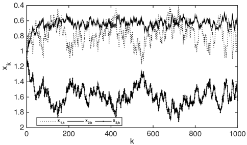
Figure 1: One realization of identification data from the compartmental model. The state components are shown evolving with time.

We investigate a 1000-run Monte Carlo simulation testing identification data with different noise realizations for $\sigma_{w}$ $=$ $1.0$ and $\sigma_{v}$ $=$ $0.1$. The LS given by (26) for the state-space system, for which (6)-(20) are defined, is used to yield estimates for the matrix $A$ as discussed in Section 2. Likewise, as indicated by Proposition 4.3, CLS was also employed.

Fig. 2 shows the results regarding the Monte Carlo validation of the obtained models (mean values with two standard-devation confidence interval). In order to quantify the fit between the simulation of the system and the identified models, we use the root-mean-square error for each $i$th state component, $i=1,\ldots,n$,

$$\textrm{RMSE}^{m_{r}}_{n}\triangleq\sqrt{\frac{\sum^{N}_{k=1}(x_{i,k}-\hat{x}_{i,k})^{2}}{N}},$$ (71)

where $N$ is the length of the measured data and $m_{r}=1,\ldots,M$, where $M$ is the number of realizations. Table 5.1 shows the mean $\overline{\textrm{RMSE}}_{n}$ and standard deviation $\sigma_{\rm{RMSE}_{n}}$ of the RMSE for each state. Note that the performance of the model obtained with CLS is better than the model estimated by LS. That is, the auxiliary information about mass conservation was useful.

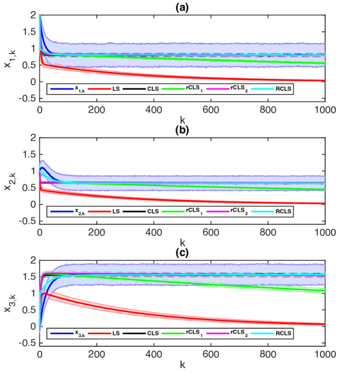
Figure 2: Comparison of $1000$-run Monte Carlo simulations for the validation of state-space models identified using LS (red line), CLS (black line) and RCLS (cyan line). To address the case of uncertain prior information, we estimate models using rCLS, for which we test two values of the tuning parameter: $\mu_{1}=5\times 10^{3}$ (green line) and $\mu_{2}=5\times 10^{4}$ (magenta line). The mean of true values of the states are shown in a blue continuous line. In all cases, the mean values of the validation data are shown within the confidence interval of two standard deviations given by the respective light shaded areas.

In addition, we consider the case where the auxiliary information is uncertain. Suppose that the uncertain state equality constraint is assumed to be given by (3) with

$$S=[1.4~{}~{}0.9~{}~{}1.2],~{}~{}s=3.5.$$ (72)

The rCLS given by (30) is used to estimate the state-space model with the uncertain auxiliary information (72). As in Arablouei  Dogançay (2015), we tuned the parameter $\mu$ in order to obtain models with good prediction performance. The results are shown in Fig. 2 and Table 5.1 for $\mu_{1}=5\times 10^{3}$ ($\rm{rCLS}_{1}$) and $\mu_{2}=5\times 10^{4}$ ($\rm{rCLS}_{2}$). Note that the results yielded by ($\rm{rCLS}_{1}$) are better than those from LS. Moreover, results from $\rm{rCLS}_{2}$ almost coincide to those from CLS. Then, the appropriate use of uncertain prior information may improve the quality of the estimated model, as discussed in Teixeira  Aguirre (2011).

We also test the recursive solution to this problem as indicated by Corollary 4.4. RLS is properly initialized as in (34)-(35), with $\theta_{0}$ $=$ $0_{9\times 1}$ and $P_{0}$ $=$ $10^{3}I_{9\times 9}$, yielding RCLS and is compared with the batch LS and CLS estimates in Fig. 2 and Table 5.1. Note that, when compared to LS, the use of auxiliary information (70) in the initialization of RCLS improves the performance of the estimated model.

The mean and the standard deviation of the RMSE for 1000-run Monte Carlo simulations of each state sequence. Method $\hfil\!\overline{\textrm{RMSE}}_{1}\!\!\pm\!\sigma_{\rm{RMSE}_{1}}$ $\hfil\!\overline{\textrm{RMSE}}_{2}\!\!\pm\!\sigma_{\rm{RMSE}_{2}}$ $\hfil\!\overline{\textrm{RMSE}}_{3}\!\!\pm\!\sigma_{\rm{RMSE}_{3}}$ LS 0.660 $\pm$ 0.029 0.527 $\pm$ 0.013 1.248 $\pm$ 0.038 CLS 0.191 $\pm$ 0.012 0.134 $\pm$ 0.003 0.211 $\pm$ 0.014 $\rm{rCLS_{1}}$ 0.232 $\pm$ 0.020 0.169 $\pm$ 0.007 0.356 $\pm$ 0.031 $\rm{rCLS_{2}}$ 0.189 $\pm$ 0.012 0.133 $\pm$ 0.003 0.219 $\pm$ 0.016 RCLS 0.202 $\pm$ 0.013 0.116 $\pm$ 0.003 0.196 $\pm$ 0.015

5.2 Compartmental system: time-varying case

We now consider a time-varying compartmental system. As in a reconfigurable system, we consider the case in which the linear dynamics switches among three different modes. For instance, this may be the case for a multi-tank system with reconfigurable valves. The first mode is simulated with $A_{1}$ as in (69). The second and third modes are described by the matrices

$$A_{2}=\left[\begin{array}[]{ccc}0.84&0.028&0.019\\ 0.138&0.85&0.001\\ 0.022&0.122&0.98\end{array}\right],$$

$$A_{3}=\left[\begin{array}[]{ccc}0.80&0.018&0.119\\ 0.178&0.76&0.201\\ 0.022&0.222&0.68\end{array}\right].$$

The matrices $B$ and $C$ are defined as in (69) for all modes.

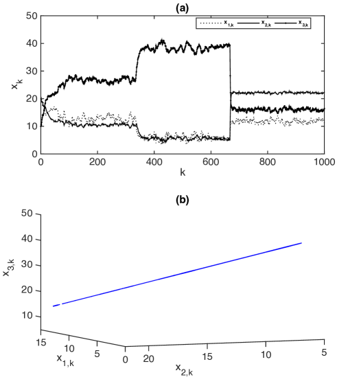
Figure 3: One realization of the identification data for the time-varying compartmental model. In (a), the state components are shown evolving with time and, in (b), in state space. Note that, regardless of the mode, for all $k$ $\geq$ $0$, $x_{k}$ $\in$ $\mathbb{R}$ lies on the plane $x_{1,k}$ $+$ $x_{2,k}$ $+$ $x_{3,k}$ $=$ $50$.

A typical realization of the simulated identification data is shown in Fig. 3 for $\sigma_{w}$ $=$ $10$ and $\sigma_{v}$ $=$ $1$ and $x_{0}$ $=$ $[20~{}~{}20~{}~{}10]^{T}$. The mass conservation is verified for all operating points and the assumedly known parameters of (3) are given by

$$S=[1~{}~{}1~{}~{}1],~{}~{}s=50.$$ (73)

Note that the conditions of Lemmas 4.1 and 4.2 are verified for all modes. A new initial condition is set as $x_{0}$ $=$ $[15~{}~{}10~{}~{}25]^{T}$ to simulate the validation data.

We generate $1000$ Monte Carlo simulations with different noise realizations for $\sigma_{w}$ $=$ $10$ and $\sigma_{v}$ $=$ $1$ in order to obtain the identification data. For each running simulation we employ both RWLS given by (38)-(40) and RWCLS given by (38)-(42) to estimate the time-varying model. These recursive estimators are randomly initialized with an arbitrary initial condition ${\rm vec}(\Theta_{0})\in\mathbb{R}^{{9\times 1}}$ given by a normal distribution with $\sigma_{\Theta}=1$ and $P_{0}=10^{4}I_{9\times 9}$. Recall that in Alenany  Shang (2013) part of the identification data is used to estimate de initial conditions by means of the batch algorithm (25); see Remark 2. Here, we use the result given by (34)-(35) to more conveniently proceed the identification procedure using the RWCLS. The forgetting factor $\lambda$ is set to $0.95$.

The Monte Carlo validation results for RWLS and RWCLS are shown in Fig. 4. We would like to draw attention to the variance of the estimated models. For the three different modes, we verify that the performance of the model obtained with RWCLS is better than the model estimated by RWLS. That is, the prior information about mass conservation improved the quality of the estimated model.

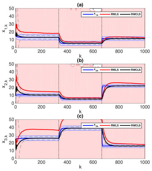
Figure 4: Comparison of $1000$-run Monte Carlo simulations for the validation of state-space models identified using RWLS (red line) and RWCLS (black line), where the RWCLS is initialized in according to (34)-(35) and the constraint is enforced with (41)-(42). The mean of true values of the states are shown in a blue continuous line. In all cases, the mean values of the validation data are shown within the confidence interval of two standard deviations given by the respective light shaded areas. Observe that the confidence interval of RWLS are partially presented. Dotted vertical black lines show when the operating points are switched.

5.3 Practical application: forest ecosystem

Consider the compartmental model of nitrogen flow in a tropical forest studied in Walter  Contreras (1999) and summarized in Figure 5, where $k_{ij}$ accounts for the flow rates between compartments, associated with the mass leaving the $i$th compartment and arriving at the $j$th compartment. Note that each compartment allows interaction from its neighbour compartments in both directions and that the parameters are given for a continuous-time model. Choosing the sampling-period as $T_{s}=0.1$ years, the discrete-time matrices are given by

$$A\!\! \!\!=\!\! \!\!\left[\begin{array}[]{ccccc}0.9003&0&0.0005&0&0.0093\\ 0.0935&0.8807&0&0&0.0005\\ 0.0054&0.0978&0.6697&0&0\\ 0.0005&0.0154&0.2372&0.9995&0\\ 0.0002&0.0060&0.0927&0.005&0.9902\end{array}\right],$$ (78)

$$B\!\! \!\!=\!\! \!\!\left[\begin{array}[]{ccccc}0.5505\!&\!0.0282\!&\!-0.2625\!&\!-0.3003\!&\!-0.0159\end{array}\right]^{T},$$

$$C\!\! \!\!=\!\! \!\!I_{5\times 5},$$ (80)

with state vector $x_{k}$ $\in$ $\mathbb{R}^{5}$ composed by the amount of nitrogen in each compartment, initial condition $x_{0}\!\!=\!\![\!-\!3.5~{}\!-\!2.52~{}~{}0~{}~{}520~{}~{}26.5]^{T}\!\!+\!\!\mathcal{K}[3.82~{}~{}316~{}~{}1~{}~{}576~{}~{}41\!]^{T}$, where $\mathcal{K}$ depends on the total amount of nitrogen in the system in the beginning and is set as $\mathcal{K}=1.5$, the process noise and observation noise covariance matrices $\tilde{Q}$ $=$ $\sigma_{w}^{2}GG^{T}$, where $G=\left[\begin{array}[]{cccc}0.1220&0.1634&0.0249&-0.0383\\ -0.0420&-0.0048&-0.1430&0.0235\\ 0.1640&-0.0317&-0.0057&0.0571\\ -0.1871&-0.0877&0.1697&-0.0098\\ -0.0569&-0.0392&-0.0459&-0.0325\end{array}\right]$, and $R_{k}=\sigma_{v}^{2}I_{4\times 4}$. The conditions of Lemmas 4.1 and 4.2 hold for (78) such that the trajectory of $x_{k}$ $\in$ $\mathbb{R}^{5}$ lies on the plane (3), whose parameters are assumed to be known and are given by

$$S=[1~{}~{}1~{}~{}1~{}~{}1~{}~{}1],~{}~{}s=1.9472\times 10^{3}.$$ (81)

that is, mass conservation is verified.

We investigate a 1000-run Monte Carlo simulation testing identification data with $u_{k}=1+\sigma_{u}w_{k}^{u}$ and different noise realizations for $\sigma_{u}$ $=$ $0.1$, $\sigma_{w}$ $=$ $1.0$ and $\sigma_{v}$ $=$ $1.0$ (not shown for brevity), where $w^{u}$ is a zero mean white noise to ensure the persistence of excitation of the input. For each running simulation we employ both LS given by (26) and CLS given by Proposition 4.3. The validation data is simulated with different initial condition $x_{0}\!\!=\!\![72.2~{}~{}381.5~{}~{}101.5~{}~{}1264.0~{}~{}128.0]^{T}$. Figure 6 shows the results regarding the RMSE of the Monte Carlo validation of the obtained models. For all the states the use of auxiliary information in the CLS improves the performance of the estimated models. Specifically, the CLS estimation of the $4$th and $5$th state components always outperform the LS estimation. For in the CLS estimator, $\overline{\textrm{RMSE}}_{4}$ is around $15$ times smaller than the same index for LS. For the $5$th state, CLS improves $\overline{\textrm{RMSE}}_{5}$ by a factor of 3.

Figure 5: Schematic compartmental model of nitrogen flow in a tropical forest. The inputs and outputs are assumed to be constant in the model. Adapted from Walter  Contreras (1999).

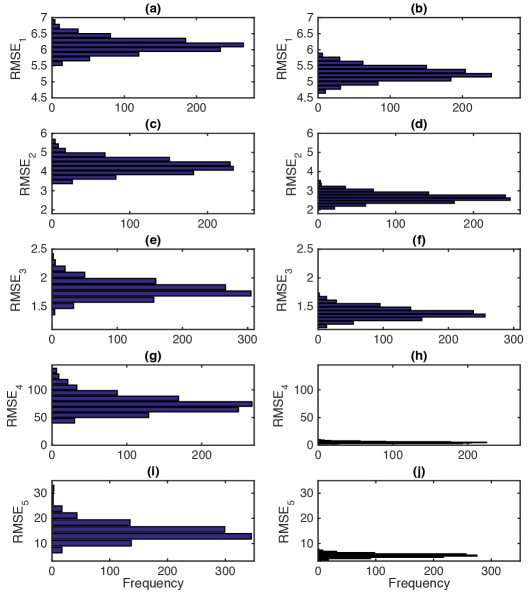
Figure 6: Histogram of the RMSE between the validation data and LS (left) and CLS (right) estimation for all the $1000$-run Monte Carlo simulations.

6 Concluding Remarks

We address the problem of modeling state-space dynamic systems for which the state vector satisfies an exactly known or an uncertain equality constraint (prior information). We assume that all state components are measured such that least-square methods can be used to estimate the state-space matrices. Both batch and recursive algorithms are considered. By means of the latter, the time-varying case is also addressed.

First, we show how to map the known equality constraint on the state vector on an equality constraint on the parameter matrix to be estimated by the least-square based method. Then, we show how to rewrite the corresponding least squares problem into a vectorized form such that existing equality-constrained least squares methods may be used.

In addition to obtaining state-space matrices that yield an equality-constrained model on the state vector, we observe that the usage of both exactly known and uncertain prior information improves the prediction quality of the model compared to the case in which the equality constraint is not enforced. Such results are consistent with those from Teixeira  Aguirre (2011). The algorithms here investigated are also of interest for gray-box subspace identification methods that employ least squares as an internal step; see Trnka  Havlena (2009); Alenany . (2011); Privara . (2012); Alenany  Shang (2013).

Appendix A

Next, we present the proof of Proposition 3.1.

Proof.

Given that (27) is a projector onto the null space of $D$, initialize the RLS equations given by (31)-(33) with the initial values (34)-(35) such that

$$D\hat{\theta}_{\textrm{CLS},0} = d,$$ (82)

$$DP_{\textrm{CLS},0} = 0.$$ (83)

For $k=1$, multiplying (31)-(33) by $D$ we have

$$DK_{1} = \frac{DP_{\textrm{CLS},0}\psi_{0}}{\psi^{T}_{0}P_{\textrm{CLS},0}\psi_{0}+1}=0,$$ (84)

$$D\hat{\theta}_{\textrm{CLS},1} = D{\theta}_{\textrm{CLS},0}+DK_{1}\left(z_{1}-\psi^{T}_{0}{\theta}_{\textrm{CLS},0}\right),$$ (85)

$$= d,$$

$$DP_{\textrm{CLS},1} = D\left(I_{n_{p}}-K_{1}\psi_{0}^{T}\right)P_{\textrm{CLS},0},$$ (86)

$$= DP_{\textrm{CLS},0}-DK_{1}\psi_{0}^{T}P_{\textrm{CLS},0}=0.$$

By symmetry, from (84)-(85), we verify that $DK_{2}=0$, $D\hat{\theta}_{\textrm{CLS},2}=d$ and $DP_{\textrm{CLS},2}=0$.

Likewise, at time $k+1$, we have $DK_{k+1}=0$, $D\hat{\theta}_{\textrm{CLS},k+1}=d$ and $DP_{\textrm{CLS},k+1}=0$.

Thus, by induction, we have $DK_{k}=0$, $D\hat{\theta}_{\textrm{CLS},k}=d$ and $DP_{\textrm{CLS},k}=0$, $\forall$ $k$, completing the proof. ∎

Appendix B

In the following, we show that the classical LS estimator is biased for the estimation of the matrices of the state-space model (1)-(2).

Proof.

Replace $y_{k}$ in (4), write this result as the linear regression model (21) and apply the vectorization operador (68), then we obtain

$$\textrm{vec}(y_{k+1})=\Psi_{k}^{T}\theta+\textrm{vec}(e_{k+1}).$$

where

$$\Psi_{k}^{T}\! \!\!\!=\!\!\! \!\left[\!\!\!\begin{array}[]{cc}\left\{\!\left[\!\begin{array}[]{cc}y_{k-1}^{T}\!\!\otimes\!\!I_{n}&u^{T}_{k-1}\!\!\otimes\!\!I_{n}\end{array}\!\!\right]\theta+\textrm{vec}(e_{k})\!\right\}\!\!\otimes\!\!I_{n}&u^{T}_{k}\!\!\otimes\!\!I_{n}\end{array}\!\!\right],$$ (89)

$$e_{k+1}\! \!\!\!=\!\!\! \!v_{k+1}-A\underline{v_{k}}+Gw_{k},$$

$$e_{k}\! \!\!\!=\!\!\! \!\underline{v_{k}}-Av_{k-1}+Gw_{k-1}.$$

The terms $v_{k}$ underlined are identical. So, the regressor $y_{k}$ between the braces is correlated with $e_{k+1}$. In this case, the LS estimator is biased. ∎

References

- Aguirre \BOthers. (\APACyear2007) \APACinsertmetastar2007_Aguirre_Alves_Correa{APACrefauthors}Aguirre, L\BPBIA., Alves, G\BPBIB.\BCBL \BBA Corrêa, M\BPBIV. \APACrefYearMonthDay2007. \BBOQ\APACrefatitleSteady-state Performance Constraints for Dynamical Models Based on RBF Networks Steady-state Performance Constraints for Dynamical Models Based on RBF Networks.\BBCQ \APACjournalVolNumPagesEngineering Applications of Artificial Intelligence207924-935. \PrintBackRefs\CurrentBib
- Alenany \BBA Shang (\APACyear2013) \APACinsertmetastarAlenany2013{APACrefauthors}Alenany, A.\BCBT \BBA Shang, H. \APACrefYearMonthDay2013. \BBOQ\APACrefatitleRecursive subspace identification with prior information using the constrained least squares approach Recursive subspace identification with prior information using the constrained least squares approach.\BBCQ \APACjournalVolNumPagesComputers & Chemical Engineering54174 - 180. \PrintBackRefs\CurrentBib
- Alenany \BOthers. (\APACyear2011) \APACinsertmetastarAlenany2011{APACrefauthors}Alenany, A., Shang, H., Soliman, M.\BCBL \BBA Ziedan, I. \APACrefYearMonthDay2011Sept. \BBOQ\APACrefatitleBrief paper - Improved subspace identification with prior information using constrained least squares Brief paper - Improved subspace identification with prior information using constrained least squares.\BBCQ \APACjournalVolNumPagesIET Control Theory Applications5131568-1576. {APACrefDOI} 10.1049/iet-cta.2010.0585 \PrintBackRefs\CurrentBib
- Arablouei \BBA Dogançay (\APACyear2015) \APACinsertmetastararablouei2015{APACrefauthors}Arablouei, R.\BCBT \BBA Dogançay, K. \APACrefYearMonthDay2015. \BBOQ\APACrefatitlePerformance analysis of linear-equality-constrained least-squares estimation Performance analysis of linear-equality-constrained least-squares estimation.\BBCQ \APACjournalVolNumPagesIEEE Transactions on Signal Processing63143762–3769. \PrintBackRefs\CurrentBib
- Babacan \BOthers. (\APACyear2008) \APACinsertmetastarBabacan2008{APACrefauthors}Babacan, E\BPBIK., Ozbek, L.\BCBL \BBA Efe, M. \APACrefYearMonthDay2008Dec. \BBOQ\APACrefatitleStability of the Extended Kalman Filter When the States are Constrained Stability of the Extended Kalman Filter When the States are Constrained.\BBCQ \APACjournalVolNumPagesIEEE Transactions on Automatic Control53112707-2711. {APACrefDOI} 10.1109/TAC.2008.2008333 \PrintBackRefs\CurrentBib
- Bernstein (\APACyear2005) \APACinsertmetastarBernstein2005{APACrefauthors}Bernstein, D\BPBIS. \APACrefYear2005. \APACrefbtitleMatrix mathematics: theory, facts, and formulas with application to linear systems theory Matrix mathematics: theory, facts, and formulas with application to linear systems theory (\PrintOrdinal1 \BEd). \APACaddressPublisherPrinceton, New Jersey, USAPrinceton University Press. \PrintBackRefs\CurrentBib
- Bernstein \BBA Hyland (\APACyear1993) \APACinsertmetastar1993_Hyland_Bernstein{APACrefauthors}Bernstein, D\BPBIS.\BCBT \BBA Hyland, D\BPBIC. \APACrefYearMonthDay1993. \BBOQ\APACrefatitleCompartmental Modeling and Second-Moment Analysis of State Space Systems Compartmental Modeling and Second-Moment Analysis of State Space Systems.\BBCQ \APACjournalVolNumPagesSIAM Journal on Matrix Analysis and Applications143880-901. \PrintBackRefs\CurrentBib
- Björck (\APACyear1996) \APACinsertmetastarBjork1996{APACrefauthors}Björck, A. \APACrefYear1996. \APACrefbtitleNumerical Methods for Least Squares Problems Numerical Methods for Least Squares Problems (\PrintOrdinal1 \BEd). \APACaddressPublisherLinköping, SwedenLinköping University. \PrintBackRefs\CurrentBib
- Crassidis \BBA Markley (\APACyear2003) \APACinsertmetastar2003_Crassidis_Markley{APACrefauthors}Crassidis, J\BPBIL.\BCBT \BBA Markley, F\BPBIL. \APACrefYearMonthDay2003. \BBOQ\APACrefatitleUnscented Filtering for Spacecraft Attitude Estimation Unscented Filtering for Spacecraft Attitude Estimation.\BBCQ \APACjournalVolNumPagesAIAA Journal of Guidance, Control, and Dynamics264536-542. \PrintBackRefs\CurrentBib
- Draper \BBA Smith (\APACyear1998) \APACinsertmetastardraper1998{APACrefauthors}Draper, N\BPBIR.\BCBT \BBA Smith, H. \APACrefYear1998. \APACrefbtitleApplied Regression Analysis Applied Regression Analysis. \APACaddressPublisherNew York, USAJohn Wiley & Sons. \PrintBackRefs\CurrentBib
- Duan \BBA Li (\APACyear2015) \APACinsertmetastarDuan_and_Li2015{APACrefauthors}Duan, Z.\BCBT \BBA Li, X\BPBIR. \APACrefYearMonthDay2015Oct. \BBOQ\APACrefatitleAnalysis, design, and estimation of linear equality-constrained dynamic systems Analysis, design, and estimation of linear equality-constrained dynamic systems.\BBCQ \APACjournalVolNumPagesIEEE Transactions on Aerospace and Electronic Systems5142732-2746. {APACrefDOI} 10.1109/TAES.2015.140441 \PrintBackRefs\CurrentBib
- Goodwin \BOthers. (\APACyear2005) \APACinsertmetastar2005_Goodwin_Seron_Dona{APACrefauthors}Goodwin, G\BPBIC., Seron, M\BPBIM.\BCBL \BBA de Doná, J\BPBIA. \APACrefYear2005. \APACrefbtitleConstrained Control and Estimation: An Optimization Approach Constrained Control and Estimation: An Optimization Approach. \APACaddressPublisherLondonSpringer. \PrintBackRefs\CurrentBib
- Hölzel \BBA Bernstein (\APACyear2014) \APACinsertmetastarHolzel2014{APACrefauthors}Hölzel, M\BPBIS.\BCBT \BBA Bernstein, D\BPBIS. \APACrefYearMonthDay2014. \BBOQ\APACrefatitleA matrix nullspace approach for solving equality-constrained multivariable polynomial least-squares problems A matrix nullspace approach for solving equality-constrained multivariable polynomial least-squares problems.\BBCQ \APACjournalVolNumPagesAutomatica50123030 - 3037. {APACrefDOI} http://dx.doi.org/10.1016/j.automatica.2014.10.039 \PrintBackRefs\CurrentBib
- Lee \BOthers. (\APACyear2017) \APACinsertmetastarLee2017{APACrefauthors}Lee, K\BPBIF., Dosta, M., McGuire, A\BPBID., Mosbach, S., Wagner, W., Heinrich, S.\BCBL \BBA Kraft, M. \APACrefYearMonthDay2017. \BBOQ\APACrefatitleDevelopment of a multi-compartment population balance model for high-shear wet granulation with discrete element method Development of a multi-compartment population balance model for high-shear wet granulation with discrete element method.\BBCQ \APACjournalVolNumPagesComputers & Chemical Engineering99171 - 184. {APACrefDOI} https://doi.org/10.1016/j.compchemeng.2017.01.022 \PrintBackRefs\CurrentBib
- Li (\APACyear2016) \APACinsertmetastar2016_Li{APACrefauthors}Li, X\BPBIR. \APACrefYearMonthDay2016July. \BBOQ\APACrefatitleCompatibility and modeling of constrained dynamic systems Compatibility and modeling of constrained dynamic systems.\BBCQ \BIn \APACrefbtitle2016 19th International Conference on Information Fusion (FUSION) 2016 19th international conference on information fusion (fusion) (\BPG 240-247). \PrintBackRefs\CurrentBib
- Ljung (\APACyear1987) \APACinsertmetastarLjung1987{APACrefauthors}Ljung, L. \APACrefYear1987. \APACrefbtitleSystem Identification: Theory for the User System Identification: Theory for the User. \APACaddressPublisherLondonPrentice-Hall. \PrintBackRefs\CurrentBib
- Massicotte \BOthers. (\APACyear1995) \APACinsertmetastar1995_Massicotte_Morawski_Barwicz{APACrefauthors}Massicotte, D., Morawski, R\BPBIZ.\BCBL \BBA Barwicz, A. \APACrefYearMonthDay1995Feb. \BBOQ\APACrefatitleIncorporation of a Positivity Constraint into a Kalman-Filter-Based Algorithm for Correction of Spectrometric Data Incorporation of a Positivity Constraint into a Kalman-Filter-Based Algorithm for Correction of Spectrometric Data.\BBCQ \APACjournalVolNumPagesIEEE Transactions on Instrumentation and Measurement4412-7. {APACrefDOI} 10.1109/19.368111 \PrintBackRefs\CurrentBib
- Mohler (\APACyear1974) \APACinsertmetastar1974_Mohler{APACrefauthors}Mohler, R. \APACrefYearMonthDay1974Dec. \BBOQ\APACrefatitleBiological modeling with variable compartmental structure Biological modeling with variable compartmental structure.\BBCQ \APACjournalVolNumPagesIEEE Transactions on Automatic Control196922-926. {APACrefDOI} 10.1109/TAC.1974.1100739 \PrintBackRefs\CurrentBib
- Privara \BOthers. (\APACyear2012) \APACinsertmetastarprivara2012{APACrefauthors}Privara, S., Cigler, J., Vaná, Z.\BCBL \BBA Ferkl, L. \APACrefYearMonthDay2012. \BBOQ\APACrefatitleIncorporation of system steady state properties into subspace identification algorithm Incorporation of system steady state properties into subspace identification algorithm.\BBCQ \APACjournalVolNumPagesInternational Journal of Modelling, Identification and Control162159–167. {APACrefDOI} 10.1504/IJMIC.2012.047123 \PrintBackRefs\CurrentBib
- Rengaswamy \BOthers. (\APACyear2013) \APACinsertmetastarRengaswamy2013{APACrefauthors}Rengaswamy, R., Narasimhan, S.\BCBL \BBA Kuppuraj, V. \APACrefYearMonthDay2013Aug. \BBOQ\APACrefatitleReceding-Horizon Nonlinear Kalman (RNK) Filter for State Estimation Receding-Horizon Nonlinear Kalman (RNK) Filter for State Estimation.\BBCQ \APACjournalVolNumPagesIEEE Transactions on Automatic Control5882054-2059. {APACrefDOI} 10.1109/TAC.2013.2253271 \PrintBackRefs\CurrentBib
- Simon (\APACyear2010) \APACinsertmetastar2010_Simon{APACrefauthors}Simon, D. \APACrefYearMonthDay2010August. \BBOQ\APACrefatitleKalman filtering with state constraints: a survey of linear and nonlinear systems Kalman filtering with state constraints: a survey of linear and nonlinear systems.\BBCQ \APACjournalVolNumPagesIET Control Theory and Applications481303–1318. {APACrefDOI} 10.1049/iet-cta.2009.0032 \PrintBackRefs\CurrentBib
- Teixeira \BBA Aguirre (\APACyear2011) \APACinsertmetastar2011_Teixeira_Aguirre{APACrefauthors}Teixeira, B\BPBIO\BPBIS.\BCBT \BBA Aguirre, L\BPBIA. \APACrefYearMonthDay2011. \BBOQ\APACrefatitleUsing uncertain prior knowledge to improve identified nonlinear dynamic models Using uncertain prior knowledge to improve identified nonlinear dynamic models.\BBCQ \APACjournalVolNumPagesJournal of Process Control21182–91. \PrintBackRefs\CurrentBib
- Teixeira \BOthers. (\APACyear2008) \APACinsertmetastarTeixeira2008{APACrefauthors}Teixeira, B\BPBIO\BPBIS., Chandrasekar, J., Palanthandalam-Madapusi, H\BPBIJ., Tôrres, L., Aguirre, L\BPBIA.\BCBL \BBA Bernstein, D\BPBIS. \APACrefYearMonthDay2008\APACmonth09. \BBOQ\APACrefatitleGain-Constrained Kalman Filtering for Linear and Nonlinear Systems Gain-Constrained Kalman Filtering for Linear and Nonlinear Systems.\BBCQ \APACjournalVolNumPagesIEEE Transactions on Signal Processing5694113–4123. {APACrefDOI} 10.1109/TSP.2008.926101 \PrintBackRefs\CurrentBib
- Teixeira \BOthers. (\APACyear2009) \APACinsertmetastarTeixeira2009{APACrefauthors}Teixeira, B\BPBIO\BPBIS., Chandrasekar, J., Tôrres, L\BPBIA\BPBIB., Aguirre, L\BPBIA.\BCBL \BBA Bernstein, D\BPBIS. \APACrefYearMonthDay2009. \BBOQ\APACrefatitleState estimation for linear and non-linear equality-constrained systems State estimation for linear and non-linear equality-constrained systems.\BBCQ \APACjournalVolNumPagesInternational Journal of Control825918–936. {APACrefDOI} 10.1080/00207170802370033 \PrintBackRefs\CurrentBib
- Trnka \BBA Havlena (\APACyear2009) \APACinsertmetastarTrnka2009{APACrefauthors}Trnka, P.\BCBT \BBA Havlena, V. \APACrefYearMonthDay2009. \BBOQ\APACrefatitleSubspace like identification incorporating prior information Subspace like identification incorporating prior information.\BBCQ \APACjournalVolNumPagesAutomatica4541086 - 1091. {APACrefDOI} http://dx.doi.org/10.1016/j.automatica.2008.12.005 \PrintBackRefs\CurrentBib
- Vincent \BBA Chaumette (\APACyear2018) \APACinsertmetastarVINCENT_2018{APACrefauthors}Vincent, F.\BCBT \BBA Chaumette, E. \APACrefYearMonthDay2018. \BBOQ\APACrefatitleRecursive linearly constrained minimum variance estimator in linear models with non-stationary constraints Recursive linearly constrained minimum variance estimator in linear models with non-stationary constraints.\BBCQ \APACjournalVolNumPagesSignal Processing149229 - 235. {APACrefDOI} https://doi.org/10.1016/j.sigpro.2018.03.016 \PrintBackRefs\CurrentBib
- Walter \BBA Contreras (\APACyear1999) \APACinsertmetastarWalter1999{APACrefauthors}Walter, G\BPBIG.\BCBT \BBA Contreras, M. \APACrefYear1999. \APACrefbtitleCompartmental Modeling with Networks Compartmental Modeling with Networks. \APACaddressPublisherBirkhäuser BostonBirkhäuser Basel. \PrintBackRefs\CurrentBib
- Wang \BOthers. (\APACyear2018) \APACinsertmetastar2018_Youqing{APACrefauthors}Wang, Y., Zhang, L.\BCBL \BBA Zhao, Y. \APACrefYearMonthDay2018. \BBOQ\APACrefatitleImproved closed-loop subspace identification with prior information Improved closed-loop subspace identification with prior information.\BBCQ \APACjournalVolNumPagesInternational Journal of Systems Science4991821-1835. {APACrefDOI} 10.1080/00207721.2018.1460409 \PrintBackRefs\CurrentBib
- Xu \BOthers. (\APACyear2013) \APACinsertmetastarXu2013{APACrefauthors}Xu, L., Li, X\BPBIR., Duan, Z.\BCBL \BBA Lan, J. \APACrefYearMonthDay2013. \BBOQ\APACrefatitleModeling and State Estimation for Dynamic Systems With Linear Equality Constraints Modeling and State Estimation for Dynamic Systems With Linear Equality Constraints.\BBCQ \APACjournalVolNumPagesIEEE Transactions on Signal Processing61112927-2939. {APACrefDOI} 10.1109/TSP.2013.2255045 \PrintBackRefs\CurrentBib
- Xu \BOthers. (\APACyear2017) \APACinsertmetastarXu_2017{APACrefauthors}Xu, L., Li, X\BPBIR., Liang, Y.\BCBL \BBA Duan, Z. \APACrefYearMonthDay20175. \BBOQ\APACrefatitleConstrained Dynamic Systems: Generalized Modeling and State Estimation Constrained Dynamic Systems: Generalized Modeling and State Estimation.\BBCQ \APACjournalVolNumPagesIEEE Transactions on Aerospace and Electronic SystemsPP991-14. {APACrefDOI} 10.1109/TAES.2017.2705518 \PrintBackRefs\CurrentBib
- Zhou \BOthers. (\APACyear2001) \APACinsertmetastarZhou_et_al_2001{APACrefauthors}Zhou, J., Zhu, Y., Li, X\BPBIR.\BCBL \BBA You, Z. \APACrefYearMonthDay2001. \BBOQ\APACrefatitleExactly Initialized Recursive Least Squares Exactly Initialized Recursive Least Squares.\BBCQ \BIn \APACrefbtitleProceedings of the 40th IEEE Conference on Decision and Control Proceedings of the 40th ieee conference on decision and control (\BPG 3318-3323). \APACaddressPublisherOrlando, Florida, USA. \PrintBackRefs\CurrentBib
- Zhu \BBA Li (\APACyear2007) \APACinsertmetastarZhuLi2007{APACrefauthors}Zhu, Y.\BCBT \BBA Li, X\BPBIR. \APACrefYearMonthDay2007. \BBOQ\APACrefatitleRecursive Least Squares with Linear Constraints Recursive Least Squares with Linear Constraints.\BBCQ \APACjournalVolNumPagesCommunications in Information and Systems73287–312. \PrintBackRefs\CurrentBib