Joint Manifold Diffusion for Combining Predictions on Decoupled Observations

Abstract

We present a new predictor combination algorithm that improves a given task predictor based on potentially relevant reference predictors. Existing approaches are limited in that, to discover the underlying task dependence, they either require known parametric forms of all predictors or access to a single fixed dataset on which all predictors are jointly evaluated. To overcome these limitations, we design a new non-parametric task dependence estimation procedure that automatically aligns evaluations of heterogeneous predictors across disjoint feature sets. Our algorithm is instantiated as a robust manifold diffusion process that jointly refines the estimated predictor alignments and the corresponding task dependence. We apply this algorithm to the relative attributes ranking problem and demonstrate that it not only broadens the application range of predictor combination approaches but also outperforms existing methods even when applied to classical predictor combination settings.

1 Introduction

When the performance of an estimated predictor is not adequate for the task at hand, e.g. due to limited training examples, we might benefit from the knowledge gained from related tasks. Multi-task learning (MTL) [1, 12, 16, 19] explores this possibility by solving multiple problems simultaneously, and so capturing and benefiting from the potential task dependence. The success of MTL in many visual learning problems has demonstrated such task dependence [1, 12, 23, 19, 10]. In most existing MTL algorithms, task dependence is modeled through the latent structures on the parameter spaces of the corresponding task predictors. For instance, Evgeniou and Pontil’s algorithm [6] penalizes pair-wise parameter deviations of task predictors. Since it is unlikely that all tasks exhibit known task dependence structure, MTL algorithms attempt to automatically discover the underlying dependence and identify outliers, by e.g. enforcing sparsity and/or introducing low-rank constraints on the aggregated task parameter matrices [1, 8] or by explicitly performing clustering of tasks [25, 18].

A major limitation of these traditional MTL approaches is that they require all task predictors to share the same predictive model or even the same parameter space, making them difficult to apply to heterogeneous predictors, e.g. combining deep neural networks and support vector machines. However, the best predictor forms often depend on the individual tasks of interest. Further, existing MTL approaches are designed to train multiple predictors simultaneously, and so they cannot be directly applied to train a new task predictor given previously-trained reference predictors, e.g. combining pre-trained or pre-compiled predictor libraries without access to the corresponding task training data.

Recently, Kim et al. [10] proposed a non-parametric predictor combination approach where the predictor evaluations made at sampled data points are improved by combining them with reference predictions at test time without requiring simultaneous training. This enables us to combine predictors with different or even unknown parametric forms. However, the application scope of this approach is limited in its own way, as it requires a large set of data points on which all predictors are jointly evaluated. In practical applications, different predictions can be constructed based on the respective feature representations tailored for specific tasks of interest, and often these features are available by themselves as separate databases without having explicit references to the corresponding source data (e.g. images).

In this paper, we propose a new algorithm to avoid the limitations of previous predictor combination approaches, thereby broadening the application spectrum of the non-parametric predictor combination approach [10]. Building on their test-time combination approach, our algorithm improves a task predictor based on a set of reference predictors. However, unlike their approach, we do not require that all predictors are available for evaluation on a single fixed set. Our algorithm takes as input decoupled predictor evaluations and automatically aligns these predictions to discover the underlying task dependence. As the initial estimates of the alignments and the corresponding task dependence might be noisy, we denoise them jointly via a manifold diffusion process. The new algorithm combines the benefits of classical parametric MTL approaches and recent test-time combination algorithms, and facilitates combination applications where multiple heterogeneous predictors are constructed from disjoint feature sets. We apply our algorithm to the relative attributes ranking problem, and extend the application over previous approaches. Furthermore, evaluated on seven challenging datasets, our approach demonstrates that even when applied in the restricted settings of traditional approaches, it significantly improves both accuracy and time efficiency.

Relative attributes ranking: Relative attributes ranking [17, 11] refers to the problem of inferring a linear ordering of database images based on the strengths of attribute present in each entry. This problem differs from binary attribute classification where the goal is to predict the presence or absence of an attribute. Instead, relative attributes ranking focuses on attributes where such clear binary classifications cannot be obtained, e.g. a shoe $A$ can be ‘more formal’ than $B$ but it could still appear ‘less formal’ than $C$. This problem is also different from classical data-retrieval type ranking applications where the goal is to identify database entries that match a given query.

This goal can be achieved by learning a rank function $f$ based on user-provided rank labels: Given a set of data points $X=\{\mathbf{x}_{1},\ldots,\mathbf{x}_{n}\}\subset\mathcal{X}$, rank learning aims to construct a function $f:\mathcal{X}\to\mathbb{R}$ that agrees with the observed pair-wise rank labels $R=\{(i(1),j(1)),\ldots,(i(l),j(l))\}\subset X\times X$ where $(i,j)\in R$ implies that the rank of $\mathbf{x}_{i}$ is higher than $\mathbf{x}_{j}$: $f(\mathbf{x}_{i})>f(\mathbf{x}_{j})$. For instance, Parikh and Grauman’s original Relative Attributes algorithm learns a rank support vector machine (RankSVM) [17] while Yang et al. extended it into Deep Relative Attributes [24] using neural networks.

2 Joint manifold diffusion for test-time predictor combination

Our algorithm improves a given task predictor based on a set of reference predictors. As it is unknown a priori which reference predictors are relevant, our algorithm automatically identifies and exploits the relevant references. Existing approaches are limited in that they either require known and shared parametric forms for all task predictors (e.g. in parametric MTLs) or evaluating multiple predictors on a single fixed dataset (in test-time predictor combination approach [10]). We bypass these limitations and allow the combination of multiple heterogeneous predictors by 1) a new non-parametric measure of task dependence (Sec. 2.1) and 2) a robust joint diffusion process that constructs bridge variables coupling the predictors of disjoint data instances (Sec. 2.2).

Problem definition:

Suppose that we are given a rank predictor function $f$ constructed as an estimate of the unknown ground-truth ranker (or task). Our goal is to refine $f$ based on a set of $m$ reference predictors $\{g^{k}\}_{k=1}^{m}$. As there is no guarantee that the reference predictors are relevant to the ground-truth task or its estimate $f$, our algorithm automatically identifies any relevant references.

Adopting Kim et al.’s predictor combination framework [10], we regard $f$ as a noisy observation of the ground-truth. Our algorithm denoises $f$ by embedding $\{f,g^{k}\}_{k=1}^{m}$ into a predictor manifold $M$ and performing manifold denoising induced by the diffusion process therein. The domains of the predictor $f$ and references $\{g^{k}\}_{k=1}^{m}$ do not have to be identical. Instead, we assume that they are connected via an underlying data space $\widetilde{\mathcal{X}}$ equipped with a probability distribution $P$. An example of $\widetilde{\mathcal{X}}$ is the space of images while the corresponding data representation per task can be defined via the respective feature extractors $e^{k}:\widetilde{\mathcal{X}}\to\mathcal{X}^{k}$ on which the predictors are defined: $f\in C^{\infty}(\mathcal{X})$ and $g^{k}\in C^{\infty}(\mathcal{X}^{k})$. Therefore, we regard a predictor $g^{k}$ being defined on its own feature domain $\mathcal{X}^{k}$ or by combining it with the corresponding feature extractor, as a function on the shared data domain $\widetilde{\mathcal{X}}$: $\tilde{g}^{k}:=g\cdot e^{k}\in C^{\infty}(\widetilde{\mathcal{X}})$. As discussed shortly, this decomposition of feature representations and predictors facilitates applications where the main predictor $f$ is combined with multiple heterogeneous reference predictors.

2.1 Denoising over predictor manifold

Assuming that the input space $\widetilde{\mathcal{X}}$ is provided with a probability distribution $P$, our predictor manifold $M$ is given as an equivalence class of square-integrable functions $L^{2}(\widetilde{\mathcal{X}},P)$: Each function $\tilde{g}\in L^{2}(\widetilde{\mathcal{X}},P)$ is projected onto $M$ by centering and scale-normalization:

$$\text{Proj}_{M}[\tilde{g}]:=\frac{\tilde{g}-\int\tilde{g}dP}{\|\tilde{g}-\int\tilde{g}dP\|_{L^{2}(\widetilde{\mathcal{X}},P)}}.$$ (1)

This manifold construction facilitates scale and shift-invariant comparisons of ranking functions: In ranking applications, e.g. scaling of a ranker $g(\cdot)$ by a constant $c$, $cg(\cdot)$ should not alter the nature of rankings it induces. Similarly, a constant offset $g(\cdot)+c$ of a ranker $g(\cdot)$ should lead to the same ranking results. For problems where the absolute scales are important, e.g. regression, inverse normalization can be performed after denoising. For brevity of notation, we omit the projection symbol $\text{Proj}_{M}$ and use $\tilde{g}$ to denote an element of $M$. The Riemannian metric on this Hilbert sphere $M$ can be induced from the ambient $L^{2}$ metric:

$$\langle\tilde{g}^{k},\tilde{g}^{l}\rangle_{L^{2}(\widetilde{\mathcal{X}},P)}=\int\tilde{g}^{k}\tilde{g}^{l}dP,$$ (2)

which uniquely identifies a Laplace-Beltrami operator inducing a diffusion process on $M$.

It might be possible to evaluate the metric directly (Eq. 2) if the parametric forms of the predictors $\{\tilde{f},\tilde{g}^{k}\}_{k=1}^{m}$ are known. When their parametric forms are unknown or for general non-parametric predictors, we instead approximate the metric $\langle\tilde{g}^{k},\tilde{g}^{l}\rangle_{L^{2}(\widetilde{\mathcal{X}},P)}$ based on their evaluations on a sample $\widetilde{X}=\{\tilde{\mathbf{x}}_{1},\ldots,\tilde{\mathbf{x}}_{n}\}\subset\widetilde{\mathcal{X}}$:

$$\langle\mathbf{f},\mathbf{g}^{k}\rangle=\frac{1}{n}(\mathbf{f})^{\top}\mathbf{g}^{k},\ \ \ \ \ \mathbf{f}:=\tilde{f}|_{\widetilde{X}},\ \ \ \mathbf{g}^{k}:=\tilde{g}^{k}|_{\widetilde{X}}.$$ (3)

Manifold denoising:

Using sample-based metric evaluations (Eq. 3), the manifold denoising process can be described as to iteratively solve a diffusion equation on a graph formed by matrix $G=[\mathbf{f}^{\top},(\mathbf{g}^{1})^{\top},\ldots,(\mathbf{g}^{m})^{\top}]^{\top}\subset\mathbb{R}^{(m+1)\times n}$ [22, 9, 10]:

$$\frac{\partial G}{\partial t}=-\delta\Delta G$$ (4)

with a diffusion coefficient $\delta>0$ and the graph Laplacian $\Delta$ constructed from $G$:

$$\Delta =I-D^{-\frac{1}{2}}WD^{-\frac{1}{2}},$$

$$[W]_{kl} =\exp\left(-\frac{\langle\mathbf{g}^{k},\mathbf{g}^{l}\rangle^{2}}{\sigma^{2}}\right),$$ (5)

where $\sigma^{2}$ is a scale hyperparameter, and the diagonal matrix $D$ contains the row sums of $W$ ($[D]_{kk}=\sum_{l}W_{kl}$). When each graph node $\mathbf{g}^{k}$ corresponds to an i.i.d. Gaussian-noise contaminated observation of an underlying clean manifold point, this process tends to contract $G$ towards $M$ [9] and therefore, as the diffusion proceeds, $G(t)$ tends to recover a smooth noise-free version of $M$.

To simulate the diffusion process, we discretize Eq. 4 in time and obtain an implicit Euler update rule:

$$G(t+1)-G(t)=-\delta\Delta(t)G(t+1).$$ (6)

Note the time-dependence of $\Delta$ as it is constructed from the variable $G$ being evolved (Eq. 5).

2.2 Joint manifold diffusion

2.2.1 $\mathbf{f}$-diffusion: Refining the predictor $\mathbf{f}$

As our goal is to refine the main predictor $\mathbf{f}$ given references, we hold the reference variables $\{\mathbf{g}^{k}\}_{k=1}^{m}$ in $G$ fixed and only update $\mathbf{f}$ during the diffusion (Eq. 6). In this case, the updated solution $\mathbf{f}(t+1)$ at time $t+1$ (the first row of $G(t+1)$) can be obtained as the maximizer $\mathbf{p}^{*}$ of a score functional:

$$\mathcal{O}(\mathbf{p}) =\langle\mathbf{p},\mathbf{f}(t)\rangle_{M}^{2}+\delta\sum_{k=1}^{m}W_{1k}\langle\mathbf{p},\mathbf{g}^{k}\rangle_{M}^{2},$$ (7)

where we explicitly incorporate the normalization conditions (scaling and centering) such that the solution stays on the predictor manifold $M$:

$$\langle\mathbf{a},\mathbf{b}\rangle_{M}=\frac{(C\mathbf{a})^{\top}C\mathbf{b}}{\|C\mathbf{a}\|\|C\mathbf{b}\|}$$ (8)

with $C=I-\frac{1}{n}\mathbf{1}\mathbf{1}^{\top}$ and $\mathbf{1}=[1,\ldots,1]^{\top}$. The score $\mathcal{O}$ is a smooth function of $\mathbf{p}$, and it can be maximized using any smooth optimization method. However, by defining a symmetric matrix $Q=SS^{\top}$ with

$$S =\left[\frac{C\mathbf{f}(t)}{\|\mathbf{f}(t)\|},\frac{\sqrt{\delta W_{11}}C\mathbf{g}^{1}}{\|C\mathbf{g}^{1}\|},\ldots,\frac{\sqrt{\delta W_{1m}}C\mathbf{g}^{m}}{\|C\mathbf{g}^{m}\|}\right],$$ (9)

it can also be rewritten as a generalized Rayleigh quotient

$$\mathcal{O}(\mathbf{p}) =\frac{\mathbf{p}^{\top}Q\mathbf{p}}{\mathbf{p}^{\top}C\mathbf{p}}.$$ (10)

This reveals that the optimal solution $\mathbf{p}^{*}$ can be obtained as the eigenvector corresponding to the maximum eigenvalue of the generalized eigenvalue equation $Q\mathbf{p}=\lambda C\mathbf{p}$. For general symmetric matrices $Q$ and $C$, the computation for finding this eigenvector is cubic complexity: $O(n^{3})$ for $n$ data points, which quickly becomes infeasible as $n$ grows. A more efficient approach can be taken by noting that for practical applications, the number of reference predictors $m$ will be much smaller than $n$ and the matrix $Q$ is constructed as a weighted combination of outer products of centered vectors (Eq. 9). Therefore, all eigenvectors $\{\mathbf{e}^{k}\}$ corresponding to non-zero eigenvalues of $Q$ are also centered, i.e., $\mathbf{e}^{k}=C\mathbf{e}^{k}$ implying that they also constitute the eigenvectors of the centering matrix $C$. This renders the generalized eigenvalue problem at hand into a regular eigenvalue problem $Q\mathbf{p}=\lambda\mathbf{p}$. Finally, the maximum eigenvector of $Q$ is obtained as the maximum left-singular vector of $S$ and hence the complexity of this step reduces to $O(m^{2}n)$. As we maximize the squared metric in Eq. 7, the optimizer $\mathbf{p}^{*}$ of $\mathcal{O}$ can be inversely correlated to the original rank predictions $\mathbf{f}(0)$. Therefore, the final updated solution $\mathbf{f}(t+1)$ is obtained by multiplying the solution $\mathbf{p}^{*}$ with $\text{sgn}[-1\langle\mathbf{p}^{*},\mathbf{f}(0)\rangle]$.

Discussion:

Our $\mathbf{f}$-diffusion step is motivated by adaptively-weighted correction of $\mathbf{f}$ via robust local averaging of the references $\{\mathbf{g}^{k}\}$. A key application challenge is that we do not know which references, if any, are relevant. Thus, our algorithm must automatically identify them. This can be naturally addressed based on adaptive control of the combination weights $\{W_{1k}\}$ exercised via the diffusion process. Our algorithm controls the metric similarity between the main predictor and the references weighted by $\{[W]_{1k}\}$, which are increasing functions of the similarities themselves (Eqs. 7-8). These weights provide the means to disregard irrelevant references. The uniformity of the weights is controlled by the hyperparameter $\sigma^{2}$ (Eq. 5): For large $\sigma^{2}$, all references contribute equally, which might include outliers. For small $\sigma_{w}^{2}$, the single most relevant reference influences the solution, which might neglect other less relevant but still beneficial references.

2.2.2 $B$-diffusion: Combining predictions from decoupled observations

A major limitation of our initial predictor combination algorithm is that it relies on a large number of predictor evaluations sampled from the joint distribution $P(f,g^{1},\ldots,g^{m})$, i.e. the sample predictions $\{\mathbf{f},\mathbf{g}^{k}\}_{k=1}^{m}$ are obtained by jointly evaluating the corresponding predictors $\{\tilde{f},\tilde{g}^{k}\}_{k=1}^{m}$ on a shared sample set $\widetilde{X}\subset\widetilde{\mathcal{X}}$. However, in practical applications, each predictor can be coupled with a feature representation tailored for an individual task of interest. Furthermore, often these features are available by themselves, without explicit references to the corresponding source images in $\widetilde{\mathcal{X}}$. Therefore, even though the data generation processes of multiple feature domains $\{\mathcal{X},\mathcal{X}^{k}\}_{k=1}^{m}$ are governed by a single probability distribution $P(\widetilde{\mathcal{X}})$ on $\widetilde{\mathcal{X}}$, it is unrealistic to assume that the available sample instances $\{X,X^{k}\}_{k=1}^{m}$ are all coupled, i.e. for all $i=\{1,\ldots,n\}$ and $k=\{1,\ldots,m\}$, there exists $\tilde{\mathbf{x}}_{i}\in\widetilde{\mathcal{X}}$ such that $\mathbf{x}^{k}_{i}=e^{k}(\tilde{\mathbf{x}}_{i})\in X^{k}$. Also, the number of available sample instances may vary across tasks leading to predictor vectors that differ in sizes $\{\mathbf{f},\mathbf{g}^{k}\}_{k=1}^{m}$. In this case, direct evaluations of the metric $\langle\cdot,\cdot\rangle_{M}$ in Eq. 7 is not possible.

Motivated by recent work on centered kernel alignment [20, 4], we construct bridge variables $\{B^{k}\}_{k=1}^{m}$ that align each reference variable $\mathbf{g}^{k}$ to the main predictor variable $\mathbf{f}$. To motivate the construction, first we note that the metric evaluation $\langle\mathbf{f},\mathbf{g}\rangle_{M}$ of prediction vectors $\mathbf{f}$ and $\mathbf{g}$ corresponds to a measure of the alignment of the corresponding centered gram matrices $G_{\mathbf{f}}=\mathbf{f}\mathbf{f}^{\top}$ and $G_{\mathbf{g}}=\mathbf{g}\mathbf{g}^{\top}$:

$$\langle\mathbf{f},\mathbf{g}\rangle_{M}=\frac{\mathop{\rm tr}\nolimits[G_{\mathbf{f}}CG_{\mathbf{g}}C]}{\sqrt{\mathop{\rm tr}\nolimits[G_{\mathbf{f}}CG_{\mathbf{f}}C]}\sqrt{\mathop{\rm tr}\nolimits[G_{\mathbf{g}}CG_{\mathbf{g}}C]}}.$$ (11)

For typical kernel alignment applications e.g. in kernel learning [4] and clustering [15], a gram (kernel) matrix $G$ contains pair-wise evaluations of a positive definite kernel $k(\cdot,\cdot)$. In Eq. 11, our kernel evaluates the product of two scalar inputs ($k(a,b)=ab$).

When the two gram matrices $G_{\mathbf{f}}$ and $G_{\mathbf{g}}$ are constructed from disjoint sample sets, and therefore, element-wise data coupling is not provided, a bridge matrix $B_{\mathbf{g}\mathbf{f}}$ of positive entries can be constructed to align $G_{\mathbf{g}}$ with respect to $G_{\mathbf{f}}$:

$$\langle\mathbf{f},\mathbf{g}\rangle_{B_{\mathbf{g}\mathbf{f}}}=$$

$$\frac{\mathop{\rm tr}\nolimits[G_{\mathbf{f}}CB_{\mathbf{g}\mathbf{f}}G_{\mathbf{g}}B_{\mathbf{g}\mathbf{f}}^{\top}C]}{\sqrt{\mathop{\rm tr}\nolimits[G_{\mathbf{f}}CG_{\mathbf{f}}C]}\sqrt{\mathop{\rm tr}\nolimits[B_{\mathbf{g}\mathbf{f}}G_{\mathbf{g}}B_{\mathbf{g}\mathbf{f}}^{\top}CB_{\mathbf{g}\mathbf{f}}G_{\mathbf{g}}B_{\mathbf{g}\mathbf{f}}^{\top}C]}}.$$ (12)

The elements of each row in $B_{\mathbf{g}\mathbf{f}}$ total to one and therefore, each entry in the aligned gram matrix $B_{\mathbf{g}\mathbf{f}}G_{\mathbf{g}}B_{\mathbf{g}\mathbf{f}}^{\top}$ is obtained as a probabilistic (convex) combination of a $G_{\mathbf{g}}$-column.

If both gram matrices $G_{\mathbf{f}}$ and $G_{\mathbf{g}}$ are full rank as in existing kernel alignment applications, such a bridge matrix can be straightforwardly constructed by maximizing the alignment score $\langle\mathbf{f},\mathbf{g}\rangle_{B_{\mathbf{g}\mathbf{f}}}$ (possibly, with additional regularizers, e.g. non-negativity and sparsity [20]). Unfortunately, this approach is not applicable in our case as the number of variables in $B_{\mathbf{g}\mathbf{f}}$ is much higher than the effective degrees of freedom of the observed gram matrices (of rank 1): Our preliminary experiments indicated that naïvely applying this strategy trivially leads to the maximum alignment (value of 1), even for a random gram matrix $G_{\mathbf{g}}$.

Instead, we cast the bridge matrix learning as a continuous relaxation of bipartite graph matching: Suppose that $\mathbf{f}\in\mathbb{R}^{n(f)}$ and $\mathbf{g}^{k}\in\mathbb{R}^{n(k)}$ are obtained as evaluations of $f$ and $g^{k}$ on the respective feature instances $X=\{\mathbf{x}_{1},\ldots,\mathbf{x}_{n(f)}\}$, and $X^{k}=\{\mathbf{x}^{k}_{1},\ldots,\mathbf{x}^{k}_{n(k)}\}$ and for each set, the first $n^{\prime}$ data instances are paired, i.e. there exists $\tilde{\mathbf{x}}_{i}\in\widetilde{\mathcal{X}}$ such that $([\mathbf{f}]_{i},[\mathbf{g}^{k}]_{i})=(f(\tilde{e}(\tilde{\mathbf{x}}_{i})),g^{k}(\tilde{e}^{k}(\tilde{\mathbf{x}}_{i})))$ for $i=1,\ldots,n^{\prime}$. Using these coupling labels, $B_{k\mathbf{f}}$ is initialized as

$$[B_{k\mathbf{f}}(0)]_{ij}=\begin{cases}1&\text{if }i=j\text{ and }i\leq n^{\prime}\\ 0&\text{otherwise.}\end{cases}$$ (13)

which then evolves by diffusion propagating the labels to the entire bipartite graph $\mathcal{G}=(X,X^{k})$. To facilitate this process, we construct a pair of graph Laplacians $\Delta^{\mathbf{f}}$ and $\Delta^{k}$ based on the similarities of the respective feature domains and the predictor evaluations: For the main predictor $\mathbf{f}$, the Laplacian $\Delta^{\mathbf{f}}$ is defined as

$$\Delta^{\mathbf{f}} =I-D^{-\frac{1}{2}}W^{\mathbf{x}\mathbf{f}}D^{-\frac{1}{2}},\ \ \ \ W^{\mathbf{x}\mathbf{f}}=W^{\mathbf{x}}_{ij}\circ W^{\mathbf{f}}_{ij},$$ (14)

$$W^{\mathbf{x}}_{ij} =\exp\left(-\frac{\|\mathbf{x}_{i}-\mathbf{x}_{j}\|^{2}}{\sigma_{\mathbf{x}}^{2}}\right),W^{\mathbf{f}}_{ij}=\exp\left(\frac{([\mathbf{f}]_{i}-[\mathbf{f}]_{j})^{2}}{\sigma_{\mathbf{f}}^{2}}\right),$$

with $A\circ B$ being the Hadamard product of $A$ and $B$. The graph Laplacian $\Delta^{k}$ is similarly constructed. Note that $\Delta^{\mathbf{f}}$ and $\Delta^{k}$ are anisotropic as they use the corresponding predictor evaluations $\mathbf{f}$ and $\mathbf{g}^{k}$ in calculating the respective diffusivities ($W^{\mathbf{x}\mathbf{f}}$ and $W^{\mathbf{x}^{k}\mathbf{g}^{k}}$; Eq. 14). Given the initial solution $B_{k\mathbf{f}}(0)$, the diffusion process on the bipartite graph $\mathcal{G}$ is specified via these two Laplacians: The solution of the corresponding implicit Euler method is obtained as the minimizer of an energy

$$\mathcal{E}(V) =\|V-B_{k\mathbf{f}}(0)\|^{2}_{F}$$

$$+\delta_{B}\mathop{\rm tr}\nolimits[V^{\top}\Delta^{\mathbf{f}}V]+\delta_{B}\mathop{\rm tr}\nolimits[V\Delta^{k}V^{\top}]$$ (15)

whose optimum $V^{*}$ can be obtained as the solution of a Sylvester equation:

$$\delta_{B}\Delta^{\mathbf{f}}V+\delta_{B}V\Delta^{k}=B_{k\mathbf{f}}(0).$$ (16)

This analytical approach generates a dense matrix $B_{k\mathbf{f}}$, and therefore, it cannot be applied to large-scale problems ($n>10,000$). For these problems, we adopt the explicit Euler method and alternate $V$-updates based on two Laplacians:

$$B_{k\mathbf{f}}(t+1) =B_{k\mathbf{f}}(t)-\delta_{B}\Delta^{f}B_{k\mathbf{f}}(t)$$ (17a)

$$B_{k\mathbf{f}}(t+1) =B_{k\mathbf{f}}(t)-\delta_{B}B_{k\mathbf{f}}(t)\Delta^{k}$$ (17b)

explicitly controlling the sparsity of $B_{k\mathbf{f}}(t)$: At each iteration, each row of $B_{k\mathbf{f}}(t)$ is sparsified by keeping only the largest $K$ values and assigning zero to the rest of the elements. Given the initial label of $\{0,1\}$ in $B_{k\mathbf{f}}(0)$, the diffused variables $B_{k\mathbf{f}}$ stay bounded in $[0,1]$. At each iteration, we normalize each row of $B_{k\mathbf{f}}(t)$ such that its element values sum to 1.

2.2.3 Joint diffusion

Our final algorithm consists of two diffusion processes: $\mathbf{f}$-diffusion updates the predictor variables $\mathbf{f}$ while $B$-diffusion updates the bridge variables. These diffusions are respectively governed by two classes of graph Laplacians $\Delta$ (Eq. 5) and $\{\Delta^{\mathbf{f}},\Delta^{k}\}_{k=1}^{m}$ (Eq. 14), and as both $\Delta(t)$ and $\Delta^{\mathbf{f}}(t)$ depend on $\mathbf{f}(t)$, the two diffusion processes interact nonlinearly. We propose to interweave the two processes: First, we initialize $B$ by performing the $B$-diffusion. Then, the two steps of $\mathbf{f}$-diffusion and $B$-diffusion alternate until the termination condition is satisfied. Algorithm 1 summarizes the proposed joint diffusion process.

Input: Initial main predictor $\mathbf{f}$ and reference predictors $\{\mathbf{g}^{k}\}_{k=1}^{m}$; weight matrix $W^{\mathbf{x}}$ and reference graph Laplacians $\{\Delta^{k}\}_{k=1}^{m}$ (Eq. 14); hyperparameters $\sigma^{2}$ (Eq. 5), $\delta$ (Eq. 7), $T_{1}$, and $T_{2}$;

Output: Refined predictions $\mathbf{f}$.

t = 0;

Build graph Laplacian $\Delta^{\mathbf{x}\mathbf{f}}$ using $W^{\mathbf{x}}$ and $\mathbf{f}(0)$ (Eq. 14);

for $t_{1}=1,\ldots,T_{1}$ do

       for $t_{2}=1,\ldots,T_{2}$ do

             Update $\mathbf{f}(t)$ based on the score function $\mathcal{O}$ (Eq. 7) and metric $\langle\cdot,\cdot\rangle_{B_{\mathbf{g}\mathbf{f}}}$ (Eq. 2.2.2).

             $t=t+1$;

            

       end for

      for $t_{2}=1,\ldots,T_{2}$ do

             Update $\{B_{k\mathbf{f}}(t)\}_{k=1}^{m}$ based on Eqs. 15-17b;

             Normalize rows of $\{B_{k\mathbf{f}}(t)\}_{k=1}^{m}$;

             $t=t+1$;

            

       end for

      Update $\Delta^{\mathbf{x}\mathbf{f}}$ using $W^{\mathbf{x}}$ and $\mathbf{f}(t)$;

      

end for

Algorithm 1 Predictor combination using joint manifold diffusion.

2.2.4 Hyperparameters

Unlike the implicit Euler method (Eq. 15), the explicit $B_{k\mathbf{f}}$ update rule (Eqs. 17a and 17b) is not stable uniformly over all values of $\delta_{B}$. Hence, we fix $\delta_{B}$ at a small value $10^{-5}$. Building the graph Laplacian $\Delta^{\mathbf{f}}$ (similarly for $\{\Delta^{k}\}_{k=1}^{m}$) requires tuning the scale parameters $\sigma_{\mathbf{x}}^{2}$ and $\sigma_{\mathbf{f}}^{2}$, and the number of nearest neighbors (NN) $N$ in $X$. We determine $\sigma_{\mathbf{x}}^{2}$ as twice the mean distance within the local $N$-neighborhood following Hein and Maier [9]. The NN parameter $N$, the sparsity parameter $K$, and $\mathbf{f}$-scale parameter $\sigma_{\mathbf{f}}^{2}$ (similarly, $\sigma_{k}^{2}$) are globally tuned to maximize the maximum coupling score $\langle\mathbf{f},\mathbf{g}^{k}\rangle_{B_{k\mathbf{f}}}$ across all reference $\{\mathbf{g}^{k}\}_{k=1}^{m}$ (Eq. 11). They are determined during the first iteration and are held fixed throughout the diffusion process.

The step-size parameter $\delta$ (Eq. 7) and the scale parameter $\sigma^{2}$ (Eq. 5) for $\mathbf{f}$-diffusion is decided based on the ranking accuracy (defined as the ratio of correctly ranked pairs with respect to all pair-wise comparisons) on the validation sets: While our algorithm is unsupervised, we automatically tune the hyperparameters using small validation sets to facilitate fair comparisons with other algorithms (see Sec. 3 for details). In practice, the hyperparameters would be adjusted by the user trying different parameter combinations. Figure 1 shows that indeed, this sampling approach is feasible as the accuracy surface varies smoothly with respect to these hyperparameters.

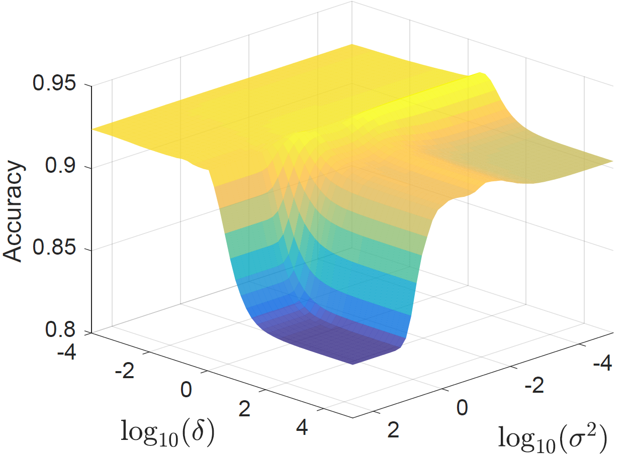
Figure 1: Accuracy of our algorithm on OSR dataset (attribute 3) with respect to varying hyperparameters $\sigma^{2}$ and $\delta$.

For joint diffusion, we set an upper bound $T_{2}$ on the number of steps in each $\mathbf{f}$- and $B$-diffusion process, and terminate the iterations immediately when the validation accuracy (for $\mathbf{f}$-diffusion) or alignment score (for $B$-diffusion) does not increase. These two processes alternate until the joint iteration number meets the upper bound $T_{1}$, or the $\mathbf{f}$-validation accuracy does not improve. Our algorithm converges fairly quickly, typically within 10 iterations. We set $T_{1},T_{2}=20$ (see Algorithm 1).

3 Experiments

3.1 Design evaluation on a synthetic dataset

To gain an insight into the effectiveness of our bridge estimation approach, we constructed a toy dataset with a known task metric structure. First, we generated 12 different tasks by explicitly building their ground-truth predictors $\{\tilde{t}^{k}\}_{k=1}^{12}$: Each member is constructed as a linear function on the $100$-dimensional input space: $\tilde{t}^{k}(\mathbf{x})=\mathbf{x}^{\top}\widetilde{\mathbf{w}}^{k}$. Among the parameter vectors of 12 predictors, the last four are randomly generated (with each element sampled from the uniform distribution on $[-1,1]$) while the first 8 parameter vectors form two groups of 4 linearly depending predictors: $\widetilde{W}^{1}=[\widetilde{\mathbf{w}}^{1},\ldots,\widetilde{\mathbf{w}}^{4}]$ is obtained by multiplying a pair of randomly generated vectors of sizes $100\times 1$ and $1\times 4$, respectively. The parameters of the second group (tasks 5-8) are generated similarly. The corresponding coupled noisy observations $H_{\text{c}}=\{\mathbf{h}_{\text{c}}^{k}\}_{k=1}^{m}$ are obtained by evaluating these ground-truths on an input dataset of $n$=1,000 data points $\widetilde{X}=\{\widetilde{\mathbf{x}}_{1},\ldots,\widetilde{\mathbf{x}}_{n}\}$ and adding a mild level of noise (i.i.d. zero-mean Gaussian with standard deviation $0.2$) to the result.

Similarly, decoupled observations $H_{\text{d}}=\{\mathbf{h}_{\text{d}}^{k}\}_{k=1}^{m}$ are constructed based on task-specific feature sets $\{X^{k}:X^{k}=\{\mathbf{x}^{k}_{1},\ldots,\mathbf{x}^{k}_{n(k)}\}\}_{k=1}^{m}$ each sub-sampled from $\widetilde{X}$ ($n(k)\approx n/2$): To simulate different feature extraction operations, we applied principal component analysis with the feature dimensions varying randomly across tasks (under the condition that 95% of the total variance is retained): $X^{k}\subset e^{k}|_{\widetilde{X}}$ with $e^{k}$ being the $k$-th principal component feature extractor. Finally, the noisy predictions $H_{\text{d}}$ are obtained by constructing the least-squares parameter approximations of $H_{\text{c}}$:

$$\mathbf{w}^{k}=\mathop{\rm arg\,min}\limits_{\mathbf{w}}\sum_{i=1}^{n(k)}(\mathbf{w}^{\top}\mathbf{x}_{i}^{k}-[\mathbf{h}_{\text{c}}^{k}]_{i})^{2},$$ (18)

evaluating the resulting predictors $\{g^{k}:g^{k}(\mathbf{x})=\mathbf{x}^{\top}\mathbf{w}^{k}\}_{k=1}^{12}$ respectively on $\{X^{k}\}_{k=1}^{12}$, and adding Gaussian noise to the results. Across different feature matrices $\{X^{k}\}_{k=1}^{12}$, the source of feature instances in the first $30$ rows are shared, providing coupling labels.

For each task $k$, we used $\mathbf{h}^{k}$ as the main predictor $\mathbf{f}$ and the rest as the references constituting a total of 12 predictor combination problems. Figure 2 shows the results of the bridge estimation process. (Left) shows the metric evaluated from the coupled predictions $H_{\text{c}}$: the $k$-row of the displayed matrix shows the metric evaluations of $\mathbf{h}_{\text{c}}^{k}$ (as the main predictor) with respect to the remaining predictors (as references). This matrix can be regarded as the ground-truths for bridge estimation process. (Center) shows the metric evaluated on the decoupled predictors $H_{\text{d}}$ using the initially estimated bridge variables $B_{k\mathbf{f}}(0)$ (Eq. 15). Given the mild level of task noise (as shown in Fig. 2(left)), the initial metric evaluations on decoupled observations already well-recovered the underlying task dependence. Finally, (Right) shows the metric evaluated on the predictions denoised via the joint diffusion process. Our algorithm successfully suppressed noise and refined the underlying metric structure.

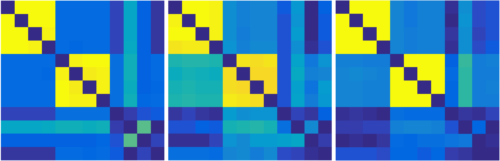
Figure 2: Example estimation of the task metric $\langle\cdot,\cdot\rangle_{M}$ (Eq. 8) from decoupled predictions $\{\mathbf{g}^{k}\}_{k=1}^{12}$. By design, tasks 1-4 and tasks 5-8 respectively form groups of strongly correlated tasks. (left) pair-wise metric evaluations from the ground-truth predictions; (center) metric estimated based on decoupled predictions using the initial bridge estimate; (right) final metric evaluations constructed via joint diffusion.

3.2 Evaluation on real datasets

We evaluate our joint manifold diffusion algorithm on seven datasets and compare its performance with four baseline algorithms. Each entry in these datasets is assigned with multiple ground-truth attributes and therefore, predicting the relative strengths of these attributes constitutes multiple predictor combination problems: For each target attribute, our algorithm refines the corresponding predictor based on the remaining predictors as references.

3.2.1 Baseline methods

A) Ind: The first baseline algorithm (Ind) evaluates and selects the best predictor per dataset, per attribute from among deep neural networks (DNNs[24]), and linear and nonlinear rank support vector machines (RankSVMs[17]) based on validation accuracy. For all experiments, the baseline algorithms were trained based on pair-wise rank labels extracted from 200 training data points. For given training inputs $X=\{\mathbf{x}_{1},\ldots,\mathbf{x}_{n}\}$ and pair-wise rank labels $\{(i(1),j(1)),\ldots,(i(l),j(l))\}$, the linear RankSVM ($f(\mathbf{x})=\mathbf{w}^{\top}\mathbf{x}$) minimizes the regularized rank energy:

$$\mathcal{E}^{S}(f)=\sum_{k=1}^{l}L([\mathbf{x}_{i(k)},\mathbf{x}_{j(k)}],f)+\lambda^{S}\|\mathbf{w}\|^{2},$$ (19)

where the margin-based rank loss $L$ is defined as

$$L([\mathbf{x}_{i},\mathbf{x}_{j}],f)=\left(\max(1-(f(\mathbf{x}_{i})-f(\mathbf{x}_{j})),0)\right)^{2}.$$ (20)

The regularization hyperparameter $\lambda^{S}\geq 0$ is tuned based on the accuracy on a separate validation set of the same size as the training set. For non-linear RankSVMs, we use a Gaussian kernel $k(\mathbf{x},\mathbf{x}^{\prime})=\exp\left(-\|\mathbf{x}-\mathbf{x}^{\prime}\|^{2}/\sigma^{2}_{S}\right)$ with a scale hyperparameter $\sigma^{2}_{S}>0$. In this case, the parameter norm $\|\mathbf{w}\|^{2}$ in Eq. 19 is replaced by the RKHS norm corresponding to $k$: $\|\mathbf{w}\|^{2}_{k}$.

B) TPC: The second baseline uses Kim et al.’s test-time predictor combination approach (TPC) [10]. This algorithm was originally developed for regression but adapting it to ranking using rank loss $L$ is straightforward. Both TPC and our algorithm require the initial main rank predictor $\mathbf{f}(0)$ and reference predictors $\{\mathbf{g}^{k}\}_{k=1}^{m}$ as inputs, which we obtain from Ind.

C) MTL¹: The last two baselines (MTL¹ and MTL²) implement adaptations of two existing multi-task learning algorithms. MTL¹ is based on Evgeniou and Pontil’s approach of penalizing the pair-wise parameter deviations [6]. Adapted to test time combination setting, MTL¹ minimizes

$$\mathcal{L}_{\text{\emph{MTL}${}^{1}$}}(f) =\sum_{k=1}^{l}L([\mathbf{x}_{i(k)},\mathbf{x}_{j(k)}],f)$$

$$+\lambda^{S}\|\mathbf{w}\|^{2}+\lambda^{2}\sum_{k=1}^{m}W_{k}\|\mathbf{w}-\mathbf{w}^{k}\|^{2}$$ (21)

where the weight parameters $\{W_{k}\}_{k=1}^{m}$ are defined similarly as in our task graph Laplacian (Eq. 5): $W_{k}=\exp(-\|\mathbf{w}-\mathbf{w}^{k}\|^{2}/\sigma^{2}_{\mathbf{w}})$. The hyperparameters $\lambda^{S}$, $\lambda^{2}$, and $\sigma^{2}_{\mathbf{w}}$ are tuned based on a validation set. Similarly to RankSVM, MTL¹ can also construct non-linear predictors using Gaussian kernels (with hyperparameter $\sigma^{2}_{S}$).

D) MTL² adapts Pentina et al.’s curriculum learning approach [19], which penalizes the deviation of the main predictor parameter $\mathbf{w}$ from a single best reference predictor $\mathbf{w}^{k}$. Pentina et al.’s original algorithm uses a bound on the generalization accuracy to select the reference predictor, which is not directly applicable to our rank learning problem. Instead, validation accuracy is used to select the reference.

For all datasets, we ran ten experiments with different training and validation set configurations and report the average results.

3.2.2 Datasets

A) Public Figure Face (PubFig) dataset contains 800 images from 8 random identities [17]. Our goal is to estimate a linear ordering of database images based on the relative strengths of each of 11 different facial attributes (Masculine-looking, White, Young, Smiling, Chubby, Visible-forehead, Bushy-eyebrows Narrow-eyes, Pointy-nose, Big-lips, and Round-face).

B) Outdoor Scene Recognition (OSR) dataset provides 2,688 images of 8 scene categories and 6 attributes [17].

We use a combination of GIST features and color histograms for PubFig and GIST features for OSR. The attribute rank labels are constructed from the category labels as provided by the authors of [17]. For each attribute, we improve the corresponding predictor using the predictors of the remaining attributes as references.

C) Shoes dataset contains 14,658 images of 10 categories and 10 attributes [11]. We use a combination of GIST features and color histograms provided by the authors of [11]. Our goal is to estimate the attribute rankings similarly to PubFig and OSR settings. However, here the datasets for the main and reference predictors are disjoint and we explicitly estimate the bride variables using additional 200 paired instances. As in this case TPC is not applicable, we compare with MTL¹ and MTL².

D) Cal7 dataset contains 1,474 images of 7 categories (Face, Motorbikes, Dolla-Bill, Garfield, Snoopy, Stop-Sign, and Windor-Chair) as a subset of Caltech-101 dataset [7]. The dataset provides five different feature representations per image: wavelet, Gabor, CENTRIST, HOG, GIST, and LBP features [14]. The goal is to estimate a linear database ordering according to the category of each entry. For each single feature, we configured a corresponding main prediction task and constructed reference predictors using the remaining features. For each experiment, two disjoint feature sets for the main and reference predictors, respectively are prepared (roughly, half of the dataset was allocated for the main and the rest were allocated for references) representing the scenario where multiple predictions are generated based on heterogeneous, decoupled feature observations. To estimate the bridge variables, we use 200 coupled data instances as a sample from the joint distribution $P(f,g^{1},\ldots,g^{m})$. As the predictor variables are decoupled across tasks, TPC is not applicable. Further, since the respective feature spaces and the corresponding predictors are heterogeneous, (adaptations of) classical parametric MTL approaches cannot be directly applied. Therefore, we compare our algorithm with only independent baselines (Ind).

E) NUS-WIDE-Object (NUS) dataset contains 30,000 images of 31 categories [3]. We use color histogram, color moments, color correlation, edge distribution and wavelet features as provided by the authors of [3] and [14].

F) Handwritten digits (HW) dataset provides 6 different feature representations of 2,000 handwritten digits, each represented by Fourier coefficients, profile correlations, Karhunen-Loève coefficients, pixel averages in $2\times 3$ windows, Zernike moment and morphological features [2].

Experimental settings for NUS and HW are identical to Cal7. We use 200 paired data instances to learn bridge variables.

G) Animals With Attributes (AWA) dataset contains 30,475 images of 50 animal categories. We use the SURF, SIFT and PHOG histograms and the features extracted by pre-trained DeCAF [5] and VGG19 [21] networks as provided by the authors of [13]. The experimental setting is similar to those of Cal7-HW except that, here we explicitly pair all data points across tasks enabling the application of TPC. This toy setting constitutes the ideal case where all reference predictors are inherently relevant in refining the main predictor and it enables us to verify the correct operation of TPC and our approach.

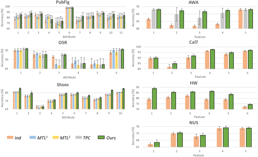
Figure 3: Average accuracy of different ranking algorithms (over 10 different training and test set configurations. Ind: best baseline independent predictors; MTL¹ and MTL²: adaptations of existing MLT algorithms ([6] and [19], respectively); TPC: Kim et al.’s test-time predictor combination algorithm [10]. The length of each error bar corresponds to twice the standard deviation.

3.2.3 Results

Figure 3 summarizes the results. While not all target attributes show marked improvements, TPC and our algorithm consistently improve upon or are on par with Ind. Comparing TPC and ours, the performances are almost identical on OSR. For PubFig, the two algorithms demonstrated the complementary strengths across different target attributes, while our algorithm achieves higher average accuracy. The corresponding results on AWA are notably different: While TPC already achieves better results than the baseline Ind, our algorithm further improves accuracy by a large margin. In addition, by virtue of the fast Eigen-decomposition-based approach (Eq. 10) the runtime of our algorithm is around 20$\times$ shorter than TPC: For AWA with 30,475 images, our algorithm took around 0.2 seconds for the entire combination process. As TPC requires fully coupled predictor evaluations, it cannot be applied to Cal7, NUS, and HW datasets, in which our algorithm continues to outperform Ind. For these datasets, our algorithm demonstrates even better performance than the best individual task predictors, which demonstrates the utility of combining predictors across multiple features.

The two multi-task learning adaptations MTL¹ and MTL² to the test-time combination setting also showed measurable performance improvement over Ind. In particular, they achieved the highest average accuracy on target attributes 2, 4, and 5 of the OSR dataset. On the other hand, for PubFig and Shoes, our algorithm constantly outperformed these algorithms demonstrating complementary strengths. As both MTL¹ and MTL² require the parametric forms of all predictors to be shared across different tasks, it is not straightforward to apply these algorithms when different tasks use heterogeneous features (Cal7, NUS, and HW datasets).

4 Conclusion

In this paper, we have presented a new algorithm improving a given task predictor by combining multiple reference predictors, each constructed from the respective tasks. Conventional approaches require either all task predictor’s known and shared parametric forms or multiple predictors’ evaluation on a single fixed dataset. We address these limitations by formulating the problem as a non-parametric task dependence estimation and by a robust joint diffusion process that automatically couples the predictors of disjoint data instances. This not only facilitates a new (decoupled, parameter-free) predictor combination application but also significantly improves the accuracy and run-time over existing algorithms when applied to challenging relative attributes ranking datasets.

Our manifold structure (Eq. 1) and metric therein (Eqs. 2–3) are directly aligned with the case when the predictor outputs are one-dimensional (e.g. ranking and regression problems). When the output space is multi-dimensional (e.g. multi-class classification), our metric structure needs changing to align predictions of different dimensions. We expect that this can be done by calculating canonical correlations between the input pairs, but it would involve non-trivial modifications.

Identifying data coupling across heterogeneous domains is a challenging problem. This problem arises in the predictor combination setting where different predictors are evaluated on data instances sampled from multiple heterogeneous domains. We attempted to address this challenge by estimating soft couplings via a joint diffusion process propagating a small set of coupled data points. An alternative possibility that we have not explored in this work is to consider recent label-free set pairing approaches, e.g. instantiated using cyclic GANs [26]. This type of approach is not immediately applicable to our setting as they do not generate explicit pairings and, therefore, would require modifying the entire task dependence measure and the corresponding denoising process. Future work should explore this possibility.

References

- [1] A. Argyriou, T. Evgeniou, and M. Pontil. Convex multi-task feature learning. Machine Learning, 73(3), 2008.
- [2] C. L. Blake and C. J. Merz. UCI repository of machine learning databases, 1998. https://archive.ics.uci.edu/ml.
- [3] T. Chua, J. Tang, R. Hong, H. Li, Z. Luo, and Y. Zheng. NUS-WIDE: a real-world web image database from National University of Singapore. In ACM CIVR, pages 48:1–48:9, 2009.
- [4] C. Cortes, M. Mohri, and A. Rostamizadeh. Algorithms for learning kernels based on centered alignment. JMLR, 13:795–828, 2012.
- [5] J. Donahue, Y. Jia, O. Vinyals, J. Hoffman, N. Zhang, E. Tzeng, and T. Darrell. DeCAF: a deep convolutional activation feature for generic visual recognition. In ICML, pages 647–655, 2014.
- [6] T. Evgeniou and M. Pontil. Regularized multi–task learning. In KDD, pages 109–117, 2004.
- [7] L. Fei-Fei, R. Fergus, and P. Perona. Learning generative visual models from few training examples: An incremental bayesian approach tested on 101 object categories. Computer Vision and Image Understanding, 106(1):59–70, 2007.
- [8] P. Gong, J. Ye, and C. Zhang. Robust multi-task feature learning. In KDD, pages 895–903, 2012.
- [9] M. Hein and M. Maier. Manifold denoising. In NIPS, pages 561–568, 2007.
- [10] K. I. Kim, J. Tompkin, and C. Richardt. Predictor combination at test time. In ICCV, pages 3553–3561, 2017.
- [11] A. Kovashka, D. Parikh, and K. Grauman. Whittlesearch: Image search with relative attribute feedback. In CVPR, pages 2973–2980, 2012.
- [12] A. Kumar and H. Daumé III. Learning task grouping and overlap in multi-task learning. In ICML, pages 1383–1390, 2012.
- [13] C. H. Lampert, H. Nickisch, and S. Harmeling. Learning to detect unseen object classes by between-class attribute transfer. In CVPR, pages 951–958, 2009.
- [14] Y. Li, F. Nie, H. Huang, and J. Huang. Large-scale multi-view spectral clustering via bipartite graph. In Proc. AAAI, pages 2750–2756, 2015.
- [15] Y. Lu, L. Wang, J. Lu, J. Yang, and C. Shen. Multiple kernel clustering based on centered kernel alignment. Pattern Recogn., 47:3656–3664, 2014.
- [16] Y. Luo, D. Tao, B. Geng, C. Xu, and S. J. Maybank. Manifold regularized multitask learning for semi-supervised multilabel image classification. IEEE TIP, 22(2):523–536, 2013.
- [17] D. Parikh and K. Grauman. Relative attributes. In ICCV, pages 503–510, 2011.
- [18] A. Passos, P. Rai, J. Wainer, and H. Daumé III. Flexible modeling of latent task structures in multitask learning. In ICML, pages 1103–1110, 2012.
- [19] A. Pentina, V. Sharmanska, and C. H. Lampert. Curriculum learning of multiple tasks. In CVPR, pages 5492–5500, 2015.
- [20] I. Redko and Y. Bennani. Kernel alignment for unsupervised transfer learning,. In arXiv:1610.06434v1, 2016.
- [21] K. Simonyan and A. Zisserman. Very deep convolutional networks for large-scale image recognition. In ICLR, page arXiv:1409.1556, 2015.
- [22] B. Wang and Z. Tu. Sparse subspace denoising for image manifolds. In CVPR, pages 468–475, 2013.
- [23] Y. Yan, E. Ricci, R. Subramanian, G. Liu, and N. Sebe. Multitask linear discriminant analysis for view invariant action recognition. IEEE TIP, 23(12):5599–5611, 2014.
- [24] X. Yang, T. Zhang, C. Xu, S. Yan, M. S. Hossain, and A. Ghoneim. Deep relative attributes. IEEE T-MM, 18(9):1832–1842, 2016.
- [25] L. W. Zhong and J. T. Kwok. Convex multitask learning with flexible task clusters. In ICML, pages 49–56, 2012.
- [26] J.-Y. Zhu, T. Park, P. Isola, and A. A. Efros. Unpaired image-to-image translation using cycle-consistent adversarial networks. In ICCV, pages 2223–2232, 2017.