DeepSphere: towards an equivariant graph-based spherical CNN

Abstract

Spherical data is found in many applications. By modeling the discretized sphere as a graph, we can accommodate non-uniformly distributed, partial, and changing samplings. Moreover, graph convolutions are computationally more efficient than spherical convolutions. As equivariance is desired to exploit rotational symmetries, we discuss how to approach rotation equivariance using the graph neural network introduced in Defferrard et al. (2016). Experiments show good performance on rotation-invariant learning problems. Code and examples are available at https://github.com/SwissDataScienceCenter/DeepSphere.

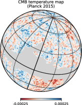
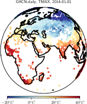
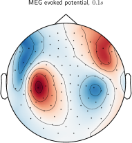
Figure 1: Examples of intrinsically spherical data: (left) the cosmic microwave background (CMB) temperature from Planck Collaboration (2016), (middle) daily maximum temperature from the Global Historical Climatology Network (GHCN),(right) brain activity recorded through magnetoencephalography (MEG).For those examples, a rigid full-sphere pixelization is not ideal: the Milky Way’s galactic plane masks observations, brain activity is measured on the scalp only, and the position and density of weather stations is arbitrary and changes over time. Graphs can faithfully and efficiently represent sampled spherical data by placing vertices where data has been measured.

1 Introduction

Graphs have long been used as models for discretized manifolds: for example to smooth meshes (Taubin et al., 1996), reduce dimensionality (Belkin & Niyogi, 2003), and, more recently, to process signals (Shuman et al., 2013). Along Euclidean spaces, the sphere is one of the most commonly encountered manifold: it is notably used to represent omnidirectional images, global planetary data (in meteorology, climatology, geology, geophysics, etc.), cosmological observations, and brain activity measured on the scalp (see figure 4). Spherical convolutional neural networks (CNNs) have been developed to work with some of these modalities (Cohen et al., 2018; Perraudin et al., 2018; Frossard & Khasanova, 2017; Su & Grauman, 2017; Coors et al., 2018; Jiang et al., 2019).

Spherical data can be seen as a continuous function that is sampled at discrete locations. As it is impossible to construct a regular discretization of the sphere, there is no perfect spherical sampling. Schemes have been engineered for particular applications and come with trade-offs (Gorski et al., 2005; Doroshkevich et al., 2005). However, while sampling locations can be precisely controlled in some cases (like the CMOS sensors of an omni-directional camera), sensors might in general be non-uniformly distributed, cover only part of the sphere, and move (see figure 4). Modeling the sampled sphere as a discrete graph has the potential to faithfully and efficiently represent sampled spherical data by placing vertices where data has been measured: no need to handle missing data or to interpolate to some predefined sampling, and no waste of memory or precision due to over- or under-sampling. Graph-based spherical CNNs have been proposed in Frossard & Khasanova (2017) and Perraudin et al. (2018). Moreover, graph convolutions have a low computational complexity of $\mathcal{O}(N_{pix})$, where $N_{pix}$ is the number of considered pixels. Methods based on proper spherical convolutions, like Cohen et al. (2018) and Esteves et al. (2017), cost $\mathcal{O}(N_{pix}^{2/3})$ operations.

Finally, like classical 2D CNNs are equivariant to translations, we want spherical CNNs to be equivariant to 3D rotations (Cohen & Welling, 2016; Kondor & Trivedi, 2018). A rotation-equivariant CNN detects patterns regardless of how they are rotated on the sphere: it exploits the rotational symmetries of the data through weight sharing. Realizing that, spheres can be used to support data which does not intrinsically live on a sphere but have rotational symmetries (Cohen et al., 2018; Esteves et al., 2017, for 3D objects and molecules). In this contribution we present DeepSphere (Perraudin et al., 2018), a spherical neural network leveraging graph convolution for its speed and flexibility. Furthermore, we discuss the rotation equivariance of graph convolution on the sphere.

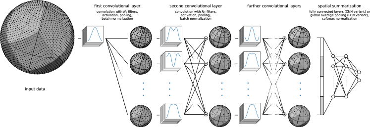
Figure 2: Example architecture. Global tasks need a spatial summarization: the FCN variant is rotation invariant (and accepts inputs of varying sizes), while the CNN variant is not. Dense tasks (when the output lives on the sphere, like segmentation) are rotation equivariant.

2 Method

Our method relies on the graph signal processing framework (Shuman et al., 2013), which highly relies on the spectral properties of the graph Laplacian operator. In particular, the Fourier transform is defined as the projection of the signal on the eigenvectors of the Laplacian, and the graph convolution as a multiplication in the Fourier domain. It turns out that the graph convolution can be accelerated by being performed directly in the vertex domain (Hammond et al., 2011).

DeepSphere leverages graph convolutions to achieve the following properties: (i) computational efficiency, (ii) adaptation to irregular sampling, and (iii) close to rotation equivariance. An example architecture is shown in figure 2. The main idea is to model the discretised sphere as a graph of connected pixels: the length of the shortest path between two pixels is an approximation of the geodesic distance between them. We use the graph CNN formulation introduced in (Defferrard et al., 2016), and a pooling strategy that exploits a hierarchical pixelisation of the sphere to analyse the data at multiple scales. The current implementation of DeepSphere relies on the Hierarchical Equal Area isoLatitude Pixelisation (HEALPix) (Gorski et al., 2005), a popular sampling used in cosmology and astrophysics. See Perraudin et al. (2018) for details. DeepSphere is, however, easily used with other samplings as only two elements depend on it: (i) the choice of neighboring pixels when building the graph, and (ii) the choice of parent pixels when building the hierarchy.

The flexibility of modeling the data domain with a graph allows one to easily model data that spans only a part of the sphere, or data that is not uniformly sampled. Furthermore, using a $k$-nearest neighbors graph, the convolution operation costs $\mathcal{O}(N_{pix})$ operations. This is the lowest possible complexity for a convolution without approximations. Nevertheless, while the graph framework offers great flexibility, its ability to faithfully represent the underlying sphere highly depends on the sampling locations and the graph construction. This should not be neglected since the better the graph represents the sphere, the closer to rotation equivariant the graph convolution will be.

3 Harmonics and equivariance

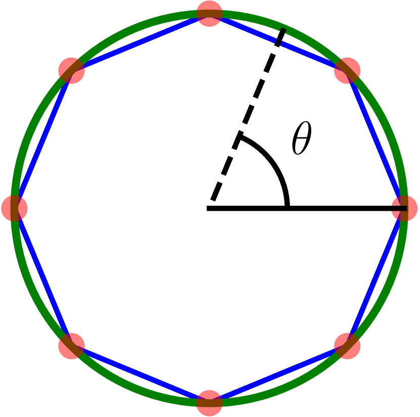
Figure 3: circle $\mathcal{C}^{1}$ (green), regular samples and graph vertices (red), graph edges (blue).

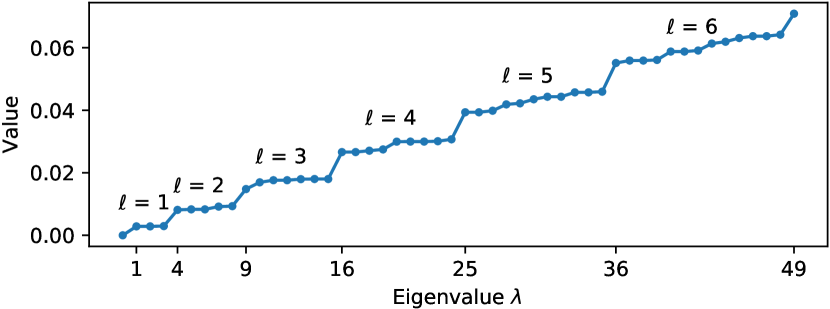
Figure 4: The eigenvalues ${\bm{\Lambda}}$ of the graph Laplacian ${\bm{L}}={\bm{U}}{\bm{\Lambda}}{\bm{U}}^{\intercal}$ are clearly organized in groups. Each group corresponds to a degree $\ell$ of the spherical harmonics. Each degree has $2\ell+1$ orders.

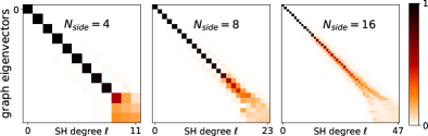
Figure 5: Correspondence between the subspaces spanned by the graph Fourier basis and the spherical harmonics. The eigenvectors ${\bm{U}}=[{\bm{u}}_{1},\dots,{\bm{u}}_{N_{pix}}]$ of the graph Laplacian ${\bm{L}}={\bm{U}}{\bm{\Lambda}}{\bm{U}}^{\intercal}$, which form the Fourier basis, clearly resemble the spherical harmonics. The first 8 are shown on the left. To quantify the correspondence, we compute the power spectral density (PSD) of each eigenvector with the SHT. Second, as there is $2\ell+1$ spherical harmonics for each degree $\ell$, we sum the contributions of the corresponding $2\ell+1$ eigenvectors. The matrices on the right show how the subspaces align: the Fourier basis spans the same subspaces as the spherical harmonics in the low frequencies, and the eigenvectors leak towards adjacent frequency bands at higher frequencies. The graph Fourier basis aligns at higher frequencies as the resolution ($N_{pix}=12N_{side}^{2}$) increases.

Both the graph and the spherical convolutions can be expressed as multiplications in a Fourier domain. As the spectral bases align, the two operations become similar. Hence, the equivariance property of the spherical convolution carries out to the graph convolution.

Known case: the circle $\mathcal{C}^{1}$.

Let $\theta\in[0,2\pi[$ be a parametrization of each point $(\cos\theta,\sin\theta)$ of $\mathcal{C}^{1}$. The eigenfunctions of the Laplace-Beltrami operator of $\mathcal{C}^{1}$ are $u_{\ell}(\theta)=e^{i\theta m\ell}$, for $\ell\in\mathbb{N}$ and $m\in\{-1,1\}$. Interestingly, for a regular sampling of $\mathcal{C}^{1}$ (shown in figure 4), the sampled eigenfunctions turn out to be the discrete Fourier basis. That is, the harmonic decomposition of a discretized function on the circle can be done using the well-known discrete Fourier transform (DFT). Moreover, the graph Laplacian of the sampled circle is diagonalized by the DFT basis, as all circulant matrices have complex exponentials as eigenbases Strang (1999). Hence, for $\mathcal{C}^{1}$, it can be verified, under mild assumptions, that the graph convolution is equivariant to translation (Perraudin & Vandergheynst, 2017, section 2.2 and equation 3). More generally, higher dimensional circles such as the torus $\mathcal{C}^{2}$ also have a circulant Laplacian and an equivariant convolution. The above does however not hold for irregular samplings: the more irregular the sampling, the further apart the graph Fourier basis will be to the sampled eigenfunctions.

Analysis of the graph Laplacian used in DeepSphere.

As there is no regular sampling of the sphere, we cannot have a similar reasoning as we had for the circle. We can however perform a harmonic analysis to empirically assess how similar the graph and the spherical convolutions are. The graph Laplacian eigenvalues, shown in figure 4, are clearly organized in frequency groups of $2\ell+1$ orders for each degree $\ell$. These blocks correspond to the different eigenspaces of the spherical harmonics. We also show the correspondence between the subspaces spanned by the graph Fourier basis and the spherical harmonics in figure 5. For example with $N_{side}=4$, we observe a good alignment for $\ell\leq 8$: the graph convolution will be equivariant to rotations for low frequency filters. The imperfections are likely due to the small irregularities of the HEALPix sampling (varying number of neighbors and varying distances between vertices). Furthermore, a follow-up study is underway to optimally construct the graph. We also hope to get a proof of equivalence or convergence.

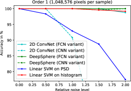
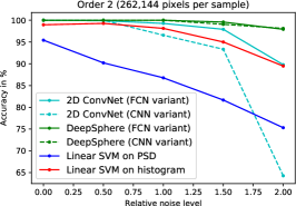
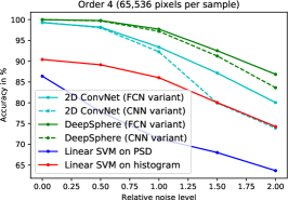
Figure 6: Classification accuracies. The difficulty of the task depends on the level of noise and the size of a sample (that is, the number of pixels that constitute the sample to classify). Order $o=1$ corresponds to samples which area is $\frac{1}{12}=8.1\%$ of the sphere ($\approx 1\times 10^{6}$ pixels), order $o=2$ to $\frac{1}{12\times 2^{2}}=2.1\%$ ($\approx 260\times 10^{3}$ pixels), and order $o=4$ to $\frac{1}{12\times 4^{2}}=0.5\%$ ($\approx 65\times 10^{3}$ pixels). The FCN variant of DeepSphere beats the CNN variant by being invariant to rotation. Both variants largely beat the 2D ConvNet and the two SVM baselines.

4 Experiments

Setup.

The performance of DeepSphere is demonstrated on a discrimination problem: the classification of cosmological convergence maps into two model classes. Details about the experimental setup can be found in Perraudin et al. (2018). Code to reproduce the results is in the git repository.

We propose two architectures: the “CNN variant”, where convolutional layers are followed by dense layers, and the “FCN variant”, where convolutional layers are followed by global average pooling. The FCN variant is rotation invariant to the extent that the convolution is rotation equivariant.

Baselines.

DeepSphere is first compared against two simple yet powerful cosmological baselines, based on features that are (i) the power spectral densities (PSD) of maps, and (ii) the histogram of pixels in the maps (Patton et al., 2017). DeepSphere is further compared to a classical CNN for 2D Euclidean grids, as in (Krachmalnicoff & Tomasi, 2019). To be fed into the 2D ConvNet, partial spherical signals are transformed into flat images. DeepSphere and the 2D ConvNet have the same number of trainable parameters.

Results.

Figure 6 summaries the results. Overall, DeepSphere performs best with a gap that widens as the problem gets more difficult. The FCN variant outperforms the CNN variant as it exploits the rotational symmetry of the task (explained by the cosmological principle of homogeneity and isotropy). The 2D ConvNet fairs in-between the SVMs and DeepSphere. Lower performance is thought to be due to a lack of rotation equivariance, and to the geometric distortion introduced by the projection, which the NN has to learn to compensate for.

Acknowledgments

We thank Pierre Vandergheynst for advice and helpful discussions, and Andreas Loukas for having processed the raw GHCN data. The Python Graph Signal Processing package (PyGSP) (Defferrard et al., ) was used to build graphs, compute the Laplacian and Fourier basis, and perform graph convolutions.

References

- Belkin & Niyogi (2003) Mikhail Belkin and Partha Niyogi. Laplacian eigenmaps for dimensionality reduction and data representation. Neural computation, 15(6):1373–1396, 2003.
- Cohen & Welling (2016) Taco Cohen and Max Welling. Group equivariant convolutional networks. In International conference on machine learning, pp. 2990–2999, 2016.
- Cohen et al. (2018) Taco S Cohen, Mario Geiger, Jonas Koehler, and Max Welling. Spherical cnns. arXiv:1801.10130, 2018.
- Coors et al. (2018) Benjamin Coors, Alexandru Paul Condurache, and Andreas Geiger. Spherenet: Learning spherical representations for detection and classification in omnidirectional images. In European Conference on Computer Vision, 2018.
- (5) Michaël Defferrard, Lionel Martin, Rodrigo Pena, and Nathanaël Perraudin. Pygsp: Graph signal processing in python. URL https://github.com/epfl-lts2/pygsp/.
- Defferrard et al. (2016) Michaël Defferrard, Xavier Bresson, and Pierre Vandergheynst. Convolutional neural networks on graphs with fast localized spectral filtering. In Advances in Neural Information Processing Systems, pp. 3844–3852, 2016.
- Doroshkevich et al. (2005) AG Doroshkevich, PD Naselsky, Oleg V Verkhodanov, DI Novikov, VI Turchaninov, ID Novikov, PR Christensen, and L-Y Chiang. Gauss–legendre sky pixelization (glesp) for cmb maps. International Journal of Modern Physics D, 14(02):275–290, 2005.
- Esteves et al. (2017) Carlos Esteves, Christine Allen-Blanchette, Ameesh Makadia, and Kostas Daniilidis. Learning so(3) equivariant representations with spherical cnns. arXiv:1711.06721, 2017.
- Frossard & Khasanova (2017) P. Frossard and R. Khasanova. Graph-based classification of omnidirectional images. In 2017 IEEE International Conference on Computer Vision Workshops (ICCVW), pp. 860–869, Oct 2017.
- Gorski et al. (2005) Krzysztof M Gorski, Eric Hivon, AJ Banday, Benjamin D Wandelt, Frode K Hansen, Mstvos Reinecke, and Matthia Bartelmann. Healpix: a framework for high-resolution discretization and fast analysis of data distributed on the sphere. The Astrophysical Journal, 622(2):759, 2005.
- Hammond et al. (2011) David K Hammond, Pierre Vandergheynst, and Rémi Gribonval. Wavelets on graphs via spectral graph theory. Applied and Computational Harmonic Analysis, 30(2):129–150, 2011.
- Jiang et al. (2019) Chiyu Jiang, Jingwei Huang, Karthik Kashinath, Philip Marcus, Matthias Niessner, et al. Spherical cnns on unstructured grids. arXiv preprint arXiv:1901.02039, 2019.
- Kondor & Trivedi (2018) Risi Kondor and Shubhendu Trivedi. On the generalization of equivariance and convolution in neural networks to the action of compact groups. arXiv:1802.03690, 2018.
- Krachmalnicoff & Tomasi (2019) Nicoletta Krachmalnicoff and Maurizio Tomasi. Convolutional neural networks on the healpix sphere: a pixel-based algorithm and its application to cmb data analysis. arXiv preprint arXiv:1902.04083, 2019.
- Patton et al. (2017) K. Patton, J. Blazek, K. Honscheid, E. Huff, P. Melchior, A. J. Ross, and E. Suchyta. Cosmological constraints from the convergence 1-point probability distribution. Monthly Notices of the Royal Astronomical Society, 472:439–446, November 2017.
- Perraudin & Vandergheynst (2017) Nathanaël Perraudin and Pierre Vandergheynst. Stationary signal processing on graphs. IEEE Transactions on Signal Processing, 65(13):3462–3477, 2017.
- Perraudin et al. (2018) Nathanaël Perraudin, Michaël Defferrard, Tomasz Kacprzak, and Raphael Sgier. Deepsphere: Efficient spherical convolutional neural network with healpix sampling for cosmological applications. arXiv preprint arXiv:1810.12186, 2018.
- Planck Collaboration (2016) Planck Collaboration. Planck 2015 results. I. Overview of products and scientific results. Astronomy & Astrophysics, 594:A1, September 2016.
- Sgier et al. (2018) R. Sgier, A. Réfrégier, A. Amara, and A. Nicola. Fast Generation of Covariance Matrices for Weak Lensing. arxiv:1801.05745, January 2018.
- Shuman et al. (2013) David I Shuman, Sunil K Narang, Pascal Frossard, Antonio Ortega, and Pierre Vandergheynst. The emerging field of signal processing on graphs: Extending high-dimensional data analysis to networks and other irregular domains. IEEE Signal Processing Magazine, 30(3):83–98, 2013.
- Strang (1999) Gilbert Strang. The discrete cosine transform. SIAM review, 41(1):135–147, 1999.
- Su & Grauman (2017) Yu-Chuan Su and Kristen Grauman. Learning spherical convolution for fast features from 360 imagery. In Advances in Neural Information Processing Systems, pp. 529–539, 2017.
- Taubin et al. (1996) Gabriel Taubin, Tong Zhang, and Gene Golub. Optimal surface smoothing as filter design. In European Conference on Computer Vision, pp. 283–292. Springer, 1996.