Abstract

In [1] an effective algorithm for inverting polynomial automorphisms was proposed. Also the class of Pascal finite polynomial automorphisms was introduced. Pascal finite polynomial maps constitute a generalization of exponential automorphisms to positive characteristic. In this note we explore properties of the algorithm while using Segre homotopy and reductions modulo prime number. We give a method of retrieving an inverse of a given polynomial automorphism $F$ with integer coefficients form a finite set of the inverses of its reductions modulo prime numbers. Some examples illustrate effective aspects of our approach.

1 Introduction

Let $K$ be a field and let $F=(F_{1},\ldots,F_{n}):K^{n}\rightarrow K^{n}$ be a polynomial map. $F$ is invertible over $K$ if there exists a polynomial mapping $G:K^{n}\rightarrow K^{n}$ such that $F\circ G=Id$ and $G\circ F=Id$. Study of invertible polynomial mappings is related to the famous Jacobian Conjecture, which asks if every polynomial mapping such that its jacobian is nonzero constant is invertible with polynomial inverse. Many results concerning polynomial automorphisms are formulated for an arbitrary field $K$, but the case of a field of characteristic zero is the one discussed most often. However after reducing coefficients of $F\in\mathbb{Z}[X]^{n}$ modulo given prime number one can consider it over finite field $\mathbb{F}_{p}$. Results concerning this approach can be found for example in [9], [10].

In [1] we described an algorithm which for a given $F\in K[X]^{n}$ over an arbitrary field $K$ constructs recursively a sequence of polynomial maps. We define an endomorphism $\sigma_{F}$ of $K[X]^{n}$ by $\sigma_{F}(P)=P\circ F$ and a $\sigma_{F}$-derivation $\Delta_{F}$ on $K[X]^{n}$ by $\Delta_{F}(P)=\sigma_{F}(P)-P$. Following Maple environment commands we use term lower degree instead of an order of vanishing of a polynomial. We consider $F\in K[X]^{n}$ of the form

$$\left\{\begin{array}[]{lll}F_{1}(X_{1},\ldots,X_{n})&=&X_{1}+H_{1}(X_{1},\ldots,X_{n})\\ &\vdots&\\ F_{n}(X_{1},\ldots,X_{n})&=&X_{n}+H_{n}(X_{1},\ldots,X_{n}),\end{array}\right.$$ (1)

where $H_{i}(X_{1},\ldots,X_{n})$ is a polynomial in $X_{1},\ldots,X_{n}$ of degree $D_{i}$ and lower degree $d_{i}$, with $d_{i}\geq 2$, for $i=1,\ldots,n$. Let $d=\min d_{i},D=\max D_{i}$. Then we consider the sequence $P_{l}=(P_{l}^{1},\ldots,P_{l}^{n})$ of polynomial maps in $K[X]^{n}$ defined by $P_{l}=\Delta^{l}_{F}(Id)$, where $Id(X)=X$ and $\Delta^{l}_{F}$ denotes $\Delta_{F}\circ\stackrel{{\scriptstyle l}}{{\dots}}\circ\Delta_{F}$. The class of polynomial automorphisms for which the algorithm stops has been distinguished. Polynomial map $F:K^{n}\rightarrow K^{n}$ is called Pascal finite if there exists $m$ such that $P_{m}=0$. Then $F$ is invertible and the inverse map $G$ of $F$ is given by

$$G(X)=\sum_{l=0}^{m-1}(-1)^{l}P_{l}(X)$$ (2)

(see [1], corollary 2.1). Pascal finite automorphisms are roots of a polynomial of the form $P(X)=(X-1)^{m}$. In [2] we discussed their properties. They are natural generalization of exponential automorphisms to positive characteristic.

In this paper we consider polynomial maps over $\mathbb{Q}$. Those can be transformed into maps with coefficients in $\mathbb{Z}$ by using Segre homotopy also known as denominators clearing procedure. Using clearing map Connel and van den Dries proved (see [5], theorem 1.5 or [6], proposition 1.1.19) that if there is a counterexample to the Jacobian Conjecture $h:\mathbb{C}^{m}\rightarrow\mathbb{C}^{m}$, then for some $n>m$ there is a counterexample $f:\mathbb{C}^{n}\rightarrow\mathbb{C}^{n}$ with coefficients in $\mathbb{Z}$. In fact Jacobian Conjecture over $\mathbb{C}$ is equivalent to the Jacobian Conjecture over $\mathbb{Z}$ (see [6], proposition 1.1.12). That is why one can be interested in studying maps with integer coefficients. We discuss behaviour of the algorithm while using Segre homotopy. After that we perform reduction modulo prime number $p$ and apply the algorithm proposed in [1] in order to find an inverse of a reduced map. We explore a method of retrieving an inverse of a given polynomial automorphism $F\in\mathbb{Z}[X]^{n}$ from a finite set of the inverses of its reductions modulo prime numbers.

Below we recall the main result of [1] (see theorem 3.1) which formulates an equivalent condition to invertibility of a polynomial map and explains how Pascal finite automorphisms admit an algorithmic treatment. This theorem allows to to check if a given polynomial map is invertible and to find an inverse of a given polynomial automorphism even if it is not a Pascal finite one.

Theorem 1.

Let $F=(F_{1},\ldots,F_{n}):K^{n}\rightarrow K^{n}$ be a polynomial map of the form (1). The following conditions are equivalent:

1. $F$ is invertible.

2. For $i=1,\ldots,n$ and every $m>\frac{D^{n-1}-d_{i}}{d-1}+1$, we have

   $$\sum_{j=0}^{m-1}(-1)^{j}P^{i}_{j}(X)=G_{i}(X)+R^{i}_{m}(X),$$ (3)

   where $G_{i}(X)$ is a polynomial of degree $\leq D^{n-1}$, independent of $m$, and $R^{i}_{m}(X)$ is a polynomial satisfying $R^{i}_{m}(F)=(-1)^{m+1}P^{i}_{m}(X)$ (with lower degree $\geq(m-1)(d-1)+d_{i}>D^{n-1}$).

3. For $i=1,\ldots,n$ and $m=\lfloor\frac{D^{n-1}-d_{i}}{d-1}+1\rfloor+1$, we have

   $$\sum_{j=0}^{m-1}(-1)^{j}P^{i}_{j}(X)=G_{i}(X)+R^{i}_{m}(X).$$

   where $G_{i}(X)$ is a polynomial of degree $\leq D^{n-1}$, and $R^{i}_{m}(X)$ is a polynomial satisfying $R^{i}_{m}(F)=(-1)^{m+1}P^{i}_{m}(X)$.

Moreover the inverse $G$ of $F$ is given by

$$G_{i}(Y_{1},\ldots,Y_{n})=\sum_{l=0}^{m-1}(-1)^{l}\widetilde{P}^{i}_{l}(Y_{1},\ldots,Y_{n}),\,i=1,\ldots,n,$$ (4)

where $\widetilde{P}^{i}_{l}$ is the sum of homogeneous summands of $P^{i}_{l}$ of degree $\leq D^{n-1}$ and $m$ is an integer $>\frac{D^{n-1}-d_{i}}{d-1}+1$.

2 Segre homotopy

Let us recall the notion of a clearing map, also known as Segre homotopy (see [6] chapter 1.1 and also [4]). Let $R$ be a a commutative ring. We start with a map $F\in R[X]^{n}$ of the form (1). Then we can see $F$ as a following sum $F=F_{(1)}+F_{(2)}+\ldots$, where $F_{(i)}$ is homogeneous of degree $i$. Following the idea of Segre (see [4]) one may instead of $F$ consider a map

$$\widehat{F}(X)=t^{-1}F(tX)=X+t^{-1}H(tX)=X+\widehat{H}(X).$$

Here $t$ is a new variable and $\widehat{F}\in(R[t])[X]^{n}$. Of course for a two given maps $F$ and $L$ we have

$$\widehat{F}(X)\circ\widehat{L}(X)=t^{-1}F(tt^{-1}L(tX))=t^{-1}F(L(tX))=\widehat{F\circ L}(X).$$

Moreover if $G$ is an inverse of $F$, then $\widehat{G}$ is the inverse of $\widehat{F}$. Indeed

$$(\widehat{F}\circ\widehat{G})(X)=\widehat{F}(t^{-1}G(tX))=t^{-1}F(tt^{-1}G(tX))=t^{-1}F(G(tX))=\widehat{F\circ G}(X)=X.$$ (5)

One can check that

$$\operatorname{det}(J_{\widehat{F}})(X)=\operatorname{det}{(J_{F})}(tX).$$

As mentioned before the map $\widehat{F}$ associated with $F$ is often referred as a clearing map. Let us choose $r\in R$ and define a new map $\leftidx{{}^{r}}{F}$ given by

$$\leftidx{{}^{r}}{F}:=\widehat{F}|_{t=r}.$$

So $\leftidx{{}^{r}}{F}\in R[X]^{n}$. The following observation (see [6], Proposition 1.1.23) justifies the name clearing map.

Lemma 2.

Let $R$ be a domain and $K=Fr(R)$ its field of fractions. Let $F\in K[X]^{n}$ such that $F(0)=0$, $F_{(1)}\in R[X]^{n}$ and $\operatorname{det}{J_{F}}\in R^{*}$, where $R^{*}$ is the group of units of $R$. Then there exists nonzero $r\in R$ such that $\leftidx{{}^{r}}{F}\in R[X]^{n}$ and $\operatorname{det}{J_{{}^{r}F}}\in R^{*}$.

To prove this it is enough to choose $r\in R,r\neq 0$ such that for all $i>1$ we have $r\cdot F_{(i)}\in R[X]^{n}$. Moreover $\operatorname{det}{J_{{}^{r}F}}(X)=\operatorname{det}{J_{\widehat{F}|_{t=r}}}(X)=\operatorname{det}{J_{F}}(rX)\in R^{*}$.

2.1 Algorithm and Segre homotopy

In this section we discuss behaviour of our algorithm while using Segre homotopy. We can apply algorithm to both $F$ and $\widehat{F}$. We get two families of polynomial mappings. We establish the notation in the list below.

$$\begin{array}[]{c|c}F&\widehat{F}\\ \hline\cr\\ P_{0}(X)=X&Q_{0}(X)=X\\ P_{1}(X)=P_{0}(F)-P_{0}(X)=H(X)&Q_{1}(X)=Q_{0}(\widehat{F})-Q_{0}(X)=\widehat{H}(X)\\ P_{2}(X)=P_{1}(F)-P_{1}(X)=H(F)-H(X)&Q_{2}(X)=Q_{1}(\widehat{F})-Q_{1}(X)=\widehat{H}(\widehat{F})-\widehat{H}(X)\\ \ldots&\ldots\\ P_{k+1}(X)=P_{k}(F)-P_{k}(X)=(P_{k}\circ F-P_{k})(X)&Q_{k+1}(X)=Q_{k}(\widehat{F})-Q_{k}(X)=(Q_{k}\circ\widehat{F}-Q_{k})(X)\\ \\ \sum_{j=0}^{m-1}(-1)^{j}P^{i}_{j}(X)=G_{i}(X)+R^{i}_{m}(X)&\sum_{j=0}^{m-1}(-1)^{j}Q^{i}_{j}(X)=\widehat{G}_{i}(X)+S^{i}_{m}(X)\end{array}$$

Lemma 3.

For every $k\in\mathbb{N}$ we have $Q_{k}(X)=\widehat{P}_{k}(X)$, where $\widehat{P}_{k}(X)=t^{-1}P_{k}(tX)$.

Proof. For $t=0,1$ thesis holds. Assume that the thesis holds for a given $k\in\mathbb{N}$, then

$$Q_{k+1}(X)=Q_{k}(\widehat{F})-Q_{k}(X)=(Q_{k}\circ\widehat{F}-Q_{k})(X)=(\widehat{P_{k}\circ F}-\widehat{P}_{k})(X)=$$

$$=t^{-1}(P_{k}\circ F)(tX)-t^{-1}P_{k}(tX)=t^{-1}[P_{k}\circ F-P_{k}](tX)=t^{-1}P_{k+1}(tX).$$

$\square$

Corollary 4.

$F$ is Pascal finite if and only if $\widehat{F}$ is Pascal finite.

Now we claim the following.

Lemma 5.

For every $i=1,\ldots,n$ and $m>\frac{D^{n-1}-d_{i}}{d-1}+1$ we have

$$S^{i}_{m}(X)=\widehat{R}^{i}_{m}(X)\quad\mathrm{and}\quad S^{i}_{m}(\widehat{F})=(-1)^{m+1}\widehat{P}^{i}_{m}(X),$$

where $\widehat{R}^{i}_{m}(X)=t^{-1}R^{i}_{m}(tX)$.

Proof. In theorem given above $G_{i}(Y_{1},\ldots,Y_{n})=\sum_{l=0}^{m-1}(-1)^{l}\widetilde{P}^{i}_{l}(Y_{1},\ldots,Y_{n})$, where $\widetilde{P}^{i}_{l}$ is the sum of homogeneous summands of $P^{i}_{l}$ of degree $\leq D^{n-1}$. According to (5) it is clear that the inverse polynomial mapping constructed from theorem given above for the map $\widehat{F}$ is exactly $\widehat{G}$. If we denote by $\widetilde{Q}^{i}_{l}$ the sum of homogeneous summands of $Q^{i}_{l}\in(\mathbb{C}[t])[X]$ of degree $\leq D^{n-1}$, then we obtain

$$\widetilde{Q}^{i}_{l}(X)=\widehat{\widetilde{P}^{i}_{l}}(X):=t^{-1}\widetilde{P}^{i}_{l}(tX),$$

which is clear since the degree with respect to $X$ is the same for $P_{l}^{i}$ and $\widehat{P}^{i}_{l}$. Moreover $\widehat{G}_{i}(Y)=\sum_{l=0}^{m-1}(-1)^{l}\widehat{\widetilde{P}^{i}_{l}}(Y)$. Then by lemma 3

$$S^{i}_{m}(X)=\sum_{j=0}^{m-1}(-1)^{j}Q^{i}_{j}(X)-\widehat{G}_{i}(X)=\sum_{j=0}^{m-1}(-1)^{j}t^{-1}P^{i}_{j}(tX)-t^{-1}{G}_{i}(tX)=$$

$$=t^{-1}\bigg{(}\sum_{j=0}^{m-1}(-1)^{j}P^{i}_{j}-G_{i}\bigg{)}(tX)=t^{-1}R^{i}_{m}(tX).$$

And

$$S^{i}_{m}(\widehat{F})=\widehat{R}^{i}_{m}(\widehat{F})=t^{-1}R^{i}_{m}(t\widehat{F})=t^{-1}R^{i}_{m}(F(tX))=(-1)^{m+1}t^{-1}P^{i}_{m}(tX)=(-1)^{m+1}\widehat{P}^{i}_{m}(X).$$

$\square$

We conclude that the equivalent condition to invertibility of a polynomial map holds when using Segre homotopy. Due to corollary 4 we already know that for any $r\in R$ mapping ${}^{r}F$ is Pascal Finite if and only if $F$ is Pascal Finite. Of course if $G$ is an inverse of $F$, then ${}^{r}G$ is an inverse of ${}^{r}F$, i.e. ${}^{r}(F^{-1})=(^{r}F)^{-1}$.

3 Reductions modulo prime number

From now on let $R=\mathbb{Z}$ and $K=\mathbb{Q}$. We can use denominators clearing procedure described above, so we assume that $F\in\mathbb{Z}[X]^{n}$. By $\mathbb{P}$ we denote the set of prime numbers and by $\overline{F}^{p}\in\mathbb{F}_{p}[X]^{n}$ a map obtained from $F$ by reducing coefficients of each $F_{i}$ modulo given $p\in\mathbb{P}$. If $F\in\mathbb{Z}[X]^{n}$ is invertible over $\mathbb{Z}$ then $\overline{F}^{p}$ is invertible over $\mathbb{F}_{p}$. We can apply algorithm to both $F$ and $\overline{F}^{p}$. We get two families of polynomial mappings. The notation is established below.

$$\begin{array}[]{c|c}F&\overline{F}^{p}\\ \hline\cr\\ P_{0}(X)=X&V_{0}(X)=X\\ P_{1}(X)=P_{0}(F)-P_{0}(X)=H(X)&V_{1}(X)=V_{0}(\overline{F}^{p})-V_{0}(X)=\overline{H}^{p}(X)\\ P_{2}(X)=P_{1}(F)-P_{1}(X)=H(F)-H(X)&V_{2}(X)=V_{1}(\overline{F}^{p})-V_{1}(X)=\overline{H}^{p}(\overline{F}^{p})-\overline{H}^{p}(X)\\ \ldots&\ldots\\ P_{k+1}(X)=P_{k}(F)-P_{k}(X)=(P_{k}\circ F-P_{k})(X)&V_{k+1}(X)=V_{k}(\overline{F}^{p})-V_{k}(X)=(V_{k}\circ\overline{F}^{p}-V_{k})(X)\\ \end{array}$$

Lemma 6.

For every $k\in\mathbb{N}$ we have $V_{k}(X)=\overline{P}^{p}_{k}(X)$, where $\overline{P}^{p}_{k}$ is a reduction modulo $p$ of $P_{k}$.

Proof. For $t=0,1$ thesis holds. Assume that the thesis holds for a given $k\in\mathbb{N}$. For any $a,b\in R$ we have $\overline{a\cdot p}^{p}=\overline{a}^{p}\cdot\overline{b}^{p}$, so

$$V_{k+1}(X)=V_{k}\circ\overline{F}^{p}(X)-V_{k}(X)=\overline{P_{k}}^{p}\circ\overline{F}^{p}(x)-\overline{P_{k}}^{p}=\overline{P_{k}\circ F-P_{k}}^{p}.$$

$\square$

Corollary 7.

If $F$ is Pascal finite, then $\overline{F}^{p}$ is Pascal finite (for every prime number $p$) and an inverse of $\overline{F}^{p}$ is exactly reduction modulo $p$ of the inverse of $F$, i.e. $\overline{F^{-1}}^{p}=\big{(}\overline{F}^{p}\big{)}^{-1}$.

Proof. First part follows immediately from lemma 6, $P_{k}=0$ implies $V_{k}=0$. Moreover by (2) and lemma 6 we obtain

$$\overline{F^{-1}}^{p}=\overline{\sum_{l=0}^{m-1}(-1)^{l}P_{l}(X)}^{p}=\sum_{l=0}^{m-1}(-1)^{l}\overline{P_{l}}^{p}(X)=\sum_{l=0}^{m-1}(-1)^{l}V_{l}(X)=\big{(}\overline{F}^{p}\big{)}^{-1},$$

where $m$ is minimal such that $P_{m}=0$.

$\square$

Theorem 1 stays valid for every field, so in particular for $\mathbb{F}_{p}$. If $\overline{F}^{p}$ is invertible, then for every $i=1,\ldots,n$ and $m>\frac{D^{n-1}-d_{i}}{d-1}+1$ we have

$$\sum_{j=0}^{m-1}(-1)^{j}V^{i}_{j}(X)=U_{i}(X)+W^{i}_{m}(X)$$

where $U_{i}(X)$ is a polynomial of degree $\leq D^{n-1}$, independent of $m$, and $W^{i}_{m}(X)$ is a polynomial satisfying $W^{i}_{m}(\overline{F}^{p})=(-1)^{m+1}V^{i}_{m}(X)$, with lower degree $\geq(m-1)(d-1)+d_{i}>D^{n-1}$. Moreover the inverse $U$ of $\overline{F}^{p}$ is given by

$$U_{i}(Y_{1},\ldots,Y_{n})=\sum_{l=0}^{m-1}(-1)^{l}\widetilde{V}^{i}_{l}(Y_{1},\ldots,Y_{n}),\,i=1,\ldots,n,$$ (6)

where $\widetilde{V}^{i}_{l}$ is the sum of homogeneous summands of $V^{i}_{l}$ of degree $\leq D^{n-1}$ and $m$ is an integer $>\frac{D^{n-1}-d_{i}}{d-1}+1$.

Observe that due to (6) if $F\in\mathbb{Q}[X]^{n}$ has coefficients in $\mathbb{Z}$, then the inverse $G$ also has coefficients in $\mathbb{Z}$. Using the notation established in theorem 1 we claim the following.

Lemma 8.

Let $F\in\mathbb{Z}[X]^{n}$ be invertible. For every $i=1,\ldots,n$ the following holds.

1. $U_{i}(X)=\overline{G_{i}}^{p}$

2. For every $m>\frac{D^{n-1}-d_{i}}{d-1}+1$ we have $W^{i}_{m}(X)=\overline{R^{i}_{m}}^{p}(X)$.

Proof. The degree with respect to $X$ is the same for $P_{l}^{i}$ and $\overline{P^{i}_{l}}^{p}$, so it is clear that $\widetilde{\overline{P_{l}^{i}}^{p}}(Y_{1},\ldots,Y_{n})=\overline{\widetilde{P_{l}^{i}}}^{p}(Y_{1},\ldots,Y_{n})$. Hence

$$U_{i}(Y_{1},\ldots,Y_{n})=\sum_{l=0}^{m-1}(-1)^{l}\widetilde{V}^{i}_{l}(Y_{1},\ldots,Y_{n})\quad\mathrel{\overset{\makebox[0.0pt]{\mbox{\tiny lemma 6}}}{=}}\quad\sum_{l=0}^{m-1}(-1)^{l}\widetilde{\overline{P_{l}^{i}}^{p}}(Y_{1},\ldots,Y_{n})=$$

$$=\sum_{l=0}^{m-1}(-1)^{l}\overline{\widetilde{P_{l}^{i}}}^{p}(Y_{1},\ldots,Y_{n})=\overline{\sum_{l=0}^{m-1}(-1)^{l}\widetilde{P_{l}^{i}}}^{p}(Y_{1},\ldots,Y_{n})=G_{i}(Y_{1},\ldots,Y_{n}).$$

Then

$$W^{i}_{m}(X)=\sum_{l=0}^{m-1}(-1)^{j}V^{i}_{l}(X)-\overline{G_{i}}^{p}(X)\quad\mathrel{\overset{\makebox[0.0pt]{\mbox{\tiny lemma 6}}}{=}}\quad\sum_{l=0}^{m-1}(-1)^{l}\overline{P^{i}_{l}}^{p}(X)-\overline{G_{i}}^{p}(X)=$$

$$=\overline{\Big{(}\sum_{l=0}^{m-1}(-1)^{l}P^{i}_{l}-G_{i}\Big{)}}^{p}(X)=\overline{R^{i}_{m}}^{p}(X).$$

And of course

$$\overline{R^{i}_{m}(F)}^{p}=\overline{R^{i}_{m}\circ F}^{p}=\overline{R^{i}_{m}}^{p}\circ\overline{F}^{p}=W^{i}_{m}(\overline{F}^{p}).$$

$\square$

3.1 Examples of reductions

Observe that $V_{k}=0$ does not implies $P_{k}=0$. So if $F$ is Pascal finite, then the number of steps needed to find an inverse of $\overline{F}^{p}$ is less or equal to the number of steps needed to find an inverse of $F$.

Example 9.

Let us consider the following map over $\mathbb{Q}$.

$$F:\left\{\begin{array}[]{ll}F_{1}=&X_{1}\\ F_{2}=&-\frac{1}{3}X_{1}^{3}+X_{2}\\ F_{3}=&-X_{1}^{2}X_{2}-X_{1}X_{2}^{2}-X_{2}^{3}+X_{3}\\ F_{4}=&-X_{1}X_{2}^{2}-X_{2}^{3}-X_{1}^{2}X_{3}-X_{1}X_{2}X_{3}-X_{2}^{2}X_{3}-X_{1}X_{3}^{2}-X_{2}X_{3}^{2}-X_{3}^{3}+X_{4}\end{array}\right.$$

We can obtain mapping ${}^{3}F$ over $\mathbb{Z}$.

$${}^{3}F:\left\{\begin{array}[]{ll}{}^{3}F_{1}=&X_{1}\\ {}^{3}F_{2}=&-3X_{1}^{3}+X_{2}\\ {}^{3}F_{3}=&-9X_{1}^{2}X_{2}-9X_{1}X_{2}^{2}-9X_{2}^{3}+X_{3}\\ {}^{3}F_{4}=&-9X_{1}X_{2}^{2}-9X_{2}^{3}-9X_{1}^{2}X_{3}-9X_{1}X_{2}X_{3}-9X_{2}^{2}X_{3}-9X_{1}X_{3}^{2}-9X_{2}X_{3}^{2}-9X_{3}^{3}+X_{4}\end{array}\right.$$

Executing algorithm for mapping ${}^{3}F$ we obtain $(P_{i})_{i\geq 0}$, where $P_{i}=(P_{i}^{1},P_{i}^{2},P_{i}^{3},P_{i}^{4})$. We can always perform it componentwise. The fourth coordinates $P^{4}_{i}$ are presented in table 2. The algorithm executed for mapping $\overline{{}^{3}F}^{2}$ produces sequence $(V_{i})_{i\geq 0}$, where $V_{i}=(V_{i}^{1},V_{i}^{2},V_{i}^{3},V_{i}^{4})$. The fourth coordinates $V_{i}^{4}$ are presented in table 2. One can observe that after reduction modulo $p$, number of steps which are necessary to obtain the inverse can decrease.

Element	Number	Degree	Ldegree
	of monomials
$P_{0}^{4}$	1	1	1
$P_{1}^{4}$	8	3	3
$P_{2}^{4}$	39	9	5
$P_{3}^{4}$	97	27	7
$P_{4}^{4}$	79	27	9
$P_{5}^{4}$	61	27	11
$P_{6}^{4}$	46	27	13
$P_{7}^{4}$	34	27	15
$P_{8}^{4}$	24	27	17
$P_{9}^{4}$	16	27	19
$P_{10}^{4}$	10	27	21
$P_{11}^{4}$	6	27	23
$P_{12}^{4}$	3	27	25
$P_{13}^{4}$	1	27	27
$P_{14}^{4}$	0

Table 1: Sequence $(P^{4}_{i})$

Element	Number	Degree	Ldegree
	of monomials
$V_{0}^{4}$	1	1	1
$V_{1}^{4}$	8	3	3
$V_{2}^{4}$	22	9	5
$V_{3}^{4}$	36	27	7
$V_{4}^{4}$	17	21	9
$V_{5}^{4}$	0

Table 2: Sequence $(V^{4}_{i})$

One can ask about the property of not being Pascal finite. What happens when we reduce the coefficients modulo prime number? Does the property holds? An example given below answers this question.

Example 10.

Let us consider the following map over $\mathbb{Q}$, which is a representative of the eighth class in Hubbers classification of cubic homogeneous polynomial maps over fields of characteristic zero in dimension 4 (see [6], Theorem 7.1.2). $F$ is not Pascal finite (see [2], Remark 3.2).

$$F:\left\{\begin{array}[]{ll}F_{1}=&X_{1}\\ F_{2}=&-1/3X_{1}^{3}+X_{2}\\ F_{3}=&-X_{1}^{2}X_{2}-7X_{1}X_{2}^{2}-7X_{2}^{3}+7X_{1}X_{2}X_{3}+7X_{2}^{2}X_{3}+49X_{2}^{2}X_{4}+X_{3}\\ F_{4}=&-7X_{1}X_{2}^{2}-7X_{2}^{3}-X_{1}^{2}X_{3}-2X_{1}X_{2}X_{3}-X_{2}^{2}X_{3}-7X_{1}X_{2}X_{4}-7X_{2}^{2}X_{4}+X_{4}\end{array}\right.$$

We consider ${}^{3}F\in\mathbb{Z}[X]^{4}$, which by corollary 4 is not Pascal finite.

$${}^{3}F:\left\{\begin{array}[]{ll}{}^{3}F_{1}=&X_{1}\\ {}^{3}F_{2}=&-3X_{1}^{3}+X_{2}\\ {}^{3}F_{3}=&-9X_{1}^{2}X_{2}-63X_{1}X_{2}^{2}-63X_{2}^{3}+63X_{1}X_{2}X_{3}+63X_{2}^{2}X_{3}+441X_{2}^{2}X_{4}+X_{3}\\ {}^{3}F_{4}=&-63X_{1}X_{2}^{2}-63X_{2}^{3}-9X_{1}^{2}X_{3}-18X_{1}X_{2}X_{3}-9X_{2}^{2}X_{3}-63X_{1}X_{2}X_{4}-63X_{2}^{2}X_{4}+X_{4}\end{array}\right.$$

Now we reduce all coefficients of ${{}^{3}F}$ modulo $5$.

$$\overline{{}^{3}F}^{5}:\left\{\begin{array}[]{l}\overline{{}^{3}F}^{5}_{1}=X_{1}\\ \overline{{}^{3}F}^{5}_{2}=2X_{1}^{3}+X_{2}\\ \overline{{}^{3}F}^{5}_{3}=X_{1}^{2}X_{2}+2X_{1}X_{2}^{2}+2X_{2}^{3}-2X_{1}X_{2}X_{3}-2X_{2}^{2}X_{3}+X_{2}^{2}X_{4}+X_{3}\\ \overline{{}^{3}F}^{5}_{4}=2X_{1}X_{2}^{2}+2X_{2}^{3}+X_{1}^{2}X_{3}+2X_{1}X_{2}X_{3}+X_{2}^{2}X_{3}+2X_{1}X_{2}X_{4}+2X_{2}^{2}X_{4}+X4\end{array}\right.$$

The algorithm executed for mapping $\overline{{}^{3}F}^{5}$ produces sequence $(V_{i})$. The fourth coordinates of its elements are presented in table 3. Observe that $\overline{{}^{3}F}^{2}$ is not Pascal finite. It can be proved that the lower degree of $V^{4}_{k}$ is exactly $2k+1$.

Element	Number	Degree	Ldegree
	of monomials
$V_{0}^{4}$	1	1	1
$V_{1}^{4}$	7	3	3
$V_{2}^{4}$	27	9	5
$V_{3}^{4}$	40	15	7
$V_{4}^{4}$	50	19	9
$V_{5}^{4}$	61	23	11
$V_{6}^{4}$	71	27	13
$V_{7}^{4}$	82	31	15
$V_{8}^{4}$	92	35	17
$V_{9}^{4}$	103	39	19
$V_{10}^{4}$	113	43	21
$V_{11}^{4}$	124	47	23
$V_{12}^{4}$	134	51	25
$V_{13}^{4}$	145	55	27
$V_{14}^{4}$	155	59	29

Table 3: Sequence $(V^{4}_{i})$

Let us now reduce ${}^{3}F$ modulo $7$.

$$\overline{{}^{3}F}^{7}:\left\{\begin{array}[]{l}\overline{{}^{3}F}^{7}_{1}=X_{1}\\ \overline{{}^{3}F}^{7}_{2}=-3X_{1}^{3}+X_{2}\\ \overline{{}^{3}F}^{7}_{3}=-2X_{1}^{2}X_{2}+X_{3}\\ \overline{{}^{3}F}^{7}_{4}=-2X_{1}^{2}X_{3}+3X_{1}X_{2}X_{3}-2X_{2}^{2}X_{3}+X_{4}\end{array}\right.$$

$\overline{{}^{3}F}^{7}$ is Pascal finite since it is triangular (see [2], Corollary 2.1.). We conclude that reduction modulo prime number of a given not Pascal finite map can be both Pascal finite or not Pascal finite, depending on the choice of a prime number $p$.

4 Finding an inverse of polynomial map with integer coefficients

Here arises a question, can we somehow retrieve $F^{-1}$ for $F\in\mathbb{Z}[X]^{n}$ knowing $\big{(}\overline{F}^{p}\big{)}^{-1}$ for $p\in S$, where $S$ is some finite subset of the set $\mathbb{P}$ of all prime numbers?

4.1 An introductory example

Consider $F:\mathbb{Q}^{4}\rightarrow\mathbb{Q}^{4}$ given by

$$F:\left\{\begin{array}[]{l}F_{1}=X_{1}\\ F_{2}=X_{2}+X_{3}X_{4}^{2}+X_{1}X_{2}X_{4}-X_{1}X_{4}^{2}+X_{2}X_{4}^{2}-X_{4}^{3}+\frac{1}{3}X_{1}^{3}\\ F_{3}=X_{3}-X_{1}X_{3}X_{4}-X_{1}X_{4}^{2}-X_{3}X_{4}^{2}-X_{4}^{3}-X_{1}^{2}X_{2}-2X_{1}X_{2}X_{4}-X_{2}X_{4}^{2}\\ F_{4}=X_{4}\end{array}\right..$$

We clear denominators and obtain the following map ${}^{3}F\in\mathbb{Z}[X]^{4}$.

$${}^{3}F:\left\{\begin{array}[]{l}{{}^{3}F_{1}}=X_{1}\\ {{}^{3}F_{2}}=X_{2}-3X_{1}^{3}+9X_{1}X_{2}X_{4}-9X_{1}X_{4}^{2}+9X_{2}X_{4}^{2}+9X_{3}X_{4}^{2}-9X_{4}^{3}\\ {{}^{3}F_{3}}=X_{3}-9X_{1}^{2}X_{2}-18X_{1}X_{2}X_{4}-9X_{1}X_{3}X_{4}-9X_{1}X_{4}^{2}-9X_{2}X_{4}^{2}-9X_{3}X_{4}^{2}-9X_{4}^{3}\\ {{}^{3}F_{4}}=X_{4}\end{array}\right.$$ (7)

We can find its inverse ${}^{3}G$ using the algorithm.

$${}^{3}G:\left\{\begin{array}[]{ll}{}^{3}G_{1}=&X_{1}\\ {}^{3}G_{2}=&X_{2}-27X_{1}^{4}X_{4}-27X_{1}^{3}X_{4}^{2}-81X_{1}^{2}X_{4}^{3}-243X_{1}X_{4}^{4}-162X_{4}^{5}+3X_{1}^{3}-9X_{1}X_{2}X_{4}\\ &+9X_{1}X_{4}^{2}-9X_{2}X_{4}^{2}-9X_{3}X_{4}^{2}+9X_{4}^{3}\\ {}^{3}G_{3}=&X_{3}+27X_{1}^{5}+54X_{1}^{4}X_{4}+108X_{1}^{3}X_{4}^{2}+324X_{1}^{2}X_{4}^{3}+405X_{1}X_{4}^{4}+162X_{4}^{5}\\ &+9X_{1}^{2}X_{2}+18X_{1}X_{2}X_{4}+9X_{1}X_{3}X_{4}+9X_{1}X_{4}^{2}+9X_{2}X_{4}^{2}+9X_{3}X_{4}^{2}+9X_{4}^{3}\\ {}^{3}G_{4}=&X_{4}\end{array}\right.$$

We reduce coefficients of ${{}^{3}F}$ modulo $5$ and obtain $\overline{{}^{3}F}^{5}\in\mathbb{F}_{5}[X]^{4}$.

$$\overline{{}^{3}F}^{5}:\left\{\begin{array}[]{l}\overline{{}^{3}F}^{5}_{1}=X_{1}\\ \overline{{}^{3}F}^{5}_{2}=X_{2}+2X_{1}^{3}-X_{1}X_{2}X_{4}+X_{1}X_{4}^{2}-X_{2}X_{4}^{2}-X_{3}X_{4}^{2}+X_{4}^{3}\\ \overline{{}^{3}F}^{5}_{3}=X_{3}+X_{1}^{2}X_{2}+2X_{1}X_{2}X_{4}+X_{1}X_{3}X_{4}+X_{1}X_{4}^{2}+X_{2}X_{4}^{2}+X_{3}X_{4}^{2}+X_{4}^{3}\\ \overline{{}^{3}F}^{5}_{4}=X_{4}\end{array}\right.$$ (8)

Using our algorithm we can find its inverse $\overline{{}^{3}G}^{5}$ over $\mathbb{F}_{5}$.

$$\overline{{}^{3}G}^{5}:\left\{\begin{array}[]{ll}\overline{{}^{3}G}^{5}_{1}=&X_{1}\\ \overline{{}^{3}G}^{5}_{2}=&X_{2}+3X_{1}^{4}X_{4}+3X_{1}^{3}X_{4}^{2}-X_{1}^{2}X_{4}^{3}+2X_{1}X_{4}^{4}+3X_{4}^{5}+3X_{1}^{3}\\ &+X_{1}X_{2}X_{4}-X_{1}X_{4}^{2}+X_{2}X_{4}^{2}+X_{3}X_{4}^{2}-X_{4}^{3}\\ \overline{{}^{3}G}^{5}_{3}=&X_{3}+2X_{1}^{5}-X_{1}^{4}X_{4}+3X_{1}^{3}X_{4}^{2}-X_{1}^{2}X_{4}^{3}+2X_{4}^{5}-X_{1}^{2}X_{2}\\ &+3X_{1}X_{2}X_{4}-X_{1}X_{3}X_{4}-X_{1}X_{4}^{2}-X_{2}X_{4}^{2}-X_{3}X_{4}^{2}-X_{4}^{3}\\ \overline{{}^{3}G}^{5}_{4}=&X_{4}\end{array}\right.$$ (9)

As one can see $\overline{{}^{3}F}^{5}$ is invertible over $\mathbb{F}_{5}$, hence ${{}^{3}F}$ is invertible over $\mathbb{Z}$ and $F$ is invertible over $\mathbb{Q}$. Observe at this point that in formulas (8) and (9) we have some freedom of choosing a representative of a given congruence class. However we decide to always choose the one with the smallest absolute value. For example we see $\mathbb{F}_{5}=\{-2,-1,0,1,2\}$ instead of $\{0,1,2,3,4\}$. In this way we can deal with negative coefficients. We comment on this choice in the next section.

Now one can ask if it is possible to retrieve the inverse ${}^{3}G$ of ${}^{3}F$ knowing $\overline{{}^{3}G}^{5}$. This information is clearly not enough, however we can find such inverses $\overline{{}^{3}G}^{p}=(\overline{{}^{3}G_{1}}^{p},\overline{{}^{3}G_{2}}^{p},\overline{{}^{3}G_{3}}^{p},\overline{{}^{3}G_{4}}^{p})$ over $\mathbb{F}_{p}$, for $p\in S$, where $S\subset\mathbb{P}$ is finite. We can consider it componentwise. We distinguish monomials appearing in $\overline{{}^{3}G_{i}}^{p}$ and consider sequences of coefficients appearing alongside each monomial. We present coefficients appearing in the second coordinate of the inverse mappings in table 4.

Monomial	$\mathbf{{}^{3}G}$	$\overline{{}^{3}G}^{5}$	$\overline{{}^{3}G}^{7}$	$\overline{{}^{3}G}^{11}$	$\overline{{}^{3}G}^{13}$	$\overline{{}^{3}G}^{17}$	$\overline{{}^{3}G}^{19}$	$\overline{{}^{3}G}^{23}$	$\overline{{}^{3}G}^{59}$	$\overline{{}^{3}G}^{61}$	$\scriptstyle{N_{1}=385}$	$\scriptstyle{N_{2}=5005}$	$\scriptstyle{N_{3}=85085}$
$X_{4}^{3}$	9	-1	2	-2	-4	-8	9	9	9	9	9	9	9
$X_{4}^{5}$	-162	-2	-1	3	-6	8	9	-1	15	21	-162	-162	-162
$X_{3}X_{4}^{2}$	-9	1	-2	2	4	8	-9	-9	-9	-9	-9	-9	-9
$X_{2}$	1	1	1	1	1	1	1	1	1	1	1	1	1
$X_{2}X_{4}^{2}$	-9	1	-2	2	4	8	-9	-9	-9	-9	-9	-9	-9
$X_{1}X_{4}^{2}$	9	-1	2	-2	-4	-8	9	9	9	9	9	9	9
$X_{1}X_{4}^{4}$	-243	2	2	-1	4	-5	4	10	-7	1	142	-243	-243
$X_{1}X_{2}X_{4}$	-9	1	-2	2	4	8	-9	-9	-9	-9	-9	-9	-9
$X_{1}^{2}X_{4}^{3}$	-81	-1	3	-4	-3	4	-5	11	-22	-20	-81	-81	-81
$X_{1}^{3}$	3	-2	3	3	3	3	3	3	3	3	3	3	3
$X_{1}^{3}X_{4}^{2}$	-27	-2	1	-5	-1	7	-8	-4	-27	-27	-27	-27	-27
$X_{1}^{4}X_{4}$	-27	-2	1	-5	-1	7	-8	-4	-27	-27	-27	-27	-27

Table 4: Coefficients of $\overline{{}^{3}G}^{p}_{2}$ for various $p$ (representatives with the smallest absolute value).

We observe stabilization of coefficients in all but three rows of the table 4. One can suspect that after considering $p$ large enough one can be able to obtain stabilization also in the three remaining rows. Instead of investigating many prime numbers we use Chinese Remainder Theorem (see for example [8], chapter 3) which allows us to get an element of a ring $\mathbb{Z}/_{N\mathbb{Z}}$ for relatively big $N$. Denote $N_{1}=5\cdot 7\cdot 11=385$, $N_{2}=5\cdot 7\cdot 11\cdot 13=5005$ and $N_{3}=5\cdot 7\cdot 11\cdot 13\cdot 17=85085$. Values in the column $N_{1}$ are coefficients in the ring $\mathbb{Z}/_{N_{1}\mathbb{Z}}$, calculated by the Chinese Remainder Theorem for moduli $5,7,11$. Similarly for $N_{2}$ and $N_{3}$. Now indeed we can observe stabilization of coefficients in all rows. For example coefficient of $X_{4}^{3}$ appearing in ${}^{3}G_{2}\in\mathbb{Z}[X]$ is congruent to 9 modulo 385 and modulo 5005 and modulo 85085. Let us assume then that this coefficient is equal to 9. We repeat such a procedure for every monomial and we obtain the following polynomial

$$\begin{array}[]{ll}T_{2}=&X_{2}-27X_{1}^{4}X_{4}-27X_{1}^{3}X_{4}^{2}-81X_{1}^{2}X_{4}^{3}-243X_{1}X_{4}^{4}-162X_{4}^{5}+3X_{1}^{3}-9X_{1}X_{2}X_{4}\\ &+9X_{1}X_{4}^{2}-9X_{2}X_{4}^{2}-9X_{3}X_{4}^{2}+9X_{4}^{3}\end{array}$$

One can check that $T_{2}={}^{3}G_{2}$. This allows us to suspect, that some algorithmic method for choosing particular coefficients while retrieving ${}^{3}G$ can be proposed.

4.2 Stabilization of coefficients while reducing modulo prime number

Let $F\in\mathbb{Z}[X]^{n}$ be a polynomial automorphism of the form (1). Let us choose a finite subset of primes $S\subset\mathbb{P}$. Denote by $(\overline{F}^{p})_{p\in S}$ a sequence of reductions of $F$ modulo prime numbers $p$. Our goal is to retrieve its inverse $G$ by considering sequence of inverse maps $(\overline{G}^{p})_{p\in S}$ obtained by performing the algorithm for each $\overline{F}^{p}$. Here $\overline{G}^{p}=(\overline{G_{1}}^{p},\ldots,\overline{G_{n}}^{p})$. We can consider it componentwise, each $\overline{G_{i}}^{p}$ separately. We distinguish monomials appearing in $(\overline{G_{i}}^{p})_{p\in S}$ and consider sequences of coefficients appearing alongside each monomial, i.e. a alongside each product of the form $X_{1}^{a_{1}}X_{2}^{a_{2}}\cdot\ldots\cdot X_{n}^{a_{n}}$, where $a_{i}\in\{0,1,2,\ldots\}$ for $i\in\{1,\ldots,n\}$. If $M$ is a monomial appearing in $(\overline{G_{i}}^{p})_{p\in S}$, then we obtain a finite sequence of coefficients $(\overline{\alpha_{M}}^{p})_{p\in S}$. Here we understand $\overline{\alpha_{M}}^{p}$ as a representative of congruence class in $\mathbb{Z}/p\mathbb{Z}$ with the smallest absolute value, i.e. an element of $\mathbb{Z}$.

Definition 11.

We say that the coefficient of a monomial $M$ stabilizes when there exists $p_{0}\in\mathbb{P}$ such that for every $p\in\mathbb{Z}$, $p\geq p_{0}$ we have $\overline{\alpha_{M}}^{p}=\overline{\alpha_{M}}^{p_{0}}$.

Observe that if $\alpha\in\mathbb{Z}$ is a coefficient of a monomial in $G$, then for every $p\in\mathbb{Z}$ (not necessarily prime) the following holds

$$p>|2\alpha|\quad\Rightarrow\quad\overline{\alpha}^{p}=\alpha.$$ (10)

So when we are performing reductions modulo consecutive prime numbers, then the coefficient appearing in each row of the table 4 will finally stabilize, irrespective of the sign of $\alpha$, since we decided to always choose a representative with the smallest absolute value.

Here arise two questions about proposed way of treating the problem. By lemma 8 monomials appearing in $\overline{G_{i}}^{p}$ are those appearing in $G_{i}\in\mathbb{Z}[X]$ (maybe some of them with zero coefficient). A priori we do not know $G$, so we consider monomials appearing in at least one of $\overline{G_{i}}^{p}$. One can ask, how to check, that when performing reductions modulo some finite set of prime numbers we obtain all monomials of $G$.

Example 12.

Consider $\alpha=255255$. Since $\alpha=3\cdot 5\cdot 7\cdot 11\cdot 13\cdot 17$, then

$$\overline{\alpha}^{3}=\overline{\alpha}^{5}=\overline{\alpha}^{7}=\overline{\alpha}^{11}=\overline{\alpha}^{13}=\overline{\alpha}^{17}=0.$$

However $\overline{\alpha}^{p}\neq 0$, for every prime number $p>17$.

Another question is, when we actually observe a stabilization? When one can be sure that if $\overline{\alpha}^{p}=\alpha$, then for every $q\in\mathbb{Z}$, $q>p$, we have $\overline{\alpha}^{q}=\alpha$?

Example 13.

Consider $\alpha=255257$. Since $\alpha=2+3\cdot 5\cdot 7\cdot 11\cdot 13\cdot 17$, then

$$\overline{\alpha}^{3}=\overline{\alpha}^{5}=\overline{\alpha}^{7}=\overline{\alpha}^{11}=\overline{\alpha}^{13}=\overline{\alpha}^{17}=2.$$

However $\overline{\alpha}^{19}=11$, $\overline{\alpha}^{23}=3$ etc. By (10) we have $\overline{\alpha}^{N}=\alpha$ for every $N>2\alpha=510514$.

Examples 12 and 13 illustrate two problems appearing during retrieving coefficients of $G$. The input of the algorithm is a polynomial automorphism $F$. But we do not know anything about coefficients of the inverse mapping $G$. If we would be able do determine the coefficient of $G$ with the biggest absolute value, then by (10) we would know when we can actually observe stabilization. However investigation of to many prime numbers or performing reduction modulo big prime number will not allow us to decrease the amount of time needed. The idea is to use Chinese Remainder Theorem for a given finite subset of primes to find an element $\overline{\alpha}^{N}$ of a ring $\mathbb{Z}/_{N\mathbb{Z}}$ for relatively big $N$ in order to confirm, that we actually observe a stabilization. Also a decision procedure to answer if obtained set of monomials is the whole set of monomials of $G$ is needed.

4.3 Estimation of the coefficients of the inverse map

For a polynomial $T(X_{1},\ldots X_{n})$ over an arbitrary field we can determine the number of monomials appearing in $T$. Let us denote it by $l(T)$ and call it the length of polynomial $T$. If $T=(T_{1},\ldots,T_{n})$ is a polynomial mapping, then we set $l(T)=\max\{l(T_{1}),\ldots,l(T_{n})\}$.

For once given $F=(F_{1},\ldots,F_{n})\in\mathbb{Z}[X]^{n}$ of the form $(\ref{xh})$ we know its degree $D$, lower degree $d$ of the map $H=(H_{1},\ldots,H_{n})$, number of variables $n$ and we can determine its length $l(F)=\max_{i=1,\ldots,n}l(F_{i})$. Let $Z_{F}$ denote the set of all coefficients of monomials appearing in $F$ and $Z_{G}$ denote the set of all coefficients of monomials appearing in $G$. Let $B=\max\{|\alpha|:\alpha\in Z_{F}\}$ and $A=\max\{|\alpha|:\alpha\in Z_{G}\}$. We would like to find an upper bound for $A$ depending only on $D,d,n,l(F)$ and $B$.

In order to estimate $A$ we perform the algorithm for $F$. We consider each polynomial map $P_{k}=(P_{k}^{1},\ldots,P_{k}^{n})$ and estimate its length $l(P_{k})=\max_{i=1,\ldots,n}l(P_{k}^{i})$. By [1] lemma 2.2 we know that $\deg(P_{k})\leq D^{k}$. If $Z_{P_{k}^{i}}$ is the set of coefficients of monomials appearing in $P_{k}^{i}$, then we set $B_{ki}=\max\{|z|:z\in Z_{P_{k}^{i}}\}$ and $B_{k}=\max_{i=1,\ldots,n}B_{ki}$. We start with the following.

$$\begin{array}[]{l|cc}\mathrm{polynomial\,\,map}&\mathrm{length}&\mathrm{coefficient}\\ \hline\cr\\ P_{0}=Id&l(P_{0})=1&B_{0}=1\\ \\ P_{1}=F-Id&l(P_{1})=l(F)-1&B_{1}=B\\ \end{array}$$

Lemma 14.

Let $F=(F_{1},\ldots,F_{n})\in\mathbb{Z}[X]^{n}$ be a polynomial map of the form (1) of degree $D$ and let $\{P_{k}\}_{k\geq 0}$ be a sequence of polynomial mappings obtained when performing an algorithm for $F$. Then for every $k=1,2,\ldots$ we have

$$l(P_{k+1})\leq l(P_{k})\cdot[l(F)^{D^{k}}+1].$$ (11)

Proof. For $k=1$ we consider $P_{2}=P_{1}\circ F-P_{1}=P_{1}\circ(F-Id)$. Observe that $P_{1}\circ F$ has exactly $l(P_{1})$ monomials when seen as a polynomial map in variable $F$ and at most $l(P_{1})\cdot[l(F)^{\deg{P_{1}}}]$ monomials when seen as a polynomial map in variable $X$. So

$$l(P_{2})\leq l(P_{1})\cdot[l(F)^{\deg{P_{1}}}]+l(P_{1})=l(P_{1})\cdot[l(F)^{\deg{P_{1}}}+1].$$

Let us assume that the thesis holds for some $k>1$. Then $P_{k+1}=P_{k}\circ F-P_{k}$. Observe that $P_{k}\circ F$ has exactly $l(P_{k})$ monomials when seen as a polynomial map in variable $F$ and at most $l(P_{k})\cdot[l(F)^{\deg{P_{k}}}]$ monomials when seen as a polynomial map in variable $X$. Since $\deg{P_{k}}\leq D^{k}$, we get the thesis.

$\square$

Corollary 15.

Let $F$ be as above. Then for every $k=1,2,\ldots$ we have

$$l(P_{k+1})\leq\big{(}l(F)-1\big{)}\cdot\prod_{j=1}^{k}\big{[}l(F)^{D^{j}}+1\big{]}.$$ (12)

Proof. The thesis holds for $k=1$. Let us assume that the thesis holds for some $k>1$, i.e. $l(P_{k})\leq\big{(}l(F)-1\big{)}\cdot\prod_{j=1}^{k-1}\big{[}l(F)^{D^{j}}+1\big{]}.$ Then by lemma 11 we get

$$l(P_{k+1})\leq l(P_{k})\cdot[l(F)^{D^{k}}+1]=\big{(}l(F)-1\big{)}\cdot\prod_{j=1}^{k}\big{[}l(F)^{D^{j}}+1\big{]}.$$

$\square$

Let us denote an obtained upper bound for $l(P_{k})$ by $l_{k}$, i.e.

$$l_{k}=\big{(}l(F)-1\big{)}\cdot\prod_{j=1}^{k-1}\big{[}l(F)^{D^{j}}+1\big{]}.$$

The sequence $(l(P_{k}))_{k\geq 0}$ does not have to be increasing, but the sequence $(l_{k})_{k\geq 0}$ is always increasing. Let us now estimate elements of the sequence $(B_{k})_{k\geq 0}$. We will give an upper bound in worst possible case. So we assume that $\pm B$ appears in monomial of $F$ of degree $D$.

Lemma 16.

Let $F$ be as above. Then for every $k=1,2,\ldots$ we have

$$B_{k+1}\leq B_{k}\cdot B^{D^{k}}\cdot l_{k+1}.$$ (13)

Proof. If $k=1$, then $B_{2}\leq B\cdot B^{D}\cdot\beta$, where $\beta$ is a number coming from addition or substraction of monomials in $P_{1}\circ F-P_{1}$. Hence $\beta\leq l_{2}$ and $B_{2}\leq B^{1+D}\cdot l_{2}$.

Let us assume that the thesis holds for some $k>1$. We have $P_{k+1}=P_{k}\circ F-P_{k}$. The module of a coefficient with the largest module in $P_{k}\circ F$ is less or equal to $B_{k}\cdot B^{\deg{P_{k}}}\cdot\gamma$, where $\gamma$ is a number coming from addition or substraction of monomials in $P_{k}\circ F-P_{k}$. Hence $\gamma\leq l_{k+1}$ and $B_{k+1}\leq B_{k}\cdot B^{D^{k}}\cdot l_{k+1}$.

$\square$

Corollary 17.

Let $F$ be as above. Then for every $k=1,2,\ldots$ we have

$$B_{k+1}\leq B^{1+D+D^{2}+\ldots+D^{k}}\cdot\big{(}l(F)-1\big{)}^{k}\cdot\prod_{j=1}^{k}\Big{(}l(F)^{D^{j}}+1\Big{)}^{k+1-j}.$$ (14)

Proof. Since $B_{2}\leq B^{1+D}\cdot l_{2}=B^{1+D}\cdot(l(F)-1)(l(F)^{D}+1)$, then the thesis holds for $k=1$. Let us assume that the thesis holds for some $k>1$. By lemma 13 we have

$$B_{k+1}\leq B^{1+D+D^{2}+\ldots+D^{k}}\cdot\prod_{j=2}^{k+1}l_{j}.$$

Indeed, if $B_{k}\leq B^{1+D+D^{2}+\ldots+D^{k-1}}\cdot\prod_{j=2}^{k}l_{j}$, then $B_{k+1}\leq B_{k}\cdot B^{D^{k}}\cdot l_{k+1}=B^{1+D+D^{2}+\ldots+D^{k}}\cdot\prod_{j=2}^{k+1}l_{j}$. Moreover by (12) we obtain

$$\prod_{j=2}^{k+1}l_{j}=\prod_{j=2}^{k+1}\Big{[}\,\big{(}l(F)-1\big{)}\prod_{s=1}^{j-1}\big{[}l(F)^{D^{s}}+1\big{]}\,\Big{]}=\big{(}l(F)-1\big{)}^{k}\cdot\prod_{j=1}^{k}\Big{(}l(F)^{D^{j}}+1\Big{)}^{k+1-j}.$$

Hence we get the thesis.

$\square$

As mentioned before we compute a bound for $B_{k}$ in the the worst possible case. Let us denote an obtained bound by $b_{k}$, i.e.

$$b_{k}:=B^{1+D+D^{2}+\ldots+D^{k-1}}\cdot\big{(}l(F)-1\big{)}^{k-1}\cdot\prod_{j=1}^{k-1}\Big{(}l(F)^{D^{j}}+1\Big{)}^{k-j}.$$

Observe that the sequence $(B_{k})_{k\geq 0}$ does not have to be increasing, but the sequence $(b_{k})_{k\geq 0}$ is always increasing.

Theorem 18.

Let $F\in\mathbb{Z}[X]^{n}$ be a polynomial automorphism of the form (1) with the inverse $G\in\mathbb{Z}[X]^{n}$. Let $Z_{F}$ denote the set of all coefficients of monomials appearing in $F$ and $Z_{G}$ denote the set of all coefficients of monomials appearing in $G$. Let $B=\max\{|z|:z\in Z_{F}\}$ and denote $A=\max\{|z|:z\in Z_{G}\}$. Then

$$A\leq B^{\sum_{i=0}^{\mu-2}D^{i}}\cdot(l(F)-1)^{\mu-2}\prod_{j=1}^{\mu-2}\Big{(}l(F)^{D^{j}}+1\Big{)}^{\mu-1-i}\cdot\Big{[}l(F)+(l(F)-1)\sum_{r=2}^{\mu-1}\prod_{s=1}^{r-1}(l(F)^{D^{s}}+1)\Big{]},$$ (15)

where $\mu:=\lfloor\frac{D^{n-1}-d}{d-1}+1\rfloor+1$.

Proof. Let $\{P_{k}\}_{k\geq 0}$ be a sequence of polynomial mappings obtained when performing an algorithm for $F$. By theorem 1 the inverse $G$ of $F$ is given by $G=\sum_{i=0}^{\mu-1}(-1)^{l}\widetilde{P}_{i}$. Of course $l(\widetilde{P}_{i})\leq l(P_{i})\leq l_{i}$. Hence $A\leq b_{\mu-1}\cdot l(G)\leq b_{\mu-1}\cdot\sum_{i=0}^{\mu-1}l_{i}$. By (14)

$$b_{\mu-1}=B^{1+D+D^{2}+\ldots+D^{\mu-2}}\cdot\big{(}l(F)-1\big{)}^{\mu-2}\cdot\prod_{j=1}^{\mu-2}\Big{(}l(F)^{D^{j}}+1\Big{)}^{\mu-1-j}.$$

Moreover we have

$$l_{i}=\big{(}l(F)-1\big{)}\cdot\prod_{s=1}^{i-1}\big{[}l(F)^{D^{s}}+1\big{]}$$

and

$$\sum_{i=0}^{\mu-1}l_{i}=1+(l(F)-1)+\sum_{i=2}^{\mu-1}l_{i}=l(F)+(l(F)-1)\sum_{r=2}^{\mu-1}\prod_{s=1}^{r-1}(l(F)^{D^{s}}+1).$$

$\square$

4.4 Retrieving the inverse map

Theorem 15 allows us to propose a procedure of retrieving the inverse of a polynomial automorphism with integer coefficients. We use the notation established in previous sections. Let $F\in\mathbb{Z}[X]^{n}$ be a polynomial automorphism of the form (1) with the inverse $G\in\mathbb{Z}[X]^{n}$. We choose finite subset $S\subset\mathbb{P}$ and consider sequences $(\overline{F}^{p})_{p\in S}$ and $(\overline{G}^{p})_{p\in S}$. Here $\overline{G}^{p}=(\overline{G_{1}}^{p},\ldots,\overline{G_{n}}^{p})$. We distinguish monomials appearing in $(\overline{G_{i}}^{p})_{p\in S}$ and consider sequences of coefficients appearing alongside each monomial. By lemma 8 we have $l(\overline{G_{i}}^{p})\leq l(G_{i})$. Let $M$ be a monomial appearing in at least one of $\overline{G_{i}}^{p}$. We obtain a sequence $(\overline{\alpha_{M}}^{p})_{p\in S}$ of coefficients associated with $M$. Let us denote the upper bound for $A$ given in theorem 15 by $C$, i.e.

$$C:=B^{\sum_{i=0}^{\mu-2}D^{i}}\cdot(l(F)-1)^{\mu-2}\prod_{j=1}^{\mu-2}\Big{(}l(F)^{D^{j}}+1\Big{)}^{\mu-1-i}\cdot\Big{[}l(F)+(l(F)-1)\sum_{r=2}^{\mu-1}\prod_{s=1}^{r-1}(l(F)^{D^{s}}+1)\Big{]}.$$

Remark 19.

For any integer $q>2C$ we have $G=\overline{G}^{q}$.

Proof. Let $M$ be an arbitrary monomial appearing in $G$ with a coefficient $\alpha_{M}\in\mathbb{Z}$. By theorem 15 we have $\overline{\alpha_{M}}^{q}=\alpha_{M}$, for every $q>2C$.

$\square$

Corollary 20.

Let $F\in\mathbb{Z}[X]^{n}$ be as in theorem 15. Let $M_{G}$ and $M_{\overline{G}^{p}}$ denote set of all monomials appearing in $G$ and $\overline{G}^{p}$ respectively. If $p>2C$, then $M_{G}=M_{\overline{G}^{p}}$.

By remark 19 and corollary 20 if we choose $S$ in such a way that

$$\prod_{s\in S}s\geq 2C+1,$$

then using Chinese Remainder Theorem we can check that we get all monomials and that we actually observe a stabilization of all coefficients. We retrieve $G$ by considering values obtained after stabilization as coefficients from $\mathbb{Z}$. The meaning of remark 19 and corollary 20 is theoretical. These observations states that the procedure can always be finished in a finite number of steps. For examples with relatively big coefficients, one can try perform reductions for some subset of prime numbers and confirm retrieving of an inverse by computing the composition of $F$ and obtained $G$.

Below we present an example which illustrates how one can use results obtained in the previous section and how this approach helps to save time and memory needed to find an inverse of a given polynomial automorphism.

Example 21.

Let us consider $F:\mathbb{Q}^{4}\rightarrow\mathbb{Q}^{4}$ given by the following formula.

$$F:\left\{\begin{array}[]{ll}F_{1}=&X_{1}\\ F_{2}=&X_{2}+3X_{1}^{3}\\ F_{3}=&X_{3}-159471666X_{1}^{15}-136514727X_{1}^{13}-265786110X_{1}^{12}X_{2}-2541294X_{1}^{11}\\ &-182019636X_{1}^{10}X_{2}-177190740X_{1}^{9}X_{2}^{2}+972X_{1}^{9}-2541294X_{1}^{8}X_{2}-91009818X_{1}^{7}X_{2}^{2}\\ &-59063580X_{1}^{6}X_{2}^{3}+405X_{1}^{7}+1215X_{1}^{6}X_{2}-847098X_{1}^{5}X_{2}^{2}-20224404X_{1}^{4}X_{2}^{3}\\ &-9843930X_{1}^{3}X_{2}^{4}-93717X_{1}^{6}X_{3}-81X_{1}^{6}X_{4}+27X_{1}^{5}+270X_{1}^{4}X_{2}+486X_{1}^{3}X_{2}^{2}\\ &-94122X_{1}^{2}X_{2}^{3}-1685367X_{1}X_{2}^{4}-656262X_{2}^{5}-27X_{1}^{4}X_{3}-62478X_{1}^{3}X_{2}X_{3}\\ &-54X_{1}^{3}X_{2}X_{4}+9X_{1}^{2}X_{2}+45X_{1}X_{2}^{2}+63X_{2}^{3}-9X_{1}X_{2}X_{3}-10413X_{2}^{2}X_{3}-9X_{2}^{2}X_{4}\\ F_{4}=&X_{4}+184508717562X_{1}^{15}+158000696361X_{1}^{13}+307514529270X_{1}^{12}X_{2}+2985782067X_{1}^{11}\\ &+210667595148X_{1}^{10}X_{2}+205009686180X_{1}^{9}X_{2}^{2}+1691280X_{1}^{9}+2985782067X_{1}^{8}X_{2}\\ &+105333797574X_{1}^{7}X_{2}^{2}+68336562060X_{1}^{6}X_{2}^{3}+1216458X_{1}^{7}+1127763X_{1}^{6}X_{2}\\ &+995260689X_{1}^{5}X_{2}^{2}+23407510572X_{1}^{4}X_{2}^{3}+11389427010X_{1}^{3}X_{2}^{4}+108430569X_{1}^{6}X_{3}+\\ &93717X_{1}^{6}X_{4}+810891X_{1}^{4}X_{2}+188082X_{1}^{3}X_{2}^{2}+110584521X_{1}^{2}X_{2}^{3}+1950625881X_{1}X_{2}^{4}\\ &+759295134X_{2}^{5}+62478X_{1}^{4}X_{3}+72287046X_{1}^{3}X_{2}X_{3}+27X_{1}^{4}X_{4}+62478X_{1}^{3}X_{2}X_{4}\\ &+135135X_{1}X_{2}^{2}+27X_{2}^{3}+9X_{1}^{2}X_{3}+20826X_{1}X_{2}X_{3}+12047841X_{2}^{2}X_{3}\\ &+9X_{1}X_{2}X_{4}+10413X_{2}^{2}X_{4}\end{array}\right..$$

Observe that all coefficients are integer numbers, hence there is no need to perform denominators clearing procedure. One can perform an algorithm over $\mathbb{Z}$ and find an inverse mapping $G$.

$$G:\left\{\begin{array}[]{ll}G_{1}=&X_{1}\\ G_{2}=&X_{2}-3X_{1}^{3}\\ G_{3}=&X_{3}-9X_{1}^{2}X_{2}-45X_{1}X_{2}^{2}-63X_{2}^{3}+9X_{1}X_{2}X_{3}+10413X_{2}^{2}X_{3}+9X_{2}^{2}X_{4}\\ G_{4}=&X_{4}-135135X_{1}X_{2}^{2}-27X_{2}^{3}-9X_{1}^{2}X_{3}-20826X_{1}X_{2}X_{3}-12047841X_{2}^{2}X_{3}\\ &-9X_{1}X_{2}X_{4}-10413X_{2}^{2}X_{4}\end{array}\right..$$

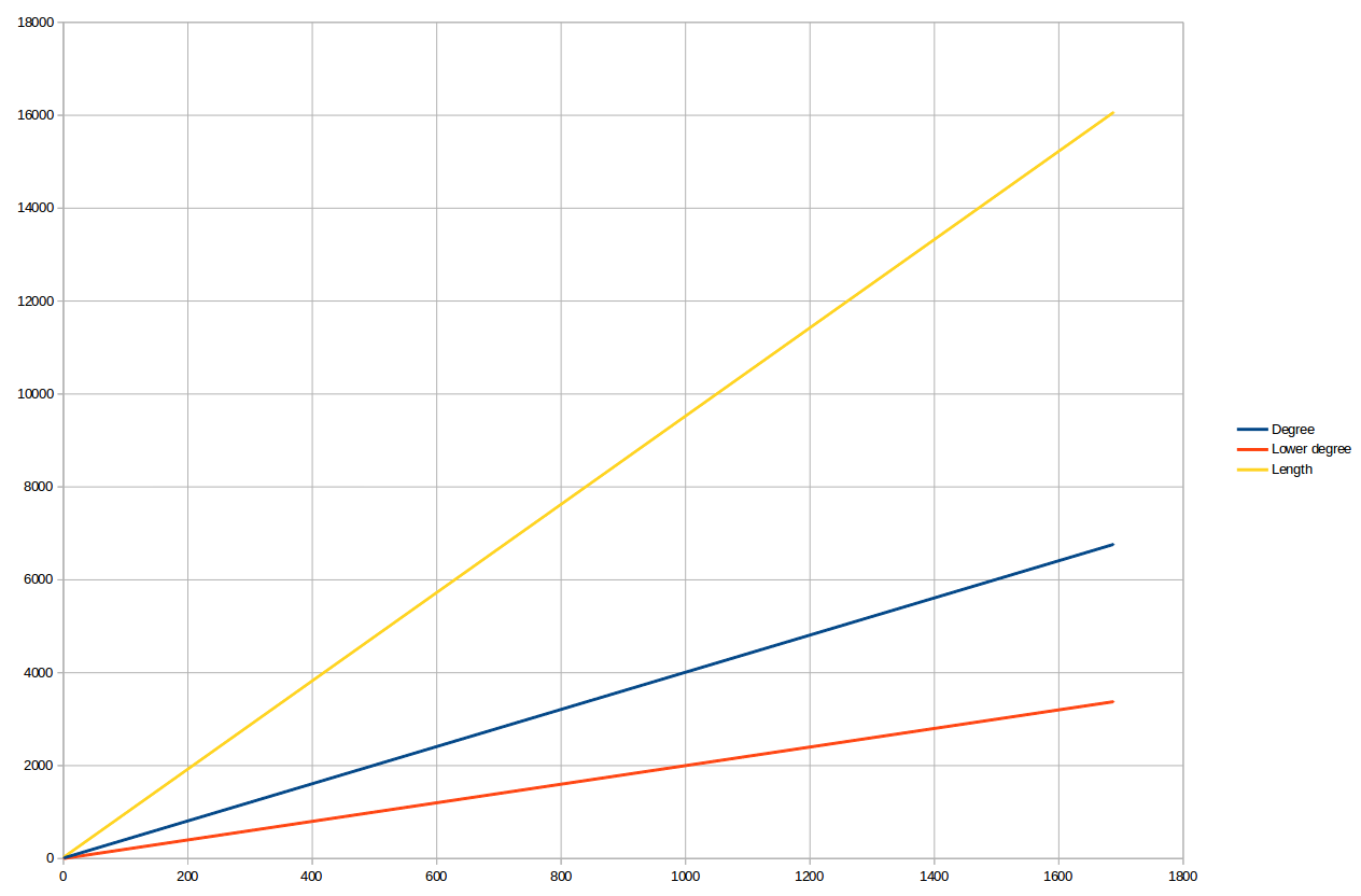
Figure 1: Degrees, lower degrees and lengths of the third coordinate of the sequence produced by algorithm for $F$.

These calculations take 57 minutes and 32 seconds and consume 7GB RAM. According to theorem 1, we need to perform at most 1688 steps of the algorithm in order to find the inverse mapping. It appears that algorithm does not stop in 1688 steps for any coordinate. For the previous examples we presented degrees, lower degrees and lengths of chosen coordinate of polynomial mappings produced by the algorithm in table. In this example due to large size of the numbers we present such a data in figure 1 instead.

Alternatively we can use reductions modulo prime numbers and then obtain $G$ using Chinese Remainder Theorem. For example, after reducing $F$ modulo 2 we obtain $\overline{F}^{2}~{}:~{}\mathbb{F}_{2}\rightarrow\mathbb{F}_{2}$ given by the following formula.

$$\overline{F}^{2}:\left\{\begin{array}[]{ll}\overline{F}^{2}_{1}=&X_{1}\\ \overline{F}^{2}_{2}=&X_{2}+X_{1}^{3}\\ \overline{F}^{2}_{3}=&X_{3}+X_{1}^{13}+X_{1}^{7}+X_{1}^{6}X_{2}+X_{1}^{6}X_{3}+X_{1}^{6}X_{4}+X_{1}^{5}+X_{1}X_{2}^{4}+X_{1}^{4}X_{3}\\ &+X_{1}^{2}X_{2}+X_{1}X_{2}^{2}+X_{2}^{3}+X_{1}X_{2}X_{3}+X_{2}^{2}X_{3}+X_{2}^{2}X_{4}\\ \overline{F}^{2}_{4}=&X_{4}+X_{1}^{13}+X_{1}^{11}+X_{1}^{8}X_{2}+X_{1}^{6}X_{2}+X_{1}^{5}X_{2}^{2}+X_{1}^{6}X_{3}+X_{1}^{6}X_{4}+X_{1}^{4}X_{2}\\ &+X_{1}^{2}X_{2}^{3}+X_{1}X_{2}^{4}+X_{1}^{4}X_{4}+X_{1}X_{2}^{2}+X_{2}^{3}+X_{1}^{2}X_{3}+X_{2}^{2}X_{3}+X_{1}X_{2}X_{4}+X_{2}^{2}X_{4}\end{array}\right..$$

Algorithm allows us to find its inverse $\overline{G}^{2}$.

$$\overline{G}^{2}:\left\{\begin{array}[]{ll}\overline{G}^{2}_{1}=&X_{1}\\ \overline{G}^{2}_{2}=&X_{2}+X_{1}^{3}\\ \overline{G}^{2}_{3}=&X_{3}+X_{1}^{2}X_{2}+X_{1}X_{2}^{2}+X_{2}^{3}+X_{1}X_{2}X_{3}+X_{2}^{2}X_{3}+X_{2}^{2}X_{4}\\ \overline{G}^{2}_{4}=&X_{4}+X_{1}X_{2}^{2}+X_{2}^{3}+X_{1}^{2}X_{3}+X_{2}^{2}X_{3}+X_{1}X_{2}X_{4}+X_{2}^{2}X_{4}\end{array}\right..$$

These calculations take 15 seconds using 0,57 GB RAM. The maximum number of steps given by the theorem 1 is equal to 1099. Algorithm does not stop until then.

We observe that it is enough to consider $S=\{2,3,5,7,11,13,17,19,23,29\}$ to reconstruct $G$. One can check that by computing the composition of $F$ and obtained $G$. Times of execution and consumption of memory are presented in table 5. Degrees, lower degrees and length appearing in the third coordinate of the sequence calculated during execution of algorithm for mapping $\overline{F}^{2}$ are presented in figure 2.

$p$	Time of execution	RAM used
2	15 s	0.57 GB
3	1 s	0.2 GB
5	3 min 5 s	2.96 GB
7	5 min	3.94 GB
11	9 min 21 s	5.58 GB
13	4 min 13 s	1.78 GB
17	9 min 40 s	5.65 GB
19	10 min 32 s	5.63 GB
23	11 min 6 s	6.1 GB
29	12 min 59 s	6.53 GB

Table 5: Execution time and memory consumption.

One can observe that the reduction approach run in sequence can last longer than the direct approach for the mapping $F\in\mathbb{Q}[X]^{4}$. However the memory consumption can be smaller. Hence this method can be used for computer with less amount of memory installed. This observation allows us also to use reduction approach together with parallel computations. In this way the time of inverting $F$ can be significantly reduced.

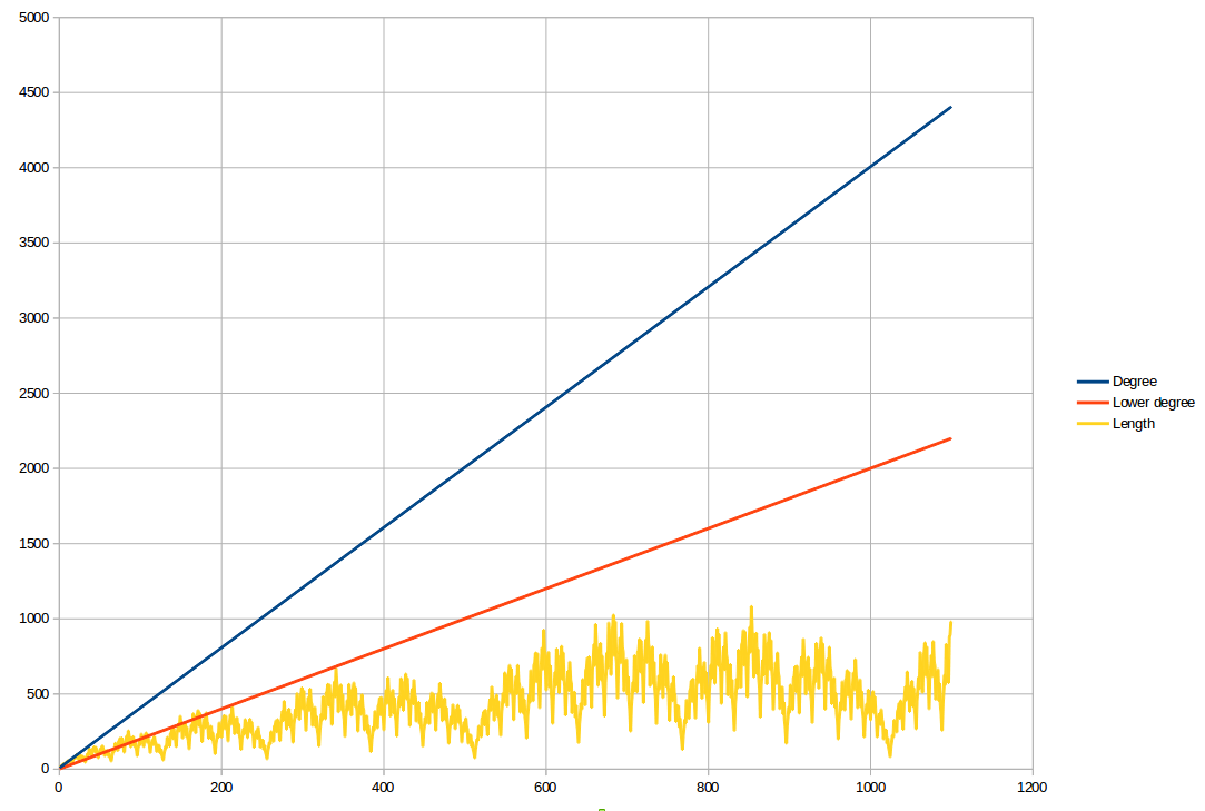
Figure 2: Degrees, lower degrees and lengths of the third coordinate of the sequence produced by algorithm for $\overline{F}^{2}$.

References

- [1] E. Adamus, P. Bogdan, T. Crespo and Z. Hajto, An effective study of polynomial maps, Journal of Algebra and Its Applications, 16 (2017), No.8, 1750141, 13pp
- [2] E. Adamus, P. Bogdan, T. Crespo and Z. Hajto, Pascal finite polynomial automorphisms. Journal of Algebra and Its Applications (2019), 1950124, 10pp, already published on-line
- [3] P. Bogdan, Complexity of the inversion algorithm of polynomial mappings, Schedae Informaticae, 2016, Volume 25, pages 209–225
- [4] L. A. Campbell, Reduction theorems for the Strong Real Jacobian Conjecture, Annales Polonici Mathematici, 110.1 (2014).
- [5] E. Connell, L. van den Dries, Injective polynomial maps and the Jacobian Conjecture, Journal of Pure and Applied Algebra 28 (1983), 235-239
- [6] A. van den Essen, Polynomial automorphisms and the Jacobian Conjecture, Progress in Mathematics 190, Birkhäuser Verlag, 2000.
- [7] J-Ph. Furter, S. Maubach, Locally finite polynomial endomorphisms, Journal of Pure and Applied Algebra 211 (2007) 445–-458.
- [8] K. Ireland, M. Rosen, A Classical Introduction to Modern Number Theory, Springer-Verlag, Graduate Texts in Mathematics, Vol. 84, 1990.
- [9] S. Maubach, Polynomial Automorphisms Over Finite Fields, Serdica Mathematical Journal 27.4 (2001): 343-350
- [10] S. Maubach, R. Willems, Keller Maps of Low Degree over Finite Fields, I. Cheltsov, C. Ciliberto, H. Flenner, J. McKernan, Y. Prokhorov, M. Zaidenberg (eds) Automorphisms in Birational and Affine Geometry, Springer Proceedings in Mathematics and Statistics, vol 79. (2014)