Abstract

We consider distributed optimization where the objective function is spread among different devices, each sending incremental model updates to a central server. To alleviate the communication bottleneck, recent work proposed various schemes to compress (e.g. quantize or sparsify) the gradients, thereby introducing additional variance $\omega\geq 1$ that might slow down convergence. For strongly convex functions with condition number $\kappa$ distributed among $n$ machines, we (i) give a scheme that converges in ${\cal O}((\kappa+\kappa\frac{\omega}{n}+\omega)$ $\log(1/\epsilon))$ steps to a neighborhood of the optimal solution. For objective functions with a finite-sum structure, each worker having less than $m$ components, we (ii) present novel variance reduced schemes that converge in ${\cal O}((\kappa+\kappa\frac{\omega}{n}+\omega+m)\log(1/\epsilon))$ steps to arbitrary accuracy $\epsilon>0$. These are the first methods that achieve linear convergence for arbitrary quantized updates. We also (iii) give analysis for the weakly convex and non-convex cases and (iv) verify in experiments that our novel variance reduced schemes are more efficient than the baselines.

1 Introduction

The training of large scale machine learning models poses many challenges that stem from the mere size of the available training data. The data-parallel paradigm focuses on distributing the data across different compute notes, which operate in parallel on the data. Formally, we consider optimization problems distributed across $n$ nodes of the form

$$\min_{x\in\mathbb{R}^{d}}\left[f(x):=\frac{1}{n}\sum_{i=1}^{n}f_{i}(x)\right]\,,$$ (1)

where $f_{i}\colon\mathbb{R}^{d}\to\mathbb{R}$ for $i=1,\dots,n$ are given as

$$f_{i}(x):={\rm E}_{\zeta\sim{\cal D}_{i}}\left[F(x,\zeta)\right]\,,$$ (2)

with $F\colon\mathbb{R}^{d}\times\Omega\to\mathbb{R}$ being a general loss function. The distributions ${\cal D}_{1},\dots,{\cal D}_{n}$ can be different on every node, which means the functions $f_{1},\dots,f_{n}$ can have completely different minimizers. This frameworks covers stochastic optimization (when either $n=1$ or all ${\cal D}_{i}$ are identical) and empirical risk minimization (for e.g. when the ${\cal D}_{i}$’s are discrete with disjoint support). We denote by $x^{\star}$ an optimal solution of (1), let $f^{\star}\overset{\text{def}}{=}f(x^{\star})$.

1.1 Quantization to Reduce Communication

In typical computing architectures, communication is much slower than computation and the communication bottleneck between workers is a major limiting factor for many large scale applications (such as e.g. deep neural network training), as reported in e.g. Seide et al. (2014); Alistarh et al. (2017); Zhang et al. (2017); Lin et al. (2018). A possible remedy to tackle this issue are for instance approaches that focus on increasing the computation to communication ratio, such as increased mini-batch sizes Goyal et al. (2017), defining local problems for each worker Shamir et al. (2014); Reddi et al. (2016) or reducing the communication frequency McDonald et al. (2009); Zinkevich et al. (2010); You et al. (2017); Stich (2018).

A direction orthogonal to these approaches tries to reduce the size of the messages—typically gradient vectors—that are exchanged between the nodes Seide et al. (2014); Strom (2015); Alistarh et al. (2017); Wen et al. (2017); Grishchenko et al. (2018). These quantization techniques rely on (lossy) compression of the gradient vectors. In the simplest form, these schemes limit the number of bits that are used to represent floating point numbers Gupta et al. (2015); Na et al. (2017), reducing the size of a $d$-dimensional (gradient) vector by a constant factor. Random dithering approaches attain up to ${\cal O}(\sqrt{d})$ compression Seide et al. (2014); Alistarh et al. (2017); Wen et al. (2017). The most aggressive schemes reach ${\cal O}(d)$ compression by only sending a constant number of bits per iteration Suresh et al. (2017); Konečný & Richtárik (2016); Alistarh et al. (2018); Stich et al. (2018). An alternative approach is not to compute the gradient and subsequently compress it, but to update a subset of elements of the iterate $x$ using coordinate descent type updates Richtárik & Takáč (2016); Fercoq et al. (2014); Mishchenko et al. (2019).

Recently, Mishchenko et al. (2018) proposed the first method that successfully applies the gradient quantization technique to the distributed optimization problem (1) with a non-smooth regularizer.

1.2 Contributions

We now briefly outline the key contributions of our work:

General compression. We generalize the method presented in Mishchenko et al. (2018) allowing for arbitrary compression (e.g., quantization and sparsification) operators. Our analysis is tight, i.e. we recover their convergence rates as a special case. Our more general approach allows to choose freely the compression operators that perform best on the available system resources and can thus offer gains in training time over the previous method that is tied to a single class of operators.

Variance reduction. We present several variance reduced extensions of our methods for distributed training. In particular, and in contrast to Mishchenko et al. (2018), our methods converge to the optimum and not merely to a neighborhood, without any loss in convergence rate. The quantized SVRG method of Alistarh et al. (2017) did not only rely on a specific compression scheme, but also on exact communication from time to time (epoch gradients), both restrictions been overcome here.

Convex and non-convex problems. We provide concise convergence analysis for our novel schemes for the strongly-convex, the (weakly) convex and non-convex setting. Our analysis recovers the respective rates of earlier schemes without communication compression and shows that compression can provide huge benefits when communication is a bottleneck.

Experiments. We compare the novel variance reduced schemes with various baselines. In the experiments we leverage the flexibility of our approach—allowing to freely chose a quantization scheme with optimal parameters—and demonstrate on par performance with the baselines in terms of iterations, but considerable savings in terms of total communication cost.

2 Related Work

Gradient compression schemes have successfully been used in many implementations as a heuristic to reduce communication cost, such as for instance in 1BitSGD Seide et al. (2014); Strom (2015) that rounds the gradient components to either -1 or 1, and error feedback schemes aim at reducing quantization errors among iterations, for instance as in Lin et al. (2018). In the discussion below we focus in particular on schemes that enjoy theoretical convergence guarantees.

2.1 Quantization and Sparsification

A class of very common quantization operators is based on random dithering Goodall (1951); Roberts (1962) and can be described as the random operators $Q\colon\mathbb{R}^{d}\to\mathbb{R}^{d}$,

$$Q(x)=\operatorname{sign}(x)\cdot\lVert x\rVert_{p}\cdot\frac{1}{s}\cdot\left\lfloor s\frac{\lvert x\rvert}{\lVert x\rVert_{p}}+\xi\right\rfloor$$ (3)

for random variable $\xi\sim_{\rm u.a.r.}[0,1]^{d}$, parameter $p\geq 1$, and $s\in\mathbb{N}_{+}$, denoting the levels of the rounding. Its unbiasedness property, ${\rm E}_{\xi}\left[Q(x)\right]=x$, $\forall x\in\mathbb{R}^{d}$, is the main catalyst of the theoretical analyses. The quantization (3) was for instance used in QSGD for $p=2$ Alistarh et al. (2017), in TernGrad for $s=1$ and $p=\infty$ Wen et al. (2017) or for general $p\geq 1$ and $s=1$ in DIANA Mishchenko et al. (2018). For $p=2$ the expected sparsity is ${\rm E}_{\xi}\left[\lVert Q(x)\rVert_{0}\right]={\cal O}(s(s+\sqrt{d}))$ Alistarh et al. (2017) and encoding a nonzero coordinate of $Q(x)$ requires ${\cal O}(\log(s))$ bits.

Much sparser vectors can be obtained by random sparsification techniques that randomly mask the input vectors and only preserve a constant number of coordinates Suresh et al. (2017); Konečný & Richtárik (2016); Wangni et al. (2018); Stich et al. (2018). Experimentally is has been shown that deterministic masking—for instance selecting the largest components in absolute value Dryden et al. (2016); Aji & Heafield (2017)—can outperform the random techniques. However, as these schemes are biased, they resisted careful analysis until very recently Alistarh et al. (2018); Stich et al. (2018). We will not further distinguish between sparsification and quantization approaches, and refer to both of these compression schemes them as ‘quantization’ in the following.

Also schemes with error compensation techniques have recently been successfully vanquished, for instance for unbiased quantization on quadratic functions Wu et al. (2018) and for unbiased and biased quantization on strongly convex functions Stich et al. (2018). These schemes suffer much less from large quantization errors, and can tolerate higher variance (both in practice an theory) than the methods above without error compensation.

2.2 Quantization in Distributed Learning

In centralized approaches, all nodes communicate with a central node (parameter sever) that coordinates the optimization process. An algorithm of specific interest to solve problem (1) is mini-batch SGD Dekel et al. (2012); Takáč et al. (2013), a parallel version of stochastic gradient descent (SGD) Robbins & Monro (1951); Nemirovski et al. (2009). In mini-batch SGD, full gradient vectors have to be communicated to the central node and hence it is natural to incorporate gradient compression to reduce the cost of the communication rounds. Khirirat et al. (2018) study quantization in the deterministic setting, i.e. when the gradients $\nabla f_{i}(x)$ can be computed without noise, and show that parallel gradient descent with unbiased quantization converges to a neighborhood of the optimal solution on strongly convex functions. Mishchenko et al. (2018) consider the stochastic setting as in (1) and show convergence of SGD with unbiased quantization to a neighborhood of a stationary point for non-convex and strongly convex functions; the analysis in Wu et al. (2018) only applies to quadratic functions. The method of Stich et al. (2018) can also be parallelized as shown by Cordonnier (2018) and converges to the exact solution on strongly convex functions.

Decentralized methods do not require communication with a centralized node. Tang et al. (2018) consider unbiased quantization and show convergence to the neighborhood of a stationary point on non-convex functions under very rigid assumptions on the quantization, i.e. allowing only ${\cal O}(1)$ compression, Koloskova et al. (2019) relax those constraints but only consider strongly convex functions.

2.3 Quantization and Variance Reduction

Variance reduced methods Roux et al. (2012); Johnson & Zhang (2013); Shalev-Shwartz & Zhang (2013); Defazio et al. (2014); Qu et al. (2015); Shalev-Shwartz (2016); Qu et al. (2016); Csiba & Richtárik (2015); Csiba et al. (2015); Nguyen et al. (2017); Gower et al. (2018); Zhou (2018) admit linear convergence on empirical risk minimization problems, surpassing the rate of vanilla SGD Bottou (2010). Alistarh et al. (2017) proposed a quantized version of SVRG Johnson & Zhang (2013), but the proposed scheme relies on broadcasting exact (unbiased) gradients every epoch. This restriction has been overcome in Künstner (2017) but only for high-precision quantization. Here we alleviate these restrictions and present quantization not only for SVRG but also for SAGA Defazio et al. (2014). Our analysis also supports a version of SVRG whose epoch lengths are not fixed, but random, similar as e.g. in Lei & Jordan (2017); Hannah et al. (2018). Our base version (denoted as L-SVRG) is slightly different and inspired by observations made in Hofmann et al. (2015); Raj & Stich (2018) and following closely Kovalev et al. (2019).

2.4 Orthogonal Approaches

There are other approaches aiming to reduce the communication cost, such as increased mini-batch sizes Goyal et al. (2017), defining local problems for each worker Shamir et al. (2014); Jaggi et al. (2014); Ma et al. (2015); Reddi et al. (2016); Ma et al. (2017), reducing the communication frequency McDonald et al. (2009); Zinkevich et al. (2010); You et al. (2017); Stich (2018) or distributing along features Richtárik & Takáč (2016); Fercoq et al. (2014). However, we are not considering such approaches here.

3 General Definitions

Definition 1 ($\mu$-strong convexity).

A differentiable function $f\colon\mathbb{R}^{d}\to\mathbb{R}$ is $\mu$-strongly convex for $\mu>0$, if for all $x,y\in\mathbb{R}^{d}$

$$f(y)\geq f(x)+\left\langle\nabla f(x),y-x\right\rangle+\frac{\mu}{2}\lVert x-y\rVert_{2}^{2}\,.$$ (4)

Definition 2 ($L$-smoothness).

A differentiable function $f\colon\mathbb{R}^{d}\to\mathbb{R}$ is $L$-smooth for $L>0$, if for all $x,y\in\mathbb{R}^{d}$

$$f(y)\leq f(x)+\left\langle\nabla f(x),y-x\right\rangle+\frac{L}{2}\lVert x-y\rVert_{2}^{2}\,.$$ (5)

Definition 3.

The prox operator $\operatorname{prox}_{\gamma R}\colon\mathbb{R}^{d}\to\mathbb{R}^{d}$ is defined as

$$\operatorname{prox}_{\gamma R}(x)=\operatorname{argmin}_{y\in\mathbb{R}^{d}}\left\{\gamma R(y)+\frac{1}{2}\lVert y-x\rVert_{2}^{2}\right\}\,,$$

for $\gamma>0$ and a closed convex regularizer $R\colon\mathbb{R}^{d}\to\mathbb{R}\cup\{\infty\}$.

4 Quantization Operators

Our analysis depends on a general notion of quantization operators with bounded variance.

Definition 4 ($\omega$-quantization).

A random operator $Q\colon\mathbb{R}^{d}\to\mathbb{R}^{d}$ with the properties

$${\rm E}_{Q}\left[Q(x)\right]=x\,, {\rm E}_{Q}\left[\lVert Q(x)\rVert_{2}^{2}\right]\leq(\omega+1)\lVert x\rVert_{2}^{2}\,,$$ (6)

for all $x\in\mathbb{R}^{d}$ is a $\omega$-quantization operator. Here ${\rm E}_{Q}\left[\cdot\right]$ denotes the expectation over the (internal) randomness of $Q$.

Remark 1.

As ${\rm E}\left[\lVert X-{\rm E}\left[X\right]\rVert_{2}^{2}\right]={\rm E}\left[\lVert X\rVert_{2}^{2}\right]-\lVert{\rm E}\left[X\right]\rVert_{2}^{2}$ for any random vector $X$, equation (6) implies

$${\rm E}_{Q}\left[\lVert Q(x)-x\rVert_{2}^{2}\right]\leq\omega\lVert x\rVert_{2}^{2}\,.$$ (7)

For instance, we see that $\omega=0$ implies $Q(x)=x$.

Remark 2.

Besides the variance bound, Definition 4 does not impose any further restrictions on $Q(x)$. However, for all applications it is advisable to consider operators $Q$ that achieve a considerable compression, i.e. $Q(x)$ should be cheaper to encode than $x$.

We will now give examples of a few $\omega$-quantization operators that also achieve compression, either by quantization techniques, or by enforcing sparsity (cf. Sec. 2.1).

Example 1 (random dithering).

The operator given in (3) satisfies (6) for $\omega(x):=2+\frac{\lVert x\rVert_{1}\lVert x\rVert_{p}}{s\lVert x\rVert_{2}^{2}}$ for every fixed $x\in\mathbb{R}^{d}$, and $\omega(x)$ is a function monotonically decreasing in $p$. Moreover,

$$\omega={\cal O}\left(\frac{d^{1/p}+d^{1/2}}{s}\right)$$

for $p\geq 1$, $s\geq 1$ and all $x\in\mathbb{R}^{d}$.

For $p=2$ this bound was proven by Alistarh et al. (2017). Here we generalize the analysis to arbitrary $p\geq 1$.

Proof.

In view of (3) we have

$${\rm E}_{Q}\left[\lVert Q(x)\rVert_{2}^{2}\right]=\frac{\lVert x\rVert_{p}^{2}}{s^{2}}\sum_{i=1}^{d}\left(\underbrace{\ell_{i}^{2}(1-p_{i})+(\ell_{i}+1)^{2}p_{i}}_{\leq\ell_{i}^{2}+(2\ell_{i}+1)p_{i}}\right)$$

for integers $\ell_{i}\leq s\lvert x_{i}\rvert/\lVert x\rVert_{p}\leq\ell_{i}+1$ and probabilities $p_{i}=s\lvert x_{i}\rvert/\lVert x\rVert_{p}-\ell_{i}\leq s\lvert x_{i}\rvert/\lVert x\rVert_{p}$. Therefore,

$${\rm E}_{Q}\left[\lVert Q(x)\rVert_{2}^{2}\right] \leq\frac{\lVert x\rVert_{p}^{2}}{s^{2}}\sum_{i=1}^{d}\left(\ell_{i}^{2}+(2\ell_{i}+1)\frac{s\lvert x_{i}\rvert}{\lVert x\rVert_{p}}\right)$$

$$\leq\frac{\lVert x\rVert_{p}^{2}}{s^{2}}\left(s^{2}\frac{\lVert x\rVert_{2}^{2}}{\lVert x\rVert_{p}^{2}}+2s^{2}\frac{\lVert x\rVert_{2}^{2}}{\lVert x\rVert_{p}^{2}}+s\frac{\lVert x\rVert_{1}}{\lVert x\rVert_{p}}\right)$$

as $\ell_{i}\leq s\lvert x_{i}\rvert/\lVert x\rVert_{p}$. This proves the bound on $\omega(w)$. By Hölder’s inequality $\lVert x\rVert_{1}\leq d^{1/2}\lVert x\rVert_{2}$ and $\lVert x\rVert_{p}\leq d^{1/p-1/2}\lVert x\rVert_{2}$ for $1\leq p\leq 2$ and for $p\geq 2$ the inequality $\lVert x\rVert_{p}\leq\lVert x\rVert_{2}$ imply the upper bound on $\omega$ for all $x\in\mathbb{R}^{d}$. ∎

Example 2 (random sparsifiction).

The random sparsification operator $Q(x)=\frac{d}{r}\cdot\xi\otimes x$ for random variable $\xi\sim_{\rm u.a.r.}\{y\in\{0,1\}^{d}\colon\lVert y\rVert_{0}=r\}$ and sparsity parameter $r\in\mathbb{N}_{+}$ is a $\omega=\frac{d}{r}-1$ quantization operator.

For a proof see e.g. (Stich et al., 2018, Lemma A.1).

Example 3 (block quantization).

The vector $x\in\mathbb{R}^{d}$ is first split into $t$ blocks and then each block $v_{i}$ is quantized using random dithering with $p=2$, $s=1$. If every block has the same size $d/t$, then this gives a quantization operator with $\omega=\sqrt{d/t}+1$, otherwise $\omega=\max_{i\in[t]}\sqrt{|v_{i}|}+1$.

Block quantization was e.g. used in Alistarh et al. (2017) and is also implemented (in a similar fashion) in the CNTK toolkit Seide & Agarwal (2016). The proofs of the claimed bounds can be found in Mishchenko et al. (2018).

5 DIANA with Arbitrary Quantization

We are now ready to present the first algorithm and its theoretical properties. In this section we consider the regularized problem (1):

$$\min_{x\in\mathbb{R}^{d}}\left[f(x)+R(x):=\frac{1}{n}\sum_{i=1}^{n}f_{i}(x)+R(x)\right]\,,$$ (8)

where $R\colon\mathbb{R}^{d}\to\mathbb{R}\cup\{+\infty\}$ denotes a closed convex regularizer.

5.1 DIANA

Algorithm 1 is identical to the DIANA algorithm in Mishchenko et al. (2018). However, we allow for arbitrary $\omega$-quantization operators, whereas Mishchenko et al. (2018) consider random dithering quantization operators (3) with $p\geq 1$ and $s=1$ only.

In Algorithm 1, each worker $i=1,\dots,n$ queries the oracle and computes an unbiased stochastic gradient $g_{i}^{k}$ in iteration $k$, i.e. ${\rm E}\left[g_{i}^{k}\mid x^{k}\right]=\nabla f_{i}(x^{k})$. A naïve approach would be to directly send the quantized gradients, $Q(g_{i}^{k})$, to the master node. However, this simple scheme does not only introduce a lot of noise (for instance, even at the optimal solution $x^{\star}\in\mathbb{R}^{d}$ the norms of the stochastic gradients do not vanish), but also does in general not converge for nontrivial regularizers $R\not\equiv 0$. Instead, in Algorithm 1 each worker maintains a state $h_{i}^{k}\in\mathbb{R}^{d}$ and quantizes only the difference $g_{i}^{k}-h_{i}^{k}$ instead. If (and this we show below) $h_{i}^{k}$ converges to $\nabla f_{i}(x^{\star})$ for ($k\to\infty$), the variance of the quantization can be massively reduced compared to the naïve scheme. Both the worker and the master node update $h_{i}^{k}$ based on the transmitted (quantized) vector $\hat{\Delta}_{i}^{k}\in\mathbb{R}^{d}$. Note that the quantization operator $Q$ should be chosen so that the transmission of $\hat{\Delta}_{i}^{k}$ requires significantly less bits than the transmission of the full $d$-dimensional vector.

5.2 Convergence of Algorithm 1

We make the following technical assumptions:

Assumption 1.

In problem (8) we assume each $f_{i}\colon\mathbb{R}^{d}\to\mathbb{R}$ to be $\mu$-strongly convex and $L$-smooth. We assume that each $g_{i}^{k}$ in Algorithm 1 has bounded variance

$${\rm E}\left[\lVert g_{i}^{k}-\nabla f_{i}(x^{k})\rVert_{2}^{2}\right] \leq\sigma_{i}^{2}\,, \forall k\geq 0,i=1,\dots,n$$ (9)

for constants $\sigma_{i}\leq\infty$, $\sigma^{2}:=\frac{1}{n}\sum_{i=1}^{n}\sigma_{i}^{2}$.

Input: learning rates $\alpha>0$, and $\gamma>0$, initial vectors $x^{0}$, $h_{1}^{0},\dots,h_{n}^{0}$ and $h^{0}=\frac{1}{n}\sum_{i=1}^{n}h_{i}^{0}$

1 for $k=0,1,\dots$ do

2       broadcast $x^{k}$ to all workers

3       for  $i=1,\dots,n$  do in parallel $\triangleright$ worker side

4             sample $g_{i}^{k}$ such that ${\rm E}\left[g_{i}^{k}\mid x^{k}\right]=\nabla f_{i}(x^{k})$

5             $\Delta_{i}^{k}=g_{i}^{k}-h_{i}^{k}$

6             $\hat{\Delta}_{i}^{k}=Q(\Delta_{i}^{k})$

7             $h_{i}^{k+1}=h_{i}^{k}+\alpha\hat{\Delta}_{i}^{k}$

8             $\hat{g}_{i}^{k}=h_{i}^{k}+\hat{\Delta}_{i}^{k}$

9            

10       end for

      $q^{k}=\tfrac{1}{n}\sum_{i=1}^{n}\hat{\Delta}_{i}^{k}$

        $\triangleright$ gather quantized updates

11       $\hat{g}^{k}=\tfrac{1}{n}\sum_{i=1}^{n}\hat{g}_{i}^{k}$

12       $x^{k+1}=\operatorname{prox}_{\gamma R}(x^{k}-\gamma\hat{g}^{k})$

13       $h^{k+1}=\tfrac{1}{n}\sum_{i=1}^{n}h_{i}^{k+1}$

14 end for

Algorithm 1 DIANA with arbitrary unbiased quantization

The main theorem of this section, presented next, establishes linear convergence of Algorithm 1 with arbitrary $\omega$-quantization schemes.

Theorem 1.

Consider Algorithm 1 with $\omega$-quantization $Q$ and stepsize $\alpha\leq\frac{1}{\omega+1}$. Define the Lyapunov function

$$\Psi^{k}:=\lVert x^{k}-x^{\star}\rVert_{2}^{2}+\frac{c\gamma^{2}}{n}\sum_{i=1}^{n}\lVert h_{i}^{k}-\nabla f_{i}(x^{\star})\rVert_{2}^{2}$$

for $c\geq\frac{4\omega}{\alpha n}$ and assume $\gamma\leq\frac{2}{(\mu+L)(1+\frac{2\omega}{n}+c\alpha)}$ and $\gamma\leq\frac{\alpha}{2\mu}$. Then under Assumption 1:

$${\rm E}\left[\Psi^{k}\right]\leq(1-\gamma\mu)^{k}\Psi^{0}+\frac{2}{\mu(\mu+L)}\sigma^{2}\,.$$ (10)

Corollary 1.

Let $c=\frac{4\omega}{\alpha n}$, $\alpha=\frac{1}{\omega+1}$ and $\gamma=\min\left\{\frac{2}{(\mu+L)(1+\frac{6\omega}{n})},\frac{1}{2\mu(\omega+1)}\right\}$. Furthermore, define $\kappa=\frac{L+\mu}{2\mu}$. Then the conditions of Theorem 1 are satisfied and the leading term in the iteration complexity bound is

$$\frac{1}{\gamma\mu}=\kappa+\kappa\frac{2\omega}{n}+2(\omega+1)\,.$$

Remark 3.

For the special case of quantization (3) in arbitrary $p$-norms and $s=1$, this result recovers Mishchenko et al. (2018) up to small differences in the constants.

6 Variance Reduction for Quantized Updates

Input: learning rates $\alpha>0$ and $\gamma>0$, initial vectors $x^{0},h_{1}^{0},\dots,h_{n}^{0}$, $h^{0}=\frac{1}{n}\sum_{i=1}^{n}h_{i}^{0}$

1 for $k=0,1,\ldots$ do

       sample random

        $\triangleright$ only for Variant 1

2       $u^{k}=\begin{cases}1,&\text{with probability }\frac{1}{m}\\ 0,&\text{with probability }1-\frac{1}{m}\\ \end{cases}$

3       broadcast $x^{k}$, $u^{k}$ to all workers

4       for $i=1,\ldots,n$ do in parallel $\triangleright$ worker side

5             pick random $j_{i}^{k}\sim_{\rm u.a.r.}[m]$

6             $\mu_{i}^{k}=\frac{1}{m}\sum\limits_{j=1}^{m}\nabla f_{ij}(w_{ij}^{k})$

7             $g_{i}^{k}=\nabla f_{ij_{i}^{k}}(x^{k})-\nabla f_{ij_{i}^{k}}(w_{ij_{i}^{k}}^{k})+\mu_{i}^{k}$

8             $\hat{\Delta}_{i}^{k}=Q(g_{i}^{k}-h_{i}^{k})$

9             $h_{i}^{k+1}=h_{i}^{k}+\alpha\hat{\Delta}_{i}^{k}$

10             for $j=1,\ldots,m$ do

                  

                   $\triangleright$ Variant 1 (L-SVRG): update epoch gradient if $u^{k}=1$

11                   $w_{ij}^{k+1}=\begin{cases}x^{k},&\text{if }u^{k}=1\\ w_{ij}^{k},&\text{if }u^{k}=0\\ \end{cases}$

                  

                   $\triangleright$ Variant 2 (SAGA): update gradient table

12                   $w_{ij}^{k+1}=\begin{cases}x^{k},&j=j_{i}^{k}\\ w_{ij}^{k},&j\neq j_{i}^{k}\\ \end{cases}$

13             end for

14            

15       end for

      $h^{k+1}\!=\!h^{k}\!+\!\frac{\alpha}{n}\displaystyle\sum_{i=1}^{n}\hat{\Delta}_{i}^{k}$

        $\triangleright$ gather quantized updates

16       $g^{k}=\frac{1}{n}\sum\limits_{i=1}^{n}(\hat{\Delta}_{i}^{k}+h_{i}^{k})$

17       $x^{k+1}=x^{k}-\gamma g^{k}$

18      

19 end for

Algorithm 2 VR-DIANA based on L-SVRG (Variant 1), SAGA (Variant 2)

We now move to the main contribution of this paper and present variance reduced methods with quantized gradient updates. In this section we assume that each component $f_{i}$ of $f$ in (1) has finite-sum structure:

$$f_{i}(x)=\frac{1}{m}\sum\limits_{j=1}^{m}f_{ij}(x)\,,$$ (11)

The assumption that the number of components $m$ is the same for all functions $f_{i}$ is made for simplicity only. As can seen from (10), one of the main disadvantages of Algorithm 1 is the fact that we can only guarantee linear convergence to a $\frac{2}{\mu(\mu+L)}\frac{\sigma^{2}}{n}$-neighborhood of the optimal solution. In particular, the size of the neighborhood depends on the size of $\sigma^{2}$, which measures the average variance of the stochastic gradients $g_{i}^{k}$ across the workers $i\in[n]$. In contrast, variance reduced methods converge linearly for arbitrary accuracy $\epsilon>0$.

6.1 The main challenge

Let us recall that the variance reduced method SVRG Johnson & Zhang (2013) computes the full gradient $\nabla f(x)$ in every epoch. To achieve this in the distributed setting (1), each worker $i$ must compute the gradient $\nabla f_{i}(x)$ and send this vector (exactly) either to the master node or broadcast it to all other workers. It might be tempting to replace this expensive communication step with quantized gradients instead, i.e. to rely on the aggregate $y_{Q}:=\frac{1}{n}\sum_{i=1}^{n}Q(\nabla f_{i}(x))$ instead. However, the error $\lVert y_{Q}-\nabla f(x)\rVert$ can be arbitrarily large (e.g. it will even not vanish for $x=x^{\star}$) and this simple scheme does not achieve variance reduction (cf. also the discussion in Künstner (2017)). Our approach to tackle this problem is via the quantization of gradient differences. Similarly to the previous section, we propose that each worker maintains a state $h_{i}^{k}\in\mathbb{R}^{d}$, and only quantizes gradient differences; for instance update $h_{i}^{k+1}=h_{i}^{k}+Q(h_{i}^{k}-\nabla f_{i}(x))$ (we assume this for ease of exposition, the actual scheme is slightly different). We can now set $h^{k}=\frac{1}{n}\sum_{i=1}^{n}h_{i}^{k}$, which turns out to be a much more robust estimator of $\nabla f(x)$. By means of proving that $\lVert h_{i}^{k}-\nabla f_{i}(x^{\star})\rVert\to 0$ for $(k\to\infty)$ we are able to derive the first variance reduced method that only exchanges quantized gradient updates among workers.

6.2 Three new algorithms

We propose in total three variance reduced algorithms, which are derived from either SAGA (displayed in Algorithm 2, Variant 2), SVRG (Algorithm 3 provided in the appendix) and L-SVRG (Algorithm 2, Variant 1), a variant of SVRG with random epoch length and described in Kovalev et al. (2019). We prove global linear convergence in the strongly convex case and ${\cal O}(1/k)$ convergence in convex and non-convex cases. Moreover, our analysis is very general in the sense that the original complexity results for all three algorithms can be obtained by setting $\omega=1$ (no quantization).

Comments on Algorithm 2. In analogy to Algorithm 1, each node maintains a state $h_{i}^{k}\in\mathbb{R}^{d}$ that aims to reduce the variance introduced by the quantized communication. In contrast to the variance reduced method in Alistarh et al. (2017) that required the communication of the uncompressed gradients for every iteration of the inner loop (SVRG based scheme), here we communicate only quantized vectors.

Each worker $i=1,\dots,n$ computes its stochastic gradient $g_{i}^{k}$ in iteration $k$ by the formula given by the specific variance reduction type (SVRG, SAGA, L-SVRG), such that ${\rm E}\left[g_{i}^{k}\mid x^{k}\right]=\nabla f_{i}(x^{k})$. Subsequently, the DIANA scheme is applied. Each worker in Algorithms 2 and 3 maintains a state $h_{i}^{k}\in\mathbb{R}^{d}$ and quantizes only the difference $g_{i}^{k}-h_{i}^{k}$. This quantized vector $\hat{\Delta}_{i}^{k}$ is then sent to the master node which in turn updates its local copy of $h_{i}^{k}$. Thus both the $i$-th worker and the master node have access to $h_{i}^{k}$ even though it has never been transmitted in full (but instead incrementally constructed from the $\hat{\Delta}_{i}^{k}$’s).

The algorithm based on SAGA maintains on each worker a table of gradients, $\nabla f_{ij}(w_{ij}^{k})$ (so the computation of $\mu_{i}^{k}$ on line 2 can efficiently be implemented). The algorithms based on SAGA just need to store the epoch gradients $\frac{1}{m}\sum_{i=1}^{n}\nabla f_{ij}(w_{i}j^{k})$ that needs only to be recomputed whenever the $w_{ij}^{k}$’s change. Which is either after a fixed number of steps in SVRG, or after a random number of steps as in L-SVRG. These aspects of the algorithm are not specific to quantization and we refer the readers to e.g. Raj & Stich (2018) for a more detailed exposition.

Algorithm	$\omega$	Convergence rate	Convergence rate	Communication
		strongly convex	non-convex	cost per iter.
VR without	$1$	$\hat{{\cal O}}\left(\kappa+m\right)$	${\cal O}\left(\frac{m^{2/3}}{\varepsilon}\right)$	${\cal O}(dn)$
quantization
VR with random	$\sqrt{d}$	$\hat{{\cal O}}\left(\kappa+\kappa\frac{\sqrt{d}}{n}+m+\sqrt{d}\right)$	${\cal O}\left(\left(\frac{\sqrt{d}}{n}\right)^{1/2}\frac{m^{2/3}}{\epsilon}\right)$	${\cal O}(n\sqrt{d})$
dithering ($p=2,s=1$)
VR with random	$\frac{d}{r}$	$\hat{{\cal O}}\left(\kappa+\kappa\frac{d}{n}+m+d\right)$	${\cal O}\left(\frac{d}{\sqrt{n}}\frac{m^{2/3}}{\epsilon}\right)$	${\cal O}(n)$
sparsification ($r=\text{const}$)
VR with	$n$	$\hat{{\cal O}}\left(\kappa+m+n\right)$	${\cal O}\left(\frac{m^{2/3}}{\epsilon}\right)$	${\cal O}(n^{2})$
block quantization ($t=d/n^{2}$)

Table 1: This table compares variance reduced methods with different levels of quantization. The $\hat{{\cal O}}$ notation omits $\log 1/\varepsilon$ factors and we assume $\omega\leq m$ ($\omega\leq m^{2/3}$ for non-convex case) for ease of presentation. For block quantization (last row), the convergence rate is identical to the method without quantization (first row) but the savings in communication is at least $d/n$, assuming $d\geq n$. (in number of total coordinates, here we did for simplicity not consider further savings that the random dithering approach offers in terms of less bits per coordinate). This table shows that quantization is meaningful and can provide huge benefits, especially when communication is a bottleneck.

7 Convergence of VR-DIANA (Algorithm 2)

We make the following technical assumptions (out of which only the first one is shared among all theorems in this section):

Assumption 2.

In problem (1) assume the finite-sum structure (11) for each $f_{i}$. Further assume each function $f_{ij}\colon\mathbb{R}^{d}\to\mathbb{R}$ to be $L$-smooth.

Assumption 3.

Assume each function $f_{i}\colon\mathbb{R}^{d}\to\mathbb{R}$ to be $\mu$-strongly convex, $\mu>0$ and each $f_{ij}\colon\mathbb{R}^{d}\to\mathbb{R}$ to be convex.

Assumption 4.

Assume each function $f_{ij}\colon\mathbb{R}^{d}\to\mathbb{R}$ to be convex.

We are now ready to proceed with the main theorems.

7.1 Strongly convex case

Theorem 2 (Strongly convex case).

Consider Algorithm 2 with $\omega$-quantization $Q$, and step size $\alpha\leq\frac{1}{\omega+1}$. For $b=\frac{4(\omega+1)}{\alpha n^{2}}$, $c=\frac{16(\omega+1)}{\alpha n^{2}}$, $\gamma=\frac{1}{L\left(1+36(\omega+1)/n\right)}$, define the Lyapunov function

$$\psi^{k}=\lVert x^{k}-x^{\star}\rVert_{2}^{2}+b\gamma^{2}H^{k}+c\gamma^{2}D^{k}\,,$$

where

$$H^{k}=\sum\limits_{i=1}^{n}\lVert h_{i}^{k}-\nabla f_{i}(x^{\star})\rVert_{2}^{2}\,,$$

and

$$D^{k}=\sum\limits_{i=1}^{n}\sum\limits_{j=1}^{m}\lVert\nabla f_{ij}(w_{ij}^{k})-\nabla f_{ij}(x^{\star})\rVert_{2}^{2}\,.$$

Then under Assumption 2 and 3

$${\rm E}\left[\psi^{k+1}\right]\leq(1-\rho)\psi^{k},$$

where $\rho\overset{\text{def}}{=}\min\left\{\frac{\mu}{L\left(1+36\frac{\omega+1}{n}\right)},\frac{\alpha}{2},\frac{3}{8m}\right\}$ and the expectation is conditioned on the previous iterate.

Corollary 2.

Let $\alpha=\frac{1}{\omega+1}$. To achieve precision ${\rm E}\left[\|x^{k}-x^{\star}\|_{2}^{2}\right]\leq\varepsilon\psi^{0}$ VR-DIANA needs ${\cal O}\left((\kappa+\kappa\frac{\omega}{n}+m+\omega)\log\frac{1}{\epsilon}\right)$ iterations.

Remark 4.

We would like to mention that even we do not consider the regularized problem in the second part, using our analysis, one can easily extend our result to non-smooth regularizer just by exploiting non-expansiveness of the proximal operator.

Recall that variance reduced methods (such as SAGA or SVRG) converge at rate $\hat{{\cal O}}(\kappa+m)$ in this setting (cf. Table 1). The additional variance of the quantization operator enters the convergence rate in two ways: firstly, (i), as an additive component. However, in large scale machine learning applications the number of data samples $m$ on each machine is expected to be huge. Thus this additive component affects the rate only mildly. Secondly, (ii), and more severely, as a multiplicative component $\frac{\kappa\omega}{n}$. However, we see that this factor is discounted by $n$, the number of workers. Thus by choosing a quantization operator with $\omega={\cal O}(n)$, this term can be controlled. In summary, by choosing a quantization operator with $\omega={\cal O}(\min\{n,m\})$, the rate of VR-DIANA becomes identical to the convergence rate of the vanilla variance reduced schemes without quantization. This shows the importance of algorithms that support arbitrary quantization schemes and that do not depend on a specific quantization scheme.

7.2 Convex case

Let us now look at the convergence under (standard) convexity assumption, that is, $\mu=0$. Then by taking output to be some iterate $x^{k}$ with uniform probability instead of the last iterate, one gets the following convergence rate.

Theorem 3 (Convex case).

Let Assumptions 2 and 4 hold, then a randomly chosen iterate $x^{a}$ of Algorithm 2, i.e.  $x^{a}\sim_{u.a.r.}\{x^{0},x^{1},\dots,x^{k-1}\}$ satisfies

$${\rm E}\left[f(x^{a})-f^{\star}\right]\leq\frac{\psi_{0}}{2k\left(\gamma-L\gamma^{2}\left[1+\frac{36(\omega+1)}{n}\right]\right)},$$

where $k$ denotes the number of iterations.

Corollary 3.

Let $\gamma=\frac{1}{2L\sqrt{m}\left(1+36\frac{\omega+1}{n}\right)}$, $b=\frac{2(\omega+1)}{\alpha n^{2}}$, $c=\frac{6(\omega+1)}{n^{2}}$ and $\alpha=\frac{1}{\omega+1}$. To achieve precision ${\rm E}\left[f(x^{a})-f^{\star}\right]\leq\varepsilon$ VR-DIANA needs ${\cal O}\left(\frac{\left(1+\frac{\omega}{n}\right)\sqrt{m}+\frac{\omega}{\sqrt{m}}}{\epsilon}\right)$ iterations.

Here we see that along the quantization operator is chosen to satisfy $\omega={\cal O}(\min\{m,n\})$ the convergence rate is not worsened compared to a scheme without quantization.

7.3 Non-convex case

Finally, convergence guarantee in the non-convex case is provided by the following theorem.

Theorem 4.

Let Assumption 2 hold. Moreover, let $\gamma=\frac{1}{10L\left(1+\frac{\omega}{n}\right)^{1/2}(m^{2/3}+\omega+1)}$ and $\alpha=\frac{1}{\omega+1}$, then a randomly chosen iterate $x^{a}\sim_{u.a.r.}\{x^{0},x^{1},\dots,x^{k-1}\}$ of Algorithm 2 satisfies

$${\rm E}\left[\lVert\nabla f(x^{a})\rVert_{2}^{2}\right]\leq$$

$$\frac{40(f(x^{0})-f^{\star})L\left(1+\frac{\omega}{n}\right)^{1/2}(m^{2/3}+\omega+1)}{k},$$

where $k$ denotes the number of iterations.

Corollary 4.

To achieve precision ${\rm E}\left[\lVert\nabla f(x^{a})\rVert_{2}^{2}\right]\leq\varepsilon$ VR-DIANA needs ${\cal O}\left(\left(1+\frac{\omega}{n}\right)^{1/2}\frac{m^{2/3}+\omega}{\varepsilon}\right)$ iterations.

As long as $\omega\leq m^{2/3}$, the iteration complexity above is ${\cal O}(\omega^{1/2})$ assuming the other terms are fixed. At the same time, the communication complexity is proportional to the number of nonzeros, which for random dithering and random sparsification decreases as ${\cal O}(1/\omega)$. Therefore, one can trade-off iteration and communication complexities by using quantization. Some of these trade-offs are mentioned in Table 1 above.

8 Experiments

(a) Real-sim, $\lambda_{2}=6\cdot 10^{-5}$

(b) Real-sim, $\lambda_{2}=6\cdot 10^{-5}$

Figure 1: Comparison of VR-DIANA, Diana-SGD, QSVRG and TernGrad-Adam with $n=12$ workers on real-sim dataset, whose size is 72309 and dimension $d=20598$. We plot functional suboptimality on the left and distance from the optimum on the right. $\ell_{\infty}$ dithering is used for every method except for QSVRG, which uses $\ell_{2}$ dithering. We chose small value of $\lambda_{2}$ for this dataset to give bigger advantage to sublinear rates of Diana-SGD and TernGrad-ADAM, however, they are still much small than linear rates of variance reduced methods.

(a) SAGA

(b) SVRG

(c) L-SVRG

Figure 2: Comparison of VR methods with different parameter $\alpha$ for solving the Gisette dataset with block size 2000, $\ell_{2}$-penalty $\lambda_{2}=2\cdot 10^{-1}$, and $\ell_{2}$ random dithering.

(a) Mushrooms,$\lambda_{2}=6\cdot 10^{-4}$

(b) Mushrooms,$\lambda_{2}=6\cdot 10^{-5}$

(c) a5a,$\lambda_{2}=5\cdot 10^{-4}$

(d) a5a,$\lambda_{2}=5\cdot 10^{-5}$

(e) Mushrooms,$\lambda_{2}=6\cdot 10^{-4}$

(f) Mushrooms,$\lambda_{2}=6\cdot 10^{-5}$

(g) a5a,$\lambda_{2}=5\cdot 10^{-4}$

(h) a5a,$\lambda_{2}=5\cdot 10^{-5}$

Figure 3: Comparison of VR-DIANA and Diana-SGD against QSVRG Alistarh et al. (2017) on mushrooms (the first two columns) and a5a datasets (the last two columns). Plots in the first row show functional suboptimality over time and in the second row are the distances to the solution over iterations.

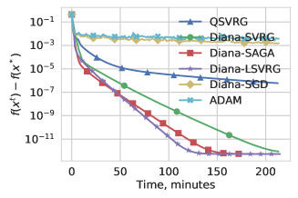
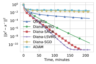
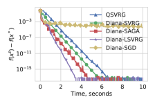
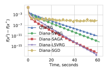
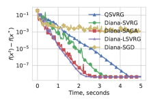
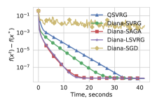
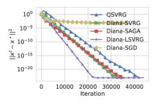
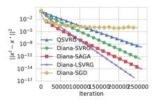
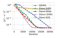
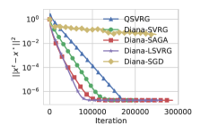
We illustrate the performance of the considered methods on standard logistic regression problems for binary classification. We regularize the loss with $\ell_{2}$-penalty, so the full objective is $\log(1+\exp(-b_{ij}A_{ij}^{\top}x))+\frac{\lambda_{2}}{2}\|x\|_{2}^{2}$, where $A_{ij},b_{ij}$ are data points and $\lambda_{2}$ is the regularization parameter. This problem is attractive because some of the methods to which we want to compare do not have convergence guarantees for non-convex or non-smooth objective. $\lambda_{2}$ is set to be of order $1/(nm)$. The datasets used are from the LIBSVM library Chang & Lin (2011).

We implement all methods in Python using MPI4PY Dalcin et al. (2011) for collective communication operations. We run all experiments on a machine with 24 Intel(R) Xeon(R) Gold 6146 CPU @ 3.20GHz cores. The cores are connected to two sockets, 12 cores to each of them, and we run workers and the parameter server on different cores. The communication is done either using 32- or 64-bit numbers, so the convergence is correspondingly up to precision $10^{-8}$ or $10^{-16}$ in different experiments.

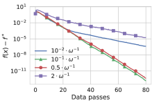
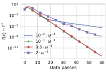
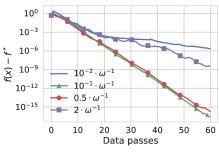
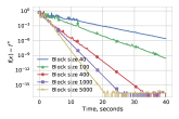
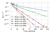
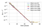
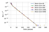
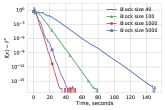
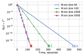
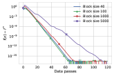
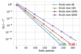
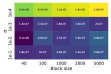
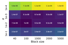
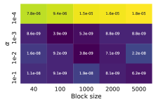
To have a trade-off between communication and iteration complexities, we use in most experiments the block quantization scheme with block sizes equal $n^{2}$, and in one additional experiments we explore what changes under different block sizes. We analyze the effect of changing the parameter $\alpha$ over different values in Figure 2 and find out that it is very easy to tune, and in most cases the speed of convergence is roughly the same unless $\alpha$ is set too close to 1 or to 0. For instance, we see almost no difference between choosing any element of $\{10^{-2},10^{-3},5\cdot 10^{-4}\}$ when $\omega^{-1}=2\cdot 10^{-2}$, although for tiny values the convergence becomes much slower. For more detailed consideration of block sizes and choices of $\alpha$ on a larger dataset see Figure 5.

We also provide a comparison between most relevant quantization method: QSVRG Alistarh et al. (2017), TernGrad-Adam and Diana Mishchenko et al. (2018) in Figure 3. Since TernGrad-Adam was the slowest in our experiments, we provide it only in Figure 1.

9 Conclusion

In this work we analyzed various distributed algorithms that support quantized communication between worker nodes. Our analysis is general, that is, not bound to a specific quantization scheme. This fact is especially interesting as we have showed that by choosing the quantization operator (respectively the introduced noise) in the right way, we obtain communication efficient schemes that converge as fast as their communication intensive counterparts. We develop the first variance reduced methods that support quantized communication and derive concise convergence rates for the strongly-convex, the convex and the non-convex setting.

Acknowledgments

The authors would like to thank Xun Qian for the careful checking of the proofs and for spotting several typos in the analysis.

Appendix A Extra Experiments

(a) $\ell_{\infty}$, $\lambda_{2}=2\cdot 10^{-1}$

(b) $\ell_{\infty}$, $\lambda_{2}=2\cdot 10^{-2}$

(c) $\ell_{\infty}$, $\lambda_{2}=2\cdot 10^{-1}$

(d) $\ell_{\infty}$, $\lambda_{2}=2\cdot 10^{-2}$

(e) $\ell_{2}$, $\lambda_{2}=2\cdot 10^{-1}$

(f) $\ell_{2}$, $\lambda_{2}=2\cdot 10^{-2}$

(g) $\ell_{2}$, $\lambda_{2}=2\cdot 10^{-1}$

(h) $\ell_{2}$, $\lambda_{2}=2\cdot 10^{-2}$

Figure 4: Experiments with Diana-SVRG and different block sizes applied to the Gisette dataset ($d=5000$) with $n=20$ workers. In the first two columns we show convergence over time and in the last two we show convergence over epochs. We used 1-bit random dithering with $\ell_{\infty}$ (first row) and $\ell_{2}$ norm and found out that even quantization with full vector quantization often does not slow down iteration complexity, but helps significantly with communication time. At the same time, $\ell_{2}$ dithering is noisier and yields a more significant impact of the block sizes on the iteration complexity. For each line in the plots, an optimal stepsize was found and we found out that larger block sizes require slightly smaller steps in case of $\ell_{2}$ random dithering. In all cases, we chose $\alpha$ to be $\frac{1}{2\omega}$, where $\omega$ was computed using the block size.

(a) SVRG

(b) SAGA

(c) L-SVRG

Figure 5: Functional gap after 20 epochs over the Gisette dataset ($d=5000$) with Diana-VR and different combinations of block sizes and $\alpha$ with $n=20$ workers. The same (optimal) stepsize is used in all cases with $\ell_{\infty}$ random dithering. For each cell, we average the results over 3 runs with the same parameters as the final accuracy is random. The best iteration performance is achieved using small blocks as expected, and the value of $\alpha$ does not matter much unless chosen too far from $\frac{1}{\omega+1}$. The values of $\frac{1}{\omega+1}$ for the columns from the left to the right approximately are $\{0.14,0.09,0.03,0.02,0.01\}$.

Appendix B Notation Table

To enhance the readers convenience when navigating to the extensive appendix, we here reiterate our notation:

General
${\rm E}\left[.\right],{\rm E}_{Q}\left[.\right]$	Expectation, Expectation over Quantization
$\mu$	Strong convexity constant	(4)
$L$	Smoothness constant	(5)
$\kappa$	condition number of problem $l/\mu$
$d$	Dimension of $x$ in $f(x)$
$n$	Number of function in finite sum
$f$	Objective to be minimized over set $\mathbb{R}^{d}$	(1), (8)
$Q(x)$	Quantization operator	(7)
$\omega$	Quantization parameter	(7)
$\operatorname{prox}$	Proximal operator
$x^{\star}$	Global minimizer of $f$
$f^{\star}$	function value in optimum $x^{\star}$
$R$	Regularizer	(8)
General Diana
$\sigma_{i}$’s	constants, upper bound on variance	(9)
$\alpha,\gamma$	parameters/ step sizes	Alg. 1
$\Psi^{k}$	Lyapunov function	Thm. 1
$c$	parameter of Lyapunov function	Thm. 1
VR-Diana
$\alpha,\gamma$	Parameters/ step sizes	Alg. 2
$m$	number of functions on each node	(11)
$\psi^{k}$	Lyapunov function for strongly convex case and convex case	Thm. 2
$H^{k},D^{k}$	Elements of Lyapunov function $\psi^{k}$	Thm. 2
$b,c$	Parameters of Lyapunov function $\psi^{k}$	Thm. 2
$R^{k}$	Lyapunov function for non-convex case	Thm. 5
$F^{k},W^{k}$	Elements of Lyapunov function $R^{k}$	Thm. 5
$c^{k},d^{k}$	Parameters of Lyapunov function $\psi^{k}$	Thm. 5
SVRG-Diana
$\alpha,\gamma$	Parameters/ step sizes	Alg. 3
$m$	number of functions on each node	(11)
$l$	Outer loop length for Algorithm 3	Alg. 3
$\{p_{r}\}_{r=0}^{l-1}$	coefficients for the reference point $z_{s}$	Alg. 3
$\psi^{k}$	Lyapunov function for strongly convex case and convex case	Thm. 6
$H^{k}$	Element of Lyapunov function $\psi^{k}$	(37)
$b$	Parameter of Lyapunov function $\psi^{k}$	(38)
$R^{k}$	Lyapunov function for non-convex case	Thm. 8
$F^{k},W^{k}$	Elements of Lyapunov function $R^{k}$	Thm. 8

Table 2: Summary of frequently used notation.

Appendix C Basic Identities and Inequalities

For random variable $X$ and any $y\in\mathbb{R}^{d}$, the variance can be decomposed as

$${\rm E}\left[\lVert X-{\rm E}\left[X\right]\rVert_{2}^{2}\right]={\rm E}\left[\lVert X-y\rVert_{2}^{2}\right]-{\rm E}\left[\lVert{\rm E}\left[X\right]-y\rVert_{2}^{2}\right]\,.$$ (12)

For any vectors $a_{1},a_{2},\dots,a_{k}\in\mathbb{R}^{d}$, we have as a consequence of Jensen’s inequality:

$$\left\|\sum_{i=1}^{k}a_{i}\right\|_{2}^{2}\leq k\sum_{i=1}^{k}\lVert a_{i}\rVert_{2}^{2}\,.$$ (13)

For any independent random variables $X_{1},X_{2},\cdots,X_{n}\in\mathbb{R}^{d}$ we have

$${\rm E}\left[\lVert\frac{1}{n}\sum_{i=1}^{n}\left(X_{i}-{\rm E}\left[X_{i}\right]\right)\rVert_{2}^{2}\right]=\frac{1}{n^{2}}\sum_{i=1}^{n}{\rm E}\left[\lVert X_{i}-{\rm E}\left[X_{i}\right]\rVert_{2}^{2}\right]$$ (14)

For a $L$-smooth and $\mu$-strongly convex function $f\colon\mathbb{R}^{d}\to\mathbb{R}$ we have

$$\left\langle\nabla f(x)-\nabla f(y),x-y\right\rangle\geq\frac{\mu L}{\mu+L}\lVert x-y\rVert_{2}^{2}+\frac{1}{\mu+L}\lVert\nabla f(x)-\nabla f(y)\rVert_{2}^{2}\,, \forall x,y\in\mathbb{R}^{d}\,.$$ (15)

For $\mu$-strongly convex function $f\colon\mathbb{R}^{d}\to\mathbb{R}$ we have

$$\left\langle\nabla f(x)-\nabla f(y),x-y\right\rangle\geq\mu\lVert x-y\rVert_{2}^{2}\,, \forall x,y\in\mathbb{R}^{d}\,.$$ (16)

The prox operator of a closed convex function is non-expansive. That is, for $\gamma>0$,

$$\lVert\operatorname{prox}_{\gamma R}(x)-\operatorname{prox}_{\gamma R}(y)\rVert \leq\lVert x-y\rVert\,, \forall x,y\in\mathbb{R}^{d}\,.$$ (17)

Throughout the whole appendix we use conditional expectation ${\rm E}\left[{\cal X}|x^{k},h_{i}^{k}\right]$ for DIANA and ${\rm E}\left[{\cal X}|x^{k},h_{i}^{k},w_{ij}^{k}\right]$ for VR-DIANA and ${\rm E}\left[{\cal X}|x^{k},h_{i}^{k},z^{s}\right]$ for SVRG-DIANA, but for simplicity, we will denote these expectations as ${\rm E}\left[{\cal X}\right]$. If ${\rm E}\left[{\cal X}\right]$ refers to unconditional expectation, it is directly mentioned.

Appendix D DIANA with general quantization operators, Proof of Theorem 1

Lemma 1.

For all iterations $k\geq 0$ of Algorithm 1 it holds

$${\rm E}_{Q}\left[\hat{g}^{k}\right] =g^{k}:=\frac{1}{n}\sum_{i=1}^{n}g_{i}^{k}\,, {\rm E}_{Q}\left[\lVert\hat{g}^{k}-g^{k}\rVert_{2}^{2}\right] \leq\frac{\omega}{n^{2}}\sum_{i=1}^{n}\lVert\Delta_{i}^{k}\rVert_{2}^{2}\,, {\rm E}\left[g^{k}\right] =\nabla f(x^{k})\,.$$ (18)

Furthermore, for $h^{\star}=\nabla f(x^{\star})$, $h_{i}^{\star}:=\nabla f_{i}(x^{\star})$

$${\rm E}\left[\lVert\hat{g}^{k}-h^{\star}\rVert_{2}^{2}\right] \leq\left(1+\frac{2\omega}{n}\right)\frac{1}{n}\sum_{i=1}^{n}{\rm E}\left[\lVert\nabla f_{i}(x^{k})-h_{i}^{\star}\rVert_{2}^{2}\right]+\left(1+\omega\right)\frac{\sigma^{2}}{n}+\frac{2\omega}{n^{2}}\sum_{i=1}^{n}{\rm E}\left[\lVert h_{i}^{\star}-h_{i}^{k}\rVert_{2}^{2}\right]\,.$$ (19)

Proof.

The first equation in (18) follows from the unbiasedness of the quantization operator. By the contraction property (7) we have

$${\rm E}_{Q}\left[\lVert\hat{g}_{i}^{k}-g_{i}^{k}\rVert_{2}^{2}\right]\leq\omega\lVert\Delta_{i}^{k}\rVert_{2}^{2}\,,$$

for every $i=1,\dots,n$ and the second relation in (18) follows from independence of $\hat{g}_{1}^{k},\dots,\hat{g}_{n}^{k}$. The last equality in (18) follows from the assumption that each $g_{i}^{k}$ is an unbiased estimate of $\nabla f_{i}(x^{k})$.

By applying two times the identity ${\rm E}\left[\lVert X-y\rVert_{2}^{2}\right]={\rm E}\left[\lVert X-{\rm E}\left[X\right]\rVert_{2}^{2}\right]+{\rm E}\left[\lVert{\rm E}\left[X\right]-y\rVert_{2}^{2}\right]$ for random variable $X$ and $y\in\mathbb{R}^{d}$, we get

$${\rm E}\left[\lVert\hat{g}^{k}-h^{\star}\rVert_{2}^{2}\right] \stackrel{{\scriptstyle\eqref{eq:variance}}}{{=}}{\rm E}\left[\lVert\hat{g}^{k}-g^{k}\rVert_{2}^{2}\right]+{\rm E}\left[\lVert g^{k}-h^{\star}\rVert_{2}^{2}\right]$$

$$\stackrel{{\scriptstyle\eqref{eq:variance}}}{{=}}{\rm E}\left[\lVert\hat{g}^{k}-g^{k}\rVert_{2}^{2}\right]+{\rm E}\left[\lVert g^{k}-\nabla f(x^{k})\rVert_{2}^{2}\right]+{\rm E}\left[\lVert\nabla f(x^{k})-h^{\star}\rVert_{2}^{2}\right]$$

and thus

$${\rm E}\left[\lVert\hat{g}^{k}-h^{\star}\rVert_{2}^{2}\right] \stackrel{{\scriptstyle\eqref{def:sigmai}+\eqref{eq:explain0}}}{{\leq}}\frac{\omega}{n^{2}}\sum_{i=1}^{n}{\rm E}\left[\lVert\Delta_{i}^{k}\rVert_{2}^{2}\right]+\frac{\sigma^{2}}{n}+{\rm E}\left[\lVert\nabla f(x^{k})-h^{\star}\rVert_{2}^{2}\right]\,.$$ (20)

Note that

$$\lVert\nabla f(x^{k})-h^{\star}\rVert_{2}^{2}\leq\frac{1}{n}\sum_{i=1}^{n}\lVert\nabla f_{i}(x^{k})-h_{i}^{\star}\rVert_{2}^{2}\,,$$

by Jensen’s inequality. Further,

$${\rm E}\left[\lVert\Delta_{i}^{k}\rVert_{2}^{2}\right] ={\rm E}\left[\lVert g_{i}^{k}-h_{i}^{k}\rVert_{2}^{2}\right]\stackrel{{\scriptstyle\eqref{eq:variance}}}{{=}}{\rm E}\left[\lVert\nabla f_{i}(x^{k})-h_{i}^{k}\rVert_{2}^{2}\right]+{\rm E}\left[\lVert\nabla f_{i}(x^{k})-g_{i}^{k}\rVert_{2}^{2}\right]$$

$$\stackrel{{\scriptstyle\eqref{def:sigmai}}}{{\leq}}{\rm E}\left[\lVert\nabla f_{i}(x^{k})-h_{i}^{k}\rVert_{2}^{2}\right]+\sigma_{i}^{2}$$

$$\stackrel{{\scriptstyle\eqref{eq:sum}}}{{\leq}}2{\rm E}\left[\lVert\nabla f_{i}(x^{k})-h_{i}^{\star}\rVert_{2}^{2}\right]+2{\rm E}\left[\lVert h_{i}^{\star}-h_{i}^{k}\rVert_{2}^{2}\right]+\sigma_{i}^{2}.$$

By summing up these bounds and plugging the result into (20), equation (19) follows. ∎

Lemma 2.

Let $\alpha(\omega+1)\leq 1$. For $i=1,\dots,n$, we can upper bound the second moment of $h_{i}^{k+1}$ as

$${\rm E}_{Q}\left[\lVert h_{i}^{k+1}-h_{i}^{\star}\rVert_{2}^{2}\right]\leq(1-\alpha)\lVert h_{i}^{k}-h_{i}^{\star}\rVert_{2}^{2}+\alpha\lVert\nabla f_{i}(x^{k})-h_{i}^{\star}\rVert_{2}^{2}+\alpha\sigma^{2}_{i}\,.$$ (21)

Proof.

Since $h_{i}^{k+1}=h_{i}^{k}+\alpha\hat{\Delta}_{i}^{k}$ we can decompose

$${\rm E}_{Q}\left[\lVert h_{i}^{k+1}-h_{i}^{\star}\rVert_{2}^{2}\right] ={\rm E}_{Q}\left[\lVert\alpha\hat{\Delta}_{i}^{k}+(h_{i}^{k}-h_{i}^{\star})\rVert_{2}^{2}\right]=\lVert h_{i}^{k}-h_{i}^{\star}\rVert_{2}^{2}+2{\rm E}_{Q}\left[\left\langle\alpha\hat{\Delta}_{i}^{k},h_{i}^{k}-h_{i}^{\star}\right\rangle\right]+{\rm E}_{Q}\left[\lVert\alpha\hat{\Delta}_{i}^{k}\rVert_{2}^{2}\right]$$

$$\stackrel{{\scriptstyle\eqref{def:Q}}}{{\leq}}\lVert h_{i}^{k}-h_{i}^{\star}\rVert_{2}^{2}+2\left\langle\alpha\Delta_{i}^{k},h_{i}^{k}-h_{i}^{\star}\right\rangle+\alpha^{2}(\omega+1)\lVert\Delta_{i}^{k}\rVert_{2}^{2}.$$

Let plug in the bound $(\omega+1)\alpha\leq 1$ and continue the derivation:

$${\rm E}_{Q}\left[\lVert h_{i}^{k+1}-h_{i}^{\star}\rVert_{2}^{2}\right] \leq\lVert h_{i}^{k}-h_{i}^{\star}\rVert_{2}^{2}+2\left\langle\alpha\Delta_{i}^{k},h_{i}^{k}-h_{i}^{\star}\right\rangle+\alpha\lVert\Delta_{i}^{k}\rVert_{2}^{2}$$

$$=\lVert h_{i}^{k}-h_{i}^{\star}\rVert_{2}^{2}+\alpha\left\langle g_{i}^{k}-h_{i}^{k},g_{i}^{k}+h_{i}^{k}-2h_{i}^{\star}\right\rangle$$

$$=\lVert h_{i}^{k}-h_{i}^{\star}\rVert_{2}^{2}+\alpha\lVert g_{i}^{k}-h_{i}^{\star}\rVert_{2}^{2}-\alpha\lVert h_{i}^{k}-h_{i}^{\star}\rVert_{2}^{2}$$

$$\leq(1-\alpha)\lVert h_{i}^{k}-h_{i}^{\star}\rVert_{2}^{2}+\alpha\lVert g_{i}^{k}-h_{i}^{\star}\rVert_{2}^{2}\qed.$$

The second term can be further upper-bounded by $\lVert\nabla f_{i}(x^{k})-h_{i}^{\star}\rVert_{2}^{2}+\sigma^{2}_{i}$, where we use (12), which concludes the proof.

Proof of Theorem 1.

If $x^{\star}$ is a solution of (1), then $x^{\star}=\operatorname{prox}_{\gamma R}(x^{\star}-\gamma h^{\star})$ (for $\gamma>0$. Using this identity together with the non-expansiveness of the prox operator we can bound the first term of the Lyapunov function:

$${\rm E}\left[\lVert x^{k+1}-x^{\star}\rVert_{2}^{2}\right] ={\rm E}\left[\lVert\operatorname{prox}_{\gamma R}(x^{k}-\gamma\hat{g}^{k})-\operatorname{prox}_{\gamma R}(x^{\star}-\gamma h^{\star})\rVert_{2}^{2}\right]$$

$$\leq{\rm E}\left[\lVert x^{k}-\gamma\hat{g}^{k}-(x^{\star}-\gamma h^{\star}))\rVert_{2}^{2}\right]$$

$$={\rm E}\left[\lVert x^{k}-x^{\star}\rVert_{2}^{2}\right]-2\gamma{\rm E}\left[\left\langle\hat{g}^{k}-h^{\star},x^{k}-x^{\star}\right\rangle\right]+\gamma^{2}{\rm E}\left[\lVert\hat{g}^{k}-h^{\star}\rVert_{2}^{2}\right]$$

$$={\rm E}\left[\lVert x^{k}-x^{\star}\rVert_{2}^{2}\right]-2\gamma\left\langle\nabla f(x^{k})-h^{\star},x^{k}-x^{\star}\right\rangle+\gamma^{2}{\rm E}\left[\lVert\hat{g}^{k}-h^{\star}\rVert_{2}^{2}\right].$$

It is high time to use strong convexity of each component $f_{i}$:

$${\rm E}\left[\left\langle\nabla f(x^{k})-h^{\star},x^{k}-x^{\star}\right\rangle\right] =\frac{1}{n}\sum_{i=1}^{n}{\rm E}\left[\left\langle\nabla f_{i}(x^{k})-h_{i}^{\star},x^{k}-x^{\star}\right\rangle\right]$$

$$\stackrel{{\scriptstyle\eqref{eq:coerc}}}{{\geq}}\frac{1}{n}\sum_{i=1}^{n}\left(\frac{\mu L}{\mu+L}{\rm E}\left[\lVert x^{k}-x^{\star}\rVert_{2}^{2}\right]+\frac{1}{\mu+L}{\rm E}\left[\lVert\nabla f_{i}(x^{k})-h_{i}^{\star}\rVert_{2}^{2}\right]\right)$$

$$=\frac{\mu L}{\mu+L}{\rm E}\left[\lVert x^{k}-x^{\star}\rVert_{2}^{2}\right]+\frac{1}{\mu+L}\frac{1}{n}\sum_{i=1}^{n}{\rm E}\left[\lVert\nabla f_{i}(x^{k})-h_{i}^{\star}\rVert_{2}^{2}\right]\,.$$

Hence,

$${\rm E}\left[\lVert x^{k+1}-x^{\star}\rVert_{2}^{2}\right]\leq\left(1-\frac{2\gamma\mu L}{\mu+L}\right){\rm E}\left[\lVert x^{k}-x^{\star}\rVert_{2}^{2}\right]-\frac{2\gamma}{\mu+L}\frac{1}{n}\sum_{i=1}^{n}{\rm E}\left[\lVert\nabla f_{i}(x^{k})-h_{i}^{\star}\rVert_{2}^{2}\right]+\gamma^{2}{\rm E}\left[\lVert\hat{g}^{k}-h^{\star}\rVert_{2}^{2}\right]$$

and by Lemma 1:

$$\begin{split}{\rm E}\left[\lVert x^{k+1}-x^{\star}\rVert_{2}^{2}\right]&\stackrel{{\scriptstyle\eqref{eq:explain2}}}{{\leq}}\left(1-\frac{2\gamma\mu L}{\mu+L}\right){\rm E}\left[\lVert x^{k}-x^{\star}\rVert_{2}^{2}\right]+\left(\gamma^{2}\left(1+\frac{2\omega}{n}\right)-\frac{2\gamma}{\mu+L}\right)\frac{1}{n}\sum_{i=1}^{n}{\rm E}\left[\lVert\nabla f_{i}(x^{k})-h_{i}^{\star}\rVert_{2}^{2}\right]\\ &\qquad+\gamma^{2}\left(1+\omega\right)\frac{\sigma^{2}}{n}+\left(\gamma^{2}\frac{2\omega}{n}\right)\frac{1}{n}\sum_{i=1}^{n}{\rm E}\left[\lVert h_{i}^{k}-h_{i}^{\star}\rVert_{2}^{2}\right]\,.\end{split}$$ (22)

Now let us consider the Lyapunov function:

$$\begin{split}{\rm E}\left[\Psi^{k+1}\right]&\stackrel{{\scriptstyle\eqref{eq:hdecrement}+\eqref{eq:6943}}}{{\leq}}\left(1-\frac{2\gamma\mu L}{\mu+L}\right){\rm E}\left[\lVert x^{k}-x^{\star}\rVert_{2}^{2}\right]+\gamma^{2}\left(1+\omega\right)\frac{\sigma^{2}}{n}\\ &\qquad+\left(\gamma^{2}\left(1+\frac{2\omega}{n}+c\alpha\right)-\frac{2\gamma}{\mu+L}\right)\frac{1}{n}\sum_{i=1}^{n}{\rm E}\left[\lVert\nabla f_{i}(x^{k})-h_{i}^{\star}\rVert_{2}^{2}\right]\\ &\qquad+\gamma^{2}\left(\frac{2\omega}{n}+(1-\alpha)c\right)\frac{1}{n}\sum_{i=1}^{n}\lVert h_{i}^{k}-h_{i}^{\star}\rVert_{2}^{2}+\gamma^{2}c\alpha\sigma^{2}\,.\end{split}$$ (23)

In view of the assumption on $\gamma$ we have $\gamma^{2}\left(1+\frac{2\omega}{n}+c\alpha\right)-\frac{2\gamma}{\mu+L}\leq 0$. Since each $f_{i}$ is $\mu$-strongly convex, we have $\mu\lVert x^{k}-x^{\star}\rVert_{2}^{2}\stackrel{{\scriptstyle\eqref{eq:coerc2}}}{{\leq}}\left\langle\nabla f_{i}(x^{k})-h_{i}^{\star},x^{k}-x^{\star}\right\rangle$ and thus $\mu^{2}\lVert x^{k}-x^{\star}\rVert_{2}^{2}\leq\lVert\nabla f_{i}(x^{k})-h_{i}^{\star}\rVert_{2}^{2}$ with Cauchy-Schwarz. Using these observations we can absorb the third term in (23) in the first one:

$$\begin{split}{\rm E}\left[\Psi^{k+1}\right]&\leq\left(1-2\gamma\mu+\mu^{2}\gamma^{2}\left(1+\frac{2\omega}{n}+c\alpha\right)\right){\rm E}\left[\lVert x^{k}-x^{\star}\rVert_{2}^{2}\right]+\gamma^{2}\left(c\alpha+\frac{\omega+1}{n}\right)\sigma^{2}\\ &\qquad+\gamma^{2}\left(\frac{2\omega}{n}+(1-\alpha)c\right)\frac{1}{n}\sum_{i=1}^{n}\lVert h_{i}^{k}-h_{i}^{\star}\rVert_{2}^{2}\,.\end{split}$$

By the first assumption on $\gamma$ it follows $\left(1-2\gamma\mu+\mu^{2}\gamma^{2}\left(1+\frac{2\omega}{n}+c\alpha\right)\right)\leq(1-\gamma\mu)$. By the assumption on $c$ we have $\left(\frac{2\omega}{n}+(1-\alpha)c\right)\leq\left(1-\frac{\alpha}{2}\right)c$. An the second assumption on $\gamma$ implies $\left(1-\frac{\alpha}{2}\right)\leq(1-\gamma\mu)$. Thus

$${\rm E}\left[\Psi^{k+1}\right]\leq(1-\gamma\mu)\Psi^{k}+\gamma^{2}\left(1+\frac{\omega}{n}\right)\frac{\sigma^{2}}{n}\,.$$

Unrolling the recurrence and the estimate $\sum_{\ell=0}^{k-1}(1-\gamma\mu)^{k}\leq\frac{1}{\mu\gamma}$ for all $k\geq 1$ leads to

$${\rm E}\left[\Psi^{k}\right]\leq(1-\gamma\mu)^{k}\Psi^{0}+\frac{\gamma}{\mu}\left(c\alpha+\frac{\omega+1}{n}\right)\sigma^{2}\leq(1-\gamma\mu)^{k}\Psi^{0}+\frac{2}{\mu(\mu+L)}\sigma^{2}\,,$$

by the first assumption on $\gamma$. ∎

Appendix E Variance Reduced Diana—L-SVRG method and SAGA proof

Lemma 3.

For all iterates $k\leq 0$ of Algorithm 2, it holds that $g_{i}^{k}$ is an unbiased estimate of the local gradient $\nabla f_{i}(x^{k})$

$${\rm E}\left[g_{i}^{k}\right]=\nabla f_{i}(x^{k})$$

and $g^{k}$ is that of the full gradient $\nabla f(x^{k})$:

$${\rm E}\left[g^{k}\right]=\nabla f(x^{k}).$$

Proof.

It is a straightforward consequence of how we define sampling:

$${\rm E}\left[g_{i}^{k}\right]={\rm E}\left[\nabla f_{ij_{i}^{k}}(x^{k})-\nabla f_{ij_{i}^{k}}(w_{ik_{i}^{k}}^{k})+\mu_{i}^{k}\right]=\nabla f_{i}(x^{k})-\mu_{i}^{k}+\mu_{i}^{k}=\nabla f_{i}(x^{k}).$$

Similarly,

$${\rm E}\left[g^{k}\right]=\frac{1}{n}\sum\limits_{i=1}^{n}{\rm E}\left[Q(g_{i}^{k}-h_{i}^{k})+h_{i}^{k}\right]=\frac{1}{n}\sum\limits_{i=1}^{n}{\rm E}\left[g_{i}^{k}-h_{i}^{k}+h_{i}^{k}\right]=\frac{1}{n}\sum\limits_{i=1}^{n}\nabla f_{i}(x^{k})=\nabla f(x^{k}).$$

∎

E.1 Strongly convex case

Lemma 4.

We can upper bound the second moment of $x^{k}$ in the following way

$${\rm E}\left[\lVert x^{k+1}-x^{\star}\rVert_{2}^{2}\right]\leq\lVert x^{k}-x^{\star}\rVert_{2}^{2}(1-\mu\gamma)+2\gamma(f^{\star}-f(x^{k}))+\gamma^{2}{\rm E}\left[\lVert g^{k}\rVert_{2}^{2}\right].$$ (24)

Proof.

$${\rm E}\left[\lVert x^{k+1}-x^{\star}\rVert_{2}^{2}\right] ={\rm E}\left[\lVert x^{k}-x^{\star}\rVert_{2}^{2}+2\gamma\left\langle g^{k},x^{\star}-x^{k}\right\rangle+\gamma^{2}\lVert g^{k}\rVert_{2}^{2}\right]$$

$$=\lVert x^{k}-x^{\star}\rVert_{2}^{2}+2\gamma\left\langle\nabla f(x^{k}),x^{\star}-x^{k}\right\rangle+\gamma^{2}{\rm E}\left[\lVert g^{k}\rVert_{2}^{2}\right]$$

$$\overset{\eqref{def:strongconvex}}{\leq}\lVert x^{k}-x^{\star}\rVert_{2}^{2}+2\gamma\left(f^{\star}-f(x^{k})-\frac{\mu}{2}\lVert x^{k}-x^{\star}\rVert_{2}^{2}\right)+\gamma^{2}{\rm E}\left[\lVert g^{k}\rVert_{2}^{2}\right]$$

$$=\lVert x^{k}-x^{\star}\rVert_{2}^{2}(1-\mu\gamma)+2\gamma(f^{\star}-f(x^{k}))+\gamma^{2}{\rm E}\left[\lVert g^{k}\rVert_{2}^{2}\right],$$

where the first equation follows from the definition of $x^{k+1}$ in Algorithm 2. ∎

Lemma 5.

Let $\alpha(\omega+1)\leq 1$. We can upper bound $H^{k+1}$ in the following way

$${\rm E}\left[H^{k+1}\right]\leq(1-\alpha)H^{k}+\frac{2\alpha}{m}D^{k}+8\alpha Ln\left(f(x^{k})-f^{\star}\right),$$ (25)

where

$$H^{k}\overset{\text{def}}{=}\sum\limits_{i=1}^{n}\lVert h_{i}^{k}-\nabla f_{i}(x^{\star})\rVert_{2}^{2}$$ (26)

and

$$D^{k}\overset{\text{def}}{=}\sum\limits_{i=1}^{n}\sum\limits_{j=1}^{m}\lVert\nabla f_{ij}(w_{ij}^{k})-\nabla f_{ij}(x^{\star})\rVert_{2}^{2}.$$ (27)

Proof.

$${\rm E}\left[H^{k+1}\right] ={\rm E}\left[\sum\limits_{i=1}^{n}\lVert h_{i}^{k+1}-\nabla f_{i}(x^{\star})\rVert_{2}^{2}\right]$$

$$=\sum\limits_{i=1}^{n}\lVert h_{i}^{k}-\nabla f_{i}(x^{\star})\rVert_{2}^{2}$$

$$\qquad+\sum\limits_{i=1}^{n}{\rm E}\left[2\left\langle\alpha Q(g_{i}^{k}-h_{i}^{k}),h_{i}^{k}-\nabla f_{i}(x^{\star})\right\rangle+\alpha^{2}\lVert Q(g_{i}^{k}-h_{i}^{k})\rVert_{2}^{2}\right]$$

$$\leq H^{k}+\sum\limits_{i=1}^{n}{\rm E}\left[2\alpha\left\langle g_{i}^{k}-h_{i}^{k},h_{i}^{k}-\nabla f_{i}(x^{\star})\right\rangle+\alpha\left(\alpha\cdot(\omega+1)\right)\lVert g_{i}^{k}-h_{i}^{k}\rVert_{2}^{2}\right]$$

$$\leq H^{k}+{\rm E}\left[\sum\limits_{i=1}^{n}\alpha\left\langle g_{i}^{k}-h_{i}^{k},g_{i}^{k}+h_{i}^{k}-2\nabla f_{i}(x^{\star})\right\rangle\right]$$

$$=H^{k}+{\rm E}\left[\sum\limits_{i=1}^{n}\alpha\left(\lVert g_{i}^{k}-\nabla f_{i}(x^{\star})\rVert_{2}^{2}-\lVert h_{i}^{k}-\nabla f_{i}(x^{\star})\rVert_{2}^{2}\right)\right]$$

$$=H^{k}(1-\alpha)+{\rm E}\left[\sum\limits_{i=1}^{n}\alpha\left(\lVert g_{i}^{k}-\nabla f_{i}(x^{\star})\rVert_{2}^{2}\right)\right]$$

$$\overset{\eqref{eq:sum}}{\leq}H^{k}(1-\alpha)+\sum\limits_{i=1}^{n}\left(2\alpha{\rm E}\left[\lVert g_{i}^{k}-\nabla f_{i}(x^{k})\rVert_{2}^{2}\right]+2\alpha\lVert\nabla f_{i}(x^{k})-\nabla f_{i}(x^{\star})\rVert_{2}^{2}\right)$$

$$\overset{\text{Alg.}~{}\ref{alg:VR-DIANA}}{=}H^{k}(1-\alpha)+\sum\limits_{i=1}^{n}{\rm E}\left[2\alpha\lVert\nabla f_{ij_{i}^{k}}(x^{k})-\nabla f_{ij_{i}^{k}}(w_{ij_{i}^{k}}^{k})-{\rm E}\left[\nabla f_{ij_{i}^{k}}(x^{k})-\nabla f_{ij_{i}^{k}}(w_{ij_{i}^{k}}^{k})\right]\rVert_{2}^{2}\right]$$

$$\quad+2\alpha\sum\limits_{i=1}^{n}\lVert\nabla f_{i}(x^{k})-\nabla f_{i}(x^{\star})\rVert_{2}^{2}$$

$$\overset{\eqref{eq:variance}}{\leq}H^{k}(1-\alpha)+\sum\limits_{i=1}^{n}\left({\rm E}\left[2\alpha\lVert\nabla f_{ij_{i}^{k}}(x^{k})-\nabla f_{ij_{i}^{k}}(w_{ij_{i}^{k}}^{k})\rVert_{2}^{2}\right]+2\alpha\lVert\nabla f_{i}(x^{k})-\nabla f_{i}(x^{\star})\rVert_{2}^{2}\right)$$

$$\overset{\eqref{eq:sum}}{\leq}H^{k}(1-\alpha)+\frac{2\alpha}{m}\sum\limits_{i=1}^{n}\sum\limits_{j=1}^{m}\left(\lVert\nabla f_{ij}(x^{k})-\nabla f_{ij}(x^{\star})\rVert_{2}^{2}+\lVert\nabla f_{ij}(w_{ij}^{k})-\nabla f_{ij}(x^{\star})\rVert_{2}^{2}\right)$$

$$\quad+2\alpha\sum\limits_{i=1}^{n}\lVert\nabla f_{i}(x^{k})-\nabla f_{i}(x^{\star})\rVert_{2}^{2}$$

$$\overset{\eqref{def:smoothness}}{\leq}H^{k}(1-\alpha)+\frac{2\alpha}{m}\sum\limits_{i=1}^{n}\sum\limits_{j=1}^{m}\lVert\nabla f_{ij}(w_{ij}^{k})-\nabla f_{ij}(x^{\star})\rVert_{2}^{2}+8\alpha Ln\left(f(x^{k})-f^{\star}\right)$$

$$=H^{k}(1-\alpha)+\frac{2\alpha}{m}D^{k}+8\alpha Ln\left(f(x^{k})-f^{\star}\right),$$

where the second equality uses definition of $h_{i}^{k+1}$ in Algorithm 2 and the first inequality follows from $\alpha(\omega+1)\leq 1$. ∎

Lemma 6.

We can upper bound $D^{k+1}$ in the following way

$${\rm E}\left[D^{k+1}\right]\leq D^{k}\left(1-\frac{1}{m}\right)+2Ln(f(x^{k})-f^{\star}).$$ (28)

Proof.

$${\rm E}\left[D^{k+1}\right] =\sum\limits_{i=1}^{n}\sum\limits_{j=1}^{m}{\rm E}\left[\lVert\nabla f_{ij}(w_{ij}^{k+1})-\nabla f_{ij}(x^{\star})\rVert_{2}^{2}\right]$$

$$=\sum\limits_{i=1}^{n}\sum\limits_{j=1}^{m}\left[\left(1-\frac{1}{m}\right)\lVert\nabla f_{ij}(w_{ij}^{k})-\nabla f_{ij}(x^{\star})\rVert_{2}^{2}+\frac{1}{m}\lVert\nabla f_{ij}(x^{k})-\nabla f_{ij}(x^{\star})\rVert_{2}^{2}\right]$$

$$\overset{\eqref{def:smoothness}}{\leq}D^{k}\left(1-\frac{1}{m}\right)+2Ln(f(x^{k})-f^{\star}),$$

where the second equality uses definition of $w_{ij}^{k+1}$ in Algorithm 2. ∎

Lemma 7.

We can upper bound the second moment of the $g^{k}$ in the following way

$${\rm E}\left[\lVert g^{k}\rVert_{2}^{2}\right]\leq 2L(f(x^{k})-f^{\star})\left(1+\frac{4\omega+2}{n}\right)+\frac{2\omega}{mn^{2}}D^{k}+\frac{2(\omega+1)}{n^{2}}H^{k}.$$ (29)

Proof.

$${\rm E}_{Q}\left[\lVert g^{k}\rVert_{2}^{2}\right] \overset{\eqref{eq:variance}}{=}\underbrace{\lVert{\rm E}_{Q}\left[g^{k}\right]\rVert_{2}^{2}}_{T_{1}}+\underbrace{{\rm E}_{Q}\left[\lVert g^{k}-{\rm E}_{Q}\left[g^{k}\right]\rVert_{2}^{2}\right]}_{T_{2}}.$$

We proceed with upper bounding terms $T_{1}$ and $T_{2}$ separately. For $T_{1}$ we can use definition of $g^{k}$ in order to obtain

$$T_{1} =\lVert\frac{1}{n}\sum\limits_{i=1}^{n}{\rm E}_{Q}\left[Q(g_{i}^{k}-h_{i}^{k})+h_{i}^{k}\right]\rVert_{2}^{2}=\lVert\frac{1}{n}\sum\limits_{i=1}^{n}g_{i}^{k}\rVert_{2}^{2}$$

and

$$T_{2} ={\rm E}_{Q}\left[\lVert\frac{1}{n}\sum\limits_{i=1}^{n}Q(g_{i}^{k}-h_{i}^{k})-(g_{i}^{k}-h_{i}^{k})\rVert_{2}^{2}\right]$$

$$\overset{\eqref{eq:indep}}{=}\frac{1}{n^{2}}\sum\limits_{i=1}^{n}{\rm E}_{Q}\left[\lVert Q(g_{i}^{k}-h_{i}^{k})-(g_{i}^{k}-h_{i}^{k})\rVert_{2}^{2}\right]$$

$$\overset{\eqref{def:Q}}{\leq}\frac{\omega}{n^{2}}\sum\limits_{i=1}^{n}\lVert g_{i}^{k}-h_{i}^{k}\rVert_{2}^{2}.$$

Let us calculate full expectations conditioned on previous iteration:

$${\rm E}\left[T_{2}\right] =\frac{\omega}{n^{2}}\sum\limits_{i=1}^{n}{\rm E}\left[\lVert g_{i}^{k}-h_{i}^{k}\rVert_{2}^{2}\right]=\frac{\omega}{n^{2}}\sum\limits_{i=1}^{n}\left(\lVert{\rm E}\left[g_{i}^{k}-h_{i}^{k}\right]\rVert_{2}^{2}+{\rm E}\left[\lVert g_{i}^{k}-h_{i}^{k}-{\rm E}\left[g_{i}^{k}-h_{i}^{k}\right]\rVert_{2}^{2}\right]\right)$$

$$=\frac{\omega}{n^{2}}\sum\limits_{i=1}^{n}\left(\lVert\nabla f_{i}(x^{k})-h_{i}^{k}\rVert_{2}^{2}+{\rm E}\left[\lVert g_{i}^{k}-\nabla f_{i}(x^{k})\rVert_{2}^{2}\right]\right)$$

$$=\frac{\omega}{n^{2}}\sum\limits_{i=1}^{n}\left(\lVert\nabla f_{i}(x^{k})-h_{i}^{k}\rVert_{2}^{2}+{\rm E}\left[\lVert\nabla f_{ij_{i}^{k}}(x^{k})-\nabla f_{ij_{i}^{k}}(w_{ij_{i}^{k}}^{k})-{\rm E}\left[\nabla f_{ij_{i}^{k}}(x^{k})-\nabla f_{ij_{i}^{k}}(w_{ij_{i}^{k}}^{k})\right]\rVert_{2}^{2}\right]\right)$$

$$\overset{\eqref{eq:variance}}{\leq}\frac{\omega}{n^{2}}\sum\limits_{i=1}^{n}\left(\lVert\nabla f_{i}(x^{k})-h_{i}^{k}\rVert_{2}^{2}+{\rm E}\left[\lVert\nabla f_{ij_{i}^{k}}(x^{k})-\nabla f_{ij_{i}^{k}}(w_{ij_{i}^{k}}^{k})\rVert_{2}^{2}\right]\right)$$

$$\overset{\eqref{eq:sum}}{\leq}\frac{2\omega}{n^{2}}\sum\limits_{i=1}^{n}\left(\lVert h_{i}^{k}-\nabla f_{i}(x^{\star})\rVert_{2}^{2}+\lVert\nabla f_{i}(x^{k})-\nabla f_{i}(x^{\star})\rVert_{2}^{2}\right)$$

$$\qquad+\frac{2\omega}{mn^{2}}\sum\limits_{i=1}^{n}\sum\limits_{j=1}^{m}\left(\lVert\nabla f_{ij}(w_{ij}^{k})-\nabla f_{ij}(x^{\star})\rVert_{2}^{2}+\lVert\nabla f_{ij}(x^{k})-\nabla f_{ij}(x^{\star})\rVert_{2}^{2}\right)$$

$$\overset{\eqref{def:smoothness}}{\leq}\frac{2\omega}{n^{2}}H^{k}+\frac{2\omega}{mn^{2}}D^{k}+\frac{8L\omega}{n}(f(x^{k})-f^{\star})$$

The other term follows in a similar way:

$${\rm E}\left[T_{1}\right] ={\rm E}\left[\lVert\frac{1}{n}\sum\limits_{i=1}^{n}g_{i}^{k}\rVert_{2}^{2}\right]=\lVert\frac{1}{n}\sum\limits_{i=1}^{n}{\rm E}\left[g_{i}^{k}\right]\rVert_{2}^{2}+{\rm E}\left[\lVert\frac{1}{n}\sum\limits_{i=1}^{n}\left(g_{i}^{k}-{\rm E}\left[g_{i}^{k}\right]\right)\rVert_{2}^{2}\right]$$

$$=\lVert\nabla f(x^{k})\rVert_{2}^{2}+\frac{1}{n^{2}}\sum\limits_{i=1}^{n}{\rm E}\left[\lVert g_{i}^{k}-\nabla f_{i}(x^{k})\rVert_{2}^{2}\right]$$

$$\overset{\eqref{def:smoothness}}{\leq}2L(f(x^{k})-f^{\star})+\frac{1}{n^{2}}\sum\limits_{i=1}^{n}{\rm E}\left[\lVert\nabla f_{ij_{i}^{k}}(x^{k})-\nabla f_{ij_{i}^{k}}(w_{ij_{i}^{k}}^{k})-{\rm E}\left[\nabla f_{ij_{i}^{k}}(x^{k})-\nabla f_{ij_{i}^{k}}(w_{ij_{i}^{k}}^{k})\right]\rVert_{2}^{2}\right]$$

$$\overset{\eqref{eq:variance}}{\leq}2L(f(x^{k})-f^{\star})+\frac{1}{n^{2}}\sum\limits_{i=1}^{n}{\rm E}\left[\lVert\nabla f_{ij_{i}^{k}}(x^{k})-\nabla f_{ij_{i}^{k}}(w_{ij_{i}^{k}}^{k})\rVert_{2}^{2}\right]$$

$$\overset{\text{Alg.}~{}\ref{alg:VR-DIANA}}{=}2L(f(x^{k})-f^{\star})+\frac{1}{mn^{2}}\sum\limits_{i=1}^{n}\sum\limits_{j=1}^{m}\lVert\nabla f_{ij}(x^{k})-\nabla f_{ij}(w_{ij}^{k})\rVert_{2}^{2}$$

$$\overset{\eqref{eq:sum}}{\leq}2L(f(x^{k})-f^{\star})+\frac{2}{mn^{2}}\sum\limits_{i=1}^{n}\sum\limits_{j=1}^{m}\left(\lVert\nabla f_{ij}(w_{ij}^{k})-\nabla f_{ij}(x^{\star})\rVert_{2}^{2}+\lVert\nabla f_{ij}(x^{k})-\nabla f_{ij}(x^{\star})\rVert_{2}^{2}\right)$$

$$\overset{\eqref{def:smoothness}}{\leq}(f(x^{k})-f^{\star})\left(2L+\frac{4L}{n}\right)+\frac{2}{mn^{2}}D^{k}.$$

Now, summing ${\rm E}\left[T_{1}\right]$ and ${\rm E}\left[T_{2}\right]$ we get

$${\rm E}\left[\lVert g^{k}\rVert_{2}^{2}\right] ={\rm E}\left[T_{1}+T_{2}\right]\leq(f(x^{k})-f^{\star})\left(2L+\frac{4L}{n}\right)+\frac{2}{mn^{2}}D^{k}$$

$$\quad+\frac{2\omega}{n^{2}}H^{k}+\frac{2\omega}{mn^{2}}D^{k}+\frac{8L\omega}{n}(f(x^{k})-f^{\star})$$

$$\leq(f(x^{k})-f^{\star})\left(2L+\frac{4L}{n}+\frac{8L\omega}{n}\right)+\frac{2\omega}{n^{2}}H^{k}+\frac{2(\omega+1)}{mn^{2}}D^{k},$$

which concludes the proof. ∎

Proof of Theorem 2.

Combining all lemmas together we may finalize proof. By the definition of Lyapunov function we have

$${\rm E}\left[\psi^{k+1}\right] ={\rm E}\left[\lVert x^{k+1}-x^{\star}\rVert_{2}^{2}+b\gamma^{2}H^{k+1}+c\gamma^{2}D^{k+1}\right]$$

$$\overset{\eqref{lem:up_x_k_VR}}{\leq}\lVert x^{k}-x^{\star}\rVert_{2}^{2}(1-\mu\gamma)+2\gamma(f^{\star}-f(x^{k}))+\gamma^{2}{\rm E}\left[\lVert g^{k}\rVert_{2}^{2}\right]+{\rm E}\left[b\gamma^{2}H^{k+1}+c\gamma^{2}D^{k+1}\right]$$

$$\overset{\eqref{lem:up_H_VR}+\eqref{lem:up_D_VR}+\eqref{lem:up_g_VR}}{\leq}\lVert x^{k}-x^{\star}\rVert_{2}^{2}(1-\mu\gamma)+2\gamma(f^{\star}-f(x^{k}))$$

$$\quad+\gamma^{2}\left(2L(f(x^{k})-f^{\star})\left(1+\frac{4\omega+2}{n}\right)+\frac{2(\omega+1)}{mn^{2}}D^{k}+\frac{2\omega}{n^{2}}H^{k}\right)$$

$$\quad+b\gamma^{2}\left(H^{k}(1-\alpha)+\frac{2\alpha}{m}D^{k}+8\alpha Ln\left(f(x^{k})-f^{\star}\right)\right)+c\gamma^{2}\left(D^{k}\left(1-\frac{1}{m}\right)+2Ln(f(x^{k})-f^{\star})\right)$$

$$=\lVert x^{k}-x^{\star}\rVert_{2}^{2}(1-\mu\gamma)+b\gamma^{2}H^{k}\left(1-\alpha+\frac{2\omega}{bn^{2}}\right)+c\gamma^{2}D^{k}\left(1-\frac{1}{m}+\frac{2b\alpha}{cm}+\frac{2(\omega+1)}{mn^{2}c}\right)$$

$$\quad+(f^{\star}-f(x^{k}))\left(2\gamma-2L\gamma^{2}\left[1+\frac{4\omega+2}{n}+cn+4b\alpha n\right]\right).$$ (30)

Now, choosing $b=\frac{4(\omega+1)}{\alpha n^{2}}$ and $c=\frac{16(\omega+1)}{n^{2}}$ , we get

$${\rm E}\left[\psi^{k+1}\right] \leq\lVert x^{k}-x^{\star}\rVert_{2}^{2}(1-\mu\gamma)+b\gamma^{2}H^{k}\left(1-\frac{\alpha}{2}\right)+c\gamma^{2}D^{k}\left(1-\frac{3}{8m}\right)$$

$$+(f^{\star}-f(x^{k}))\left(2\gamma-2L\gamma^{2}\left[1+\frac{36(\omega+1)}{n}\right]\right).$$

Setting $\gamma=\frac{1}{L\left(1+36(\omega+1)/n\right)}$ gives

$$E{\psi^{k+1}} \leq\lVert x^{k}-x^{\star}\rVert_{2}^{2}\left(1-\frac{\mu}{L\left(1+36(\omega+1)/n\right)}\right)+b\gamma^{2}H^{k}\left(1-\frac{\alpha}{2}\right)+c\gamma^{2}D^{k}\left(1-\frac{3}{8m}\right),$$

which concludes the proof. ∎

E.2 Convex case

Proof of Theorem 3.

Using (30) ($\mu=0$) assuming that $\alpha\geq\frac{2w}{bn^{2}}$ and $1\geq\frac{2b\alpha}{c}+\frac{2w}{cn^{2}}$, we obtain

$${\rm E}\left[\lVert x^{k+1}-x^{\star}\rVert_{2}^{2}+b\gamma^{2}H^{k+1}+c\gamma^{2}D^{k+1}\right]$$

$$\quad\leq\lVert x^{k}-x^{\star}\rVert_{2}^{2}+b\gamma^{2}H^{k}+c\gamma^{2}D^{k}+(f^{\star}-f(x^{k}))\left(2\gamma-2L\gamma^{2}\left[1+\frac{28\omega}{n}\right]\right),$$

which implies

$$(f(x^{k})-f^{\star})\left(2\gamma-2L\gamma^{2}\left[1+\frac{128\omega}{n}\right]\right)=\psi^{k}-{\rm E}\left[\psi^{k+1}\right],$$

which after removing conditional expectation can be summed over all iterations $1,2,\ldots,k$ and one has

$${\rm E}\left[f(x^{a})-f^{\star}\right]\leq\frac{\psi_{0}}{2k\left(\gamma-L\gamma^{2}\left[1+\frac{36(\omega+1)}{n}\right]\right)},$$

where index $a$ is uniformly at random picked from ${1,2,\cdots,k}$ ,which concludes the proof. ∎

E.3 Non-convex case

Theorem 5.

Consider Algorithm 2 with $\omega$-quantization $Q$, and stepsize $\alpha\leq\frac{1}{\omega+1}$. Choose any $p>0$ (which will appear in sequence $c^{k}$ below) to consider the following Lyapunov function

$$R^{k}=f(x^{k})+c^{k}W^{k}+d^{k}F^{k},$$

where

$$W^{k} =\frac{1}{mn}\sum\limits_{i=1}^{n}\sum\limits_{j=1}^{m}\lVert x^{k}-w_{ij}^{k}\rVert_{2}^{2}\,$$

$$F^{k} =\frac{1}{n}\sum\limits_{i=1}^{n}\lVert\nabla f_{i}(x^{k})-h_{i}^{k}\rVert_{2}^{2}\,,$$

and

$$c^{k} =c^{k+1}\left(1-\frac{1}{m}+\gamma p+\frac{\omega+1}{n}L^{2}\gamma^{2}\right)+d^{k+1}\left(\alpha L^{2}+\left(1+\frac{2}{\alpha}\right)\frac{\omega+1}{n}L^{4}\gamma^{2}\right)+\frac{\omega+1}{n}\frac{\gamma^{2}L^{3}}{2}\,,$$

$$d^{k} =d^{k+1}\left(1-\frac{\alpha}{2}+\left(1+\frac{2}{\alpha}\right)\frac{\omega}{n}L^{2}\gamma^{2}\right)+c^{k+1}\frac{\omega}{n}\gamma^{2}+\frac{\omega}{n}\frac{\gamma^{2}L}{2}\,.$$

Then under Assumption 2

$${\rm E}\left[R^{k+1}\right]\leq R^{k}-\Gamma^{k}\lVert\nabla f(x^{k})\rVert^{2}_{2}\,,$$

where

$$\Gamma^{k}=\gamma-\frac{\gamma^{2}L}{2}-c^{k+1}\left(\gamma^{2}+\frac{\gamma}{p}\right)-d^{k+1}\left(1+\frac{2}{\alpha}\right)L^{2}\gamma^{2}\,.$$

Taking $x^{a}\sim_{u.a.r.}\{x^{0},x^{1},\dots,x^{(}k-1)\}$ of Algorithm 2 one obtains

$${\rm E}\left[\lVert\nabla f(x^{a})\rVert^{2}_{2}\right]\leq\frac{R^{0}-R^{k}}{k\Delta},$$ (31)

where $\Delta=\min_{t\in[k]}\Gamma^{t}>0$ .

Lemma 8.

We can upper bound $W^{k+1}$ in the following way

$${\rm E}\left[W^{k+1}\right]\leq{\rm E}\left[\lVert x^{k+1}-x^{k}\rVert_{2}^{2}\right]+\left(1-\frac{1}{m}+\gamma p\right)W^{k}+\frac{\gamma}{p}\lVert\nabla f(x^{k})\rVert_{2}^{2}.$$ (32)

Proof.

$${\rm E}\left[W^{k+1}\right] ={\rm E}\left[\frac{1}{mn}\sum\limits_{i=1}^{n}\sum\limits_{j=1}^{m}\lVert x^{k+1}-w_{ij}^{k+1}\rVert_{2}^{2}\right]$$

$$=\frac{1}{mn}\sum\limits_{i=1}^{n}\sum\limits_{j=1}^{m}\left(\frac{1}{m}{\rm E}\left[\lVert x^{k+1}-x^{k}\rVert_{2}^{2}\right]+\frac{m-1}{m}{\rm E}\left[\lVert x^{k+1}-w_{ij}^{k}\rVert_{2}^{2}\right]\right)$$

$$=\frac{1}{m}{\rm E}\left[\lVert x^{k+1}-x^{k}\rVert_{2}^{2}\right]+\frac{1}{mn}\sum\limits_{i=1}^{n}\sum\limits_{j=1}^{m}\frac{m-1}{m}\left({\rm E}\left[\lVert x^{k+1}-x^{k}+x^{k}-w_{ij}^{k}\rVert_{2}^{2}\right]\right)$$

$$=\frac{1}{m}{\rm E}\left[\lVert x^{k+1}-x^{k}\rVert_{2}^{2}\right]+\frac{1}{mn}\sum\limits_{i=1}^{n}\sum\limits_{j=1}^{m}\frac{m-1}{m}{\rm E}\left[\lVert x^{k+1}-x^{k}\rVert_{2}^{2}\right]+\lVert x^{k}-w_{ij}^{k}\rVert_{2}^{2}+2\left\langle{\rm E}\left[x^{k+1}-x^{k}\right],x^{k}-w_{ij}^{k}\right\rangle$$

$$\leq{\rm E}\left[\lVert x^{k+1}-x^{k}\rVert_{2}^{2}\right]+\frac{1}{mn}\sum\limits_{i=1}^{n}\sum\limits_{j=1}^{m}\frac{m-1}{m}\lVert x^{k}-w_{ij}^{k}\rVert_{2}^{2}+2\gamma\left(\frac{1}{2p}\lVert\nabla f(x^{k})\rVert_{2}^{2}+\frac{p}{2}\lVert x^{k}-w_{ij}^{k}\rVert_{2}^{2}\right)$$

$$={\rm E}\left[\lVert x^{k+1}-x^{k}\rVert_{2}^{2}\right]+\left(1-\frac{1}{m}+\gamma p\right)W^{k}+\frac{\gamma}{p}\lVert\nabla f(x^{k})\rVert_{2}^{2},$$

where the second equality uses the update of $w_{ij}^{k+1}$ in Algorithm 2 and the inequality uses Cauchy-Schwarz and Young inequalities. ∎

Lemma 9.

We can upper bound quantity $\frac{1}{n}\sum\limits_{i=1}^{n}{\rm E}\left[\lVert g_{i}^{k}-h_{i}^{k}\rVert_{2}^{2}\right]$ in the following way

$$\frac{1}{n}\sum\limits_{i=1}^{n}{\rm E}\left[\lVert g_{i}^{k}-h_{i}^{k}\rVert_{2}^{2}\right]\leq F^{k}+L^{2}W^{k}.$$ (33)

Proof.

$$\frac{1}{n}\sum\limits_{i=1}^{n}{\rm E}\left[\lVert g_{i}^{k}-h_{i}^{k}\rVert_{2}^{2}\right] =\frac{1}{n}\sum\limits_{i=1}^{n}\left(\lVert{\rm E}\left[g_{i}^{k}-h_{i}^{k}\right]\rVert_{2}^{2}+{\rm E}\left[\lVert g_{i}^{k}-h_{i}^{k}-{\rm E}\left[g_{i}^{k}-h_{i}^{k}\right]\rVert_{2}^{2}\right]\right)$$

$$=\frac{1}{n}\sum\limits_{i=1}^{n}\left(\lVert\nabla f_{i}(x^{k})-h_{i}^{k}\rVert_{2}^{2}+{\rm E}\left[\lVert g_{i}^{k}-\nabla f_{i}(x^{k})\rVert_{2}^{2}\right]\right)$$

$$=F^{k}+\frac{1}{n}\sum\limits_{i=1}^{n}{\rm E}\left[\lVert\nabla f_{ij_{i}^{k}}(x^{k})-\nabla f_{ij_{i}^{k}}(w_{ij_{i}^{k}}^{k})-{\rm E}\left[\nabla f_{ij_{i}^{k}}(x^{k})-\nabla f_{ij_{i}^{k}}(w_{ij_{i}^{k}}^{k})\right]\rVert_{2}^{2}\right]$$

$$\overset{\eqref{eq:variance}}{\leq}F^{k}+\frac{1}{n}\sum\limits_{i=1}^{n}{\rm E}\left[\lVert\nabla f_{ij_{i}^{k}}(x^{k})-\nabla f_{ij_{i}^{k}}(w_{ij_{i}^{k}}^{k})\rVert_{2}^{2}\right]$$

$$=F^{k}+\frac{1}{n}\sum\limits_{i=1}^{n}\frac{1}{m}\sum\limits_{i=1}^{m}{\rm E}\left[\lVert\nabla f_{ij}(x^{k})-\nabla f_{ij}(w_{ij}^{k})\rVert_{2}^{2}\right]$$

$$\overset{\eqref{def:smoothness}}{\leq}F^{k}+L^{2}W^{k}.$$

∎

Equipped with this lemma, we are ready to prove a recurrence inequality for $F^{k}$:

Lemma 10.

Let $\alpha(\omega+1)\leq 1$. We can upper bound $F^{k+1}$ in the following way

$${\rm E}\left[F^{k+1}\right]\leq\left(1+\frac{2}{\alpha}\right)L^{2}{\rm E}\left[\lVert x^{k+1}-x^{k}\rVert_{2}^{2}\right]+\left(1-\frac{\alpha}{2}\right)F^{k}+\alpha L^{2}W^{k}$$ (34)

Proof.

$${\rm E}\left[F^{k+1}\right] =\frac{1}{n}\sum\limits_{i=1}^{n}{\rm E}\left[\lVert\nabla f_{i}(x^{k+1})-h_{i}^{k+1}\rVert_{2}^{2}\right]$$

$$=\frac{1}{n}\sum\limits_{i=1}^{n}{\rm E}\left[\lVert\nabla f_{i}(x^{k+1})-\nabla f_{i}(x^{k})+\nabla f_{i}(x^{k})-h_{i}^{k}-\alpha Q\left(g_{i}^{k}-h_{i}^{k}\right)\rVert_{2}^{2}\right]$$

$$=\frac{1}{n}\sum\limits_{i=1}^{n}\left({\rm E}\left[\lVert\nabla f_{i}(x^{k+1})-\nabla f_{i}(x^{k})\rVert_{2}^{2}\right]+{\rm E}\left[\lVert\nabla f_{i}(x^{k})-h_{i}^{k}-\alpha Q\left(g_{i}^{k}-h_{i}^{k}\right)\rVert_{2}^{2}\right]\right)$$

$$\quad+(1-\alpha)\frac{1}{n}\sum\limits_{i=1}^{n}\left\langle\nabla f_{i}(x^{k+1})-\nabla f_{i}(x^{k}),\nabla f_{i}(x^{k})-h_{i}^{k}\right\rangle$$

$$\overset{\eqref{def:smoothness}}{\leq}\frac{1}{n}\sum\limits_{i=1}^{n}\left(\left(1+\frac{1-\alpha}{\tau}\right)L^{2}{\rm E}\left[\lVert x^{k+1}-x^{k}\rVert_{2}^{2}\right]+(1+(1-\alpha)\tau)\lVert\nabla f_{i}(x^{k})-h_{i}^{k}\rVert_{2}^{2}+\alpha^{2}{\rm E}\left[\lVert Q\left(g_{i}^{k}-h_{i}^{k}\right)\rVert_{2}^{2}\right]\right)$$

$$\quad-2\frac{\alpha}{n}\sum\limits_{i=1}^{n}\left\langle\nabla f_{i}(x^{k})-h_{i}^{k},{\rm E}\left[Q\left(g_{i}^{k}-h_{i}^{k}\right)\right]\right\rangle$$

$$\overset{\eqref{def:omega}}{\leq}\left(1+\frac{1-\alpha}{\tau}\right)L^{2}{\rm E}\left[\lVert x^{k+1}-x^{k}\rVert_{2}^{2}\right]+\frac{1}{n}\sum\limits_{i=1}^{n}\left((1+(1-\alpha)\tau)\lVert\nabla f_{i}(x^{k})-h_{i}^{k}\rVert_{2}^{2}+\alpha^{2}(\omega+1){\rm E}\left[\lVert g_{i}^{k}-h_{i}^{k}\rVert_{2}^{2}\right]\right)$$

$$\quad-2\frac{\alpha}{n}\sum\limits_{i=1}^{n}\left\langle\nabla f_{i}(x^{k})-h_{i}^{k},\nabla f_{i}(x^{k})-h_{i}^{k}\right\rangle$$

$$\leq\left(1+\frac{1-\alpha}{\tau}\right)L^{2}{\rm E}\left[\lVert x^{k+1}-x^{k}\rVert_{2}^{2}\right]+(1+(1-\alpha)\tau-2\alpha)F^{k}+\alpha\frac{1}{n}\sum\limits_{i=1}^{n}{\rm E}\left[\lVert g_{i}^{k}-h_{i}^{k}\rVert_{2}^{2}\right]$$

$$\overset{\eqref{lem:up_g-h_VR_nc}}{\leq}\left(1+\frac{1-\alpha}{\tau}\right)L^{2}{\rm E}\left[\lVert x^{k+1}-x^{k}\rVert_{2}^{2}\right]+(1+\tau-\alpha)F^{k}+\alpha L^{2}W^{k},$$

where the second equality uses definition of $h_{i}^{k+1}$ in Algorithm 2 and the first inequality follows from Cauchy inequality and holds for any $\tau>0$.

Taking $\tau=\alpha/2$, we obtain desired inequality. ∎

Lemma 11.

We can upper bound the second moment of the $g^{k}$ in the following way

$${\rm E}\left[\lVert g^{k}\rVert_{2}^{2}\right]\leq\frac{\omega}{n}F^{k}+\frac{\omega+1}{n}L^{2}W^{k}+\lVert\nabla f(x^{k})\rVert_{2}^{2}.$$ (35)

Proof.

$${\rm E}_{Q}\left[\lVert g^{k}\rVert_{2}^{2}\right] \overset{\eqref{eq:variance}}{=}\underbrace{\lVert{\rm E}_{Q}\left[g^{k}\right]\rVert_{2}^{2}}_{T_{1}}+\underbrace{{\rm E}_{Q}\left[\lVert g^{k}-{\rm E}_{Q}\left[g^{k}\right]\rVert_{2}^{2}\right]}_{T_{2}}.$$

We can use the definition of $g^{k}$ in order to obtain

$$T_{1} =\lVert\frac{1}{n}\sum\limits_{i=1}^{n}{\rm E}_{Q}\left[Q(g_{i}^{k}-h_{i}^{k})+h_{i}^{k}\right]\rVert_{2}^{2}=\lVert\frac{1}{n}\sum\limits_{i=1}^{n}g_{i}^{k}\rVert_{2}^{2}$$

and

$$T_{2} ={\rm E}_{Q}\left[\lVert\frac{1}{n}\sum\limits_{i=1}^{n}Q(g_{i}^{k}-h_{i}^{k})-(g_{i}^{k}-h_{i}^{k})\rVert_{2}^{2}\right]$$

$$\overset{\eqref{eq:indep}}{=}\frac{1}{n^{2}}\sum\limits_{i=1}^{n}{\rm E}_{Q}\left[\lVert Q(g_{i}^{k}-h_{i}^{k})-(g_{i}^{k}-h_{i}^{k})\rVert_{2}^{2}\right]$$

$$\overset{\eqref{def:omega}}{\leq}\frac{\omega}{n^{2}}\sum\limits_{i=1}^{n}\lVert g_{i}^{k}-h_{i}^{k}\rVert_{2}^{2}.$$

Now we calculate full expectations conditioned on previous iteration:

$${\rm E}\left[T_{2}\right] =\frac{\omega}{n^{2}}\sum\limits_{i=1}^{n}{\rm E}\left[\lVert g_{i}^{k}-h_{i}^{k}\rVert_{2}^{2}\right]$$

$$\overset{\eqref{lem:up_g-h_VR_nc}}{\leq}\frac{\omega}{n}F^{k}+\frac{\omega}{n}L^{2}W^{k}.$$

As for $T_{1}$, we have

$${\rm E}\left[T_{1}\right] ={\rm E}\left[\lVert\frac{1}{n}\sum\limits_{i=1}^{n}g_{i}^{k}\rVert_{2}^{2}\right]=\lVert\frac{1}{n}\sum\limits_{i=1}^{n}{\rm E}\left[g_{i}^{k}\right]\rVert_{2}^{2}+{\rm E}\left[\lVert\frac{1}{n}\sum\limits_{i=1}^{n}g_{i}^{k}-{\rm E}\left[g_{i}^{k}\right]\rVert_{2}^{2}\right]$$

$$=\lVert\nabla f(x^{k})\rVert_{2}^{2}+\frac{1}{n^{2}}\sum\limits_{i=1}^{n}{\rm E}\left[\lVert g_{i}^{k}-\nabla f_{i}(x^{k})\rVert_{2}^{2}\right]$$

$$=\lVert\nabla f(x^{k})\rVert_{2}^{2}+\frac{1}{n^{2}}\sum\limits_{i=1}^{n}{\rm E}\left[\lVert\nabla f_{ij_{i}^{k}}(x^{k})-\nabla f_{ij_{i}^{k}}(w_{ij_{i}^{k}}^{k})-{\rm E}\left[\nabla f_{ij_{i}^{k}}(x^{k})-\nabla f_{ij_{i}^{k}}(w_{ij_{i}^{k}}^{k})\right]\rVert_{2}^{2}\right]$$

$$\overset{\eqref{eq:variance}}{\leq}\lVert\nabla f(x^{k})\rVert_{2}^{2}+\frac{1}{n^{2}}\sum\limits_{i=1}^{n}{\rm E}\left[\lVert\nabla f_{ij_{i}^{k}}(x^{k})-\nabla f_{ij_{i}^{k}}(w_{ij_{i}^{k}}^{k})\rVert_{2}^{2}\right]$$

$$\overset{\text{Alg.}~{}\ref{alg:VR-DIANA}}{=}\lVert\nabla f(x^{k})\rVert_{2}^{2}+\frac{1}{mn^{2}}\sum\limits_{i=1}^{n}\sum\limits_{j=1}^{m}\lVert\nabla f_{ij}(x^{k})-\nabla f_{ij}(w_{ij}^{k})\rVert_{2}^{2}$$

$$\overset{\eqref{def:smoothness}}{\leq}\lVert\nabla f(x^{k})\rVert_{2}^{2}+\frac{1}{n}L^{2}W^{k}.$$

Now, summing ${\rm E}\left[T_{1}\right]$ and ${\rm E}\left[T_{2}\right]$ we get

$${\rm E}\left[\lVert g^{k}\rVert_{2}^{2}\right] ={\rm E}\left[T_{1}+T_{2}\right]\leq\frac{\omega}{n}F^{k}+\frac{\omega+1}{n}L^{2}W^{k}+\lVert\nabla f(x^{k})\rVert_{2}^{2},$$

which concludes the proof. ∎

Proof of Theorem 5.

Using $L$-smoothness one gets

$${\rm E}\left[f(x^{k+1})\right] \leq f(x^{k})+\left\langle\nabla f(x^{k}),{\rm E}\left[x^{k+1}-x^{k}\right]\right\rangle+\frac{L}{2}{\rm E}\left[\lVert x^{k+1}-x^{k}\rVert_{2}^{2}\right]$$

$$=f(x^{k})-\gamma\lVert\nabla f(x^{k})\rVert_{2}^{2}+\frac{L\gamma^{2}}{2}{\rm E}\left[\lVert g^{k}\rVert_{2}^{2}\right],$$ (36)

where we use the definition of $x^{k+1}$ in Algorithm 2.

By combining definition of ${\rm E}\left[R^{k+1}\right]$ with (32), (34) and (36) one obtains

$${\rm E}\left[R^{k+1}\right] \leq f(x^{k})+\left\langle\nabla f(x^{k}),{\rm E}\left[x^{k+1}-x^{k}\right]\right\rangle+\frac{L}{2}{\rm E}\left[\lVert x^{k+1}-x^{k}\rVert_{2}^{2}\right]$$

$$\quad+c^{k+1}\left({\rm E}\left[\lVert x^{k+1}-x^{k}\rVert_{2}^{2}\right]+\left(1-\frac{1}{m}+\gamma p\right)W^{k}+\frac{\gamma}{p}\lVert\nabla f(x^{k})\rVert_{2}^{2}\right)$$

$$\quad+d^{k+1}\left(\left(1+\frac{2}{\alpha}\right)L^{2}{\rm E}\left[\lVert x^{k+1}-x^{k}\rVert_{2}^{2}\right]+\left(1-\frac{\alpha}{2}\right)F^{k}+\alpha L^{2}W^{k}\right)$$

$$=f(x^{k})-\gamma\lVert\nabla f(x^{k})\rVert_{2}^{2}+\left(\frac{\gamma^{2}L}{2}+c^{k+1}\gamma^{2}+d^{k+1}\left(1+\frac{2}{\alpha}\right)L^{2}\gamma^{2}\right){\rm E}\left[\lVert g^{k}\rVert_{2}^{2}\right]$$

$$\quad+c^{k+1}\left(\left(1-\frac{1}{m}+\gamma p\right)W^{k}+\frac{\gamma}{p}\lVert\nabla f(x^{k})\rVert_{2}^{2}\right)$$

$$\quad+d^{k+1}\left(\left(1-\frac{\alpha}{2}\right)F^{k}+\left(1+\frac{2}{\alpha}\right)\alpha L^{2}W^{k}\right)$$

$$\overset{\eqref{lem:up_g_VR_nc}}{\leq}f(x^{k})-\left(\gamma-\frac{\gamma^{2}L}{2}-c^{k+1}\gamma^{2}-d^{k+1}\left(1+\frac{2}{\alpha}\right)L^{2}\gamma^{2}-c^{k+1}\frac{\gamma}{p}\right)\lVert\nabla f(x^{k})\rVert_{2}^{2}$$

$$\quad+\left(c^{k+1}\left(1-\frac{1}{m}+\gamma p\right)+d^{k+1}\left(1+\frac{2}{\alpha}\right)\alpha L^{2}+\frac{\omega+1}{n}L^{2}\left(\frac{\gamma^{2}L}{2}+c^{k+1}\gamma^{2}+d^{k+1}\left(1+\frac{2}{\alpha}\right)L^{2}\gamma^{2}\right)\right)W^{k}$$

$$\quad+\left(d^{k+1}\left(1-\frac{\alpha}{2}\right)+\frac{\omega}{n}\left(\frac{\gamma^{2}L}{2}+c^{k+1}\gamma^{2}+d^{k+1}\left(1+\frac{2}{\alpha}\right)L^{2}\gamma^{2}\right)\right)F^{k}$$

$$=f(x^{k})-\left(\gamma-\frac{\gamma^{2}L}{2}-c^{k+1}\left(\gamma^{2}+\frac{\gamma}{p}\right)-d^{k+1}\left(1+\frac{2}{\alpha}\right)L^{2}\gamma^{2}\right)\lVert\nabla f(x^{k})\rVert_{2}^{2}$$

$$\quad+\left(c^{k+1}\left(1-\frac{1}{m}+\gamma p+\frac{\omega+1}{n}L^{2}\gamma^{2}\right)+d^{k+1}\left(\alpha L^{2}+\left(1+\frac{2}{\alpha}\right)\frac{\omega+1}{n}L^{4}\gamma^{2}\right)+\frac{\omega+1}{n}\frac{\gamma^{2}L^{3}}{2}\right)W^{k}$$

$$\quad+\left(d^{k+1}\left(1-\frac{\alpha}{2}+\left(1+\frac{2}{\alpha}\right)\frac{\omega}{n}L^{2}\gamma^{2}\right)+c^{k+1}\frac{\omega}{n}\gamma^{2}+\frac{\omega}{n}\frac{\gamma^{2}L}{2}\right)F^{k}$$

$$=R^{k}-\Gamma^{k}\lVert\nabla f(x^{k})\rVert_{2}^{2}.$$

Applying the full expectation and telescoping the equation, one gets desired inequality. ∎

We can proceed to the proof of Theorem 4.

Proof of Theorem 4.

Recursion for $c^{t},d^{t}$ can be written in a form

$$y^{t}=Ay^{t+1}+b,$$

where

$$A =\begin{bmatrix}1-\frac{1}{m}+\gamma p+\frac{\omega+1}{n}L^{2}\gamma^{2}&\alpha L^{2}+\left(1+\frac{2}{\alpha}\right)\frac{\omega+1}{n}L^{4}\gamma^{2}\\ \frac{\omega}{n}\gamma^{2}&1-\frac{\alpha}{2}+\left(1+\frac{2}{\alpha}\right)\frac{\omega}{n}L^{2}\gamma^{2}\end{bmatrix},$$

$$y^{t} =\begin{bmatrix}c^{t}\\ d^{t}\end{bmatrix},$$

$$b =\begin{bmatrix}\frac{\omega+1}{n}\frac{\gamma^{2}L^{3}}{2}\\ \frac{\omega}{n}\frac{\gamma^{2}L}{2}\end{bmatrix}.$$

Recall that we once used Young’s inequality with an arbitrary parameter $p$, so we can now specify it. Choosing $p=\frac{L\left(1+\frac{\omega}{n}\right)^{1/2}}{(m^{2/3}+\omega+1)^{1/2}}$, $\gamma=\frac{1}{10L\left(1+\frac{\omega}{n}\right)^{1/2}(m^{2/3}+\omega+1)}$, and $\alpha=\frac{1}{\omega+1}$, where $c^{k}=d^{k}=0$ we can upper bound each element of matrix $A$ and construct its upper bound $\hat{A}$ and a corresponding vector $\hat{b}$, where

$$\hat{A} =\begin{bmatrix}1-\frac{89}{100m}&L^{2}\frac{103}{100(\omega+1)}\\ \frac{1}{100L^{2}m}&1-\frac{47}{100(\omega+1)}\end{bmatrix},\qquad\hat{b}=\left(1+\frac{\omega}{n}\right)\frac{\gamma^{2}L}{2}\begin{bmatrix}L^{2}\\ 1\end{bmatrix}.$$

Due to the structure of $\hat{A}$ and $\hat{b}$ we can work with matrices

$$\tilde{A} =\begin{bmatrix}1-\frac{89}{100m}&\frac{103}{100(\omega+1)}\\ \frac{1}{100m}&1-\frac{47}{100(\omega+1)}\end{bmatrix},\qquad\tilde{b}=\left(1+\frac{\omega}{n}\right)\frac{\gamma^{2}L}{2}\begin{bmatrix}1\\ 1\end{bmatrix},$$

where it holds $\tilde{A}^{k}\tilde{b}=(y_{1},y_{2})^{\top}\implies\hat{A}^{k}\hat{b}=(L^{2}y_{1},y_{2})^{\top}$, thus we can work with $\tilde{A}$ which is independent of $L$. In the sense of Lemma 19, we have that eigenvalues of $\tilde{A}$ are less than $1-\frac{1}{3\max\{m,\omega+1\}},1-\frac{1}{6\min\{m,\omega+1\}}$, respectively, and $\lvert x\rvert\leq\frac{2}{\min\{m,\omega+1\}}$, thus

$$c^{k} \leq 90\max\{m,\omega+1\}\left(1+\frac{\omega}{n}\right)\frac{\gamma^{2}L^{3}}{2}$$

$$=90\max\{m,\omega+1\}\left(1+\frac{\omega}{n}\right)\frac{L^{3}}{200\left(1+\frac{\omega}{n}\right)L^{2}(m^{2/3}+\omega+1)^{2}}$$

$$\leq\frac{L}{2(m^{2/3}+\omega+1)^{1/2}}.$$

By the same reasoning

$$d^{k}\leq\frac{1}{2L(m^{2/3}+\omega+1)^{1/2}}\,.$$

This implies

$$\Gamma^{k} =\gamma-\frac{\gamma^{2}L}{2}-c^{k+1}\left(\gamma^{2}+\frac{\gamma}{p}\right)-d^{k+1}\left(1+\frac{2}{\alpha}\right)L^{2}\gamma^{2}$$

$$\geq\gamma-\frac{\gamma^{2}L}{2}-\frac{L}{2(m^{2/3}+\omega+1)^{1/2}}\left(\left(2+\frac{2}{\alpha}\right)\gamma^{2}+\frac{\gamma}{p}\right)$$

$$\geq\frac{1}{10L\left(1+\frac{\omega}{n}\right)^{1/2}(m^{2/3}+\omega+1)}-\frac{1}{200L\left(1+\frac{\omega}{n}\right)(m^{2/3}+\omega+1)^{2}}$$

$$\quad-\frac{1}{2L(m^{2/3}+\omega+1)^{1/2}}\left(\frac{4(\omega+1)}{100\left(1+\frac{\omega}{n}\right)(m^{2/3}+\omega+1)^{2}}+\frac{1}{10\left(1+\frac{\omega}{n}\right)(m^{2/3}+\omega+1)^{1/2}}\right)$$

$$\geq\frac{1}{40L\left(1+\frac{\omega}{n}\right)^{1/2}(m^{2/3}+\omega+1)},$$

which guarantees $\Delta\geq\frac{1}{40L\left(1+\frac{\omega}{n}\right)^{1/2}(m^{2/3}+\omega+1)}$. Plugging the lower bound on $\Delta$ into (31) one completes the proof. ∎

Appendix F Variance Reduced Diana - SVRG proof

Input: $p\geq 1$, learning rates $\alpha,\gamma>0$, initial vectors $x_{0},h_{1}^{0},\ldots,h_{n}^{0}\in\mathbb{R}^{d}$, $p_{0},p_{1},\cdots,p_{l-1}\in\mathbb{R}$

1 $s=0$

2 $x^{0}=x_{0}$

3 $z^{0}=x^{0}$

4 for $k=1,2,\ldots$ do

5       Broadcast $x^{k}$ to all workers

6       for $i=1,\ldots,n$ do in parallel

7             if $k\equiv 0\mod l$ then

8                   $s=s+1$

9                   $z^{s}=\sum_{r=0}^{l-1}p_{r}x^{(s-1)l+r}$

10                  

11             Pick random $j_{i}^{k}\in[m]$ uniformly

12             $g_{i}^{k}=\nabla f_{ij_{i}^{k}}(x^{k})-\nabla f_{ij_{i}^{k}}(z^{s})+\nabla f_{i}(z^{s})$

13             $\hat{\Delta}_{i}^{k}=Q(g_{i}^{k}-h_{i}^{k})$

14             $h_{i}^{k+1}=h_{i}^{k}+\alpha\hat{\Delta}_{i}^{k}$

15            

16       end for

17      $g^{k}=\frac{1}{n}\sum\limits_{i=1}^{n}(\hat{\Delta}_{i}^{k}+h_{i}^{k})$

18       $x^{k+1}=x^{k}-\gamma g^{k}$

19      

20 end for

Algorithm 3 SVRG-DIANA

Lemma 12.

For all iterates $k\geq 0$ of Algorithm 3, it holds

$${\rm E}\left[g^{k}\right]=\nabla f(x^{k})$$

Proof.

$${\rm E}\left[g^{k}\right] =\frac{1}{n}\sum\limits_{i=1}^{n}{\rm E}\left[Q\left(g_{i}^{k}-h_{i}^{k}\right)+h_{i}^{k}\right]=\frac{1}{n}\sum\limits_{i=1}^{n}{\rm E}\left[g_{i}^{k}-h_{i}^{k}+h_{i}^{k}\right]$$

$$=\frac{1}{n}\sum\limits_{i=1}^{n}{\rm E}\left[g_{i}^{k}\right]$$

$$=\frac{1}{n}\sum\limits_{i=1}^{n}\nabla f_{i}(x^{k})=\nabla f(x^{k}),$$

where the first inequality follows from definition of $g^{k}$ in Algorithm 3. ∎

F.1 Strongly convex case

To prove the convergence of Algorithm 3 we consider Lyapunov function of the following form:

$$\psi^{s}=\left(f(z^{s})-f^{\star}\right)+\bar{b}\gamma^{2}\bar{H}^{s},$$ (37)

where

$$H^{k}\overset{\text{def}}{=}\sum\limits_{i=1}^{n}\lVert h_{i}^{k}-\nabla f_{i}(x^{\star})\rVert_{2}^{2}$$ (38)

and $\bar{H}^{s}=H^{ls}$.

The following theorem establishes linear convergence rate of Algorithm 3.

Theorem 6.

Under Assumptions 2 and 3 For $\alpha\leq\frac{1}{\omega+1}$, the following inequality holds:

$${\rm E}\left[\psi^{s+1}\right]\leq\psi^{s}\max\left\{\frac{(1-\theta)^{l}}{1-(1-\theta)^{l}}\frac{2\theta+(1-(1-\theta)^{l})c\mu}{\mu(2\gamma-c)},\left(1-\theta\right)^{l}\right\},$$ (39)

where $c=\frac{6L\omega}{n}\gamma^{2}+\left(2L+\frac{4L}{n}\right)\gamma^{2}+4b\gamma^{2}L\alpha n$, $\theta=\min\{\mu\gamma,\alpha-\frac{3\omega}{n^{2}b}\}$, $p_{r}=\frac{(1-\theta)^{l-1-r}}{\sum_{t=0}^{l-1}(1-\theta)^{l-1-t}}$ for $r=0,1,\dots,l-1$, and $b=\bar{b}l(2\gamma-c)$.

Corollary 5.

Taking $\alpha=\frac{1}{\omega+1}$, $b=6\frac{\omega}{n^{2}\alpha}$, $\gamma=\frac{1}{10L\left(2+\frac{4}{n}+30\frac{\omega}{n}\right)}$, and $l=\frac{2}{\theta}$ SVRG-DIANA needs $O\left(\left(\kappa+\kappa\frac{\omega}{n}+\omega+m\right)\log\frac{1}{\epsilon}\right)$ iterations to achieve precision ${\rm E}\left[\psi^{s}\right]\leq\varepsilon\psi^{0}$.

Lemma 13.

We can upper bound the second moment of the $g^{k}$ in the following way

$${\rm E}\left[\lVert g^{k}\rVert_{2}^{2}\right]\leq\left(2L+\frac{4L}{n}+\frac{6L\omega}{n}\right)(f(x^{k})-f^{\star}+f(z^{s})-f^{\star})+\frac{3\omega}{n^{2}}H^{k},$$ (40)

Proof.

$${\rm E}\left[\lVert g^{k}\rVert_{2}^{2}\right]={\rm E}\left[{\rm E}_{Q}\left[\lVert g^{k}\rVert_{2}^{2}\right]\right]\overset{\eqref{eq:variance}}{=}{\rm E}\left[\lVert{\rm E}_{Q}\left[g^{k}\right]\rVert_{2}^{2}+{\rm E}_{Q}\left[\lVert g^{k}-{\rm E}_{Q}\left[g^{k}\right]\rVert_{2}^{2}\right]\right]$$

$$={\rm E}\left[\underbrace{\lVert\frac{1}{n}\sum\limits_{i=1}^{n}g_{i}^{k}\rVert_{2}^{2}}_{T_{1}}+\underbrace{{\rm E}_{Q}\left[\lVert\frac{1}{n}\sum\limits_{i=1}^{n}Q\left(g_{i}^{k}-h_{i}^{k}\right)-\left(g_{i}^{k}-h_{i}^{k}\right)\rVert_{2}^{2}\right]}_{T_{2}}\right],$$

where the third inequality uses the definition of $g^{k}$ in Algorithm 3. We can further bound ${\rm E}\left[T_{1}\right]$ and ${\rm E}\left[T_{2}\right]$.

$${\rm E}\left[T_{1}\right] ={\rm E}\left[\lVert\frac{1}{n}\sum\limits_{i=1}^{n}g_{i}^{k}\rVert_{2}^{2}\right]=\lVert\frac{1}{n}\sum\limits_{i=1}^{n}{\rm E}\left[g_{i}^{k}\right]\rVert_{2}^{2}+{\rm E}\left[\lVert\frac{1}{n}\sum\limits_{i=1}^{n}\left(g_{i}^{k}-{\rm E}\left[g_{i}^{k}\right]\right)\rVert_{2}^{2}\right]$$

$$=\lVert\nabla f(x^{k})\rVert_{2}^{2}+\frac{1}{n^{2}}\sum\limits_{i=1}^{n}{\rm E}\left[\lVert g_{i}^{k}-\nabla f_{i}(x^{k})\rVert_{2}^{2}\right]$$

$$\overset{\eqref{def:smoothness}}{\leq}2L(f(x^{k})-f^{\star})+\frac{1}{n^{2}}\sum\limits_{i=1}^{n}{\rm E}\left[\lVert\nabla f_{ij_{i}^{k}}(x^{k})-\nabla f_{ij_{i}^{k}}(z^{s})-{\rm E}\left[\nabla f_{ij_{i}^{k}}(x^{k})-\nabla f_{ij_{i}^{k}}(z^{s})\right]\rVert_{2}^{2}\right]$$

$$\overset{\eqref{eq:variance}}{\leq}2L(f(x^{k})-f^{\star})+\frac{1}{n^{2}}\sum\limits_{i=1}^{n}{\rm E}\left[\lVert\nabla f_{ij_{i}^{k}}(x^{k})-\nabla f_{ij_{i}^{k}}(z^{s})\rVert_{2}^{2}\right]$$

$$\overset{\text{Alg.}~{}\ref{alg:SVRG_DIANA}}{=}2L(f(x^{k})-f^{\star})+\frac{1}{mn^{2}}\sum\limits_{i=1}^{n}\sum\limits_{j=1}^{m}\lVert\nabla f_{ij}(x^{k})-\nabla f_{ij}(z^{s})\rVert_{2}^{2}$$

$$\overset{\eqref{eq:sum}}{\leq}2L(f(x^{k})-f^{\star})+\frac{2}{mn^{2}}\sum\limits_{i=1}^{n}\sum\limits_{j=1}^{m}\left(\lVert\nabla f_{ij}(x^{k})-\nabla f_{ij}(x^{\star})\rVert_{2}^{2}+\lVert\nabla f_{ij}(z^{s})-\nabla f_{ij}(x^{\star})\rVert_{2}^{2}\right)$$

$$\overset{\eqref{def:smoothness}}{\leq}\left(2L+\frac{4L}{n}\right)(f(x^{k})-f^{\star}+f(z^{s})-f^{\star})$$

$${\rm E}\left[T_{2}\right] \overset{\eqref{eq:indep}}{=}\frac{1}{n^{2}}{\rm E}\left[\sum\limits_{i=1}^{n}{\rm E}_{Q}\left[\lVert Q\left(g_{i}^{k}-h_{i}^{k}\right)-\left(g_{i}^{k}-h_{i}^{k}\right)\rVert_{2}^{2}\right]\right]$$

$$\overset{\eqref{eq:variance}}{\leq}\frac{\omega}{n^{2}}\sum\limits_{i=1}^{n}{\rm E}\left[\lVert g_{i}^{k}-h_{i}^{k}\rVert_{2}^{2}\right]$$

$$\overset{\eqref{eq:sum}+\text{Alg.}~{}\ref{alg:SVRG_DIANA}}{\leq}\frac{3\omega}{n^{2}}\sum\limits_{i=1}^{n}{\rm E}\left[\lVert\nabla f_{ij_{i}^{k}}(x^{k})-\nabla f_{ij_{i}^{k}}(x^{\star})\rVert_{2}^{2}+\lVert\nabla f_{ij_{i}^{k}}(z^{s})-\nabla f_{ij_{i}^{k}}(x^{\star})-(\nabla f_{i}(z^{s})-\nabla f_{i}(x^{\star}))\rVert_{2}^{2}\right]$$

$$\quad+{\rm E}\left[\lVert h_{i}^{k}-\nabla f_{i}(x^{\star})\rVert_{2}^{2}\right]$$

$$\overset{\eqref{eq:variance}}{\leq}\frac{3\omega}{n^{2}}\sum\limits_{i=1}^{n}{\rm E}\left[\lVert\nabla f_{ij_{i}^{k}}(x^{k})-\nabla f_{ij_{i}^{k}}(x^{\star})\rVert_{2}^{2}+\lVert\nabla f_{ij_{i}^{k}}(z^{s})-\nabla f_{ij_{i}^{k}}(x^{\star})\rVert_{2}^{2}\right]+{\rm E}\left[\lVert h_{i}^{k}-\nabla f_{i}(x^{\star})\rVert_{2}^{2}\right]$$

$$\overset{\eqref{def:smoothness}}{\leq}\frac{6L\omega}{n}(f(x^{k})-f^{\star}+f(z^{s})-f^{\star})+\frac{3\omega}{n^{2}}H^{k}$$

Summing up ${\rm E}\left[T_{1}\right]$ and ${\rm E}\left[T_{2}\right]$ we conclude the proof:

$${\rm E}\left[\lVert g^{k}\rVert_{2}^{2}\right]={\rm E}\left[T_{1}+T_{2}\right]\leq\left(2L+\frac{4L}{n}+\frac{6L\omega}{n}\right)(f(x^{k})-f^{\star}+f(z^{s})-f^{\star})+\frac{3\omega}{n^{2}}H^{k}.$$

∎

Lemma 14.

Let $\alpha(\omega+1)\leq 1$. We can upper bound $H^{k+1}$ in the following way

$${\rm E}\left[H^{k+1}\right]\leq H^{k}\left(1-\alpha\right)+4L\alpha n(f(x^{k})-f^{\star}+f(z^{s})-f^{\star}).$$ (41)

Proof.

$${\rm E}\left[H^{k+1}\right] =\sum\limits_{i=1}^{n}{\rm E}\left[\lVert h_{i}^{k+1}-h_{i}^{k}+h_{i}^{k}-\nabla f_{i}(x^{\star})\rVert_{2}^{2}\right]$$

$$=\sum\limits_{i=1}^{n}{\rm E}\left[\lVert h_{i}^{k}-\nabla f_{i}(x^{\star})\rVert_{2}^{2}+2\left\langle h_{i}^{k+1}-h_{i}^{k},h_{i}^{k}-\nabla f_{ij}(x^{\star})\right\rangle+\lVert h_{i}^{k+1}-h_{i}^{k}\rVert_{2}^{2}\right]$$

$$=H^{k}+{\rm E}\left[\sum\limits_{i=1}^{n}\left(2\left\langle{\rm E}_{Q}\left[h_{i}^{k+1}-h_{i}^{k}\right],h_{i}^{k}-\nabla f_{i}(x^{\star})\right\rangle+{\rm E}_{Q}\left[\lVert h_{i}^{k+1}-h_{i}^{k}\rVert_{2}^{2}\right]\right)\right]$$

No we calculate expectations:

$${\rm E}_{Q}\left[h_{i}^{k+1}-h_{i}^{k}\right]=\alpha{\rm E}_{Q}\left[\hat{\Delta}_{i}^{k}\right]=\alpha(g_{i}^{k}-h_{i}^{k})$$

$${\rm E}_{Q}\left[\lVert h_{i}^{k+1}-h_{i}^{k}\rVert_{2}^{2}\right] =\alpha^{2}{\rm E}_{Q}\left[\lVert\hat{\Delta}_{i}^{k}\rVert_{2}^{2}\right]=\alpha^{2}(\omega+1)\lVert g_{i}^{k}-h_{i}^{k}\rVert_{2}^{2}$$

$$\leq\alpha\lVert g_{i}^{k}-h_{i}^{k}\rVert_{2}^{2}$$

Finally we obtain

$${\rm E}\left[H^{k+1}\right] =H^{k}+{\rm E}\left[\sum\limits_{i=1}^{n}\left(2\alpha\left\langle g_{i}^{k}-h_{i}^{k},h_{i}^{k}-\nabla f_{i}(x^{\star})\right\rangle+\alpha\lVert g_{i}^{k}-h_{i}^{k}\rVert_{2}^{2}\right)\right]$$

$$=H^{k}+\frac{\alpha}{m}{\rm E}\left[\sum\limits_{i=1}^{n}\sum\limits_{j=1}^{m}\left\langle g_{i}^{k}-h_{i}^{k},g_{i}^{k}+h_{i}^{k}-2\nabla f_{i}(x^{\star})\right\rangle\right]$$

$$=H^{k}+{\rm E}\left[\frac{\alpha}{m}\sum\limits_{i=1}^{n}\sum\limits_{j=1}^{m}\left(\lVert g_{i}^{k}-\nabla f_{i}(x^{\star})\rVert_{2}^{2}-\lVert h_{i}^{k}-\nabla f_{i}(x^{\star})\rVert_{2}^{2}\right)\right]$$

$$\overset{\eqref{def:smoothness}}{\leq}H^{k}\left(1-\alpha\right)+4L\alpha n(f(x^{k})-f^{\star}+f(z^{s})-f^{\star}),$$

which concludes the proof. ∎

Proof of Theorem 6.

$${\rm E}\left[\lVert x^{k+1}-x^{\star}\rVert^{2}_{2}+b\gamma^{2}H^{k+1}\right] =\lVert x^{k}-x^{\star}\rVert^{2}_{2}+2\gamma\left\langle x^{k}-x^{\star},{\rm E}\left[g^{k}\right]\right\rangle+\gamma^{2}{\rm E}\left[\lVert g^{k}\rVert_{2}^{2}\right]+b\gamma^{2}{\rm E}\left[H^{k+1}\right]$$

$$=\lVert x^{k}-x^{\star}\rVert^{2}_{2}+2\gamma\left\langle x^{k}-x^{\star},\nabla f(x^{k})\right\rangle+\gamma^{2}{\rm E}\left[\lVert g^{k}\rVert_{2}^{2}\right]+b\gamma^{2}{\rm E}\left[H^{k+1}\right]$$

$$\overset{\eqref{lem:def_g_SVRG}+\eqref{lem:def_H_SVRG}+\eqref{def:strongconvex}}{\leq}(1-\mu\gamma)\lVert x^{k}-x^{\star}\rVert^{2}_{2}+\left(L\frac{6\omega}{n}\gamma^{2}+\left(2L+\frac{4L}{n}\right)\gamma^{2}+4b\gamma^{2}L\alpha n-2\gamma\right)(f(x^{k})-f^{\star})$$

$$\quad+\left(L\frac{6\omega}{n}\gamma^{2}+\left(2L+\frac{4L}{n}\right)\gamma^{2}+4b\gamma^{2}L\alpha n\right)(f(z^{s})-f^{\star})$$

$$\quad+b\gamma^{2}H^{k}\left(1-\alpha+\frac{3\omega}{n^{2}b}\right)$$ (42)

Let $c=L\frac{6\omega}{n}\gamma^{2}+\left(2L+\frac{4L}{n}\right)\gamma^{2}+4b\gamma^{2}L\alpha n$, $\theta=\min\{\mu\gamma,\alpha-\frac{3\omega}{n^{2}b}\}$, $p_{r}=\frac{(1-\theta)^{l-1-r}}{\sum_{t=0}^{l-1}(1-\theta)^{l-1-t}}$ for $r=0,1,\dots,l-1$, and assume that $b$ is picked such that $\alpha-\frac{3\omega}{n^{2}b}>0$ . We can apply previous inequality recursively for $k=(s+1)l,(s+1)l-1,\dots,sl+1$, which implies

$${\rm E}\left[\lVert x^{(s+1)l}-x^{\star}\rVert^{2}_{2}+b\gamma^{2}\bar{H}^{s+1}+\frac{1-(1-\theta)^{l}}{\theta}(2\gamma-c)(f(z^{s+1})-f^{\star})\right]$$

$$\quad\leq(1-\theta)^{l}\lVert z^{s}-x^{\star}\rVert^{2}_{2}+\frac{1-(1-\theta)^{l}}{\theta}c(f(z^{s})-f^{\star})+b\gamma^{2}\bar{H}^{s}\left(1-\theta\right)^{l}$$ (43)

$$\quad\leq\frac{2}{\mu}(1-\theta)^{l}(f(z^{s})-f^{\star})+\frac{1-(1-\theta)^{l}}{\theta}c(f(z^{s})-f^{\star})+b\gamma^{2}\bar{H}^{s}\left(1-\theta\right)^{l}.$$

Choosing $\bar{b}=\frac{b}{l(2\gamma-c)}$ we got

$${\rm E}\left[\psi^{k+1}\right]\leq\frac{(1-\theta)^{l}}{1-(1-\theta)^{l}}\frac{2\theta+(1-(1-\theta)^{l})c\mu}{\mu(2\gamma-c)}(f(z^{s})-f^{\star})+\bar{b}\gamma^{2}\bar{H}^{s}\left(1-\theta\right)^{l}$$

which concludes the proof. ∎

F.2 Convex case

Let us look at the convergence under weak convexity assumption, thus $\mu=0$.

Theorem 7.

Let $p_{r}=1/l$ for $r=0,1,\dots,l-1$ and $\alpha\leq\frac{1}{\omega+1}$. Under Assumptions 2 and 4, output $x^{a}\sim_{u.a.r.}\{x^{0},x^{1},\dots,x^{k-1}\}$ of Algorithm 3 satisfies

$${\rm E}\left[f(x^{a})-f^{\star}\right]\leq\frac{\lVert x_{0}-x^{\star}\rVert_{2}^{2}+lc(f(x_{0})-f^{\star}))+b\gamma^{2}H^{0}}{2k(\gamma-c)},$$ (44)

where $c=L\gamma^{2}\left(\frac{6\omega}{n}+2+\frac{1}{n}+4b\alpha n\right)$ and $k$ is number of iterations, which is multiple of $l$, the inner loop size.

Corollary 6.

Let $\gamma=\frac{1}{L\sqrt{m}\left(2+\frac{4}{n}+18\frac{\omega}{n}\right)}$, $b=\frac{3\omega(\omega+1)}{n^{2}}$, $l=m$ and $\alpha=\frac{1}{\omega+1}$. To achieve precision ${\rm E}\left[f(x^{a})-f^{\star}\right]\leq\varepsilon$ SVRG-DIANA needs ${\cal O}\left(\frac{\left(1+\frac{\omega}{n}\right)\sqrt{m}+\frac{\omega}{\sqrt{m}}}{\epsilon}\right)$ iterations.

Proof of Theorem 7.

Using (42) assuming that $b$ is picked such that $\alpha-\frac{3\omega}{n^{2}b}\geq 0$, we obtain

$${\rm E}\left[\lVert x^{k+1}-x^{\star}\rVert^{2}_{2}+b\gamma^{2}H^{k+1}\right]$$

$$\quad\leq\lVert x^{k}-x^{\star}\rVert^{2}_{2}+\left(c-2\gamma\right)(f(x^{k})-f^{\star})+c(f(z^{s})-f^{\star})+b\gamma^{2}H^{k}$$ (45)

Taking $P^{s}={\rm E}\left[\lVert x^{sl}-x^{\star}\rVert^{2}_{2}+lc(f(z^{s})-f^{\star})+b\gamma^{2}\bar{H}^{s}\right]$, full expectation, and using

$${\rm E}\left[l(f(z^{s+1})-f^{\star})\right]=\sum_{j=sl}^{(s+1)l-1}(f(x^{j})-f^{\star}),$$

we get

$$(2\gamma-2c)\sum_{j=sl}^{(s+1)l-1}(f(x^{j})-f^{\star})\leq P^{s}-P^{s+1},$$

which can be summed over all epochs and one obtains

$${\rm E}\left[(f(x^{a})-f^{\star})\right]\leq\frac{P^{0}}{2k(\gamma-c)},$$

which concludes the proof. ∎

F.3 Non-convex case

Theorem 8.

Consider Algorithm 3 with $\omega$-quantization $Q$, and stepsize $\alpha\leq\frac{1}{\omega+1}$. We consider the following Lyapunov function

$$R^{k}=f(x^{k})+c^{k}Z^{k}+d^{k}F^{k},$$

where

$$Z^{k}=\lVert x^{k}-z^{s}\rVert_{2}^{2}\,$$

and

$$F^{k}=\frac{1}{n}\sum\limits_{i=1}^{n}\lVert\nabla f_{i}(x^{k})-h_{i}^{k}\rVert_{2}^{2}\,,$$

and

$$c^{k}=c^{k+1}\left(1+\gamma p+\frac{\omega+1}{n}L^{2}\gamma^{2}\right)+d^{k+1}\left(\alpha L^{2}+\left(1+\frac{2}{\alpha}\right)\frac{\omega+1}{n}L^{4}\gamma^{2}\right)+\frac{\omega+1}{n}\frac{\gamma^{2}L^{3}}{2}\,,$$

and

$$d^{k}=d^{k+1}\left(1-\frac{\alpha}{2}+\left(1+\frac{2}{\alpha}\right)\frac{\omega}{n}L^{2}\gamma^{2}\right)+c^{k+1}\frac{\omega}{n}\gamma^{2}+\frac{\omega}{n}\frac{\gamma^{2}L}{2}\,.$$

Then under Assumption 2

$${\rm E}\left[R^{k+1}\right]\leq R^{k}-\Gamma^{k}\lVert\nabla f(x^{k})\rVert^{2}_{2}\,,$$

where

$$\Gamma^{k}=\gamma-\frac{\gamma^{2}L}{2}-c^{k+1}\left(\gamma^{2}+\frac{\gamma}{p}\right)-d^{k+1}\left(1+\frac{2}{\alpha}\right)L^{2}\gamma^{2}\,.$$

Taking $x^{a}\sim_{u.a.r.}\{x^{0},\dots,x^{l-1}\}$ of Algorithm 3 one obtains

$${\rm E}\left[\lVert\nabla f(x^{a})\rVert^{2}_{2}\right]\leq\frac{R^{0}-R^{l}}{k\Delta},$$ (46)

where $\Delta=\min_{t\in[k]}\Gamma^{t}>0$ .

Theorem 9.

Let Assumption 2 hold. Moreover, let $\gamma=\frac{1}{10L\left(1+\frac{\omega}{n}\right)^{1/2}(m^{2/3}+\omega+1)}$, $l=m$, $p_{l-1}=1$, $p_{r}=0$ for $r=0,1,\ldots,l-2$, and $\alpha=\frac{1}{\omega+1}$, then a randomly chosen iterate $x^{a}\sim_{u.a.r.}\{x^{0},x^{1},\dots,x^{k-1}\}$ of Algorithm 3 satisfies

$${\rm E}\left[\lVert\nabla f(x^{a})\rVert_{2}^{2}\right]\leq\frac{40(f(x^{0})-f^{\star})L\left(1+\frac{\omega}{n}\right)^{1/2}(m^{2/3}+\omega+1)}{k},$$

where $k$ denotes the number of iterations, which is multiple of $m$.

Corollary 7.

To achieve precision ${\rm E}\left[\lVert\nabla f(x^{a})\rVert_{2}^{2}\right]\leq\varepsilon$ SVRG-DIANA needs ${\cal O}\left(\left(1+\frac{\omega}{n}\right)^{1/2}\frac{m^{2/3}+\omega}{\varepsilon}\right)$ iterations.

Lemma 15.

We can upper bound $Z^{k+1}$ in the following way

$${\rm E}\left[Z^{k+1}\right]\leq{\rm E}\left[\lVert x^{k+1}-x^{k}\rVert_{2}^{2}\right]+\left(1+\gamma p\right)Z^{k}+\frac{\gamma}{p}\lVert\nabla f(x^{k})\rVert_{2}^{2}.$$ (47)

Proof.

$${\rm E}\left[Z^{k+1}\right] ={\rm E}\left[\lVert x^{k+1}-z^{s}\rVert_{2}^{2}\right]={\rm E}\left[\lVert x^{k+1}-x^{k}+x^{k}-z^{s}\rVert_{2}^{2}\right]$$

$$={\rm E}\left[\lVert x^{k+1}-x^{k}\rVert_{2}^{2}\right]+\lVert x^{k}-z^{s}\rVert_{2}^{2}+2\left\langle{\rm E}\left[x^{k+1}-x^{k}\right],x^{k}-w_{ij}^{k}\right\rangle$$

$$\leq{\rm E}\left[\lVert x^{k+1}-x^{k}\rVert_{2}^{2}\right]+\lVert x^{k}-z^{s}\rVert_{2}^{2}+2\gamma\left(\frac{1}{2p}\lVert\nabla f(x^{k})\rVert_{2}^{2}+\frac{p}{2}\lVert x^{k}-z^{s}\rVert_{2}^{2}\right)$$

$$={\rm E}\left[\lVert x^{k+1}-x^{k}\rVert_{2}^{2}\right]+\left(1+\gamma p\right)Z^{k}+\frac{\gamma}{p}\lVert\nabla f(x^{k})\rVert_{2}^{2},$$

where the inequality uses Cauchy-Schwarz and Young inequalities with $p>0$. ∎

Lemma 16.

We can upper bound quantity $\frac{1}{n}\sum\limits_{i=1}^{n}{\rm E}\left[\lVert g_{i}^{k}-h_{i}^{k}\rVert_{2}^{2}\right]$ in the following way

$$\frac{1}{n}\sum\limits_{i=1}^{n}{\rm E}\left[\lVert g_{i}^{k}-h_{i}^{k}\rVert_{2}^{2}\right]\leq F^{k}+L^{2}Z^{k}.$$ (48)

Proof.

$$\frac{1}{n}\sum\limits_{i=1}^{n}{\rm E}\left[\lVert g_{i}^{k}-h_{i}^{k}\rVert_{2}^{2}\right] =\frac{1}{n}\sum\limits_{i=1}^{n}\left(\lVert{\rm E}\left[g_{i}^{k}-h_{i}^{k}\right]\rVert_{2}^{2}+{\rm E}\left[\lVert g_{i}^{k}-h_{i}^{k}-{\rm E}\left[g_{i}^{k}-h_{i}^{k}\right]\rVert_{2}^{2}\right]\right)$$

$$=\frac{1}{n}\sum\limits_{i=1}^{n}\left(\lVert\nabla f_{i}(x^{k})-h_{i}^{k}\rVert_{2}^{2}+{\rm E}\left[\lVert g_{i}^{k}-\nabla f_{i}(x^{k})\rVert_{2}^{2}\right]\right)$$

$$=F^{k}+\frac{1}{n}\sum\limits_{i=1}^{n}{\rm E}\left[\lVert\nabla f_{ij_{i}^{k}}(x^{k})-\nabla f_{ij_{i}^{k}}(z^{s})-{\rm E}\left[\nabla f_{ij_{i}^{k}}(x^{k})-\nabla f_{ij_{i}^{k}}(z^{s})\right]\rVert_{2}^{2}\right]$$

$$\overset{\eqref{eq:variance}}{\leq}F^{k}+\frac{1}{n}\sum\limits_{i=1}^{n}{\rm E}\left[\lVert\nabla f_{ij_{i}^{k}}(x^{k})-\nabla f_{ij_{i}^{k}}(z^{s})\rVert_{2}^{2}\right]$$

$$=F^{k}+\frac{1}{n}\sum\limits_{i=1}^{n}\frac{1}{m}\sum\limits_{i=1}^{m}{\rm E}\left[\lVert\nabla f_{ij}(x^{k})-\nabla f_{ij}(z^{s})\rVert_{2}^{2}\right]$$

$$\overset{\eqref{def:smoothness}}{\leq}F^{k}+L^{2}Z^{k}.$$

∎

Equipped with this lemma, we are ready to prove a recurrence inequality for $F^{k}$:

Lemma 17.

Let $\alpha(\omega+1)\leq 1$. We can upper bound $F^{k+1}$ in the following way

$${\rm E}\left[F^{k+1}\right]\leq\left(1+\frac{2}{\alpha}\right)L^{2}{\rm E}\left[\lVert x^{k+1}-x^{k}\rVert_{2}^{2}\right]+\left(1-\frac{\alpha}{2}\right)F^{k}+\alpha L^{2}Z^{k}$$ (49)

Proof.

$${\rm E}\left[F^{k+1}\right] =\frac{1}{n}\sum\limits_{i=1}^{n}{\rm E}\left[\lVert\nabla f_{i}(x^{k+1})-h_{i}^{k+1}\rVert_{2}^{2}\right]$$

$$=\frac{1}{n}\sum\limits_{i=1}^{n}{\rm E}\left[\lVert\nabla f_{i}(x^{k+1})-\nabla f_{i}(x^{k})+\nabla f_{i}(x^{k})-h_{i}^{k}-\alpha Q\left(g_{i}^{k}-h_{i}^{k}\right)\rVert_{2}^{2}\right]$$

$$=\frac{1}{n}\sum\limits_{i=1}^{n}\left({\rm E}\left[\lVert\nabla f_{i}(x^{k+1})-\nabla f_{i}(x^{k})\rVert_{2}^{2}\right]+{\rm E}\left[\lVert\nabla f_{i}(x^{k})-h_{i}^{k}-\alpha Q\left(g_{i}^{k}-h_{i}^{k}\right)\rVert_{2}^{2}\right]\right)$$

$$\quad+(1-\alpha)\frac{1}{n}\sum\limits_{i=1}^{n}\left\langle\nabla f_{i}(x^{k+1})-\nabla f_{i}(x^{k}),\nabla f_{i}(x^{k})-h_{i}^{k}\right\rangle$$

$$\overset{\eqref{def:smoothness}}{\leq}\frac{1}{n}\sum\limits_{i=1}^{n}\left(\left(1+\frac{1-\alpha}{\tau}\right)L^{2}{\rm E}\left[\lVert x^{k+1}-x^{k}\rVert_{2}^{2}\right]+(1+(1-\alpha)\tau)\lVert\nabla f_{i}(x^{k})-h_{i}^{k}\rVert_{2}^{2}+\alpha^{2}{\rm E}\left[\lVert Q\left(g_{i}^{k}-h_{i}^{k}\right)\rVert_{2}^{2}\right]\right)$$

$$\quad-2\frac{\alpha}{n}\sum\limits_{i=1}^{n}\left\langle\nabla f_{i}(x^{k})-h_{i}^{k},{\rm E}\left[Q\left(g_{i}^{k}-h_{i}^{k}\right)\right]\right\rangle$$

$$\overset{\eqref{def:omega}}{\leq}\left(1+\frac{1-\alpha}{\tau}\right)L^{2}{\rm E}\left[\lVert x^{k+1}-x^{k}\rVert_{2}^{2}\right]+\frac{1}{n}\sum\limits_{i=1}^{n}\left((1+(1-\alpha)\tau)\lVert\nabla f_{i}(x^{k})-h_{i}^{k}\rVert_{2}^{2}+\alpha^{2}(\omega+1){\rm E}\left[\lVert g_{i}^{k}-h_{i}^{k}\rVert_{2}^{2}\right]\right)$$

$$\quad-2\frac{\alpha}{n}\sum\limits_{i=1}^{n}\left\langle\nabla f_{i}(x^{k})-h_{i}^{k},\nabla f_{i}(x^{k})-h_{i}^{k}\right\rangle$$

$$\leq\left(1+\frac{1-\alpha}{\tau}\right)L^{2}{\rm E}\left[\lVert x^{k+1}-x^{k}\rVert_{2}^{2}\right]+(1+(1-\alpha)\tau-2\alpha)F^{k}+\alpha\frac{1}{n}\sum\limits_{i=1}^{n}{\rm E}\left[\lVert g_{i}^{k}-h_{i}^{k}\rVert_{2}^{2}\right]$$

$$\overset{\eqref{lem:up_g-h_VR_nc_SVRG}}{\leq}\left(1+\frac{1-\alpha}{\tau}\right)L^{2}{\rm E}\left[\lVert x^{k+1}-x^{k}\rVert_{2}^{2}\right]+(1+\tau-\alpha)F^{k}+\alpha L^{2}Z^{k},$$

where the second equality uses definition of $h_{i}^{k+1}$ in Algorithm 3 and the first inequality follows from Cauchy inequality and holds for any $\tau>0$.

Taking $\tau=\alpha/2$, we obtain desired inequality. ∎

Lemma 18.

We can upper bound the second moment of the $g^{k}$ in the following way

$${\rm E}\left[\lVert g^{k}\rVert_{2}^{2}\right]\leq\frac{\omega}{n}F^{k}+\frac{\omega+1}{n}L^{2}Z^{k}+\lVert\nabla f(x^{k})\rVert_{2}^{2}.$$ (50)

Proof.

$${\rm E}_{Q}\left[\lVert g^{k}\rVert_{2}^{2}\right] \overset{\eqref{eq:variance}}{=}\underbrace{\lVert{\rm E}_{Q}\left[g^{k}\right]\rVert_{2}^{2}}_{T_{1}}+\underbrace{{\rm E}_{Q}\left[\lVert g^{k}-{\rm E}_{Q}\left[g^{k}\right]\rVert_{2}^{2}\right]}_{T_{2}}.$$

We can use the definition of $g^{k}$ in order to obtain

$$T_{1} =\lVert\frac{1}{n}\sum\limits_{i=1}^{n}{\rm E}_{Q}\left[Q(g_{i}^{k}-h_{i}^{k})+h_{i}^{k}\right]\rVert_{2}^{2}=\lVert\frac{1}{n}\sum\limits_{i=1}^{n}g_{i}^{k}\rVert_{2}^{2}$$

and

$$T_{2} ={\rm E}_{Q}\left[\lVert\frac{1}{n}\sum\limits_{i=1}^{n}Q(g_{i}^{k}-h_{i}^{k})-(g_{i}^{k}-h_{i}^{k})\rVert_{2}^{2}\right]$$

$$\overset{\eqref{eq:sum}}{=}\frac{1}{n^{2}}\sum\limits_{i=1}^{n}{\rm E}_{Q}\left[\lVert Q(g_{i}^{k}-h_{i}^{k})-(g_{i}^{k}-h_{i}^{k})\rVert_{2}^{2}\right]$$

$$\overset{\eqref{def:Q}}{\leq}\frac{\omega}{n^{2}}\sum\limits_{i=1}^{n}\lVert g_{i}^{k}-h_{i}^{k}\rVert_{2}^{2}.$$

Now we calculate full expectations conditioned on previous iteration:

$${\rm E}\left[T_{2}\right] =\frac{\omega}{n^{2}}\sum\limits_{i=1}^{n}{\rm E}\left[\lVert g_{i}^{k}-h_{i}^{k}\rVert_{2}^{2}\right]$$

$$\overset{\eqref{lem:up_g-h_VR_nc_SVRG}}{\leq}\frac{\omega}{n}F^{k}+\frac{\omega}{n}L^{2}Z^{k}.$$

As for $T_{1}$, we have

$${\rm E}\left[T_{1}\right] ={\rm E}\left[\lVert\frac{1}{n}\sum\limits_{i=1}^{n}g_{i}^{k}\rVert_{2}^{2}\right]=\lVert\frac{1}{n}\sum\limits_{i=1}^{n}{\rm E}\left[g_{i}^{k}\right]\rVert_{2}^{2}+{\rm E}\left[\lVert\frac{1}{n}\sum\limits_{i=1}^{n}g_{i}^{k}-{\rm E}\left[g_{i}^{k}\right]\rVert_{2}^{2}\right]$$

$$=\lVert\nabla f(x^{k})\rVert_{2}^{2}+\frac{1}{n^{2}}\sum\limits_{i=1}^{n}{\rm E}\left[\lVert g_{i}^{k}-\nabla f_{i}(x^{k})\rVert_{2}^{2}\right]$$

$$=\lVert\nabla f(x^{k})\rVert_{2}^{2}+\frac{1}{n^{2}}\sum\limits_{i=1}^{n}{\rm E}\left[\lVert\nabla f_{ij_{i}^{k}}(x^{k})-\nabla f_{ij_{i}^{k}}(z^{s})-{\rm E}\left[\nabla f_{ij_{i}^{k}}(x^{k})-\nabla f_{ij_{i}^{k}}(z^{s})\right]\rVert_{2}^{2}\right]$$

$$\overset{\eqref{eq:variance}}{\leq}\lVert\nabla f(x^{k})\rVert_{2}^{2}+\frac{1}{n^{2}}\sum\limits_{i=1}^{n}{\rm E}\left[\lVert\nabla f_{ij_{i}^{k}}(x^{k})-\nabla f_{ij_{i}^{k}}(w_{ij_{i}^{k}}^{k})\rVert_{2}^{2}\right]$$

$$\overset{\text{Alg.}~{}\ref{alg:SVRG_DIANA}}{=}\lVert\nabla f(x^{k})\rVert_{2}^{2}+\frac{1}{mn^{2}}\sum\limits_{i=1}^{n}\sum\limits_{j=1}^{m}\lVert\nabla f_{ij}(x^{k})-\nabla f_{ij}(z^{s})\rVert_{2}^{2}$$

$$\overset{\eqref{def:smoothness}}{\leq}\lVert\nabla f(x^{k})\rVert_{2}^{2}+\frac{1}{n}L^{2}Z^{k}.$$

Now, summing ${\rm E}\left[T_{1}\right]$ and ${\rm E}\left[T_{2}\right]$ we get

$${\rm E}\left[\lVert g^{k}\rVert_{2}^{2}\right] ={\rm E}\left[T_{1}+T_{2}\right]\leq\frac{\omega}{n}F^{k}+\frac{\omega+1}{n}L^{2}Z^{k}+\lVert\nabla f(x^{k})\rVert_{2}^{2},$$

which concludes the proof. ∎

Proof of Theorem 8.

Using $L$-smoothness one gets

$${\rm E}\left[f(x^{k+1})\right] \leq f(x^{k})+\left\langle\nabla f(x^{k}),{\rm E}\left[x^{k+1}-x^{k}\right]\right\rangle+\frac{L}{2}{\rm E}\left[\lVert x^{k+1}-x^{k}\rVert_{2}^{2}\right]$$

$$=f(x^{k})-\gamma\lVert\nabla f(x^{k})\rVert_{2}^{2}+\frac{L\gamma^{2}}{2}{\rm E}\left[\lVert g^{k}\rVert_{2}^{2}\right],$$ (51)

where we use the definition of $x^{k+1}$ in Algorithm 3.

By combining definition of ${\rm E}\left[R^{k+1}\right]$ with (47),(49),(51) one obtains

$${\rm E}\left[R^{k+1}\right] \leq f(x^{k})+\left\langle\nabla f(x^{k}),{\rm E}\left[x^{k+1}-x^{k}\right]\right\rangle+\frac{L}{2}{\rm E}\left[\lVert x^{k+1}-x^{k}\rVert_{2}^{2}\right]$$

$$\quad+c^{k+1}\left({\rm E}\left[\lVert x^{k+1}-x^{k}\rVert_{2}^{2}\right]+\left(1+\gamma p\right)Z^{k}+\frac{\gamma}{p}\lVert\nabla f(x^{k})\rVert_{2}^{2}\right)$$

$$\quad+d^{k+1}\left(\left(1+\frac{2}{\alpha}\right)L^{2}{\rm E}\left[\lVert x^{k+1}-x^{k}\rVert_{2}^{2}\right]+\left(1-\frac{\alpha}{2}\right)F^{k}+\alpha L^{2}Z^{k}\right)$$

$$=f(x^{k})-\gamma\lVert\nabla f(x^{k})\rVert_{2}^{2}+\left(\frac{\gamma^{2}L}{2}+c^{k+1}\gamma^{2}+d^{k+1}\left(1+\frac{2}{\alpha}\right)L^{2}\gamma^{2}\right){\rm E}\left[\lVert g^{k}\rVert_{2}^{2}\right]$$

$$\quad+c^{k+1}\left(\left(1-\frac{1}{m}+\gamma p\right)Z^{k}+\frac{\gamma}{p}\lVert\nabla f(x^{k})\rVert_{2}^{2}\right)$$

$$\quad+d^{k+1}\left(\left(1-\frac{\alpha}{2}\right)F^{k}+\left(1+\frac{2}{\alpha}\right)\alpha L^{2}Z^{k}\right)$$

$$\overset{\eqref{lem:up_g_VR_nc_SVRG}}{\leq}f(x^{k})-\left(\gamma-\frac{\gamma^{2}L}{2}-c^{k+1}\gamma^{2}-d^{k+1}\left(1+\frac{2}{\alpha}\right)L^{2}\gamma^{2}-c^{k+1}\frac{\gamma}{p}\right)\lVert\nabla f(x^{k})\rVert_{2}^{2}$$

$$\quad+\left(c^{k+1}\left(1-\frac{1}{m}+\gamma p\right)+d^{k+1}\alpha L^{2}+\frac{\omega+1}{n}L^{2}\left(\frac{\gamma^{2}L}{2}+c^{k+1}\gamma^{2}+d^{k+1}\left(1+\frac{2}{\alpha}\right)L^{2}\gamma^{2}\right)\right)Z^{k}$$

$$\quad+\left(d^{k+1}\left(1-\frac{\alpha}{2}\right)+\frac{\omega}{n}\left(\frac{\gamma^{2}L}{2}+c^{k+1}\gamma^{2}+d^{k+1}\left(1+\frac{2}{\alpha}\right)L^{2}\gamma^{2}\right)\right)F^{k}$$

$$=f(x^{k})-\left(\gamma-\frac{\gamma^{2}L}{2}-c^{k+1}\left(\gamma^{2}+\frac{\gamma}{p}\right)-d^{k+1}\left(1+\frac{2}{\alpha}\right)L^{2}\gamma^{2}\right)\lVert\nabla f(x^{k})\rVert_{2}^{2}$$

$$\quad+\left(c^{k+1}\left(1-\frac{1}{m}+\gamma p+\frac{\omega+1}{n}L^{2}\gamma^{2}\right)+d^{k+1}\left(\alpha L^{2}+\left(1+\frac{2}{\alpha}\right)\frac{\omega+1}{n}L^{4}\gamma^{2}\right)+\frac{\omega+1}{n}\frac{\gamma^{2}L^{3}}{2}\right)Z^{k}$$

$$\quad+\left(d^{k+1}\left(1-\frac{\alpha}{2}+\left(1+\frac{2}{\alpha}\right)\frac{\omega}{n}L^{2}\gamma^{2}\right)+c^{k+1}\frac{\omega}{n}\gamma^{2}+\frac{\omega}{n}\frac{\gamma^{2}L}{2}\right)F^{k}$$

$$=R^{k}-\Gamma^{k}\lVert\nabla f(x^{k})\rVert_{2}^{2}.$$

Applying the full expectation and telescoping the equation, one gets desired inequality. ∎

We can proceed to the proof of Theorem 9.

Proof of Theorem 9.

Recursion for $c^{t},d^{t}$ can be written in a form

$$y^{t}=Ay^{t+1}+b,$$

where

$$A =\begin{bmatrix}1+\gamma p+\frac{\omega+1}{n}L^{2}\gamma^{2}&\alpha L^{2}+\left(1+\frac{2}{\alpha}\right)\frac{\omega+1}{n}L^{4}\gamma^{2}\\ \frac{\omega}{n}\gamma^{2}&1-\frac{\alpha}{2}+\left(1+\frac{2}{\alpha}\right)\frac{\omega}{n}L^{2}\gamma^{2}\end{bmatrix},$$

$$y^{t} =\begin{bmatrix}c^{t}\\ d^{t}\end{bmatrix},$$

$$b =\begin{bmatrix}\frac{\omega+1}{n}\frac{\gamma^{2}L^{3}}{2}\\ \frac{\omega}{n}\frac{\gamma^{2}L}{2}\end{bmatrix}.$$

Choosing $\gamma=\frac{1}{10L\left(1+\frac{\omega}{n}\right)^{1/2}(m^{2/3}+\omega+1)}$, $p=\frac{L\left(1+\frac{\omega}{n}\right)^{1/2}}{(m^{2/3}+\omega+1)^{1/2}}$, $l=m$, and $\alpha=\frac{1}{\omega+1}$, where $c^{l}=d^{l}=0$ we can upper bound each element of matrix $A$ and construct its upper bound $\hat{A}$, where

$$\hat{A} =\begin{bmatrix}1+\frac{11}{100m}&L^{2}\frac{103}{100(\omega+1)}\\ \frac{1}{100L^{2}m}&1-\frac{47}{100(\omega+1)}\end{bmatrix},\qquad\hat{b}=\left(1+\frac{\omega}{n}\right)\frac{\gamma^{2}L}{2}\begin{bmatrix}L^{2}\\ 1\end{bmatrix}.$$

The same as for Proof of Theorem 4, due to structure of $\hat{A}$ and $\hat{b}$ we can work with matrices

$$\tilde{A} =\begin{bmatrix}1+\frac{11}{100m}&\frac{103}{100(\omega+1)}\\ \frac{1}{100m}&1-\frac{47}{100(\omega+1)}\end{bmatrix},\qquad\tilde{b}=\left(1+\frac{\omega}{n}\right)\frac{\gamma^{2}L}{2}\begin{bmatrix}1\\ 1\end{bmatrix},$$

where it holds $\tilde{A}^{k}\tilde{b}=(y_{1},y_{2})^{\top}\implies\hat{A}^{k}\hat{b}=(L^{2}y_{1},y_{2})^{\top}$, thus we can work with $\tilde{A}$ which is independent of $L$. In the sense of Lemma 19, we have that eigenvalues of $\tilde{A}$ are less than $1-\frac{1}{3(\omega+1)},1+\frac{1}{m}$, respectively, and $\lvert x\rvert\leq\frac{2}{\min\{m,\omega+1\}}$, thus for $k\leq l-1$

$$c^{k} \leq 20\max\{m,\omega+1\}\left(\left(1+\frac{1}{m}\right)^{m}-1\right)\left(1+\frac{\omega}{n}\right)\frac{\gamma^{2}L^{3}}{2}$$

$$=20(e-1)\max\{m,\omega+1\}\left(1+\frac{\omega}{n}\right)\frac{L^{3}}{200\left(1+\frac{\omega}{n}\right)L^{2}(m^{2/3}+\omega+1)^{2}}$$

$$\leq\frac{L}{2(m^{2/3}+\omega+1)^{1/2}}.$$

By the same reasoning

$$d^{k}\leq\frac{1}{2L(m^{2/3}+\omega+1)^{1/2}}\,.$$

This implies

$$\Gamma^{k} =\gamma-\frac{\gamma^{2}L}{2}-c^{k+1}\left(\gamma^{2}+\frac{\gamma}{p}\right)-d^{k+1}\left(1+\frac{2}{\alpha}\right)L^{2}\gamma^{2}$$

$$\geq\gamma-\frac{\gamma^{2}L}{2}-\frac{L}{2(m^{2/3}+\omega+1)^{1/2}}\left(\left(2+\frac{2}{\alpha}\right)\gamma^{2}+\frac{\gamma}{p}\right)$$

$$\geq\frac{1}{10L\left(1+\frac{\omega}{n}\right)^{1/2}(m^{2/3}+\omega+1)}-\frac{1}{200L\left(1+\frac{\omega}{n}\right)(m^{2/3}+\omega+1)^{2}}$$

$$\quad-\frac{1}{2L(m^{2/3}+\omega+1)^{1/2}}\left(\frac{4(\omega+1)}{100\left(1+\frac{\omega}{n}\right)(m^{2/3}+\omega+1)^{2}}+\frac{1}{10\left(1+\frac{\omega}{n}\right)(m^{2/3}+\omega+1)^{1/2}}\right)$$

$$\geq\frac{1}{40L\left(1+\frac{\omega}{n}\right)^{1/2}(m^{2/3}+\omega+1)},$$

which guarantees $\Delta\geq\frac{1}{40L\left(1+\frac{\omega}{n}\right)^{1/2}(m^{2/3}+\omega+1)}$ for $k=0,1,\ldots,l-1$. Using iterates $k=cl,cl+1,\ldots,(c+1)l-1$, where $c$ is any positive integer, one can obtain the same bound of $\Gamma^{k}$ for arbitrary $k$. Plugging this uniform lower bound on $\Delta$ into (46) for all iterates and using the fact that $p_{l-1}=1$ and all other $p_{r}$’s are zeros, one obtains

$${\rm E}\left[\lVert\nabla f(x^{a})\rVert_{2}^{2}\right]\leq\frac{40(f(x^{0})-f^{\star})L\left(1+\frac{\omega}{n}\right)^{1/2}(m^{2/3}+\omega+1)}{m}.$$

where $x^{a}\sim_{u.a.r.}\{x^{0},x^{1},\dots,x^{k-1}\}$, which concludes the proof. ∎

Appendix G Technical Lemma

Lemma 19.

Let $A$ be a $2\times 2$ matrix of which all entries are non-negative and $y^{k}$ be a sequence of vectors for which $y^{k}=Ay^{k+1}+b$ and $y^{T}=(0,0)$, where $b$ is a vector with non-negative entries, and $\hat{A}=A+B$, $\hat{b}=b+y$, where $B$ and $y$ have all entries non-negative. Then for the sequence $\hat{y}^{k}=\hat{A}\hat{y}^{k+1}+\hat{b}$ it always holds that $\hat{y}^{k}\geq y^{k}$ (coordinate-wise) for $k=0,1,\dots,T$. Moreover, let $\hat{A}$ has positive real eigenvalues $\lambda_{1}\geq\lambda_{2}>0$, thus there exists a real Schur decomposition of matrix $\hat{A}=UTU^{\top}$, where

$$T=\begin{bmatrix}\lambda_{1}&x\\ 0&\lambda_{2}\end{bmatrix}$$

and $x\in\mathbb{R}$, and $U$ is real unitary matrix, then for every element of $\hat{y}^{k}$ it holds

$$\hat{y}^{k}_{j}\leq\left(\frac{(1-\lambda_{1}^{T})(1-\lambda_{2}^{T})}{(1-\lambda_{1})(1-\lambda_{2})}\lvert x\rvert+\frac{(1-\lambda_{1}^{T})}{(1-\lambda_{1})}+\frac{(1-\lambda_{2}^{T})}{(1-\lambda_{2})}\right)(b_{1}+b_{2})$$

for $k=0,1,2,\ldots,T-1$.

Proof.

From $y^{k}=Ay^{k+1}+b$ and $y^{T}=(0,0)$ one can obtain

$$y^{T-k} =A^{k-1}b+A^{k-2}b+\dots+b$$

$$\hat{y}^{T-k} =(A+B)^{k-1}(b+y)+(A+B)^{k-2}(b+y)+\dots+(b+y).$$

From these equalities it is trivial to see that $\hat{y}^{k}\leq y^{k}$, because $\hat{y}^{k}$ contains at least all the elements of $y^{k}$ and every element is non-negative.

For the second part of the claim, we have for every element of $\hat{y}^{T-k}$

$$\hat{y}^{T-k}_{j} \leq\lVert\hat{y}^{T-k}\rVert_{2}=\lVert\hat{A}^{k-1}\hat{b}+\hat{A}^{k-2}\hat{b}+\dots+\hat{b}\rVert_{2}$$

$$\leq\lVert\hat{A}^{k-1}\hat{b}\rVert_{2}+\lVert\hat{A}^{k-2}\hat{b}\rVert_{2}+\dots+\lVert\hat{b}\rVert_{2}$$

$$=\lVert UT^{k-1}U^{\top}\hat{b}\rVert_{2}+\lVert UT^{k-2}U^{\top}\hat{b}\rVert_{2}+\dots+\lVert\hat{b}\rVert_{2}$$

$$\leq\left(\lVert T^{k-1}\rVert_{2}+\lVert T^{k-2}\rVert_{2}+\dots+\lVert I\rVert\right)\lVert\hat{b}\rVert_{2}$$

$$\leq\left(\frac{(1-\lambda_{1}^{T})(1-\lambda_{2}^{T})}{(1-\lambda_{1})(1-\lambda_{2})}\lvert x\rvert+\frac{(1-\lambda_{1}^{T})}{(1-\lambda_{1})}+\frac{(1-\lambda_{2}^{T})}{(1-\lambda_{2})}\right)(\hat{b}_{1}+\hat{b}_{2}),$$

where the last inequality follows from fact that $\lVert A\rVert_{2}\leq\lVert A\rVert_{F}\leq\lvert a_{11}\rvert+\lvert a_{12}\rvert+\lvert a_{21}\rvert+\lvert a_{22}\rvert$ and

$$T^{k}=\begin{bmatrix}\lambda_{1}^{k}&x\sum_{i=0}^{k}\lambda_{1}^{i}\lambda_{2}^{k-i}\\ 0&\lambda_{2}^{k}\end{bmatrix},$$

which concludes the proof. ∎

References

- Aji & Heafield (2017) Aji, A. F. and Heafield, K. Sparse communication for distributed gradient descent. In Proceedings of the 2017 Conference on Empirical Methods in Natural Language Processing, pp. 440–445. Association for Computational Linguistics, 2017.
- Alistarh et al. (2017) Alistarh, D., Grubic, D., Li, J., Tomioka, R., and Vojnovic, M. QSGD: Communication-efficient SGD via gradient quantization and encoding. In Guyon, I., Luxburg, U. V., Bengio, S., Wallach, H., Fergus, R., Vishwanathan, S., and Garnett, R. (eds.), Advances in Neural Information Processing Systems 30, pp. 1709–1720. Curran Associates, Inc., 2017.
- Alistarh et al. (2018) Alistarh, D., Hoefler, T., Johansson, M., Konstantinov, N., Khirirat, S., and Renggli, C. The convergence of sparsified gradient methods. In Bengio, S., Wallach, H., Larochelle, H., Grauman, K., Cesa-Bianchi, N., and Garnett, R. (eds.), Advances in Neural Information Processing Systems 31, pp. 5977–5987. Curran Associates, Inc., 2018.
- Bottou (2010) Bottou, L. Large-scale machine learning with stochastic gradient descent. In Lechevallier, Y. and Saporta, G. (eds.), Proceedings of COMPSTAT’2010, pp. 177–186, Heidelberg, 2010. Physica-Verlag HD. ISBN 978-3-7908-2604-3.
- Chang & Lin (2011) Chang, C.-C. and Lin, C.-J. LIBSVM: A library for support vector machines. ACM Transactions on Intelligent Systems and Technology, 2:27:1–27:27, 2011. Software available at http://www.csie.ntu.edu.tw/~cjlin/libsvm.
- Cordonnier (2018) Cordonnier, J.-B. Convex optimization using sparsified stochastic gradient descent with memory. Master thesis (adv: S. u. stich, m. jaggi), EPFL, 2018.
- Csiba & Richtárik (2015) Csiba, D. and Richtárik, P. Primal method for ERM with flexible mini-batching schemes and non-convex losses. arXiv:1506.02227, 2015.
- Csiba et al. (2015) Csiba, D., Qu, Z., and Richtárik, P. Stochastic dual coordinate ascent with adaptive probabilities. In Proceedings of the 32nd International Conference on Machine Learning, pp. 674–683, 2015.
- Dalcin et al. (2011) Dalcin, L. D., Paz, R. R., Kler, P. A., and Cosimo, A. Parallel distributed computing using python. Advances in Water Resources, 34(9):1124–1139, 2011.
- Defazio et al. (2014) Defazio, A., Bach, F., and Lacoste-Julien, S. Saga: A fast incremental gradient method with support for non-strongly convex composite objectives. In Ghahramani, Z., Welling, M., Cortes, C., Lawrence, N. D., and Weinberger, K. Q. (eds.), Advances in Neural Information Processing Systems 27, pp. 1646–1654. Curran Associates, Inc., 2014.
- Dekel et al. (2012) Dekel, O., Gilad-Bachrach, R., Shamir, O., and Xiao, L. Optimal distributed online prediction using mini-batches. J. Mach. Learn. Res., 13(1):165–202, January 2012. ISSN 1532-4435.
- Dryden et al. (2016) Dryden, N., Moon, T., Jacobs, S. A., and Essen, B. V. Communication quantization for data-parallel training of deep neural networks. In 2016 2nd Workshop on Machine Learning in HPC Environments (MLHPC), pp. 1–8, Nov 2016. doi: 10.1109/MLHPC.2016.004.
- Fercoq et al. (2014) Fercoq, O., Qu, Z., Richtárik, P., and Takáč, M. Fast distributed coordinate descent for minimizing non-strongly convex losses. IEEE International Workshop on Machine Learning for Signal Processing, 2014.
- Goodall (1951) Goodall, W. M. Television by pulse code modulation. The Bell System Technical Journal, 30(1):33–49, Jan 1951. ISSN 0005-8580. doi: 10.1002/j.1538-7305.1951.tb01365.x.
- Gower et al. (2018) Gower, R. M., Richtárik, P., and Bach, F. Stochastic quasi-gradient methods: variance reduction via Jacobian sketching. arXiv:1805.02632, 2018.
- Goyal et al. (2017) Goyal, P., Dollár, P., Girshick, R. B., Noordhuis, P., Wesolowski, L., Kyrola, A., Tulloch, A., Jia, Y., and He, K. Accurate, large minibatch SGD: training ImageNet in 1 hour. CoRR, abs/1706.02677, 2017.
- Grishchenko et al. (2018) Grishchenko, D., Iutzeler, F., Malick, J., and Amini, M.-R. Asynchronous distributed learning with sparse communications and identification. arXiv preprint arXiv:1812.03871, 2018.
- Gupta et al. (2015) Gupta, S., Agrawal, A., Gopalakrishnan, K., and Narayanan, P. Deep learning with limited numerical precision. In Proceedings of the 32Nd International Conference on International Conference on Machine Learning - Volume 37, ICML’15, pp. 1737–1746. JMLR.org, 2015.
- Hannah et al. (2018) Hannah, R., Liu, Y., O’Connor, D., and Yin, W. Breaking the span assumption yields fast finite-sum minimization. In Bengio, S., Wallach, H., Larochelle, H., Grauman, K., Cesa-Bianchi, N., and Garnett, R. (eds.), Advances in Neural Information Processing Systems 31, pp. 2318–2327. Curran Associates, Inc., 2018.
- Hofmann et al. (2015) Hofmann, T., Lucchi, A., Lacoste-Julien, S., and McWilliams, B. Variance reduced stochastic gradient descent with neighbors. In Cortes, C., Lawrence, N. D., Lee, D. D., Sugiyama, M., and Garnett, R. (eds.), Advances in Neural Information Processing Systems 28, pp. 2305–2313. Curran Associates, Inc., 2015.
- Jaggi et al. (2014) Jaggi, M., Smith, V., Takáč, M., Terhorst, J., Krishnan, S., Hofmann, T., and Jordan, M. I. Communication-efficient distributed dual coordinate ascent. In Advances in Neural Information Processing Systems 27, 2014. URL http://papers.nips.cc/paper/4937-accelerating-stochastic-gradient-descent-using-predictive-variance-reduction.pdf.
- Johnson & Zhang (2013) Johnson, R. and Zhang, T. Accelerating stochastic gradient descent using predictive variance reduction. In Burges, C. J. C., Bottou, L., Welling, M., Ghahramani, Z., and Weinberger, K. Q. (eds.), Advances in Neural Information Processing Systems 26, pp. 315–323. Curran Associates, Inc., 2013.
- Khirirat et al. (2018) Khirirat, S., Feyzmahdavian, H. R., and Johansson, M. Distributed learning with compressed gradients. CoRR, abs/1806.06573, 2018.
- Koloskova et al. (2019) Koloskova, A., Stich, S. U., and Jaggi, M. Decentralized stochastic optimization and gossip algorithms with compressed communication. arXiv:1902.00340, 2019.
- Konečný & Richtárik (2016) Konečný, J. and Richtárik, P. Randomized distributed mean estimation: accuracy vs communication. arXiv:1611.07555, 2016.
- Kovalev et al. (2019) Kovalev, D., Horváth, S., and Richtárik, P. Don’t jump through hoops and remove those loops: Svrg and katyusha are better without the outer loop. arXiv:1901.08689, 2019.
- Künstner (2017) Künstner, F. Fully quantized distributed gradient descent. Semester project, (Adv: S. U. Stich, M. Jaggi), EPFL, 2017.
- Lei & Jordan (2017) Lei, L. and Jordan, M. Less than a Single Pass: Stochastically Controlled Stochastic Gradient. In Singh, A. and Zhu, J. (eds.), Proceedings of the 20th International Conference on Artificial Intelligence and Statistics, volume 54 of Proceedings of Machine Learning Research, pp. 148–156, Fort Lauderdale, FL, USA, 20–22 Apr 2017. PMLR.
- Li et al. (2015) Li, H., Meng, H. M., Ma, B., Chng, E., and Xie, L. (eds.). INTERSPEECH 2015, 16th Annual Conference of the International Speech Communication Association, Dresden, Germany, September 6-10, 2015, 2015. ISCA.
- Lin et al. (2018) Lin, Y., Han, S., Mao, H., Wang, Y., and Dally, B. Deep gradient compression: Reducing the communication bandwidth for distributed training. In ICLR 2018 - International Conference on Learning Representations, 2018.
- Ma et al. (2015) Ma, C., Smith, V., Jaggi, M., Jordan, M. I., Richtárik, P., and Takáč, M. Adding vs. averaging in distributed primal-dual optimization. In The 32nd International Conference on Machine Learning, pp. 1973–1982, 2015.
- Ma et al. (2017) Ma, C., Konečný, J., Jaggi, M., Smith, V., Jordan, M. I., Richtárik, P., and Takáč, M. Distributed optimization with arbitrary local solvers. Optimization Methods and Software, 32(4):813–848, 2017.
- McDonald et al. (2009) McDonald, R., Mohri, M., Silberman, N., Walker, D., and Mann, G. S. Efficient large-scale distributed training of conditional maximum entropy models. In Bengio, Y., Schuurmans, D., Lafferty, J. D., Williams, C. K. I., and Culotta, A. (eds.), Advances in Neural Information Processing Systems 22, pp. 1231–1239. Curran Associates, Inc., 2009.
- Mishchenko et al. (2018) Mishchenko, K., Gorbunov, E., Takáč, M., and Richtárik, P. Distributed learning with compressed gradient differences. Manuscript, October 2018, 2018.
- Mishchenko et al. (2019) Mishchenko, K., Hanzely, F., and Richtárik, P. 99% of parallel optimization is inevitably a waste of time. arXiv preprint arXiv:1901.09437, 2019.
- Na et al. (2017) Na, T., Ko, J. H., Kung, J., and Mukhopadhyay, S. On-chip training of recurrent neural networks with limited numerical precision. In 2017 International Joint Conference on Neural Networks (IJCNN), pp. 3716–3723, May 2017. doi: 10.1109/IJCNN.2017.7966324.
- Nemirovski et al. (2009) Nemirovski, A., Juditsky, A., Lan, G., and Shapiro, A. Robust stochastic approximation approach to stochastic programming. SIAM Journal on Optimization, 19(4):1574–1609, 2009.
- Nguyen et al. (2017) Nguyen, L. M., Liu, J., Scheinberg, K., and Takáč, M. SARAH: A novel method for machine learning problems using stochastic recursive gradient. In International Conference on Machine Learning, pp. 2613–2621, 2017.
- Qu et al. (2015) Qu, Z., Richtárik, P., and Zhang, T. Quartz: Randomized dual coordinate ascent with arbitrary sampling. In Advances in Neural Information Processing Systems 28, pp. 865–873, 2015.
- Qu et al. (2016) Qu, Z., Richtárik, P., Takáč, M., and Fercoq, O. SDNA: Stochastic dual Newton ascent for empirical risk minimization. In The 33rd International Conference on Machine Learning, pp. 1823–1832, 2016.
- Raj & Stich (2018) Raj, A. and Stich, S. U. SVRG meets SAGA: k-SVRG — a tale of limited memory. Technical Report, pp. arXiv:1805.09767, 2018.
- Reddi et al. (2016) Reddi, S. J., Konečný, J., Richtárik, P., Póczos, B., and Smola, A. J. AIDE: Fast and communication efficient distributed optimization. CoRR, abs/1608.06879, 2016.
- Richtárik & Takáč (2016) Richtárik, P. and Takáč, M. Distributed coordinate descent method for learning with big data. Journal of Machine Learning Research, 17(75):1–25, 2016.
- Robbins & Monro (1951) Robbins, H. and Monro, S. A Stochastic Approximation Method. The Annals of Mathematical Statistics, 22(3):400–407, September 1951.
- Roberts (1962) Roberts, L. Picture coding using pseudo-random noise. IRE Transactions on Information Theory, 8(2):145–154, February 1962. ISSN 0096-1000. doi: 10.1109/TIT.1962.1057702.
- Roux et al. (2012) Roux, N. L., Schmidt, M., and Bach, F. R. A stochastic gradient method with an exponential convergence _rate for finite training sets. In Pereira, F., Burges, C. J. C., Bottou, L., and Weinberger, K. Q. (eds.), Advances in Neural Information Processing Systems 25, pp. 2663–2671. Curran Associates, Inc., 2012.
- Seide & Agarwal (2016) Seide, F. and Agarwal, A. CNTK: Microsoft’s open-source deep-learning toolkit. In Proceedings of the 22nd ACM SIGKDD International Conference on Knowledge Discovery and Data Mining, pp. 2135–2135. ACM, 2016.
- Seide et al. (2014) Seide, F., Fu, H., Droppo, J., Li, G., and Yu, D. 1-bit stochastic gradient descent and its application to data-parallel distributed training of speech DNNs. In Li et al. (2015), pp. 1058–1062.
- Shalev-Shwartz (2016) Shalev-Shwartz, S. SDCA without duality, regularization, and individual convexity. In Proceedings of The 33rd International Conference on Machine Learning, volume 48, pp. 747–754, 2016.
- Shalev-Shwartz & Zhang (2013) Shalev-Shwartz, S. and Zhang, T. Stochastic dual coordinate ascent methods for regularized loss. J. Mach. Learn. Res., 14(1):567–599, February 2013. ISSN 1532-4435.
- Shamir et al. (2014) Shamir, O., Srebro, N., and Zhang, T. Communication-efficient distributed optimization using an approximate Newton-type method. In Xing, E. P. and Jebara, T. (eds.), Proceedings of the 31st International Conference on Machine Learning, volume 32 of Proceedings of Machine Learning Research, pp. 1000–1008, Bejing, China, 2014. PMLR.
- Stich (2018) Stich, S. U. Local SGD converges fast and communicates little. CoRR, abs/1805.09767, 2018.
- Stich et al. (2018) Stich, S. U., Cordonnier, J.-B., and Jaggi, M. Sparsified SGD with memory. In Bengio, S., Wallach, H., Larochelle, H., Grauman, K., Cesa-Bianchi, N., and Garnett, R. (eds.), Advances in Neural Information Processing Systems 31, pp. 4452–4463. Curran Associates, Inc., 2018.
- Strom (2015) Strom, N. Scalable distributed DNN training using commodity GPU cloud computing. In Li et al. (2015), pp. 1488–1492.
- Suresh et al. (2017) Suresh, A. T., Yu, F. X., Kumar, S., and McMahan, H. B. Distributed mean estimation with limited communication. In Proceedings of the 34th International Conference on Machine Learning, 2017.
- Takáč et al. (2013) Takáč, M., Bijral, A., Richtárik, P., and Srebro, N. Mini-batch primal and dual methods for SVMs. In 30th International Conference on Machine Learning, pp. 537–552, 2013.
- Tang et al. (2018) Tang, H., Gan, S., Zhang, C., Zhang, T., and Liu, J. Communication compression for decentralized training. In Bengio, S., Wallach, H., Larochelle, H., Grauman, K., Cesa-Bianchi, N., and Garnett, R. (eds.), Advances in Neural Information Processing Systems 31, pp. 7663–7673. Curran Associates, Inc., 2018.
- Wangni et al. (2018) Wangni, J., Wang, J., Liu, J., and Zhang, T. Gradient sparsification for communication-efficient distributed optimization. In Bengio, S., Wallach, H., Larochelle, H., Grauman, K., Cesa-Bianchi, N., and Garnett, R. (eds.), Advances in Neural Information Processing Systems 31, pp. 1306–1316. Curran Associates, Inc., 2018.
- Wen et al. (2017) Wen, W., Xu, C., Yan, F., Wu, C., Wang, Y., Chen, Y., and Li, H. TernGrad: Ternary gradients to reduce communication in distributed deep learning. In Guyon, I., Luxburg, U. V., Bengio, S., Wallach, H., Fergus, R., Vishwanathan, S., and Garnett, R. (eds.), Advances in Neural Information Processing Systems 30, pp. 1509–1519. Curran Associates, Inc., 2017.
- Wu et al. (2018) Wu, J., Huang, W., Huang, J., and Zhang, T. Error compensated quantized SGD and its applications to large-scale distributed optimization. In Dy, J. and Krause, A. (eds.), Proceedings of the 35th International Conference on Machine Learning, volume 80 of Proceedings of Machine Learning Research, pp. 5325–5333, Stockholmsmässan, Stockholm Sweden, 10–15 Jul 2018. PMLR.
- You et al. (2017) You, Y., Zhang, Z., Demmel, J., Keutzer, K., and Hsieh, C.-J. ImageNet training in 24 minutes. arXiv preprint arXiv:1709.05011, 2017.
- Zhang et al. (2017) Zhang, H., Li, J., Kara, K., Alistarh, D., Liu, J., and Zhang, C. ZipML: Training linear models with end-to-end low precision, and a little bit of deep learning. In Precup, D. and Teh, Y. W. (eds.), Proceedings of the 34th International Conference on Machine Learning, volume 70 of Proceedings of Machine Learning Research, pp. 4035–4043, International Convention Centre, Sydney, Australia, 06–11 Aug 2017. PMLR.
- Zhou (2018) Zhou, K. Direct acceleration of SAGA using sampled negative momentum. arXiv preprint arXiv:1806.11048, 2018.
- Zinkevich et al. (2010) Zinkevich, M., Weimer, M., Li, L., and Smola, A. J. Parallelized stochastic gradient descent. In Lafferty, J. D., Williams, C. K. I., Shawe-Taylor, J., Zemel, R. S., and Culotta, A. (eds.), Advances in Neural Information Processing Systems 23, pp. 2595–2603. Curran Associates, Inc., 2010.