Spin-momentum locking and Majorana fermions in charge carrier hole epitaxial wires

Abstract

Epitaxial semiconductor nanowires with charge carrier holes can exhibit an infinite mass of holes and spin-locking due to chiral spectrum linear in momentum and spin. The criterion for emergence of topological superconductivity and Majorana fermions in these wires coupled to an s-type superconductors is the same as in topological insulators, and opposite to the criterion of onset of Majorana modes in quantum wires with parabolic spectrum in the presence of spin-orbit interactions.

Quantum wires proximity-coupled to a superconductor are one of the important settings for Majorana fermions, particles with non-Abelian statistics paving the way to topological fault-tolerant quantum computing. Of particular interest are wires with charge carrier holes, which promise to have strong spin-orbit interactions. These wires have various interesting properties, and are thought for applications in spintronics and quantum information science.

There are two types of wires with charge carrier holes. Wires based on quantum wells, which are obtained from wells lithographically or via electrostatic gating, as well as cleaved edge overgrowth wires belong to the first type, in which quantization along one of the directions perpendicular to the wire is much stronger than quantization in the other direction. Epitaxial or core-shell nanowires comprise a second type, in which size quantization in two directions perpendicular to the direction of free propagation of holes is comparable. Epitaxial and core shell nanowires attracted considerable attention recently. Epitaxial wires can form heterostructures with superconductor such as Al leading to superconducting proximity effect.

Theoretical treatment of low-dimensional holes have been controversial for a long time. It is important to recognize that the effect of mutual transformation of heavy and light holes upon reflection from the heteroboundaries of the quantum well generally cannot be taken into account perturbatively. This understanding came with the work of Nedorezov Nedorezov (1971), but was seldom applied afterwards Merkulov et al. (1991); Rashba and Sherman (1988). It was almost ignored over the past two decades, when holes were largely treated as electrons,Arovas and Lyanda-Geller (1998); Lyanda-Geller et al. (2004); Bulaev and Loss (2005); Bernevig and Zhang (2005); Quay et al. (2010); Mao et al. (2012). The nonperturbative approach, however, is important for determination of the effective masses, g-factors and spin-orbit constants, as discussed recently Simion and Lyanda-Geller (2014); Durnev et al. (2014); Liang and Lyanda-Geller (2017). In particular, mutual transformation of heavy and light holes is important in core-shell and epitaxial nanowires Kloeffel et al. (2011); Maier et al. (2014); Csontos et al. (2009).

In the present paper we show that hole spectrum in epitaxial nanowires can be characterized by a wide range of values of the effective hole mass, including an infinite value. In this case there is locking of spin to momentum, because the principal term in Hamiltonian of the wires becomes chiral, linear in momentum and spin. As a result, the criterion for the emergence of Majorana fermions and topological superconductivity becomes the same as in topological insulators in proximity of a superconductor Fu and Kane (2008); Alicea (2012), and topological superconductivity and Majorana fermions in these wires can emerge in small and even zero magnetic field. This is in contrast to large magnetic fields with Zeeman energy comparable to superconducting gap and chemical potential in spin-orbit quantum wires with parabolic spectrum Lutchyn et al. (2010); Oreg et al. (2010). We illustrate the emergence of an infinite mass in a model case with hard-wall boundary conditions. The obtained phase diagram implies that for certain solid solutions or in the presence of strain the infinite hole mass in wires can show up experimentally.

The Luttinger Hamiltonian for holes is

$$\hat{H}_{L}\! \!=\! \!\frac{\hbar^{2}}{2m_{0}}\!\left[\!\left(\gamma_{1}+\frac{5\gamma_{2}}{2}\right)\hat{\bf{k}}^{2}I\!-\!2\gamma_{2}(\hat{k}_{x}^{2}J_{x}^{2}+\hat{k}_{y}^{2}J_{y}^{2}+\hat{k}_{z}^{2}J_{z}^{2})\right.$$

$$\!-\! \left.\!4\gamma_{3}\!\left(\hat{k}_{x}\hat{k}_{y}\{J_{x},J_{y}\}\!+\!\hat{k}_{y}\hat{k}_{z}\{J_{y},J_{z}\}\!+\!\hat{k}_{z}\hat{k}_{x}\{J_{z},J_{x}\}\right)\right]$$

. (1)

where $J_{x},J_{y},J_{z}$ are the $3/2$ angular momentum matrices, and $\gamma_{1}$, $\gamma_{3}$, $\gamma_{3}$ are Luttinger parameters. Holes are confined to a cylindrical wire of radius $R$ and $z$-direction is the wire axis. The hole wavefunctions satisfy the boundary condition $\Psi(R,\phi,z)=0$.

We employ the axial approximation, in which the terms containing $(\gamma_{3}-\gamma_{2})(k_{x}+ik_{y})^{2}$ in the off-diagonal matrix elements of Eq. (Spin-momentum locking and Majorana fermions in charge carrier hole epitaxial wires) are ignored. In this approximation, $z-$projection of total angular momentum ${\mathcal{J}}_{z}=L_{z}+S_{z}$ is a conserved quantity.

We solve the Schrödinger equation corresponding to Hamiltonian Eq. (Spin-momentum locking and Majorana fermions in charge carrier hole epitaxial wires), $H_{L}\Psi_{n,m,k_{z}}=E_{n,m,k_{z}}\Psi_{n,m,k_{z}}$. The eigenfunction is a 4 component spinor:

$$\Psi_{n,m,k_{z}}(r,\phi,z)\!=\!\sum_{j}\!\left(\!\begin{array}[]{l}a^{0,j}_{n,m,k_{z}}J_{m}(K_{j}r)e^{im\phi}\\ a^{1,j}_{n,m,k_{z}}J_{m+1}(K_{j}r)e^{i(m+1)\phi}\\ a^{2,j}_{n,m,k_{z}}J_{m+2}(K_{j}r)e^{i(m+2)\phi}\\ a^{3,j}_{n,m,k_{z}}J_{m+3}(K_{j}r)e^{i(m+3)\phi}\end{array}\!\right)\!e^{ik_{z}\!z},$$ (2)

where $m$ and $n>0$ are integers, $J_{m}$ is the Bessel function of the first kind of order $m$. The radial wavevectors $K_{j}$ satisfy the following secular equation:

$$\left|\!\begin{array}[]{c c c c}\frac{\gamma_{1}+\gamma_{2}}{2}K^{2}+\frac{\gamma_{1}-2\gamma_{2}}{2}k_{z}^{2}-E&\sqrt{3}i\gamma_{3}k_{z}K&\sqrt{3}\frac{\gamma_{2}+\gamma_{3}}{4}K^{2}&0\\ -\sqrt{3}i\gamma_{3}k_{z}K&\frac{\gamma_{1}-\gamma_{2}}{2}K^{2}+\frac{\gamma_{1}+2\gamma_{2}}{2}k_{z}^{2}-E&0&\sqrt{3}\frac{\gamma_{2}+\gamma_{3}}{4}K^{2}\\ \sqrt{3}\frac{\gamma_{2}+\gamma_{3}}{4}K^{2}&0&\frac{\gamma_{1}-\gamma_{2}}{2}K^{2}+\frac{\gamma_{1}+2\gamma_{2}}{2}k_{z}^{2}-E&-\sqrt{3}i\gamma_{3}k_{z}K\\ 0&\sqrt{3}\frac{\gamma_{2}+\gamma_{3}}{4}K^{2}&\sqrt{3}i\gamma_{3}k_{z}K&\frac{\gamma_{1}+\gamma_{2}}{2}K^{2}+\frac{\gamma_{1}-2\gamma_{2}}{2}k_{z}^{2}-E\end{array}\!\right|=0.$$ (3)

The determinant has four positive roots $K_{j}>0$, $j=0,1,2,3$ and their opposites $-K_{j}$ are also the solutions. As integer order Bessel functions $J_{m}(Kr)$ and $J_{m}(-Kr)=(-1)^{m}J_{m}(Kr)$ are not independent, only the positive $K$’s are needed. Coefficients $a_{i}^{j}$ are determined from the boundary and normalization conditions. The Dirichlet boundary conditions are written as

$$\sum_{j}a^{i,j}_{n,m,k_{z}}J_{m+i}(K_{j}R)=0~{},i=0,1,2,3.$$ (4)

In order for the coefficients $a^{i,j}_{n,m,k_{z}}$ be non-zero, the conditions

$$\det|J_{m+i}(K_{j}R)|=0~{},$$ (5)

have to be satisfied. Equations (3) and (5) uniquely determine the eigenenergies of the problem. We note that the Kramers degeneracy occurs for states with indexes $m$ and $-3-m$.

We solve the eigenvalue problem in the limit of small $k_{z}$. The eigenevalues of $H_{L}$ can be expanded as: $E_{n,m,k_{z}}=E_{n,m}^{(0)}+E_{n,m}^{(1)}k_{z}+E_{n,m}^{(2)}k_{z}^{2}+...$. Using this expansion, we compute $K_{j}$ from Eq. (3), retaining only terms up to $k_{z}^{2}$. We also expand Eq. (5) in series of $k_{z}$ and solve the resulting equation for $E_{n,m}^{i}$. Following this procedure, the zeroth order part of the energy is obtained as a solution of the transcendental equation:

$$\left[(\Gamma-2\gamma_{2})\mathcal{F}_{m+1}^{m+3}+(\Gamma+2\gamma_{2})\mathcal{F}_{m+3}^{m+1}\right]\times$$

$$\left[(\Gamma+2\gamma_{2})\mathcal{F}_{m}^{m+2}+(\Gamma-2\gamma_{2})F_{m+2}^{m}\right]=0,$$ (6)

where

$$\mathcal{F}_{p}^{q} = J_{p}\left[{\mathcal{K}}_{2}\left(E_{n,m}^{(0)}\right)R\right]J_{q}\left[{\mathcal{K}}_{1}\left(E_{n,m}^{(0)}\right)R\right]$$ (7)

$$\Gamma = \sqrt{7\gamma_{2}^{2}+6\gamma_{2}\gamma_{3}+3\gamma_{3}^{2}}$$ (8)

$${\mathcal{K}}_{1}(x) = \sqrt{\frac{4m_{0}x}{\hbar^{2}\left(2\gamma_{1}-\Gamma\right)}}$$ (9)

$${\mathcal{K}}_{2}(x) = \sqrt{\frac{4m_{0}x}{\hbar^{2}\left(2\gamma_{1}+\Gamma\right)}}$$ (10)

A plot of the above expression and energies of the ground state and the first excited state are shown in the Fig. 1.

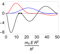
Figure 1: . Plot of expression from Eq. (Spin-momentum locking and Majorana fermions in charge carrier hole epitaxial wires). Black- $m=-2$, red - $m=0$, blue - $m=1$. Here $\gamma_{1}=6.8$, $\gamma_{2}=2.1$, $\gamma_{3}=2.9$. Dots indicate the ground state and the first excited state

The ground state energy is obtained as the first solution of Eq. (Spin-momentum locking and Majorana fermions in charge carrier hole epitaxial wires) for $m=-2$ and $m=-1$. We denote $E_{0}=E_{0,-2}^{(0)}=E_{0,-1}^{(0)}$ for $m=-2$ and $m=-1$ . The second solution of Eq. (Spin-momentum locking and Majorana fermions in charge carrier hole epitaxial wires)is the first excited state. The wavefunctions of the double-degenerate ground state are given by

$$\Psi_{0,-2}^{0} = {\mathcal{N}}\left(\begin{array}[]{c}\frac{\Gamma-2\gamma_{2}}{\sqrt{3}\left(\gamma_{2}+\gamma_{3}\right)}F_{2}(k_{1},k_{2},R,r)e^{-2i\phi}\\ 0\\ F_{0}(k_{1},k_{2},R,r)\\ 0\end{array}\!\right),$$ (15)

$$\Psi_{0,-1}^{0} = {\mathcal{N}}\left(\begin{array}[]{c}0\\ F_{0}(k_{1},k_{2},R,r)\\ 0\\ \frac{\Gamma-2\gamma_{2}}{\sqrt{3}\left(\gamma_{2}+\gamma_{3}\right)}F_{2}(k_{1},k_{2},R,r)e^{2i\phi}\end{array}\right),$$ (20)

where $k_{i}={\mathcal{K}}_{i}(E_{0})$, $\mathcal{N}$ is the normalization factor and

$$F_{n}(k_{1},k_{2},R,r)=J_{n}\left(k_{1}r\right)-\frac{J_{n}\left(k_{1}R\right)}{J_{n}\left(k_{2}R\right)}J_{n}\left(k_{2}r\right)$$ (21)

The dominant component in these wavefunctions corresponds to the angular momentum $\pm 1/2$.

The first order in $k_{z}$, the expansion does not lead to any corrections to energy, as it should be on symmetry grounds in the absence of the linear in hole momentum spin-orbit interactions; $E_{n,m}^{(1)}=0$. However corrections to the ground state wavefunctions are non-zero and are given by

$$\Psi_{0,-2}^{1} = +iF_{1}(k_{1},k_{2},R,r)\left(\begin{array}[]{c}0\\ \delta_{1}e^{-i\phi}\\ 0\\ \delta_{2}e^{i\phi}\end{array}\right)~{},$$ (26)

$$\Psi_{0,-1}^{1} = -iF_{1}(k_{1},k_{2},R,r)\left(\begin{array}[]{c}\delta_{2}e^{-i\phi}\\ 0\\ \delta_{1}e^{i\phi}\\ 0\end{array}\right)~{},$$ (31)

where

$$\delta_{1}\! \!=\! \frac{\gamma_{3}}{k_{1}}\frac{\Gamma-2\gamma_{2}}{\gamma_{2}+\gamma_{3}}\frac{4\gamma_{1}+2\Gamma}{4\gamma_{1}\gamma_{2}-\Gamma^{2}}\left[1-\frac{k_{2}J_{1}\left(k_{1}R\right)J_{2}\left(k_{2}R\right)}{k_{1}J_{1}\left(k_{2}R\right)J_{2}\left(k_{1}R\right)}\right]$$

$$\delta_{2}\! \!=\! \frac{4}{\sqrt{3}}\frac{\Gamma-2\gamma_{2}}{\left(\gamma_{2}+\gamma_{3}\right)^{2}k_{1}}-\frac{1}{\sqrt{3}}\frac{\Gamma-2\gamma_{2}}{\gamma_{2}+\gamma_{3}}\delta_{1}$$ (33)

Thus the two degenerate ground state wavefunctions are given by

$$\Psi_{0,-2,k_{z}}\approx\Psi_{0,-2}^{0}+k_{z}\Psi_{0,-2}^{1}~{},$$ (34)

$$\Psi_{0,-1,k_{z}}\approx\Psi_{0,-1}^{0}+k_{z}\Psi_{0,-1}^{1}~{}.$$ (35)

The expansion of Eqs. (3) and (5) up to $k_{z}^{2}$ terms defines the effective mass of holes. A tedious but straightforward calculation gives the coefficient in front of $k^{2}_{z}$, $E_{n,m}^{(2)}$. The effective mass for motion along the wire is $1/2E_{n,m}^{(2)}$, $(\hbar=1)$. Its analytic expression is rather complicated but a simplified one can be written for $\gamma_{2}=\gamma_{3}$. Using the notations $\nu=(\gamma_{1}+2\gamma_{2})/(\gamma_{1}-2\gamma_{2})$ and $\tilde{f}_{n}^{m}=J_{n}(k_{1})J_{m}(k_{1}\sqrt{\nu})$, we obtain

$$m=\left[\nu k_{1}\tilde{f}_{1}^{1}\left(-3\tilde{f}_{1}^{0}+\tilde{f}_{1}^{2}-\sqrt{\nu}\tilde{f}_{0}^{1}+3\sqrt{\nu}\tilde{f}_{2}^{1}\right)\right]^{-1}$$

$$\left[6(\nu-1)\tilde{f}_{2}^{0}f_{1}^{1}+\left(-3\sqrt{\nu}\tilde{f}_{1}^{0}+\sqrt{\nu}\tilde{f}_{1}^{2}-\tilde{f}_{0}^{1}+3\tilde{f}_{2}^{1}\right)\right.$$

$$\times\sqrt{\nu}k_{1}\tilde{f}_{1}^{1}-\left.6\left(\sqrt{\nu}\tilde{f}_{1}^{0}\tilde{f}_{1}^{2}-(\nu+1)\tilde{f}_{2}^{0}\tilde{f}_{1}^{1}+\sqrt{\nu}\tilde{f}_{0}^{1}\tilde{f}_{2}^{1}\right)\right]$$ (36)

The analysis of this expression shows that the effective mass can be infinite, so that there are no $k_{z}^{2}$ terms in the energy spectrum. In Fig. 2 we plot the inverse effective mass as a function of the ratio of the bulk light and heavy hole masses $\nu$ and anisotropy coefficient $\delta=(\gamma_{3}-\gamma_{2})/(\gamma_{3}+\gamma_{2})$. The black line corresponds to the infinite mass. In the dark blue region the mass is very small due to the crossing of the ground state and the first excited level. We have calculated the effective masses for wires made of the several semiconductor compounds.

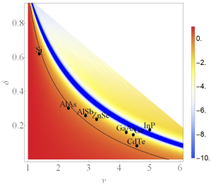
Figure 2: Inverse effective mass as a function of the ratio of heavy and light bulk hole masses $\nu$ and anisotropy parameter $\delta$. Black line corresponds to $1/m_{eff}=0$, while the dark blue region indicates a very small mass, due to crossing between the ground state and the first excited state.

When the mass is infinite (or, in other terms, the inverse mass vanishes or is close to zero), the leading terms in the spectrum of holes are linear in momentum and spin terms. These terms can emerge due to asymmetry of the confining potential of the wire or due to the bulk inversion asymmetry. We now consider asymmetry of the confining potential, which can be described by the presence of the electric field. The effect of an electric field $\bm{\mathcal{E}}$ that is perpendicular to the wire axis is described by Hamiltonian

$$H_{e}=e\mathcal{E}r\cos(\phi-\phi_{0})~{},$$ (37)

where $\phi_{0}$ is the angle between $\bm{\mathcal{E}}$ and the $x$-axis.The matrix elements of $H_{e}$ on the two degenerate wavefunctions of the ground state (expanded up to first order in $k_{z}$) are given by

$$\braket{\psi_{0,-2,k_{z}}\left missing}{H_{e}}{\psi_{0,-2,k_{z}}} = \braket{\psi_{0,-1,k_{z}}\left missing}{H_{e}}{\psi_{0,-1,k_{z}}}=0$$

$$\braket{\psi_{0,-2,k_{z}}\left missing}{H_{e}}{\psi_{0,-1,k_{z}}} = -ik_{z}\beta\mathcal{E}\exp(i\phi_{0})~{},$$ (38)

where $\beta$ is evaluated using Eqs. (15-31). In addition to $H_{e}$, the electric field in the presence of mixing of higher bands in III-V or Ge and Si semiconductors leads to a standard spin-orbit Hamiltonian for bulk holes

$$H_{R}=\beta_{R}\mathcal{E}\left(J_{x}\cos\phi_{0}-J_{y}\sin\phi_{0}\right)k_{z}$$ (39)

where $\beta_{R}$ is the Rashba coefficient characterizing bulk interaction (39) Liang and Lyanda-Geller (2017). The matrix elements of this Hamiltonian between degenerate ground states of Eqs. (15) and (20) are given by

$$\braket{\psi_{0,-2,k_{z}}\left missing}{H_{R}}{\psi_{0,-2,k_{z}}} = \braket{\psi_{0,-1,k_{z}}\left missing}{H_{R}}{\psi_{0,-1,k_{z}}}=0$$

$$\braket{\psi_{0,-2,k_{z}}\left missing}{H_{e}}{\psi_{0,-1,k_{z}}} = \beta_{R}{\mathcal{E}}{\mathcal{M}}e^{-i\phi_{0}}k_{z}$$ (40)

where

$${\mathcal{M}}={\mathcal{N}}^{2}\int_{0}^{R}{drr}{\left[J_{0}\left(k_{1}r\right)-\frac{J_{0}\left(k_{1}R\right)}{J_{0}\left(k_{2}R\right)}J_{0}\left(k_{2}r\right)\right]^{2}}.$$ (41)

In the Hilbert space of the two degenerate ground state wavefunctions $\psi_{0,-1,k_{z}}$ and $\psi_{0,-2,k_{z}}$, $H_{e}+H_{R}$ acts as an effective Rashba and Zeeman Hamiltonian

$$H_{eff}^{RZ}=\beta k_{z}\bm{\mathcal{E}}\times\bm{\sigma}+\beta_{R}\mathcal{M}k_{z}\bm{\mathcal{E}}\cdot\bm{\sigma}~{}.$$ (42)

When the inverse mass vanishes, matrix element $\mathcal{M}$ is very close to unity while coefficient $\beta$ depends on the radius of the wire and is plotted in Fig. 3

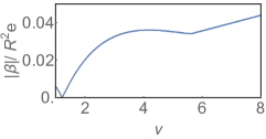
Figure 3: Coefficient $\beta$ at the points of infnite mass

The wire Hamiltonian is similar to Hamiltonian describing an edge in topological insulators Fu and Kane (2008); Alicea (2012),

$${\cal H}_{w}=\int dz\Psi^{\dagger}\left(-iv\partial_{z}-\mu\right)\Psi,$$ (43)

where velocity $v$ is defined as

$$\hbar v=\mathcal{E}\sqrt{\beta_{R}^{2}\mathcal{M}^{2}+\beta^{2}+2\beta\beta_{R}\mathcal{M}\cos\left(2\phi_{0}\right)}$$ (44)

and $\Psi^{\dagger}_{z}$ adds an electron with spin $\sigma$ at a coordinate $z$. In the presence of superconducting proximity effect described by the induced order parameter $\Delta$, which couples charge carriers with opposite spins, given by

$${\cal H}_{\Delta}=\int dz\Delta\left(\Psi_{\downarrow}\Psi_{\uparrow}+H.C\right),$$ (45)

the Bogoliubov-DeGennes Hamiltonian ${\cal H}_{BdG}={\cal H}_{w}+{\cal H}_{\Delta}$ leads to quasiparticle energies

$$E_{\pm}(k)=\sqrt{(\pm vk-\mu)^{2})+\Delta^{2}},$$ (46)

describing a gapped topological superconductor. In contrast to conventional semiconducting wires with shifted parabolic Rashba/Dresselhaus spectrum, where topological superconductivity and Majorana fermions at the end of the wire arise at Zeeman splitting of order to superconducting gap, here they emerge even at zero magnetic field. In a finite magnetic field $\mathbf{H}$ , e.g., along $z-axis$, the quasiparticle energies are given by

$$E_{\pm}(k)=\sqrt{\frac{\epsilon_{+}^{2}+\epsilon_{-}^{2}}{2}\pm\left(\epsilon_{+}-\epsilon_{-}\right)\sqrt{\Delta_{s}^{2}+\mu^{2}}+\Delta^{2}},$$ (47)

where $\epsilon_{\pm}=-\mu\pm\sqrt{(vk)^{2}+Z^{2}}$, $Z=g\mu_{B}H$ is the Zeeman energy, $\mu_{B}$ is the Bohr magneton and $g$ is the longitudinal $g-$factor along the direction of the wire, $\Delta_{s}=Z\Delta/\sqrt{(vk)^{2}+Z^{2}}$ is the strength of induced s-paring in the wire. Notably, $\Delta_{s}$ is nonzero only in the presence of magnetic field. The quasiparticle gap vanishes at magnetic field corresponding to $Z=\Delta^{2}+\mu^{2}$. At a higher magnetic fields the gap reopens, but the the superconductivity is no longer topological, while at a smaller fields the superconductivity is topological. If the proximity pairing amplitude $\Delta$ varies along the wire, then at a certain magnetic field, the topological superconductor will be in the region of the wire with $\Delta>Z$, while the conventional superconductor will be in the region with $\Delta<Z$. Tuning $Z$ can make possible moving the Majorana zero modes, localized at the boundaries between topological and non-topological regions. In the Rashba wires with parabolic spectrum, the situation is the opposite: the topological superconductivity persists at the Zeeman energy larger than $\Delta^{2}+\mu^{2}$.

It is known that parameters of the valence band, such as masses can be tuned not only varying the composition of heterostructure materials, but also tuning external parameters, e.g. such as strain. This potentially opens a possibility to induce an infinite mass in the wire by strain, and to observe transition between the cases of Rashba wire and spin-locked wire.

I Acknowledgement

This work is supported by the U.S. Department of Energy, Office of Basic Energy Sciences, Division of Materials Sciences and Engineering under Award DE-SC0010544.

References

• Nedorezov (1971) S. Nedorezov, Sov. Phys. Solid State 12, 1814 (1971).
• Merkulov et al. (1991) I. A. Merkulov, V. I. Perel, and M. E. Portnoi, Zh. Exper. Teor. Fiz 99, 1202 (1991).
• Rashba and Sherman (1988) E. Rashba and E. Y. Sherman, Physics Letters A 129, 175 (1988).
• Arovas and Lyanda-Geller (1998) D. P. Arovas and Y. B. Lyanda-Geller, Phys. Rev. B 57, 12302 (1998).
• Lyanda-Geller et al. (2004) Y. B. Lyanda-Geller, T. L. Reinecke, and M. Bayer, Phys. Rev B. 69, 161308 (2004).
• Bulaev and Loss (2005) D. V. Bulaev and D. Loss, Phys. Rev. Lett. 95, 076805 (2005).
• Bernevig and Zhang (2005) B. A. Bernevig and S.-C. Zhang, Phys. Rev. Lett. 95, 016801 (2005).
• Quay et al. (2010) C. H. L. Quay, T. Hughes, J. Sulpizion, L. Pfeiffer, K. Baldwin, K. West, D. Goldhaber-Gordon, and R. de Picciotto, Nature Physics 6, 336 (2010).
• Mao et al. (2012) L. Mao, M. Gong, E. Dumitrescu, S. Tewari, and C. Zhang, Phys. Rev. Lett. 108, 177001 (2012).
• Simion and Lyanda-Geller (2014) G. E. Simion and Y. B. Lyanda-Geller, Phys. Rev. B 90, 195410 (2014).
• Durnev et al. (2014) M. Durnev, M. Glazov, and E. Ivchenko, Phys. Rev. B 89, 075430 (2014).
• Liang and Lyanda-Geller (2017) J. Liang and Y. Lyanda-Geller, Phys. Rev. B 95, 201404 (2017).
• Kloeffel et al. (2011) C. Kloeffel, A. Trif, and D. Loss, Phys. Rev. B 84, 195314 (2011).
• Maier et al. (2014) F. Maier, J. Klinovaja, and D. Loss, Phys. Rev. B 90, 195421 (2014).
• Csontos et al. (2009) D. Csontos, P. Brusheim, U. Zülicke, and H. Xu, Phys. Rev. B 79, 155323 (2009).
• Fu and Kane (2008) L. Fu and C. L. Kane, Phys. Rev. Lett. 100, 096407 (2008).
• Alicea (2012) J. Alicea, Reports on Progress in Physics 75, 076501 (2012).
• Lutchyn et al. (2010) R. M. Lutchyn, J. D. Sau, and S. Das Sarma, Phys. Rev. Lett. 105, 077001 (2010).
• Oreg et al. (2010) Y. Oreg, G. Refael, and F. von Oppen, Phys. Rev. Lett. 105, 177002 (2010).