ThumbNet: One Thumbnail Image Contains All You Need for Recognition

Abstract.

Although deep convolutional neural networks (CNNs) have achieved great success in computer vision tasks, its real-world application is still impeded by its voracious demand of computational resources. Current works mostly seek to compress the network by reducing its parameters or parameter-incurred computation, neglecting the influence of the input image on the system complexity. Based on the fact that input images of a CNN contain substantial redundancy, in this paper, we propose a unified framework, dubbed as ThumbNet, to simultaneously accelerate and compress CNN models by enabling them to infer on one thumbnail image. We provide three effective strategies to train ThumbNet. In doing so, ThumbNet learns an inference network that performs equally well on small images as the original-input network on large images. With ThumbNet, not only do we obtain the thumbnail-input inference network that can drastically reduce computation and memory requirements, but also we obtain an image downscaler that can generate thumbnail images for generic classification tasks. Extensive experiments show the effectiveness of ThumbNet, and demonstrate that the thumbnail-input inference network learned by ThumbNet can adequately retain the accuracy of the original-input network even when the input images are downscaled 16 times.

1. Introduction

Recent years have witnessed not only the growing performance of deep convolutional neural networks (CNNs) (Simonyan and Zisserman, 2015; He et al., 2016; Xie et al., 2017; Zhao et al., 2018a; Xu et al., 2020; Zhao et al., 2017b, 2018b), but also their expanding computation and memory costs (Canziani et al., 2016). Though the intensive computation and gigantic resource requirements are somewhat tolerable in the training phase thanks to the powerful hardware accelerators (e.g. GPUs), when deployed in real-world systems, a deep model can easily exceed the computing limit of hardware devices. Mobile phones and tablets, which have constrained power supply and computational capability, are almost intractable to run deep networks in real-time. A cloud service system, which needs to respond to thousands of users, has an even more stringent requirement of computing latency and memory. Therefore, it is of practical significance to accelerate and compress CNNs for test-time deployment.

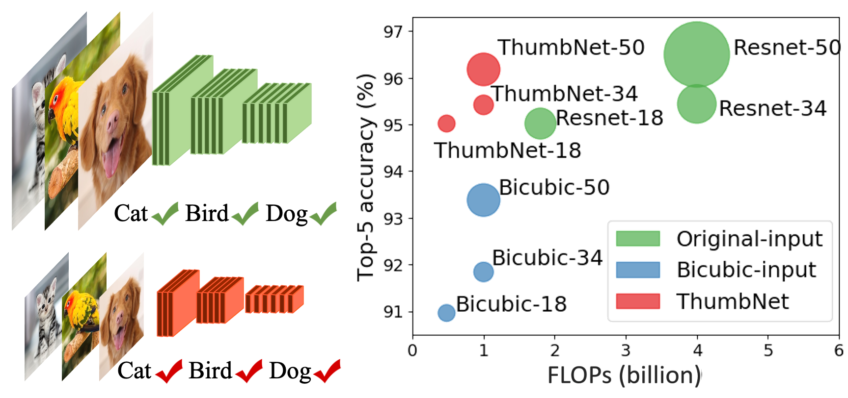
Figure 1. Same CNN with different input sizes. We accelerate a CNN by inferring on thumbnail images. Compared to the original-input network shown on the top-left, the thumbnail-input CNN shown on the bottom-left has the same architecture but smaller feature maps in all convolutional layers, hereby tremendously reducing computation and memory requirements, as shown on the right (circle sizes indicate memory requirements). The proposed ThumbNet can well retain the accuracy of the original-input networks, significantly outperforming the bicubic-input networks that input small images downscaled via bicubic interpolation.

Before delving into the question of how to speed up deep networks, let us first analyze what dominates the computational complexity of a CNN. We calculate the total time complexity of convolutional layers as follows (He and Sun, 2015):

(1) $$\mathcal{O}\left(\sum\nolimits_{l=1}^{d}n_{l-1}\cdot s^{2}_{l}\cdot n_{l}\cdot m^{2}_{l}\right),$$

where $l$ is the index of a layer and $d$ is the total number of layers; $n_{l-1}$ is the number of input channels and $n_{l}$ is the number of filters in the $l$-th layer; $s_{l}^{2}$ is the spatial size of the filters and $m_{l}^{2}$ is the spatial size of the output feature map.

Decreasing any factor in Eq. (1) can lead to reduction of total computation. One way is to sparsify network parameters by filter pruning (LeCun et al., 1990; Han et al., 2016), which by defining some mechanism to prioritize the parameters, sets unimportant ones to zero. However, some researchers claim that these methods usually require sparse BLAS libraries or even specialized hardware. Hereby, they propose to prune filters as a whole (Li et al., 2016; Luo et al., 2017). Another method is to decrease the number of filters by low rank factorization (Denton et al., 2014; Jaderberg et al., 2014; Lebedev et al., 2014; Zhang et al., 2016). If a more dramatic change in network structure is required, knowledge distillation (Hinton et al., 2015; Romero et al., 2014) can do the trick. It generates a new network, which can be narrower (with fewer filters) or shallower (with fewer layers), by transferring hidden information from the original network. Moreover, there are other approaches to lower the convolution overload by means of fast convolution techniques (e.g. FFT (Mathieu et al., 2013) and the Winograd algorithm (Lavin and Gray, 2016)), and quantization (Han et al., 2016; Wu et al., 2016) and binarization (Courbariaux et al., 2016; Rastegari et al., 2016).

All the above methods attempt to accelerate or compress neural networks from the viewpoint of network parameters, thereby neglecting the significant role that the spatial size of feature maps are playing in the overall complexity. According to Eq. (1), the required computation is diminished as the spatial size of feature maps decreases. Moreover, the memory required to accommodate those feature maps at run-time will also be reduced. Given a CNN architecture, we can simply decrease the spatial size of all feature maps by reducing the size of the input image.

In this paper, we propose to use a thumbnail image, i.e., an image of lower spatial resolution than its original-size counterpart, as test-time network input to accelerate and compress CNNs of any architecture and of any depth and width. This thumbnail-input network can dramatically reduce computation as well as memory requirements, as shown in Fig. 1.

Contributions. (1) We propose an orthogonal mechanism to accelerate a deep network compared to conventional methods: from the novel perspective of enabling the network to infer on one single downscaled image efficiently and effectively. To this end, we propose a unified framework called ThumbNet to train a thumbnail-input network that can tremendously reduce computation and memory consumption while maintaining the accuracy of the original-input network. (2) We present a supervised image downscaler that generates a thumbnail image with good discriminative properties and a natural chromatic look. This downscaler is reliably trained by exploiting supervised image downscaling, distillation-boosted supervision, and feature-mapping regularization. The ThumbNet generated images can replace their original-size counterparts and be stored for other classification-related tasks, reducing resource requirements in the long run. (3) The proposed ThumbNet effectively preserves network accuracy at speedup ratios of up to $4\times$ (Imagenet) and $16\times$ (Places) on various networks, surpassing other network acceleration/compression methods by significant margins.

2. Related Work

In this section, we give an overview of the related works to our proposed ThumbNet in the literature.

2.1. Knowledge Distillation

Knowledge Distillation (KD) (Hinton et al., 2015) was introduced as a model compression framework, which aims to reduce the computational complexity of a deep neural network by transferring knowledge from its original architecture (teacher) to a smaller one (student). The student is penalized according to the discrepancy between the softened versions of the teacher’s and student’s output logits. It claims that this teacher-student paradigm easily transfers the generalization capability of the teacher network to the student network in that the student not only learns the characteristics of the correct labels but can also benefit from the invisible finer structure in the wrong labels. There are some extensions to this work, e.g., using intermediate representations as hints to train a thin-and-deep student network (Romero et al., 2014), applying it in object detection models (Chen et al., 2017), and using it to enhance network resilience to adversarial samples (Papernot et al., 2016). These works mostly focus on learning a new network architecture. In our paper, we utilize the idea of KD to train the same network architecture with thumbnail images as input.

2.2. Auto-Encoder

An auto-encoder (Hinton and Salakhutdinov, 2006) is an unsupervised neural network, which learns a data representation of reduced dimensions by minimizing the difference between input and output. It consists of two parts, an encoder which maps the input to a latent feature, and a decoder which reconstructs the input from the latent feature. Early auto-encoders are mostly composed of fully-connected layers (Hinton and Salakhutdinov, 2006; Bourlard and Kamp, 1988). These days, with the popularity of CNNs, some researchers propose to incorporate convolution to an auto-encoder and design a convolutional auto-encoder (Turchenko et al., 2017; Masci et al., 2011), which utilizes convolution / pooling to downscale the image in the encoder and utilizes deconvolution (Zeiler et al., 2010) / unpooling in the decoder to restore the original image size. Though the downscaled images from the encoder are effective for reconstructing the original images, they do not perform well for classification due to lack of supervision. In our work, instead of using convolutional auto-encoder as a downscaler, we incorporate it into ThumbNet as unsupervised pre-training to regularize the classification task.

2.3. Downscaled Image Representation

Representing an image with a downscaled size is an effective way to reduce computational complexity. One emerging method is to apply compressive sensing (Zhao et al., 2017b, 2018b; Zhang et al., 2012, 2014; Zhao et al., 2017a, 2016; Zhao et al., 2014) when acquiring an image to sample only a small number of measurements. But these measurements are not in the format of 2D grid and cannot be directly processed by a CNN. Alternatively, the work WIDIC (Zhao et al., 2013) proposes to downscale an image into a smaller image in the wavelet domain, so as to increase its coding efficiency without compromising reconstruction quality. The proposed ThumbNet also preserves the image grid when downscaling but in a learnable manner. It focuses on the classification task and aims to increase network efficiency instead. For the task of classification, we find one recent work (Chen et al., 2018) (denoted here as LWAE), which also attempts to accelerate a neural network by using small images as input. It decomposes the original input image into two low-resolution sub-images, one with low frequency which is fed into a standard classification network, and one with high frequency which is fused with features from the low-frequency channel by a lightweight network to obtain the classification results. Compared to LWAE, our ThumbNet is able to achieve higher network accuracy with one single thumbnail-image, resulting in fewer requirements for computation, memory and storage.

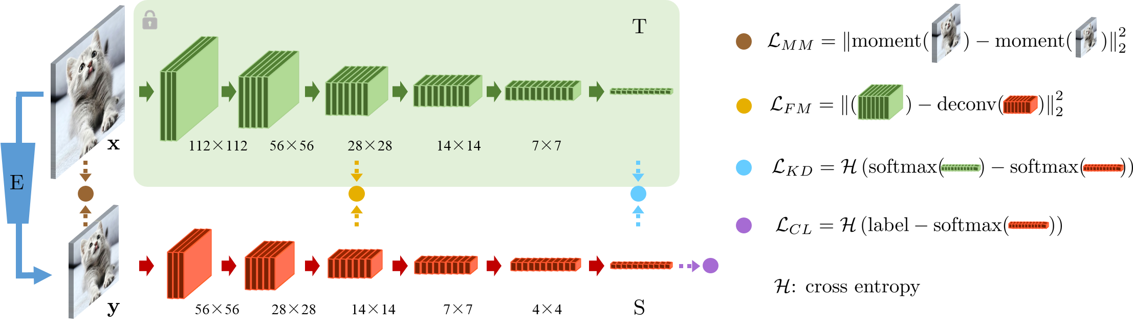
Figure 2. ThumbNet Architecture. Green: well-trained network $\mathrm{T}$; red: inference network $\mathrm{S}$; blue: downscaler $\mathrm{E}$. Blocks represent feature maps, solid arrows contain network operations such as convolution, the rectified linear unit (ReLU) (Nair and Hinton, 2010), pooling, batch normalization (Ioffe and Szegedy, 2015), etc. The numbers below each feature map are their spatial resolutions. Dots represent the four losses, which are moment-matching (MM) loss in brown, feature-mapping (FM) loss in yellow, knowledge-distillation (KD) loss in cyan and classification (CL) loss in purple.

3. Proposed ThumbNet

3.1. Network Architecture

We illustrate the architecture of ThumbNet in Fig. 2. The well-trained network $\mathrm{T}$ takes an input image of a large size, e.g., $224\times 224$, passes it through stacked convolutional layers and fully-connected layers, and produces $K$ logits, where $K$ is the number of classes. Its well-trained parameters $\mathbf{W}_{\mathrm{T}}$, are not changed during the whole training process of ThumbNet and only provide guidance for the inference network. The inference network $\mathrm{S}$, which takes as input an image of a small size, e.g., $112\times 112$. Each layer of $\mathrm{S}$ (except for the first fully-connected layer if its size is influenced by the input image size as in VGG), has exactly the same shape and size as its corresponding layer in $\mathrm{T}$. Each feature map of $\mathrm{S}$ has the same number of channels as its corresponding feature map of $\mathrm{T}$ but is smaller in the spatial size. The parameters in $\mathrm{S}$, denoted as $\mathbf{W}_{\mathrm{S}}$, are the main learning objectives of ThumbNet. The downscaler $\mathrm{E}$ generates a thumbnail image from the original input image, whose parameters are denoted as $\mathbf{W}_{\mathrm{E}}$.

3.2. Details of Network Design

There are three main techniques in the proposed ThumbNet: 1) supervised image downscaling, 2) distillation-boosted supervision, and 3) feature-mapping regularization.

3.2.1. Supervised Image Downscaling

Traditional image downscaling methods (e.g., bilinear and bicubic (Lehmann et al., 1999)) do not consider the discriminative capability of the downscaled images, which as a consequence lose critical information for classification. We instead exploit CNNs to adaptively extract discriminative information from the original images to tailor to the classification goal.

Algorithm 1 Training Strategy of ThumbNet
The well trained parameters $\mathbf{W}_{\mathrm{T}}$ of the original network are provided as input to the algorithm. All the trainable parameters are initialized as random values which are denoted by $\mathbf{W}_{\mathrm{S}}^{0}$, $\mathbf{W}_{\mathrm{E}}^{0}$, $\mathbf{W}_{\mathrm{D}}^{0}$.

1:Input: $\mathbf{W}_{\mathrm{T}}$, $\mathbf{W}_{\mathrm{S}}^{0}$, $\mathbf{W}_{\mathrm{E}}^{0}$, $\mathbf{W}_{\mathrm{D}}^{0}$

2:$\mathbf{W}_{\mathrm{E}}^{\ast},\mathbf{W}^{\ast}_{\mathrm{S}_{l}},\mathbf{W}^{\ast}_{\mathrm{D}}\;\leftarrow\underset{\mathbf{W}_{\mathrm{E}},\mathbf{W}_{\mathrm{S}_{l}},\mathbf{W}_{\mathrm{D}}}{\operatorname{arg\,min}}\mathcal{L}_{MM}\left(\mathbf{W}_{\mathrm{E}}\right)+\alpha\mathcal{L}_{FM}\left(\mathbf{W}_{\mathrm{E}},\mathbf{W}_{\mathrm{S}_{l}},\mathbf{W}_{\mathrm{D}}\right)+\frac{1}{2}\theta\mathcal{R}_{\mathrm{E},\mathrm{S}_{l},\mathrm{D}}$

3:$\mathbf{W}_{\mathrm{E}}^{\ast},\mathbf{W}_{\mathrm{S}}^{\ast}\;\leftarrow\underset{\mathbf{W}_{\mathrm{E}},\mathbf{W}_{\mathrm{S}}}{\operatorname{arg\,min}}\;\mathcal{L}_{CL}\left(\mathbf{W}_{\mathrm{E}},\mathbf{W}_{\mathrm{S}}\right)+\beta\mathcal{L}_{KD}\left(\mathbf{W}_{\mathrm{E}},\mathbf{W}_{\mathrm{S}}\right)+\frac{1}{2}\theta\mathcal{R}_{\mathrm{E},\mathrm{S}}$

4:Output: $\mathbf{W}_{\mathrm{E}}^{\ast}$, $\mathbf{W}_{\mathrm{S}}^{\ast}$

For the sake of computational efficiency and simplicity, our supervised image downscaler $\mathrm{E}$ merely comprises two convolutional layers, each with a $5\times 5$ convolutional operation followed by batch normalization and the rectified linear unit (ReLU). In the first layer, there are more output channels than input channels to empower the network to learn more intermediate features, and in the second layer there are exactly 3 output channels to restore the image color channel. The stride of each layer depends on the required downscaling ratio. Compared to bicubic, this learnable downscaler not only adaptively trains the filters, but also incorporates non-linear operations and high-dimensional feature projection. By denoting all the nested operations in our downscaler as $\mathcal{E}$, we obtain a small image $\mathbf{y}$ from the original image $\mathbf{x}$ via the following:

(2) $$\mathbf{y}=\mathcal{E}\left(\mathbf{x};\mathbf{W}_{\mathrm{E}}\right).$$

A significant consideration in designing this downscaler is that the generated small image should remain visually pleasant and recognizable, e.g., the information in the color channels should not be destroyed or misaligned. That is to say, if pixel values in natural images follow a distribution, then the generated small image should follow the same distribution with similar moments. Hereby, we propose a moment-matching (MM) loss as follows:

(3) $$\mathcal{L}_{MM}\left(\mathbf{W}_{\mathrm{E}}\right)=\frac{1}{3}\left\|\mathcal{\mu}\left(\mathbf{x}\right)-\mathcal{\mu}\left(\mathbf{y}\right)\right\|^{2}_{2}+\lambda\frac{1}{3}\left\|\mathcal{\sigma}\left(\mathbf{x}\right)-\mathcal{\sigma}\left(\mathbf{y}\right)\right\|_{2}^{2},$$

where $\mathcal{\mu}(\cdot)$ and $\mathcal{\sigma}(\cdot)$ compute the first and second moments respectively of the image pixel values in each color channel, and $\lambda$ is a tunable parameter that balances the two moments. This MM loss encourages that the mean and variance (loosely approximating the distribution) in each color channel of the downscaled image stay close to the mean and variance of the original image. This has been used in other application as well in the literature, such as deep generative model learning (Li et al., 2015) and style transfer (Li et al., 2017).

Please note that this downscaler is not trained independently with merely the MM loss, but incorporated into the whole architecture of ThumbNet and trained together with other components and losses. This includes the classification loss, which provides supervision to the image downscaling process, guiding it to generate a small image that is discriminative for accurate classification. Hence, we name $\mathrm{E}$ a supervised image downscaler. Once trained, this downscaler can be used for generating small images, which are not only used as input of the inference network, but also for other classification-related tasks as well.

3.2.2. Distillation-Boosted Supervision

A straightforward way to train the network is to minimize the classification (CL) loss defined as follows:

(4) $$\mathcal{L}_{CL}\left(\mathbf{W}_{\mathrm{E}},\mathbf{W}_{\mathrm{S}}\right)=\mathcal{H}\left(\mathbf{b},\,\mathcal{S}\left(\mathbf{y};\mathbf{W}_{\mathrm{S}}\right)\right),$$

where $\mathbf{y}$ is calculated as in Eq. (2), $\mathbf{b}$ indicates the ground-truth labels, $\mathcal{S}\left(\cdot\right)$ denotes all the nested functions in the inference network $\mathrm{S}$, and $\mathcal{H}$ refers to cross entropy. This loss seeks to match the predicted label with the ground-truth label and is a typical cost function for supervised learning. However, only using this loss cannot exploit the information embedded in the well-trained model $\mathrm{T}$. To address this issue, we propose to distill the learned knowledge in $\mathrm{T}$ and transfer it to the inference network. Therefore, apart from the CL loss, we also enforce the computed probabilities of each class in the inference network to match those in the well-trained network.

Let $\mathcal{S}_{0}\left(\cdot\right)$ and $\mathcal{T}_{0}\left(\cdot\right)$ denote the deep nested functions before softmax in the inference network and the well-trained network, respectively. Then, their logits are calculated as:

(5) $$\mathbf{a}_{\mathrm{S}}=\mathcal{S}_{0}\left(\mathbf{y};\mathbf{W}_{\mathrm{S}}\right),\;\mathbf{a}_{\mathrm{T}}=\mathcal{T}_{0}\left(\mathbf{x}\right).$$

Following (Hinton et al., 2015), we define the knowledge-distillation (KD) loss as the cross entropy between the two softened probabilities:

(6) $$\mathcal{L}_{KD}\left(\mathbf{W}_{\mathrm{E}},\mathbf{W}_{\mathrm{S}}\right)=\mathcal{H}\left(\textrm{softmax}\left(\frac{\mathbf{a}_{S}}{\tau}\right),\,\textrm{softmax}\left(\frac{\mathbf{a}_{T}}{\tau}\right)\right),$$

where $\tau$ is the temperature to soften the class probabilities and is usually greater than 1. With the aid of this KD loss, the supervised training process of ThumbNet can benefit from the well-trained model to learn finer discriminative structures, so we call it distillation-boosted supervision.

3.2.3. Feature-Mapping Regularization

It is widely observed that unsupervised pre-training, e.g., using an auto-encoder, can help with supervised learning tasks as a form of regularization (Erhan et al., 2010). Inspired by this, we design the feature-mapping (FM) regularization to pre-train ThumbNet.

In Fig. 2, ThumbNet is partitioned into two segments by the FM loss (the yellow dot). In order to give a clearer sense of the rationale, we re-illustrate the left segment of ThumbNet along with the FM loss from a different point of view in Fig. 3 (note that the MM loss is left out and the deconvolution in the FM loss is unrolled for the sake of clarity). We can see that it is analogous to an auto-encoder, which is trained by minimizing the difference between the pre-processed input and the output.

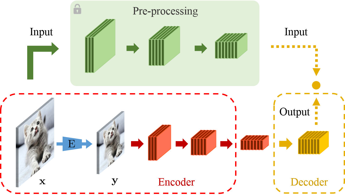
Figure 3. Feature-mapping regularization. This re-illustrates the left segment of ThumbNet along with the FM loss, which is essentially an auto-encoder. The layers in the red dashed box constitute the encoder, the layers in the yellow dashed box constitute the decoder, and the feature map in the middle is learned latent representation. The shaded area can be viewed as a pre-processing for the input. The yellow solid arrow represents deconvolutional layers and the yellow block is the upscaled feature map.

In the decoder, each deconvolutional layer has a stride size 2 and the number of layers is determined by the downscaling ratio. The decoder does not change the number of channels but upscales the feature map in $\mathrm{S}$ to match the spatial size of the corresponding feature map in $\mathrm{T}$. We compute their mean square error as the FM loss:

(7) $$\mathcal{L}_{FM}\left(\mathbf{W}_{\mathrm{E}},\mathbf{W}_{\mathrm{S}_{l}},\mathbf{W}_{\mathrm{D}}\right)=\frac{1}{2N}\left\|\mathcal{T}_{l}\left(\mathbf{x}\right)-\mathcal{D}\left(\mathcal{S}_{l}\left(\mathbf{y};\mathbf{W}_{\mathrm{S}_{l}}\right);\mathbf{W}_{\mathrm{D}}\right)\right\|_{2}^{2},$$

where $N$ is the product of all dimensions of the intermediate feature map in $\mathrm{T}$. $\mathcal{T}_{l}$ represents the nested functions in the left segment of the original network, $\mathcal{S}_{l}$ represents the nested functions in the left segment of the inference network, $\mathcal{D}$ represents operations in the deconvolutional layers, and $\mathbf{W}_{\mathrm{S}_{l}}$ and $\mathbf{W}_{\mathrm{D}}$ refer to the parameters in the left segment of $\mathrm{S}$ and in the deconvolutional layers, respectively.

3.3. Training Details

We summarize the training strategy of ThumbNet in Algorithm 1. In Algorithm 1, the $\mathcal{R}$ terms refer to ${l}_{2}$ regularization of the corresponding parameters, and $\theta,\alpha,\beta$ are the tradeoff weights. In Line 2, we perform an unsupervised pre-training by minimizing the MM loss and the FM loss, and obtain the parameters $\mathbf{W}^{\ast}_{\mathrm{E}}$ and $\mathbf{W}^{\ast}_{\mathrm{S}_{l}}$. In Line 3, we perform the distillation-boosted supervised learning by minimizing the KD loss and CL loss, using the values $\mathbf{W}^{\ast}_{\mathrm{E}}$ and $\mathbf{W}^{\ast}_{\mathrm{S}_{l}}$ as initialization for the corresponding parameters. In this step, we train the whole ThumbNet end-to-end to learn the optimal values for the parameters $\mathbf{W}^{\ast}_{\mathrm{E}}$ and $\mathbf{W}^{\ast}_{\mathrm{S}}$. Note that the parameters $\mathbf{W}^{\ast}_{\mathrm{E}}$ and $\mathbf{W}^{\ast}_{\mathrm{S}_{l}}$ are already pre-trained via Line 2, so they are only finetuned with a small learning rate. In contrast, we use a relatively large learning rate for the untrained parameters $\mathbf{W}_{\mathrm{S}_{r}}$ in the right segment.

We set the hyper-parameters in ThumbNet as follows. We use a starting learning rate 0.1, and divide it by 10 when the loss plateaus. We use a momentum 0.9 for the optimizer and the weight decay $\theta$ is $0.0001$. The parameters $\alpha$ and $\beta$ in Algorithm 1 are 1.0 and 0.5, respectively; $\tau$ in Eq. (6) is 2; $\lambda$ in Eq. (3) is 0.1. For finetuning the pre-trained parameters $\mathbf{W}_{\mathrm{E}}$ and $\mathbf{W}_{\mathrm{S}_{l}}$, the learning rate is set to $0.01$ times that of the other parameters, meaning their learning rate starts from $0.001$ and is decreased by 10 in the same fashion.

4. Experiments

In this section, we demonstrate the performance of the inference network $\mathrm{S}$ obtained via ThumbNet in terms of classification accuracy and resource requirements. We also provide experiments to verify that the learned downscaler has generic applicability to other classification-related tasks as well.

4.1. Ablation Study

In order to study the effectiveness of the proposed techniques in ThumbNet, we ablate each technique individually and test the performance of the reduced version of ThumbNet. We provide experimental results on the object recognition and scene recognition tasks using different backbone networks (e.g., Resnet-50, VGG-11).

4.1.1. Baseline and Comparative Methods

Table 1. Configuration of different methods. (a) is the baseline, (b) does not use any of the three techniques, (c)-(e) contain one or two, and (f) consists of all of them.

Methods	SD	KD	FM
(a) Original / Direct	$-$	$-$	$-$
(b) Bicubic downscaler	×	×	×
(c) Supervised downscaler	✓	×	×
(d) Bicubic + distillation	×	✓	×
(e) Supervised + distillation	✓	✓	×
(f) ThumbNet	✓	✓	✓

We implement six variations of ThumbNet for training a backbone network, which are introduced in the following.

(a) Original / Direct. ‘Original’ refers to the network model trained on the original-size images. The testing performance of the model on an original-size image is the upperbound baseline for all the comparative methods. For networks like Resnet, which use global average pooling instead of fully-connected layers at the end, the ‘Original’ model can be directly used to test on a small image without altering the network structure. We refer to the case of directly using the ‘Original’ model for inference on small images without re-training as ‘Direct’, which is the lowerbound baseline for all the methods.

(b) Bicubic downscaler. This trains the network from scratch on images that are downscaled with the bicubic method.

(c) Supervised downscaler. This trains the network from scratch on small images that are downscaled with the supervised downscaler in ThumbNet. The downscaler and the network are trained jointly end-to-end based on the MM loss and the CL loss.

(d) Bicubic + distillation. This trains the network on bicubic-downscaled small images with the aid of distillation from the ‘Original’ model. The network is trained based on the KD loss and the CL loss.

(e) Supervised + distillation. This trains the network on supervised-downscaled small images with the aid of distillation from the ‘Original’ model. The supervised downscaler and the network are trained jointly end-to-end based on the MM loss, the KD loss and the CL loss.

(f) ThumbNet. This is the full configuration of our proposed method, which is trained on supervised-downscaled small images with the aid of distillation from the ‘Original’ models as well as feature mapping regularization. It is trained based on the four losses as described in Section 3.3.

In Table 1, we demonstrate the configuration of each method with respect to the three techniques used in ThumbNet: supervised image downscaling (SD), knowledge-distillation boosted supervision (KD) and feature mapping regularization (FM). The hyper-parameters in all the methods are the same, as specified in Section 3.3.

Table 2. Error rates (%) for scene recognition on Places36. ThumbNet retains the accuracy of the original-input network when downscaling the image 16 times.

	Resnet-18		VGG-11
Methods	Top-1	Top-5	Top-1	Top-5
(a) Original	21.11	3.28	19.75	3.61
(a) Direct	66.94	33.97	/	/
(b) Bicubic downscaler	32.08	7.83	27.83	10.17
(c) Supervised downscaler	25.94	5.31	24.28	6.58
(d) Bicubic+distillation	26.00	4.47	22.69	4.92
(e) Supervised+distillation	24.33	3.94	21.31	3.94
(f) ThumbNet	22.78	3.69	21.58	3.72

4.1.2. Object Recognition on ImageNet Dataset

We evaluate the performance of our proposed ThumbNet on the task of object recognition with the benchmark dataset ILSVRC 2012 (Deng et al., 2009), which consists of over one million training images drawn from 1000 categories. Besides using the full dataset (referred to as ImagenetFull), we also form a smaller new dataset by randomly selecting 100 categories from ILSVRC 2012 and refer to it as Imagenet100 (the categories in Imagenet100 are given in the supplementary material). With Imagenet100, we can efficiently compare all the methods on a variety of backbone networks. In addition, by partitioning ILSVRC 2012 into two parts (Imagenet100 and the rest 900 categories referred to as Imagenet900), we can also evaluate the downsampler on unseen data categories (see Section 4.3 for details). For backbone networks, we consider various architectures (ResNet (He et al., 2016) and VGG (Simonyan and Zisserman, 2015)) and various depths (from 11 layers to 50 layers).

In Table 3, we demonstrate the performance of all the methods with four different backbone networks in terms of top-1 and top-5 error rates on the validation data. The input image size of ‘Original’ is $224\times 224$ and the input image sizes of the other methods are $112\times 112$, meaning that in this experiment, the image downscaling ratio is $4:1$. Thus, compared to ‘Original’, our ThumbNet only uses $1/4$ computation and memory, which will be detailed in Section 4.1.4, and it also preserves the accuracy of the original models. ‘Direct’ is a baseline of inference on small images, compared to which our ThumbNet improves by large margins for all the different backbones. Moreover, by comparing different pairs of methods, we can obviously observe the contribution of each technique. By comparing (c) to (b) or comparing (e) to (d), we can see the benefits of supervised image downscaling. By comparing (e) to (c), we can see the benefits of distillation-boosted supervision. By comparing (f) to (e), we can see that the benefits of feature-mapping regularization. (f) ThumbNet always shows the lowest error rates.

Table 3. Error rates (%) for object recognition on Imagenet. By comparing (c) to (b) or comparing (e) to (d), we can see the benefits of supervised image downscaling. By comparing (e) to (c), we can see the benefits of distillation-boosted supervision. By comparing (f) to (e), we can see that the benefits of feature-mapping regularization. (f) ThumbNet always shows the lowest error rates.

	Imagenet100								ImagenetFull
	VGG-11		Resnet-18		Resnet-34		Resnet-50		Resnet-18		Resnet-34		Resnet-50
	Top-1	Top-5	Top-1	Top-5	Top-1	Top-5	Top-1	Top-5	Top-1	Top-5	Top-1	Top-5	Top-1	Top-5
(a) Original	13.64	4.36	17.54	4.98	15.06	4.56	12.72	3.50	29.71	10.46	26.19	8.55	23.59	6.90
(a) Direct	/	/	37.26	16.94	34.48	14.32	29.42	11.80	50.74	26.15	45.26	21.67	38.74	16.72
(b) Bicub. downr.	18.20	6.60	23.98	9.04	22.42	8.16	19.04	6.62	36.18	15.18	32.45	12.35	28.44	9.99
(c) Super. downr.	16.14	5.10	19.70	7.06	18.44	6.16	16.84	5.66	34.87	13.98	31.56	11.88	27.18	9.24
(d) Bicub. + dist.	17.14	5.84	20.34	6.64	18.28	5.84	14.96	4.48	34.76	14.02	30.60	10.81	26.28	8.39
(e) Super. + dist.	17.00	5.78	17.44	5.16	15.46	4.62	15.12	3.96	33.02	12.54	29.18	10.35	26.13	8.25
(f) ThumbNet	15.72	4.96	17.32	4.98	15.30	4.58	13.96	3.82	32.26	12.13	28.74	9.93	26.02	8.25

4.1.3. Scene Recognition on Places Dataset

We also apply our proposed ThumbNet to the task of scene recognition using the benchmark dataset Places365-Standard (Zhou et al., 2017). This dataset consists of 1.8 million training images from 365 scene categories. We randomly select 36 categories from Places365-Standard as our new dataset Places36 (the chosen categories are given in the supplementary material).

In Table 2, we report the error rates on the Places36 validation dataset using two backbone networks Resnet-18 and VGG-11. The input image size of ‘Original’ is $224\times 224$ and the input image sizes of the other methods are $56\times 56$, meaning that in this experiment, the image downscaling ratio is $16:1$. Thus, compared to ‘Original’, our ThumbNet only uses $1/16$ computation and memory, which will be detailed in Section 4.1.4. In terms of recognition accuracy, ThumbNet nearly preserves the accuracy of the original models, where the top-5 accuracy drops by only 0.41% for Resnet-18 and by only 0.11% for VGG-11. Compared to ‘Direct’, our ThumbNet improves significantly, by 44.16% for top-1 accuracy and 30.28% for top-5 accuracy.

4.1.4. Resource Consumption

To evaluate the test-time resource consumption of the networks, we measure their number of FLoat point OPerations (FLOPs) and memory consumption of their feature maps. Fig. 4 plots the number of FLOPs required by each method to classify one image for object recognition on Imagenet100 and scene recognition on Places36 with the two backbone networks Resnet-18 and VGG-11. For the task of object recognition, in which the images are downscaled $4$ times, the small-input networks use only $1/4$ FLOPs compared to the original models. For the task of scene recognition, in which the images are downscaled $16$ times, the small-input networks use only $1/16$ FLOPs compared to the original models. Similar to the reduction of computation, the memory consumption of the 1/4-input models is about $1/4$ of the original models, and the memory consumption of the 1/16-input models is about $1/16$ of the original models.

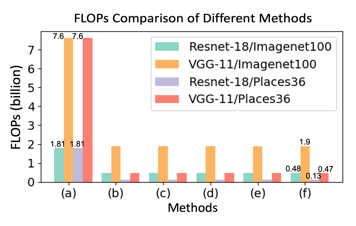
Figure 4. Computation comparison of different methods. For object recognition on Imagenet100, ThumbNet uses $1/4$ FLOPs compared to ‘Original’. For scene recognition on Places36, ThumbNet uses only $1/16$ FLOPs compared to ‘Original’.

Table 4. Accuracy and efficiency comparison with state-of-the-art. B: billion; M: million; MB: MegaBytes. Regarding efficiency, ThumbNet has an obvious advantage over LWAE in terms of all metrics and for all tasks, i.e., ThumbNet requires fewer FLOPs, fewer network parameters, less memory feature maps, and less storage for images. Regarding classification accuracy, ThumbNet has lower top-1 and top-5 errors in the first two tasks. For the third task, ThumbNet has an obviously lower top-5 error and roughly the same top-1 error as LWAE. For the fourth task, LWAE is slightly better than ThumbNet at the cost of higher computational complexity and memory usage.

Tasks	Methods	Error rates		FLOPs		Parameters		Feature Memory		Image Storage
		Top-1	Top-5	# (B)	$\downarrow$ rate	# (M)	$\downarrow$ rate	Size (MB)	$\downarrow$ rate	Size (MB)	$\downarrow$ rate
Imagenet100	VGG-orig	13.64%	4.36%	243.37	1$\times$	129.18	1$\times$	2118.36	1$\times$	4.82	1$\times$
/VGG-11	LWAE (Chen et al., 2018)	17.98%	6.42%	65.61	3.71$\times$	67.78	1.91$\times$	668.94	3.17$\times$	2.41	2$\times$
	ThumbNet	15.72%	4.96%	61.04	3.99$\times$	45.29	2.85$\times$	530.98	3.99$\times$	1.20	4$\times$
Imagenet100	Resnet-orig	17.54%	4.98%	58.04	1$\times$	11.22	1$\times$	658.40	1$\times$	4.82	1$\times$
/Resnet-18	LWAE (Chen et al., 2018)	21.06%	6.90%	17.37	3.34$\times$	11.94	0.94$\times$	212.23	3.10$\times$	2.41	2$\times$
	ThumbNet	17.32%	4.98%	15.52	3.74$\times$	11.22	1$\times$	166.88	3.95$\times$	1.20	4$\times$
Places36	VGG-orig	19.75%	3.61%	243.36	1$\times$	128.91	1$\times$	2118.33	1$\times$	4.82	1$\times$
/VGG-11	LWAE (Chen et al., 2018)	21.53%	4.58%	16.58	14.67$\times$	56.50	2.28$\times$	168.95	12.54$\times$	0.60	8$\times$
	ThumbNet	21.58%	3.72%	15.09	16.13$\times$	28.25	4.56$\times$	133.17	15.91$\times$	0.30	16$\times$
Places36	Resnet-orig	21.11%	3.28%	58.03	1$\times$	11.19	1$\times$	658.38	1$\times$	4.82	1$\times$
/Resnet-18	LWAE (Chen et al., 2018)	22.39%	3.06%	4.48	12.96$\times$	11.91	0.94$\times$	54.51	12.08$\times$	0.60	8$\times$
	ThumbNet	22.78%	3.69%	4.13	14.05$\times$	11.19	1$\times$	42.88	15.35$\times$	0.30	16$\times$

4.2. Comparison to State-of-the-Art Methods

4.2.1. Comparison with LWAE

We compare our ThumbNet to LWAE (Chen et al., 2018) in terms of classification accuracy and resource requirements. Considering that the trained models of LWAE provided by the authors use different backbone networks on different datasets from ours, we re-implement LWAE in Tensorflow (Abadi et al., 2016) (the same as our ThumbNet) with the same backbone networks on the same datasets as ours for fair comparison. We follow the instructions in the paper for setting the hyper-parameters and training LWAE. To evaluate both methods, we test their inference accuracy in terms of top-1 and top-5 error rates, and their inference efficiency in terms of number of FLOPs, number of network parameters, memory consumption of feature maps, and storage requirements for input images.

Table 4 demonstrates the results of testing a batch of $224\times 224$ color images using the two methods as well as the benchmark networks for the four tasks: object recognition on Imagenet100 with VGG-11 and Resnet-18, scene recognition on Places36 with VGG-11 and Resnet-18. For the object recognition tasks, the images are downscaled by 4 in LWAE and ThumbNet; and for the scene recognition tasks, the images are downscaled by 16 in LWAE and ThumbNet. The batch size in these experiments is set to 32.

Seen from Table 4, ThumbNet has an obvious advantage over LWAE in terms of efficiency owing to its one single input image and one single network for inference. ThumbNet only computes one network, whereas LWAE has to compute an extra branch for fusing the high-frequency image. Therefore, when downscaling an image by the same ratio, ThumbNet uses fewer FLOPs, has fewer network parameters, requires less memory for the intermediate feature maps, and stores only one small image (as compared to two images for LWAE). Regarding classification accuracy, ThumbNet has lower top-1 and top-5 errors in the first two tasks. For the third task, ThumbNet has an obviously lower top-5 error and roughly the same top-1 error as LWAE. For the fourth task, LWAE is slightly better than ThumbNet at the cost of higher computational complexity and memory usage.

4.2.2. Comparison with representative network acceleration / compression methods

Table. 5 compares ThumbNet to representative network acceleration/compression methods in recent literature on ImagenetFull/Resnet-50. The results of the comparative methods and their respective baselines are directly taken from the published papers. We can see that the methods SSS (Huang and Wang, 2018), SFP (He et al., 2018) and CP (He et al., 2017) can only speed up by up to 2 times, which is much lower than ThumbNet. The methods ThiNet (Luo et al., 2017), DCP (Zhuang et al., 2018) and Slimmable (Yu et al., 2019) have similar speedup ratios (still lower than) to ThumbNet, but they have obviously higher increase in error rates. Compared to these methods, ThumbNet has obviously lower increase in error rates with even higher acceleration ratios. Moreover, since ThumbNet is orthogonal to conventional acceleration/compression methods, it can be used in conjunction with them for further speedup.

Table 5. ThumbNet compared with representative network compression methods on Imagenet

	Top-1 error		Top-5 error		FLOPs
Methods	Err. %	$\uparrow$	Err. %	$\uparrow$	# B	$\downarrow$
$\textrm{Res50}_{\textrm{SSS}}$	23.88	0/0%	7.14	0/0%	4.09	$1\times$
SSS (Huang and Wang, 2018)	28.18	4.3/18%	9.21	2.07/29%	2.32	$1.76\times$
$\textrm{Res50}_{\textrm{SFP}}$	23.85	0/0%	7.13	0/0%	–	$1\times$
SFP (He et al., 2018)	25.39	1.54/6%	7.94	0.81/11%	–	$1.72\times$
$\textrm{Res50}_{\textrm{CP}}$	–	–	7.8	0/0%	–	$1\times$
CP (He et al., 2017)	–	–	9.2	1.4/18%	–	$2\times$
$\textrm{Resnet50}_{\textrm{Thi}}$	27.12	0/0%	8.86	0/0%	7.72	$1\times$
ThiNet (Luo et al., 2017)	31.58	4.46/16%	11.70	2.84/32%	2.20	$3.51\times$
$\textrm{Resnet50}_{\textrm{DCP}}$	23.99	0/0%	7.07	0/0%	–	$1\times$
DCP (Zhuang et al., 2018)	27.25	3.26/14%	8.87	1.8/25%	–	$3.33\times$
$\textrm{Resnet50}_{\textrm{Slim}}$	23.9	0/0%	–	–	4.1	$1\times$
Slimmable (Yu et al., 2019)	27.9	4.00/17%	–	–	1.1	$3.73\times$
$\textrm{Resnet50}_{\textrm{Thumb}}$	23.59	0/0%	6.90	0/0%	3.86	$1\times$
ThumbNet	26.02	2.43/10%	8.25	1.35/19%	1.02	$\textbf{3.78}\times$

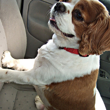
Original

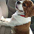
Bicubic

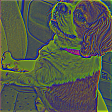
Super. downscaler

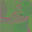
Super. + distillation

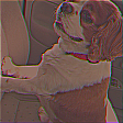
ThumbNet

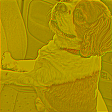
W/o MM

Figure 5. Visual comparison of the thumbnail images generated by different downscalers. ‘Original’ is of size $224\times 224$; the others are $112\times 112$. ‘W/o MM’ means ThumbNet without the MM loss.

4.3. Evaluation of the Supervised Downscaler

4.3.1. Visual Comparison of Downscaled Images

In Fig. 5, we show examples of the generated thumbnail images by our ThumbNet downscalers compared to other different methods for the task of object recognition on Imagenet100 with Resnet-18. We can see that the images of ‘Supervised downscaler’, ‘Supervised + distillation’, ThumbNet, and ‘W/o MM’ (ThumbNet without the MM loss) have noticeable edges compared to the ‘Bicubic’ one. This is because these downscalers are trained in a supervised way with the classification loss being considered. The edge information in the downscaled images is helpful for making discriminative decisions. Also, note that the thumbnail image of ThumbNet is natural in color owing to the MM loss, whereas the image of ‘W/o MM’ is obviously yellowish because the color channels are more easily messed up when the MM loss is not utilized. The top-1 error rates of ThumbNet and ‘W/o MM’ are 17.32% and 17.90%, respectively, and their top-5 error rates are 4.98% and 5.26%, respectively. This shows that adding the MM loss does not deteriorate the network accuracy but produces more pleasant small images, which contain generic information that also benefits other tasks.

4.3.2. Does the Supervised Downscaler Generalize?

In order to verify that the ThumbNet downscaler is also useful apart from being used in the specific inference network $\mathrm{T}$, we also consider three different scenarios for applying our learned downscaler. Suppose that the downscaler is trained on the dataset $A$ with the backbone network $F$. We have a new dataset $A_{new}$ and a different network $F_{new}$. The three scenarios for applying the well-trained downscaler are as follows: (1) downscaling $A$ to generate small images to train $F_{new}$; (2) downscaling $A_{new}$ to generate small images to train $F$; and (3) downscaling $A_{new}$ to generate small images to train $F_{new}$.

Table 6 reports the results of these scenarios using the downscaler learned from the object recognition task with Resnet-18, which downscales an image by 4. In this case, the dataset $A$ is Imagenet100; the network $F$ is Resnet-18. We use Imagenet900 and Caltech256 (Griffin et al., 2007) as the new dataset $A_{new}$, and VGG-11 as the new network $F_{new}$. The first two columns correspond to Scenario (1); the third and fourth columns correspond to Scenario (2); the last two columns correspond to Scenario (3), where we use the downscaler to generate thumbnail images for the new dataset Caltech256, and use these thumbnail images to train a different network VGG-11.

Table 6. Performance of the ThumbNet downscaler on different networks and datasets.

Networks/	VGG-11/		Resnet-18/		VGG-11/
Datasets	Imagenet100		Imagenet900		Caltech256
	Top-1	Top-5	Top-1	Top-5	Top-1	Top-5
Original	13.64	4.36	28.80	10.17	30.68	18.56
Bicubic	18.20	6.60	35.52	14.56	32.80	19.63
ThumbNet	16.74	6.42	33.54	13.22	32.04	18.56

The first row shows the performance of the respective networks trained on the original-size images, while the second row shows their performance when trained on the small images downscaled with bicubic interpolation. The third row shows the performance of the networks trained on the small images downscaled by our ThumbNet downscaler. We can see that the third row obviously outperforms the second row in all scenarios, indicating that our supervised downscaler tends to generalize to other datasets and other network architectures. In fact, it is very promising to see that in Scenario (3) when both the dataset and the network are new to the downscaler, it can still bring about significant gains compared to the bicubic naive downscaler, leading to the same top-5 error rate as the original network.

5. Conclusions

In this paper, we propose a unified framework ThumbNet to tackle the problem of accelerating run-time deep convolutional network from a novel perspective: downscaling the input image. Based on the fact that reducing the input image size lowers the computation and memory costs of a CNN, we seek to obtain a network that can retain original accuracy when applied on one thumbnail image. Experimental results show that, with our ThumbNet, we are able to learn a network that dramatically reduces resource requirements without compromising classification accuracy. Moreover, we have a supervised downscaler as a side product, which can be utilized for generic classification purposes, generalizing to datasets and network architectures that it was not exposed to in training. This work can be used in conjunction with other network acceleration/compression methods for further speed up without incurring additional overheads.

Supplementary Material

1. Details of the datasets Imagenet100 and Places36

1.1. Imagenet100

The 100 categories in Imagenet100 for the object recognition task in Section 4.1.2 are listed as follows

ll n02808440 &  bathtub, bathing tub, bath, tub
n02100877  Irish setter, red setter
n02096585  Boston bull, Boston terrier
n03447721  gong, tam-tam
n03804744  nail
n03930313  picket fence, paling
n03908714  pencil sharpener
n02097298  Scotch terrier, Scottish terrier, Scottie
n04179913  sewing machine
n02169497  leaf beetle, chrysomelid
n04141327  scabbard
n07768694  pomegranate
n03938244  pillow
n04133789  sandal
n04008634  projectile, missile
n01632777  axolotl, mud puppy, Ambystoma mexicanum
n02096177  cairn, cairn terrier
n03000134  chainlink fence
n07860988  dough
n03417042  garbage truck, dustcart
n04550184  wardrobe, closet, press
n04542943  waffle iron
n02487347  macaque
n02007558  flamingo
n04443257  tobacco shop, tobacconist shop, tobacconist
n03902125  pay-phone, pay-station
n04418357  theater curtain, theatre curtain
n02128925  jaguar, panther, Panthera onca, Felis onca
n02101388  Brittany spaniel
n02860847  bobsled, bobsleigh, bob
n13040303  stinkhorn, carrion fungus
n04355338  sundial
n01774384  black widow, Latrodectus mactans
n03657121  lens cap, lens cover
n02708093  analog clock
n04111531  rotisserie
n01829413  hornbill
n04204347  shopping cart
n03792782  mountain bike, all-terrain bike, off-roader
n02268443  dragonfly, darning needle, devil’s darning needle, sewing needle,
 snake feeder, snake doctor, mosquito hawk, skeeter hawk
n03933933  pier
n02879718  bow
n03770439  miniskirt, mini
n03125729  cradle
n03127747  crash helmet
n01728920  ringneck snake, ring-necked snake, ring snake
n03769881  minibus
n04404412  television, television system
n01530575  brambling, Fringilla montifringilla
n04033995  quilt, comforter, comfort, puff
n02102318  cocker spaniel, English cocker spaniel, cocker
n03658185  letter opener, paper knife, paperknife
n01677366  common iguana, iguana, Iguana iguana
n01930112  nematode, nematode worm, roundworm
n01496331  electric ray, crampfish, numbfish, torpedo
n02219486  ant, emmet, pismire
n02437312  Arabian camel, dromedary, Camelus dromedarius
n04258138  solar dish, solar collector, solar furnace
n04596742  wok
n02859443  boathouse
n02356798  fox squirrel, eastern fox squirrel, Sciurus niger
n02777292  balance beam, beam
n12998815  agaric
n02951358  canoe
n03782006  monitor
n03676483  lipstick, lip rouge
n03532672  hook, claw
n02749479  assault rifle, assault gun
n04325704  stole
n04026417  purse
n09256479  coral reef
n07742313  Granny Smith
n01687978  agama
n02835271  bicycle-built-for-two, tandem bicycle, tandem
n01667778  terrapin
n03187595  dial telephone, dial phone
n02113023  Pembroke, Pembroke Welsh corgi
n01739381  vine snake
n02120079  Arctic fox, white fox, Alopex lagopus
n02056570  king penguin, Aptenodytes patagonica
n04435653  tile roof
n01749939  green mamba
n03207941  dishwasher, dish washer, dishwashing machine
n07831146  carbonara
n04604644  worm fence, snake fence, snake-rail fence, Virginia fence
n02927161  butcher shop, meat market
n01630670  common newt, Triturus vulgaris
n03598930  jigsaw puzzle
n03691459  loudspeaker, speaker, speaker unit, loudspeaker system, speaker system
n02114855  coyote, prairie wolf, brush wolf, Canis latrans
n02791270  barbershop
n01484850  great white shark, white shark, man-eater, man-eating shark, Carcharodon carcharias
n04146614  school bus
n04356056  sunglasses, dark glasses, shades
n02086646  Blenheim spaniel
n02110627  affenpinscher, monkey pinscher, monkey dog
n03854065  organ, pipe organ
n03697007  lumbermill, sawmill
n02454379  armadillo
n03314780  face powder

1.2. Places36

The 36 categories in Places36 for the scene recognition tasks in Section 4.1.3 are listed as follows

ll 307 &  /s/skyscraper
29  /a/auto_showroom
195  /j/jacuzzi/indoor
13  /a/archaelogical_excavation
108  /c/courthouse
16  /a/arena/performance
1  /a/airplane_cabin
38  /b/banquet_hall
175  /h/highway
268  /p/playground
129  /e/elevator/door
142  /f/field_road
123  /d/doorway/outdoor
11  /a/arcade
338  /t/tree_farm
151  /f/forest_path
47  /b/bazaar/outdoor
140  /f/field/cultivated
181  /h/hotel/outdoor
107  /c/cottage
155  /g/galley
178  /h/hospital
51  /b/bedchamber
4  /a/alley
141  /f/field/wild
262  /p/pharmacy
297  /s/science_museum
79  /c/canal/urban
254  /p/park
293  /r/runway
100  /c/computer_room
99  /c/coffee_shop
210  /l/lecture_room
362  /y/yard
45  /b/bathroom
211  /l/legislative_chamber

References

- (1)
- Abadi et al. (2016) Martín Abadi, Paul Barham, Jianmin Chen, Zhifeng Chen, Andy Davis, Jeffrey Dean, Matthieu Devin, Sanjay Ghemawat, Geoffrey Irving, Michael Isard, et al. 2016. TensorFlow: A System for Large-Scale Machine Learning.. In OSDI, Vol. 16. 265–283.
- Bourlard and Kamp (1988) Hervé Bourlard and Yves Kamp. 1988. Auto-association by multilayer perceptrons and singular value decomposition. Biological cybernetics 59, 4-5 (1988), 291–294.
- Canziani et al. (2016) Alfredo Canziani, Adam Paszke, and Eugenio Culurciello. 2016. An analysis of deep neural network models for practical applications. arXiv preprint arXiv:1605.07678 (2016).
- Chen et al. (2017) Guobin Chen, Wongun Choi, Xiang Yu, Tony Han, and Manmohan Chandraker. 2017. Learning Efficient Object Detection Models with Knowledge Distillation. In Advances in Neural Information Processing Systems. 742–751.
- Chen et al. (2018) Tianshui Chen, Liang Lin, Wangmeng Zuo, Xiaonan Luo, and Lei Zhang. 2018. Learning a Wavelet-like Auto-Encoder to Accelerate Deep Neural Networks. In AAAI.
- Courbariaux et al. (2016) Matthieu Courbariaux, Itay Hubara, Daniel Soudry, Ran El-Yaniv, and Yoshua Bengio. 2016. Binarized neural networks: Training deep neural networks with weights and activations constrained to+ 1 or-1. arXiv preprint arXiv:1602.02830 (2016).
- Deng et al. (2009) J. Deng, W. Dong, R. Socher, L.-J. Li, K. Li, and L. Fei-Fei. 2009. ImageNet: A Large-Scale Hierarchical Image Database. In CVPR09.
- Denton et al. (2014) Emily L Denton, Wojciech Zaremba, Joan Bruna, Yann LeCun, and Rob Fergus. 2014. Exploiting linear structure within convolutional networks for efficient evaluation. In Advances in neural information processing systems. 1269–1277.
- Erhan et al. (2010) Dumitru Erhan, Yoshua Bengio, Aaron Courville, Pierre-Antoine Manzagol, Pascal Vincent, and Samy Bengio. 2010. Why does unsupervised pre-training help deep learning? Journal of Machine Learning Research 11, Feb (2010), 625–660.
- Griffin et al. (2007) Gregory Griffin, Alex Holub, and Pietro Perona. 2007. Caltech-256 object category dataset. (2007).
- Han et al. (2016) Song Han, Huizi Mao, and William J. Dally. 2016. Deep Compression: Compressing Deep Neural Network with Pruning, Trained Quantization and Huffman Coding. International Conference on Learning Representations ICLR abs/1510.00149 (2016).
- He and Sun (2015) Kaiming He and Jian Sun. 2015. Convolutional neural networks at constrained time cost. In Computer Vision and Pattern Recognition (CVPR), 2015 IEEE Conference on. IEEE, 5353–5360.
- He et al. (2016) Kaiming He, Xiangyu Zhang, Shaoqing Ren, and Jian Sun. 2016. Deep residual learning for image recognition. In Proceedings of the IEEE conference on computer vision and pattern recognition. 770–778.
- He et al. (2018) Yang He, Guoliang Kang, Xuanyi Dong, Yanwei Fu, and Yi Yang. 2018. Soft Filter Pruning for Accelerating Deep Convolutional Neural Networks. ArXiv abs/1808.06866 (2018).
- He et al. (2017) Yihui He, Xiangyu Zhang, and Jian Sun. 2017. Channel Pruning for Accelerating Very Deep Neural Networks. 2017 IEEE International Conference on Computer Vision (ICCV) (2017), 1398–1406.
- Hinton et al. (2015) Geoffrey Hinton, Oriol Vinyals, and Jeff Dean. 2015. Distilling the knowledge in a neural network. arXiv preprint arXiv:1503.02531 (2015).
- Hinton and Salakhutdinov (2006) Geoffrey E Hinton and Ruslan R Salakhutdinov. 2006. Reducing the dimensionality of data with neural networks. Science 313, 5786 (2006), 504–507.
- Huang and Wang (2018) Zehao Huang and Naiyan Wang. 2018. Data-Driven Sparse Structure Selection for Deep Neural Networks. In ECCV.
- Ioffe and Szegedy (2015) Sergey Ioffe and Christian Szegedy. 2015. Batch normalization: Accelerating deep network training by reducing internal covariate shift. In International conference on machine learning. 448–456.
- Jaderberg et al. (2014) Max Jaderberg, Andrea Vedaldi, and Andrew Zisserman. 2014. Speeding up convolutional neural networks with low rank expansions. arXiv preprint arXiv:1405.3866 (2014).
- Lavin and Gray (2016) Andrew Lavin and Scott Gray. 2016. Fast algorithms for convolutional neural networks. In Proceedings of the IEEE Conference on Computer Vision and Pattern Recognition. 4013–4021.
- Lebedev et al. (2014) Vadim Lebedev, Yaroslav Ganin, Maksim Rakhuba, Ivan Oseledets, and Victor Lempitsky. 2014. Speeding-up convolutional neural networks using fine-tuned cp-decomposition. arXiv preprint arXiv:1412.6553 (2014).
- LeCun et al. (1990) Yann LeCun, John S Denker, and Sara A Solla. 1990. Optimal brain damage. In Advances in Neural Information Processing Systems. 598–605.
- Lehmann et al. (1999) Thomas Martin Lehmann, Claudia Gonner, and Klaus Spitzer. 1999. Survey: Interpolation methods in medical image processing. IEEE Transactions on Medical Imaging 18, 11 (1999), 1049–1075.
- Li et al. (2016) Hao Li, Asim Kadav, Igor Durdanovic, Hanan Samet, and Hans Peter Graf. 2016. Pruning filters for efficient convnets. arXiv preprint arXiv:1608.08710 (2016).
- Li et al. (2015) Yujia Li, Kevin Swersky, and Rich Zemel. 2015. Generative moment matching networks. In International Conference on Machine Learning. 1718–1727.
- Li et al. (2017) Yanghao Li, Naiyan Wang, Jiaying Liu, and Xiaodi Hou. 2017. Demystifying neural style transfer. arXiv preprint arXiv:1701.01036 (2017).
- Luo et al. (2017) Jian-Hao Luo, Jianxin Wu, and Weiyao Lin. 2017. ThiNet: A Filter Level Pruning Method for Deep Neural Network Compression. 2017 IEEE International Conference on Computer Vision (ICCV) (2017), 5068–5076.
- Masci et al. (2011) Jonathan Masci, Ueli Meier, Dan Cireşan, and Jürgen Schmidhuber. 2011. Stacked convolutional auto-encoders for hierarchical feature extraction. In International Conference on Artificial Neural Networks. Springer, 52–59.
- Mathieu et al. (2013) Michael Mathieu, Mikael Henaff, and Yann LeCun. 2013. Fast training of convolutional networks through ffts. arXiv preprint arXiv:1312.5851 (2013).
- Nair and Hinton (2010) Vinod Nair and Geoffrey E Hinton. 2010. Rectified linear units improve restricted boltzmann machines. In Proceedings of the 27th International Conference on Machine Learning (ICML-10). 807–814.
- Papernot et al. (2016) Nicolas Papernot, Patrick McDaniel, Xi Wu, Somesh Jha, and Ananthram Swami. 2016. Distillation as a defense to adversarial perturbations against deep neural networks. In Security and Privacy (SP), 2016 IEEE Symposium on. IEEE, 582–597.
- Rastegari et al. (2016) Mohammad Rastegari, Vicente Ordonez, Joseph Redmon, and Ali Farhadi. 2016. Xnor-net: Imagenet classification using binary convolutional neural networks. In European Conference on Computer Vision. Springer, 525–542.
- Romero et al. (2014) Adriana Romero, Nicolas Ballas, Samira Ebrahimi Kahou, Antoine Chassang, Carlo Gatta, and Yoshua Bengio. 2014. Fitnets: Hints for thin deep nets. arXiv preprint arXiv:1412.6550 (2014).
- Simonyan and Zisserman (2015) Karen Simonyan and Andrew Zisserman. 2015. Very Deep Convolutional Networks for Large-Scale Image Recognition. International Conference on Learning Representations ICLR (2015).
- Turchenko et al. (2017) Volodymyr Turchenko, Eric Chalmers, and Artur Luczak. 2017. A Deep Convolutional Auto-Encoder with Pooling-Unpooling Layers in Caffe. arXiv preprint arXiv:1701.04949 (2017).
- Wu et al. (2016) Jiaxiang Wu, Cong Leng, Yuhang Wang, Qinghao Hu, and Jian Cheng. 2016. Quantized convolutional neural networks for mobile devices. In Proceedings of the IEEE Conference on Computer Vision and Pattern Recognition. 4820–4828.
- Xie et al. (2017) Saining Xie, Ross Girshick, Piotr Dollár, Zhuowen Tu, and Kaiming He. 2017. Aggregated residual transformations for deep neural networks. In Proceedings of the IEEE conference on Computer Vision and Pattern Recognition. 1492–1500.
- Xu et al. (2020) Mengmeng Xu, Chen Zhao, David S Rojas, Ali Thabet, and Bernard Ghanem. 2020. G-TAD: Sub-Graph Localization for Temporal Action tion. In Proceedings of the IEEE/CVF Conference on Computer Vision and Pattern Recognition. 10156–10165.
- Yu et al. (2019) Jiahui Yu, Linjie Yang, Ning Xu, Jianchao Yang, and Thomas Huang. 2019. Slimmable Neural Networks. In International Conference on Learning Representations. https://openreview.net/forum?id=H1gMCsAqY7
- Zeiler et al. (2010) Matthew D Zeiler, Dilip Krishnan, Graham W Taylor, and Rob Fergus. 2010. Deconvolutional networks. In Computer Vision and Pattern Recognition (CVPR), 2010 IEEE Conference on. IEEE, 2528–2535.
- Zhang et al. (2014) Jian Zhang, Chen Zhao, Debin Zhao, and Wen Le Gao. 2014. Image compressive sensing recovery using adaptively learned sparsifying basis via L0 minimization. Signal Process. 103 (2014), 114–126.
- Zhang et al. (2012) Jian Zhang, Debin Zhao, Chen Zhao, Ruiqin Xiong, Siwei Ma, and Wen Gao. 2012. Image Compressive Sensing Recovery via Collaborative Sparsity. IEEE Journal on Emerging and Selected Topics in Circuits and Systems 2 (2012), 380–391.
- Zhang et al. (2016) Xiangyu Zhang, Jianhua Zou, Kaiming He, and Jian Sun. 2016. Accelerating very deep convolutional networks for classification and detection. IEEE Transactions on Pattern Analysis and Machine Intelligence 38, 10 (2016), 1943–1955.
- Zhao et al. (2014) Chen Zhao, Siwei Ma, and Wen Gao. 2014. Image compressive-sensing recovery using structured laplacian sparsity in DCT domain and multi-hypothesis prediction. 2014 IEEE International Conference on Multimedia and Expo (ICME) (2014), 1–6.
- Zhao et al. (2017a) Chen Zhao, Siwei Ma, Jian Zhang, Ruiqin Xiong, and Wen Gao. 2017a. Video Compressive Sensing Reconstruction via Reweighted Residual Sparsity. IEEE Transactions on Circuits and Systems for Video Technology 27 (2017), 1182–1195.
- Zhao et al. (2017b) Chen Zhao, Ronggang Wang, and Wen Gao. 2017b. Better and faster, when ADMM meets CNN: compressive-sensed image reconstruction. In Pacific Rim Conference on Multimedia. Springer, 370–379.
- Zhao et al. (2013) Chen Zhao, Jian Zhang, Siwei Ma, and Wen Gao. 2013. Wavelet inpainting driven image compression via collaborative sparsity at low bit rates. In 2013 IEEE International Conference on Image Processing. IEEE, 1685–1689.
- Zhao et al. (2016) Chen Zhao, Jian Zhang, Siwei Ma, and Wen Gao. 2016. Nonconvex Lp Nuclear Norm based ADMM Framework for Compressed Sensing. 2016 Data Compression Conference (DCC) (2016), 161–170.
- Zhao et al. (2018a) Chen Zhao, Jian Zhang, Ronggang Wang, and Wen Gao. 2018a. BoostNet: A Structured Deep Recursive Network to Boost Image Deblocking. In 2018 IEEE Visual Communications and Image Processing (VCIP). IEEE, 1–4.
- Zhao et al. (2018b) Chen Zhao, Jian Zhang, Ronggang Wang, and Wen Gao. 2018b. CREAM: CNN-REgularized ADMM framework for compressive-sensed image reconstruction. IEEE Access 6 (2018), 76838–76853.
- Zhou et al. (2017) Bolei Zhou, Agata Lapedriza, Aditya Khosla, Aude Oliva, and Antonio Torralba. 2017. Places: A 10 million Image Database for Scene Recognition. IEEE Transactions on Pattern Analysis and Machine Intelligence (2017).
- Zhuang et al. (2018) Zhuangwei Zhuang, Mingkui Tan, Bohan Zhuang, Jing Liu, Yong Guo, Qingyao Wu, Junzhou Huang, and Jin-Hui Zhu. 2018. Discrimination-aware Channel Pruning for Deep Neural Networks. In NeurIPS.