Magnetohydrodynamics in a Cylindrical Shearing Box

Abstract

We develop a framework for magnetohydrodynamical (MHD) simulations in a local cylindrical shearing box by extending the formulation of the Cartesian shearing box. We construct shearing-periodic conditions at the radial boundaries of a simulation box from the conservation relations of the basic MHD equations, taking into account the explicit radial dependence of physical quantities. We demonstrate quasi-steady mass accretion, which cannot be handled by the standard Cartesian shearing box model, with an ideal MHD simulation in a vertically unstratified cylindrical shearing box up to 200 rotations. In this demonstrative run we set up (i) net vertical magnetic flux, (ii) a locally isothermal equation of state, and (iii) a sub-Keplerian equilibrium rotation, whereas the sound velocity and the initial Alfvén velocity have the same radial dependence as that of the Keplerian velocity. Inward mass accretion is induced to balance with the outward angular momentum flux of the MHD turbulence triggered by the magnetorotational instability in a self-consistent manner. We discuss detailed physical properties of the saturated magnetic field, in comparison to the results of a Cartesian shearing box simulation.

1 Introduction

Accretion disks are ubiquitously formed around gravitational objects such as black holes, neutron stars, white dwarfs, and pre-main-sequence stars. Material in the inner part of a disk accretes onto a central object. In order to induce the mass accretion, the angular momentum has to be transported outward (Lynden-Bell & Pringle, 1974). The molecular viscosity is insufficient to account for the required transport rate of angular momentum, because the Reynolds number of astrophysical objects is huge. Therefore, macroscopic processes should operate in order to trigger mass accretion.

(Magneto)hydrodynamical ((M)HD hereafter) turbulence has been highlighted, because it works as an effective viscosity to transport angular momentum (e.g., Balbus & Hawley, 1991, 1998; Blackman & Nauman, 2015). Magnetized disk winds, which remove angular momentum from a disk in the vertical direction, have also been widely discussed (Blandford & Payne, 1982; Pelletier & Pudritz, 1992). Since these processes involve nonlinear phenomena, MHD simulations have been performed to investigate the transfer of mass and angular momentum (e.g., Hawley, 2000; Machida et al., 2000; Penna et al., 2010; Li et al., 2011; Parkin & Bicknell, 2013; Tomida et al., 2015; Takasao et al., 2018; Suriano et al., 2019).

Local shearing box simulations have been widely used to examine fine-scale MHD turbulence excited by the magnetorotational instability (MRI; Velikhov, 1959; Chandrasekhar, 1961; Balbus & Hawley, 1991) by zooming in on a local patch of an accretion disk (Hawley et al., 1995; Matsumoto & Tajima, 1995). By taking into account vertical stratification (Brandenburg et al., 1995; Stone et al., 1996) the local treatment is applied to studying the saturation of amplified magnetic fields (e.g., Sano et al., 2004; Fromang & Papaloizou, 2007; Davis et al., 2010), driving vertical outflows and disk winds (Suzuki & Inutsuka, 2009; Bai & Stone, 2013a; Fromang et al., 2013; Lesur et al., 2013) and heating coronae (Miller & Stone, 2000; Io & Suzuki, 2014). It has been also extended further by including various physical processes of radiative effects (Turner et al., 2003; Hirose et al., 2006; Jiang et al., 2013), dynamics of dust grains (Johansen et al., 2006; Taki et al., 2016), non-ideal MHD effects (Sano & Stone, 2002; Sano et al., 2004; Turner et al., 2007; Okuzumi & Hirose, 2012; Bai & Stone, 2013b; Simon et al., 2015), and acceleration of high-energy particles (Hoshino, 2015; Kimura et al., 2016) in various types of accretion disks. The local approach does not only apply to accretion disks but also to proto-neutron stars that are formed through core-collapse supernovae (Masada et al., 2012; Rembiasz et al., 2016).

Thus, this local approach has achieved great successes in various applications. However, this does not mean that the local shearing box is a perfect approach. In the shearing box approximation, the focus is small-scale phenomena, which the curvature of a disk can be neglected, and local Cartesian coordinates are adopted. A simulation box rotates with the equilibrium rotation velocity at the origin of the box, and the radial direction is usually taken as the $x$ axis. The Cartesian shearing coordinates have a strict symmetry across the $x=0$ plane. While a central object is usually put in the $-x$ region, it would be correct to regard that central object as actually located in the $+x$ region of the same simulation, because there is no preferred direction with respect to the $x$ axis.

Therefore, mass accretion cannot be directly captured in the Cartesian shearing box; the integrated net mass flux across both ends of the $x$ boundaries should be strictly zero in a well constructed Cartesian shearing box simulation. The mass accretion rate cannot be measured directly from these simulations but instead it is estimated from the $xy$ (radial-azimuthal) component of a stress tensor based on the balance of angular momentum flux (see Sub-subsection 4.2.3).

It is key to take into account the curvature of the disk to break the $\pm x$ symmetry for a more realistic treatment. Brandenburg et al. (1996) restored the terms arising from the curvature in their Cartesian box simulation and reported that it actually realized net mass accretion. Klahr & Bodenheimer (2003) introduced a framework of shearing disks for their radiation HD simulation in spherical coordinates, in which shearing periodic conditions are applied with explicit radial dependences of physical quantities at the radial boundaries of a simulation box. Based on this framework, Obergaulinger et al. (2009) performed semi-global MHD simulations in cylindrical coordinates for the MRI in core-collapse supernovae. While their works turned out to be great steps forward, the numerical implementation is not still well matured; at the moment “damping zones” need to be prepared at the radial boundaries to suppress troublesome oscillatory behavior of a simulation box.

We extend the basic strategy of the shearing disk by utilizing the basis conservation relations of mass, momentum, energy, and magnetic field in an explicit manner. We directly apply them to shearing periodic conditions at the radial boundaries of a local cylindrical simulation box. Without prescribing a damping treatment at the radial boundaries, our simulation naturally realizes the mass accretion that is balanced with the outwardly transported angular momentum by MHD turbulence. We successfully incorporate the global effects, while keeping the merits of the local approach that can capture fine-scale turbulence in simulations that remain stable over long timescales.

We present the formulation of cylindrical shearing box simulations in Section 2. The numerical implementation is described in Section 3 and Appendix C. We demonstrate one case of the simulation up to 200 rotation periods, in comparison to results of a Cartesian shearing box, in Section 4. We discuss several future directions of our framework in Section 5 and summarize the paper in Section 6.

2 Cylindrical Shearing Box

2.1 Basic Equations

We perform an MHD simulation in cylindrical coordinates, $(R,\phi,z)$, with the rotation axis along the $z$ direction. The simulation box covers a region of $(R_{-}\leq R\leq R_{+},\phi_{-}\leq\phi\leq\phi_{+},z_{-}\leq z\leq z_{+})$ and rotates with the equilibrium rotation frequency, $\mbox{\boldmath${\Omega}$}_{\rm eq,0}=\Omega_{\rm eq,0}\hat{z}$, at $R=R_{0}$ (see eqs.35 & 37), where the “hat” stands for a unit vector. We usually take $R_{-}<R_{0}<R_{+}$ but $R_{0}$ does not necessarily equal $(R_{-}+R_{+})/2$. We restrict our simulation to regions near the midplane and neglect the vertical component of the gravity in this paper. We solve MHD evolutionary equations,

$$\frac{d\rho}{dt}+\rho\mbox{\boldmath${\nabla}$}\cdot\mbox{\boldmath${v}$}=0,$$ (1)

$$\rho\frac{d\mbox{\boldmath${v}$}}{dt}=-\mbox{\boldmath${\nabla}$}\left(p+\frac{B^{2}}{8\pi}\right)+\left(\frac{\mbox{\boldmath${B}$}}{4\pi}\cdot\mbox{\boldmath${\nabla}$}\right)\mbox{\boldmath${B}$}-\rho\frac{GM_{\star}}{R^{2}}\hat{R}$$

$$+\rho\mbox{\boldmath${R}$}\Omega_{\rm eq,0}^{2}-2\rho\mbox{\boldmath${\Omega}$}_{\rm eq,0}\mbox{\boldmath${\times}$}\mbox{\boldmath${v}$}$$ (2)

and

$$\frac{\partial\mbox{\boldmath${B}$}}{\partial t}=\mbox{\boldmath${\nabla\times(v\times B)}$},$$ (3)

under a constraint equation of

$$\mbox{\boldmath${\nabla\cdot B}$}=0,$$ (4)

with an isothermal equation of state,

$$p=\rho c_{\rm s}^{2},$$ (5)

in the frame that rotates with $\Omega_{\rm eq,0}$. Here, $\rho$, $p$, ${v}$, and ${B}$ are density, gas pressure, velocity, and magnetic field, $G$ is the gravitational constant, $M_{\star}$ is the mass of a central star, and $c_{\rm s}$ is isothermal sound speed. $\frac{d}{dt}$ and $\frac{\partial}{\partial t}$ denote Lagrangian and Eulerian time derivatives, respectively. We adopt a locally isothermal approximation: $c_{\rm s}$ depends only on spacial locations and does not evolve with time (see Section 3 for the detail). We describe the numerical implementation of the gravity, the centrifugal force, and the Coriolis force in the radial momentum equation in Appendix A.

The velocity measured in this corotating frame, ${v}$ is related to the velocity measured in the rest frame, ${u}$, via

$$\mbox{\boldmath${v}$}=\mbox{\boldmath${u}$}-R\Omega_{\rm eq,0}\hat{\phi},$$ (6)

and therefore, the azimuthal velocity in the corotating frame is expressed as

$$v_{\phi}=R(\Omega-\Omega_{\rm eq,0}),$$ (7)

where $\mbox{\boldmath${\Omega}$}(R)=\Omega\hat{z}$ is the angular velocity measured from the rest frame.

2.2 Shearing Boundary Condition in Cylindrical Coordinates

A key in our framework of the cylindrical shearing box is how to prescribe the shearing condition at the radial boundaries. We basically extend the shearing condition for Cartesian coordinates (Hawley et al., 1995) to cylindrical coordinates. In order to do so, we calculate the shear between $R_{-}$ and $R_{+}$ by the angular difference, which gives the following shearing periodic boundary condition for a variable, $S$:

$$S(R_{\pm},\phi,z) = S(R_{\mp},\phi-(\Omega_{\rm eq,\pm}-\Omega_{\rm eq,\mp})t,z)$$ (8)

$$= S(R_{\mp},\phi\pm\Delta\Omega_{\rm eq}t,z),$$

where $\Omega_{\rm eq,-}$ ($\Omega_{\rm eq,+}$) is the equilibrium angular speed at the inner (outer) radial boundary, $R_{-}$ ($R_{+}$), and $\Delta\Omega_{\rm eq}=\Omega_{\rm eq,-}-\Omega_{\rm eq,+}$, which is positive for inner fast rotation.

We need to carefully select shearing variables, $S$, from the conservation laws of mass, momentum, energy, and magnetic field. Although the condition of the energy is not necessary in the present paper because we assume the locally isothermal equation of state (eq.5), we present the formalism for the energy conservation for completeness.

Conservative forms of the basic equations are presented in Appendix B.1. Radial differential terms in these equations should be treated with a special care for the shearing periodic boundary condition.

Mass

The first shearing variable is from the continuity equation (eqs. 1 and 56):

$$S_{\rm mass}=\rho v_{R}R,$$ (9)

which conserves the total mass in the simulation box.

Radial Momentum

The conservation of radial momentum can be realized by using radial differential terms in eq.(57) of Appendix A. However, we do not impose the strict conservation on the radial momentum flux in order to handle net mass accretion. We start our simulation from the equilibrium profile described in Subsection 3.4, which indicates that the initial net radial momentum flux is zero. Therefore, if we impose the conservation of the total radial momentum flux in the simulation box, mass accretion cannot be induced, which is not the purpose of the present work.

In order to handle mass accretion, we loosen the conservation condition. In the shearing variable of the radial momentum flux we do not take into account the curvature term, $u_{\phi}^{2}/R$, of eq.(57) in the rest frame, which mostly corresponds to the centrifugal force in the corotating frame. The centrifugal force is a dominant term in the radial force balance, in addition to the gravity and the pressure gradient force. When the azimuthal velocity is decelerated, the inward flow of gas is triggered. We determine the shearing condition of $v_{\phi}$ from the angular momentum flux in order that net accretion is realized, which is described later.

Also, we do not consider the terms concerning ${B}$ in eq.(57) in the shearing variables because the contribution from these terms are not so significant (However, they may affect long-time behavior; see Appendix C for the detail).

We use the radial dynamical pressure as a simple choice:

$$S_{{\rm mom},R}=\rho v_{R}^{2}R,$$ (10)

In this setup, radial gas motion is not excited by the dynamical pressure but mainly by the change of angular momentum and a small contribution from the magnetic pressure.

Angular Momentum

Angular momentum flux directed to the radial direction is expressed as

$${\cal L}_{R\phi} = \left(\rho u_{R}u_{\phi}-\frac{1}{4\pi}B_{R}B_{\phi}\right)R$$ (11)

$$= \rho v_{R}R(R\Omega_{\rm eq})+\left(\rho v_{R}\delta v_{\phi}-\frac{1}{4\pi}B_{R}B_{\phi}\right)R$$

$$\equiv \rho v_{R}R(R\Omega_{\rm eq})+w_{R\phi}R$$

in the rest frame (see eq.58), where

$$\delta v_{\phi}=v_{\phi}-v_{\phi,{\rm eq}}$$ (12)

is the difference of $v_{\phi}$ from the local equilibrium azimuthal velocity, $v_{\phi,{\rm eq}}=R(\Omega_{\rm eq}-\Omega_{\rm eq,0})$, and

$$w_{R\phi}=\rho v_{R}\delta v_{\phi}-\frac{1}{4\pi}B_{R}B_{\phi}$$ (13)

is the $R\phi$ component of MHD stress tensor. $w_{R\phi}$ is often discussed in terms of the $\alpha$ prescription (Shakura & Sunyaev, 1973) as $w_{R\phi}=\alpha\rho c_{\rm s}^{2}$.

The first term on the right-hand side denotes the angular momentum advected by radial mass flow, and the second term corresponds to the angular momentum transported by MHD turbulence. When the mass accretes inward by the outward transport of angular momentum by turbulence as in standard accretion disks (Shakura & Sunyaev, 1973), the first term is negative and the second term is positive.

The difference between ${\cal L}_{R\phi}R$ at $R_{-}$ and ${\cal L}_{R\phi}R$ at $R_{+}$ determines the variation of the total angular momentum in the simulation box (eq.58). If $({\cal L}_{R\phi}R)_{+}=({\cal L}_{R\phi}R)_{-}$ is imposed, the total angular momentum is conserved. In this case the radial force balance is maintained because the centrifugal force, which balances with the gravity and the pressure gradient force, does not change with time. Therefore, if $({\cal L}_{R\phi}R)_{+}=({\cal L}_{R\phi}R)_{-}$ is applied, mass does not accrete, which is not what we want to model.

We allow the change of the total angular momentum in order to generate net mass accretion. However, after the magnetic field is amplified to be in the quasi-saturated state, time-steady mass accretion should be realized. In order to fulfill these conflicting demands, we will have to prescribe a shearing boundary condition that satisfies $({\cal L}_{R\phi})_{+}\approx({\cal L}_{R\phi})_{-}$ after the saturated state is achieved, while we have to loosen the strict conservation constraint, $({\cal L}_{R\phi}R)_{+}=({\cal L}_{R\phi}R)_{-}$.

The first term on the right-hand side, $\rho v_{R}R(R\Omega_{\rm eq})$, has a negative value and is proportional to $(R\Omega_{\rm eq})$ in the steady accretion phase, $\rho v_{R}R(<0)=$ const. (eq.9). On the other hand, the second term, $w_{R\phi}R$, is positive, and if $w_{R\phi}R=-\rho v_{R}R(R\Omega_{\rm eq})$ at $R=R_{\pm}$, the gas in the simulation box does neither gains nor loses angular momentum.

Based on this consideration, we adopt a shearing variable for the angular momentum,

$$S_{\rm mom,\phi}=w_{R\phi}/\Omega_{\rm eq}.$$ (14)

Although this choice allows the gain or loss of the angular momentum, in the steady-state accreting phase of $\rho v_{R}R=$const., it gives $w_{R\phi}R^{2}$ & ${\cal L}_{R\phi}R\propto R^{2}\Omega_{\rm eq}$ (eq.11). We note that $|{\cal L}_{R\phi}R|$ is an increasing function of $R$ because specific angular momentum, $R^{2}\Omega_{\rm eq}$, increases with $R$. (If this is not satisfied, the system is dynamically unstable, since it breaks the Rayleigh’s stability criterion.)

Let us consider a case in which ${\cal L}_{R\phi}R$ is negative. In this case the total angular momentum increases because the angular momentum that flows out of $R_{-}$ is smaller than the incoming angular momentum from $R_{+}$. As a result, the mass accretion is eventually reduced ($v_{R}$ increases), which increases ${\cal L}_{R\phi}R$. On the other hand, if ${\cal L}_{R\phi}R$ is positive, the total angular momentum decreases because the angular momentum that flows out of $R_{+}$ is larger than the incoming angular momentum from $R_{-}$. Hence, mass accretion is eventually increased ($v_{R}$ decreases), and ${\cal L}_{R\phi}R$ declines.

We expect that the choice of eq.(14) leads to ${\cal L}_{R\phi}R\approx 0$ in a self-regulating manner after the different components of ${\cal L}_{R\phi}R$ are canceled out. However, this argument is based on our theoretical consideration, and hence, we have to check whether this self-regulation is actually realized by numerical simulation.

We describe our specific method for how to numerically prescribe the shearing condition of $S_{\rm mom,\phi}$ in Appendix C.2. In short, we assume both the Reynolds and Maxwell stresses have the same scaling on $R$, $\rho v_{R}\delta v_{\phi}\propto\Omega_{\rm eq}$ and $B_{R}B_{\phi}\propto\Omega_{\rm eq}$. The condition for the Reynolds stress gives

$$\delta v_{\phi}\propto R\Omega_{\rm eq}$$ (15)

for the constraint of mass conservation, $\rho v_{R}\propto R^{-1}$ (eq.9).

Vertical Momentum

The shearing condition for vertical velocity is obtained from the radial differential terms of eq.(59). Here, we use the only HD term and neglect the magnetic effect ($\partial_{R}(B_{R}B_{z}R)$), because the latter is generally small in the unstratified setting. We use

$$S_{{\rm mom},z}=\rho v_{R}v_{z}R.$$ (16)

as a shearing variable for the vertical momentum.

Magnetic Field

Similarly to the HD variables, the radial differential terms of the induction equation should be used as shearing variables, which are the $z$ component of induction electric field,

$$S_{B_{\phi}}=cE_{z}=v_{R}B_{\phi}-v_{\phi}B_{R},$$ (17)

in the evolutionary equation of $B_{\phi}$ (eq.61), and the $\phi$ component of induction electric field,

$$S_{B_{z}}=RcE_{\phi}=R(v_{z}B_{R}-v_{R}B_{z}),$$ (18)

in the evolutionary equation of $B_{z}$ (eq.62), where $c$ is the speed of light. Here, we note that the induction equations in the corotating frame can be derived by replacing $u_{\phi}$ with $v_{\phi}$ of eqs.(60) – (62) in the rest frame (see Appendix B.2). Besides these two shearing variables, the constraint equation (4) determines the three components of magnetic field.

Energy

The radial differential term of the total energy equation (64) can be used as a shearing variable for energy. Because the contribution from magnetic field is usually small,

$$S_{\rm eng}=\rho v_{R}R\left[\frac{v^{2}}{2}+(\gamma-1)e\right]$$ (19)

can be a reasonable shearing variable, where $\gamma$ is the ratio of specific heats and we used the relation, $p=(\gamma-1)\rho e$.

However, as we stated above, we assume that the gas is locally isothermal (see Section 3 for the detail) and we do not solve the energy equation. Therefore, we do not use $S_{\rm eng}$ for the radial shearing boundary condition in this paper.

Summary of Shearing Variables

We set up the seven shearing variables, eqs.(9), (10), (14)–(19). The eight primitive variables, $\rho$, ${v}$, ${B}$, and $e$ for the shearing periodic condition are in principle determined by these seven conditions and the constraint of $\mbox{\boldmath${\nabla\cdot B}$}=0$ (eq.4). A specific implementation method needs to be carefully constructed in order that it is compatible with an adopted MHD scheme. We describe our method in Subsection 3.3 and Appendix C.2.

2.3 Periodic Boudary for $\phi$ and $z$ Components

We adopt the periodic boundary condition for a variable, $A$, at the $\phi$ and $z$ boundaries, as usually taken in unstratifed Cartesian shearing box simulations (Hawley et al., 1995, and more),

$$A(R,\phi_{\pm},z)=A(R,\phi_{\mp},z)$$ (20)

and

$$A(R,\phi,z_{\pm})=A(R,\phi,z_{\mp}).$$ (21)

For the $\phi$ and $z$ boundaries, we take primitive variables for $A=\rho,\mbox{\boldmath${v}$},\mbox{\boldmath${B}$}$, and $e$.

2.4 Constraints & Conserved Quantities

We can obtain constraints and conserved quantities from the shearing periodic boundary condition for the $R$ direction (Subsection 2.2) and the simple periodic boundary condition for the $\phi$ and $z$ directions (§2.3). The shearing condition of $S_{\rm mass}$ (eq.9) ensures the conservation of the mass in the simulation box

$$M=[\rho]_{{}_{V}}=\int_{z_{-}}^{z_{+}}\int_{\phi_{-}}^{\phi_{+}}\int_{R_{-}}^{R_{+}}\rho RdRd\phi dz={\rm const.},$$ (22)

where $[\cdots]_{V}\equiv\int_{V}dV$ represents the volumetric integral in the entire box. The vertical momentum flux integrated in the box has an upper bound,

$$[\rho v_{z}]_{{}_{V}} = \int_{z_{-}}^{z_{+}}\int_{\phi_{-}}^{\phi_{+}}\int_{R_{-}}^{R_{+}}(\rho v_{z})RdRd\phi dz$$ (23)

$$< \left|\int_{z_{-}}^{z_{+}}\int_{\phi_{-}}^{\phi_{+}}d\phi dz\left[\frac{B_{R}B_{z}R}{4\pi}\right]_{R_{-}}^{R_{+}}\right|,$$

from eqs.(16) and (59). The contribution from the Lorentz force (the right-hand side) is generally small, and therefore, $[\rho v_{z}]_{{}_{V}}\approx 0$ is also an approximately conserved quantity.

As we explained in Subsection 2.2, we do not conserve the integrated radial or angular momentum in order to handle net mass accretion. Instead, we can derive the equations that describe epicyclic oscillations, similarly to those obtained in the Cartesian coordinates (e.g., Hawley et al., 1995). If we neglect the magnetic terms, by integrating the $R$ and $\phi$ components of eq.(2) we approximately have

$$\frac{\partial}{\partial t}[\rho v_{R}]_{{}_{V}}\approx 2\Omega_{\rm eq,0}[\rho\delta v_{\phi}]_{{}_{V}}$$ (24)

and

$$\frac{\partial}{\partial t}[\rho\delta v_{\phi}R]_{{}_{V}}\approx-\frac{1}{2}\Omega_{\rm eq,0}[\rho v_{R}R]_{{}_{V}},,$$ (25)

where we assumed that $\Omega_{\rm eq}(R)$ is roughly proportional to $R^{-3/2}$, which is valid for the thin disk condition (see Section 3). The detailed derivations of eqs.(24) & (25) are described in Appendix D.

The periodic $\phi$ and $z$ boundaries guarantee the conservation of the radial magnetic flux,

$$\Phi_{R}=\int_{z_{-}}^{z_{+}}\int_{\phi_{-}}^{\phi_{+}}B_{R}Rd\phi dz,$$ (26)

at any $R$ plane, which is independent from the radial shearing boundary.

The azimuthal magnetic flux,

$$\Phi_{\phi}=\int_{z_{-}}^{z_{+}}\int_{R_{-}}^{R_{+}}B_{\phi}dRdz,$$ (27)

is conserved from eq.(17) at shearing planes, which are defined at $\phi=(\Omega_{\rm eq}(R)-\Omega_{\rm eq,0})t$.

The shearing condition of $S_{B_{z}}$ (eq.18) conserves the vertical magnetic flux,

$$\Phi_{z}=\int_{\phi_{-}}^{\phi_{+}}\int_{R_{-}}^{R_{+}}B_{z}RdRd\phi,$$ (28)

at any $z$ plane.

3 Simulation Setup

Cylindrical Shearing Box
$\beta_{z,{\rm init}}$	$H_{0}/R_{0}$	Simulation Region [Box Size]			Resolution			$\alpha_{\rm M}$
		$R$	${\phi}$	$z$	$N_{R}$	$N_{\phi}$	$N_{z}$	$(0.92<R/R_{0}<1.12)$
$10^{3}$	$0.1$	$0.82R_{0}-1.22R_{0}$ [$4H_{0}$]	$0-\pi/6$ [$(5\pi/3)H_{0}$]	$\pm 0.05R_{0}$ [$H_{0}$]	$256$	$256$	$64$	0.106

Table 1: Simulation parameters of the cylindrical case. The last column presents the Maxwell stress (eq.39) averaged over 50 – 200 rotations in the region of $0.92R<R_{0}<1.12R$.

Cartesian Shearing Box
$\beta_{z,{\rm init}}$	Box Size			Resolution			$\alpha_{\rm M}$
	$x$	$y$	$z$	$N_{x}$	$N_{y}$	$N_{z}$	$(-H_{0}<x<H_{0})$
$10^{3}$	$4H_{0}$	$(5\pi/3)H_{0}$	$H_{0}$	$256$	$256$	$64$	0.109

Table 2: Simulation parameters of the Cartesian case. The last column presents the Maxwell stress (eq.39) averaged over 50 – 200 rotations in the region of $-H_{0}<x<H_{0}$.

The MHD simulation is performed in a vertically unstratified radially periodic shearing cylinder with net vertical magnetic fields, by neglecting the vertical component of the gravity of a central star (eq.2).

3.1 Temperature Profile

We do not solve the energy equation (eq.64) but assume an isothermal equation of state (eq.5). On the other hand, we explicitly consider the radial dependence of temperature ($\propto c_{\rm s}^{2}$) in a power-law manner with a constant index, $q_{\rm T}$,

$$c_{\rm s}^{2}=c_{\rm s,0}^{2}\left(\frac{R}{R_{0}}\right)^{-q_{T}}.$$ (29)

This temperature profile is preserved during the simulation for the locally isothermal assumption.

We adopt $q_{T}=1$ for the demonstrative simulation in this paper. This choice gives $c_{\rm s}\propto R^{-1/2}$, which is the same scaling as that of the Keplerian rotation velocity, $R\Omega_{\rm K}$. We note that $q_{T}$, which is determined by thermal processes in a disk, generally takes various different values under different physical conditions. For example, $q_{T}=1/2$ is derived when an accretion disk is optically thin and the temperature is determined by the irradiation from a central star (e.g. Hayashi, 1981); $q_{R}=3/4$ is given for a standard accretion disk, in which viscous heating is balanced with blackbody radiation from the surfaces (e.g., Pringle, 1981). In forthcoming papers, we perform simulations with these different $q_{T}$’s.

3.2 Simulation Region & Resolution

We consider a thin disk condition with the sound speed, $c_{\rm s,0}=0.1R_{0}\Omega_{\rm K}$, at $R=R_{0}$, where $\Omega_{\rm K}=\sqrt{\frac{GM_{\star}}{R^{3}}}$ is the Keplerian frequency. The scale height at $R=R_{0}$ can be defined as $H_{0}=c_{\rm s,0}/\Omega_{\rm K}$, which gives $H_{0}/R_{0}=0.1$. To be consistent with this approximation, we focus on a region near the midplane and adopt a small vertical box size, $L_{z}=0.1R_{0}=H_{0}$.

We set up a larger radial box size, $L_{R}=0.4R_{0}=4H_{0}$. The radial spacing, $\Delta R$, of grid cells is prepared in proportion to $R$. We use the same number of radial grid points ($=128$) inside and outside $R=R_{0}$. These settings give a radial box covering $R_{-}=0.82R_{0}$ to $R_{+}=1.22R_{0}$.

We adopt $\pi/6$ for the azimuthal extent of the simulation box. The azimuthal length at $R=R_{0}$ of this case is $L_{\phi}=(5\pi/3)H_{0}\approx 5.2H_{0}$. We also perform a simulation in a Cartesian shearing box with the same box size to this cylindrical case to inspect the effect of the different geometries.

We resolve $H_{0}$ by 64 grid points in the $R$ and $z$ components. A slightly lower resolution ($49/H_{0}$) is used for the $\phi$ component. We summarize these parameters of the cylindrical and Cartesian shearing box simulations in Tables 1 and 2, respectively.

3.3 Radial Scalings for Shearing Periodic Boundary

We use the six shearing variables, eqs.(9), (10), & (16) – (18), for the radial shearing periodic condition in principle. However, we find $\rho$, $v_{R}$, and $v_{z}$ have simple radial dependencies from eqs.(9), (10), & (16) under the unstratified setup:

$$\left(\frac{\rho_{+}}{\rho_{-}}\right)=\left(\frac{R_{+}}{R_{-}}\right)^{-q_{\rho}}$$ (30)

with $q_{\rho}=1$ and

$$\left(\frac{v_{R,+}}{v_{R,-}}\right)=\left(\frac{v_{z,+}}{v_{z,-}}\right)=\left(\frac{R_{+}}{R_{-}}\right)^{0}={\rm const}.$$ (31)

The other variables, $v_{\phi}$ and the three components of ${B}$, are determined from the three shearing variables, eqs (14), (17) & (18), and $\mbox{\boldmath${\nabla\cdot B}$}=0$ (eq.4). In our simulation we use staggered meshes for the HD and magnetic field variables for the constrained transport method (Evans & Hawley, 1988) to ensure $\mbox{\boldmath${\nabla\cdot B}$}=0$ (eq.4). We describe how to apply the shearing periodic condition on the staggered meshes in Appendix C.2.

3.4 Initial Condition

We set up a power-law dependence of the initial density on $R$ to be consistent with the radial boundary condition of eq.(30) with $q_{\rho}=1$:

$$\rho_{\rm init}=\rho_{0,{\rm init}}\left(\frac{R}{R_{0}}\right)^{-q_{\rho}}.$$ (32)

We also set a weak vertical magnetic field of

$$B_{z,{\rm init}}=B_{z,0,{\rm init}}\left(\frac{R}{R_{0}}\right)^{-q_{B}},$$ (33)

and the other components of magnetic field are zero, $B_{R}=B_{\phi}=0$.

$q_{\rm T}$	$q_{\rho}$	$q_{B}$
1	1	1

Table 3: Adopted power-law indices of the temperature, the density, and the initial vertical magnetic field, respectively.

The initial plasma $\beta$ value is set to a constant,

$$\beta_{z,{\rm init}}=8\pi\rho c_{\rm s}^{2}/B_{z,{\rm init}}^{2}=10^{3},$$ (34)

in the entire simulation box; this can be realized when the adopted power-law indices (eqs.29, 32, & 33) satisfy $2q_{B}=q_{\rho}+q_{T}$. The present setup of $q_{T}=q_{\rho}=1$ gives $q_{B}=1$ (Table 3). We also note that these power-law indices give the same radial scaling of the initial Alfvén velocity ($v_{{\rm A},z,{\rm init}}=B_{z,{\rm init}}/\sqrt{4\pi\rho}$) $\propto R^{-1/2}$ as that of $c_{\rm s}$ and $R\Omega_{\rm K}$.

The equilibrium profile of the angular frequency, $\Omega_{\rm eq}$, is derived from the radial force balance,

$$R\Omega_{\rm eq}^{2}-\frac{GM_{\star}}{R^{2}}-\frac{1}{\rho}\frac{\partial p}{\partial R}=0,$$ (35)

where we neglected the effect of magnetic pressure by $B_{z}$ because we put very weak initial fields in our simulation. Because of the pressure-gradient force, $\Omega_{\rm eq}$ deviates from $\Omega_{\rm K}$. For a positive $q_{\rho}+q_{T}$, the equilibrium rotation is sub-Keplerian, $\Omega_{\rm eq}<\Omega_{\rm K}$, and we define a sub-Keplerian parameter (e.g., Nakagawa et al., 1986),

$$\eta=-\frac{1}{\rho}\frac{dp}{dR}\bigg{/}2R\Omega_{\rm K}^{2}=\frac{(q_{\rho}+q_{T})c_{\rm s}^{2}}{2R^{2}\Omega_{\rm K}^{2}}.$$ (36)

Substituting eq.(36) into eq.(35), we obtain

$$\Omega_{\rm eq}=\Omega_{\rm K}\sqrt{1-2\eta}.$$ (37)

The adopted $q_{T}$ and $q_{\rho}$ with $H_{0}/R_{0}=0.1$ gives the sub-Keplerian parameter (eq.36), $\eta\approx 0.01$.

The wavelength, $\lambda_{\rm max,init}$, of the most unstable mode of the MRI is derived from eqs.(32) and (33) as

$$\lambda_{\rm max,init} \approx 2\pi\sqrt{\frac{16}{15}}\frac{v_{{\rm A},z,{\rm init}}}{\Omega_{\rm K}}$$ (38)

$$= 0.029R\left(\frac{\beta_{z,{\rm init}}}{10^{3}}\right)^{-1/2}\left(\frac{c_{\rm s,0}}{0.1R_{0}\Omega_{\rm K}}\right)$$

$$= 0.29H_{0}\left(\frac{R}{R_{0}}\right)\left(\frac{\beta_{z,{\rm init}}}{10^{3}}\right)^{-1/2}\left(\frac{c_{\rm s,0}}{0.1R_{0}\Omega_{\rm K}}\right),$$

where we used the expression of the Keplerian rotation (Balbus & Hawley, 1998), because the equilibrium rotation profile is nearly the Keplerian one with the small sub-Keplerian index, $\eta\approx 0.01$.

Eq. (38) shows that $\lambda_{\rm max,init}$ is proportional to $R$; $\lambda_{\rm max,init}(R_{-})\approx 0.24H_{0}$ at the inner radial boundary of the simulation box and $\lambda_{\rm max,init}(R_{+})\approx 0.35H_{0}$ at the outer boundary. $L_{z}$ covers 3-4 times $\lambda_{\rm max,init}$, and therefore $\lambda_{\rm max,init}$ can be resolved by 16-22 grid points.

We add random velocity perturbations with $10^{-4}c_{\rm s}$ to the $R$ and $\phi$ components of the equilibrium velocity distribution, $v_{R}=v_{z}=0$ and $v_{\phi}=R(\Omega_{\rm eq}-\Omega_{\rm eq,0})$, which eventually trigger the MRI.

3.5 Scheme

We adopt the 2nd order Godunov + CMoCCT method to update the physical variables (Sano et al., 1999). In this scheme, we split the time-updating procedure into compressible and incompressible parts; in the former we solve the hydrodynamics with magnetic pressure by the nonlinear Godunov method; in the latter we solve magnetic tension force by the consistent method of characteristics (Clarke, 1996, CMoC) with the constrained transport (CT) to ensure $\mbox{\boldmath${\nabla\cdot B}$}=0$ (Evans & Hawley, 1988).

3.6 Simulation Units

We adopt the simulation units normalized by $R_{0}=1$, $\rho_{0}=1$, and $\Omega_{\rm K,0}=1$, where $\Omega_{\rm K,0}$ is the Keplerian rotation frequency at $R=R_{0}$. The velocity is normalized by $R_{0}\Omega_{\rm K,0}$. The magnetic field is normalized by $R_{0}\Omega_{\rm K,0}\sqrt{4\pi\rho_{0}}$, which deletes the $\sqrt{4\pi}$ factor in the cgs-Gauss units.

In this paper we conventionally call $2\pi/\Omega_{\rm K,0}$ “one rotation” from now on, while in a strict sense, one rotation at $R=R_{0}$ is $2\pi/\Omega_{\rm eq,0}(\approx 1.01\times 2\pi/\Omega_{\rm K,0})$ in the sub-Keplerian background.

4 Results

We run both cylindrical and Cartesian simulations in Tables 1 and 2 until 200 rotations, $t=200(2\pi/\Omega_{\rm K,0})$.

4.1 Time Evolution

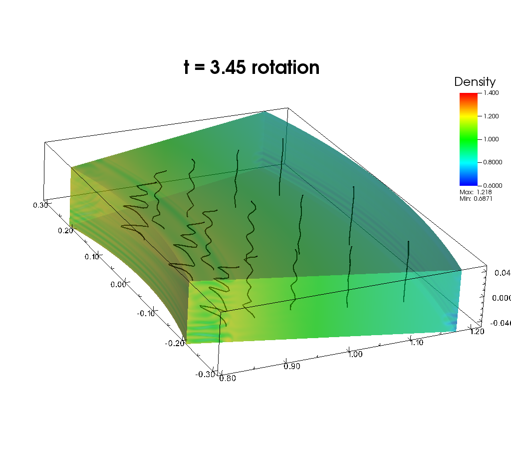
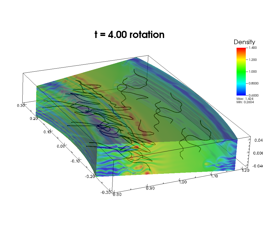
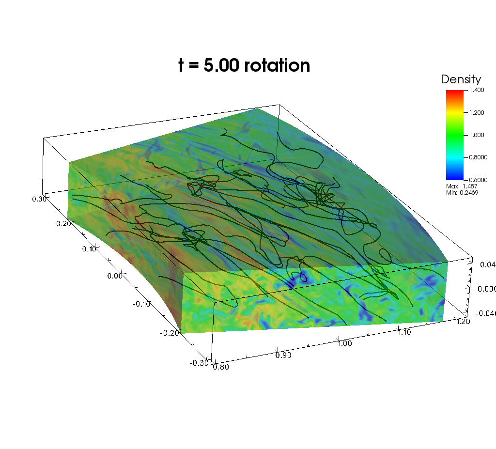
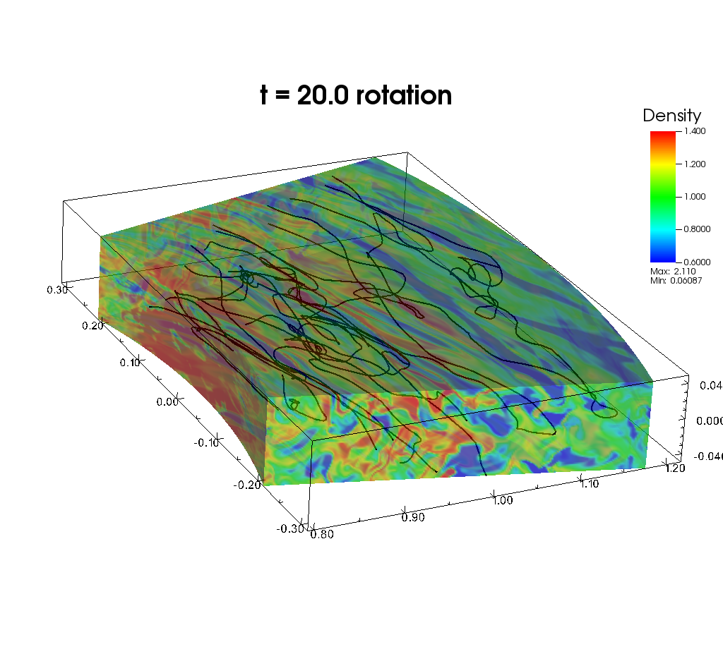
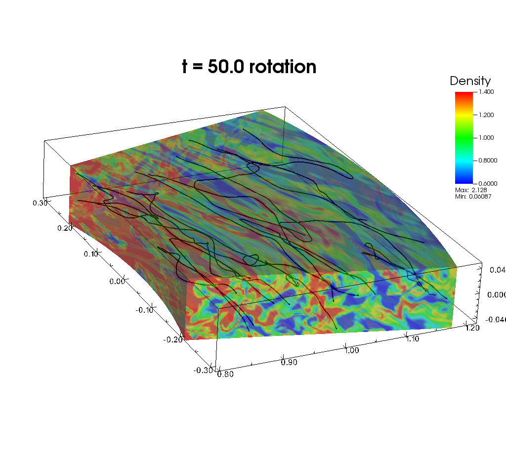
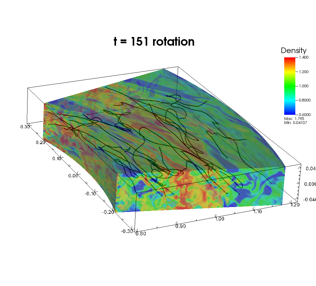
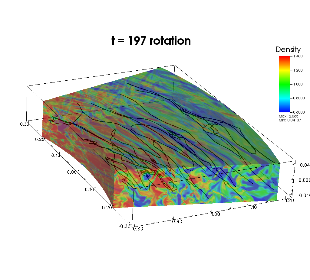
Figure 1: Time evolution of the cylindrical case. Colors denote density and black lines indicate magnetic field lines. Movie is available at http://ea.c.u-tokyo.ac.jp/astro/Members/stakeru/research/cylshbx.

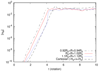
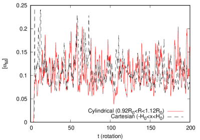
Figure 2: Time evolution of $\alpha_{\rm M}$. The left panel focuses on the early times of $t<10(2\pi/\Omega_{\rm K,0})$. The black dot-dashed, red solid, and blue dotted lines respectively indicate the time evolution of inner ($0.92R_{0}<R<0.94R_{0}$), intermediate ($R_{0}<R<1.02R_{0}$), and outer ($1.1R_{0}<R<1.12R_{0}$) regions of the cylindrical shearing box. The right panel presents the time evolution of a broader region of $0.92R_{0}<R<1.12R_{0}$ of the cylindrical shearing box by the red solid line until the end of the simulations at $t=200(2\pi/\Omega_{\rm K,0})$. In both panels, the result of the Cartesian case averaged in the region of $-H_{0}<x<H_{0}$ is also represented by black dashed lines for comparison.

Figure 1 shows 3D snapshots of the cylindrical case at eight different time slices. The evolution at the early times ($=3-4$ rotations) exhibits that the MRI starts to grow from inner locations, because the growth rate is $\approx\frac{3}{4}\Omega_{\rm K}\propto R^{-3/2}$ (Balbus & Hawley, 1991) in this nearly Keplerian rotation condition. At $t=3.45$ rotations, the field lines in $R<R_{0}$ show channel-mode patterns, although the outer field lines are still almost straight. At the slightly later times at $t=4$ rotations, the inner region is already in the nonlinear regime, while the outer region is still in the linear growth stage of MRI. Inspecting these two panels, one can also recognize the radial dependence of $\lambda_{\rm max,init}(\propto R)$ in eq.(38).

The MRI initially excites radial magnetic field from the vertical field as shown in these two panels. Later on the toroidal magnetic field is amplified from $B_{R}$ by differential rotation. As a result, $B_{\phi}$ dominates the poloidal components at and after $t=5$ rotations. After $t\gtrsim 20$ rotations, the magnetic field is amplified to the saturated state.

The lower four panels show density perturbations are also excited in the nonlinear saturation stage. At $t=50$ and 197 rotations, the density fluctuations are larger than those at other times. At $t=151$ rotations, a density bump is formed around $R\approx R_{0}$ (see also Figure 3), although the overall density fluctuations in the entire box is moderately smaller.

Figure 2 presents the time evolution of the dimensionless volume averaged $R\phi$ component of the Maxwell stress,

$$[\alpha_{\rm M}]_{R_{1}}^{R_{2}}=\frac{-\int_{R_{1}}^{R_{2}}RdR\langle B_{R}B_{\phi}/4\pi\rangle}{\int_{R_{1}}^{R_{2}}RdR\langle\rho c_{\rm s}^{2}\rangle},$$ (39)

where from now on we define $\langle A\rangle$ as the $\phi$ and $z$ integrated average of some variable, $A$, at $R$

$$\langle A\rangle\equiv\frac{\int_{z_{-}}^{z_{+}}\int_{\phi_{-}}^{\phi_{+}}d\phi dzA}{\int_{z_{-}}^{z_{+}}\int_{\phi_{-}}^{\phi_{+}}d\phi dz}.$$ (40)

By changing $R_{1}$ and $R_{2}$ in eq.(39), we compare $\alpha_{\rm M}$ in different regions; we set an inner region of $0.92R_{0}<R<0.94R_{0}$, a middle region of $1R_{0}<R<1.02R_{0}$, and an outer region of $1.1R_{0}<R<1.12R_{0}$.

The left panel shows the growth of $\alpha_{\rm M}$ in these three different regions of the cylindrical shearing box at the early time before 10 rotations, in comparison to the result of the Cartesian box. The increase of $\alpha_{\rm M}$ is faster at smaller $R$, because the growth rate of MRI is roughly proportional to $\Omega_{\rm K}\propto R^{-3/2}$. The slope of the Cartesian case coincides with the slope of the middle region ($R_{0}<R<1.02R_{0}$) of the cylindrical case, as expected. However, the onset time of the Cartesian case is slightly later. We do not know the exact reason of this time difference; it is probably because of the effect of curvature (Latter et al., 2015).

After $t\gtrsim 4$ rotations, the amplification of the magnetic field almost saturates. The right panel compares the cylindrical and Cartesian cases until the end of the simulation ($=200$ rotations). For direct comparison, we picked regions with the same radial extent of $2H_{0}$, $0.92R_{0}<R<1.12R_{0}$ and $-H_{0}<x<H_{0}$, respectively. Although the region of the radial box is $0.91R_{0}<R<1.11R_{0}$ if we choose the same grid number across $R=R_{0}$, we slightly shift it outward to avoid the effect of the inner boundary (see Subsection 5.2). While both cases exhibit intermittent behavior, the time averaged values during $50-200(2\pi/\Omega_{\rm K,0})$ are quite similar; the cylindrical case gives $\alpha_{\rm M}=0.106$ and the Cartesian case gives $\alpha_{\rm M}=0.109$.

4.2 Radial Distribution

We examine time, $\phi$, and $z$ averaged radial profiles of various physical quantities in this subsection. The $\phi$ and $z$ averages are taken by eq.(40). We take the time average from $t=50$ to 200 rotations, unless otherwise noted.

4.2.1 $\rho$ & $v_{\phi}$

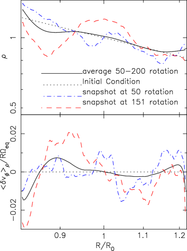
Figure 3: Comparison of radial profiles of $\phi$ and $z$ averaged density (upper panel) and dimensionless shift of azimuthal velocity from the initial equilibrium distribution ($\delta v_{\phi}/R\Omega_{\rm eq}$; lower panel) at different times. Black dotted and black solid lines indicate the initial condition and the time average from 50 – 200 rotations, respectively. Blue dash-dotted and red dashed lines denote the snapshots at 50 rotations and 151 rotations, respectively, where the corresponding 3D snapshots are shown in Figure 1.

The upper panel of Figure 3 compares radial density profiles at different times. The time-averaged distribution (black solid line) shows that the initial profile (black dotted line) is almost preserved. The deviations from the initial condition is larger near the inner and outer boundaries. The gas slightly piles up near both boundaries and the density there increases about 10% from the initial value because of boundary effects.

Snapshots at $t=50$ (blue dash dotted line) and 151 (red solid line) rotations illustrates that the density distribution considerably varies with time. At $t=151$ rotations, one can see a density bump with the density enhancement by $\approx 15\%$ from the initial condition near $R\approx R_{0}$, which can be also seen in the 3D snapshot (Figure 1). This density enhancement is a transiently formed zonal flow, which was also observed in Cartesian shearing box simulations (Johansen et al., 2009; Simon et al., 2018).

The lower panel of Figure 3 shows how the initial equilibrium rotational profile is perturbed with time. We present density weighted $\delta v_{\phi}$ (eq.12),

$$\langle\delta v_{\phi}\rangle_{\rho}\equiv\frac{\langle\rho\delta v_{\phi}\rangle}{\langle\rho\rangle},$$ (41)

which is further normalized by the equilibrium rotational velocity measured in the laboratory frame.

The time-averaged profile (solid line) shows that the dimensionless $\delta v_{\phi}$ is kept small with $<1.5\%$ in the entire region, while the deviations are larger near the inner and outer boundaries where the slope of $\langle\rho\rangle$ changes from the initial condition. A steeper decrease of gas pressure with $R$ reduces the rotational velocity near the inner boundary; a smaller contribution from the centrifugal force is sufficient to balance with the inward gravity, because of the larger outward pressure gradient force. Since in our simulation we assume the locally isothermal condition, the pressure gradient force is modified only by the change of a density gradient.

Comparing the $\delta v_{\phi}$ and $\rho$ profiles, one can find that negative (positive) $\delta v_{\phi}$ corresponds to the steeper (shallower) slope of density. While the two snapshots of $\delta v_{\phi}$ roughly show the similar tendency, the detailed structures do not exactly follow it. This is because the radial force balance is not always satisfied when the gas moves radially in a time-dependent manner.

4.2.2 Magnetic Field

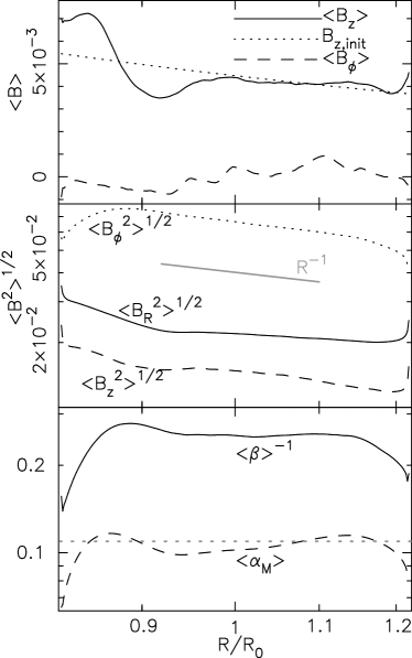
Figure 4: Radial distributions of various time-averaged quantities concerning the magnetic field. Top: The $z$ (solid) and $\phi$ (dashed) components of the net magnetic flux density. The initial profile of $B_{z}$ is also plotted for comparison. Note that $\langle B_{R}\rangle$ is not shown because it is strictly 0 by the conservation law of eq.(27). Middle: Comparison of the $R$ (solid), $\phi$ (dotted), and $z$ (dashed) components of the root-mean-squared $B$. Bottom: The inverse of plasma $\langle\beta\rangle$ (solid) and the $R\phi$ component of the Maxwell stress, $\langle\alpha_{\rm M}\rangle$ (dashed). The gray dotted lines are those from the $-H_{0}<x<H_{0}$ region of the Cartesian shearing box.

Figure 4 presents various quantities of the magnetic field. The top panel compares the radial profile of net magnetic flux, $\langle B\rangle$, to the initial strength of the vertical magnetic field. We note that $\langle B_{R}\rangle$ is kept to 0 within the accuracy of a round-off error in our simulation because of the conservation law of eq.(27), and therefore we only present $\langle B_{\phi}\rangle$ (dashed) and $\langle B_{z}\rangle$ (solid).

This panel indicates that the initial profile of $B_{z}$ is roughly preserved, although moderate pileups of $B_{z}$ are seen near both boundaries, which are also formed by the influence of the radial boundaries, as discussed in the density distribution (Figure 3).

$\langle B_{\phi}\rangle$ shows that the initial condition ($=0$) is also almost conserved. We would like to note that the integrated $\int_{R_{-}}^{R_{+}}dRR\langle B_{\phi}\rangle$ in the box is strictly $0$ in our simulation by the conservation law of eq.(27) and the periodic condition at the $\phi$ boundaries.

The middle panel of Figure 4 presents the three components of the root-mean-squared magnetic field, $\sqrt{\langle B^{2}\rangle}$, which is generally much larger than $\langle B\rangle$ by the contribution from the turbulent component. The toroidal component dominates the poloidal ($R$ & $z$) components because the differential rotation winds up and amplifies $B_{\phi}$, which is consistent with results obtained in local Cartesian shearing box simulations (e.g., Hawley et al., 1995; Sano et al., 2004; Davis et al., 2010) and global simulations (e.g., Armitage, 1998; Hawley, 2000; Suzuki & Inutsuka, 2014). The relative values in units of magnetic energy is $B_{R}^{2}:B_{z}^{2}:B_{\phi}^{2}\approx 2:1:10-15$ except in the regions near both boundaries.

The middle panel also shows that $\sqrt{\langle B_{\phi}^{2}\rangle}\propto 1/R$ in $0.9R_{0}\lesssim R\lesssim 1.15R$. This trend is obtained in previous global simulations (Flock et al., 2011; Suzuki & Inutsuka, 2014), which is anticipated from the radial force balance between magnetic pressure and hoop stress,

$$-\frac{1}{R^{2}}\frac{\partial}{\partial R}\left(R^{2}\frac{B_{\phi}^{2}}{8\pi}\right)=-\frac{\partial}{\partial R}\left(\frac{B_{\phi}^{2}}{8\pi}\right)-\frac{B_{\phi}^{2}}{4\pi R}\approx 0.$$ (42)

Near the radial boundaries, $\sqrt{\langle B_{\phi}^{2}\rangle}$ is weaker than the strength expected from this trend. This is because the differential rotation is weaker there, which corresponds to $\frac{\partial\delta v_{\phi}}{\partial R}>0$ in Figure 3, and therefore the amplification of magnetic field is suppressed. The poloidal components, which show a roughly similar radial dependence to that of $B_{\phi}$, are basically controlled by the dominant toroidal component, whereas they are also affected by the radial boundaries.

The bottom panel of Figure 4 presents $\alpha_{\rm M}$ (dashed line) and the inverse of a plasma $\beta$ value (solid line), which is defined by the ratio of gas pressure to magnetic pressure. Again, both quantities are averaged over the $\phi$ and $z$ components:

$$\langle\alpha_{\rm M}\rangle=\frac{-\langle B_{R}B_{\phi}/4\pi\rangle}{\langle\rho c_{\rm s}^{2}\rangle},$$ (43)

and

$$\langle\beta\rangle^{-1}\equiv\frac{(\langle B_{R}^{2}+B_{\phi}^{2}+B_{z}^{2})/8\pi\rangle}{\langle\rho c_{\rm s}^{2}\rangle}.$$ (44)

The results of the Cartesian shearing box are also plotted (gray dotted lines) for comparison. Both $\langle\beta\rangle^{-1}$ and $\langle\alpha_{\rm M}\rangle$ show almost flat dependence on $R$ except in the regions near the boundaries, and their values also agree with those of the Cartesian case within 10% difference. $\langle\beta\rangle^{-1}\approx 0.25$ in the flat region ($0.93R_{0}<R<1.15R_{0}$), which indicates that the magnetic energy ($\propto B^{2}$) is amplified by 250 times from the initial condition, $\beta_{z,{\rm init}}^{-1}=10^{-3}$ (eq.34).

The magnetic pressure, which is dominated by $B_{\phi}^{2}/8\pi$, is proportional to $R^{-2}$, as shown in the middle panel. This dependence is the same as that of the gas pressure, since $\rho\propto R^{-1}$ is adopted at the radial shearing periodic boundaries (eq.30) and $c_{\rm s}^{2}\propto R^{-1}$ is fixed in our locally isothermal assumption. Therefore, the $R^{-2}$ dependences of both numerator and denominator of eq.(44) are canceled out so that $\langle\beta\rangle^{-1}$ is nearly a constant on $R$.

$\langle\alpha_{\rm M}\rangle$ is also a nearly constant but slightly increases with $R$ in the middle region that is not affected by the boundaries. This weak dependence is important in the transport of angular momentum and consequent mass accretion, which is discussed in the next subsection.

4.2.3 Angular Momentum & Accretion

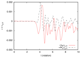
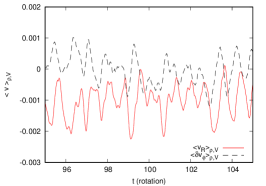
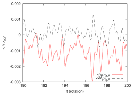
Figure 5: Time evolution of the density weighted and volume averaged $v_{R}$ (solid red lines) and $\delta v_{\phi}$ (black dashed lines). The left, middle, and right panels respectively show the initial, intermediate, and final 10 rotations of the simulation.

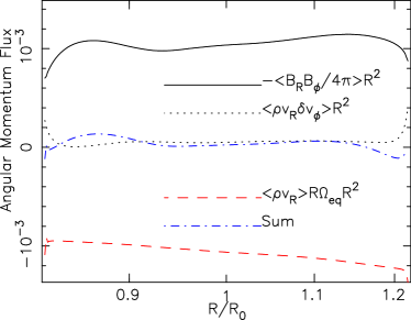
Figure 6: Comparison of different components of time-averaged angular momentum fluxes. The black solid, black dotted, and red dashed lines respectively show the angular momentum fluxes carried by the $R\phi$ component of the Maxwell stress, the turbulent Reynolds stress, and the net mass accretion. The blue dash-dotted line represents the sum of these three components.

A great advantage of our cylindrical shearing box approach to the Cartesian shearing box setup is that we can handle radial mass accretion directly. In order to realize this, we do not impose a shearing periodic constraint on the total angular momentum at the radial boundaries but instead constrain the turbulent part (see eq.(14) in Subsection 2.2 & Appendix C). The total angular momentum in the simulation box is not conserved, and mass accretion or decretion can be automatically induced by the loss or gain of angular momentum. In other words, we liberate the center of mass in the box from a fixed origin and test whether time-steady mass accretion is actually achieved by the outward transport of angular momentum via excited MHD turbulence.

Let us examine the time evolution of the radial and angular momentums in the simulation box. Figure 5 presents the density weighted and volume averaged horizontal velocities, $\langle v_{R}\rangle_{\rho,V}$ and $\langle\delta v_{\phi}\rangle_{\rho,V}$, where $\langle v\rangle_{\rho,V}\equiv[\rho v]_{{}_{V}}/[\rho]_{{}_{V}}$. From eqs.(24) and (25) we can derive the solutions that represent epicyclic oscillations with an arbitrary velocity amplitude, $a$:

$$\langle\delta v_{\phi}\rangle_{\rho,V}\approx a\sin\left(\Omega_{\rm eq,0}t+\delta\right)$$ (45)

$$\langle v_{R}\rangle_{\rho,V}\approx 2a\sin\left(\Omega_{\rm eq,0}t+\delta-\frac{\pi}{2}\right),$$ (46)

where $\delta$ is a phase shift. These solutions show that the phase of $\langle v_{R}\rangle_{\rho,V}$ is delayed by $\pi/2$ from that of $\langle\delta v_{\phi}\rangle_{\rho,V}$ and the amplitude of $\langle v_{R}\rangle_{\rho,V}$ is twice that of $\langle\delta v_{\phi}\rangle_{\rho,V}$

Readers can recognize that the oscillatory behavior of the horizontal velocities in Figure 5 roughly follow the characteristics of these epicyclic oscillations, although it is considerably perturbed from time to time by the magnetic field and the curvature effects that are not considered in the solutions of eqs. (45) and (46). The left panel of Figure 5 shows that the simulation box starts to oscillate at $t\gtrsim 3$ rotations when the magnetic field is amplified by the MRI. While $\langle\delta v_{\phi}\rangle_{\rho,V}$ oscillates around 0, the center of the oscillation of $\langle v_{R}\rangle_{\rho,V}$ slowly shifts downward; the mass accretion is gradually induced.

In the middle (95-105 rotations) and right (190-200 rotations) panels, $\langle v_{R}\rangle_{\rho,V}$ does not decrease monotonically but it oscillates roughly around $\approx 0.001$. This indicates that the mass accretion occurs in a quasi-steady manner, if we take a time average covering the duration of $\gtrsim 10$ rotations. On the other hand, the oscillation of $\langle\delta v_{\phi}\rangle_{\rho,V}$ is still kept around $\approx 0$ at later times. This clearly shows that the total angular momentum is almost conserved for the long-time average. We can conclude that, by utilizing the shearing variable of the angular momentum, $S_{\rm mom,\phi}$, (eq.14), the time-steady mass accretion can be realized while keeping the angular momentum in the box conserved, as we aimed in Subsection 2.2.

Next, we inspect the radial profile of different components of angular momentum fluxes when the mass accretes in a quasi-steady manner. Taking the $\phi$ and $z$ integrated average under the periodic boundary condition and assuming the steady-state condition, $\partial_{t}\cdots=0$, we can obtain an equation that describes the balance of angular momentum fluxes in the laboratory frame ( see eq.58) as

$$\frac{\partial}{\partial R}\left[R^{2}\left(\langle\rho v_{R}\rangle R\Omega_{\rm eq}+\langle\rho v_{R}\delta v_{\phi}\rangle-\frac{\langle B_{R}B_{\phi}\rangle}{4\pi}\right)\right]=0,$$ (47)

where the first term indicates the angular momentum flux carried by net radial flows, the second term is that by the turbulent Reynolds stress, and the third term is that by the Maxwell stress. We note that in the Cartesian shearing box approach, mass accretion rate, $\dot{M}$, is estimated from the second and third terms by using this equation,

$$\dot{M}\equiv-2\pi\int dzR\rho v_{R}\approx-\frac{2\pi}{\Omega_{\rm K}}\int dz\left\langle\rho v_{R}\delta v_{\phi}-\frac{B_{R}B_{\phi}}{4\pi}\right\rangle,$$ (48)

even though net $\langle v_{R}\rangle=0$. Our cylindrical shearing box can directly test the justification of this conventional approach.

Figure 6 compares the three terms of eq.(47), where the time averages are again taken from 50 to 200 rotations. The outward transport of angular momentum is mainly done by the Maxwell stress (black solid). The turbulent Reynolds stress (black dotted) also transports angular momentum outward, however its contribution is $\lesssim 1/10$ times smaller than that from the Maxwell stress in most of the simulation region. On the other hand, the sign of the accretion term is negative, which indicates that the angular momentum is carried inward by the net mass accretion.

The sum of these three terms (blue dash-dotted line) is nearly 0; the balance between the outward transport by the MHD turbulence and the inward transport by the mass accretion is almost satisfied, and the total angular momentum is conserved in a self-regulating manner after the magnetic field is amplified to the saturated state, even though we do not impose a constraint on the total angular momentum.

From the conservation law of eq.(9), our simulation gives $\langle\rho v_{R}R\rangle=$ const. We adopt the nearly Keplerian rotational velocity for the equilibrium state, which roughly gives $\Omega_{\rm eq}\propto R^{-3/2}$. These relations leads to the $R$ scaling of the first term of eq.(47) as $R^{2}\langle\rho v_{R}\rangle R\Omega_{\rm eq}\propto R^{1/2}$. The weak radial dependence of the accretion term in Figure 6 reflects this $R^{1/2}$ scaling. The Maxwell stress also shows the same dependence of $-\langle B_{R}B_{\phi}/4\pi\rangle R^{2}\propto R^{1/2}$ to balance with the accretion term. This dependence is consistent with $\langle\alpha_{\rm M}\rangle\propto R^{1/2}$ in Figure 4, and further implies that the (dimensional) turbulent viscosity, $\nu_{\rm M}$, of the Maxwell stress has the relation of $\nu_{\rm M}\approx\langle\alpha_{\rm M}\rangle c_{\rm s}H\approx\langle\alpha_{\rm M}\rangle c_{\rm s}^{2}/\Omega_{K}\propto R$.

4.2.4 Mass Accretion and Radial Transport of $B_{z}$

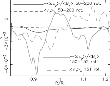
Figure 7: Comparison of the radial flows of gas ($\langle v_{R}\rangle_{\rho}$; dashed lines) and vertical magnetic field ($\langle v_{R}\rangle_{B_{z}}=\langle cE_{\phi}\rangle/\langle B_{z}\rangle$; solid lines). The thin black lines are the time average from 50-200 rotations, and the gray lines are the snapshots at 151 rotations, where we take the average of $\pm$ one rotations for $\langle v_{R}\rangle_{B_{z}}$.

In the previous subsection we have discussed the mass accretion from a viewpoint of the angular momentum balance. In this subsection, we further inspect radial flows of not only mass but also vertical magnetic field. As discussed in Suzuki & Inutsuka (2014), the radial velocity of the gas and that of the vertical magnetic fields do not generally coincide, even if the ideal MHD condition is considered, because of the turbulent diffusion of magnetic fields. The radial flow of $B_{z}$ determines the pileup or diffusion of the poloidal magnetic field in a disk, and consequently controls the long-time evolution of the large-scale magnetic field (Lubow et al., 1994; Rothstein & Lovelace, 2008; Guilet & Ogilvie, 2012; Okuzumi et al., 2014; Takeuchi & Okuzumi, 2014).

The radial velocity of gas is taken from the density weighted average,

$$\langle v_{R}\rangle_{\rho}=\frac{\langle\rho v_{R}\rangle}{\langle\rho\rangle},$$ (49)

where the subscript $\rho$ is put to explicitly show gas flow. For the radial velocity of $B_{z}$, we introduce

$$\langle v_{R}\rangle_{B_{z}}=-\frac{\langle cE_{\phi}\rangle}{\langle B_{z}\rangle}=\frac{\langle v_{R}B_{z}-v_{z}B_{R}\rangle}{\langle B_{z}\rangle},$$ (50)

which is expected from the $z$ component of the induction equation (eq.3). Taking the $\phi$ and $z$ integration of the equation that describes the time variation of $B_{z}$, we get

$$\frac{\partial\langle B_{z}\rangle}{\partial t}+\frac{1}{R}\frac{\partial}{\partial R}\left[R(-\langle cE_{\phi}\rangle)\right]=0.$$ (51)

The form of eq.(51) is essentially an equation of continuity for $\langle B_{z}\rangle$, and therefore, we use eq.(50) to follow the radial motion of $\langle B_{z}\rangle$.

Figure 7 compares $\langle v_{R}\rangle_{\rho}$ (dashed) and $\langle v_{R}\rangle_{B_{z}}$ (solid). The time averaged gas flow (thin black dashed line) shows the gas accretes inward with a constant $\langle v_{R}\rangle_{\rho}$, which is consistent with eq.(31) and the discussion in Sub-subsection 4.2.3.

The time-averaged radial velocity of the vertical magnetic field also shows a nearly constant $\langle v_{R}\rangle_{B_{z}}$. However, the inward velocity is slightly faster, $\langle v_{R}\rangle_{B_{z}}<\langle v_{R}\rangle_{\rho}(<0)$, in most of the region except near the inner boundary, which indicates that the vertical magnetic flux drifts inward through the gas. As discussed above, the magnetic field is not strictly frozen into the gas, even though the ideal MHD condition is imposed on the simulation. The inward velocity of $B_{z}$ is decelerated from $R=0.9R_{0}$ to $0.85R_{0}$, which leads to the pileup of the vertical magnetic flux, as discussed in Figure 4.

The snapshot profiles of $\langle v_{R}\rangle_{\rho}$ and $\langle v_{R}\rangle_{B_{z}}$ at $t=151$ rotations are also plotted in Figure 7. As for $\langle v_{R}\rangle_{B_{z}}$, we take the average from $t=150$ to 152 rotations, because the pure snapshot gives spuriously huge values at locations where $\langle B_{z}\rangle$ is occasionally $\approx 0$.

Both $\langle v_{R}\rangle_{\rho}$ and $\langle v_{R}\rangle_{B_{z}}$ indicate that the mass accretion and the inward transport of magnetic flux do not occur in a time-steady manner. The direction of the gas flow is inward in the inner side ($R\lesssim R_{0}$) and outward in the outer side ($R\gtrsim R_{0}$) at $t=151$ rotations because diverging flows are excited from the density bump that is formed at this time (Figures 1 & 3).

The snapshot of $\langle v_{R}\rangle_{B_{z}}$ (gray solid line) largely deviates from that of $\langle v_{R}\rangle_{\rho}$ (gray dashed line); the radial motion of $B_{z}$ drifts from the accreting gas because of turbulent diffusion and reconnection (Lazarian & Vishniac, 1999).

5 Discussion

5.1 Treatment of Radial Boundaries

After the simulation starts from the initial condition of $v_{R}=\mbox{\boldmath${0}$}$, mass accretion is gradually induced by the excited MHD turbulence that transports angular momentum outward (Figure 5). We did not impose any constraint on the mass accretion rate or the angular momentum transport rate. The mass accretion rate is determined by the balance between the angular momentum fluxes from mass accretion and MHD turbulence in a self-consistent and self-regulating manner. Each component of the time-averaged radial angular momentum flux shows a smooth and monotonic profile in $R$ (Figure 6). The treatment of the radial boundary condition works well at least for handling the time-averaged properties of the mass accretion.

However, there are issues concerning the boundary treatment that should be addressed in future work. The first point arises from the difference between $\Omega_{\rm eq,+}$ and $\Omega_{\rm eq,-}$ at the $R_{\pm}$ boundaries. At the linear stage of the MRI, the magnetic field grows first at the inner boundary because the growth time ($\propto\Omega_{\rm eq}$) is shortest there. A part of the amplified magnetic field at the inner boundary is transported to the outer boundary and into the simulation domain because of the shearing periodic condition (Figure 1), which does not occur in realistic accretion disks. For this reason, we have to be careful when we focus on specific phenomena, such as individual channel flows, near the radial boundaries. On the other hand, we expect that the radial boundary treatment gives reasonable time-averaged properties, provided that the appropriate shearing variables, $S$, are adopted (Subsection 2.2).

Another possible concern is the propagation of waves across the radial boundary, which is also related to the difference between $\Omega_{\rm eq,+}$ and $\Omega_{\rm eq,-}$. We can expand the basic MHD equations (eqs.1–4) into the mean and fluctuating components, and MHD waves are derived from the latter component. The current formulation using the shearing variables focuses only on the mean component and does not take special care of the fluctuating component. Therefore, waves that propagate across the radial boundary could suffer partial reflection. The treatment of the fluctuating component should be done as a next step.

5.2 Zonal Flows

The radial distribution of the density exhibits bumps and dips. Although the amplitudes of the radial density variations are not so large, they are not erased even for the time average over 50 – 200 rotations (Figure 3). Because of the bumpy profile of the density and, accordingly, the pressure, the azimuthal velocity also deviates from the equilibrium value with $\delta v_{\phi}<0$ ($>0$) in regions with a steeper (shallower) density gradient than the equilibrium gradient. As a result, the differential rotation is not constant in $R$. The toroidal magnetic field is more amplified in the regions with stronger differential rotation, $\frac{\partial\delta v_{\phi}}{\partial R}<0$. As a result, the unsigned toroidal magnetic field, $\sqrt{B_{\phi}^{2}}$, is not a monotonically decreasing function of $R$ but shows a peak at $R\approx 0.88R_{0}$, as discussed in Sub-subsection 4.2.2.

Although the bumpy density structures, or zonal flows, are created physically (Johansen et al., 2009), they may be affected by the radial boundaries because the deviation of $\langle\delta v_{\phi}\rangle$ from 0 is larger near both radial boundaries. In particular, it is more prominent near the inner boundary because the curvature effect ($\propto 1/R$) is more severe there. The partial reflection of propagating waves at the radial boundary (Subsection 5.1) may cause the bumpy density structure.

In addition, the numerical implementation may cause the bumpy density structure. We adopt the CT scheme to update the magnetic field. The locations of the three components of the magnetic field are different from that of the other physical variables. Therefore, interpolation is required to use the shearing variables with magnetic fields, which causes truncation errors and numerical diffusion. Our specific implementation method is described in Appendix C. Although we carefully chose the interpolation method after much trial and error, it still may not be a perfect one. More elaborate and innovative methods will be explored in future work.

5.3 Radial Dependences and Shearing Variables

In this paper we presented one simulation with a single set of radial dependences for the density, the temperature, and the vertical magnetic field strength. The power-law index of the density, $q_{\rho}=1$, is required from the shearing conditions for $S_{\rm mass}$ (eq.9) and $S_{{\rm mom},r}$ (eq.57). The power-law index of the temperature, $q_{T}=1$, is chosen to give $c_{\rm s}\propto R^{-1/2}$, which is the same scaling as that of the equilibrium rotation velocity. The power-law index of the initial net vertical magnetic flux, $q_{B}=1$, is regulated from the adopted $q_{\rho}$ and $q_{T}$ to give a constant $\beta_{z,{\rm init}}$.

In general, however, the radial dependences are determined independently of each other. Therefore, it is worth pursuing cases with different sets of power-law indices to study various types of accretion disks, which we plan to tackle in our future studies.

Among the three power-law indices, $q_{\rho}$ needs to be treated carefully. The adopted $q_{\rho}=1$ is consistent with the conservation of mass via $S_{\rm mass}$ (eq.9) and radial momentum via $S_{{\rm mom},r}$ (eq.10). When a different $q_{\rho}$ is adopted, we cannot satisfy the shearing variables of both $S_{\rm mass}$ and $S_{{\rm mom},r}$ simultaneously, and have to dismiss either one of then.

It is better to keep $S_{\rm mass}$ rather than $S_{{\rm mom},r}$, because even in the present formulation the radial momentum is conserved only in an approximate sense (Subsection 2.2). However, in this case the radial dynamical pressures, $(\rho v_{R}^{2}R)_{\pm}$, at the $R_{\pm}$ boundaries are not balanced, and hence, the simulation box will be accelerated to the $+$ or $-R$ direction. A prescription to prevent this systematic acceleration must take into account the magnetic terms (see eq.57) in $S_{{\rm mom},r}$.

5.4 Future Applications

Although there is room to improve the treatment of the radial shearing boundary (Subsection 5.1), the cylindrical shearing box model has various possible extensions and applications.

5.4.1 Vertical Stratification

A first extension of the cylindrical shearing box framework takes into account the stratification of density by the vertical component of the gravity of a central object.

In recent years, vertical outflows and disk winds have been widely discussed that they play a significant role in the evolution of protoplanetary disks (Ferreira et al., 2006; Suzuki et al., 2016; Takahashi & Muto, 2018), and they are studied in vertically stratified Cartesian shearing box simulations (Suzuki & Inutsuka, 2009; Suzuki et al., 2010; Bai, 2013; Bai & Stone, 2013a; Lesur et al., 2013; Fromang et al., 2013; Riols et al., 2016; Mori et al., 2019). The magnetic centrifugal force often plays an important role in driving disk winds (Blandford & Payne, 1982). In addition to MHD turbulence, magnetocentrifugal acceleration that removes angular momentum from a disk causes the accretion of gas (Pelletier & Pudritz, 1992).

In principle it is quite difficult, and probably impossible, to properly treat the magnetocentrifugal acceleration with the Cartesian shearing box model because of the $\pm x$ symmetry (Section 1). The vertical component of the angular momentum flux is evaluated from the $yz$ component of the Maxwell and Reynolds stresses in Cartesian coordinates. However, the sign of the vertical angular momentum flux is ambiguous because of the $\pm x$ symmetry; it is flipped when the central object is switched from the $-x$ direction to the $+x$ direction.

In contrast, there is no such ambiguity in the sign of the angular momentum flux in the cylindrical approach. The cylindrical shearing box with vertical stratification can properly evaluate the removal rate of angular momentum by magnetocentrifugal driven disk winds.

There are some issues that are not present in the Cartesian shearing box when we include the vertical density stratification in the cylindrical shearing box. The first issue is the radial dependence of the scale height. For example, we presented the case with $H\propto R$, which is derived from $q_{T}=1$. When we apply the radial shearing boundary conditions to a vertically stratified box, the radial dependence of $H$ needs to be taken into account in a consistent way.

Another point is that the equilibrium rotational velocity generally involves vertical shear (see, e.g. Suzuki & Inutsuka, 2014). The gravity of a central object is weaker at higher altitudes. Therefore, rotational velocities are usually slower at higher altitudes for the same $R$, though this can be reversed by the contribution from the pressure gradient force. We note that there is an attempt to consider the vertical shear in the Cartesian shearing box by McNally & Pessah (2015).

5.4.2 Spherical Coordinates

We can extend our framework of the cylindrical shearing box to spherical coordinates in a straightforward manner. When the vertical stratification is taken into account, it is probably better to adopt spherical coordinates rather than cylindrical coordinates, as in the “spherical disks” by Klahr & Bodenheimer (2003), because the disk scale height usually increases with distance from the origin.

5.4.3 Physical Processes

In the presented simulation we solved the ideal MHD equations with a locally isothermal equation of state, which is the simplest setting for demonstrative purposes. It is possible to consider various physical processes in the cylindrical shearing box as is done in Cartesian shearing box simulations.

For example, self-gravity can be included in the momentum equation to study the formation of stars, brown dwarfs, and planets (Gammie, 2001; Hirose & Shi, 2019). To determine realistic temperature distributions in various types of disks, radiative cooling and heating should be considered in the energy equation (Turner et al., 2003; Hirose et al., 2006; Shi et al., 2010; Jiang et al., 2013). If the temperature is not high and the ionization is not sufficient, as expected in protoplanetary disks, the magnetic diffusion by non-ideal MHD effects needs to be taken into account (Sano & Stone, 2002; Bai & Stone, 2013b; Kunz & Lesur, 2013; Mohandas & Pessah, 2017).

5.4.4 Particles

The shearing box model is also a strong tool to study the dynamics of particles in accretion disks.

The energization of non-thermal particles in accretion disks around compact objects has been investigated by particle-in-cell simulations in Cartesian shearing boxes (e.g., Hoshino, 2015; Kunz et al., 2016). One of the severe problems of using the Cartesian box is the existence of unphysical runaway particles; once the gyroradius of a particle exceeds the radial box size, it continuously gains the energy as a result of acceleration (Kimura et al., 2016). Therefore, we cannot determine the maximum energy of the accelerated particles in the Cartesian shearing box model. In reality, however, the acceleration eventually saturates when the gyroradius becomes comparable to the size of the system (Kimura et al., 2019). The cylindrical shearing box approach can handle the saturation of the energy gain because it includes the curvature; the size of the acceleration region is regulated by the curvature radius.

The Cartesian shearing box approach is often adopted to study the dynamics of dust grains in protoplanetary disks (e.g., Carballido et al., 2006; Gressel et al., 2012; Zhu et al., 2015). The pressure gradient force induces the inward drift of dust grains from the background gas (Adachi et al., 1976). While this radial drift can be taken into account in the Cartesian shearing box model as an external force (Johansen et al., 2006), the cylindrical shearing box can consider it in a self-consistent way, which can be a reliable method to understand reasonable pathways for the planet formation (e.g., Kobayashi et al., 2016).

The Cartesian shearing box model also considers larger bodies in protoplanetary disks, such as planetesimals and (proto)planets (Nelson & Papaloizou, 2004; Yang et al., 2009; Muto et al., 2010; Tanigawa et al., 2012). One of the targets of this type of simulations is to understand the migration of (proto)planets. The direction and rate of the migration are primarily determined by the difference between the torques exerted by density waves excited from the inner and outer locations of the planet (Tanaka et al., 2002; Crida & Morbidelli, 2007; Baruteau et al., 2014; Kanagawa et al., 2018). In addition, they are also affected by the radial flow of the background gas (Ogihara et al., 2017). It is quite difficult to quantitatively and directly determine the small difference between the inner and outer torques from the background gas flow in the Cartesian shearing box mainly because of the symmetry with respect to the $\pm x$ directions. In contrast, our cylindrical approach would be a powerful tool to solve this problem.

6 Summary

We developed the basic framework of the cylindrical shearing box, focusing on MHD simulations for accretion disks. We constructed the shearing periodic boundary conditions at the radial boundaries by utilizing the conservation relations of the basic MHD equations. While the cylindrical shearing box is basically a local approach, it also takes into account global effects from the curvature of cylindrical coordinates. One of the great advantages of our treatment is that we can directly capture the net mass accretion, which cannot be handled by the Cartesian shearing box treatment because of the radial symmetry.

We performed the MHD simulation in the unstratified cylindrical shearing box with a moderate resolution that resolves one scale height by 64 grid points. Inward mass flows are naturally induced by the outward flux of angular momentum carried by the MHD turbulence. While the local cylindrical simulation box oscillates quasi-periodically as a result of the epicyclic motion, the total angular momentum averaged over $\gtrsim 10$ rotations is conserved by the balance between the inward angular momentum flux advected by the accreting mass and the outward angular momentum flux by the MHD turbulence. The quasi-time-steady accretion is realized in our cylindrical shearing box simulation. The basic physical properties of the excited MHD turbulence, such as the saturation level of the amplified magnetic fields, are similar to those obtained from the Cartesian shearing box.

While the global effects of curvature are considered, the cylindrical shearing box framework still has the advantage of the local approach that (i) fine-scale phenomena of the turbulence can be resolved by zooming in on a local patch of the accretion disk and (ii) long-time simulations can be performed stably within an acceptable computational time. Related to the point (ii), it took only $\sim$ a day for the presented case with a medium resolution of 64 grids per $H_{0}$ (Table 1) to run up to 200 rotations on a standard parallel computer with 512 CPU cores. It would be possible to perform simulations with a similar resolution up to several thousand rotations within a realistic computational time. This could be quite an efficient tool to study long-time evolution governed by the timescale of diffusion.

It is still not easy to run global simulations for long times ($\sim 10^{3-4}$ dynamical timescales). Global simulations usually cover a large dynamic range from a fast rotating inner region to a slow rotating outer region (e.g., Flock et al., 2011; Suzuki & Inutsuka, 2014). Therefore, in order to follow several thousand rotations at the region of interest, usually located at an intermediate region in the simulation domain, it is necessary to cover larger rotation times at the inner region, which is not realistic with the current computational resources.

There is still room to improve the numerical implementation of the radial shearing boundary condition, in particular for the treatment of propagating waves. As discussed in Section 5, the cylindrical shearing box framework has various applications, which are open to future works by all those who are interested.

Numerical computations were carried out on Cray XC40 at YITP, Kyoto University, and Cray XC50 at Center for Computational Astrophysics, National Astronomical Observatory of Japan. We thank Geoffroy Lesur, James Stone, and Charles Gammie for valuable and critical comments on an earlier version of the draft. The authors thank the referee for many constructive comments. This work was supported by Grants-in-Aid for Scientific Research from the MEXT of Japan, 17H01105.

Appendix A Treatment of External Forces

The radial component of the momentum equation, eq.(2), is written as

$$\frac{\partial v_{R}}{\partial t}+v_{R}\frac{\partial v_{R}}{\partial R}+\frac{v_{\phi}}{R}\frac{\partial v_{R}}{\partial\phi}+v_{z}\frac{\partial v_{R}}{\partial z}-\frac{v_{\phi}^{2}}{R}=-\frac{1}{\rho}\frac{\partial}{\partial R}\left(p+\frac{B_{\phi}^{2}+B_{z}^{2}}{8\pi}\right)$$

$$+\frac{B_{\phi}}{4\pi\rho R}\frac{\partial B_{R}}{\partial\phi}+\frac{B_{z}}{4\pi\rho}\frac{\partial B_{R}}{\partial z}-\frac{B_{\phi}^{2}}{4\pi\rho R}-\frac{GM_{\star}}{R^{2}}+R\Omega_{\rm eq,0}^{2}+2\Omega_{\rm eq,0}v_{\phi}.$$ (52)

The mutual subtraction of the external forces and the curvature term ($v_{\phi}^{2}/R$) causes the numerical cancellation of significant digits. Therefore, it is better to consider the deviation from the equilibrium profile. In the equilibrium state, the radial force balance

$$F_{\rm eq}\equiv\frac{v_{\phi,{\rm eq}}^{2}}{R}-\frac{1}{\rho_{\rm eq}}\frac{\partial p_{\rm eq}}{\partial R}-\frac{GM_{\star}}{R^{2}}+R\Omega_{\rm eq,0}^{2}+2\Omega_{\rm eq,0}v_{\phi,{\rm eq}}=0$$ (53)

is satisfied, where

$$-\frac{1}{\rho_{\rm eq}}\frac{\partial p_{\rm eq}}{\partial R}=(q_{\rho}+q_{T})\frac{c_{\rm s,0}^{2}}{R}\left(\frac{R}{R_{0}}\right)^{-q_{T}}.$$ (54)

Substituting eq.(53) into eq.(52), we obtain

$$\frac{\partial v_{R}}{\partial t}+v_{R}\frac{\partial v_{R}}{\partial R}+\frac{v_{\phi}}{R}\frac{\partial v_{R}}{\partial\phi}+v_{z}\frac{\partial v_{R}}{\partial z}=-\frac{1}{\rho}\frac{\partial}{\partial R}\left(p+\frac{B_{\phi}^{2}+B_{z}^{2}}{8\pi}\right)$$

$$+\frac{B_{\phi}}{4\pi\rho R}\frac{\partial B_{R}}{\partial\phi}+\frac{B_{z}}{4\pi\rho}\frac{\partial B_{R}}{\partial z}-\frac{B_{\phi}^{2}}{4\pi\rho R}+2\left(\Omega_{\rm eq,0}+\frac{v_{\phi,{\rm eq}}}{R}\right)\delta v_{\phi}+\frac{\delta v_{\phi}^{2}}{R}-(q_{\rho}+q_{T})\frac{c_{\rm s,0}^{2}}{R}\left(\frac{R}{R_{0}}\right)^{-q_{T}}.$$ (55)

We use this expression with $\delta v_{\phi}$ for updating $v_{R}$ to reduce numerical errors.

Appendix B Formulae

B.1 Basic Equations in the Rest Frame

We summarize basic equations in conservative forms in the rest frame. The $R$-derivatives of the following equations are used for the shearing variables presented in Subsection 2.2.

The mass conservation is expressed as

$$\frac{\partial\rho}{\partial t}+\frac{1}{R}\frac{\partial}{\partial R}(\rho u_{R}R)+\frac{1}{R}\frac{\partial}{\partial\phi}(\rho u_{\phi})+\frac{\partial}{\partial z}(\rho u_{z})=0.$$ (56)

The radial component of momentum flux evolves as

$$\frac{\partial}{\partial t}(\rho u_{R})+\frac{1}{R}\frac{\partial}{\partial R}(\rho u_{R}^{2}R)+\frac{1}{R}\frac{\partial}{\partial\phi}(\rho u_{R}u_{\phi})+\frac{\partial}{\partial z}(\rho u_{R}u_{z})=\rho\frac{u_{\phi}^{2}}{R}-\frac{\partial p}{\partial R}-\rho\frac{GM_{\star}}{R^{2}}$$

$$+\frac{1}{R^{2}}\frac{\partial}{\partial R}\left(\frac{B_{R}^{2}R^{2}}{8\pi}\right)-\frac{1}{R^{2}}\frac{\partial}{\partial R}\left(\frac{B_{\phi}^{2}R^{2}}{8\pi}\right)-\frac{\partial}{\partial R}\left(\frac{B_{z}^{2}}{8\pi}\right)+\frac{1}{4\pi}\left[\frac{1}{R}\frac{\partial}{\partial\phi}(B_{R}B_{\phi})+\frac{\partial}{\partial z}(B_{R}B_{z})\right],$$ (57)

where the gravity and a curvature term ($u_{\phi}^{2}/R$) need to be treated as source terms. These two terms and the gas pressure gradient term constitute the main part of radial force balance. Numerical treatment of these terms is described in Appendix A.

The evolution of angular momentum flux is

$$\frac{\partial}{\partial t}(\rho u_{\phi}R)+\frac{1}{R}\frac{\partial}{\partial R}(\rho u_{R}u_{\phi}R^{2})+\frac{1}{R}\frac{\partial}{\partial\phi}(\rho u_{\phi}^{2}R)+\frac{\partial}{\partial z}(\rho u_{\phi}u_{z}R)=-\frac{1}{R}\frac{\partial}{\partial\phi}(pR)$$

$$-\frac{1}{R}\frac{\partial}{\partial\phi}\left[(B_{R}^{2}+B_{z}^{2})R\right]+\frac{1}{R}\frac{\partial}{\partial\phi}\left(\frac{B_{\phi}^{2}R}{8\pi}\right)+\frac{1}{4\pi R}\frac{\partial}{\partial R}(B_{R}B_{\phi}R^{2})+\frac{1}{4\pi}\frac{\partial}{\partial z}(B_{\phi}B_{z}R^{2}).$$ (58)

The vertical component of momentum flux evolves as

$$\frac{\partial}{\partial t}(\rho u_{z})+\frac{1}{R}\frac{\partial}{\partial R}(\rho u_{R}u_{z}R)+\frac{1}{R}\frac{\partial}{\partial\phi}(\rho u_{\phi}u_{z})+\frac{\partial}{\partial z}(\rho u_{z}^{2})=-\frac{\partial}{\partial z}\left(p+\frac{B_{R}^{2}+B_{\phi}^{2}}{8\pi}\right)$$

$$+\frac{\partial}{\partial z}\left(\frac{B_{z}^{2}}{8\pi}\right)+\frac{1}{4\pi R}\frac{\partial}{\partial R}(B_{R}B_{z}R)+\frac{1}{4\pi R}\frac{\partial}{\partial\phi}(B_{\phi}B_{z}).$$ (59)

The three components of the induction equation (eq.3) are

$$\frac{\partial B_{R}}{\partial t}=\frac{1}{R}\frac{\partial}{\partial\phi}(u_{R}B_{\phi}-u_{\phi}B_{R})-\frac{\partial}{\partial z}(u_{z}B_{R}-u_{R}B_{z}),$$ (60)

$$\frac{\partial B_{\phi}}{\partial t}=\frac{\partial}{\partial z}(u_{\phi}B_{z}-u_{z}B_{\phi})-\frac{\partial}{\partial R}(u_{R}B_{\phi}-u_{\phi}B_{R}),$$ (61)

and

$$\frac{\partial B_{z}}{\partial t}=\frac{1}{R}\frac{\partial}{\partial R}[R(u_{z}B_{R}-u_{R}B_{z})]-\frac{1}{R}\frac{\partial}{\partial\phi}(u_{\phi}B_{z}-u_{z}B_{\phi}),$$ (62)

respectively. These evolutionary equations are constrained by

$$\frac{1}{R}\frac{\partial}{\partial R}(RB_{R})+\frac{1}{R}\frac{\partial B_{\phi}}{\partial\phi}+\frac{\partial B_{z}}{\partial z}=0.$$ (63)

The total energy equation can be written in a conservative form:

$$\frac{\partial}{\partial t}\left(\frac{1}{2}\rho u^{2}+\rho e+\frac{B^{2}}{8\pi}\right)+\frac{1}{R}\frac{\partial}{\partial R}\left[R\left\{\rho u_{R}\left(\frac{u^{2}}{2}+e+\frac{p}{\rho}\right)+u_{R}B^{2}-B_{R}(\mbox{\boldmath${u\cdot B}$})\right\}\right]$$

$$+\frac{1}{R}\frac{\partial}{\partial\phi}\left[\rho u_{\phi}\left(\frac{u^{2}}{2}+e+\frac{p}{\rho}\right)+u_{\phi}B^{2}-B_{\phi}(\mbox{\boldmath${u\cdot B}$})\right]+\frac{\partial}{\partial z}\left[\rho u_{z}\left(\frac{u^{2}}{2}+e+\frac{p}{\rho}\right)+u_{z}B^{2}-B_{z}(\mbox{\boldmath${u\cdot B}$})\right]=0.$$ (64)

B.2 Transformation between the Rest and Corotating Frames

The equations in the rest frame shown in the previous subsection can be easily derived by replacing ${v}$ by ${u}$ and removing the inertial terms of eqs.(1) – (4) in the corotating frame. When we transform from one frame to the other frame, for example, to deal with orbital advection (Benítez-Llambay & Masset, 2016), we have to keep in mind that the meanings of the time derivatives are different in these two frames. Below we show the transformation of the $\phi$ component of the induction equation between the rest and corotating frames for a representative example; other equations can be derived in a similar manner.

The $R$ and $z$ derivatives of the terms with $u_{\phi}$ in eq.(61) can be expressed by $v_{\phi}$ as

$$\frac{\partial}{\partial R}(u_{\phi}B_{R})=\Omega_{\rm eq,0}\frac{\partial}{\partial R}(RB_{R})+\frac{\partial}{\partial R}(v_{\phi}B_{R})$$ (65)

and

$$\frac{\partial}{\partial z}(u_{\phi}B_{z})=R\Omega_{\rm eq,0}\frac{\partial B_{z}}{\partial z}+\frac{\partial}{\partial z}(v_{\phi}B_{z}).$$ (66)

From $\mbox{\boldmath${\nabla\cdot B}$}=0$, we obtain

$$\Omega_{\rm eq,0}\frac{\partial}{\partial R}(RB_{R})+R\Omega_{\rm eq,0}\frac{\partial B_{z}}{\partial z}=-\Omega_{\rm eq,0}\frac{\partial B_{\phi}}{\partial\phi}$$ (67)

Substituting eqs.(65)–(67) into eq.(61), we get

$$\left(\frac{\partial B_{\phi}}{\partial t}\right)_{\rm corot}=\left(\frac{\partial B_{\phi}}{\partial t}\right)_{\rm rest}+\frac{R\Omega_{\rm eq,0}}{R}\frac{\partial B_{\phi}}{\partial\phi}=\frac{\partial}{\partial z}(v_{\phi}B_{z}-v_{z}B_{\phi})-\frac{\partial}{\partial R}(v_{R}B_{\phi}-v_{\phi}B_{R}),$$ (68)

where subscripts, “corot” and “rest” are the Eulerian time derivatives in the corotating frame and in the rest frame, respectively.

Appendix C Numerical Treatment of Radial Shearing Boundary

C.1 Basic Concept

Figure 8: Labels for radial grid points. The simulation region is covered by the cells from $i=1$ to $n$, namely the inner edge is located at $i=1/2$ and the outer edge is at $i=n+1/2$. The cells shown by dashed lines indicate ghost cells.

Before describing our specific method, we summarize the basic concept of the numerical treatment for the radial shearing boundary. Let us consider a simulation box that is covered by $n$ grid points from $i=1$ to $i=n$ along the $R$ axis. We set inner ghost cells at the grid points of $i=0,-1,\cdots$ and outer ghost cells at $i=n+1,n+2,\cdots$ (Figure 8). The exact simulation region is from the $i=1/2$ boundary between the first active cell ($i=1$) and the inner neighboring ghost cell ($i=0$) to the $i=n+1/2$ boundary between the $n$th active cell ($i=n$) and the outer neighboring ghost cell ($i=n+1$).

If we pick out the time derivative terms and the radial derivative terms of eqs.(56) – (59) and (61) – (64), we can write the corresponding finite difference equation in a symbolic form as follows:

$$\frac{V^{m+1}_{i}-V^{m}_{i}}{\Delta t}+\frac{F^{m+\nicefrac{{1}}{{2}}}_{i+\nicefrac{{1}}{{2}}}-F^{m+\nicefrac{{1}}{{2}}}_{i-\nicefrac{{1}}{{2}}}}{\xi_{R}}=0,$$ (69)

where the superscripts indicate labels for time and the subscripts correspond to radial locations; $\xi_{R}=\Delta(\frac{1}{2}R^{2})=R\Delta R$ except for eq.(61) where $\xi_{R}=\Delta R$. Eq. (69) updates $V_{i}$ from $t=m$ to $t=m+1$ with 2nd order accuracy in time.

The shearing variables, $S$, are derived directly from the flux, $F$, in eq.(69), whereas we neglected terms with small contributions in Subsection 2.2. A direct numerical implementation of the shearing boundary condition is to impose

$$S^{m+\nicefrac{{1}}{{2}}}_{\nicefrac{{1}}{{2}},j_{-}}=S^{m+\nicefrac{{1}}{{2}}}_{n+\nicefrac{{1}}{{2}},j_{+}}$$ (70)

on the numerical flux at the inner and outer edges of the simulation box, where the second component of the subscripts, $j_{-}$ and $j_{+}$, denotes the $\phi$ locations at $R_{-}$ ($i=1/2$) and $R_{+}$ ($i=n+1/2$), respectively. We note that the relative position between $j_{-}$ and $j_{+}$ changes with time according to the shearing boundary condition of eq.(8), which is a natural extension from to the Cartesian shearing box setup (Hawley et al., 1995). We also note that the $\phi$ location that corresponds to $j_{\pm}$ does not generally coincide with the exact position of a fixed grid cell because the shear evolves with time. Therefore, we need to interpolate the adjoining two cells along the $\phi$ axis to derive $S^{m+\nicefrac{{1}}{{2}}}_{\nicefrac{{1}}{{2}},j_{-}}$ and $S^{m+\nicefrac{{1}}{{2}}}_{n+\nicefrac{{1}}{{2}},j_{+}}$.

If eq.(70) is applied to $S_{\rm mass}$ (eq.9), the total mass in the simulation box is conserved within round-off error, as shown in eq. (22). The azimuthal magnetic flux at shearing planes (eq.27) and the vertical magnetic flux at horizontal planes (eq.28) are conserved to round-off error by applying eq.(70) to $S_{B_{\phi}}=cE_{z}$ (eq.17) and $S_{B_{z}}=RcE_{\phi}$ (eq.18), respectively. We explain our specific method for the magnetic fluxes in Appendix C.2.2.

In addition to numerical fluxes, $F$, it is needed to apply the shearing boundary condition to variables, $V$, located at the center of ghost cells, in order to derive the numerical flux $F^{m+\nicefrac{{1}}{{2}}}$ at the inner ($i=1/2$) and outer ($i=n+1/2$) boundaries of the simulation box. $V_{0}$ ($V_{n+1}$) is also necessary to determine the slope of $V_{1}$ ($V_{n}$) when the 2nd order spacial accuracy is required; for higher-order accuracy than 2nd order, more than one ghost cell per boundary needs to be prepared, i.e., to achieve $(k+2)$-th order accuracy, up to $S_{-k}(=S_{n-k})$ and $S_{n+k+1}(=S_{k+1})$ are necessary to determine the slope of $S_{1}$ and $S_{n}$, respectively.

We apply the shearing condition to cell centered values from the innermost active ($i=1$) cells to the corresponding sheared outer ghost ($i=n+1$) cells,

$$S^{m}_{n+1,j_{+g}}=S^{m}_{1,j_{-a}},$$ (71)

and from the outermost active ($i=n$) cells to the corresponding inner ghost ($i=0$) cells,

$$S^{m}_{0,j_{-g}}=S^{m}_{n,j_{+a}},$$ (72)

where we add “a” or “g” to the $\phi$ subscripts, $j_{\pm}$, to explicitly show the active or ghost cell.

As for $V=\rho$, $\rho v_{R}$, and $\rho v_{z}$, we can use the simple scaling relations derived in eqs. (30) & (31). On the other hand, the other $V=\rho v_{\phi}$, $B_{R}$, $B_{\phi}$, $B_{z}$, and $\frac{1}{2}\rho v^{2}+\rho e+\frac{B^{2}}{8\pi}$ are not directly connected to the shearing variables, $S$, via simple relations. The most straightforward way is probably to iteratively derive these five $V$ at the ghost cells from $S_{{\rm mom},\phi}$, $S_{\rm eng}$, $S_{B_{\phi}}$, and $S_{B_{z}}$ at the corresponding active cells under the constraint of $\mbox{\boldmath${\nabla\cdot B}$}=0$.

However, this procedure is not suited to a staggered mesh system in which the three components of the magnetic field are located at different positions from those of the other variables, because we need multiple interpolations, which could reduce the numerical accuracy. Therefore, it is better to adopt a different strategy for the staggered mesh system, as described below.

C.2 Staggered Meshes

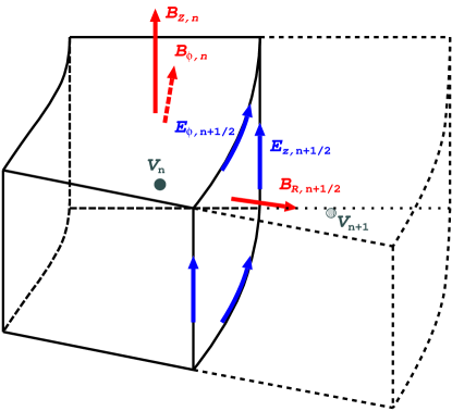
Figure 9: Grid structure at the radial outer boundary, $R=R_{+}$. The outermost active cell labeled with subscript $n$ is drawn by solid lines and the ghost cell with $n+1$ is by dotted lines. Each component of magnetic field is located at the corresponding surface of the cell, and the induced electric field, $\mbox{\boldmath${cE}$}=-\mbox{\boldmath${v\times B}$}$, is at the side. HD variables, represented by $V$, are at the center of the cell.

The constraint transport (CT) method (Evans & Hawley, 1988) is a numerical scheme to update magnetic fields under the constraint of $\mbox{\boldmath${\nabla\cdot B}$}=0$ within the precision of round-off error. In the CT scheme, the three components of the magnetic field are placed on the surfaces of each grid cell (Figure 9). On the other hand, the HD variables are located at the center of the cell. We apply the shearing periodic boundary presented in Subsection 2.2 to these staggered meshes.

C.2.1 Primitive Variables

Let us first explain how we apply the radial shearing boundary condition to the primitive variables, $V=\rho$, ${v}$, ${B}$, and $e$, at ghost cells and at time $t=m$ by eqs.(71) & (72). As for $\rho$, $v_{R}$, and $v_{z}$, we can use the simple scaling relations of eqs. (30) & (31):

$$(\rho R)_{n+1,j_{+g}}=(\rho R)_{1,j_{-a}};\;(\rho R)_{0,j_{-g}}=(\rho R)_{n,j_{+a}},$$ (73)

$$(v_{R})_{n+1,j_{+g}}=(v_{R})_{1,j_{-a}};\;(v_{R})_{0,j_{-g}}=(v_{R})_{n,j_{+a}},$$ (74)

and

$$(v_{z})_{n+1,j_{+g}}=(v_{z})_{1,j_{-a}};\;(v_{z})_{0,j_{-g}}=(v_{z})_{n,j_{+a}}.$$ (75)

We introduced the sum of Maxwell and Reynolds stresses for the angular momentum shearing variable, $S_{{\rm mom},\phi}$ (eq.14) in Subsection 2.2. We utilize $S_{{\rm mom},\phi}$ to determine $v_{\phi}$ and $B_{\phi}$ at the ghost cells. We here assume both HD and magnetic components have the same radial scaling as that of eq. (14), namely

$$\rho v_{R}\delta v_{\phi}\propto\Omega_{\rm eq},$$ (76)

and

$$B_{R}B_{\phi}\propto\Omega_{\rm eq}.$$ (77)

Eqs. (76) & (9) give

$$\Delta\Omega\equiv\frac{\delta v_{\phi}}{R}\propto\Omega_{\rm eq}(R),$$ (78)

and therefore,

$$(\delta v_{\phi}/R\Omega_{\rm eq})_{n+1,j_{+g}}=(\delta v_{\phi}/R\Omega_{\rm eq})_{1,j_{-a}};\;\;(\delta v_{\phi}/R\Omega_{\rm eq})_{0,j_{-g}}=(\delta v_{\phi}/R\Omega_{\rm eq})_{n,j_{+a}}.$$ (79)

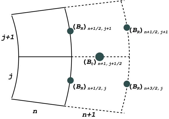
Figure 10: Locations of $B_{R}$ and $B_{\phi}$ (gray dots) near the outer boundary on a horizontal plane. For simplicity, we write $j$ here, though it should be $j_{+g}$ in a strict sense, following eq.(71).

When we apply eq.(77) to the staggered meshes, we need to interpolate because the locations of $B_{R}$ and $B_{\phi}$ are different, as shown in Figure 10. The shearing condition of eq.(77) is applied at the location of $B_{\phi}$ as follows:

$$\left(B_{R}B_{\phi}/\Omega_{\rm eq}\right)_{n+1,(j_{+g})+\nicefrac{{1}}{{2}}}=\left(B_{R}B_{\phi}/\Omega_{\rm eq}\right)_{1,(j_{-a})+\nicefrac{{1}}{{2}}};\;\;\left(B_{R}B_{\phi}/\Omega_{\rm eq}\right)_{0,(j_{-g})+\nicefrac{{1}}{{2}}}=\left(B_{R}B_{\phi}/\Omega_{\rm eq}\right)_{n,(j_{+a})+\nicefrac{{1}}{{2}}}.$$ (80)

We also need an interpolation for $B_{R}$ in eq.(80), because $B_{R}$ is located at different positions from that of $B_{\phi}$ (Figure 10). We take the simple average of the four neighboring locations to calculate $B_{R}$ at $i=1$ & $n$:

$$\left(B_{R}\right)_{1,(j_{-a})+\nicefrac{{1}}{{2}}}=\frac{1}{4}\left[(B_{R})_{\nicefrac{{1}}{{2}},(j_{-a})}+(B_{R})_{\nicefrac{{1}}{{2}},(j_{-a})+1}+(B_{R})_{\nicefrac{{3}}{{2}},(j_{-a})}+(B_{R})_{\nicefrac{{3}}{{2}},(j_{-a})+1}\right]$$

$$\left(B_{R}\right)_{n,(j_{+a})+\nicefrac{{1}}{{2}}}=\frac{1}{4}\left[(B_{R})_{n-\nicefrac{{1}}{{2}},(j_{+a})}+(B_{R})_{n-\nicefrac{{1}}{{2}},(j_{+a})+1}+(B_{R})_{n+\nicefrac{{1}}{{2}},(j_{+a})}+(B_{R})_{n+\nicefrac{{1}}{{2}},(j_{+a})+1}\right].$$ (81)

On the other hand, we have to carefully deal with $B_{R}$ at the ghost cells to avoid numerical cancellation, which causes spurious behavior of $B_{\phi}$. First, we take the simple average of the four neighboring locations in the same manner to eq.(81):

$$\left(B_{R,{\rm av}}\right)_{n+1,(j_{+g})+\nicefrac{{1}}{{2}}}=\frac{1}{4}\left[(B_{R})_{n+\nicefrac{{1}}{{2}},(j_{+g})}+(B_{R})_{n+\nicefrac{{1}}{{2}},(j_{+g})+1}+(B_{R})_{n+\nicefrac{{3}}{{2}},(j_{+g})}+(B_{R})_{n+\nicefrac{{3}}{{2}},(j_{+g})+1}\right]$$

$$\left(B_{R,{\rm av}}\right)_{0,(j_{-g})+\nicefrac{{1}}{{2}}}=\frac{1}{4}\left[(B_{R})_{-\nicefrac{{1}}{{2}},(j_{-g})}+(B_{R})_{-\nicefrac{{1}}{{2}},(j_{-g})+1}+(B_{R})_{\nicefrac{{1}}{{2}},(j_{-g})}+(B_{R})_{\nicefrac{{1}}{{2}},(j_{-g})+1}\right],$$ (82)

where $(B_{R})_{n+\nicefrac{{3}}{{2}},(j_{+g})}$, $(B_{R})_{n+\nicefrac{{3}}{{2}},(j_{+g})+1}$, $(B_{R})_{-\nicefrac{{1}}{{2}},(j_{-g})}$, and $(B_{R})_{-\nicefrac{{1}}{{2}},(j_{-g})+1}$ are still unknown. We here use

$$(B_{R}R)_{n+\nicefrac{{3}}{{2}},(j_{+g})}=(B_{R}R)_{\nicefrac{{3}}{{2}},(j_{-a})};\;(B_{R}R)_{n+\nicefrac{{3}}{{2}},(j_{+g})+1}=(B_{R}R)_{\nicefrac{{3}}{{2}},(j_{-a})+1}$$

$$(B_{R}R)_{-\nicefrac{{1}}{{2}},(j_{-g})}=(B_{R}R)_{n-\nicefrac{{1}}{{2}},(j_{+a})};\;(B_{R}R)_{-\nicefrac{{1}}{{2}},(j_{-g})+1}=(B_{R}R)_{n-\nicefrac{{1}}{{2}},(j_{+a})+1}$$ (83)

which are expected from the radial differential term of $\mbox{\boldmath${\nabla\cdot B}$}=0$. If the signs of $B_{R}$ on the right-hand side of eq.(82) are different, numerical cancellation occasionally occurs to give $(B_{R,{\rm av}})_{n+1,(j_{+g})+\nicefrac{{1}}{{2}}}$ or $(B_{R,{\rm av}})_{0,(j_{-g})+\nicefrac{{1}}{{2}}}$ $\approx 0$, even though all four $B_{R}$ on the right-hand side have finite values. If this is the case, applying $(B_{R})_{n+1,(j_{+g})+\nicefrac{{1}}{{2}}}=(B_{R,{\rm av}})_{n+1,(j_{+g})+\nicefrac{{1}}{{2}}}$ or $(B_{R})_{0,(j_{-g})+\nicefrac{{1}}{{2}}}=(B_{R,{\rm av}})_{0,(j_{-g})+\nicefrac{{1}}{{2}}}$ to eq.(80) would give a spuriously huge absolute value of $(B_{\phi})_{n+1,(j_{+g})+\nicefrac{{1}}{{2}}}$ or $(B_{\phi})_{0,(j_{-g})+\nicefrac{{1}}{{2}}}$.

In order to avoid this unphysical behavior, we set a floor, $B_{R,{\rm min}}$, on the interpolated $B_{R}$:

$$(B_{R})_{n+1,(j_{+g})+\nicefrac{{1}}{{2}}}=\mathrm{sgn}\left[(B_{R,{\rm av}})_{n+1,(j_{+g})+\nicefrac{{1}}{{2}}}\right]\times\max\left[|(B_{R,{\rm av}})_{n+1,(j_{+g})+\nicefrac{{1}}{{2}}}|,(B_{R,{\rm min}})_{n+1,(j_{+g})+\nicefrac{{1}}{{2}}}\right]$$

$$(B_{R})_{0,(j_{-g})+\nicefrac{{1}}{{2}}}=\mathrm{sgn}\left[(B_{R,{\rm av}})_{0,(j_{-g})+\nicefrac{{1}}{{2}}}\right]\times\max\left[|(B_{R,{\rm av}})_{0,(j_{-g})+\nicefrac{{1}}{{2}}}|,(B_{R,{\rm min}})_{0,(j_{-g})+\nicefrac{{1}}{{2}}}\right].$$ (84)

For $B_{R,{\rm min}}$ we take the minimum absolute value of the four neighboring $B_{R}$ multiplied by a factor, $f_{R,{\rm min}}$, of order of unity:

$$(B_{R,{\rm min}})_{n+1,(j_{+g})+\nicefrac{{1}}{{2}}}=f_{R,{\rm min}}\times\min\left(|(B_{R})_{n+\nicefrac{{1}}{{2}},(j_{+g})}|,|(B_{R})_{n+\nicefrac{{1}}{{2}},(j_{+g})+1}|,|(B_{R})_{n+\nicefrac{{3}}{{2}},(j_{+g})}|,|(B_{R})_{n+\nicefrac{{3}}{{2}},(j_{+g})+1}|\right)$$

$$(B_{R,{\rm min}})_{0,(j_{-g})+\nicefrac{{1}}{{2}}}=f_{R,{\rm min}}\times\min\left(|(B_{R})_{-\nicefrac{{1}}{{2}},(j_{-g})}|,|(B_{R})_{-\nicefrac{{1}}{{2}},(j_{-g})+1}|,|(B_{R})_{\nicefrac{{1}}{{2}},(j_{-g})}|,|(B_{R})_{\nicefrac{{1}}{{2}},(j_{-g})+1}|\right)$$ (85)

When $B_{R,{\rm min}}$ is selected in eq.(84) at a ghost cell, the derived $B_{\phi}$ depends on the choice of $f_{R,{\rm min}}$. Accordingly, $f_{R,{\rm min}}$ controls the magnetic pressure across the simulation boundary, $-\partial_{R}(B_{\phi}^{2}/8\pi)$, at the ghost cell. As a result, the accretion velocity, $v_{R}$, also depends on $f_{R,{\rm min}}$. We carefully determine $f_{R,{\rm min}}$ to give the global radial balance of the angular momentum flux between mass accretion the MHD turbulence that was discussed in Sub-subsection 4.2.3. We adopt $f_{R,{\rm min}}=1/\sqrt{2}$ in the simulation we presented in this paper.

We do not directly use shearing variables for $B_{z}$, but take a simple assumption that the initial radial profile is preserved. Then, $B_{z}$ at the ghost cells are determined by

$$(B_{z}R^{q_{B}})_{n+1,j_{+g}}=(B_{z}R^{q_{B}})_{1,j_{-a}};\;\;(B_{z}R^{q_{B}})_{0,j_{-g}}=(B_{z}R^{q_{B}})_{n,j_{+a}}.$$ (86)

In this paper, we adopted $q_{B}=1$, which gives the consistent radial scalings of $v_{R}$ (eq.74), $v_{z}$ (eq.75), $B_{R}$ (eq.83), and $B_{z}$ (eq.86) with $S_{B_{z}}=RcE_{\phi}$ (eq.18).

Although we do not solve an energy equation, for completeness we describe how $e$ is determined at the ghost cells. From $S_{\rm eng}$ (eq.19) and $S_{\rm mass}$ (eq.9), we obtain

$$\left(\frac{v^{2}}{2}+(\gamma-1)e\right)_{n+1,j_{+g}}=\left(\frac{v^{2}}{2}+(\gamma-1)e\right)_{1,j_{-a}};\;\;\left(\frac{v^{2}}{2}+(\gamma-1)e\right)_{0,j_{-g}}=\left(\frac{v^{2}}{2}+(\gamma-1)e\right)_{n,j_{+a}}.$$ (87)

All the three components of ${v}$ are already derived by eqs. (74), (75), & (79), and therefore, from eq.(87) we can determine $e$ at the ghost cells.

C.2.2 Numerical Fluxes

By using the variables, $V^{m}$, at the ghost cells, we can derive the numerical flux, $F^{m+\nicefrac{{1}}{{2}}}=S^{m+\nicefrac{{1}}{{2}}}$, at the simulation boundaries ($i=1/2$ and $n+1/2$) in eq.(69). However, the calculated $S^{m+1/2}$ does not guarantee that eq.(70) will be within the precision of round-off error because of the azimuthal interpolation at the shearing boundary. In order to conserve the invariant quantities introduced in Subsection 2.4 within a round-off error, it is necessary to apply corrections to the derived $S^{m+\nicefrac{{1}}{{2}}}$.

When we apply the shearing periodic condition to the magnetic field, we use $S_{B_{\phi}}=RcE_{\phi}$ (eq.17) and $S_{B_{z}}=cE_{z}$ (eq.18), which are the induced electric fields located at the exact radial boundaries of the simulation box (Figure 9). $E_{\phi}$ and $E_{z}$ at the radial boundaries are related to the conservation of magnetic flux, as we discussed in Subsection 2.4.

In order to conserve the vertical magnetic flux through $z$ planes (eq.28) to round-off error, the line integration of $E_{\phi}$ along the $\phi$ axis at $R_{-}$ and at $R_{+}$ must be equal:

$$\int_{\phi_{-}}^{\phi_{+}}d\phi(RE_{\phi})_{-}=\int_{\phi_{-}}^{\phi_{+}}d\phi(RE_{\phi})_{+},$$ (88)

where subscript ‘$-$’ corresponds to $i=1/2$ and ‘$+$’ to $i=n+1/2$. $E_{\phi}$ at the radial boundaries are evaluated from the boundary cell ($i=1$ or $n$) and the ghost cell ($i=0$ or $n+1$), and they do not usually satisfy the above conservation relation, as previously discussed. We take the average of the original value of $E_{\phi}$ at $R_{\pm}$ and $E_{\phi}$ at $R_{\mp}$ at the corresponding sheared location:

$$(RE_{\phi}^{\rm cr}(\phi))_{-}=\frac{1}{2}\left[(RE_{\phi}(\phi))_{-}+(RE_{\phi}(\phi-\Delta\Omega t))_{+}\right]$$

$$(RE_{\phi}^{\rm cr}(\phi))_{+}=\frac{1}{2}\left[(RE_{\phi}(\phi+\Delta\Omega t))_{-}+(RE_{\phi}(\phi))_{+}\right],$$ (89)

or in the discretized forms,

$$(RE_{\phi}^{\rm cr})_{\nicefrac{{1}}{{2}},j_{-}}=\frac{1}{2}\left[(RE_{\phi})_{\nicefrac{{1}}{{2}},j_{-}}+(RE_{\phi})_{n+\nicefrac{{1}}{{2}},j_{+}}\right]$$

$$(RE_{\phi}^{\rm cr})_{n+\nicefrac{{1}}{{2}},j_{+}}=\frac{1}{2}\left[(RE_{\phi})_{n+\nicefrac{{1}}{{2}},j_{+}}+(RE_{\phi})_{\nicefrac{{1}}{{2}},j_{-}}\right],$$ (90)

The position of $j_{-}$ and $j_{+}$ does not usually match a grid cell, and therefore, the azimuthal interpolation is necessary to derive $(E_{\phi})_{\nicefrac{{1}}{{2}},j_{-}}$ and $(E_{\phi})_{n+\nicefrac{{1}}{{2}},j_{+}}$. We use a simple linear interpolation, which is sufficient to satisfy the conservation relation of eq.(88).

When updating the magnetic fields, we use $E_{\phi}^{\rm cr}(\phi)$, instead of $E_{\phi}(\phi)$, at the $R_{\pm}$ boundaries of $i=1/2$ and $n+1/2$. This correction ensures that the vertical magnetic flux is conserved (eq.28) within the round-off error according to eq.(88).

Similar to the relation between $E_{\phi}$ and $B_{z}$, $E_{z}(=(v_{R}B_{\phi}-v_{\phi}B_{R})/c)$ at the $R_{\pm}$ boundaries regulates the conservation of azimuthal magnetic flux (eq.27). More specifically,

$$\int_{z_{-}}^{z_{+}}dz(E_{z})_{+}=\int_{z_{-}}^{z_{+}}dz(E_{z})_{-}$$ (91)

conserves the azimuthal magnetic flux through shearing planes (eq.27), where the $z$ integral is taken at the radial boundaries of each shearing plane.

We slightly modify the correction method for $E_{\phi}$ (eqs.89 & 90) in order to apply it to $E_{z}$ because $v_{\phi}$ in $E_{z}$ contains the mean rotational velocity that has opposite signs at $R_{+}$ and $R_{-}$. $v_{\phi}B_{R}$ in $E_{z}$ at the two corresponding sheared locations of $R_{-}$ and $R_{+}$ could have very different values. In this case, if we take the local average of the two corresponding sheared locations, as done for $E_{\phi}$ (eq.89), it may cause spurious numerical errors.

Instead of taking the local average, we use the integrated average of $E_{z}$ over the $\phi z$ planes at $R_{\pm}$ to derive a correction,

$$(E_{z}^{\rm cr})_{-}=(E_{z})_{-}+\frac{1}{2}\left[\overline{(E_{z})}_{+}-\overline{(E_{z})}_{-}\right]$$

$$(E_{z}^{\rm cr})_{+}=(E_{z})_{+}+\frac{1}{2}\left[\overline{(E_{z})}_{-}-\overline{(E_{z})}_{+}\right],$$ (92)

where in the discretized form, $(E_{z})_{-}=(E_{z})_{\nicefrac{{1}}{{2}},j_{-}}$ and $(E_{z})_{+}=(E_{z})_{n+\nicefrac{{1}}{{2}},j_{+}}$, and $\overline{(E_{z})}_{\pm}$ is the integrated average,

$$\overline{(E_{z})}_{\pm}=\frac{\int_{\phi_{-}}^{\phi_{+}}d\phi\int_{z_{-}}^{z_{+}}dz(E_{z})_{\pm}}{\int_{\phi_{-}}^{\phi_{+}}d\phi\int_{z_{-}}^{z_{+}}dz}.$$ (93)

By taking the global average, $\overline{(E_{z})}_{\pm}$, random differences between the two $E_{z}$’s at the corresponding sheared locations of $R_{\pm}$ can be canceled out. Therefore, we can reduce spurious errors of the correction when taking the local average by using eq.(92).

One may notice that in eq.(93) only the $z$ integration along both radial boundaries of a shearing plane is sufficient to satisfy the conservation of $\Phi_{\phi}$ from eq.(91). However, the locations of the radial boundaries do not generally match grid cells, and therefore, the $\phi$ interpolation is required to match the time-evolving shearing planes at each time step. It is simpler to take the $\phi$ average without $\phi$ interpolation. Moreover, random errors can further be canceled out by the $\phi$ integration, in addition to the $z$ integration. Therefore, we take both $\phi$ and $z$ integration to derive $\overline{(E_{z})}_{\pm}$.

It is also difficult to check the conservation of $\Phi_{\phi}$ at shearing planes by the same reason explained above. When we numerically test the conservation of $\Phi_{\phi}$, we also check the conservation of $\sum_{\phi}\Phi_{\phi}$.

In our simulations, we implement corrections of the numerical fluxes only in the CT scheme of $E_{\phi}$ and $E_{z}$. If one likes to apply eq.(70) to $S_{\rm mass}$ for mass conservation within the round-off error, the same procedure for $E_{\phi}$ (eqs.89 & 90) can be adopted.

Appendix D Epicyclic Oscillation

We derive eqs.(24) & (25) from the cylindrical shearing box formulation. We neglect the magnetic terms below. The radial component of the momentum flux averaged over the $\phi$ and $z$ directions is

$$\frac{\partial}{\partial t}\langle\rho v_{R}\rangle+\frac{1}{R}\frac{\partial}{\partial R}\langle\rho v_{R}R^{2}\rangle \approx -\frac{\partial\langle p\rangle}{\partial R}+\frac{\langle\rho v_{\phi}^{2}\rangle}{R}-\langle\rho\rangle\frac{GM_{\star}}{R^{2}}+\langle\rho\rangle R\Omega_{\rm eq,0}^{2}+2\Omega_{\rm eq,0}\langle\rho v_{\phi}\rangle$$ (94)

$$= -\frac{\partial\langle\delta p\rangle}{\partial R}+2\left(\Omega_{\rm eq,0}+\frac{v_{\phi,{\rm eq}}}{R}\right)\langle\rho\delta v_{\phi}\rangle+\frac{\langle\rho\delta v_{\phi}^{2}\rangle}{R}$$

$$\approx 2\Omega_{\rm eq,0}\langle\rho\delta v_{\phi}\rangle,$$

where $\delta p=p-p_{\rm eq}$ and we refer to eq.(55) when deriving the second equality. We leave the dominant term of the right-hand side of the second equality to obtain the final expression. The volume integral of eq.(94) gives eq.(24).

The azimuthal component of the $\phi$ and $z$ averaged momentum flux is

$$\frac{\partial}{\partial t}\langle\rho v_{\phi}R\rangle+\frac{1}{R}\frac{\partial}{\partial R}\langle\rho v_{\phi}v_{R}R^{2}\rangle\approx-2\Omega_{\rm eq,0}\langle\rho v_{R}R\rangle.$$ (95)

We take the volume integral of this equation. The second term on the left-hand side is integrated as

$$\int_{R_{-}}^{R_{+}}\frac{1}{R}\frac{\partial}{\partial R}\langle\rho v_{\phi}v_{R}R^{2}\rangle RdR=\langle\rho v_{R}R\rangle\left[Rv_{\phi}\right]_{R{-}}^{R_{+}},$$ (96)

where we factored out the shearing variable of $S_{\rm mass}=\rho v_{R}R$ from the integration. We can expand $R_{\pm}^{2}\approx R_{0}^{2}\left(1+\frac{2(R_{\pm}-R_{0})}{R_{0}}\right)$ and $\Omega_{\rm eq,\pm}\approx\Omega_{\rm eq,0}\left(1\mp\frac{3}{2}\frac{R_{\pm}-R_{0}}{R_{0}}\right)$ for $(R_{+}-R_{-})\ll R_{0}$ and $H_{0}\ll R_{0}$. Then, $\left[Rv_{\phi}\right]_{R{-}}^{R_{+}}$ can be written as

$$(Rv_{\phi})_{+}-(Rv_{\phi})_{-} = R_{+}^{2}(\Omega_{\rm eq,+}-\Omega_{\rm eq,0})-R_{-}^{2}(\Omega_{\rm eq,-}-\Omega_{\rm eq,0})+(R\delta v_{\phi})_{+}-(R\delta v_{\phi})_{-}$$ (97)

$$\approx -\frac{3}{2}R_{0}\Omega_{\rm eq,0}(R_{+}-R_{-})-\frac{1}{2}R_{0}\Omega_{\rm eq,0}\Delta(R_{+}-R_{-})\approx-\Omega_{\rm eq,0}\left(\frac{3}{2}+\frac{\Delta}{2}\right)\int_{R_{-}}^{R_{+}}RdR,$$

where $\Delta\equiv\delta\Omega_{+}/\Omega_{\rm eq,+}=\delta\Omega_{-}/\Omega_{\rm eq,-}$ and we used $R_{0}\approx\frac{1}{2}(R_{-}+R_{+})$ to derive the final expression. Applying eqs.(96) & (97) to the volume integral of eq.(95), we have

$$\frac{\partial}{\partial t}\int_{R_{-}}^{R_{+}}RdR\langle\rho v_{\phi}R\rangle-\Omega_{\rm eq,0}\left(\frac{3}{2}+\frac{\Delta}{2}\right)\int_{R_{-}}^{R_{+}}RdR\langle\rho v_{R}R\rangle=-2\Omega_{\rm eq,0}\int_{R_{-}}^{R_{+}}RdR\langle\rho v_{R}R\rangle,$$ (98)

which is further transformed into

$$\frac{\partial}{\partial t}\left[\rho v_{\phi}R\right]_{V}=-\frac{1}{2}\left(1-\Delta\right)\Omega_{\rm eq,0}\left[\rho v_{R}R\right]_{V}.$$ (99)

We can usually assume $\Delta\ll 1$ and $\frac{\partial}{\partial t}[\rho v_{\phi}R]_{V}=\frac{\partial}{\partial t}[(\rho v_{\phi,{\rm eq}}+\rho\delta v_{\phi})R]_{V}\approx\frac{\partial}{\partial t}[\rho\delta v_{\phi}R]_{V}$, which give eq.(25).

References

- Adachi et al. (1976) Adachi, I., Hayashi, C., & Nakazawa, K. 1976, Progress of Theoretical Physics, 56, 1756
- Armitage (1998) Armitage, P. J. 1998, ApJ, 501, L189
- Bai (2013) Bai, X.-N. 2013, ApJ, 772, 96
- Bai & Stone (2013a) Bai, X.-N., & Stone, J. M. 2013a, ApJ, 767, 30
- Bai & Stone (2013b) —. 2013b, ApJ, 769, 76
- Balbus & Hawley (1991) Balbus, S. A., & Hawley, J. F. 1991, ApJ, 376, 214
- Balbus & Hawley (1998) —. 1998, Reviews of Modern Physics, 70, 1
- Baruteau et al. (2014) Baruteau, C., Crida, A., Paardekooper, S.-J., et al. 2014, Protostars and Planets VI, 667
- Benítez-Llambay & Masset (2016) Benítez-Llambay, P., & Masset, F. S. 2016, ApJS, 223, 11
- Blackman & Nauman (2015) Blackman, E. G., & Nauman, F. 2015, Journal of Plasma Physics, 81, 395810505
- Blandford & Payne (1982) Blandford, R. D., & Payne, D. G. 1982, MNRAS, 199, 883
- Brandenburg et al. (1995) Brandenburg, A., Nordlund, A., Stein, R. F., & Torkelsson, U. 1995, ApJ, 446, 741
- Brandenburg et al. (1996) —. 1996, ApJ, 458, L45
- Carballido et al. (2006) Carballido, A., Fromang, S., & Papaloizou, J. 2006, MNRAS, 373, 1633
- Chandrasekhar (1961) Chandrasekhar, S. 1961, Hydrodynamic and hydromagnetic stability (Oxford: Clarendon)
- Clarke (1996) Clarke, D. A. 1996, ApJ, 457, 291
- Crida & Morbidelli (2007) Crida, A., & Morbidelli, A. 2007, MNRAS, 377, 1324
- Davis et al. (2010) Davis, S. W., Stone, J. M., & Pessah, M. E. 2010, ApJ, 713, 52
- Evans & Hawley (1988) Evans, C. R., & Hawley, J. F. 1988, ApJ, 332, 659
- Ferreira et al. (2006) Ferreira, J., Dougados, C., & Cabrit, S. 2006, A&A, 453, 785
- Flock et al. (2011) Flock, M., Dzyurkevich, N., Klahr, H., Turner, N. J., & Henning, T. 2011, ApJ, 735, 122
- Fromang et al. (2013) Fromang, S., Latter, H., Lesur, G., & Ogilvie, G. I. 2013, A&A, 552, A71
- Fromang & Papaloizou (2007) Fromang, S., & Papaloizou, J. 2007, A&A, 476, 1113
- Gammie (2001) Gammie, C. F. 2001, ApJ, 553, 174
- Gressel et al. (2012) Gressel, O., Nelson, R. P., & Turner, N. J. 2012, MNRAS, 422, 1140
- Guilet & Ogilvie (2012) Guilet, J., & Ogilvie, G. I. 2012, MNRAS, 424, 2097
- Hawley (2000) Hawley, J. F. 2000, ApJ, 528, 462
- Hawley et al. (1995) Hawley, J. F., Gammie, C. F., & Balbus, S. A. 1995, ApJ, 440, 742
- Hayashi (1981) Hayashi, C. 1981, Progress of Theoretical Physics Supplement, 70, 35
- Hirose et al. (2006) Hirose, S., Krolik, J. H., & Stone, J. M. 2006, ApJ, 640, 901
- Hirose & Shi (2019) Hirose, S., & Shi, J.-M. 2019, MNRAS, 485, 266
- Hoshino (2015) Hoshino, M. 2015, Physical Review Letters, 114, 061101
- Io & Suzuki (2014) Io, Y., & Suzuki, T. K. 2014, ApJ, 780, 46
- Jiang et al. (2013) Jiang, Y.-F., Stone, J. M., & Davis, S. W. 2013, ApJ, 778, 65
- Johansen et al. (2006) Johansen, A., Klahr, H., & Henning, T. 2006, ApJ, 636, 1121
- Johansen et al. (2009) Johansen, A., Youdin, A., & Klahr, H. 2009, ApJ, 697, 1269
- Kanagawa et al. (2018) Kanagawa, K. D., Tanaka, H., & Szuszkiewicz, E. 2018, ApJ, 861, 140
- Kimura et al. (2016) Kimura, S. S., Toma, K., Suzuki, T. K., & Inutsuka, S.-i. 2016, ApJ, 822, 88
- Kimura et al. (2019) Kimura, S. S., Tomida, K., & Murase, K. 2019, MNRAS, 485, 163
- Klahr & Bodenheimer (2003) Klahr, H. H., & Bodenheimer, P. 2003, ApJ, 582, 869
- Kobayashi et al. (2016) Kobayashi, H., Tanaka, H., & Okuzumi, S. 2016, ApJ, 817, 105
- Kunz & Lesur (2013) Kunz, M. W., & Lesur, G. 2013, MNRAS, 434, 2295
- Kunz et al. (2016) Kunz, M. W., Stone, J. M., & Quataert, E. 2016, Physical Review Letters, 117, 235101
- Latter et al. (2015) Latter, H. N., Fromang, S., & Faure, J. 2015, MNRAS, 453, 3257
- Lazarian & Vishniac (1999) Lazarian, A., & Vishniac, E. T. 1999, ApJ, 517, 700
- Lesur et al. (2013) Lesur, G., Ferreira, J., & Ogilvie, G. I. 2013, A&A, 550, A61
- Li et al. (2011) Li, Z.-Y., Krasnopolsky, R., & Shang, H. 2011, ApJ, 738, 180
- Lubow et al. (1994) Lubow, S. H., Papaloizou, J. C. B., & Pringle, J. E. 1994, MNRAS, 267, 235
- Lynden-Bell & Pringle (1974) Lynden-Bell, D., & Pringle, J. E. 1974, MNRAS, 168, 603
- Machida et al. (2000) Machida, M., Hayashi, M. R., & Matsumoto, R. 2000, ApJ, 532, L67
- Masada et al. (2012) Masada, Y., Takiwaki, T., Kotake, K., & Sano, T. 2012, ApJ, 759, 110
- Matsumoto & Tajima (1995) Matsumoto, R., & Tajima, T. 1995, ApJ, 445, 767
- McNally & Pessah (2015) McNally, C. P., & Pessah, M. E. 2015, ApJ, 811, 121
- Miller & Stone (2000) Miller, K. A., & Stone, J. M. 2000, ApJ, 534, 398
- Mohandas & Pessah (2017) Mohandas, G., & Pessah, M. E. 2017, ApJ, 838, 48
- Mori et al. (2019) Mori, S., Bai, X.-N., & Okuzumi, S. 2019, arXiv e-prints
- Muto et al. (2010) Muto, T., Suzuki, T. K., & Inutsuka, S.-i. 2010, ApJ, 724, 448
- Nakagawa et al. (1986) Nakagawa, Y., Sekiya, M., & Hayashi, C. 1986, ICARUS, 67, 375
- Nelson & Papaloizou (2004) Nelson, R. P., & Papaloizou, J. C. B. 2004, MNRAS, 350, 849
- Obergaulinger et al. (2009) Obergaulinger, M., Cerdá-Durán, P., Müller, E., & Aloy, M. A. 2009, A&A, 498, 241
- Ogihara et al. (2017) Ogihara, M., Kokubo, E., Suzuki, T. K., Morbidelli, A., & Crida, A. 2017, A&A, 608, A74
- Okuzumi & Hirose (2012) Okuzumi, S., & Hirose, S. 2012, ApJ, 753, L8
- Okuzumi et al. (2014) Okuzumi, S., Takeuchi, T., & Muto, T. 2014, ApJ, 785, 127
- Parkin & Bicknell (2013) Parkin, E. R., & Bicknell, G. V. 2013, ApJ, 763, 99
- Pelletier & Pudritz (1992) Pelletier, G., & Pudritz, R. E. 1992, ApJ, 394, 117
- Penna et al. (2010) Penna, R. F., McKinney, J. C., Narayan, R., et al. 2010, MNRAS, 408, 752
- Pringle (1981) Pringle, J. E. 1981, ARA&A, 19, 137
- Rembiasz et al. (2016) Rembiasz, T., Guilet, J., Obergaulinger, M., et al. 2016, MNRAS, 460, 3316
- Riols et al. (2016) Riols, A., Ogilvie, G. I., Latter, H., & Ross, J. P. 2016, MNRAS, 463, 3096
- Rothstein & Lovelace (2008) Rothstein, D. M., & Lovelace, R. V. E. 2008, ApJ, 677, 1221
- Sano et al. (1999) Sano, T., Inutsuka, S., & Miyama, S. M. 1999, in Astrophysics and Space Science Library, Vol. 240, Numerical Astrophysics, ed. S. M. Miyama, K. Tomisaka, & T. Hanawa (Boston, MA: Kluwer), 383
- Sano et al. (2004) Sano, T., Inutsuka, S.-i., Turner, N. J., & Stone, J. M. 2004, ApJ, 605, 321
- Sano & Stone (2002) Sano, T., & Stone, J. M. 2002, ApJ, 570, 314
- Shakura & Sunyaev (1973) Shakura, N. I., & Sunyaev, R. A. 1973, A&A, 24, 337
- Shi et al. (2010) Shi, J., Krolik, J. H., & Hirose, S. 2010, ApJ, 708, 1716
- Simon et al. (2018) Simon, J. B., Bai, X.-N., Flaherty, K. M., & Hughes, A. M. 2018, ApJ, 865, 10
- Simon et al. (2015) Simon, J. B., Lesur, G., Kunz, M. W., & Armitage, P. J. 2015, MNRAS, 454, 1117
- Stone et al. (1996) Stone, J. M., Hawley, J. F., Gammie, C. F., & Balbus, S. A. 1996, ApJ, 463, 656
- Suriano et al. (2019) Suriano, S. S., Li, Z.-Y., Krasnopolsky, R., Suzuki, T. K., & Shang, H. 2019, MNRAS, 484, 107
- Suzuki & Inutsuka (2009) Suzuki, T. K., & Inutsuka, S.-i. 2009, ApJ, 691, L49
- Suzuki & Inutsuka (2014) —. 2014, ApJ, 784, 121
- Suzuki et al. (2010) Suzuki, T. K., Muto, T., & Inutsuka, S.-i. 2010, ApJ, 718, 1289
- Suzuki et al. (2016) Suzuki, T. K., Ogihara, M., Morbidelli, A., Crida, A., & Guillot, T. 2016, A&A, 596, A74
- Takahashi & Muto (2018) Takahashi, S. Z., & Muto, T. 2018, ApJ, 865, 102
- Takasao et al. (2018) Takasao, S., Tomida, K., Iwasaki, K., & Suzuki, T. K. 2018, ApJ, 857, 4
- Takeuchi & Okuzumi (2014) Takeuchi, T., & Okuzumi, S. 2014, ApJ, 797, 132
- Taki et al. (2016) Taki, T., Fujimoto, M., & Ida, S. 2016, A&A, 591, A86
- Tanaka et al. (2002) Tanaka, H., Takeuchi, T., & Ward, W. R. 2002, ApJ, 565, 1257
- Tanigawa et al. (2012) Tanigawa, T., Ohtsuki, K., & Machida, M. N. 2012, ApJ, 747, 47
- Tomida et al. (2015) Tomida, K., Okuzumi, S., & Machida, M. N. 2015, ApJ, 801, 117
- Turner et al. (2007) Turner, N. J., Sano, T., & Dziourkevitch, N. 2007, ApJ, 659, 729
- Turner et al. (2003) Turner, N. J., Stone, J. M., Krolik, J. H., & Sano, T. 2003, ApJ, 593, 992
- Velikhov (1959) Velikhov, E. P. 1959, Zh. Eksp. Teor. Fiz., 36, 1398
- Yang et al. (2009) Yang, C.-C., Mac Low, M.-M., & Menou, K. 2009, ApJ, 707, 1233
- Zhu et al. (2015) Zhu, Z., Stone, J. M., & Bai, X.-N. 2015, ApJ, 801, 81