Edge states, corner states, and flat bands in a two-dimensional $\cal PT$-symmetric system

Abstract

We study corner states on a flat band in the square lattice. To this end, we introduce a two dimensional model including Su-Schrieffer-Heeger type bond alternation responsible for corner states as well as next-nearest neighbor hoppings yielding flat bands. The key symmetry of the model for corner states is space-time inversion ($\cal PT$) symmetry, which guarantees quantized Berry phases. This implies that edge states as well as corner states would show up if boundaries are introduced to the system. We also argue that an infinitesimal $\cal PT$ symmetry-breaking perturbation could drive flat bands into flat Chern bands.

I Introduction

Topological properties of gapped ground states for bulk systems could be unveiled by edge states if boundaries are introduced to those systems. This is called bulk-edge (boundary) correspondence Hatsugai (1993), which is nowadays one of the fundamental concepts in condensed matter physics. Except for the quantum Hall effect (QHE) states Thouless et al. (1982); Kohmoto (1985), bulk topological invariants in various classes of topological insulators Kane and Mele (2005); Qi et al. (2008); Schnyder et al. (2008) are not necessarily related with the observables such as the Hall conductance. Therefore, experiments on topological insulators are mainly based on the observation of gapless surface states König et al. (2008); Hasan and Kane (2010); Qi and Zhang (2011); Ando (2013).

The conventional bulk-edge correspondence is the relationship between $d$-dimensional bulk gapped ground states and their $d-1$ dimensional surface gapless states. Recently, the bulk-edge correspondence has been extended to higher-order topological insulators (HOTI) Slager et al. (2015); Benalcazar et al. (2017a, b); Liu and Wakabayashi (2017); Schindler et al. (2018) which have $d-D$ dimensional boundary states generically with $D>1$. The HOTI have been studied extensively with a broad interest in, e.g., symmetry properties and classification Langbehn et al. (2017); Song et al. (2017); Khalaf (2018); Fukui and Hatsugai (2018); Trifunovic and Brouwer (2019); Benalcazar et al. (2019); Matsugatani and Watanabe (2018), model construction Ezawa (2018a, b); Călugăru et al. (2019); Ezawa (2018c), a field theoretical point of view Hashimoto et al. (2017), superconducting systems Wang et al. (2018a); Hsu et al. (2018); Ghorashi et al. (2019), interaction effects You et al. (2018), Floquet systems Bomantara et al. (2019); Rodriguez-Vega et al. (2018), etc. Among them, the HOTI on the breathing Kagome lattice Ezawa (2018a) may be quite interesting, since the model shows a flat band as well. Here, flat band systems Lieb (1989); Mielke (1991); Tasaki (1992); Misumi and Aoki (2017); Rhim and Yang (2019) have been attracting continuous interest, not only in magnetism Lieb (1989); Mielke (1991); Tasaki (1992), but also the fractional QHE Sun et al. (2011); Tang et al. (2011); Neupert et al. (2011); Yang et al. (2012), and superconductivity Kobayashi et al. (2016); Tovmasyan et al. (2016), especially in twisted bilayer graphene Cao et al. (2018); Fatemi et al. (2018); Zou et al. (2018); Rademaker and Mellado (2018); Venderbos and Fernandes (2018); Ramires and Lado (2018); Koshino et al. (2018); Peltonen et al. (2018); Po et al. (2018); Guo et al. (2018); Ochi et al. (2018); Lin et al. (2018); Kennes et al. (2018); Choi and Choi (2018); Qiao et al. (2018); Hejazi et al. (2019); Tarnopolsky et al. (2019), etc. Thus, it may be interesting to investigate more generic flat bands with edge and/or corner states to seek the possibilities of wider topological phases of matter. Such systems would offer a promising platform for studying the interplay among magnetism, superconductivity, and topological phenomena.

In this paper, we investigate a model with inversion ($\cal P$) symmetry as well as time-reversal ($\cal T$) symmetry, which is an extension of the two-dimensional Su-Schrieffer-Heeger (SSH) model in Refs. Benalcazar et al. (2017a, b); Liu and Wakabayashi (2017), including next-nearest neighbor (NNN) hoppings Misumi and Aoki (2017). We first argue that topological invariants for a $\cal PT$-symmetric system are quantized Berry phases Yu et al. (2015); Kim et al. (2015); Huang et al. (2016); Zhang et al. (2016); Chan et al. (2016); Pal and Saha (2018); Pal (2018); Li et al. (2018a); Ahn et al. (2018a); Wang et al. (2018b); Ahn et al. (2018b); Wieder and Bernevig (2018); Chiu et al. (2018); Ahn and Yang (2019); Ghatak and Das (2019) (or polarizations) which could be also topological invariants characterizing the HOTI. Moreover, with fine-tuned parameters for the NNN hoppings, the model allows flat bands. Therefore, we can realize systems in which gapped edge states, corner states and flat bands coexist. We show that the model introduced in this paper has edge states and corner states on a flat-band like the breathing Kagome lattice model Ezawa (2018a). The flat bands with corner states thus derived are near the critical point to flat Chern bands in the sense that the band-crossing with a dispersive band and infinitesimal symmetry-breaking perturbations could turn these (trivial) flat bands into flat Chern bands. To show this, we introduce a locally fluctuating magnetic flux breaking both $\cal T$ and $\cal P$ symmetries but preserving $\cal PT$ symmetry. We show that by increasing a small $\cal PT$ symmetry-breaking perturbation, quantized step-like polarizations are changed into winding polarizations. This is achieved by infinitesimal $\cal P$-breaking perturbations with $\cal T$ invariance.

II $PT$ symmetry

We first argue quantized Berry phases for $\cal PT$-symmetric systems Yu et al. (2015); Kim et al. (2015); Huang et al. (2016); Zhang et al. (2016); Li et al. (2018a); Chiu et al. (2018). Let $H({\bm{k}})$ be a Hamiltonian and $\psi({\bm{k}})$ be the $n$-multiplet, $H({\bm{k}})\psi({\bm{k}})=\psi({\bm{k}}){\cal E}({\bm{k}})$. $\cal PT$ symmetry is described by

$$PTH({\bm{k}})(PT)^{-1}=H({\bm{k}}),$$ (1)

where $T=K$ stands for the complex conjugation, and $(PT)^{2}=1$. This symmetry imposes the constraint on the wave function such that $\psi({\bm{k}})=\left[PT\psi({\bm{k}})\right]U({\bm{k}})=P\psi^{*}({\bm{k}})U({\bm{k}})$, where $U({\bm{k}})$ is a certain $n\times n$ unitary matrix. Let $A_{\mu}({\bm{k}})\equiv{\rm tr}\,\psi^{\dagger}({\bm{k}})\partial_{\mu}\psi({\bm{k}})$ be the U(1) Berry connection, where $\partial_{\mu}=\partial_{k_{\mu}}$ is the partial derivative with respect to the momentum $k_{\mu}$. Then, the constraint on the wave function yields the identity,

$$A_{\mu}({\bm{k}})=-A_{\mu}({\bm{k}})+{\rm tr}\,U^{\dagger}({\bm{k}})\partial_{\mu}U({\bm{k}}).$$ (2)

This implies that the Berry connection is a pure gauge, and hence, the polarization defined by

$$p_{x}(k_{y})\equiv\frac{1}{2\pi i}\int_{-\pi}^{\pi}A_{x}({\bm{k}})dk_{x},$$ (3)

is quantized such that

$$p_{x}(k_{y})=\frac{n_{x}(k_{y})}{2}\quad{\rm mod}~{}1,$$ (4)

where $n_{x}(k_{y})\equiv\frac{1}{2\pi i}\int{\rm tr}\,U^{\dagger}({\bm{k}})\partial_{x}U({\bm{k}})dk_{x}$ is the winding number generically dependent on $k_{y}$. Likewise, the polarization $p_{y}(k_{x})$ is quantized as $p_{y}(k_{x})=\frac{n_{y}(k_{x})}{2}$ mod $1$. If the multiplet under consideration is isolated from other bands by finite direct gaps over the whole Brillouin zone, the integers $n_{\mu}$ ($\mu=x,y$) should be constant, and the set of polarizations $(p_{x},p_{y})$ can serve as the topological invariant for $\cal PT$-symmetric systems. It follows from Eq. (2) that for isolated multiplet bands the Berry curvature vanishes and the multiplet has zero first Chern number.

Let us focus our attention next on one specific band among the multiplets. The band degeneracies of $\cal PT$-symmetric systems have codimension 2, implying that the 2D systems have at most Dirac-like point nodes. With such point nodes, the polarizations $(p_{x}(k_{y}),p_{y}(k_{x}))$ of the specific band have jump discontinuities at those nodes. These discontinuities give rise to $\delta$-function like singularities to Berry curvature. As far as $\cal PT$ symmetry is preserved, the charge of monopoles at point nodes is indistinguishable, because $p=1/2=-1/2$ modulo 1. However, infinitesimal $\cal PT$ symmetry breaking perturbations enables us to observe the charge. If the total monopole charge behind the multiplet under consideration is finite, it yields a finite Chern number if $\cal PT$ symmetry is broken. Therefore, flat bands in $\cal PT$-symmetric systems could be converted into flat Chern bands. Interestingly, this can be achieved by $\cal P$-symmetry-breaking (but $\cal T$-symmetry-preserving) perturbations.

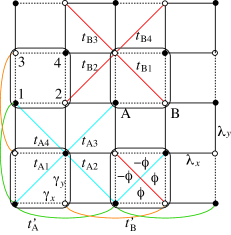
Figure 1: Schematic illustration of the model defined in Eq. (5). $\gamma_{\mu}$ and $\lambda_{\mu}$ ($\mu=x,y$) are nearest neighbor hopping, denoting the SSH-like bond-alternating hoppings, whereas $t_{aj}$ and $t^{\prime}_{a}$ ($a=$A,B and $j=1,\cdots,4$) are next-nearest neighbor hoppings necessary for flat bands. In a lower unit cell, we denote local flux $\phi$ which breaks $\cal T$ and $\cal P$ symmetries but preserves $\cal PT$ symmetry.

III model

We now study the 2D version of the SSH model (Fig. 1) including next-nearest neighbor hoppings, $H({\bm{k}})=H_{\rm SSH}({\bm{k}})+H_{\rm NNN}({\bm{k}})$, where $H_{\rm SSH}$ is the 2D generalization of the SSH model introduced in Benalcazar et al. (2017a, b); Liu and Wakabayashi (2017), and $H_{\rm NNN}$ is the next-nearest neighbor hopping terms necessary for flat bands Misumi and Aoki (2017). They are given by

$$H_{\rm SSH}({\bm{k}})=\begin{pmatrix}0&z_{x}^{*}(k_{x})&z_{y}^{*}(k_{y})&0\\ z_{x}(k_{x})&0&0&z_{y}^{*}(k_{y})\\ z_{y}(k_{y})&0&0&z_{x}^{*}(k_{x})\\ 0&z_{y}(k_{y})&z_{x}(k_{x})&0\end{pmatrix},$$

$$H_{\rm NNN}({\bm{k}})=\begin{pmatrix}d_{\rm A}({\bm{k}})&0&0&z_{\rm A}^{*}({\bm{k}})\\ 0&d_{\rm B}({\bm{k}})&z_{\rm B}^{*}({\bm{k}})&0\\ 0&z_{\rm B}({\bm{k}})&d_{\rm B}({\bm{k}})&0\\ z_{\rm A}({\bm{k}})&0&0&d_{\rm A}({\bm{k}})\end{pmatrix},$$ (5)

where $z_{\mu}(k_{\mu})\equiv\gamma_{\mu}+\lambda_{\mu}e^{ik_{\mu}}$ ($\mu=x,y$), $z_{\rm A}({\bm{k}})=t_{\rm A1}+t_{\rm A2}e^{ik_{x}}+t_{\rm A4}e^{ik_{y}}+t_{\rm A3}e^{i(k_{x}+k_{y})}$, $z_{\rm B}({\bm{k}})=t_{\rm B1}+t_{\rm B2}e^{-ik_{x}}+t_{\rm B4}e^{ik_{y}}+t_{\rm B3}e^{i(-k_{x}+k_{y})}$, and $d_{a}({\bm{k}})=2t_{a}^{\prime}(\cos k_{x}+\cos k_{y})$ ($a=$A,B). For the time being, we assume that all the hopping parameters are real. Then, this model has $\cal T$ symmetry and $\cal P$ symmetry separately, where $\cal P$ symmetry is implemented by $P=\sigma_{1}\otimes\sigma_{1}$. Moreover, when $\gamma_{x}=\gamma_{y}$, $\lambda_{x}=\lambda_{y}$, $t_{{\rm A}j}=t_{{\rm B}j}$ ($j=1,\cdots,4$), and $t^{\prime}_{\rm A}=t^{\prime}_{\rm B}$, $H({\bm{k}})$ has C₄ symmetry. This model interpolates the 2D SSH model Benalcazar et al. (2017b, a); Liu and Wakabayashi (2017) and the flat band model Misumi and Aoki (2017): The latter model is reproduced when $\gamma_{\mu}=\lambda_{\mu}$ for $\mu=x,y$ and $t_{a}^{\prime}=t_{aj}/2$ for $a=$A,B and $j=1,\cdots,4$. For simplicity, we set $\lambda_{x}=\lambda_{y}=\lambda$ and $\gamma_{x}=\gamma_{y}\equiv\gamma$ in this paper. Thus, we assume C₄ symmetry in the basic $H_{\rm SSH}$ part. Then, based on the corner states of exactly solvable $H_{\rm SSH}$, we will investigate the effect of $H_{\rm NNN}$, which is responsible for flat bands.

III.1 Solvable decoupled model

Let us first review the model without $H_{\rm NNN}$ studied in Ref. Liu and Wakabayashi (2017). The SSH part is exactly solvable, since $H_{\rm SSH}({\bm{k}})=h_{\rm SSH}(k_{x})\otimes\mbox{1}\mbox{l}+\mbox{1}\mbox{l}\otimes h_{\rm SSH}(k_{y})$, where $h_{\rm SSH}$ is the conventional 1D SSH model Su et al. (1979). Let $\psi_{n}(k)$ be the eigenstate of $h_{\rm SSH}(k)$ such that $h_{\rm SSH}(k)\psi_{n}(k)=\varepsilon_{n}(k)\psi_{n}(k)$, where $n=\pm$ stands for the positive and negative bands and $\varepsilon_{n}(k)$ ($\varepsilon_{-}(k)=-\varepsilon_{+}(k)$) is the energy eigenvalue. Cleary, the eigenstates and corresponding eigenvalues of $H_{\rm SSH}({\bm{k}})$ are given by $\psi_{nm}({\bm{k}})=\psi_{n}(k_{x})\otimes\psi_{m}(k_{y})$ and $\varepsilon_{nm}({\bm{k}})=\varepsilon_{n}(k_{x})+\varepsilon_{m}(k_{y})$, respectively. It follows that the present 2D model has four bands, one negative $\varepsilon_{--}$, one positive $\varepsilon_{++}$, and doubly-degenerate nearly zero-energy bands $\varepsilon_{+-}$ and $\varepsilon_{-+}$. Each of these four bands has the polarizations $(p_{x},p_{y})=(1/2,1/2)$ for $|\gamma/\lambda|<1$ and $(0,0)$ otherwise. Therefore, at $1/4$- and $3/4$-filling, the polarizations of the ground state are nontrivial when $|\gamma/\lambda|<1$.

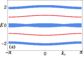
Figure 2: (a) Energy spectrum of the cylindrical system with $\lambda=1$ and $\gamma=0.1$, in which edge states denoted by red lines can be observed. (b) Particle density at $3/4$-filling.

Such a decoupling property also holds for systems with boundaries. For the cylindrical system with an open boundary condition toward the $x$ direction, the wave function of the 2D system is the tensor product of the wave function of the open SSH chain with respect to $x$ and the wave function of the periodic SSH chain with respect to $y$, and the total spectrum is just given by the sum of corresponding energies. Therefore, it is obvious that in the case $|\gamma/\lambda|<1$, the cylindrical system has gapped edge states, as shown in Fig. 2 (a), which are a combination of the Bloch states in the $y$ direction and the edge states in the $x$ direction. These edge states are themselves the 1D SSH states associated with $\psi_{n}(k_{y})$, and their polarization is clearly $p_{y}=1/2$. Therefore, for a full open system with four corners, the model shows corner states exactly at zero energy, even though they are embedded in the bulk spectrum. It thus turns out that the corner states are protected by the nontrivial polarizations $(p_{x},p_{y})$. In addition to the corner states, the model also has edge states, and since the Fermi energy lies within these edge states at $3/4$- ($1/4$-) filling, there appear corner particle (hole) states affected by edge states Benalcazar et al. (2017a, b); Liu and Wakabayashi (2017); Schindler et al. (2018). Figure 2 (b) shows the particle density at $3/4$-filling for the system in Fig. 2 (a) with full open boundary conditions imposed. One can see sharp peaks at four corners as well as the edge state contribution around the boundaries deviated slightly from the average density of the bulk.

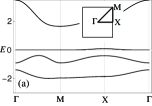
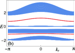
Figure 3: (a) Spectrum of the bulk system. The inset shows the Brillouin zone. (b) Spectrum of the system with open boundary conditions toward the $x$ direction. The edge states are highlighted by red lines. (c) and (d) Particle densities at 3/4- and 1/4-fillings, respectively. The parameters used are $\lambda=1$, $\gamma=0.1$, $t_{\rm A}=0.3$, and $\epsilon_{\rm A}=2$.

III.2 Next-nearest neighbor hopping term and flat band

Let us next include next-nearest neighbor hoppings $H_{\rm NNN}$ to investigate flat bands with corner states. In the case of $\lambda=\gamma$, $t_{{\rm A}j}=t^{\prime}_{\rm A}/2$, and $t_{{\rm B}j}=t^{\prime}_{\rm B}=0$, this model coincides with the model proposed in Misumi and Aoki (2017), implying that the Hamiltonian (5) has a complete flat band separated from a dispersive band by a finite gap. On the other hand, when $\lambda=0$ or $\gamma=0$ as well as $t_{{\rm B}j}=t^{\prime}_{\rm B}=0$, one can prove that the model also has an exact flat band at zero energy for any other parameters $t_{{\rm A}j}$ and $t^{\prime}_{\rm A}$. For simplicity, we restrict our model to

$$t_{{\rm A}j}=2t^{\prime}_{\rm A}=t_{\rm A}\quad(j=1,2,4),\quad t_{{\rm A}3}=\epsilon_{\rm A}t_{\rm A}$$

$$t_{{\rm B}j}=t^{\prime}_{\rm B}=0.$$ (6)

Figure 3 (a) shows the spectrum of the model with small $\gamma=0.1$. The exact flat band when $\gamma=0$ becomes slightly dispersive but is still an almost flat band. All four bands have the nontrivial polarizations $(1/2,1/2)$. Therefore, the system with the open boundary condition toward, e.g., the $x$ direction should have the edge states within the first gap and the third gap guaranteed by $p_{x}=1/2$, as shown in Fig. 3 (b). Moreover, the nontrivial polarization $p_{y}=1/2$ suggests that these edge states would form corner states around zero energy if we further impose the open boundary condition toward the $y$ direction.

Indeed, the spectrum in Fig. 3 (b) can be obtained by an adiabatic deformation of the spectrum in Fig. 2 (c), implying that the edge states in both figures have the same topological property. Namely, those in Fig. 3 (b) have also polarization $p_{y}=1/2$, and they are 1D topological insulators. Thus, for a full open system, corner states should emerge in between those edge states, probably around zero energy. We show in Figs. 3 (c) and (d) the particle density for a system with full open boundary condition at 3/4- and 1/4-filling, respectively. One can observe particle-like and hole-like densities at four corners, which are due to fully occupied and fully unoccupied corner states. A slight effect of the edge states can also be seen, since the Fermi energy is just on the edge states.

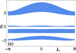
Figure 4: (a) Spectrum of the system with open boundary conditions toward the $x$ direction. (b) Particle density at 3/4-filling. The parameters used are replaced by $\lambda\leftrightarrow\gamma$, $t_{{\rm A}1}\leftrightarrow t_{{\rm A}3}$ in Fig. 3.

These edge and corner states are in sharp contrast to the trivial case, particularly, for the system with replaced parameters $\lambda\leftrightarrow\gamma$ (and also $t_{{\rm A}1}\leftrightarrow t_{{\rm A}3}$) which has the same bulk spectrum by definition. In this system, the polarizations of each band is (0,0), and therefore, there are no edge states for a cylindrical system, as shown in Fig. 4 (a). Correspondingly, the corner states vanish as in Fig. 4 (b) for a full open system.

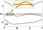
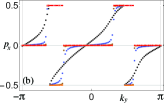
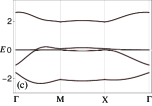
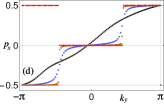
Figure 5: (a) Spectrum with a flat band with a symmetry breaking potential. The red (black) lines show the spectrum with $v_{\rm sb}=0$ ($0.1$). Inset shows the gap formation near the point nodes. The other parameters are $\gamma=0.1e^{i\phi}$ with $\phi=\pi/2$, $t_{{\rm A}}=0.3$, and $\epsilon_{{\rm A}}=2/3$. (b) Polarization $p_{x}(k_{y})$ of the flat (third) band. The red, orange, brown, blue, black dots are the cases with $v_{\rm sb}=0$, $10^{-4}$, $10^{-3}$,$10^{-2}$, $10^{-1}$, respectively. (c) Spectrum and (d) the polarization $p_{x}(k_{y})$ for the same system as (a) and (b) except for the $t^{\prime}_{\rm A}=0$.

III.3 $\cal PT$ symmetry breaking and flat Chern band

So far we have discussed the edge and corner states of the nearly flat band with nontrivial polarizations $(p_{x},p_{y})=(1/2,1/2)$. The quantization of these polarizations is due to $\cal PT$ symmetry, which also ensures vanishing Berry curvatures and Chern numbers. We next consider the possibility of converting such a flat band into a flat Chern band. First, band inversions with dispersive bands may be necessary. For the present model, this can be controlled by the parameter $\epsilon_{\rm A}$ in Eq. (6). Second, ${\cal T}$ symmetry should be broken. To this end, let us introduce locally fluctuating magnetic flux with zero mean Haldane (1988), as denoted in Fig. 1. It can be incorporated simply by replacing $\gamma_{\mu}$ with $\gamma_{\mu}\rightarrow\gamma_{\mu}e^{i\phi}$ for $\mu=x,y$. Such flux $\phi$ breaks not only $\cal T$ symmetry but also $\cal P$ symmetry. Nevertheless, $\cal PT$ symmetry is preserved, implying that the flat band is still a trivial Chern band. In Fig. 5, we show the spectrum (red lines in (a)) and the polarization $p_{x}(k_{y})$ (red dots in (b)) of the flat band for systems with $\cal PT$ symmetry only, including finite local flux $\phi$. The quantized polarization $p_{x}(k_{y})$ of the flat band due to $\cal PT$ symmetry has several jump discontinuities. These are a hallmark of Dirac-like level-crossings, which indeed occur as point nodes because of the codimension 2 of $\cal PT$-symmetric systems. These point nodes give rise to singular Berry curvature. Finally, if $\cal PT$ symmetry-breaking perturbations are introduced, gaps are formed at these point nodes, and discontinuities of the polarization could become smoothly winding between $k_{\mu}=-\pi$ and $\pi$. The winding number of the polarization is merely the Chern number, and thus, a trivial flat band would be converted into a flat Chern band. To show this, we introduce $\cal P$-symmetry breaking potentials to the Hamiltonian

$$H_{\rm on}=v_{\rm sb}\sigma_{3}\otimes\mbox{1}\mbox{l}+v^{\prime}_{\rm sb}\mbox{1}\mbox{l}\otimes\sigma_{3}.$$ (7)

These real onsite potentials of course preserve $\cal T$ symmetry, but they break $\cal PT$ symmetry. Below, we take only the $v_{\rm sb}$ term into account in Eq. (7), setting $v_{\rm sb}^{\prime}=0$, for simplicity. In Fig. 5 (a), we show the spectrum of the system with a small $\cal P$ symmetry breaking potential (black lines). One can observe that small gaps are indeed formed at the point nodes. As can be seen from the polarization $p_{x}(k_{y})$ of the flat band denoted by black points in Fig. 5 (b), the winding number of $p_{x}$ is 2, impling the Chern number $-2$. The direct computation of Chern numbers Fukui et al. (2005) also supports this result. In this figure, one also sees how the step-like function of the polarization for a $\cal PT$ symmetric system changes into a function with a winding number, when one varies the symmetry-breaking potential. Basically, for infinitesimal perturbations, the flat band becomes a flat Chern band. In this sense, the present $\cal PT$ symmetric flat band is just on the critical point from a trivial band to a Chern band. Another example is shown in Fig. 5 (c) and (d) which is the same model as in (a) and (b) except for $t^{\prime}_{\rm A}=0$. The winding number of the polarization implies the Chern number $-1$.

IV Summary and discussions

In summary, we have studied a $\cal PT$ symmetric system having a flat band together with edge and corner states due to nontrivial polarizations. We have argued that the flat band of the model could be changed into a flat Chern band by symmetry-breaking perturbations. For flat band superconductors, the intersection of flat bands and dispersive bands is important Kobayashi et al. (2016); Tovmasyan et al. (2016); Misumi and Aoki (2017). Thus, it may be interesting to consider the possibility of flat band superconductors with edge and/or corner states, especially paying attention to the role played by those states. As argued in Benalcazar et al. (2019), C_n group allows various fractional charges at corners. It may thus be interesting to consider the interplay between flat bands and edge and/or corner states in systems with more generic point group symmetry Benalcazar et al. (2019); Fang et al. (2012). We also note that without C₄ symmetry, $H_{\rm SSH}$ Hamiltonian has unusual corner states inherent to 2D nature of the model Li et al. (2018b). It may be quite interesting to study such a model including $H_{\rm NNN}$.

We would like to thank H. Aoki for fruitful discussions. This work was supported in part by Grants-in-Aid for Scientific Research Numbers 17K05563 and 17H06138 from the Japan Society for the Promotion of Science.

References

- Hatsugai (1993) Y. Hatsugai, Physical Review Letters 71, 3697 (1993).
- Thouless et al. (1982) D. J. Thouless, M. Kohmoto, M. P. Nightingale, and M. den Nijs, Physical Review Letters 49, 405 (1982).
- Kohmoto (1985) M. Kohmoto, Annals of Physics 160, 343 (1985).
- Kane and Mele (2005) C. L. Kane and E. J. Mele, Physical Review Letters 95, 146802 (2005).
- Qi et al. (2008) X.-L. Qi, T. L. Hughes, and S.-C. Zhang, Physical Review B 78, 195424 (2008).
- Schnyder et al. (2008) A. P. Schnyder, S. Ryu, A. Furusaki, and A. W. W. Ludwig, Physical Review B 78, 195125 (2008).
- König et al. (2008) M. König, H. Buhmann, L. W. Molenkamp, T. Hughes, C.-X. Liu, X.-L. Qi, and S.-C. Zhang, J. Phys. Soc. Jpn. 77, 031007 (2008).
- Hasan and Kane (2010) M. Z. Hasan and C. L. Kane, Reviews of Modern Physics 82, 3045 (2010).
- Qi and Zhang (2011) X.-L. Qi and S.-C. Zhang, Reviews of Modern Physics 83, 1057 (2011).
- Ando (2013) Y. Ando, Journal of the Physical Society of Japan 82, 102001 (2013).
- Slager et al. (2015) R.-J. Slager, L. Rademaker, J. Zaanen, and L. Balents, Physical Review B 92, 085126 (2015).
- Benalcazar et al. (2017a) W. A. Benalcazar, B. A. Bernevig, and T. L. Hughes, Physical Review B 96, 245115 (2017a).
- Benalcazar et al. (2017b) W. A. Benalcazar, B. A. Bernevig, and T. L. Hughes, Science 357, 61 (2017b).
- Liu and Wakabayashi (2017) F. Liu and K. Wakabayashi, Physical Review Letters 118, 076803 (2017).
- Schindler et al. (2018) F. Schindler, A. M. Cook, M. G. Vergniory, Z. Wang, S. S. P. Parkin, B. A. Bernevig, and T. Neupert, Science Advances 4, eaat0346 (2018).
- Langbehn et al. (2017) J. Langbehn, Y. Peng, L. Trifunovic, F. von Oppen, and P. W. Brouwer, Physical Review Letters 119, 246401 (2017).
- Song et al. (2017) Z. Song, Z. Fang, and C. Fang, Physical Review Letters 119, 246402 (2017).
- Khalaf (2018) E. Khalaf, Physical Review B 97, 205136 (2018).
- Fukui and Hatsugai (2018) T. Fukui and Y. Hatsugai, Physical Review B 98, 035147 (2018).
- Trifunovic and Brouwer (2019) L. Trifunovic and P. W. Brouwer, Physical Review X 9, 011012 (2019).
- Benalcazar et al. (2019) W. A. Benalcazar, T. Li, and T. L. Hughes, Physical Review B 99, 245151 (2019).
- Matsugatani and Watanabe (2018) A. Matsugatani and H. Watanabe, Physical Review B 98, 205129 (2018).
- Ezawa (2018a) M. Ezawa, Physical Review Letters 120, 026801 (2018a).
- Ezawa (2018b) M. Ezawa, Physical Review B 98, 045125 (2018b).
- Călugăru et al. (2019) D. Călugăru, V. Juričić, and B. Roy, Physical Review B 99, 041301 (2019).
- Ezawa (2018c) M. Ezawa, Physical Review B 98, 201402 (2018c).
- Hashimoto et al. (2017) K. Hashimoto, X. Wu, and T. Kimura, Physical Review B 95, 165443 (2017).
- Wang et al. (2018a) Y. Wang, M. Lin, and T. L. Hughes, Physical Review B 98, 165144 (2018a).
- Hsu et al. (2018) C.-H. Hsu, P. Stano, J. Klinovaja, and D. Loss, Physical Review Letters 121, 196801 (2018).
- Ghorashi et al. (2019) S. A. A. Ghorashi, X. Hu, T. L. Hughes, and E. Rossi, Physical Review B 100, 020509 (2019).
- You et al. (2018) Y. You, T. Devakul, F. J. Burnell, and T. Neupert, Physical Review B 98, 235102 (2018).
- Bomantara et al. (2019) R. W. Bomantara, L. Zhou, J. Pan, and J. Gong, Physical Review B 99, 045441 (2019).
- Rodriguez-Vega et al. (2018) M. Rodriguez-Vega, A. Kumar, and B. Seradjeh (2018), eprint arXiv:1811.04808.
- Lieb (1989) E. H. Lieb, Physical Review Letters 62, 1201 (1989).
- Mielke (1991) A. Mielke, 24, L73 (1991).
- Tasaki (1992) H. Tasaki, Physical Review Letters 69, 1608 (1992).
- Misumi and Aoki (2017) T. Misumi and H. Aoki, Physical Review B 96, 155137 (2017).
- Rhim and Yang (2019) J.-W. Rhim and B.-J. Yang, Physical Review B 99, 045107 (2019).
- Sun et al. (2011) K. Sun, Z. Gu, H. Katsura, and S. Das Sarma, Physical Review Letters 106, 236803 (2011).
- Tang et al. (2011) E. Tang, J.-W. Mei, and X.-G. Wen, Physical Review Letters 106, 236802 (2011).
- Neupert et al. (2011) T. Neupert, L. Santos, C. Chamon, and C. Mudry, Physical Review Letters 106, 236804 (2011).
- Yang et al. (2012) S. Yang, Z.-C. Gu, K. Sun, and S. Das Sarma, Physical Review B 86, 241112 (2012).
- Kobayashi et al. (2016) K. Kobayashi, M. Okumura, S. Yamada, M. Machida, and H. Aoki, Physical Review B 94, 214501 (2016).
- Tovmasyan et al. (2016) M. Tovmasyan, S. Peotta, P. Törmä, and S. D. Huber, Physical Review B 94, 245149 (2016).
- Cao et al. (2018) Y. Cao, V. Fatemi, S. Fang, K. Watanabe, T. Taniguchi, E. Kaxiras, and P. Jarillo-Herrero, Nature 556, 43 EP (2018).
- Fatemi et al. (2018) V. Fatemi, S. Wu, Y. Cao, L. Bretheau, Q. D. Gibson, K. Watanabe, T. Taniguchi, R. J. Cava, and P. Jarillo-Herrero, Science 362, 926 (2018).
- Zou et al. (2018) L. Zou, H. C. Po, A. Vishwanath, and T. Senthil, Physical Review B 98, 085435 (2018).
- Rademaker and Mellado (2018) L. Rademaker and P. Mellado, Physical Review B 98, 235158 (2018).
- Venderbos and Fernandes (2018) J. W. F. Venderbos and R. M. Fernandes, Physical Review B 98, 245103 (2018).
- Ramires and Lado (2018) A. Ramires and J. L. Lado, Physical Review Letters 121, 146801 (2018).
- Koshino et al. (2018) M. Koshino, N. F. Q. Yuan, T. Koretsune, M. Ochi, K. Kuroki, and L. Fu, Physical Review X 8, 031087 (2018).
- Peltonen et al. (2018) T. J. Peltonen, R. Ojajärvi, and T. T. Heikkilä, Physical Review B 98, 220504 (2018).
- Po et al. (2018) H. C. Po, L. Zou, A. Vishwanath, and T. Senthil, Physical Review X 8, 031089 (2018).
- Guo et al. (2018) H. Guo, X. Zhu, S. Feng, and R. T. Scalettar, Physical Review B 97, 235453 (2018).
- Ochi et al. (2018) M. Ochi, M. Koshino, and K. Kuroki, Physical Review B 98, 081102 (2018).
- Lin et al. (2018) X. Lin, D. Liu, and D. Tománek, Physical Review B 98, 195432 (2018).
- Kennes et al. (2018) D. M. Kennes, J. Lischner, and C. Karrasch, Physical Review B 98, 241407 (2018).
- Choi and Choi (2018) Y. W. Choi and H. J. Choi, Physical Review B 98, 241412 (2018).
- Qiao et al. (2018) J.-B. Qiao, L.-J. Yin, and L. He, Physical Review B 98, 235402 (2018).
- Hejazi et al. (2019) K. Hejazi, C. Liu, H. Shapourian, X. Chen, and L. Balents, Physical Review B 99, 035111 (2019).
- Tarnopolsky et al. (2019) G. Tarnopolsky, A. J. Kruchkov, and A. Vishwanath, Physical Review Letters 122, 106405 (2019).
- Yu et al. (2015) R. Yu, H. Weng, Z. Fang, X. Dai, and X. Hu, Physical Review Letters 115, 036807 (2015).
- Kim et al. (2015) Y. Kim, B. J. Wieder, C. L. Kane, and A. M. Rappe, Physical Review Letters 115, 036806 (2015).
- Huang et al. (2016) H. Huang, J. Liu, D. Vanderbilt, and W. Duan, Physical Review B 93, 201114 (2016).
- Zhang et al. (2016) D.-W. Zhang, Y. X. Zhao, R.-B. Liu, Z.-Y. Xue, S.-L. Zhu, and Z. D. Wang, Physical Review A 93, 043617 (2016).
- Chan et al. (2016) Y. H. Chan, C.-K. Chiu, M. Y. Chou, and A. P. Schnyder, Physical Review B 93, 205132 (2016).
- Pal and Saha (2018) B. Pal and K. Saha, Physical Review B 97, 195101 (2018).
- Pal (2018) B. Pal, Physical Review B 98, 245116 (2018).
- Li et al. (2018a) S. Li, Y. Liu, B. Fu, Z.-M. Yu, S. A. Yang, and Y. Yao, Physical Review B 97, 245148 (2018a).
- Ahn et al. (2018a) J. Ahn, D. Kim, Y. Kim, and B.-J. Yang, Physical Review Letters 121, 106403 (2018a).
- Wang et al. (2018b) Z. Wang, B. J. Wieder, J. Li, B. Yan, and B. A. Bernevig (2018b), eprint arXiv:1806.11116.
- Ahn et al. (2018b) J. Ahn, S. Park, and B.-J. Yang (2018b), eprint arXiv:1808.05375.
- Wieder and Bernevig (2018) B. J. Wieder and B. A. Bernevig (2018), eprint arXiv:1810.02373.
- Chiu et al. (2018) C. K. Chiu, Y. H. Chan, and A. P. Schnyder (2018), eprint arXiv:1810.04094.
- Ahn and Yang (2019) J. Ahn and B.-J. Yang, Physical Review B 99, 235125 (2019).
- Ghatak and Das (2019) A. Ghatak and T. Das, Journal of Physics: Condensed Matter 31, 263001 (2019).
- Su et al. (1979) W. P. Su, J. R. Schrieffer, and A. J. Heeger, Physical Review Letters 42, 1698 (1979).
- Haldane (1988) F. D. M. Haldane, Physical Review Letters 61, 2015 (1988).
- Fukui et al. (2005) T. Fukui, Y. Hatsugai, and H. Suzuki, Journal of the Physical Society of Japan 74, 1674 (2005).
- Fang et al. (2012) C. Fang, M. J. Gilbert, and B. A. Bernevig, Physical Review B 86, 115112 (2012).
- Li et al. (2018b) L. Li, M. Umer, and J. Gong, Physical Review B 98, 205422 (2018b).