Identifying Sub-Phenotypes of Acute Kidney Injury using Structured and Unstructured Electronic Health Record Data with Memory Networks

Abstract

Acute Kidney Injury (AKI) is a common clinical syndrome characterized by the rapid loss of kidney excretory function, which aggravates the clinical severity of other diseases in a large number of hospitalized patients. Accurate early prediction of AKI can enable in-time interventions and treatments. However, AKI is highly heterogeneous, thus identification of AKI sub-phenotypes can lead to an improved understanding of the disease pathophysiology and development of more targeted clinical interventions. This study used a memory network-based deep learning approach to discover AKI sub-phenotypes using structured and unstructured electronic health record (EHR) data of patients before AKI diagnosis. We leveraged a real world critical care EHR corpus including 37,486 ICU stays. Our approach identified three distinct sub-phenotypes: sub-phenotype I is with an average age of 63.03$\pm 17.25$ years, and is characterized by mild loss of kidney excretory function (Serum Creatinine (SCr) $1.55\pm 0.34$ mg/dL, estimated Glomerular Filtration Rate Test (eGFR) $107.65\pm 54.98$ mL/min/1.73$m^{2}$). These patients are more likely to develop stage I AKI. Sub-phenotype II is with average age 66.81$\pm 10.43$ years, and was characterized by severe loss of kidney excretory function (SCr $1.96\pm 0.49$ mg/dL, eGFR $82.19\pm 55.92$ mL/min/1.73$m^{2}$). These patients are more likely to develop stage III AKI. Sub-phenotype III is with average age 65.07$\pm 11.32$ years, and was characterized moderate loss of kidney excretory function and thus more likely to develop stage II AKI (SCr $1.69\pm 0.32$ mg/dL, eGFR $93.97\pm 56.53$ mL/min/1.73$m^{2}$). Both SCr and eGFR are significantly different across the three sub-phenotypes with statistical testing plus postdoc analysis, and the conclusion still holds after age adjustment.

1 Introduction

Acute Kidney Injury (AKI) is a critical clinical event characterized by a sudden decrease in kidney function, which affects about 15% of all hospitalizations and more than 50% of patients in intensive care unit (ICU) (Cheng et al., 2017). It is a complex condition, which rarely possesses an unique and obvious pathophysiology (Makris and Spanou, 2016). Patients with AKI usually present a complex etiology, which involves different causes and complicates the clinical manifestations and treatments (Tomašev et al., 2019). For example, sepsis, ischemia, and the nephrotoxicity of drugs frequently co-occur in patients with AKI (Makris and Spanou, 2016; Chertow et al., 2005). Moreover, AKI is a progressive kidney function disorder and has multiple stages in terms of severity, which is associated with a broad spectrum of clinical factors including creatinine, chloride, and hemoglobin measurements, as well as heart and respiration rates. Therefore, identification of AKI subtypes can lead to an improved understanding of the underlying disease etiology and the future development of more targeted interventions and therapies. However, due to the complexity and heterogeneity of AKI, it is challenging to define AKI sub-phenotypes accurately based on clinical knowledge.

In recent years, due to wider availability of electronic health record (EHR) data, researchers have developed data-driven approaches to identify disease sub-phenotypes using EHR data (Fereshtehnejad et al., 2017; Maglanoc et al., 2019). From a data-driven perspective, patient sub-phenotyping is essentially a clustering problem (Zhang et al., 2019; Fereshtehnejad et al., 2017), where patients in the same ”sub-phenotype cluster” tend to be more similar to each other based on disease manifestations derived from their EHRs. Generally speaking, there are three steps for the task of data-driven discovery of sub-phenotypes using EHRs:

• Representation. For each patient in the dataset, we need to first construct an appropriate representation (e.g., vectors (Sun et al., 2012), matrices (Wang et al., 2013), tensors (Luo et al., 2016a) or sequences (Baytas et al., 2017)) of their information derived from the EHRs.

• Clustering. Next, we need to develop or adopt existing clustering algorithms (e.g., hierarchical agglomerative clustering (Fereshtehnejad et al., 2017) or K-means (Zhang et al., 2019)) based on the patient representations derived from previous step to acquire the patient clusters. Each cluster corresponds to an unique sub-phenotype.

• Interpretation. After the patient clusters are obtained, we need to derive a clinical characterization for each of them (usually by identification of features that are discriminative across the different clusters through statistical testing (Fereshtehnejad et al., 2017; Zhang et al., 2019)). This step allows us to appropriately interpret the computationally derived clusters.

Several prior studies have demonstrated the utility of data-driven sub-phenotyping with patient EHRs. For example, Ho et al. (Ho et al., 2014) developed a tensor factorization based phenotyping approach that was capable of exploring the interactions among different modalities in the EHR data (e.g., diagnosis and medication). Zhou et al. (Zhou et al., 2014) proposed a matrix factorization algorithm to first reduce the dimensionality of the event space in the EHRs and then derive the the patient phenotypes in the low-dimensional space. Baytas et al. (Baytas et al., 2017) further developed a deep learning approach to exploit the event temporalities in patient EHR. While promising, these prior efforts were limited to analyzing only structured EHR data. More recent work has also investigated unstructured EHR data to computationally derive sub-phenotypes (Halpern et al., 2016; McCoy Jr et al., 2018). In reality, both structured and unstructured EHR data contain important information about the patients, and therefore, an ideal solution to derive sub-phenotype should integrate all available EHR data. To this end, Pivovarov et al. (Pivovarov et al., 2015) proposed a mixture topic modeling approach for large-scale discovery of computational models of disease or phenotypes. However, their method does not explore the temporality between the clinical events documented in both structured and unstructured EHR data.

In this study, we propose a deep learning model architecture to identify sub-phenotypes of AKI using longitudinal structured and unstructured EHR data. In particular, this study contains two goals. The first goal is to obtain effective representations that can accurately predict the incidence of AKI cases, and the second goal is to identify AKI subtypes on the obtained representations. More concretely, our approach is composed of three steps:

• In the representation step, we choose memory network (MN) (Sukhbaatar et al., 2015) as the backbone of our model, wherein the structured event sequences are inserted into the memory network and the unstructured clinical note series are transformed into a vector through a hierarchical Long Short Term Memory (HieLSTM) model. The vector is then combined with useful information extracted from the memory network to construct a vector representation for each patient. We optimize the model parameters such that the final representation vector can lead to the best prediction performance of a future AKI risk.

• In the clustering step, we first used the student t-distributed Stochastic Neighbor Embedding (t-SNE)(Maaten and Hinton, 2008; Van Der Maaten et al., 2009) to project the patient vectors obtained into a two-dimensional space such that the cluster structure can be inspected visually, and then performed K-means clustering to obtain the patient clusters.

• In the interpretation step, we performed statistical testing and manual evaluation to identify the features that are discriminant across the clusters, and used those features for defining disease sub-phenotypes.

We applied this approach to detect AKI sub-phenotypes using the EHRs from the MIMIC III data set (Johnson et al., 2016), where three distinct sub-phenotypes were identified that align with the different stages of AKI. In the following we introduce our study in detail.

2 Methods

2.1 Data Set, AKI Case Definition, and Patient Features

The EHR data used in this study is from the Medical Information Mart for Intensive Care III (MIMIC-III) database (Johnson et al., 2016), which is a de-identified and publicly available data set. It contains approximately sixty thousand admissions of patients who stayed in critical care units of the Beth Israel Deaconess Medical Center between 2001 and 2012. The patient information contained in this database includes patient demographics, vital signs, laboratory test results, procedures, medications, clinical notes, imaging reports, and patient mortality.

AKI Case Definition: There are four commonly used AKI diagnostic criteria: the Risk-Injury-Failure-Loss-End (RIFLE) criteria (Bellomo et al., 2004), then pediatric RIFLE (pRIFLE) criteria (Akcan-Arikan et al., 2007), the Acute Kidney Injury Network (AKIN) criteria (Pickering and Endre, 2009), and the Kidney Disease: Improving Global Outcomes (KDIGO) criteria (Kellum et al., 2012). KDIGO is the latest and it unified the previous criteria in 2012, which improves the sensitivity of AKI diagnosis and has been widely used by researchers (Makris and Spanou, 2016; Li et al., 2018). In this study, we employ the KDIGO criteria to define AKI cases as follows: (1) Increase in Serum Creatinine (Scr) by $\geq$ 0.3 mg/dl ($\geq$26.5 μmol/l) within 48h; or (2) Increase in SCr to $\geq$1.5 times from the baseline, which is known or presumed to have occurred within the prior 7 days; or (3) Urine volume $<$ 0.5 ml/kg/h for 6h. Moreover, as we will interpret the data-driven sub-phenotypes based on AKI stages, we will consider the following criteria from KDIGO for AKI staging:

Stage 1: SCr is 1.5-1.9 times of baseline, which is known or presumed to have occurred within the prior 7 days; or no less than 0.3 mg/dL (26.5 mol/L) absolute increase in SCr within 48h; or urine volume is less than 0.5 mL/kg/h for 6-12 hours.

Stage 2: SCr is no less than 2.0-2.9 times of baseline, which is known or presumed to have occurred within the prior 7 days; or urine volume is less than 0.5 mL/kg/h for no less than 12 hours.

Stage 3: SCr is no less than 3.0 times from baseline, which is known or presumed to have occurred within the prior 7 days; or increase in SCr is no less than 4.0 mg/dL (353.6 mol/L) within 48h; or initiation of renal replacement therapy; or urine volume is less than 0.3 mL/kg/h for no less than 24 hours; or anuria for no less than 12 hours; or renal replacement therapy required.

Patient Features: We extracted several groups of features from MIMIC-III as follows.

• Demographics: Gender, age and ethnicity.

• Medications: Medications that were administered from the patients’ ICU admission until prediction time. Based on literature analysis and the KDIGO criteria, we mainly consider the following categories: diuretics, Non-steroidal anti-inflammatory drugs (NSAID), radiocontrast agents, and angiotensin.

• Comorbidities: Comorbidities that the patients already have. Based on literature analysis and the KDIGO criteria, we mainly consider the following categories: congestive heart failure, peripheral vascular, hypertension, diabetes, liver disease, myocardial infarction (MI), coronary artery disease (CAD), cirrhosis, and jaundice.

• Chart-events: Vital signs measured at the bedside. Based on literature analysis and the KDIGO criteria, we mainly consider diastolic blood pressure (DiasBP), glucose, heart rate, mean arterial blood pressure (MeanBP), respiration rate, blood oxygen saturation level (SpO2), systolic blood pressure (SysBP), and temperature.

• Lab-events: Laboratory test results performed prior to and during the ICU stay. Based on literature analysis and the KDIGO criteria, we consider the following tests: bicarbonate, blood urea nitrogen (BUN), calcium, chloride, creatinine, hemoglobin, international normalized ratio (INR), platelet, potassium, prothrombin time (PT), partial thromboplastin time (PTT), white blood count (WBC), the average of urine output, and the minimum value of estimated glomerular filtration rate (eGFR) that is computed by MDRD (Modification of Diet in Renal Disease) 4-Variable Equation including age, sex, ethnicity, and serum creatinine (Levey et al., 2006).

2.2 Experimental Setting and Data Pre-Processing

As discussed in the Introduction, the first step of data-driven sub-phenotyping is to learn an appropriate representation for each patient. In our approach, we expect such representation can effectively predict future AKI risk. In particular, because MIMIC-III mainly contains ICU admission data for the patients in critical care, and the same individual might have multiple ICU stays, we define AKI cases and controls based on the records in each ICU stay. More concretely, let $t_{1}$ be the elapsed time (in hours) after the patient was admitted to ICU, from which we will extract the patient records to train our model. Thus $t_{1}$ is also referred to as observation window. The AKI case/control label is defined on the records within $t_{2}$ after $t_{1}$. Thus $t_{2}$ is also referred to as prediction window. In this study, $t_{1}$ is set to 24 hours (or 48 hours) and $t_{2}$ is set to 7 days. The illustration of experimental setting is shown in Figure 1. We choose 7-days as the prediction window according to the definition of AKI by KDIGO criteria. Related study would suggest 7 days as the cut-off for diagnosing AKI (Schneider and Ostermann, 2017). While the 0.3 mg/dl increase for urine is within 48 hours, the definition of stage 1, 2, 3 are 1.5 times of baseline, 2 times of baseline, 3 times of baseline within 7 days, respectively. Technically, when a patient enters the ICU unit they might not have had any kidney injury but the thought is that many of them are at risk due to low blood pressure, inflammation, or sepsis. We exclude patients who were admitted with AKI in the ICU and had AKI in the first 24 hours (or 48 hours) in the ICU. We also exclude patients whose SCr and urine data are missing from the prediction window.

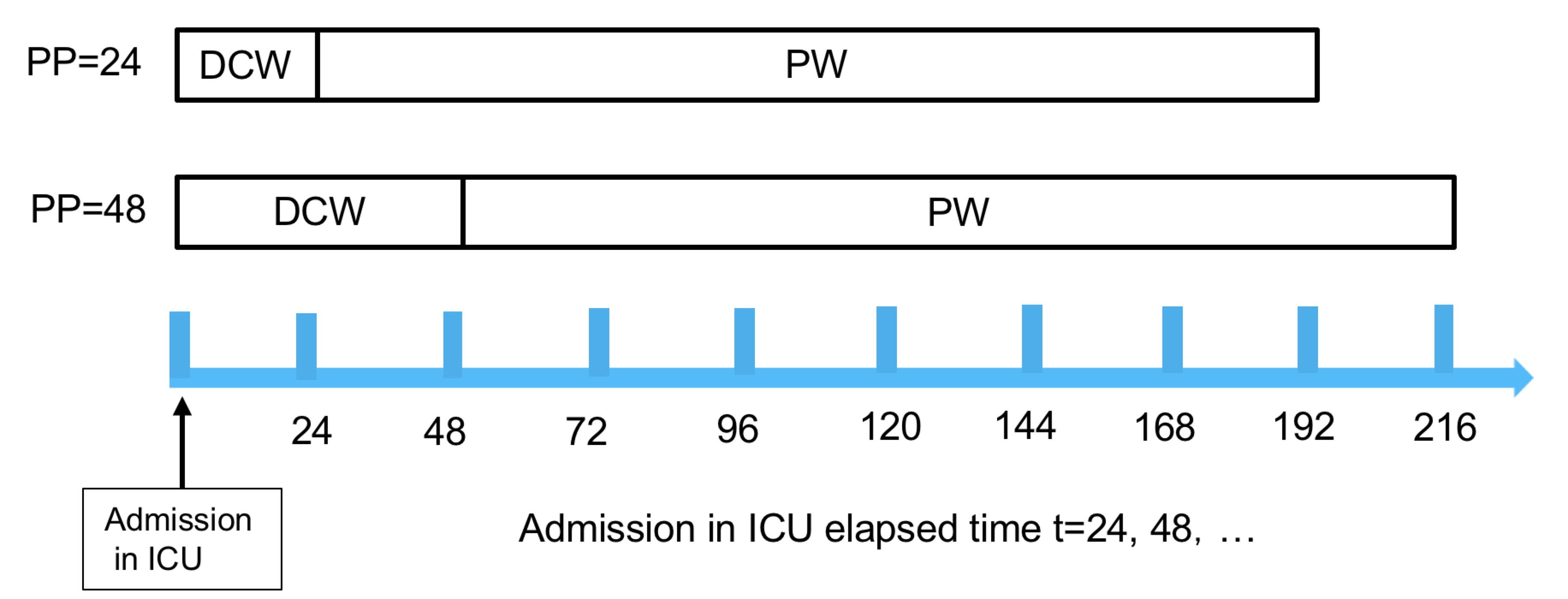
Figure 1: An illustration of AKI prediction in our experimental setting. PP: prediction point; DCW: data collection window; PW: prediction window.

For data pre-processing, we first categorize the observation window into a set of equal-length sub-windows, and we set the sub-window length to 2 hours in our study. The values for each variable are averaged over each sub-window. We impute the missing values by the variable mean and further uniformly scale the values for each variable into the region between 0 and 1. The discrete variables (e.g., medication and comorbidities) are encoded as zero-one multi-hot vectors. For unstructured data, each clinical note is modeled as a sequence of words. The medical term dictionary was constructed based on our prior work (Li et al., 2018), which was further leveraged to filter the clinical notes. In this study, each piece of clinical notes is modeled as a sequence of words, which can keep important medical term words and some corresponding context words. These context words can provide some useful information for modelling each piece of clinical notes when using some deep learning based methods. From these notes, we can obtain some evidence and relationships in terms of the progress of different diseases. Note that, we do not use all words in notes, because the researchers removed some words when building medical term dictionary, e.g., the words with document-frequency under 100 were removed to reduce noise. More details in terms of the process of building medical term dictionary can be referred (Li et al., 2018). Note that each ICU stay typically contains multiple clinical notes. Based on these aforementioned data pre-processing steps, we end up with a total of 37,486 ICU stays including 7,657 AKI cases from 6,933 unique patients, and 29,829 controls from 24,366 unique patients.

2.3 The Proposed Model

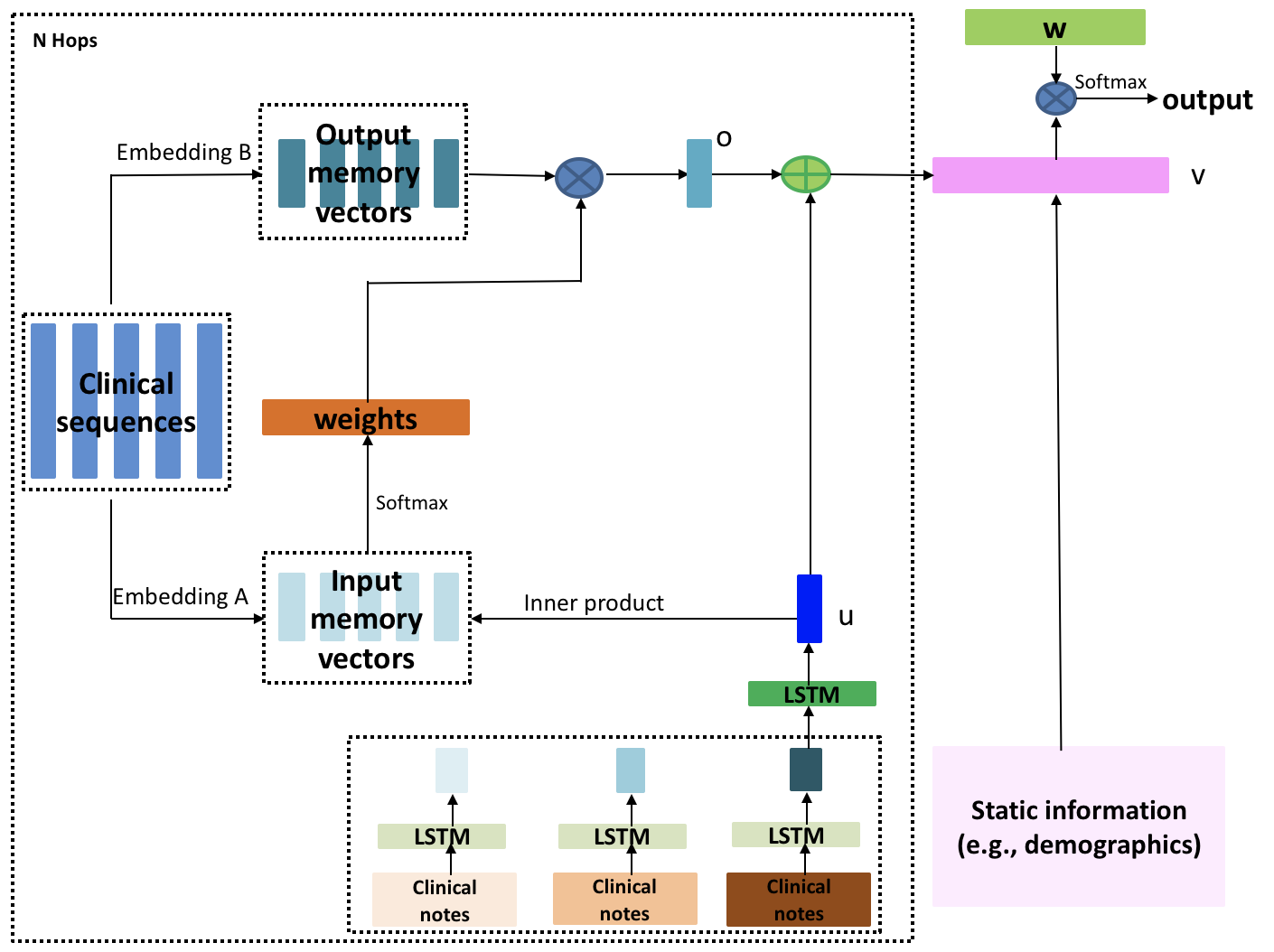
Figure 2: An illustration of the proposed framework. An ICU stay representation $v$ is derived by integrating structured and unstructured EHR data. Time-dependent structured EHR data (clinical sequences) is push into the memory by using embedding matrices $A$ and $B$. Unstructured EHR data (clinical notes) is represented as a vector $u$ by using hierarchical LSTM, which is combined with input memory vectors to retrieve important information from output memory vectors to form a vector $o$. Static information is integrated with $o$ and $u$ to form an ICU stay representative vector $v$.

As stated in the Introduction, there are three key steps in our model. The first step is to construct effective representation vectors. The overall architecture of our model is shown in Figure 2, where we use memory networks (MN) (Weston et al., 2014; Sukhbaatar et al., 2015) as the backbone. The general assumption here is that the AKI risk during a specific ICU stay will be dependent on the information contained in the series of clinical notes (extracted from a hierarchical LSTM model) and structured fields (such as lab tests, vital signs, etc., which are stored in the memory bank) in the EHR before the prediction time point. We further elaborate our model in the following.

MN models have been demonstrated to be very effective in Question-Answering problems (Miller et al., 2016; Bordes et al., 2015). The general setup of an MN model includes a set of inputs $x$ that are to be stored in the memory (which contain information of potential answers), a query $q$, and an answer $a$. The MN model compares an input query $q$ with the information in the memory $x$ and retrieves useful information that is similar to $q$, and then combines the query with the retrieved memory information to predict what would be the right answer. Compared to conventional deep learning models such as Recurrent Neural Network (RNN) (Mikolov et al., 2010), MN models can explicitly control parts of information in the memory that will be extracted, which is much more flexible and interpretable. Multiple previous studies demonstrated that MN based models can obtain better performance than several deep learning models (e.g., LSTM) (Weston et al., 2014; Sukhbaatar et al., 2015). In addition, although several traditional deep learning models (e.g., LSTM) can integrate multi-model data (Rajkomar et al., 2018), the design of $“query”$, $“answer”$, and $“memory”$ in the MN models has a potential to integrate multi-model data to obtain good performance (Zhang et al., 2018).

In our setting, for each ICU stay, our goal is to learn patient representations that can best predict a future AKI risk. We propose to insert the structured EHR information within the observation window into the memory, and transform the series of clinical notes into a query vector. We then compare the query vector with the contents in the memory slots and extract relevant information which are combined with the query to make the AKI prediction. Two major operations in our model are reading and retrieving as discussed below.

Clinical sequences reading: In the MN model, suppose there is an input clinical sequence $s_{j}$, $j=1,...,t$, where $j$ and $t$ are the index of time slots and the number of time slots, respectively. Each item in $s_{j}$ is the value of some clinical variables extracted from the EHR at a certain timestamp. We mainly incorporate time-dependent structured information from charts events variables (e.g., heart rate, respiration rate, systolic blood pressure, and temperature) and lab test results (e.g., calcium, chloride, platelet, creatinine and potassium) into the memory. We employ a fixed number of timestamps $t$ to define the memory size. An embedding matrix $A$ is used to transform input clinical sequences into continuous vectors $z_{j}=As_{j}$, and stored into the memory, which are regarded as a new input memory representation. Meanwhile, we use another embedding matrix $B$ to obtain output memory vectors $e_{j}=Bs_{j}$.

Memory retrieving: The retrieving of memory representation is to find memory vectors from the embedding space. Since different clinical variables in a sequence can contribute differently when it comes to the representation learning for clinical notes, it is necessary to decide which vector to choose. Attentive weights are used here to make a soft combination of all memory vectors. In particular, the weights $\alpha$ are computed by a softmax function on the inner product of the input memory $z_{i}$ and the learned query vector $u$ from the clinical notes:

$$\alpha_{i}=Softmax(u^{T}z_{i})$$ (1)

where $Softmax(r_{i})=e^{r_{i}}/\sum_{j}e^{r_{j}}$. Defined in this way $\alpha$ is a probability vector over the inputs. Once these weights are obtained, we use these weights and output memory vectors $e_{i}$ to obtain a vector $o$ as

$$o=\sum_{i}\alpha_{i}e_{i},$$ (2)

which is combined with $u$ to form a integrated vector $v$ to represent the integrated information within the observation window of an ICU stay.

Generally speaking, such a memory mechanism allows the network to read the input sequences multiple times to update the memory contents at each step and then make a final output. The architecture of multiple layers can be used to collect the information from the memory iteratively and cumulatively for learning the presentations of patients (Rush et al., 2015; Xu et al., 2015). In particular, suppose there are $L$ layer memories for $L$ hop operations, the output feature map at the $l-th$ hop can be rewritten as

$$u^{l+1}=Hu^{l}+o^{l},(l=1,...,L)$$ (3)

where $H$ is a linear mapping and can be beneficial to the iterative updating of $u$. In addition, a layer-wise updating strategy for input and output memory vectors at multiple hops are used, which maintains the same embedding as $A^{1}=...=A^{L}$ and $B^{1}=...=B^{L}$. More details in terms of the process of using multiple layers in memory networks can be referred (Sukhbaatar et al., 2015).

To transform the clinical note series into a vector representation $u$, we use a two-layer hierarchical LSTM (HieLSTM) model. In particular, each ICU stay in the MIMIC dataset comprises multiple clinical notes with timestamps. The bottom layer LSTM is built on each specific clinical note whose word sequence is served as the input. The embedding vector in the hidden layer of the last word is the output. By concatenating the output vectors for all clinical notes in each ICU stay according to their timestamps we obtain the input of the top layer LSTM, and the embedding vector in the hidden layer at the last timestamp will be used as the query.

We compute the probability distribution over the binary class by

$$P=Softmax(w^{T}v)$$ (4)

where $w$ is the coefficient vector and $v$ is the vector combined with memory output $o$ and query $u$. During training, we use cross-entropy to compute the prediction loss

$$\mathcal{L}=\sum_{i}^{N}y_{i}logp_{i}+(1-y_{i})log(1-p_{i})$$ (5)

where $y_{i}$ denotes the label for the $i$-th ICU stay, and $N$ is the total number of ICU stays in training data set.

Our model is implemented with tensorflow 1.7.0 (Abadi et al., 2016) and trained on workstations with NVIDIA TESTA V100 GPUs with mini-batch Adam optimizer (Kingma and Ba, 2014; Zhang et al., 2018).

Based on prior research (Sukhbaatar et al., 2015), we set the memory size and the dimension of embedding as 12 and 128, respectively. For HieLSTM, the dimension of each hidden units in the bottom and top LSTMs are set as 200 and 128, respectively. The final dimension of representation of each ICU stay is 144. In addition, batch size, learning rate, and epoch number are set as 32, 0.01, and 10, respectively.

2.4 Baseline Models

In order to evaluate the effectiveness of the proposed model, we compare its prediction performance with the performances of a set of baseline models. Specifically, we implemented Logistic Regression (LR)(Le Cessie and Van Houwelingen, 1992), Random Forest (RF) (Breiman, 2001), and Gradient Boosting Decision Tree (GBDT) (Friedman, 2002) as the baseline models. To construct the input vector of these models, for time-dependent continuous variables (e.g., lab tests and chart-events) derived from structured EHR data, we calculate the statistics within the observation window including the first, last, average, minimum, maximum, slope and the count. For discrete variables (e.g., medication and comorbidities) derived from structured EHR data, we encode them as zero-one multi-hot vectors. Demographics data are also considered. In particular, gender and ethnicity are seen as discrete variables and age is considered as continuous variable. In this way, the structured EHR data within the observation window of each ICU stay is represented as a 147-dimension feature vector. For unstructured clinical notes, we construct a bag-of-words vector from the collection of clinical notes in each ICU stay. For the implementations of LR and RF, we use the Scikit-learn software library (Pedregosa et al., 2011). For the GBDT, we use the XGBoost software library (Chen and Guestrin, 2016). In addition to these conventional machine learning models, we also implement LSTM and two-layer hierarchical LSTM for prediction based on pure structured and unstructured EHR information.

3 Results and Discussions

3.1 Patient Representation Learning

As introduced above, the first step of our pipeline is to learn an effective representation that can predict the risk of AKI. In experiment, we used the nested cross-validation (Statnikov et al., 2004), which an outer 5-cross-validation was used to split our dataset into training data and testing data, and an inner 5-cross-validation on training data was used for tuning the parameters. Table 1 and Table 2 showed the performance (average $\pm$ standard deviation) of our approach together with the baseline models introduced in Section 2.4 in terms of AUC(Area Under the Receiver Operating Characteristic Curve), precision, and recall (cutoff of 0.5). From these results, we observe that:

• Compared to the performance from only unstructured data (i.e., clinical notes), incorporating both structured and unstructured EHR data can lead to an improved performance. One potential reason is that the structured data contains information related to AKI such as lab tests and chart events.

• The combination of unstructured data and structured data improved the performance, which suggests that there is complementary information contained in both structured and unstructured EHR that is beneficial to the prediction. In particular, clinical notes on MIMIC-III dataset mainly contain several types of notes: (1) echo reports; (2) ECG reports; (3) radiology reports; (4) summary of hospital course of a patient; (5) discharge summary; (6) diagnose descriptions; (7) patient past medical histories. These information can provide multiple evidences and a comprehensive profile for patient current pathophysiologic conditions, for example, patient past medical histories (e.g., cardiac surgery history) can provide implications for patient conditions. The information from multiple kinds of reports may show some connections with AKI.

• Deep learning models (e.g., LSTM and HieLSTM) obtained better results than traditional classification algorithms in all three cases. One potential reason is that such models can capture the temporal dependencies among the structured events and unstructured clinical notes, which could be beneficial to the prediction of AKI risk.

• Our proposed methodology, which integrates both structured and unstructured information through a deep learning model architecture, yields the best performance.

Because the last layer before the output for our proposed model shown in Figure 1 is a simple fully-connected logistic regression, its superior performance really comes from the good patient representation vectors that serve as the inputs to the logistic regressor.

In addition, in order to investigate the importance of using clinical notes, we further examined important words by ranking “feature_importances_” in the GBDT over bag-of-words. The top 10 important words are “lasix”, “ci”, “labile”, “insulin”, “wires”, “cabg”, “dilantin”, “neuro”, “jaundiced”, and “cvp”. These words appear to be clinically meaningful. For example, the word “lasix” is one kind of diuretic, which have a potential to provide treatment for the retention that are caused by kidney dysfunction. The word “cabg (Coronary artery bypass surgery)” provide an implication since these patients have a potential to suffer from kidney injury post-operatively (Kertai et al., 2016).

Table 1: The prediction performance of different methods based on structured and unstructured EHR data produced during 24 hours after admission

Data	Methods	AUC	Precision	Recall
	LR	0.6596$\pm 0.0061$	0.2897$\pm 0.0122$	0.5532$\pm 0.0128$
Unstr	RF	0.6645$\pm 0.0082$	0.2941$\pm 0.013$	0.5536$\pm 0.0135$
	GBDT	0.6797$\pm 0.0071$	0.2978$\pm 0.0135$	0.5603$\pm 0.0142$
	HieLSTM	0.6998$\pm 0.0113$	0.2992$\pm 0.0142$	0.5605$\pm 0.0149$
	LR	0.6823$\pm 0.0052$	0.3115$\pm 0.0142$	0.5834$\pm 0.0152$
Str	RF	0.6999$\pm 0.007$	0.3136$\pm 0.0143$	0.5836$\pm 0.0152$
	GBDT	0.7021$\pm 0.0071$	0.3455$\pm 0.0151$	0.5956$\pm 0.0154$
	LSTM	0.7099$\pm 0.0091$	0.3604$\pm 0.016$	0.5959$\pm 0.0162$
	LR	0.7199$\pm 0.0062$	0.4112$\pm 0.0131$	0.5997$\pm 0.014$
Unstr	RF	0.7201$\pm 0.0094$	0.4222$\pm 0.0132$	0.5998$\pm 0.0143$
+Str	GBDT	0.7319$\pm 0.0083$	0.4336$\pm 0.0142$	0.6009$\pm 0.0145$
	LSTM	0.7431$\pm 0.0095$	0.4531$\pm 0.0149$	0.6101$\pm 0.0152$
	MN+HieLSTM	0.7753$\pm 0.0126$	0.4994$\pm 0.0155$	0.6304$\pm 0.0161$

Table 2: The prediction performance of different methods based on structured and unstructured EHR data produced during 48 hours after admission

Data	Methods	AUC	Precision	Recall
	LR	0.6603$\pm 0.0059$	0.2901$\pm 0.0117$	0.5568$\pm 0.0119$
Unstr	RF	0.6651$\pm 0.0074$	0.2952$\pm 0.014$	0.5598$\pm 0.0136$
	GBDT	0.6802$\pm 0.007$	0.2983$\pm 0.0141$	0.5692$\pm 0.0149$
	HieLSTM	0.7002$\pm 0.0116$	0.3001$\pm 0.0144$	0.5703$\pm 0.0151$
	LR	0.6899$\pm 0.0047$	0.3126$\pm 0.0142$	0.5935$\pm 0.0153$
Str	RF	0.7003$\pm 0.006$	0.3145$\pm 0.0145$	0.5991$\pm 0.0152$
	GBDT	0.7091$\pm 0.0069$	0.3502$\pm 0.0151$	0.5999$\pm 0.0155$
	LSTM	0.7133$\pm 0.0088$	0.3664$\pm 0.0163$	0.6002$\pm 0.0163$
	LR	0.7211$\pm 0.0058$	0.4201$\pm 0.0142$	0.6089$\pm 0.0148$
Unstr	RF	0.7293$\pm 0.0095$	0.4289$\pm 0.0135$	0.6112$\pm 0.0149$
+Str	GBDT	0.7345$\pm 0.0084$	0.4397$\pm 0.0141$	0.6119$\pm 0.0152$
	LSTM	0.7505$\pm 0.0093$	0.4609$\pm 0.0152$	0.6198$\pm 0.0159$
	MN+HieLSTM	0.7798$\pm 0.0131$	0.5011$\pm 0.0162$	0.6397$\pm 0.0177$

3.2 Identifying AKI Sub-Phenotypes

We take EHR data produced during 24 hours after admission (i.e., pp =24 in Figure 1) as an example to investigate the discovering of AKI sub-phenotypes and perform statistical analysis in the following experiments. In particular, after the patient representations were obtained, we first used student t-distributed Stochastic Neighbor Embedding (t-SNE) (Maaten and Hinton, 2008; Van Der Maaten et al., 2009) to embed the patient data into a 2-dimensional space, such that the information can be visually inspected for identification of potential clusters. Then K-means clustering was performed in the 2-dimensional space to computationally identify the clusters. In our study, since the goal is to identify AKI sub-phenotypes, we perform clustering on the representation vectors of all the 7,657 AKI cases.

The results of t-SNE embedding and clustering results are shown in Figure 3 and Figure 4. We consider PCA and auto-encoder methods as two baselines to compare the clustering results. Compared with Figure 3 (a)(b) and Figure 4 (a)(b), the three sub-phenotype depicted in Figure 3 (c) and Figure 4 (c) are much more salient, with a better separation in scatterplot (smaller intra-cluster distance and larger inter-cluster distance). The optimal number of clusters, which is three in this case, is determined by the Mcclain-Rao index (McClain and Rao, 1975). The identified patient clusters are represented with different colors in Figure 4. In the following subsection, we discuss the interpretation of these computationally derived AKI sub-phenotypes.

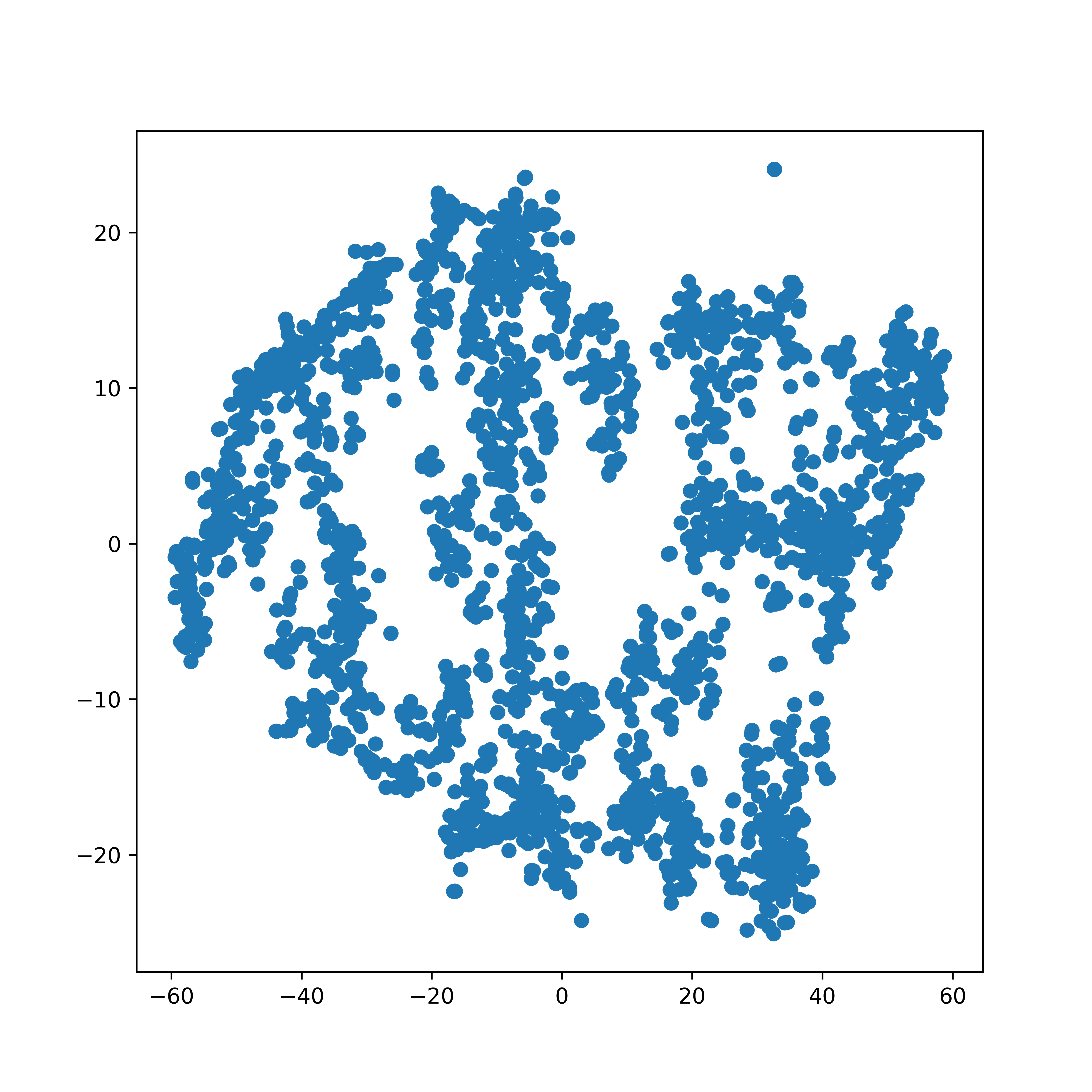
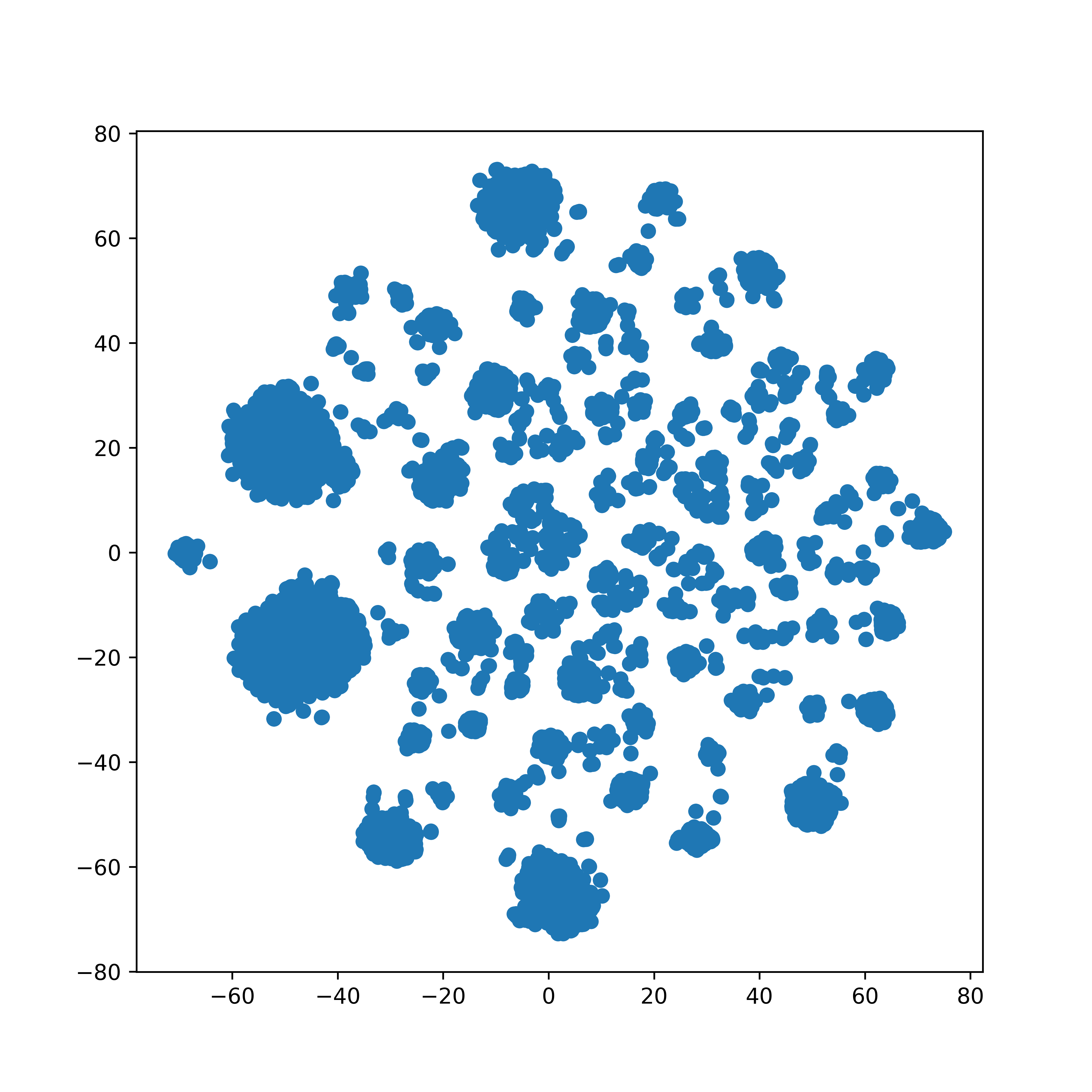
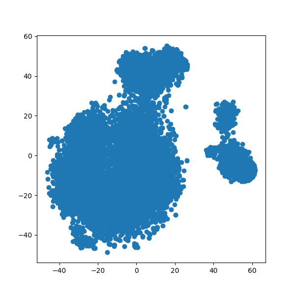
Figure 3: The result of t-SNE: (a), (b), and (c) indicate the representation of patients is obtained by PCA, auto-encoder, and our method, respectively.

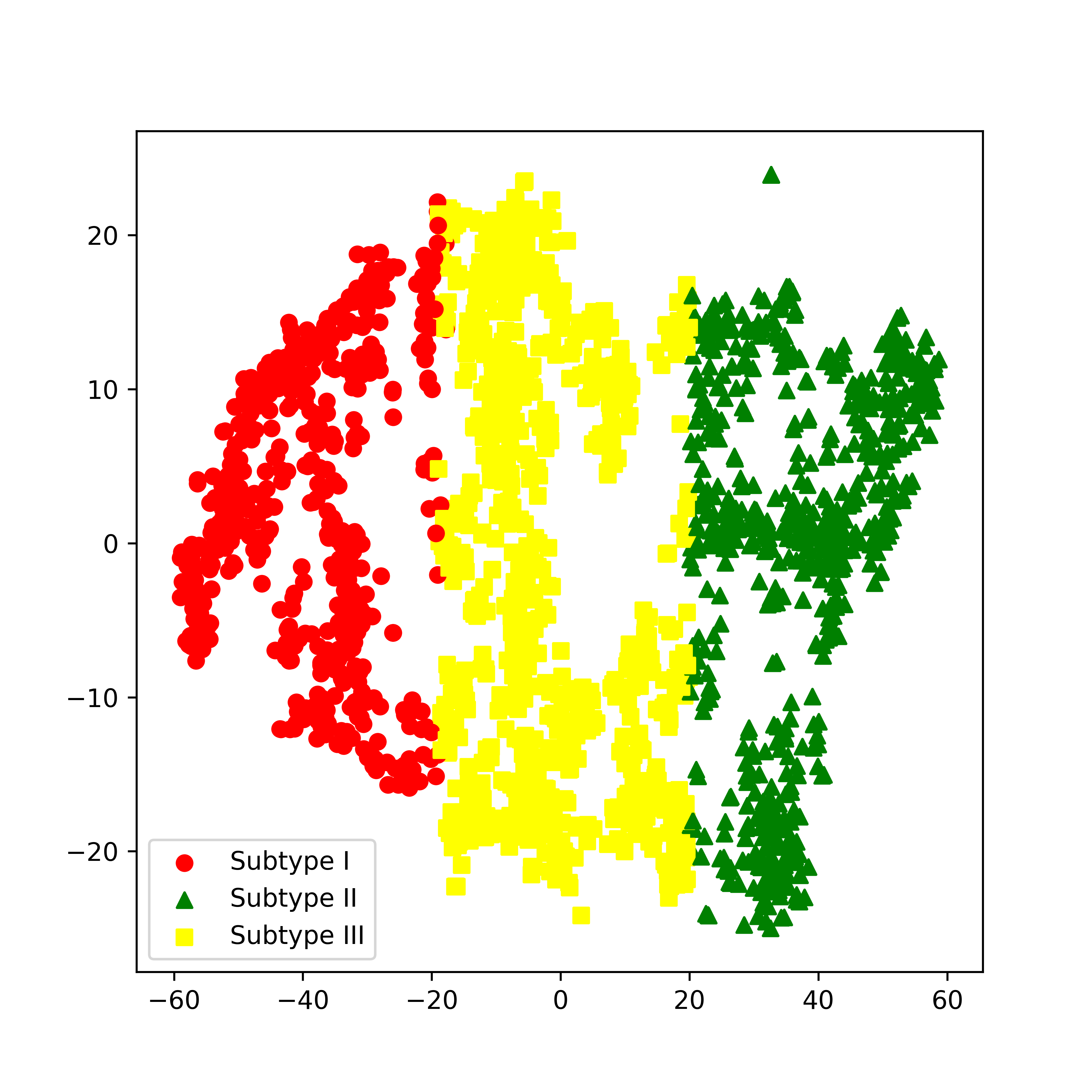
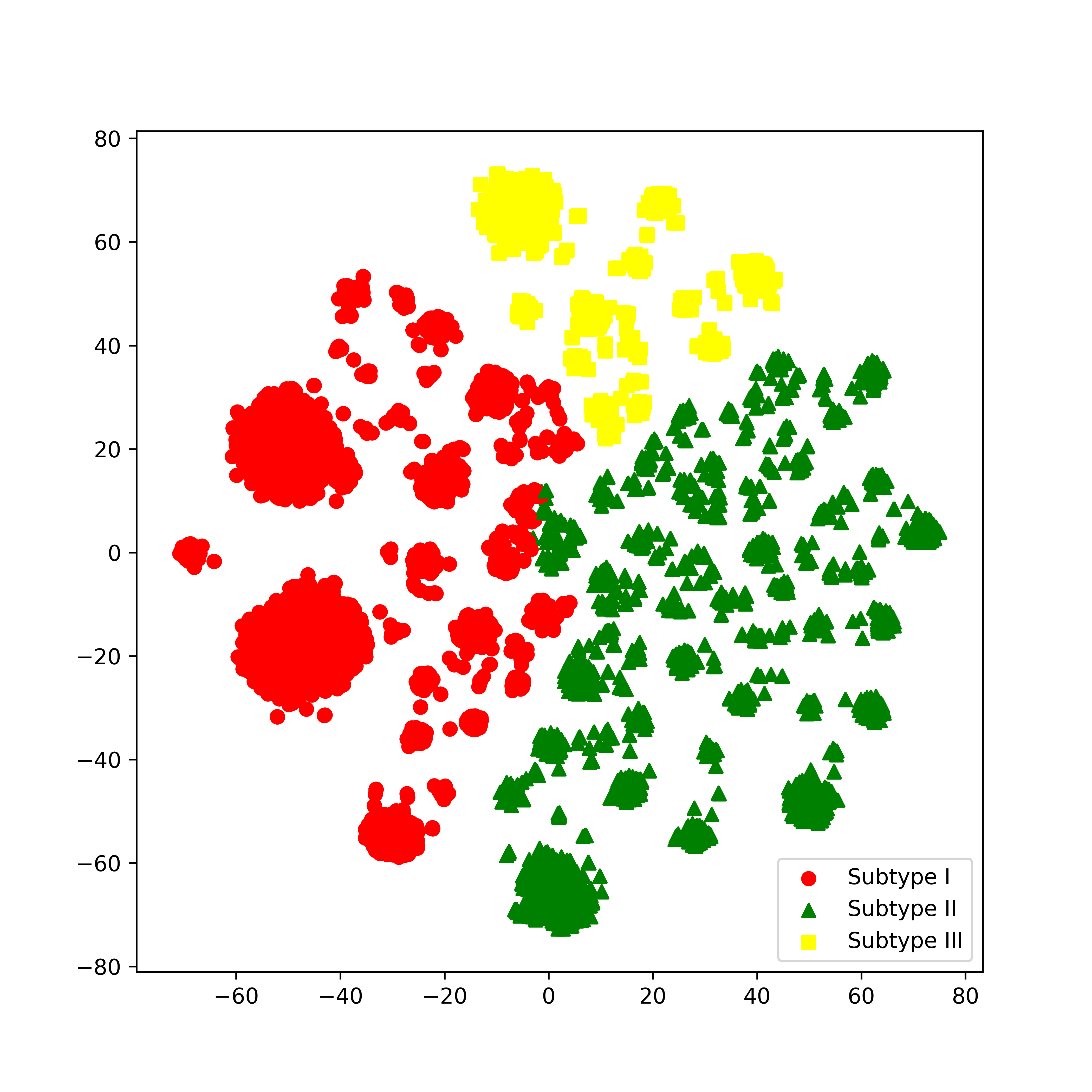
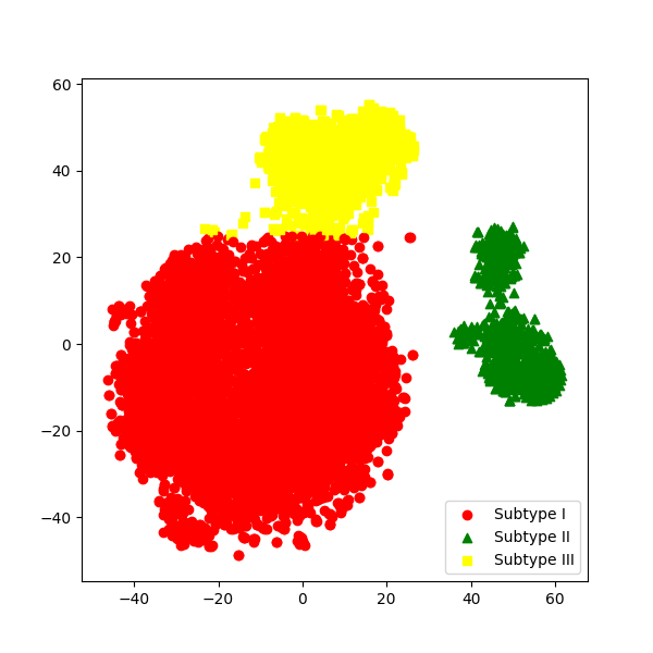
Figure 4: The results of k-means clustering: (a), (b), and (c) indicate the representation of patients is obtained by PCA, auto-encoder, and our method, respectively.

3.3 AKI Sub-Phenotype Interpretation

In order to interpret the three sub-phenotypes, we performed statistical analyses on each of them to identify the patient features that are discriminative among them. In particular, we performed Chi-square test (Lowry, 2014) and One-way ANOVA test (McDonald, 2009) for normally distributed features, and non-parametric testing (Kruskal and Wallis, 1952) for features that are not normally distributed. Posthoc Tukey HSD test (Tukey et al., 1949) was performed for multiplicity correction. Note that, the average of multiple measurements in terms of continuous variables within first 24-hour of admission are computed for statistical comparison between sub-phenotypes. The results are shown in Table 3 and Table 4. From these tables, we can see that the following features are significantly different across the three subtypes: Glucose, Albumin, Diastolic Blood Pressure (DiasBP), Age, Lactate, Creatinine, Hemoglobin, Partial Thromboplastin Time (PTT), White Blood Count (WBC), Urine, and estimated Glomerular Filtration Rate (eGFR). After Age adjustment, the following features are still significantly different:

• Glucose. Diabetes has been shown to be a big risk factor for kidney disease and there are lots of studies on diabetic kidney disease (de Boer et al., 2011; Seaquist et al., 1989; Tuttle et al., 2014). It has also been shown that “AKI risk is most likely being increased in diabetic individuals” (Patschan and Müller, 2016).

• Albumin. Albumin is a protein made by the liver. When the kidney begins to fail, the albumin will leak to the urine and cause a low blood albumin.

• Creatinine. Creatinine is a waste product from the normal breakdown of muscle tissue, which is filtered through the kidneys and excreted in urine. Creatinine level measures the kidney function.

• WBC. The white blood cells are cells fighting infections. A high WBC level may indicate problems like infection or inflammation. As inflammatory response plays a key role in the development of AKI, there are also studies on how WBC and AKI are related (e.g., (Han et al., 2014)).

• Urine. This is the 24-hour urine volume test, which measures the kidney function.

• eGFR. This stands for the glomerular filtration rate estimated based on the creatinine test. It also measures the kidney function.

Therefore, all these identified feature variables are highly correlated with kidney function and AKI.

We further demonstrate the values of these features in different sub-phenotypes in Figure 5. From the figure we can see that sub-phenotype I is with mild kidney dysfunction and sub-phenotype II is with severe kidney dysfunction, while sub-phenotype III is in between.

Table 3: The results of statistical analyses on discrete variables (Number(Percentage), ^aChi-square test)

	Subtype I	Subtype II	Subtype III	Unadjusted	Adjusted
	(N=4553)	(N=672)	(N=2432)	P-value	ANCOVA∗
Male	2928(64.31%)	310(46.13%)	1334(54.85%)	0.520a	0.512
Female	1625(35.69%)	362(53.87%)	1098(45.15%)
Ethnicity_White	924(20.29%)	94(13.99%)	603(24.79%)
Ethnicity_Black	2514(55.22%)	463(68.9%)	1315(54.07%)	0.567a	0.602
Ethnicity_Asian	674(14.8%)	72(10.71%)	408(16.78%)
Ethnicity_others	441(9.69%)	43(6.4%)	106(4.39%)
Diuretics	601(13.2%)	171(25.44%)	406(16.69%)	0.542a	0.432
Nsaid	555(12.19%)	167(24.85%)	399(16.41%)	0.482a	0.543
Angiotensin	641(14.08%)	174(25.89%)	418(17.19%)	0.540a	0.603
CHF	2739(60.16%)	441(65.63%)	1532(62.99%)	0.534a	0.624
PV:	677(14.87%)	115(17.11%)	455(18.71%)	0.591a	0.577
Hypertension	2759(60.6%)	405(60.27%)	1433(58.92%)	0.589a	0.612
Diabetes	1409(30.95%)	298(44.35%)	1081(44.45%)	0.457a	0.521
LD	602(13.22%)	103(15.33%)	341(14.02%)	0.591a	0.614
Mi	567(12.45%)	99(14.73%)	364(14.97%)	0.063a	0.145
Cad	1632(35.84%)	321(47.76%)	1210(49.75%)	0.465a	0.513
Cirrhosis	410(9.01%)	81(12.05%)	291(11.97%)	0.563a	0.633
Jaundice	201(4.41%)	46(6.85%)	149(6.13%)	0.313a	0.453

^∗ANCOVA was performed to adjust significant in terms of age variable. CHF: Congestive Heart Failure; PV: Peripheral Vascular; LD: Liver Disease; CAD: Coronary Artery Disease; MI: Myocardial Infarction.

Table 4: The results of statistical analyses on continuous variables (Mean (Standard Deviation), ^bOne-way ANOVA test, ^cKruskal-Wallis H-test)

	Subtype I	Subtype II	Subtype III	Unadjusted	Adjusted
	(N=4553)	(N=672)	(N=2432)	P-value	ANCOVA ∗ P-value
Glucose	134.32(40.66)	145.56(46.67)	144.22(46.67)	$<$0.001b (I vs II, III)	$<$0.001
Albumin	3.99(0.52)	3.01(0.64)	3.51(0.51)	$<$0.001c (I vs II, III, II vs III)	$<$0.001
AST	82.28(15.00)	85.54(20.83)	83.59(19.13)	0.561b	0.665
Bilirubin	1.41(2.91)	4.87(5.61)	4.68(4.97)	0.538c	0.672
DiasBP	58.64(12.24)	61.13(12.53)	60.45(12.62)	0.004b (I vs II, III)	0.165
Age	63.03(17.25)	66.81(10.43)	65.07(11.32)	$<$0.001b (I vs II, III)	- - -
Lactate	2.16(1.05)	4.91(1.58)	2.97(1.38)	0.012c (I vs II, III, II vs III)	0.025
pH	7.38(0.06)	7.37(0.07)	7.36(0.08)	0.416c	0.565
HeartRate	87.22 (17.09)	90.65(16.26)	86.12(15.09)	0.564b	0.597
MeanBP	76.09(13.25)	78.46(13.67)	79.02(11.40)	0.500b	0.776
RespRate	18.08(4.44)	20.26(4.75)	19.19(4.01)	0.403b	0.465
SpO2	96.37(1.97)	96.27(2.16)	97.23(2.13)	0.481c	0.374
SysBP	115.67(15.94)	120.22(18.11)	120.43(17.63)	0.432c	0.254
Temp	36.85(0.62)	36.82 (0.66)	36.82(0.62)	0.231b	0.432
Bicarbonate	23.87(4.16)	24.70(4.83)	24.51(4.60)	0.542c	0.654
BUN	28.66(22.74)	28.65(24.77)	27.66(21.34)	0.501c	0.776
Calcium	8.36(0.73)	8.40(0.74)	8.78(0.70)	0.378b	0.443
Chloride	105.19(5.45)	102.22(5.90)	103.38(5.62)	0.3423b	0.665
Creatinine	1.55(0.34)	1.96(0.49)	1.69(0.32)	$<$0.001c (I vs II, III, II vs III)	$<$0.001
Hemoglobin	13.55(1.76)	17.18(1.55)	15.53(1.91)	$<$0.001b(I vs II, III, II vs III)	0.101
INR	1.47(0.72)	1.54(1.04)	1.47(0.94)	0.334c	0.554
Platelet	242.08(43.63)	384.96(115.46)	265.31(44.64)	0.521b	0.654
Potassium	4.24(0.56)	4.25(0.56)	4.22(0.54)	0.443c	0.556
PT	15.45(5.76)	17.30(7.45)	15.55(6.38)	0.346c	0.564
PTT	35.12(18.55)	39.24(14.42)	36.94(17.18)	$<$0.001c (II vs III, I)	0.201
WBC	10.59(8.72)	15.71(7.97)	13.23(5.14)	$<$0.001c (I vs II, III, II vs III)	$<$0.001
Urine	1.35(0.24)	1.02(0.25)	1.19(0.25)	$<$0.001c (I vs II, III, II vs III)	$<$0.001
eGFR	107.65(54.98)	82.19(55.92)	93.97(56.53)	$<$0.001c (I vs II, III, II vs III)	$<$0.001

^∗ANCOVA was performed to adjust significant in terms of age variable. AST: Aspartate Aminotransferase in blood; DiasBP: Diastolic Blood Pressure; MeanBP: Mean arterial Blood Pressure; RespRate: Respiration Rate; SysBP: Systolic Blood Pressure; Temp: Temperature; BUN: Blood Urea Nitrogen; INR: International Normalized Ratio; PT: Prothrombin Time; PTT: Partial Thromboplastin Time; WBC: White Blood Count; eGFR: estimated Glomerular Filtration Rate.

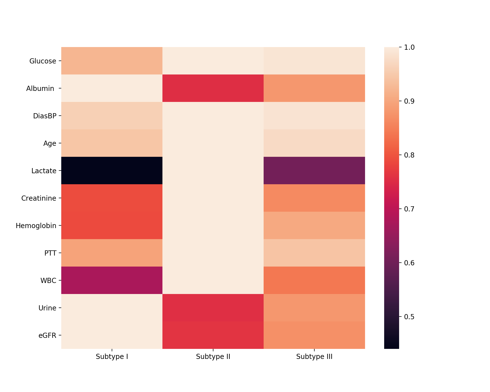
Figure 5: The illustration of heatmap in terms of significant continuous variables in each subtypes.

In order to further validate our observations, we checked the AKI severity of those patients in different sub-phenotypes. We used the AKI staging criteria from KDIGO as we introduced in Section 2.1. We found that sub-phenotype I is mainly with stage I, sub-phenotype II is mainly associated with stage III AKI, while sub-phenotype III is mainly associated with stage II AKI. The compositions of the three sub-phenotypes with respect to the AKI stages are summarized in Table 5.

Table 5: The statistical results for AKI stages and subtypes

	Stage_1	Stage_2	Stage_3
Subtype I (N=4553)	3236(71.07%)	957(21.02%)	360(7.9%)
Subtype II (N=672)	75(11.16%)	171(25.45%)	426(63.39%)
Subtype III (N=2432)	386(15.87%)	1609(66.16%)	437(17.97%)

4 Conclusions and Future Directions

In this paper we propose a data-driven approach for identification of AKI sub-phenotypes. Our approach is composed of three steps. In the first step we develop a memory network based architecture to predict the AKI risk by integrating both the structured and unstructured information in patient EHRs. In the second step we will perform clustering based on the patient representations derived from the first step. In the third step we identify important features that are significantly different across the different clusters and use them to interpret the clusters. On the MIMIC III data set, we identified three AKI sub-phenotypes, and they correlate well with the three stages of AKI very well.

There are two main points in terms of the clinical significance of this study. In particular, firstly, the experimental setting on the proposed model is based on prediction for a patient whether or not suffering from AKI in the next 7 days. The experimental results show that the proposed model has the potential to obtain a better representation. One of the clinical implications of this study is that, for a new patient admitted in ICU, the proposed model can make a prediction with high accuracy for the patient whether or not suffering from AKI. Secondly, since the etiology of AKI is complex, it might be not enough to discover all the subtypes using known rules and some important factors. The proposed model used all raw data to obtain patient representations and discover subtypes, which has the potential to provide some important information assisting clinicians to understand the patient conditions (e.g., the severity of AKI in the next 7 days) in time and take appropriate actions.

For the interpretation step, multiple-testing adjustment was applied to the p-value in our reported results. Note that, the clusters were trained using structured and unstructured data. The variables in reported statistical results are from structured data, which is a part of data used for training clusters. The p-values of these variables may be not very rigorous hypothesis testing.

In the future, our proposed approach can be improved from the following aspects (1) The proposed method is completely data-driven. We can consider how to combine AKI domain knowledge in the model building process. (2) We can add components such as attention mechanism to enhance the model interpretability. (3) We will consider more important variable categories (e.g., interventions, transfusions, diagnostics)(Koyner et al., 2018; Tomašev et al., 2019) and replicate the identified sub-phenotypes on more data sets.

References

References

- Cheng et al. (2017) Peng Cheng, Lemuel R Waitman, Yong Hu, and Mei Liu. Predicting inpatient acute kidney injury over different time horizons: How early and accurate? In AMIA Annual Symposium Proceedings, volume 2017, page 565, 2017.
- Makris and Spanou (2016) Konstantinos Makris and Loukia Spanou. Acute kidney injury: definition, pathophysiology and clinical phenotypes. The Clinical Biochemist Reviews, 37(2):85, 2016.
- Tomašev et al. (2019) Nenad Tomašev, Xavier Glorot, Jack W Rae, Michal Zielinski, Harry Askham, Andre Saraiva, Anne Mottram, Clemens Meyer, Suman Ravuri, Ivan Protsyuk, et al. A clinically applicable approach to continuous prediction of future acute kidney injury. Nature, 572(7767):116, 2019.
- Chertow et al. (2005) Glenn M Chertow, Elisabeth Burdick, Melissa Honour, Joseph V Bonventre, and David W Bates. Acute kidney injury, mortality, length of stay, and costs in hospitalized patients. Journal of the American Society of Nephrology, 16(11):3365–3370, 2005.
- Fereshtehnejad et al. (2017) Seyed-Mohammad Fereshtehnejad, Yashar Zeighami, Alain Dagher, and Ronald B Postuma. Clinical criteria for subtyping parkinson’s disease: biomarkers and longitudinal progression. Brain, 140(7):1959–1976, 2017.
- Maglanoc et al. (2019) Luigi A Maglanoc, Nils Inge Landrø, Rune Jonassen, Tobias Kaufmann, Aldo Cordova-Palomera, Eva Hilland, and Lars T Westlye. Data-driven clustering reveals a link between symptoms and functional brain connectivity in depression. Biological Psychiatry: Cognitive Neuroscience and Neuroimaging, 4(1):16–26, 2019.
- Zhang et al. (2019) Xi Zhang, Jingyuan Chou, Jian Liang, Cao Xiao, Yize Zhao, Harini Sarva, Claire Henchcliffe, and Fei Wang. Data-driven subtyping of parkinson’s disease using longitudinal clinical records: A cohort study. Scientific reports, 9(1):797, 2019.
- Sun et al. (2012) Jimeng Sun, Jianying Hu, Dijun Luo, Marianthi Markatou, Fei Wang, Shahram Edabollahi, Steven E Steinhubl, Zahra Daar, and Walter F Stewart. Combining knowledge and data driven insights for identifying risk factors using electronic health records. In AMIA Annual Symposium Proceedings, volume 2012, page 901. American Medical Informatics Association, 2012.
- Wang et al. (2013) Fei Wang, Noah Lee, Jianying Hu, Jimeng Sun, Shahram Ebadollahi, and Andrew F Laine. A framework for mining signatures from event sequences and its applications in healthcare data. IEEE transactions on pattern analysis and machine intelligence, 35(2):272–285, 2013.
- Luo et al. (2016a) Yuan Luo, Fei Wang, and Peter Szolovits. Tensor factorization toward precision medicine. Briefings in bioinformatics, 18(3):511–514, 2016a.
- Baytas et al. (2017) Inci M Baytas, Cao Xiao, Xi Zhang, Fei Wang, Anil K Jain, and Jiayu Zhou. Patient subtyping via time-aware lstm networks. In Proceedings of the 23rd ACM SIGKDD international conference on knowledge discovery and data mining, pages 65–74. ACM, 2017.
- Ho et al. (2014) Joyce C Ho, Joydeep Ghosh, Steve R Steinhubl, Walter F Stewart, Joshua C Denny, Bradley A Malin, and Jimeng Sun. Limestone: High-throughput candidate phenotype generation via tensor factorization. Journal of biomedical informatics, 52:199–211, 2014.
- Zhou et al. (2014) Jiayu Zhou, Fei Wang, Jianying Hu, and Jieping Ye. From micro to macro: data driven phenotyping by densification of longitudinal electronic medical records. In Proceedings of the 20th ACM SIGKDD international conference on Knowledge discovery and data mining, pages 135–144. ACM, 2014.
- Halpern et al. (2016) Yoni Halpern, Steven Horng, Youngduck Choi, and David Sontag. Electronic medical record phenotyping using the anchor and learn framework. Journal of the American Medical Informatics Association, 23(4):731–740, 2016.
- McCoy Jr et al. (2018) Thomas H McCoy Jr, Sheng Yu, Kamber L Hart, Victor M Castro, Hannah E Brown, James N Rosenquist, Alysa E Doyle, Pieter J Vuijk, Tianxi Cai, and Roy H Perlis. High throughput phenotyping for dimensional psychopathology in electronic health records. Biological psychiatry, 83(12):997–1004, 2018.
- Pivovarov et al. (2015) Rimma Pivovarov, Adler J Perotte, Edouard Grave, John Angiolillo, Chris H Wiggins, and Elhadad. Learning probabilistic phenotypes from heterogeneous ehr data. Journal of biomedical informatics, 58:156–165, 2015.
- Sukhbaatar et al. (2015) Sainbayar Sukhbaatar, Jason Weston, Rob Fergus, et al. End-to-end memory networks. In Advances in neural information processing systems, pages 2440–2448, 2015.
- Maaten and Hinton (2008) Laurens van der Maaten and Geoffrey Hinton. Visualizing data using t-sne. Journal of machine learning research, 9(Nov):2579–2605, 2008.
- Van Der Maaten et al. (2009) Laurens Van Der Maaten, Eric Postma, and Jaap Van den Herik. Dimensionality reduction: a comparative. J Mach Learn Res, 10:66–71, 2009.
- Johnson et al. (2016) Alistair EW Johnson, Tom J Pollard, Lu Shen, H Lehman Li-wei, Mengling Feng, Mohammad Ghassemi, Benjamin Moody, Peter Szolovits, Leo Anthony Celi, and Roger G Mark. Mimic-iii, a freely accessible critical care database. Scientific data, 3:160035, 2016.
- Bellomo et al. (2004) Rinaldo Bellomo, Claudio Ronco, John A Kellum, Ravindra L Mehta, and Paul Palevsky. Acute renal failure–definition, outcome measures, animal models, fluid therapy and information technology needs: the second international consensus conference of the acute dialysis quality initiative (adqi) group. Critical care, 8(4):R204, 2004.
- Akcan-Arikan et al. (2007) A Akcan-Arikan, M Zappitelli, LL Loftis, KK Washburn, LS Jefferson, and SL Goldstein. Modified rifle criteria in critically ill children with acute kidney injury. Kidney international, 71(10):1028–1035, 2007.
- Pickering and Endre (2009) John W Pickering and Zoltan H Endre. Gfr shot by rifle: errors in staging acute kidney injury. The Lancet, 373(9672):1318–1319, 2009.
- Kellum et al. (2012) John A Kellum, Norbert Lameire, Peter Aspelin, Rashad S Barsoum, Emmanuel A Burdmann, Stuart L Goldstein, Charles A Herzog, Michael Joannidis, Andreas Kribben, Andrew S Levey, et al. Kidney disease: improving global outcomes (kdigo) acute kidney injury work group. kdigo clinical practice guideline for acute kidney injury. Kidney international supplements, 2(1):1–138, 2012.
- Li et al. (2018) Yikuan Li, Liang Yao, Chengsheng Mao, Anand Srivastava, Xiaoqian Jiang, and Yuan Luo. Early prediction of acute kidney injury in critical care setting using clinical notes. In 2018 IEEE International Conference on Bioinformatics and Biomedicine (BIBM), pages 683–686. IEEE, 2018.
- Luo et al. (2016b) Yuan Luo, Yu Xin, Rohit Joshi, Leo Celi, and Peter Szolovits. Predicting icu mortality risk by grouping temporal trends from a multivariate panel of physiologic measurements. In Thirtieth AAAI Conference on Artificial Intelligence, 2016b.
- Levey et al. (2006) Andrew S Levey, Josef Coresh, Tom Greene, Lesley A Stevens, Yaping Lucy Zhang, Stephen Hendriksen, John W Kusek, and Frederick Van Lente. Using standardized serum creatinine values in the modification of diet in renal disease study equation for estimating glomerular filtration rate. Annals of internal medicine, 145(4):247–254, 2006.
- Schneider and Ostermann (2017) Antoine Schneider and Marlies Ostermann. The aki glossary. Intensive care medicine, 43(6):893–897, 2017.
- Weston et al. (2014) Jason Weston, Sumit Chopra, and Antoine Bordes. Memory networks. arXiv preprint arXiv:1410.3916, 2014.
- Miller et al. (2016) Alexander Miller, Adam Fisch, Jesse Dodge, Amir-Hossein Karimi, Antoine Bordes, and Jason Weston. Key-value memory networks for directly reading documents. arXiv preprint arXiv:1606.03126, 2016.
- Bordes et al. (2015) Antoine Bordes, Nicolas Usunier, Sumit Chopra, and Jason Weston. Large-scale simple question answering with memory networks. arXiv preprint arXiv:1506.02075, 2015.
- Mikolov et al. (2010) Tomáš Mikolov, Martin Karafiát, Lukáš Burget, Jan Černockỳ, and Sanjeev Khudanpur. Recurrent neural network based language model. In Eleventh annual conference of the international speech communication association, 2010.
- Rajkomar et al. (2018) Alvin Rajkomar, Eyal Oren, Kai Chen, Andrew M Dai, Nissan Hajaj, Michaela Hardt, Peter J Liu, Xiaobing Liu, Jake Marcus, Mimi Sun, et al. Scalable and accurate deep learning with electronic health records. NPJ Digital Medicine, 1(1):18, 2018.
- Zhang et al. (2018) Xi Zhang, Jingyuan Chou, and Fei Wang. Integrative analysis of patient health records and neuroimages via memory-based graph convolutional network. In 2018 IEEE International Conference on Data Mining (ICDM), pages 767–776. IEEE, 2018.
- Rush et al. (2015) Alexander M Rush, Sumit Chopra, and Jason Weston. A neural attention model for abstractive sentence summarization. arXiv preprint arXiv:1509.00685, 2015.
- Xu et al. (2015) Kelvin Xu, Jimmy Ba, Ryan Kiros, Kyunghyun Cho, Aaron Courville, Ruslan Salakhudinov, Rich Zemel, and Yoshua Bengio. Show, attend and tell: Neural image caption generation with visual attention. In International conference on machine learning, pages 2048–2057, 2015.
- Abadi et al. (2016) Martín Abadi, Paul Barham, Jianmin Chen, Zhifeng Chen, Andy Davis, Jeffrey Dean, Matthieu Devin, Sanjay Ghemawat, Geoffrey Irving, Michael Isard, et al. Tensorflow: A system for large-scale machine learning. In 12th USENIX Symposium on Operating Systems Design and Implementation (OSDI 16), pages 265–283, 2016.
- Kingma and Ba (2014) Diederik P Kingma and Jimmy Ba. Adam: A method for stochastic optimization. arXiv preprint arXiv:1412.6980, 2014.
- Le Cessie and Van Houwelingen (1992) Saskia Le Cessie and Johannes C Van Houwelingen. Ridge estimators in logistic regression. Applied statistics, pages 191–201, 1992.
- Breiman (2001) Leo Breiman. Random forests. Machine learning, 45(1):5–32, 2001.
- Friedman (2002) Jerome H Friedman. Stochastic gradient boosting. Computational Statistics & Data Analysis, 38(4):367–378, 2002.
- Pedregosa et al. (2011) Fabian Pedregosa, Gaël Varoquaux, Alexandre Gramfort, et al. Scikit-learn: Machine learning in python. Journal of machine learning research, 12(Oct):2825–2830, 2011.
- Chen and Guestrin (2016) Tianqi Chen and Carlos Guestrin. Xgboost: A scalable tree boosting system. pages 785–794, 2016.
- Statnikov et al. (2004) Alexander Statnikov, Constantin F Aliferis, Ioannis Tsamardinos, Douglas Hardin, and Shawn Levy. A comprehensive evaluation of multicategory classification methods for microarray gene expression cancer diagnosis. Bioinformatics, 21(5):631–643, 2004.
- Kertai et al. (2016) Miklos D Kertai, Shan Zhou, Jörn A Karhausen, Mary Cooter, Edmund Jooste, Yi-Ju Li, William D White, Solomon Aronson, Mihai V Podgoreanu, Jeffrey Gaca, et al. Platelet counts, acute kidney injury, and mortality after coronary artery bypass grafting surgery. The Journal of the American Society of Anesthesiologists, 124(2):339–352, 2016.
- McClain and Rao (1975) John O McClain and Vithala R Rao. Clustisz: A program to test for the quality of clustering of a set of objects. JMR, Journal of Marketing Research (pre-1986), 12(000004):456, 1975.
- Lowry (2014) Richard Lowry. Concepts and applications of inferential statistics. 2014.
- McDonald (2009) John H McDonald. Handbook of biological statistics, volume 2. sparky house publishing Baltimore, MD, 2009.
- Kruskal and Wallis (1952) William H Kruskal and W Allen Wallis. Use of ranks in one-criterion variance analysis. Journal of the American statistical Association, 47(260):583–621, 1952.
- Tukey et al. (1949) John W Tukey et al. Comparing individual means in the analysis of variance. Biometrics, 5(2):99–114, 1949.
- de Boer et al. (2011) Ian H de Boer, Tessa C Rue, Yoshio N Hall, Patrick J Heagerty, Noel S Weiss, and Jonathan Himmelfarb. Temporal trends in the prevalence of diabetic kidney disease in the united states. Jama, 305(24):2532–2539, 2011.
- Seaquist et al. (1989) Elizabeth R Seaquist, Frederick C Goetz, Stephen Rich, and José Barbosa. Familial clustering of diabetic kidney disease. New England Journal of Medicine, 320(18):1161–1165, 1989.
- Tuttle et al. (2014) Katherine R Tuttle, George L Bakris, Rudolf W Bilous, Jane L Chiang, Ian H De Boer, Jordi Goldstein-Fuchs, Irl B Hirsch, Kamyar Kalantar-Zadeh, Andrew S Narva, Sankar D Navaneethan, et al. Diabetic kidney disease: a report from an ada consensus conference. American journal of kidney diseases, 64(4):510–533, 2014.
- Patschan and Müller (2016) D Patschan and GA Müller. Acute kidney injury in diabetes mellitus. International journal of nephrology, 2016, 2016.
- Han et al. (2014) Seung Seok Han, Shin Young Ahn, Jiwon Ryu, Seon Ha Baek, Kwang-il Kim, Ho Jun Chin, Ki Young Na, Dong-Wan Chae, and Sejoong Kim. U-shape relationship of white blood cells with acute kidney injury and mortality in critically ill patients. The Tohoku journal of experimental medicine, 232(3):177–185, 2014.
- Koyner et al. (2018) Jay L Koyner, Kyle A Carey, Dana P Edelson, and Matthew M Churpek. The development of a machine learning inpatient acute kidney injury prediction model. Critical care medicine, 46(7):1070–1077, 2018.