Context-Aware Embeddings for Automatic Art Analysis

Abstract.

Automatic art analysis aims to classify and retrieve artistic representations from a collection of images by using computer vision and machine learning techniques. In this work, we propose to enhance visual representations from neural networks with contextual artistic information. Whereas visual representations are able to capture information about the content and the style of an artwork, our proposed context-aware embeddings additionally encode relationships between different artistic attributes, such as author, school, or historical period. We design two different approaches for using context in automatic art analysis. In the first one, contextual data is obtained through a multi-task learning model, in which several attributes are trained together to find visual relationships between elements. In the second approach, context is obtained through an art-specific knowledge graph, which encodes relationships between artistic attributes. An exhaustive evaluation of both of our models in several art analysis problems, such as author identification, type classification, or cross-modal retrieval, show that performance is improved by up to 7.3% in art classification and 37.24% in retrieval when context-aware embeddings are used.

1. Introduction

The large-scale digitisation of artworks from collections all over the world has opened the opportunity to study art from a computer vision perspective, by building tools to help in the conservation and dissemination of cultural heritage. Some of the most promising work on this direction involves the automatic analysis of paintings, in which computer vision techniques are applied to study the content (Crowley and Zisserman, 2016; Seguin et al., 2016), the style (Collomosse et al., 2017; Sanakoyeu et al., 2018), or to classify the attributes (Mensink and Van Gemert, 2014; Mao et al., 2017) of a specific piece of art.

Automatic analysis of art usually involves the extraction of visual features from digitised artworks by using either hand-crafted (Carneiro et al., 2012; Khan et al., 2014; Shamir et al., 2010) or deep learning techniques (Karayev et al., 2014; Tan et al., 2016; Ma et al., 2017; Mao et al., 2017). Visual features, specially the ones extracted from convolutional neural networks (CNN) (Krizhevsky et al., 2012; Simonyan and Zisserman, 2015; He et al., 2016), have been shown to be very powerful at capturing content (Crowley and Zisserman, 2016) and style (Collomosse et al., 2017) from paintings, producing outstanding results, for example, on the field of style transfer (Sanakoyeu et al., 2018). However, art specialists rarely analyse artworks as independent and isolated creations, but commonly study paintings within its artistic, historical and social context, such as the author influences or the connections between different schools, as illustrated in Figure 1.

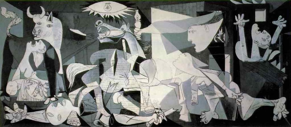
Figure 1. Art as an element in a global context. In Guernica, Pablo Picasso, by means of his own style built upon many artistic influences, such as Cubism or African art, expressed his emotions against war inspired by its historical and political context. Image source: www.PabloPicasso.org.

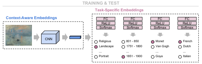
Figure 2. Overview of the Multi-Task Learning model.

In an attempt to analyse art from a global perspective, we propose to extract context-aware embeddings from paintings by considering both visual and contextual information. We propose two independent and separate models to encode contextual data in art. In the first one, a multi-task learning model (MTL) is used to capture visual relationships between artistic attributes in paintings. To do that, we optimise several artistic-related tasks jointly, so that the obtained generic embeddings are enforced to find common elements and hence, context, between the different tasks. In the second model, in contrast, we use a knowledge graph (KG) to learn the different relationships between artistic attributes. We create an art-specific KG by connecting a set of paintings with their artistic-related attributes. Then, node neighbourhoods and positions within the graph are encoded into a vector to represent context. Whereas the MTL model is able to capture relationships occurring at the visual-level, the use of KGs offers a more flexible representation of arbitrary relationships, which might not be well-structured and more difficult to detect when considering visual content only. In any case, we incorporate the information obtained with the aforementioned models into the art analysis system.

The two proposed context-aware embeddings are evaluated on the SemArt dataset (Garcia and Vogiatzis, 2018) in four different art classification tasks and in two cross-modal retrieval tasks. We show that, although none of the proposed models show a superior performance with respect to the other one in all of the evaluated tasks, context-aware embeddings consistently outperform methods based on visual embeddings only. Reported results show that performance is improved by up to 7.3% in art classification and a 37.24% in retrieval when our methods are used. In summary, our contributions are:

• To enhance standard visual features with contextual data in automatic art analysis.

• To propose a multi-task learning model to encode the visual relationships between different artistic attributes.

• To build an art-specific knowledge graph to capture contextual relationships between artistic attributes and use it to inform the visual model.

• To provide evidence that including contextual information improves performance in multiple art analysis tasks.

2. Related Work

Automatic Art Analysis. In order to identify specific attributes in paintings, early work in automatic art analysis was focused on representing the visual content of paintings by designing hand-crafted feature extraction methods (Johnson et al., 2008; Shamir et al., 2010; Carneiro et al., 2012; Khan et al., 2014; Mensink and Van Gemert, 2014). For example, (Johnson et al., 2008) proposed to detect authors by analysing their brushwork using wavelet decompositions, (Shamir et al., 2010; Khan et al., 2014) combined color, edge, or texture features for author, style, and school classification and (Carneiro et al., 2012; Mensink and Van Gemert, 2014) used SIFT features (Lowe, 2004) to classify paintings into different attributes.

In the last years, deep visual features extracted from CNNs have been repeatedly shown to be very effective in many computer vision tasks, including automatic art analysis (Bar et al., 2014; Karayev et al., 2014; Saleh and Elgammal, 2015; Tan et al., 2016; Ma et al., 2017; Mao et al., 2017; Garcia and Vogiatzis, 2018; Strezoski and Worring, 2018). At first, deep features were extracted from pre-trained networks and used off-the-shelf for automatic art classification (Bar et al., 2014; Karayev et al., 2014; Saleh and Elgammal, 2015). Later, deep visual features were shown to obtain better results when fine-tuned using painting images (Tan et al., 2016; Seguin et al., 2016; Mao et al., 2017; Strezoski and Worring, 2018; Chu and Wu, 2018). Alternatively, (Crowley et al., 2015; Crowley and Zisserman, 2014, 2016) explored domain transfer for object and face recognition in paintings, whereas (Garcia and Vogiatzis, 2018) introduced the use of joint visual and textual models to study paintings from a semantic perspective.

So far, most of the proposed methods in automatic art analysis have been focused on representing the visual essence of an artwork by capturing style and/or content. However, the study of art is not only about the visual appearance of paintings, but also about their historical, social, and artistic context. In this work, we propose to consider both visual and contextual information in art by introducing context-aware embeddings obtained by either a multi-task learning model or a knowledge graph.

Multi-Task Learning. Multi-task learning models (Caruana, 1997) aim to solve multiple tasks jointly with the hope that the generated generic features are more powerful than task-specific representations. In deep learning approaches, MTL is commonly performed via hard or soft parameter sharing (Ruder, 2017). Whereas in hard parameter sharing (Caruana, 1997; Sener and Koltun, 2018), except by the output layers, parameters are shared between all the tasks, in soft parameter sharing (Long and Wang, 2015; Yang and Hospedales, 2016), each task is defined by its own parameters, which are encouraged to remain similar via regularisation methods.

Following the success of MTL in many computer vision problems, such as object detection and recognition (Salakhutdinov et al., 2011; Bilen and Vedaldi, 2016), object tracking (Zhang et al., 2013), facial landmark detection (Zhang et al., 2014), or facial attribute classification (Rudd et al., 2016), we propose a hard parameter sharing MTL approach for obtaining context-aware embeddings in the domain of art analysis. In our approach, by jointly learning related artistic tasks, the resulting visual representations are enforced to capture relationships and common elements between the different artistic attributes, such as author, school, type, or period, and thus, providing contextual information about each painting.

Knowledge Graphs. Knowledge graphs are complex graph structures able to capture non-structured relationships between the data represented in the graph. When KGs are used to add contextual information to a multimedia database, prior work has shown consistent improvements in annotation, classification, and retrieval benchmarks (Fergus et al., 2010; Salakhutdinov et al., 2011; Chen et al., 2013; Deng et al., 2014; Johnson et al., 2015; Zhang et al., 2016; Marino et al., 2017; Cui et al., 2018; Wang et al., 2018).

To extract contextual information from a KG, one strategy is to encode relationships from visual concepts detected in pictures, forming concept hierarchies (Salakhutdinov et al., 2011; Deng et al., 2014). (Johnson et al., 2015) introduced human generated scene graphs based on descriptions of pictures to improve retrieval tasks, whereas (Cui et al., 2018) exploited semantic relationships between labels using ConceptNet (Speer and Havasi, 2012). Another strategy is to gather labelling information from social media to compute a word-image graph, in which random walks are proposed to extract topological information (Zhang et al., 2016). Other approaches incorporate the use of external knowledge bases. For example, (Fergus et al., 2010) proposed to improve classifiers with the use of WordNet (Miller, 1995), (Marino et al., 2017) designed an end-to-end learning pipeline to incorporate large knowledge graphs, such as Visual Genome (Krishna et al., 2016), into classification, and (Wang et al., 2018) trained image and graph embeddings using WordNet, NELL (Carlson et al., 2010), or NEIL (Chen et al., 2013).

While related work mostly rely on the use of external knowledge, in our knowledge graph model, we propose to capture contextual information only by processing the data provided with art datasets. As the semantic of art pieces is extremely domain specific, the symbolism that is implied in mythological or religious representations may not benefit from general knowledge. Instead, we leverage on metadata information from art datasets to create a domain-specific knowledge graph, from which we train context embeddings without any task-specific supervision.

3. Context-Aware Embeddings

We propose two independent models for capturing artistic context in paintings. In the first model, relationships between different artistic attributes are extracted from the visual appearance of images with a multi-task learning model, whereas in the second model, non-visual information extracted from artistic metadata is encoded by using knowledge graphs.

3.1. Multi-Task Learning Model

In the MTL model, artistic context is obtained by finding visual relationships between common elements in different artistic attributes. To compute context-aware embeddings, the model is trained to learn multiple artistic tasks jointly, so the generated embeddings are enforced to find visual similarities between the different tasks.

Formally, in a multi-task learning problem, given $T$ learning tasks, with the training setting for the $t$-th task consisting on $N_{t}$ training samples and denoted as $\{\vec{x}^{t}_{j},y^{t}_{j}\}^{N_{t}}_{j=1}$, where $\vec{x}^{t}_{j}\in\mathbb{R}^{d}$ and $y^{t}_{j}$ are the $j$-th training sample and its label, respectively, the goal is to optimise:

(1) $$\operatorname*{arg\,min}_{\{\vec{w}^{t}\}^{T}_{t=1}}\sum^{T}_{t=1}\sum^{N_{t}}_{j=1}\lambda^{t}\ell_{t}(f(\vec{x}_{j}^{t};\vec{w}^{t}),y_{j}^{t})$$

where $f$ is a function parameterised by the vector $\vec{w}^{t}$, $\ell_{t}$ is the loss function for the $t$-th task, and $\lambda^{t}$, with $\sum^{T}_{t=1}\lambda_{t}=1$, weights the contribution of each task.

In our model, we aim to distinguish between the context-aware information and the task-specific data. We define the function parameters for the $t$-th task as the contribution of two vectors, $\vec{w}^{t}=[\mathbf{w}_{g}^{t};\mathbf{w}_{s}^{t}]$, so that $f$ is defined as:

(2) $$f(\vec{x}_{j}^{t};\vec{w}^{t})=f_{s}(\mathbf{v}_{j}^{t};\mathbf{w}_{s}^{t})$$

where

(3) $$\mathbf{v}_{j}^{t}=f_{g}(\mathbf{x}_{j}^{t};\mathbf{w}_{g}^{t})$$

with $f_{g}$ being a context-aware function parametrised by $\mathbf{w}_{g}^{t}$, $f_{s}$ being a task-specific function parametrised by $\mathbf{w}_{s}^{t}$, and $\mathbf{v}_{j}^{t}$ being the $j$-th context-aware embedding generated by task $t$.

By sharing both the training data and the context-aware parameters across all the tasks as $\mathbf{x}_{j}^{t}=\mathbf{x}_{j}^{k}\text{ and }\mathbf{w}_{g}^{t}=\mathbf{w}_{g}^{k}\text{ for }j\neq k$, the context-aware embedding $\mathbf{v}_{j}^{t}$ is defined as:

(4) $$\mathbf{v}_{j}=f_{g}(\mathbf{x}_{j};\mathbf{w}_{g})$$

which enforces $\mathbf{v}_{j}$ to encode $\mathbf{x}_{j}$ in a generic and non task-specific representation by identifying patterns and relationships within different tasks. The problem, finally, is formulated as:

(5) $$\operatorname*{arg\,min}_{\mathbf{w}_{g},\{\vec{w}_{s}^{t}\}^{T}_{t=1}}\sum^{T}_{t=1}\sum^{N}_{j=1}\lambda^{t}\ell_{t}(f_{s}(f_{g}(\mathbf{x}_{j};\mathbf{w}_{g});\mathbf{w}_{s}^{t}),y_{j}^{t})$$

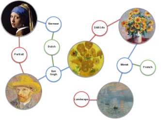
Figure 3. An example of our artistic KG. Each node corresponds to either a painting or an artistic attribute, whereas edges correspond to existing interconnections.

For solving this optimisation problem, we propose the model in Figure 2, in which the $T$ learning tasks correspond to multiple artistic classification challenges, such as type, school, timeframe, or author classification. To obtain context-aware embeddings, the context-aware function, $f_{g}$, is characterised by ResNet50 (He et al., 2016) after removing the last fully-connected layer, whereas the task-specific functions, $f_{s}$, are described by a fully connected layer followed by a ReLU non-linearity. The output of $f_{g}$ is a 2,048 dimensional embedding, which is input into the task-specific classifiers. Each classifier produces a $C_{t}$-dimensional task-specific embedding as output, $\mathbf{z}_{j}^{t}$, where $C_{t}$ is the number of classes in each task. Each tasks is formulated with the cross-entropy loss function as:

(6) $$\ell_{t}(\mathbf{z}_{j}^{t},y_{j}^{t})=-\log\Bigg{(}\frac{\exp(\mathbf{z}_{j}^{t}[y_{j}^{t}])}{\sum_{c}\exp(\mathbf{z}_{j}^{t}[c])}\Bigg{)}$$

where $\mathbf{z}_{j}^{t}=f_{s}(f_{g}(\mathbf{x_{j}};\mathbf{w}_{g});\mathbf{w}_{s}^{t})$.

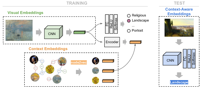
Figure 4. Overview of the Knowledge Graph model.

3.2. Knowledge Graph Model

In the MTL model, contextual information is provided by the painting images themselves by considering the relationships between common elements in the visual appearance of the images when multiple artistic tasks are trained together. In the knowledge graph model (KGM), in contrast, contextual information is obtained from capturing relationships in an artistic knowledge graph built with non-visual artistic metadata.

Artistic Knowledge Graph. A KG is a graph structure, $G=(V,E)$, in which the entities and their relations are represented by a collection of nodes, $V$, and edges, $E$, respectively. We use a KG to capture contextual knowledge and similarities in the semantic space formed by the graph, often referred to as homophily (Goyal and Ferrara, 2018).

To construct an artistic KG, one strategy is to connect paintings with edges when sharing a common attribute $a\in A$. However, the complexity of this approach is expensive, reaching the order of $|V|^{2}\times|A|$. Instead, we propose to connect paintings with their attributes in a much sparser manner. We consider multiple types of node: paintings, $P\subseteq V$, which represent the paintings themselves (e.g. Girl with a Pearl Earring), and each family, $\psi$, of attributes $A_{\psi}\subseteq V$, which represent artistic concepts (e.g. a type such as Portrait or an author such as Van Gogh). We use the training data from the SemArt dataset (Garcia and Vogiatzis, 2018), which contains 19,244 paintings labeled with the attributes Author, Title, Date, Technique, Type, School, and Timeframe to connect edges, $e=(V_{p},V_{q})\in E$, between painting nodes, $V_{p}$, and attribute nodes, $V_{q}\in A_{\psi}$, with $\psi\in\{\text{{Type}, {Timeframe}, {Author}}\}$, when an attribute exists in a painting. As School corresponds to an author’s school, we connect an edge, $e=(V_{a},V_{s})\in E$, between an author, $V_{a}$, and a school, $V_{s}$. We additionally enrich our graph with three other families of attributes, which are connected to painting nodes. From Technique, we extract Material, such as oil, and Support, such as 210x80cm. Also, by computing the most common $n$-grams in the titles, with $n$ up to three, we extract keywords from the title of each painting, such as Three Graces. In total, the resulting KG presents 33,148 nodes and 125,506 edges, with 3,166 authors, 618 materials, 26 schools, 8,899 supports, 22 timeframes, 10 types, and 1,163 keyword nodes. An example representation of our artistic graph is shown in Figure 3.

Training. At training time, visual and context embeddings are computed from the painting image and from the KG, respectively, and used to optimise the weights of the model. Our training model is depicted in Figure 4 and each of its parts are detailed below.

Visual Embeddings. Visual embeddings represent the visual appearance of paintings, containing information about the content and the style of the artwork. To obtain the visual embeddings, we use a ResNet50 (He et al., 2016) without the last fully connected layer.

Context Embeddings. Context embeddings encode the artistic context of an artwork by extracting data from the KG. For encoding the KG information into a vector representation, we adopt the node2vec model (Grover and Leskovec, 2016) because of its capacity to preserve a trade-off between homophily and structural equivalences, resulting in high performances in node classification tasks (Goyal and Ferrara, 2018). To capture node embeddings, node2vec operates skip-grams over random walks in the KG, and associates a vector representing the neighbourhood and the overall position of each node in the graph.

Classifier. The classifier takes as input the visual embedding and predicts the artistic attributes contained in the sample painting. We use different kinds of attribute classifiers, such as type, school, timeframe, or author. The classifier is composed of a fully connected layer followed by a ReLU non-linearity, and its output is used to compute a classification loss using a cross-entropy loss function:

(7) $$\ell_{c}(\mathbf{z}_{j},class_{j})=-\log\Bigg{(}\frac{\exp(\mathbf{z}_{j}[class_{j}])}{\sum_{i}\exp(\mathbf{z}_{j}[i])}\Bigg{)}$$

where $\mathbf{z}_{j}$ and $class_{j}$ are the output of the classifier and the assigned label of the attribute for the $j$-th training painting, respectively.

Encoder. The encoder module, which is composed of a single fully connected layer, is used to project the visual embeddings into the context embedding space. We compute the loss between the projected visual embedding, $\mathbf{p}_{j}$, and the context embedding, $\mathbf{u}_{j}$, of the $j$-training sample with a smooth L1 loss function:

(8) $$\ell_{e}(\mathbf{p}_{j},\mathbf{u}_{j})=\frac{1}{n}\sum_{i}\delta_{ji}$$

where

$$\delta_{ji}=\begin{cases}\frac{1}{2}(p_{ji}-u_{ji})^{2},&\text{if}\ |p_{ji}-u_{ji}|\leq 1\\ |p_{ji}-u_{ji}|-\frac{1}{2},&\text{otherwise}\end{cases}$$

being $p_{ji}$ and $u_{ji}$ the $i$-th elements in $\mathbf{p}_{j}$ and $\mathbf{u}_{j}$, respectively. To train the KGM, we compute the total loss function of the model as a combination of the losses obtained from the classifier and encoder modules:

(9) $$\mathcal{L}=\lambda_{c}\sum_{j=1}^{N}\ell_{c}(\mathbf{z}_{j},class_{j})+\lambda_{e}\sum_{j=1}^{N}\ell_{e}(\mathbf{p}_{j},\mathbf{u}_{j})$$

where $\lambda_{c}$ and $\lambda_{e}$ are parameters that weight the contribution of the classification and the encoder modules, respectively, and $N$ is the number of training samples.

Whereas the parameters of the context embeddings are learnt without supervision and frozen during the KGM training process, the loss score, $\mathcal{L}$, obtained from Equation (9) is backpropagated through the weights of the visual embedding module. This enforces ResNet50 to compute embeddings that are meaningful for artistic classification by decreasing $\ell_{c}$, while incorporating contextual information from the knowledge graph by minimizing $\ell_{e}$.

Context-Aware Embeddings. At test time, to obtain context-aware embeddings from unseen test samples, painting images are fed into the fine-tuned ResNet50 model. As context embeddings computed directly from the KG cannot be obtained for samples that are not contained as a node, the context embedding and the encoder modules are removed from the test model (Figure 4).

However, the ResNet50 network has been enforced during the training process to (1) capture relevant visual information to predict artistic attributes and (2) to incorporate contextual data from the KG in the visual embeddings. Therefore, the output embeddings from the fine-tuned ResNet50 are, indeed, context-aware embeddings.

4. Art Classification

We evaluated the two proposed methods in multiple art classification tasks, including author identification and type classification.

4.1. Implementation Details

In both of our proposed models, painting images are encoded into a vector representation by using ResNet50 (He et al., 2016) without the last fully connected layer. ReNet50 is initialised with its standard pre-trained weights for image classification, whereas the weights from the rest of the layers are initialised randomly. Images are scaled down to 256 pixels per side and randomly cropped into 224 $\times$ 224 patches. At training time, visual data is augmented by randomly flipping images horizontally. The size of the embeddings produced by ResNet50 is 2,048, whereas the dimensionality produced by node2vec is 128. We use stochastic gradient descent with a momentum of 0.9 and a learning rate of 0.001 as optimiser. The training is conducted in mini-batches of 28 samples, with a patience of 30 epochs. In the MTL model, $\lambda_{t}$ is set to 0.25 for all the tasks, whereas in the KGM approach, $\lambda_{c}$ is set to 0.9 and $\lambda_{c}$ to 0.1.

4.2. Evaluation Dataset

Most of the proposed datasets for art classification evaluation are either too small to train deep learning models (Carneiro et al., 2012; Khan et al., 2014; Crowley and Zisserman, 2014), do not provide multiple attributes per image (Karayev et al., 2014), or are not available to download at the time of writing this work (Mao et al., 2017). Thus, we decide to use the recently introduced SemArt dataset (Garcia and Vogiatzis, 2018), which was envisaged for cross-modal retrieval, and can be easily adapted for classification evaluation. The SemArt dataset is a collection of 21,384 painting images, from which 19,244 are used for training, 1,069 for validation and 1,069 for test. Each painting is associated with an artistic comment and the following attributes: Author, Title, Date, Technique, Type, School and Timeframe. We implement the following four tasks for art classification evaluation.

Type Classification. Using the attribute Type, each painting is classified according to 10 different common types of paintings: portrait, landscape, religious, study, genre, still-life, mythological, interior, historical and other.

School Classification. The School attribute is used to assign each painting to one of the schools of art that appear at least in ten samples in the training set: Italian, Dutch, French, Flemish, German, Spanish, English, Netherlandish, Austrian, Hungarian, American, Danish, Swiss, Russian, Scottish, Greek, Catalan, Bohemian, Swedish, Irish, Norwegian, Polish and Other. Paintings with a school different to those are assigned to the class Unknown. In total, there are 25 school classes.

Timeframe Classification. The attribute Timeframe, which corresponds to periods of 50 years evenly distributed between 801 and 1900, is used to classify each painting according to its creation date. We only consider timeframes with at least ten paintings in the training set, obtaining a total of 18 classes, which includes an Unknown class for timeframes out of the selection.

Author Identification. The Author attribute is used to classify paintings according to 350 different painters. Although the SemArt dataset provides 3,281 unique authors, we only consider the ones with at least ten paintings in the training set, including an Unknown class for painters not contained in the final selection.

4.3. Baselines

Our models are compared against the following baselines:

Pre-trained Networks. VGG16 (Simonyan and Zisserman, 2015), ResNet50 (He et al., 2016) and Res-Net152 (He et al., 2016) with their pre-trained weights learnt in natural image classification. To adapt the models for art classification, we modified the last fully connected layer to match the number of classes of each task. The weights of the last layer were initialised randomly and fine-tuned during training, whereas the weights of the rest of the network were frozen.

Fine-tuned Networks. VGG16 (Simonyan and Zisserman, 2015), ResNet50 (He et al., 2016) and Res-Net152 (He et al., 2016) networks were fine-tuned for each art classification task. As in the pre-trained models, the last layer was modified to match the number of classes in each task.

ResNet50+Attributes. The output of each fine-tuned classification model from above was concatenated to the output of a pre-trained ResNet50 network without the last fully connected layer. The result was a high-dimensional embedding representing the visual content of the image and its attribute predictions. The high-dimensional embedding was input into a last fully connected layer with ReLU to predict the attribute of interest. Only the weights from the pre-trained ResNet50 and the last layer were fine-tuned, whereas the weights of the attribute classifiers were frozen.

ResNet50+Captions. For each painting, we generated a caption using the captioning model from (Xu et al., 2015). Captions were represented by a multi-hot vector with a vocabulary size of 5,000 and encoded into a 512-dimensional embedding with a fully connected layer followed by an hyperbolic tangent or tanh activation. The caption embeddings were then concatenated to the output of a ResNet50 network without the last fully connected layer. The concatenated vector was fed into a fully connected layer with ReLU to obtain the prediction.

Table 1. Art Classification Results on SemArt Dataset.

Method	Type	School	TF	Author
VGG16 pre-trained	0.706	0.502	0.418	0.482
ResNet50 pre-trained	0.726	0.557	0.456	0.500
ResNet152 pre-trained	0.740	0.540	0.454	0.489
VGG16 fine-tuned	0.768	0.616	0.559	0.520
ResNet50 fine-tuned	0.765	0.655	0.604	0.515
ResNet152 fine-tuned	0.790	0.653	0.598	0.573
ResNet50+Attributes	0.785	0.667	0.599	0.561
ResNet50+Captions	0.799	0.649	0.598	0.607
MTL context-aware	0.791	0.691	0.632	0.603
KGM context-aware	0.815	0.671	0.613	0.615

4.4. Results Analysis

We measured classification performance in terms of accuracy, i.e. the ratio of correctly classified samples over the total number of samples. Results are provided in Table 1. In every task, the best accuracy was obtained when a context-aware embedding method, MTL or KGM, was used. The MTL model performed slightly better than the KGM in School and Timeframe tasks, whereas the KGM was the best in classifying Type and Author attributes. Unsurprisingly, the pre-trained models obtained the worst results among all the baselines, as they do not present enough discriminative power in the domain of art. Also, there was a clear improvement with respect to pre-trained baselines when the networks were fine-tuned, as already noted in previous work (Tan et al., 2016; Seguin et al., 2016; Mao et al., 2017; Strezoski and Worring, 2018). On the other hand, adding attributes or captions to the visual representations seemed to improve the accuracy, although not in all the scenarios, e.g., Timeframe was better classified with the fine-tuned ResNet50 model than with ResNet50+Attributes or ResNet50+Captions, whereas School was better classified with the fine-tuned ResNet50 than with ResNet50+Captions. This suggests that informing the model with extra information may be beneficial. When the data used to inform the model was contextual and obtained from capturing relationships in artistic attributes, accuracy was boosted, with improvements ranging from 3.16% to 7.3% with respect to fine-tunned networks and from 1.32% to 5.5% with respect to ResNet50+Attributes and ResNet50+Captions models.

5. Art Retrieval

We also evaluated the use of context-aware embeddings on art retrieval problems by incorporating context-aware embeddings into a cross-modal retrieval algorithm.

5.1. Implementation Details

As evaluation protocol, we used the SemArt dataset and its proposed Text2Art challenge, which consists of two cross-modal retrieval tasks: text-to-image and image-to-text. In text-to-image retrieval, given an artistic comment and its attributes, the goal is to find the correct painting within all the test paintings in the dataset. Similarly, in image-to-text retrieval, given a sample painting, the goal is to find the correct comment. Details on the dataset attributes and data splits are described in Section 4.2. We incorporate context-aware embeddings in a cross-modal retrieval model by adding the context-aware classifiers in the visual encoder module. Details of the cross-modal retrieval model are provided below.

Visual encoder: Painting images are scaled down to 256 pixels per side and randomly cropped into 224 $\times$ 224 patches. Then, paintings are fed into ResNet50, initialised with its standard pre-trained weights, to obtain a 1,000-dimensional vector, $\mathbf{h}_{\text{cnn}}$, from the last convolutional layer. At the same time, paintings are fed into a context-aware classifier (i.e. the MTL model from Figure 2 or the KGM model from Figure 4) to obtain a $c$-dimensional vector, $\mathbf{h}_{\text{att}}$, containing the predicted attributes, with $c$ being the number of output classes in the classifier. The final visual representation, $\mathbf{h}$, is then computed as $\mathbf{h}=\mathbf{h}_{\text{cnn}}\oplus\mathbf{h}_{\text{att}}$, where $\oplus$ is concatenation.

Comment and attribute encoder: We encode each comment as a term frequency - inverse document frequency (tf-idf) vector, $\mathbf{q}_{\text{com}}$, using a vocabulary of size 9,708, which is built with the alphabetic words that appear at least ten times in the training set. We encode titles as another tf-idf vector, $\mathbf{q}_{\text{tit}}$, with a vocabulary of size 9,092, which is built with the alphabetic words that appear in the titles of the training set. Additionally, we encode Type, School, Timeframe, or Author attributes using a $c$-dimensional one-hot vector, $\mathbf{q}_{\text{att}}$, with $c$ being the number of classes in each attribute. The final joint comment and attributes representation, $\mathbf{q}$, is computed as $\mathbf{q}=\mathbf{q}_{\text{com}}\oplus\mathbf{q}_{\text{tit}}\oplus\mathbf{q}_{\text{att}}$.

Cross-Modal Projections: To compute similarities between cross-modal data, the visual representation, $\mathbf{h}$, and the joint comment and attributes representation, $\mathbf{q}$, are projected into a common 128-dimensional space using the non-linear functions $f_{h}$ and $f_{q}$, respectively. The non-linear functions are implemented with a fully connected layer followed by tanh activation and a $\ell_{2}$-normalisation. Once projected into the common space, elements are retrieved according to their cosine similarity.

Table 2. Results on the Text2Art Challenge.

	Text-to-Image					Image-to-Text
Model	R@1	R@5	R@10	MR		R@1	R@5	R@10	MR
CML	0.144	0.332	0.454	14		0.138	0.327	0.457	14
CML*	0.164	0.384	0.505	10		0.162	0.366	0.479	12
AMD Type	0.114	0.304	0.398	17		0.125	0.280	0.398	16
AMD School	0.103	0.283	0.401	19		0.118	0.298	0.423	16
AMD TF	0.117	0.297	0.389	20		0.123	0.298	0.413	17
AMD Author	0.131	0.303	0.418	17		0.120	0.302	0.428	16
Res152 Type	0.178	0.383	0.525	9		0.165	0.364	0.491	11
Res152 School	0.192	0.386	0.507	10		0.163	0.364	0.484	12
Res152 TF	0.127	0.322	0.432	18		0.130	0.336	0.444	16
Res152 Author	0.236	0.451	0.572	7		0.204	0.440	0.535	8
MTL Type	0.145	0.358	0.474	12		0.150	0.350	0.475	12
MTL School	0.196	0.428	0.536	8		0.172	0.396	0.520	10
MTL TF	0.171	0.394	0.525	9		0.138	0.353	0.466	12
MTL Author	0.232	0.452	0.567	7		0.206	0.431	0.535	9
KGM Type	0.152	0.367	0.506	10		0.147	0.367	0.507	10
KGM School	0.162	0.371	0.483	12		0.156	0.355	0.483	11
KGM TF	0.175	0.399	0.506	10		0.148	0.360	0.472	12
KGM Author	0.247	0.477	0.581	6		0.212	0.446	0.563	7

The weights of the retrieval model, except from the context-aware classifier which is frozen, are trained using both positive (i.e. matching) and negative (i.e. non-matching) pairs of samples with the cosine margin loss function:

(10) $$\begin{split}\mathcal{L}(\mathbf{h}_{k},\mathbf{q}_{j})=\begin{cases}1-\text{sim}(f_{h}(\mathbf{h}_{k}),f_{q}(\mathbf{q}_{j})),&\text{if }k=j\\ \max(0,\text{sim}(f_{h}(\mathbf{h}_{k}),f_{q}(\mathbf{q}_{j}))-\Delta),&\text{if }k\neq j\end{cases}\end{split}$$

where sim is the cosine similarity between two vectors and $\Delta=0.1$ is the margin. We use Adam optimiser with learning rate 0.0001.

5.2. Results Analysis

Results are reported as median rank (MR) and recall rate at $K$ (R@K), with $K$ being 1, 5, and 10. MR is the value separating the higher half of the relevant ranking position amount all samples, i.e. the lower the better, whereas R@K is the rate of samples for which its relevant image is in the top $K$ positions of the ranking, i.e. the higher the better.

We report results of the proposed cross-modal retrieval model using the following context-aware classifiers: MTL-Type, MTL-Timframe, MTL-School, MTL-Author, KGM-Type, KGM-School, KGM-Timeframe, and KGM-Author, in which only the specified attribute is used. As a baseline of the proposed model, results when using fine-tuned ResNet152 instead of a context-aware classifier are also reported. Our methods are compared against previous work: CML (Garcia and Vogiatzis, 2018), which encodes comments and titles without attribute information, and AMD (Garcia and Vogiatzis, 2018), in which attributes are used at training time to learn the visual and textual projections. CML*, is a re-implementation of CML with slightly better results.

Results are summarised in Table 2. The KGM-Author model obtained the best results, improving previous state of the art, CML*, by a 37.24% in average. When comparing context-aware models, in agreement with classification results (Table 1), MTL performed better than KGM when using School whereas KGM was the best in Type and Author attributes. We also noted that concatenating the output of an attribute classifier as proposed (ResNet152, MTL, and KGM models) improved results considerably with respect to AMD. However, we observed a big difference in performance when using the different attributes, being Author and Type the best and the worst ones, respectively. A possible explanation for this phenomenon may lay in the difference on the number of classes of each attribute.

Finally, our best model, KGM-Author, was further compared against human evaluators. In the easy setup, evaluators were shown an artistic comment, a title, and the attributes Author, Type, School, and Timeframe and were asked to choose the most appropriate painting from a pool of ten random images. In the difficult setup, however, instead of random paintings, the images shown shared the same attribute Type. Results are provided in Table 3. Our model reached values closer to human accuracy than previous work, outperforming CML by a 10.67% in the easy task and a 9.67% in the difficult task.

Table 3. Comparison against human evaluation on Text2Art.

	Model	Land	Relig	Myth	Genre	Port	Total
Easy Set	CCA (Garcia and Vogiatzis, 2018)	0.708	0.609	0.571	0.714	0.615	0.650
	CML (Garcia and Vogiatzis, 2018)	0.917	0.683	0.714	1	0.538	0.750
	KGM Author	0.875	0.805	0.857	0.857	0.846	0.830
	Human	0.918	0.795	0.864	1	1	0.889
Difficult Set	CCA (Garcia and Vogiatzis, 2018)	0.600	0.525	0.400	0.300	0.400	0.470
	CML (Garcia and Vogiatzis, 2018)	0.500	0.875	0.600	0.200	0.500	0.620
	KGM Author	0.600	0.825	0.700	0.400	0.650	0.680
	Human	0.579	0.744	0.714	0.720	0.674	0.714

6. Discussion

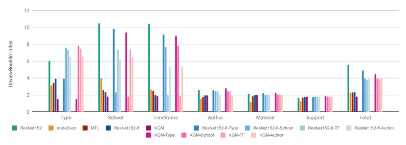
Figure 5. Davies-Bouldin index for each different attribute. The blue and red groups corresponds to single task of ResNet152-ft and KGM respectively. Their best results are reported in both ResNet152-ft and KGM columns of the first group.

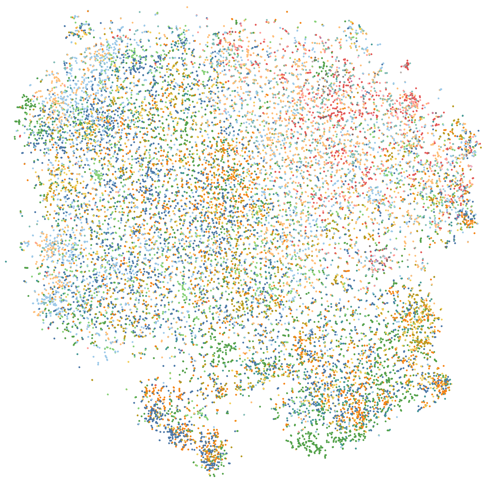
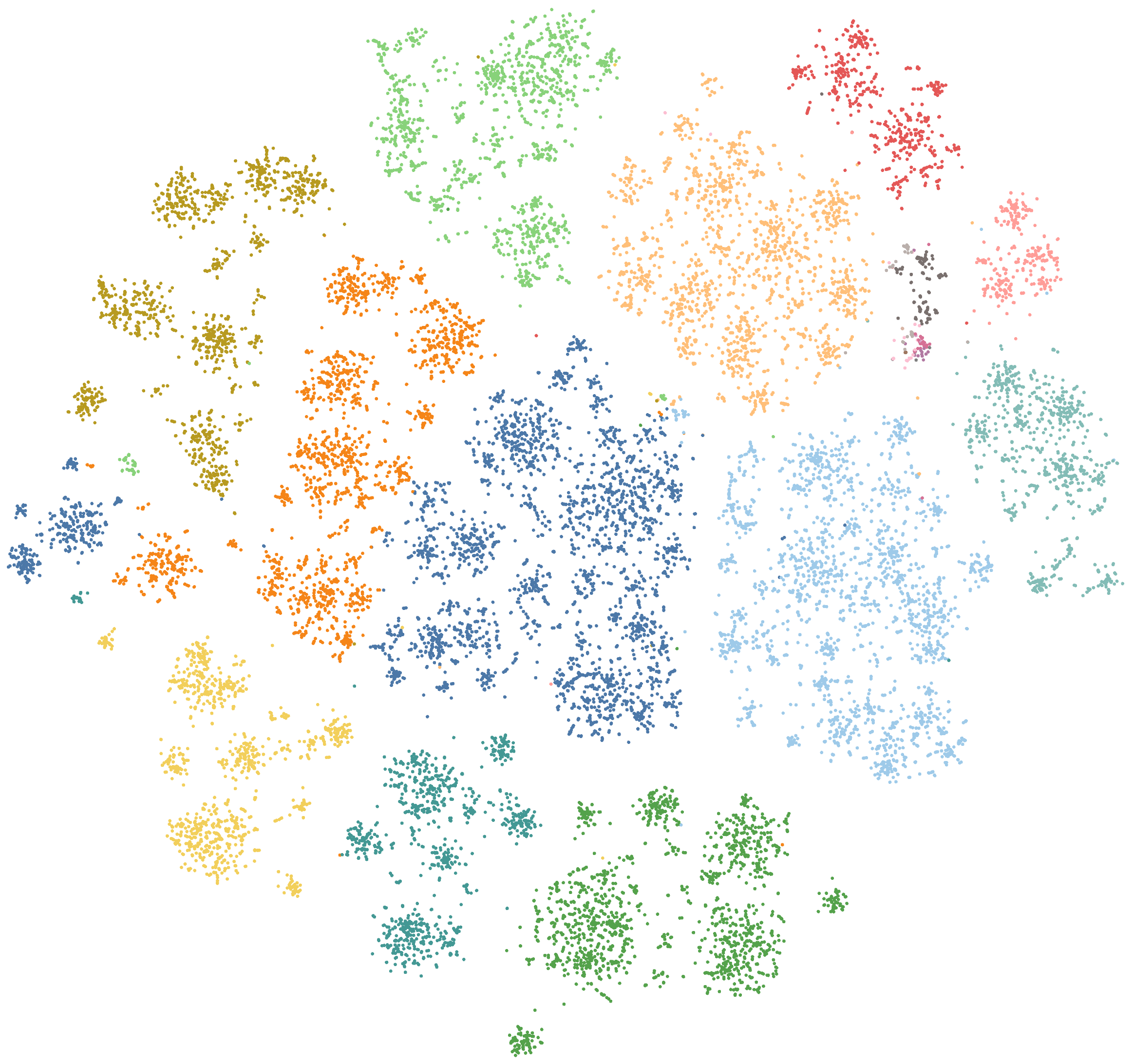
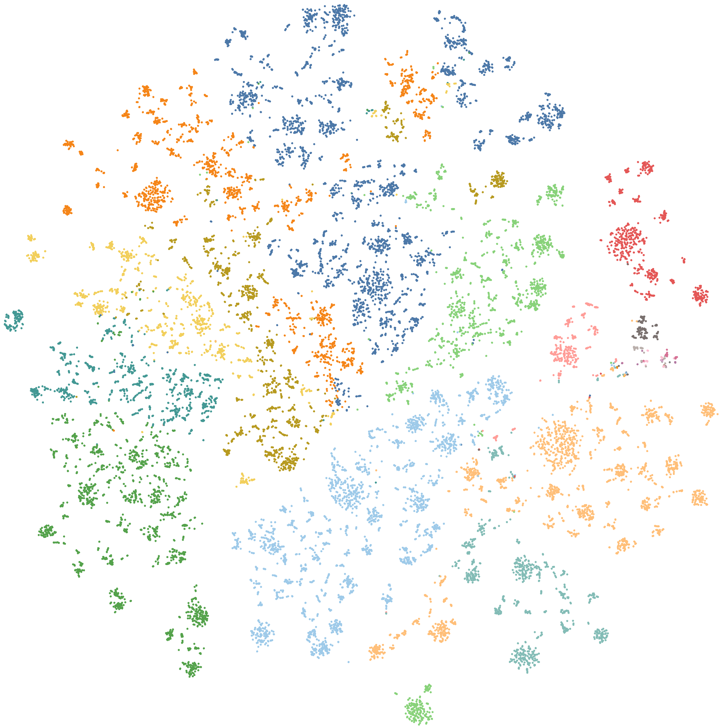
(a) ResNet152 pre-trained	(b) node2vec	(c) MTL

Figure 6. Embeddings of paintings projected in Tulip (Auber et al., 2017) using $t-$SNE (Wattenberg et al., 2016). Each node is a painting and the colouring is mapped to the Timeframe attribute. There is good separability of Timeframe values in the node2vec and MTL, as opposed to ResNet152.

So far, we have presented different models to capture contextual information in art, reporting results in art classification and retrieval tasks. However, further discussion about the quality of the contextual embeddings is required. In this section, we study how well context is captured in different types of embeddings by analysing the separability of artistic attributes in clusters.

To estimate the separability between clusters, we applied the Davies-Bouldin index (Davies and Bouldin, 1979), $Q$, which measures a trade-off between dispersion, $S_{i}$, and separation, $D_{ij}$, of the clusters $i$ and $j$:

(11) $$Q=\frac{1}{k}\sum_{i=1}^{k}\left(\max_{i\neq j}\left(\frac{S_{i}+S_{j}}{D_{ij}}\right)\right)$$

where $k$ is the number clusters, and $S_{i}$ and $D_{ij}$ are computed as:

$$S_{i}=\left(\frac{1}{|C_{i}|}\sum_{\mathbf{x}\in C_{i}}{\|\mathbf{x}-A_{i}\|^{p}}\right)^{1/p}\qquad D_{ij}=\|A_{i}-A_{j}\|_{p}$$

being $A_{i}$ the centroid of cluster $i$ of element $\mathbf{x}\in C_{i}$ computed using the $\ell_{p}$ distance, and $|C_{i}|$ the number of elements in $C_{i}$.

To compare the different settings, we used the samples from the training set and we applied $Q$ with $p=2$ to multiple types of embeddings on different attributes, as reported in Figure 5. When compared on the same task, the smaller value of $Q$, the better the cluster separation tends to be. We used Type, School, Timeframe, and Author attributes to compare performances between models. We also included the derived Material and Support attributes, for which none of our models was fine-tuned. Along with Author, these new attributes have the highest dispersion due to their large number of classes, showing the lowest $Q$ values.

The compared embeddings are detailed in Figure 5. The pre-trained ResNet152 baseline (in green) shows consistently the worst results in most categories, whereas the node2vec baseline trained on our KG (in orange) shows a good trade-off between categories and the best performance on the most complex attributes Author, Material and Support. On average, KGM (in purple) performs the best due to its high quality on each of the Type, School, and Timeframe attributes for which it has been trained. On average, the MTL (in red) shows a comparable performance to the multiple single-task fine-tuned ResNet152 (in blue).

These results rule in favour of the added value that contextual knowledge brought by the KG improves overall performances. We may further confirm this intuition from the 2D-projected embeddings in Figure 6: while the space represented by pre-trained ResNet152 applied to art does not show any convincing separability, the subspace formed by paintings in the node2vec embeddings shows clear separability and sub-densities. MTL does display such a structure, while being much more fractioned. Although intriguing, the analysis of these clusters’ content and how they may capture abstract concepts of art is a discussion we leave for future work.

7. Conclusions

This work proposed the use of context-aware embeddings for art classification and retrieval problems. Two methods for obtaining context-aware embeddings were introduced. The first one, based on multi-task learning, captures the relationships between visual artistic elements in paintings, whereas the second one, based on knowledge graphs, encodes the interconnections between non-visual artistic attributes. The reported results showed that context-aware embeddings are beneficial in many automatic art analysis problems, improving art classification accuracy by up to a 7.3% with respect to classification baselines. In cross-modal retrieval tasks, our best model outperforms previous work by a 37.24%. Future work will study the combination of multi-task learning and knowledge graphs into a single context-aware framework.

- (1)
- Auber et al. (2017) David Auber, Daniel Archambault, Romain Bourqui, Maylis Delest, Jonathan Dubois, Antoine Lambert, Patrick Mary, Morgan Mathiaut, Guy Mélançon, Bruno Pinaud, Benjamin Renoust, and Jason Vallet. 2017. TULIP 5. In Encyclopedia of Social Network Analysis and Mining. Springer, 1–28.
- Bar et al. (2014) Yaniv Bar, Noga Levy, and Lior Wolf. 2014. Classification of Artistic Styles Using Binarized Features Derived from a Deep Neural Network. In ECCV Workshops.
- Bilen and Vedaldi (2016) Hakan Bilen and Andrea Vedaldi. 2016. Integrated perception with recurrent multi-task neural networks. In Advances in neural information processing systems. 235–243.
- Carlson et al. (2010) Andrew Carlson, Justin Betteridge, Bryan Kisiel, Burr Settles, Estevam R Hruschka Jr, and Tom M Mitchell. 2010. Toward an architecture for never-ending language learning.. In AAAI, Vol. 5. Atlanta, 3.
- Carneiro et al. (2012) Gustavo Carneiro, Nuno Pinho da Silva, Alessio Del Bue, and João Paulo Costeira. 2012. Artistic image classification: An analysis on the printart database. In ECCV.
- Caruana (1997) Rich Caruana. 1997. Multitask learning. Machine learning 28, 1 (1997), 41–75.
- Chen et al. (2013) Xinlei Chen, Abhinav Shrivastava, and Abhinav Gupta. 2013. Neil: Extracting visual knowledge from web data. In Proceedings of the IEEE International Conference on Computer Vision. 1409–1416.
- Chu and Wu (2018) Wei-Ta Chu and Yi-Ling Wu. 2018. Image style classification based on learnt deep correlation features. IEEE Transactions on Multimedia 20, 9 (2018), 2491–2502.
- Collomosse et al. (2017) John Collomosse, Tu Bui, Michael J Wilber, Chen Fang, and Hailin Jin. 2017. Sketching with Style: Visual Search with Sketches and Aesthetic Context.. In ICCV. 2679–2687.
- Crowley and Zisserman (2014) Elliot Crowley and Andrew Zisserman. 2014. The State of the Art: Object Retrieval in Paintings using Discriminative Regions.. In BMVC.
- Crowley et al. (2015) Elliot J Crowley, Omkar M Parkhi, and Andrew Zisserman. 2015. Face Painting: querying art with photos.. In BMVC. 65–1.
- Crowley and Zisserman (2016) Elliot J Crowley and Andrew Zisserman. 2016. The art of detection. In ECCV. Springer.
- Cui et al. (2018) Peng Cui, Shaowei Liu, and Wenwu Zhu. 2018. General Knowledge Embedded Image Representation Learning. IEEE Transactions on Multimedia 20, 1 (2018), 198–207.
- Davies and Bouldin (1979) David L Davies and Donald W Bouldin. 1979. A cluster separation measure. IEEE transactions on pattern analysis and machine intelligence 2 (1979), 224–227.
- Deng et al. (2014) Jia Deng, Nan Ding, Yangqing Jia, Andrea Frome, Kevin Murphy, Samy Bengio, Yuan Li, Hartmut Neven, and Hartwig Adam. 2014. Large-scale object classification using label relation graphs. In European conference on computer vision. Springer, 48–64.
- Fergus et al. (2010) Rob Fergus, Hector Bernal, Yair Weiss, and Antonio Torralba. 2010. Semantic label sharing for learning with many categories. In European Conference on Computer Vision. Springer, 762–775.
- Garcia and Vogiatzis (2018) Noa Garcia and George Vogiatzis. 2018. How to Read Paintings: Semantic Art Understanding with Multi-Modal Retrieval. In Proceedings of the European Conference in Computer Vision Workshops.
- Goyal and Ferrara (2018) Palash Goyal and Emilio Ferrara. 2018. Graph embedding techniques, applications, and performance: A survey. Knowledge-Based Systems 151 (2018), 78–94.
- Grover and Leskovec (2016) Aditya Grover and Jure Leskovec. 2016. node2vec: Scalable feature learning for networks. In Proceedings of the 22nd ACM SIGKDD international conference on Knowledge discovery and data mining. ACM, 855–864.
- He et al. (2016) Kaiming He, Xiangyu Zhang, Shaoqing Ren, and Jian Sun. 2016. Deep residual learning for image recognition. In Proceedings of the IEEE conference on computer vision and pattern recognition.
- Johnson et al. (2008) C Richard Johnson, Ella Hendriks, Igor J Berezhnoy, Eugene Brevdo, Shannon M Hughes, Ingrid Daubechies, Jia Li, Eric Postma, and James Z Wang. 2008. Image processing for artist identification. IEEE Signal Processing Magazine 25, 4 (2008).
- Johnson et al. (2015) Justin Johnson, Ranjay Krishna, Michael Stark, Li-Jia Li, David Shamma, Michael Bernstein, and Li Fei-Fei. 2015. Image retrieval using scene graphs. In Proceedings of the IEEE conference on computer vision and pattern recognition. 3668–3678.
- Karayev et al. (2014) Sergey Karayev, Matthew Trentacoste, Helen Han, Aseem Agarwala, Trevor Darrell, Aaron Hertzmann, and Holger Winnemoeller. 2014. Recognizing Image Style. In BMVC.
- Khan et al. (2014) Fahad Shahbaz Khan, Shida Beigpour, Joost Van de Weijer, and Michael Felsberg. 2014. Painting-91: a large scale database for computational painting categorization. Machine vision and applications (2014).
- Krishna et al. (2016) Ranjay Krishna, Yuke Zhu, Oliver Groth, Justin Johnson, Kenji Hata, Joshua Kravitz, Stephanie Chen, Yannis Kalantidis, Li-Jia Li, David A Shamma, Michael Bernstein, and Li Fei-Fei. 2016. Visual Genome: Connecting Language and Vision Using Crowdsourced Dense Image Annotations. https://arxiv.org/abs/1602.07332
- Krizhevsky et al. (2012) Alex Krizhevsky, Ilya Sutskever, and Geoffrey E Hinton. 2012. Imagenet classification with deep convolutional neural networks. In NIPS.
- Long and Wang (2015) Mingsheng Long and Jianmin Wang. 2015. Learning multiple tasks with deep relationship networks. CoRR, abs/1506.02117 3 (2015).
- Lowe (2004) David G Lowe. 2004. Distinctive image features from scale-invariant keypoints. International journal of computer vision 60, 2 (2004), 91–110.
- Ma et al. (2017) Daiqian Ma, Feng Gao, Yan Bai, Yihang Lou, Shiqi Wang, Tiejun Huang, and Ling-Yu Duan. 2017. From Part to Whole: Who is Behind the Painting?. In Proceedings of the 2017 ACM on Multimedia Conference. ACM.
- Mao et al. (2017) Hui Mao, Ming Cheung, and James She. 2017. DeepArt: Learning Joint Representations of Visual Arts. In ACM on Multimedia Conference.
- Marino et al. (2017) Kenneth Marino, Ruslan Salakhutdinov, and Abhinav Gupta. 2017. The More You Know: Using Knowledge Graphs for Image Classification. In 2017 IEEE Conference on Computer Vision and Pattern Recognition (CVPR). IEEE, 20–28.
- Mensink and Van Gemert (2014) Thomas Mensink and Jan Van Gemert. 2014. The rijksmuseum challenge: Museum-centered visual recognition. In ICMR.
- Miller (1995) George A Miller. 1995. WordNet: a lexical database for English. Commun. ACM 38, 11 (1995), 39–41.
- Rudd et al. (2016) Ethan M Rudd, Manuel Günther, and Terrance E Boult. 2016. Moon: A mixed objective optimization network for the recognition of facial attributes. In European Conference on Computer Vision. Springer, 19–35.
- Ruder (2017) Sebastian Ruder. 2017. An overview of multi-task learning in deep neural networks. arXiv preprint arXiv:1706.05098 (2017).
- Salakhutdinov et al. (2011) Ruslan Salakhutdinov, Antonio Torralba, and Josh Tenenbaum. 2011. Learning to share visual appearance for multiclass object detection. In Computer Vision and Pattern Recognition (CVPR), 2011 IEEE Conference on. IEEE, 1481–1488.
- Saleh and Elgammal (2015) Babak Saleh and Ahmed M. Elgammal. 2015. Large-scale Classification of Fine-Art Paintings: Learning The Right Metric on The Right Feature. CoRR (2015).
- Sanakoyeu et al. (2018) Artsiom Sanakoyeu, Dmytro Kotovenko, Sabine Lang, and Björn Ommer. 2018. A Style-Aware Content Loss for Real-time HD Style Transfer. In Proceedings of the European Conference on Computer Vision, Vol. 2.
- Seguin et al. (2016) Benoit Seguin, Carlotta Striolo, Frederic Kaplan, et al. 2016. Visual link retrieval in a database of paintings. In ECCV Workshops.
- Sener and Koltun (2018) Ozan Sener and Vladlen Koltun. 2018. Multi-task learning as multi-objective optimization. In Advances in Neural Information Processing Systems. 525–536.
- Shamir et al. (2010) Lior Shamir, Tomasz Macura, Nikita Orlov, D Mark Eckley, and Ilya G Goldberg. 2010. Impressionism, expressionism, surrealism: Automated recognition of painters and schools of art. ACM Transactions on Applied Perception (2010).
- Simonyan and Zisserman (2015) K. Simonyan and A. Zisserman. 2015. Very Deep Convolutional Networks for Large-Scale Image Recognition. In International Conference on Learning Representations.
- Speer and Havasi (2012) Robert Speer and Catherine Havasi. 2012. Representing General Relational Knowledge in ConceptNet 5.. In LREC. 3679–3686.
- Strezoski and Worring (2018) Gjorgji Strezoski and Marcel Worring. 2018. OmniArt: A Large-scale Artistic Benchmark. ACM Transactions on Multimedia Computing, Communications, and Applications (TOMM) 14, 4 (2018), 88.
- Tan et al. (2016) Wei Ren Tan, Chee Seng Chan, Hernán E. Aguirre, and Kiyoshi Tanaka. 2016. Ceci n’est pas une pipe: A deep convolutional network for fine-art paintings classification. ICIP (2016).
- Wang et al. (2018) Xiaolong Wang, Yufei Ye, and Abhinav Gupta. 2018. Zero-shot Recognition via Semantic Embeddings and Knowledge Graphs. In Proceedings of the IEEE Conference on Computer Vision and Pattern Recognition. 6857–6866.
- Wattenberg et al. (2016) Martin Wattenberg, Fernanda Viégas, and Ian Johnson. 2016. How to Use t-SNE Effectively. Distill (2016). https://doi.org/10.23915/distill.00002
- Xu et al. (2015) Kelvin Xu, Jimmy Ba, Ryan Kiros, Kyunghyun Cho, Aaron Courville, Ruslan Salakhudinov, Rich Zemel, and Yoshua Bengio. 2015. Show, attend and tell: Neural image caption generation with visual attention. In International conference on machine learning. 2048–2057.
- Yang and Hospedales (2016) Yongxin Yang and Timothy Hospedales. 2016. Deep multi-task representation learning: A tensor factorisation approach. arXiv preprint arXiv:1605.06391 (2016).
- Zhang et al. (2016) Hanwang Zhang, Xindi Shang, Huanbo Luan, Meng Wang, and Tat-Seng Chua. 2016. Learning from Collective Intelligence: Feature Learning Using Social Images and Tags. ACM Trans. Multimedia Comput. Commun. Appl. 13, 1, Article 1 (Nov. 2016), 23 pages. https://doi.org/10.1145/2978656
- Zhang et al. (2013) Tianzhu Zhang, Bernard Ghanem, Si Liu, and Narendra Ahuja. 2013. Robust visual tracking via structured multi-task sparse learning. International journal of computer vision 101, 2 (2013), 367–383.
- Zhang et al. (2014) Zhanpeng Zhang, Ping Luo, Chen Change Loy, and Xiaoou Tang. 2014. Facial landmark detection by deep multi-task learning. In European Conference on Computer Vision. Springer, 94–108.