The stellar halo of the Milky Way traced by blue horizontal-branch stars in the Subaru Hyper Suprime-Cam Survey

Abstract

We report on the global structure of the Milky Way (MW) stellar halo up to its outer boundary based on the analysis of blue-horizontal branch stars (BHBs). These halo tracers are extracted from the $(g,r,i,z)$ band multi-photometry in the internal data release of the on-going Hyper Suprime-Cam Subaru Strategic Program (HSC-SSP) surveyed over $\sim 550$ deg² area. In order to select most likely BHBs by removing blue straggler stars (BSs) and other contamination in a statistically significant manner, we have developed and applied an extensive Bayesian method, instead of the simple color cuts adopted in our previous work, where each of the template BHBs and non-BHBs obtained from the available catalogs is represented as a mixture of multiple Gaussian distributions in the color-color diagrams. We found from the candidate BHBs in the range of $18.5<g<23.5$ mag that the radial density distribution over a Galactocentric radius of $r=36-360$ kpc can be approximated as a single power-law profile with an index of $\alpha=3.74^{+0.21}_{-0.22}$ or a broken power-law profile with an index of $\alpha_{\rm in}=2.92^{+0.33}_{-0.33}$ at $r$ below a broken radius of $r_{\rm b}=160^{+18}_{-19}$ kpc and a very steep slope of $\alpha_{\rm out}=15.0^{+3.7}_{-4.5}$ at $r>r_{\rm b}$. The latter profile with a prolate shape having an axial ratio of $q=1.72^{+0.44}_{-0.28}$ is most likely and this halo may hold a rather sharp boundary at $r\simeq 160$ kpc. The slopes of the halo density profiles are compared with those from the suite of hydrodynamical simulations for the formation of stellar halos. This comparison suggests that the MW stellar halo may consist of the two overlapping components: the in situ. inner halo as probed by RR Lyrae stars showing a relatively steep radial density profile and the ex situ. outer halo with a shallow profile probed by BHBs here, which is made by accretion of small stellar systems.

1 Introduction

A stellar halo surrounding a disk galaxy like our Milky Way (MW) is thought to have been developed through hierarchical assembly of small stellar systems such as dwarf galaxies (Searle & Zinn, 1978). Because of the long relaxation time in the halo, the structure of a current stellar halo, including the distribution of both smooth and non-smooth spatial features, reflects the past merging and accretion histories. Indeed, many halo substructures have been identified in the form of stellar streams in spatial coordinates as well as separate clumps in phase space. The former substructures correspond to the merging events within a few dynamical times, whereas the latter ones in phase space persist over many billion years (e.g., Helmi & White (1999); Bullock & Johnston (2005); Cooper et al. (2010)).

The smooth component of a stellar halo is also affected by the past merging history. Deason et al. (2014) investigated the results of numerical simulation for the merging-driven formation of a stellar halo by Bullock & Johnston (2005) and showed that the slope of the density profile for the outer part of a stellar halo depends on the average time of merging, in such a manner that the case of a more recent merging time reveals a shallower radial density profile over $50<r/{\rm kpc}<100$. It is also shown that the break in the stellar halo slope, which might be present in the MW halo, can be made by tidal debris from a merging satellite when it is at an apocenter position (Deason et al., 2018b). Also, the recent suite of magneto-hydrodynamical numerical simulation for galaxy formation, named Auriga (Grand et al., 2017; Monachesi et al., 2018), shows that both the slope in a density profile of a simulated stellar halo and its metallicity gradient are intimately related to the number of main progenitor satellites, which contribute to the total mass of a final halo. It is thus of great importance to derive the structure of a stellar halo to infer its merging history.

While the detection and analysis of stellar halos in external disk galaxies are challenging because of their very faint brightness, the stars distributed in the MW halo provide us with a unique opportunity to study the structure of the stellar halo in great detail (see reviews, Helmi (2008); Ivezić, Beers & Juric (2012); Feltzing & Chiba (2013); Bland-Hawthorn & Freeman (2014)). The direct method probing the MW stellar halo is to use bright halo tracers including red giant-branch (RGB) stars, RR Lyrae (RRL), blue horizontal-branch (BHB) stars as well as blue straggler (BS) stars, with which it is possible to map out the MW stellar halo out to its outer part (e.g., Sluis & Arnold (1998); Yanny et al. (2000); Chen et al. (2001); Sirko et al. (2004); Newberg & Yanny (2005); Jurić et al. (2008); Keller et al. (2008); Sesar et al. (2011); Deason et al. (2011); Xue et al. (2011); Deason et al. (2014); Cohen et al. (2015, 2017); Vivas et al. (2016); Slater et al. (2016); Xu et al. (2018); Hernitschek et al. (2018)). These studies over a Galactocentric distance $r$ of a few tens kpc to $\sim 100$ kpc have revealed that the MW stellar halo includes a general smooth component, which is often fit to a power-law density profile, and several irregular substructures associated with recent merging events of dwarf galaxies, such as the Sagittarius stream and Virgo overdensity (Ibata et al., 1995; Belokurov et al., 2006; Jurić et al., 2008).

More recent studies have explored much distant halo regions beyond $r=100$ kpc to reach a possible virial radius of a MW-sized dark matter halo with $r\sim 300$ kpc and more (Hernitschek et al., 2018; Deason et al., 2018a; Fukushima et al., 2018; Thomas et al., 2018). This is because the outer parts of a stellar halo reflect the merging/accretion history over past billion years (Bullock & Johnston, 2005; Deason et al., 2014; Pillepich et al., 2014; Monachesi et al., 2018). In particular, the outer boundary of the stellar halo may be present in the form of a sharp outer edge or broadly extended without any clear cut depending on the recent merging/accretion events. Among several halo tracers to probe the outskirts of the MW stellar halo, BHB stars have been frequently adopted and analyzed in the large photometric surveys including Subaru/Hyper Suprime-Cam (HSC) (Deason et al., 2018a; Fukushima et al., 2018) and Canada-France Imaging Survey (CFIS) (Thomas et al., 2018). Deason et al. (2018a) selected BHBs from the public data release of the HSC Subaru Strategic Program (HSC-SSP) surveyed over $\sim 100$ deg² using $griz$-band photometry and derived the power-law radial profile with an index $\alpha\simeq 4$. Concurrently with the completion of this work, we elsewhere reported (Fukushima et al., 2018) our results using BHBs extracted from the internal data release of HSC-SSP over $\sim 300$ deg². They derived a halo density profile between $r=50$ kpc and 300 kpc and fit, after the subtraction of the fields containing known substructures, to either a single power-law model with $\alpha\simeq 3.5$ and an axial ratio of $q\simeq 1.3$ or a broken power-law model with an inner/outer slope of $3.2/5.3$ at a break radius of 210 kpc. More recently, Thomas et al. (2018) presented their analysis of BHBs selected using deep $u$-band imaging from the CFIS survey combined with $griz$-band data from Pan-STARRS 1. They show that a broken power-law model with an inner/outer slope of $4.24/3.21$ at a break radius of 41.4 kpc is the best fitting case out to $r\sim 220$ kpc.

The main obstacle in the selection of BHBs from photometric data is to remove the contaminants having similar colors and magnitudes to BHBs, such as BSs, white dwarfs (WDs), QSOs, as well as distant faint galaxies having point-source images. This issue is more important in the outer parts of the halo, where the number density of BHBs becomes quite sparse compared with the contaminants. In our previous work (Fukushima et al., 2018), we use the HSC-SSP data obtained until 2016 April (internal data release S16A) and select BHBs located inside specific regions in the color-color diagrams defined in the combination of $griz$ band. This selection method of BHBs based on the simple color cuts provides basically the same results as those based on the maximum likelihood method, where the probability distribution of each stellar population is given as a single Gaussian in $griz$ space (see also Deason et al. (2018a)). The current paper is an extension of our previous work, in which we use the most recent internal data release of HSC-SSP covering $\sim 550$ deg² and develop an extensive Bayesian method to minimize the effects of non-BHB contamination as much as possible. We also consider the distribution of BS stars to obtain the additional information on the structure of the MW stellar halo.

This paper is organized as follows. In Section 2, we present the data that we utilize here and the method for the selection of candidate BHBs based on the $griz$-band photometric data obtained in the HSC-SSP survey. Our Bayesian method for the selection of BHB stars and their spatial distribution is also described. In Section 3, we show the results and discussion of our Bayesian analysis for the best set of parameters of the spatial distribution of BHB stars. Our conclusions are drawn in Section 4.

Obseved Regions with HSC-SSP Region RA DEC $l$ $b$ Adopted area Use (deg) (deg) (deg) (deg) (deg²) Yes/No XMM-LSS 35 $-5$ 170 $-59$ 60 No WIDE12H 180 0 276 60 68 Yes WIDE01H 19 0 136 $-62$ 0 No VVDS 337 0 65 $-46$ 169 Yes GAMA15H 217 0 347 54 85 No GAMA09H 135 0 228 28 92 Yes HECTOMAP 242 43 68 47 75 Yes AEGIS 214 51 95 60 2.5 Yes

2 Data and Method

2.1 Data

We make use of the imaging data obtained from the HSC-SSP Wide survey, which plans to cover $\sim 1,400$ deg² in five photometric bands ($g$, $r$, $i$, $z$, and $y$) (Aihara et al., 2018a, b; Furusawa et al., 2018; Kawanomoto et al., 2018; Komiyama et al., 2018; Miyazaki et al., 2018). In this Wide layer, the target 5$\sigma$ point-source limiting magnitudes are ($g$, $r$, $i$, $z$, $y$) = (26.5, 26.1, 25.9, 25.1, 24.4) mag. In this work, we adopt the $g$, $r$, $i$ and $z$-band data obtained before 2018 April (internal data release S18A), for the selection of BHBs and the removal of other contaminants as explained below. The data set covers six separate fields along the celestial equator, named XMM-LSS, WIDE12H, WIDE01H, VVDS, GAMA15H and GAMA09H, a field named HECTOMAP around $(\alpha_{\rm 2000},\delta_{\rm 2000})=(242^{\circ},43^{\circ})$, and a calibration field named AEGIS around $(240^{\circ},51^{\circ})$, amounting to $\sim 550$ deg² in total (See Table 1). Since WIDE01H has no $i$ and $z$-band data, we do not use this region. The total area that the current data set covers is to be compared with $\sim 300$ deg² covered in our previous analysis of BHBs from the data obtained before 2016 April (Fukushima et al., 2018). The HSC data are processed with hscPipe v6.5 (Bosch et al., 2018), a branch of the Large Synoptic Survey Telescope pipeline (Ivezić et al., 2008; Axelrod et al., 2010; Jurić et al., 2017) calibrated against PS1 DR1 photometry and astrometry (Schlafly et al., 2012; Tonry et al., 2012; Magnier et al., 2013). All the photometry data are corrected for the mean Galactic foreground extinction (Schlafly & Finkbeiner, 2011).

We note that as shown in Fukushima et al. (2018), both GAMA15H and XMM-LSS contain several spatial substructures associated with the Sagittarius (Sgr) stream, which is formed from a tidally disrupting, polar-orbit satellite, Sgr dwarf. Our interest in this paper is to deduce the structure of the smooth halo component, thus we exclude these fields in the following analysis.

2.2 Selection of targets

For the analysis of BHBs from our current sample, we select point sources using the extendedness parameter from the pipeline, namely extendedness$=0$ for point sources and extendedness$=1$ for extended images like galaxies. This parameter is computed based on the ratio between PSF and cmodel fluxes (Abazajian et al., 2004), where a point source is defined to be an object having this ratio larger than 0.985. As shown in Aihara et al. (2018b), this star/galaxy classification becomes uncertain for faint sources. The contamination, defined as the fraction of galaxies classified as HST/ACS among HSC-classified stars, is close to zero at $i<23$, but increases to $\sim 50\%$ at $i=24.5$ at the median seeing of the survey ($0.7$ arcsec). These properties are summarized in Figure 1. In what follows, we adopt point sources with $i\leq 24.5$ and investigate the possible effect of the contamination by faint galaxies.

Figure 1: The circles denote the fraction of stars classified as HST/ACS among HSC-classified stars for three different seeings of $0^{\prime\prime}.67$, $0^{\prime\prime}.57$ and $0^{\prime\prime}.52$. This fraction is close to one at $i<23$ and decreases to $\sim 0.5$ at $i=24.5$ at the high seeing of the survey ($0^{\prime\prime}.67$). The lines show the fitted functions given in Equation (3).

We then select point sources in the following magnitude and color ranges:

$$18.5< g <23.5$$

$$-0.3<g - r<0$$

$$-0.4<r - i<0.4$$

$$-0.25<i - z<0.1\ ,$$ (1)

where the faint limit for the $g$-band magnitude range is taken based on its photometric error of typically $\simeq 0.05$ mag with maximum of $\simeq 0.1$ mag

These point-source samples include not only BHBs but also other point sources including BSs, WDs and QSOs, with some amount of faint galaxies which are missclassified as stars. As demonstrated in Fukushima et al. (2018), BHBs are distributed in the distinct region in the $i-z$ vs. $g-r$ diagram, because the $i-z$ color is affected by the Paschen features of stellar spectra and is sensitive to surface gravity (Lenz et al., 1998; Vickers et al., 2012). Thus, other A-type stars having higher surface gravity, i.e. BSs, as well as WDs can be excluded based on their distributions in the $i-z$ vs. $g-r$ diagram. Since QSOs are largely overlapping with BHBs in this diagram, the removal of these point sources also requires the use of the $g-z$ vs. $g-r$ diagram.

In our previous work reported in Fukushima et al. (2018), we defined the likely bounding regions in these color-color diagrams based on the locations of candidate BHBs identified by SDSS ($u$-band selected BHBs and those selected from spectroscopy) and then selected most likely BHBs from our sample, which are located inside the corresponding color-color regions. However, this method still accompanies some contaminants in the selected BHB sample, because the boundaries in the color-color diagrams are determined arbitrarily.

This paper instead adopts a Bayesian method for the selection of BHB stars, given the likely distribution for each of BHBs, BSs, WDs, QSOs and faint galaxies in the color-color diagrams defined by $g$, $r$, $i$ and $z$-band.

Figure 2: The color-color diagrams for each of objects, WDs (cyan), QSOs (magenta), BSs (red) and BHBs (blue circles) in the $g-r$ vs. $r-i$ space (upper left panel), the $g-r$ vs. $i-z$ space (upper right panel) and the $r-i$ vs. $i-z$ space (lower left panel). The lower right panel shows the three dimensional diagram in the $g-r$, $r-i$ and $i-z$ colors. It follows that we can distinguish these objects in these color-color diagrams.

2.3 Probability distributions of BHBs, BSs, WDs, QSOs and galaxies in the color-color diagrams

In order to derive the likely probability distributions of BHBs, BSs, WDs, QSOs and galaxies in the color-color diagrams defined by $g$, $r$, $i$ and $z$-band, we first construct the representative sample for each of these objects by crossmatching the HSC-SSP data with the corresponding data set taken from several other works. The result is summarized in Figure 2.

For WDs, we adopt the catalog taken from Kleinman et al. (2013); Kepler et al. (2015, 2016), which is selected from SDSS spectroscopy, and crossmatch with the current HSC-SSP data, resulting in 596 WDs (cyan in Figure 2). For QSOs, we use the work by Pâris et al. (2018), which contains 526,356 quasars from SDSS in the redshift range of $0.9<z<2.2$. After crossmatching with HSC-SSP, we obtain 1055 QSOs (magenta in Figure 2).

For BHBs and BSs, in contrast to our previous work (Fukushima et al., 2018), which adopted the data in a dwarf spheroidal galaxy, Sextans, in the HSC-SSP footprint, we extract and select the corresponding types of stars in the MW halo taken from SDSS DR15 having the stellar atmospheric parameters provided from SEGUE (Sloan Extension for Galactic Understanding and Exploration) Stellar Parameter Pipeline (SSPP: Lee et al. (2008)). We set the constraints of $3.0<\log(g)<3.6$ for BHBs and $3.9<\log(g)<4.5$ for BSs, which well separate the both stellar populations (Figure 3). We note that we set tighter constraints for this selection than those in Vickers et al. (2012), which set $3.0<\log(g)<3.75$ for BHBs and $3.75<\log(g)<5.0$ for BSs, although the final results remain basically unchanged. The main reason to adopt the BHBs and BSs in the MW halo field, instead of Sextans, to construct a template sample for the selection of these stars from HSC-SSP is that there may exist systematic differences in stellar ages and/or metallicities between the general halo field and Sextans. To further remove possible systematics associated with the magnitude range of stars, which originates from the age/metallicity difference between inner and outer halo components, we crossmatch these SDSS data of the MW halo stars with the current HSC-SSP data and extract the list of BHBs and BSs in the current sample, which are depicted as filled blue circles in Figure 3.

For galaxies as remaining contaminants, we use the HSC-SSP data with extendedness$=1$, corresponding to extended images.

Figure 2 shows the locations of BHBs, BSs, WDs and QSOs in the color-color diagrams defined with $g$, $r$, $i$ and $z$-band. It follows that we can separate QSOs from other objects using $r-i$ color and classify BHBs, BSs and WDs using $i-z$ color, as mentioned in the previous subsection.

Figure 3: The relation between effective temperatures, $T_{\rm eff}$, and surface gravities, $\log(g)$, for the stars in SDSS/SEGUE DR15, which are shown with their densities in each bin (black shaded squares) such that less dense bin is drawn with thicker black. Among these sample stars, those crossmatched with the HSC-SSP data are shown as filled red circles. The adopt ranges of $\log g$ for separating BHBs and BSs are given as yellow ($3.0<\log(g)<3.6$) and green lines ($3.9<\log(g)<4.5$).

Next, to use these distributions of different objects in the color-color diagrams for the application of a Bayesian method described below, we construct the probability distribution function, $p(griz\mid{\rm Comp})$, for each population (${\rm Comp}=$QSO, WD, BHB, BS and galaxy) in terms of the mixture of several Gaussian distributions. For this purpose. we use an extreme deconvolution Gaussian mixture model (XDGMM; Bovy et al. (2011) and Holoien et al. (2017)) with Python module, which allows us to estimate the best fit parameter for the given number of Gaussian distributions and calculate Bayesian information criterion (BIC) for each number. We thus obtain the best fit parameter for each Gaussian given the lowest BIC.

For example, to obtain the probability $p(griz\mid{\rm QSO})$ of QSOs, we provide one to ten Gaussian distributions and adopt the case giving the lowest BIC. Figure 4 shows this result for QSOs and the pdf can be reproduced by five Gaussian distributions. Our experiments lead to $N_{{\rm Comp}}=$ 4, 5, 2, 1 and 9 for WDs, QSOs, BSs, BHBs and galaxies, respectively. This is given as

$$p(griz\mid{\rm Comp}) = \sum_{N_{{\rm Comp}}}G_{{\rm Comp}}(griz)$$ (2)

where ‘Comp’ denotes each population (QSO, WD, BHB, BS and galaxy) and $G(griz)$ is a three-dimensional normal distribution in $g-r$, $r-i$, and $i-z$ which is estimated using XDGMM.

2.4 Contamination of galaxies

As mentioned above (Figure 1), in our point-source sample selected with extendedness$=0$, there still exist some amount of faint galaxies as contaminants at the faint magnitude range of $i>23$, because of the difficulty for faint sources to perform star/galaxy separation. To consider this contamination effect of galaxies in the following analysis, we adopt the classification accuracy as a function of the $i$-band magnitude and $i$-band seeing shown in Figure 1. The accuracy is calculated by the fraction of stars classified as HST/ACS among HSC-classified stars and we fit this fraction with the following function:

$$P_{\rm star}(i)=\frac{1}{1+\exp(ai+b)}\ ,$$ (3)

where $i$ represent $i$-band magnitude and $(a,b)$ are the free parameters.

To take into account the effect of the seeing in $P_{\rm star}$, we obtain this function for each of the three seeing cases of $0^{\prime\prime}.67$, $0^{\prime\prime}.57$ and $0^{\prime\prime}.52$. In what follows, we adopt $P_{\rm star}$, for which the seeing is closest to the one in the data we use here, ranging from $0^{\prime\prime}.545$ to $0^{\prime\prime}.62$.

Figure 4: An example of applying XDGMM for the case for QSOs to represent their distributions in the color-color diagrams as the mixture of five Gaussian distributions. The black points show the crossmatched QSOs with the HSC-SSP and gray shaded regions demonstrate each Gaussian distribution. The lower right panel shows BIC as a function of the number of Gaussian distributions, which suggests that the 5-componet model reproduces the data most precisely.

2.5 Distance estimates and spatial distributions for sample objects

In addition to the probability distribution in the color-color diagrams, we require the density distribution for each population as functions of the $g$-band magnitude and spatial coordinates.

For both QSOs and galaxies, we assume, for simplicity, a constant density distribution without depending on the $g$-band magnitude and spatial coordinates, although there may exist some large scale structures.

For WDs, we adopt a disk-like spatial distribution given by Jurić et al. (2008), as also used by Deason et al. (2014), which assumes an exponential profile and has contributions from thin and thick disk populations. Using the cylindrical coordinates $(R,z)$,

$$\rho_{\rm thin} = \exp(R_{0}/L_{1})\exp(-R/L_{1}-|z+z_{0}|/H_{1})$$

$$\rho_{\rm thick} = \exp(R_{0}/L_{2})\exp(-R/L_{2}-|z+z_{0}|/H_{2})$$

$$\rho_{\rm disk} = \rho_{\rm thin}+\rho_{\rm thick}\ ,$$ (4)

where $H_{1}=0.3$ kpc, $L_{1}=2.6$ kpc, $H_{2}=0.9$ kpc, $L_{2}=3.6$ kpc, $z_{0}=0.025$ kpc, $R_{0}=8.5$ kpc. An absolute magnitude for WDs is taken from the model made by Deason et al. (2014) with $\log(g_{s})=8.0(7.5)$:

$$M_{g}^{\rm WD}=12.249+5.101(g-r),$$ (5)

where the error is given as $\sigma_{M_{g}^{\rm WD}}\simeq 0.5$ mag.

For the density distributions of BHBs and BSs, we assume several models and estimate the associated parameters using Goodman & Weare’s Affine Invariant Markov chain Monte Carlo (MCMC) (Goodman & Weare, 2010), which makes use of the Python module emcee (Foreman-Mackey et al., 2013) and judge these models based on BIC. We note that both Deason et al. (2014) and Fukushima et al. (2018) adopt the same model parameters for the spatial distributions of BHBs and BSs. However, this is not necessarily the case as Thomas et al. (2018) demonstrated for several halo tracers of RRLs, BHBs and G dwarfs, so we estimate the model parameters for BHBs and BSs separately.

In this study, we adopt the following five models:

• Spherical single power-law (SSPL)

  $$\rho_{{\rm halo}}(r)\propto r^{-\alpha},\ r^{2}=x^{2}+y^{2}+z^{2}\ ,$$ (6)

  where $\alpha$ denotes the power-law index for the stellar density distribution.

• Spherical broken power-law (SBPL)

  $$\rho_{{\rm halo}}(r)\propto\left\{\begin{array}[]{l}r^{-\alpha_{{\rm in}}}\ \ \ r\leq r_{b}\\ r^{-\alpha_{{\rm out}}}\ \ \ r>r_{b}\ ,\end{array}\right.$$ (9)

  where $\alpha_{\rm in}$ and $\alpha_{\rm out}$ denote the power-law indices in inner and outer halo regions, respectively, divided at the broken radius, $r_{b}$.

• Axially symmetric single power-law (ASPL)

  $$\rho_{{\rm halo}}(r_{q})\propto r_{q}^{-\alpha},\begin{array}[]{r}r_{q}^{2}=x^{2}+y^{2}+z^{2}q^{-2}\ ,\end{array}$$ (11)

  where $q$ denotes the axis ratio.

• Axially symmetric broken power-law (ABPL)

  $$\rho_{{\rm halo}}(r_{q})\propto\left\{\begin{array}[]{l}r_{q}^{-\alpha_{{\rm in}}}\ \ \ r_{q}\leq r_{b}\\ r_{q}^{-\alpha_{{\rm out}}}\ \ \ r_{q}>r_{b}\end{array}\right.$$ (14)

• The Einast profile (Einasto, 1965)

  $$\rho_{{\rm halo}}(r_{q})\propto\exp[-d_{n}((r_{q}/r_{{\rm eff}})^{1/n}-1)]\ ,$$ (15)

  where $d_{n}=3n-0.3333+0.0079/n$ for $n\geq 0.5$ (Graham et al., 2006). This density profile is determined by $n$ and $r_{\rm eff}$, where for larger (smaller) $n$, the inner profile at $r_{q}<r_{\rm eff}$ is steeper (shallower) than the outer one at $r_{q}>r_{\rm eff}$.

To obtain distance estimates for BHBs, we adopt the formula for their $g$-band absolute magnitudes, $M_{g}^{\rm BHB}$, calibrated by Deason et al. (2011),

$$M_{g}^{\rm BHB} = 0.434-0.169(g_{\rm SDSS}-r_{\rm SDSS})$$ (16)

$$+2.319(g_{\rm SDSS}-r_{\rm SDSS})^{2}+20.449(g_{\rm SDSS}-r_{\rm SDSS})^{3}$$

$$+94.517(g_{\rm SDSS}-r_{\rm SDSS})^{4},$$

where both $g$ and $r$-band magnitudes are corrected for interstellar absorption. To estimate the absolute magnitude of BHBs selected from the HSC-SSP data, we use Equations (18) - (21) below to translate HSC to SDSS filter system. We then estimate the heliocentric distances and the three dimensional positions of BHBs in rectangular coordinates, $(x,y,z)$, for the Milky Way space, where the Sun is assumed to be at (8.5,0,0) kpc. To consider the finite effect of contamination from BS stars as shown below, we adopt their $g$-band absolute magnitudes, $M_{g}^{\rm BS}$, given by Deason et al. (2011),

$$M_{g}^{\rm BS}=3.108+5.495(g_{\rm SDSS}-r_{\rm SDSS}).$$ (17)

where the typical error is $\sigma_{M_{g}^{\rm BS}}\simeq 0.5$.

To estimate their absolute magnitudes, we convert the current HSC filter system to the SDSS one by the formula given as Homma et al. (2016)

$$g_{\rm HSC} = g_{\rm SDSS}-a(g_{\rm SDSS}-r_{\rm SDSS})-b$$ (18)

$$r_{\rm HSC} = r_{\rm SDSS}-c(r_{\rm SDSS}-i_{\rm SDSS})-d$$ (19)

$$i_{\rm HSC} = i_{\rm SDSS}-e(r_{\rm SDSS}-i_{\rm SDSS})+f$$ (20)

$$z_{\rm HSC} = z_{\rm SDSS}+g(i_{\rm SDSS}-z_{\rm SDSS})-h,$$ (21)

where $(a,b,c,d,e,f,g,h)=(0.074,0.011,0.004,0.001,0.106,0.003,0.006,0.006)$ and the subscript HSC and SDSS denote the HSC and SDSS system, respectively. These formula have been calibrated from both filter curves and spectral atlas of stars (Gunn & Stryker, 1983).

Prior distribution for model parameters Model BHB BS $f_{\rm BHB}$ $f_{\rm WD}$ $f_{\rm QSO}$ SSPL $\alpha=$2-10 $\alpha=$2-10 0-1 0-1 0-1 SBPL $\alpha_{\rm in}=$2-10, $\alpha_{\rm out}=$2-10 $\alpha_{\rm in}=$2-10, $\alpha_{\rm out}=$2-10 0-1 0-1 0-1 $r_{\rm b}/{\rm kpc}=$50-400 $r_{\rm b}/{\rm kpc}=$50-400 ASPL $\alpha=$2-10, $q=$0.1-3 $\alpha=$2-10, $q=$0.1-3 0-1 0-1 0-1 ABPL $\alpha_{\rm in}=$2-10, $\alpha_{\rm out}=$2-10 $\alpha_{\rm in}=$2-10, $\alpha_{\rm out}=$2-10 0-1 0-1 0-1 $r_{\rm b}/{\rm kpc}=$50-400, $q=$0.1-3 $r_{\rm b}/{\rm kpc}=$50-400, $q=$0.1-3 Einasto $n=$0.1-100, $r_{\rm eff}/{\rm kpc}=$0.1-500 $n=$0.1-100, $r_{\rm eff}/{\rm kpc}=$0.1-500 0-1 0-1 0-1 $q=$0.1-3 $q=$0.1-3

Best fit parameters Model BHB BS $f_{\rm BHB}$ $f_{\rm WD}$ $f_{\rm QSO}$ $\Delta$BIC SSPL $\alpha=3.76^{+0.24}_{-2.20}$ $\alpha=4.59^{+0.17}_{-0.17}$ $0.200^{+0.036}_{-0.032}$ $0.870^{+0.007}_{-0.008}$ $0.249^{+0.006}_{-0.007}$ 109 SBPL $\alpha_{\rm in}=2.78^{+0.35}_{-0.32}$, $\alpha_{\rm out}=13.7^{+4.1}_{-4.9}$ $\alpha_{\rm in}=4.42^{+0.25}_{-0.22}$, $\alpha_{\rm out}=12.2^{+5.1}_{-4.4}$ $0.218^{+0.031}_{-0.035}$ $0.867^{+0.008}_{-0.007}$ $0.248^{+0.008}_{-0.008}$ 70 $r_{\rm b}/{\rm kpc}=199^{+17}_{-34}$ $r_{\rm b}/{\rm kpc}=82.7^{+22.0}_{-11.4}$ ASPL $\alpha=3.74^{+0.21}_{-0.22}$, $q=1.87^{+0.61}_{-0.38}$ $\alpha=4.42^{+0.18}_{-0.16}$, $q=1.45^{+0.17}_{-0.14}$ $0.199^{+0.030}_{-0.030}$ $0.865^{+0.007}_{-0.007}$ $0.248^{+0.006}_{-0.006}$ 54 ABPL $\alpha_{\rm in}=2.92^{+0.33}_{-0.33}$, $\alpha_{\rm out}=15.0^{+3.7}_{-4.5}$ $\alpha_{\rm in}=4.14^{+0.22}_{-0.23}$, $\alpha_{\rm out}=15.5^{+3.1}_{-4.9}$ $0.213^{+0.030}_{-0.029}$ $0.864^{+0.006}_{-0.007}$ $0.249^{+0.008}_{-0.008}$ 0 $r_{\rm b}/{\rm kpc}=160^{+18}_{-19}$, $q=1.72^{+0.44}_{-0.28}$ $r_{\rm b}/{\rm kpc}=66.8^{+12.2}_{-7.6}$, $q=1.43^{+0.17}_{-0.12}$ Einasto $n=1.23^{+1.00}_{-0.42}$, $r_{\rm eff}/{\rm kpc}=57.2^{+10.5}_{-14.0}$ $n=5.51^{+3.02}_{-1.88}$, $r_{\rm eff}/{\rm kpc}=3.35^{+3.98}_{-2.27}$ $0.203^{+0.033}_{-0.029}$ $0.864^{+0.007}_{-0.008}$ $0.248^{+0.006}_{-0.006}$ 24 $q=1.91^{+0.48}_{-0.34}$ $q=1.49^{+0.19}_{-0.12}$

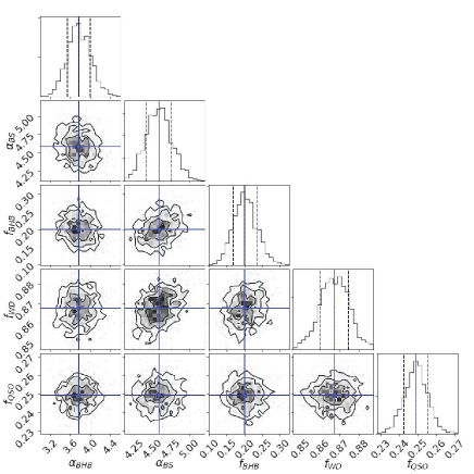
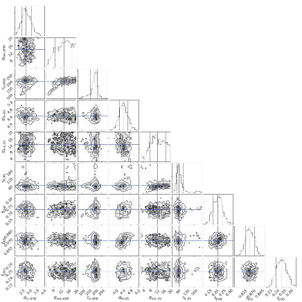
Figure 5: MCMC results for SSPL (left) and SBPL (right panel).

2.6 Maximum likelihood method for getting the radial density profile

We maximize the likelihood defined as

$$\ln\mathcal{L}=\sum_{i=1}^{N_{{\rm S}}} \Bigl{[}\Bigr{.} \tilde{f}_{{\rm BHB}}\tilde{\lambda}_{{\rm BHB}}(m_{i},l_{i},b_{i},griz_{i},seeing,\vec{\mu}_{\rm BHB})$$ (22)

$$+\tilde{f}_{{\rm BS}}\tilde{\lambda}_{{\rm BS}}(m_{i},l_{i},b_{i},griz_{i},seeing,\vec{\mu}_{\rm BS})$$

$$+\tilde{f}_{{\rm WD}}\tilde{\lambda}_{{\rm WD}}(m_{i},l_{i},b_{i},griz_{i},seeing)$$

$$+f_{{\rm QSO}}\tilde{\lambda}_{{\rm QSO}}(m_{i},l_{i},b_{i},griz_{i},seeing)$$

$$+ \tilde{\lambda}_{{\rm galaxy}}(m_{i},l_{i},b_{i},griz_{i},seeing)\Bigl{.}\Bigr{]}\ ,$$

where the subscript $i$ denotes each object and the summation is performed over all the sample. The fraction of each population ($\tilde{f}_{\rm WD}$, $\tilde{f}_{\rm BS}$, $\tilde{f}_{\rm BHB}$) is defined by the following equations with four free parameters ($f_{\rm BHB},f_{\rm BS},f_{\rm WD},f_{\rm QSO}$):

$$\tilde{f}_{{\rm WD}}=f_{{\rm WD}}(1-f_{{\rm QSO}})$$ (23)

$$\tilde{f}_{{\rm BS}}=(1-f_{{\rm BHB}})(1-f_{{\rm WD}})(1-f_{{\rm QSO}})$$ (24)

$$\tilde{f}_{{\rm BHB}}=f_{{\rm BHB}}(1-f_{{\rm WD}})(1-f_{{\rm QSO}})\ .$$ (25)

The function, $\tilde{\lambda}_{\rm Comp}$ with ${\rm Comp}=$ BHB, BS, WD, QSO and galaxy, denotes the probability of each population having $m$ ($g$-band apparent magnitude), Galactic coordiantes $(l,b)$, colors in $griz$, and the set of model parameters, $\vec{\mu}$, given for the halo density distributions of BHBs and BSs (such as a power-law index and broken radius) as introduced in the previous subsection. This is given as

$$\tilde{\lambda}_{{\rm Comp}}(m,l,b,griz,seeing,\vec{\mu})=$$

$$\int\Bigl{[}\Bigr{.}G(m,griz,M)\lambda_{{\rm Comp}}(m,l,b,griz,seeing,\vec{\mu})\Bigl{.}\Bigr{]}{\rm d}m\ {\rm d}(griz)\ {\rm d}M$$

$$\Bigl{/}\Bigr{.}\int\Bigl{[}\lambda_{{\rm Comp}}(m,l,b,griz,seeing,\vec{\mu})\Bigr{]}{\rm d}m\ {\rm d}(griz)\ {\rm d}l\ {\rm d}b$$ (26)

where the denominator is a normalization over the ranges of $griz$, $m_{g}$, $l$ and $b$ specified in Equation (1) and the numerator is to consider photometric error and deviation of absolute magnitude. $G(m,griz,M)$ is a fifth-dimensional normal distribution in $g-r$, $r-i$, $i-z$, apparent magnitude $m$ and absolute magnitude $M$, both in $g$-band in this work, i.e., $m_{g}$ and $M_{g}$. Here, for simplicity, we assume that the functional dependence on each variable is separable, so $G(m,griz,M)$ can be described as the multiplication of five one-dimensional normal distributions. Because of only small deviation in $M_{g}$ for BHB, their normal distribution can be approximated as a Dirac Delta so the integration for $M_{g}$ can be neglected.

For each population with the color distribution $p(griz\mid{\rm Comp})$ given in Equation (2) and with an estimated distance, $D$, we obtain the following equation.

• BHB

  $$\lambda_{{\rm BHB}}(m,l,b,griz,seeing,\vec{\mu}_{{\rm BHB}})=$$

  $$P_{{\rm star}}(m,seeing)p(griz\mid{\rm BHB})$$

  $$\rho_{{\rm halo}}(X,Y,Z\mid m,l,b,gr,\vec{\mu}_{{\rm BHB}})D^{3}(m,gr\mid{{\rm BHB}})\cos(b)$$ (27)

• BS

  $$\lambda_{{\rm BS}}(m,l,b,griz,seeing,\vec{\mu}_{{\rm BS}})=$$

  $$P_{{\rm star}}(m,seeing)p(griz\mid{\rm BS})$$

  $$\rho_{{\rm halo}}(X,Y,Z\mid m,l,b,gr,\vec{\mu}_{{\rm BS}})D^{3}(m,gr\mid{{\rm BS}})\cos(b)$$ (28)

• WD

  $$\lambda_{{\rm WD}}(m,l,b,griz,seeing)=$$

  $$P_{{\rm star}}(m,seeing)p(griz\mid{\rm WD})$$

  $$\rho_{{\rm disk}}(X,Y,Z\mid m,l,b,gr,\vec{\mu})D^{3}(m,gr\mid{{\rm WD}})\cos(b)$$ (29)

• QSO

  $$\lambda_{{\rm QSO}}(m,l,b,griz,seeing)=$$

  $$P_{{\rm star}}(m,seeing)p(griz\mid{\rm QSO})$$ (30)

• galaxy

  $$\lambda_{{\rm galaxy}}(m,l,b,griz,seeing)=$$

  $$(1-P_{{\rm star}}(m,seeing))p(griz\mid{\rm galaxy})$$ (31)

As described above, we estimate the best fit parameters using MCMC. We assume the prior distribution is uniform over a concerned range (see Table 2.5). The best-fit parameters have been estimated using the 50th percentile of the posterior distributions and the 16th and 84th percentiles have been used to estimate the 1-$\sigma$ uncertainties.

3 Results

In this section, we show our main results following the Bayesian method shown in Section 2 and compare with our previous work based on the different method for the selection of BHBs using the S16A data of HSC-SSP.

3.1 Best fit models

Table 2.5 shows the best fit parameters for the models of SSPL, SBPL, ASPL, ABPL and Einasto density profiles, respectively. The difference in the BIC values relative to that for the best fit case (ABPL) is also listed in the last column. Figures 5, 6 and 7 show the MCMC results for these models. We note that as given in Equation (1), these results correspond to the sample with the magnitude range of $18.5<g<23.5$, suggesting BHBs at about $r=36\sim 360$ kpc and BSs at about $r=16\sim 160$ kpc. The main properties of the results are summarized as follows.

• Both single power-law models of SSPL and ASPL reveal similar index values, i.e., BHBs are fit to $\alpha=3.7\sim 3.8$, whereas BSs show steeper density profiles of $\alpha=4.4\sim 4.6$.

• For BHBs, double power-law models (SBPL and ABPL) show slightly shallower profiles at $r<r_{\rm b}$ than the corresponding single power-law models (SSPL and ASPL) expressed as $\alpha_{\rm in}<\alpha$. For BSs, $\alpha_{\rm in}$ is basically the same as $\alpha$ within the 1$\sigma$ error.

• The non-spherical models of ASPL and ASBL suggest a prolate shape of $q=1.4\sim 1.8$.

• Both double power-law models of SBPL and ABPL show very steep index values of $\alpha_{\rm out}$ for both BHBs and BSs, suggesting outer boundaries in both populations.

• ABPL provides the lowest BIC, thus is most likely among the given models.

• The best-fit parameters for calculating the fractions of the populations, $f_{\rm BHB}$, $f_{\rm WD}$ and $f_{\rm QSO}$ are basically the same for different models. We then obtain the fraction of each population as $\tilde{f}_{\rm BHB}=0.0195-0.0218$, $\tilde{f}_{\rm BS}=0.0781-0.0815$ and $\tilde{f}_{\rm WD}=0.649-0.658$.

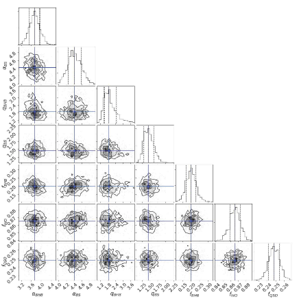
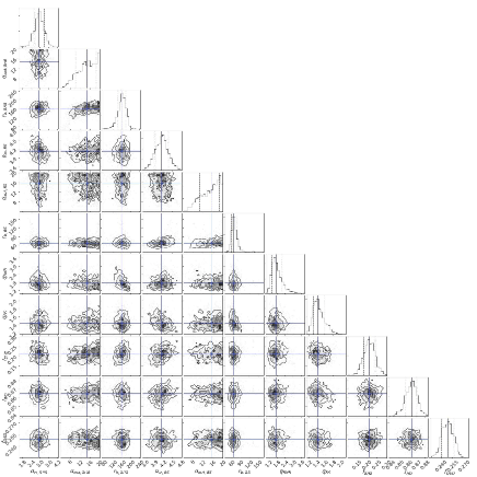
Figure 6: MCMC results for ASPL (left) and ABPL (right panel).

Figure 7: MCMC results for Einasto model.

We also consider the effects of some modification for the parameters of WDs, especially the scale height, $H_{2}$, for the thick-disk component, which is generally uncertain. We examine the case when the value of $H_{2}$ is modified from $0.9$ kpc to $2$ kpc for ABPL. It is found that the change in $\alpha_{\rm in}$ is confined to be about 10%. The changes in $\alpha_{\rm out}$ and $r_{b}$ are in the range of 13 to 21%, whereas the change in $q$ is up to 55%, although the halo shape remains to be prolate. Thus, we conclude that some minor modification for the parameters of WDs do not affect the general properties of the density profile for both BHBs and BSs.

3.2 Comparison with our previous work

In Fukushima et al. (2018), we reported our work based on the simple color cuts in $griz$ band for the selection of BHBs using the S16A data of HSC-SSP over $\sim 300$ deg² area. The main results in that paper for the case excluding the fields containing known substructures are roughly the same as those presented here, although there are some detailed differences. These previous results are summarized as $\alpha\simeq 3.5$ and $q\simeq 1.3$ for ASPL and $\alpha_{\rm in}\simeq 3.2$, $\alpha_{\rm out}\simeq 5.3$, $q\simeq 1.5$ and $r_{\rm eff}\simeq 210$ kpc for ABPL. This suggests that compared with these previous results, the current analysis gives somewhat steep $\alpha$ and large $q$ for ASPL, whereas $\alpha_{\rm out}$ is made quite steep for ABPL. This may be caused by the removal of more BS contamination from candidate BHBs in the outskirts of the halo based on the current Bayesian analysis than those made in our previous work, as well as the use of the HSC-SSP data over much larger survey areas.

To assess the above statement, we analyze the HSC-SSP data adopted in Fukushima et al. (2018) (with a magnitude limit of $g<22.5$) but using the method developed here. We obtain, for BHBs, $\alpha=4.12^{+0.83}_{-0.60}$ and $q=1.08^{+1.09}_{-0.55}$ for ASPL and $\alpha_{\rm in}=4.00^{+0.81}_{-0.89}$, $\alpha_{\rm out}=9.80^{+6.67}_{-4.99}$, $q=1.00^{+1.65}_{-0.51}$ and $r_{\rm eff}\sim 158.9^{+59.5}_{-61.9}$ kpc for ABPL. Thus, due to the removal of more BS contamination in the outskirts of the halo, the current new analysis leads somewhat steeper $\alpha$, although this change remains within the 1$\sigma$ error. In the current work using the S18A data, the axial ratio, $q$, is made larger than that using the S16A data. This may be due to the increase of the S18A sample at high Galactic latitudes, where the sensitively to the prolate shape of the stellar halo can be increased. In this manner, it is possible to understand the changes in the results from our previous work, and the current work is expected to provide more realistic model parameters having smaller errors.

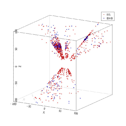
Figure 8: Three-dimensional distributions of BHBs (blue points) and BSs (red points) selected from those having high probabilities as BHBs [$p({\rm BHB}|x)>0.7$] and BSs [$p({\rm BS}|x)>0.7$], respectively, as defined in Equation (32). The left panel shows the box over $-200\leq x,y,z\leq 200$ kpc and the right panel shows the zoom-in view of the inner region over $-100\leq x,y,z\leq 100$ kpc.

3.3 Three-dimensional maps of BHBs and BSs

So far, we focus on the smooth parts of the stellar halo by excluding the fields, GAMA15H and XMM-LSS, which contain the known substructures including the Sgr stream. Given that the parameters $f_{\rm BHB}$, $f_{\rm WD}$ and $f_{\rm QSO}$ basically remain the same among different density models, it is possible to derive the probability that a given target is either of a BHB, BS, WD, QSO or galaxy. For instance, the probability of a BHB is given as

$$p({\rm BHB}|x)=\frac{p(x|{\rm BHB})f_{\rm BHB}}{\sum_{i=1}^{4}p(x|A_{i})\tilde{f}_{i}+p(x|{\rm galaxy})\frac{1-P_{\rm star}}{P_{\rm star}}}\ ,$$ (32)

where $x$ shows each sample and $i$ denotes a component (BHB, BS, WD and QSO).

Figure 8 shows the three-dimensional maps for the sample with $p({\rm BHB}|x)$ larger than 70% (blue points) and $p({\rm BS}|x)$ larger than 70% (red points) using all the survey fields. There is a substructure associated with the Sgr stream at around $(x,y,z)=(-20,10,40)$ kpc as seen for both BHBs and BSs. Sextans dSph is visible at $(x,y,z)=(40,60,60)$ kpc, and there appears an overdensity at $(x,y,z)=(0,-40,-50)$ kpc, which might be the tidal debris from the Large Magellanic Cloud (Diaz & Bekki, 2012).

Figure 9 shows the density distribution of BHBs (blue lines) and BSs (red lines), where the solid (dashed) lines correspond to these stars having probabilities larger than 80% (70%), namely $p({\rm BHB}|x)>0.8$ and $p({\rm BS}|x)>0.8$ ($p({\rm BHB}|x)>0.7$ and $p({\rm BS}|x)>0.7$). It follows that these high-probability sample stars show a signature of broken density profiles changed at $r\sim 160$ kpc for BHBs and $r\sim 70$ kpc for BSs, respectively, as suggested from the best-fit models in the previous subsection. We note that the actual density profiles are obtained over the integral of these probability distributions in our Bayesinan method.

Figure 9: The density distribution of BHBs (blue lines) and BSs (red lines), where the solid (dashed) lines correspond to these stars having probabilities larger than 80% (70%), namely $p({\rm BHB}|x)>0.8$ and $p({\rm BS}|x)>0.8$ ($p({\rm BHB}|x)>0.7$ and $p({\rm BS}|x)>0.7$).

Figure 10: Comparison of our best-fit models, the single power-law (blue solid line), broken power-law (blue dotted line), and the Einasto profile (blue dashed line), with other works using BHBs (Deason et al., 2011; Thomas et al., 2018) and RR Lyrae (Watkins et al., 2009; Cohen et al., 2017; Hernitschek et al., 2018).

4 Discussion

4.1 Comparison with other survey results

Many previous surveys for tracing the MW stellar halo have been made, as mentioned in Section 1, but except for the following recent works, the most of the other surveys are devoted to the halo regions at Galactocentric radii well below $r=100$ kpc. In this subsection, we compare our results with the other surveys for $r$ as large as 100 kpc, which are summarized in Figure 10.

Thomas et al. (2018) recently combined their CFIS survey made in deep $u$-band with $griz$-band data from Pan-STARRS 1 to select candidate BHBs. Their analysis revealed that a broken power-law model with an inner/outer slope of $4.24/3.21$ at a break radius of 41.4 kpc is the best fitting case out to $r\sim 220$ kpc. This outer slope is similar to the inner slope of $\simeq 2.92$ in our ABPL model at $r<r_{\rm b}\simeq 160$ kpc, thus giving an approximate agreement. In contrast, their model of a fixed axial ratio showed $q\simeq 0.86$, i.e., an oblate halo. However, their alternative model allowing a varying $q$ suggests a prolate halo in the outer halo, which is consistent with our results.

The surveys using RRLs at $r$ as large as 100 kpc tend to provide different density slopes (Watkins et al., 2009; Cohen et al., 2017; Hernitschek et al., 2018). These works show $\alpha=4.0\sim 4.5$ at $r>25$ kpc, which is systematically steeper than the slopes obtained here for BHBs, but consistent with those for BSs located at similar radii to RRLs ($\alpha\simeq 4.50$ for ASPL, $\alpha_{\rm out}\simeq 4.22$ for ABPL). This implies that the difference in the value of the density slope for BHBs from that for RRLs is due to the difference in the range of Galactocentric radii for the adopted sample. Another possible reason for the different slopes may be due to the intrinsically different radial distribution for a different stellar sample, depending on the formation history of a stellar halo associated with merging/accretion of progenitor dwarf galaxies as discussed in the next subsection.

Our current work suggests that the density slope of the MW halo is somewhat shallower at $r>100$ kpc as probed by BHBs than the slope at radii near and below $\sim 100$ kpc. Also, the very steep slope at radii above $\simeq 160$ kpc for BHBs may suggest a sharp outer edge of the stellar halo. On the other hand, a steeper $\alpha$ and smaller break radius ($r_{\rm b}\simeq 70$ kpc) for BSs may be due to the intrinsically more centrally concentrated spatial distribution of BSs than BHBs in the MW halo. This may be caused by the more centrally distributed BSs in progenitor dwarf galaxies (e.g., Wang et al. (2018)): in the course of merging/accretion of dwarf galaxies, these denser, central parts can fall into the more central parts of the MW halo due to the effects of dynamical friction, so that the debris after the destruction of dwarf galaxies reflect the original internal distribution inside dwarf galaxies.

4.2 Possible constraints on the past accretion history

To infer what constraints from the current analysis of BHBs can be made on the past accretion history of the MW halo, we compare our results with the suite of hydrodynamical simulations for galaxy formation by Rodriguez-Gomez et al. (2016) using the Illustris Project (Genel et al., 2014; Vogelsberger et al., 2014a, b). Rodriguez-Gomez et al. (2016) investigated the formation of galaxies over a wide range of stellar masses, $M_{\ast}=10^{9}-10^{12}M_{\odot}$, and obtained the relative contribution of the so-called in situ. halo (main progeitor halo) with respect to the ex situ. halo (accreted stellar system from outside) component. It is found that these halo components are spatially segregated, with in situ. halo dominating the innermost regions of the halo space, and ex situ. halo being deposited at larger Galactocentric distances in order of decreasing merger mass ratio. These properties are well summarized in their Figure 10: the in situ. component shows a steep density profile below the transition radius, whereas the ex situ. component beyond this radius provides a shallow slope having an outer boundary. This theoretical prediction may well reproduce the change of the halo density profile mentioned in the previous subsection, namely the steep profile in the inner halo probed by RRLs, which were possibly formed in situ., and the shallow profile in the outer halo reported here using BHBs, which were originated from the ex situ. component.

5 Conclusions

Using the HSC-SSP Wide layer data obtained until 2018 April (S18A), which covers $\sim 550$ deg² area, we have selected candidate BHB stars based on the $(g,r,i,z)$ photometry, where $z$-band brightness can be used to probe a surface gravity of a BHB star against other A-type stars. In contrast to our previous work reported in Fukushima et al. (2018), where the simple color cuts were adopted for the selection of BHBs, we have developed an extensive Bayesian method to minimize the effects of non-BHB contamination as much as possible. In this analysis, the distributions of the template BHBs and non-BHB populations are represented as a mixture of multiple Gaussians in the color-color diagrams defined in $griz$ band. This method is especially effective for removing BS contamination in a statistically significant manner.

Applying to the sample with $18.5<g<23.5$, which, for candidate BHBs, correspond to the positions of Galactocentric radii at $r=36\sim 360$ kpc, we have obtained the density slopes of BHBs for a single power-law model as $\alpha=3.74^{+0.21}_{-0.22}$ and for a broken power-law model as $\alpha_{\rm in}=2.92^{+0.33}_{-0.33}$ and $\alpha_{\rm out}=15.0^{+3.7}_{-4.5}$ divided at a radius of $r_{\rm b}=160^{+18}_{-19}$ kpc. The latter power-law model appears most likely according to BIC. For the models allowing a non-spherical halo shape, an axial ratio of $q=1.72^{+0.44}_{-0.28}$ corresponding to a prolate shape is the most likely case. It is also suggested from a very steep $\alpha_{\rm out}$ that the MW stellar halo may have a sharp boundary at $r=r_{\rm b}\simeq 160$ kpc, although this needs to be assessed using the further survey data.

The density slope obtained in this work is basically in agreement with that from the recent CFIS survey for BHBs (Thomas et al., 2018). However, it is systematically shallower than the slope derived from RRL stars at $r$ below $\sim 100$ kpc (Cohen et al., 2017; Hernitschek et al., 2018). This may be simply due to the different radial range of each sample, $r<100$ kpc for RRLs and $50<r<360$ kpc for BHBs, or RRLs may have an intrinsically more centrally concentrated distribution than BHBs. However, before concluding so, we require much larger data for BHBs obtained by the completion of the HSC-SSP survey with a goal of $\sim 1,400$ deg². Also, to interpret such observational results in the form of the past merging history, more extensive numerical simulations for the formation of stellar halos will be important, where not only accretion/merging of satellites from outside but also the in situ. formation of halo stars are properly taken into account.

This work is supported in part by JSPS Grant-in-Aid for Scientific Research (B) (No. 25287062) and MEXT Grant-in-Aid for Scientific Research (No. 16H01086, 17H01101 and 18H04334 for MC, No. 18H04359 and No. 18J00277 for KH). TM is supported by Grant-in-Aid for JSPS Fellows (No. 18J11326).

The Hyper Suprime-Cam (HSC) collaboration includes the astronomical communities of Japan and Taiwan, and Princeton University. The HSC instrumentation and software were developed by the National Astronomical Observatory of Japan (NAOJ), the Kavli Institute for the Physics and Mathematics of the Universe (Kavli IPMU), the University of Tokyo, the High Energy Accelerator Research Organization (KEK), the Academia Sinica Institute for Astronomy and Astrophysics in Taiwan (ASIAA), and Princeton University. Funding was contributed by the FIRST program from Japanese Cabinet Office, the Ministry of Education, Culture, Sports, Science and Technology (MEXT), the Japan Society for the Promotion of Science (JSPS), Japan Science and Technology Agency (JST), the Toray Science Foundation, NAOJ, Kavli IPMU, KEK, ASIAA, and Princeton University. This paper makes use of software developed for the Large Synoptic Survey Telescope. We thank the LSST Project for making their code freely available. The Pan-STARRS1 (PS1) Surveys have been made possible through contributions of the Institute for Astronomy, the University of Hawaii, the Pan-STARRS Project Office, the Max-Planck Society and its participating institutes, the Max Planck Institute for Astronomy and the Max Planck Institute for Extraterrestrial Physics, The Johns Hopkins University, Durham University, the University of Edinburgh, Queen’s University Belfast, the Harvard-Smithsonian Center for Astrophysics, the Las Cumbres Observatory Global Telescope Network Incorporated, the National Central University of Taiwan, the Space Telescope Science Institute, the National Aeronautics and Space Administration under Grant No. NNX08AR22G issued through the Planetary Science Division of the NASA Science Mission Directorate, the National Science Foundation under Grant No.AST-1238877, the University of Maryland, and Eotvos Lorand University (ELTE).

References

- Abazajian et al. (2004) Abazajian, K., Adelman-McCarthy, J. K., Agüeros, M. A., et al. 2004, AJ, 128, 502
- Aihara et al. (2018a) Aihara, H., Arimoto, N., Bickerton, S., et al. 2018a, PASJ, 70, S4 (arXiv:1704.05858)
- Aihara et al. (2018b) Aihara, H., Armstrong, R., Bickerton, S., et al. 2018b, PASJ, 70, S8 (arXiv:1702.08449)
- Axelrod et al. (2010) Axelrod, T., Kantor, J., Lupton, R. H., & Pierfederici, F. 2010, in Proc. SPIE, Vol. 7740, Software and Cyberinfrastructure for Astronomy, 774015
- Belokurov et al. (2006) Belokurov, V., Zucker, D. B., Evans, N. W., et al. 2006, ApJ, 647, L11
- Bland-Hawthorn & Freeman (2014) Bland-Hawthorn, J., & Freeman, K., 2014, The Origin of the Galaxy and Local Group, Saas-Fee Advanced Course, Vol. 37 (Springer)
- Bosch et al. (2018) Bosch, J., Armstrong, R., Bickerton, S., et al. 2018, PASJ, 70, S5
- Bovy et al. (2011) Bovy J., Hogg D. W., Roweis S. T., 2011, Annals of Applied Statistics, 5, 1657
- Bullock & Johnston (2005) Bullock, J. S. & Johnston, K. V. 2005, ApJ, 635, 931
- Chen et al. (2001) Chen, B., Stoughton, C., Smith, J. A., et al. 2001, ApJ, 553, 184
- Cohen et al. (2015) Cohen, J. G., Sesar, B., Banholzer, S., the PTF Collaboration, 2015, IAU General Assembly, 22, 2255152
- Cohen et al. (2017) Cohen, J. G., Sesar, B., Banholzer, S. et al. 2017, ApJ, 849, 150
- Cooper et al. (2010) Cooper, A. P. et al., 2010, MNRAS, 406. 744
- Deason et al. (2011) Deason, A. J., Belokurov, V., & Evans, N. W. 2011, MNRAS, 416, 2903
- Deason et al. (2014) Deason, A. J., Belokurov, V., Koposov S. E., Rockosi C. M. 2014, ApJ, 787, 30
- Deason et al. (2018a) Deason, A. J., Belokurov, V., Koposov S. E. 2018a, ApJ, 852, 118
- Deason et al. (2018b) Deason, A. J., Belokurov, V., Koposov S. E., & Lancaster, L. 2018b, arXiv:1805.10288
- Diaz & Bekki (2012) Diaz, J., & Bekki, K. 2012, ApJ, 750, 36
- Einasto (1965) Einasto, J. 1965, Trudy Inst. Astroz. Alma-Ata, 5, 87
- Feltzing & Chiba (2013) Feltzing, S., & Chiba, M. 2013, New Astronomy Reviews, 57, 80
- Foreman-Mackey et al. (2013) Foreman-Mackey D., Hogg D. W., Lang D., Goodman J., 2013, PASP, 125, 306
- Fukushima et al. (2018) Fukushima, T., Chiba, M., et al. 2018, PASJ, 70, 69
- Furusawa et al. (2018) Furusawa, H., et al. 2018, PASJ, 70, S3
- Genel et al. (2014) Genel, S. et al. 2014, MNRAS, 445, 175
- Goodman & Weare (2010) Goodman J., Weare J., 2010, Comm. App. Math. Comp. Sci., 5, 65
- Graham et al. (2006) Graham, A. W., Merritt, D., Moore, B., et al. 2006, AJ, 132, 2701
- Grand et al. (2017) Grand, R. J. J., et al. 2017, MNRAS, 467, 179
- Gunn & Stryker (1983) Gunn, J. E., & Stryker, L. L., 1983, ApJS, 52, 121
- Helmi & White (1999) Helmi, A. & White, S. D. M., 1999, MNRAS, 307, 495
- Helmi (2008) Helmi, A. 2008, A&ARV, 15, 145
- Hernitschek et al. (2018) Hernitschek, N., Cohe, J. G., Rix, H.-W., et al., 2018, ApJ, 859, 31
- Holoien et al. (2017) Holoien T. W.-S., Marshall P. J., Wechsler R. H., 2017, AJ, 153, 249
- Homma et al. (2016) Homma, D., Chiba, M., Okamoto, S., et al. 2016, ApJ, 832, 21
- Ibata et al. (1995) Ibata, R. A., Gilmore, G., Irwin, M. J. 1995, MNRAS, 277, 781
- Ivezić et al. (2008) Ivezić, Z., Axelrod, T., Brandt, W. N., et al. 2008, AJ, 176, 1
- Ivezić, Beers & Juric (2012) Ivezić, Z., Beers, T. C., & Jurić, M. 2012, ARAA, 50, 251
- Jurić et al. (2008) Jurić, M., Ivezić, Z., Brooks, A., et al. 2008, ApJ, 673, 864
- Jurić et al. (2017) Jurić, M., Kantor, J., Lim, K.-T., et al. 2017, ASPC, 512, 279
- Kawanomoto et al. (2018) Kawanomoto, S. et al. 2018, PASJ, 70, 66
- Keller et al. (2008) Keller, S. C., Murphy, S., Prior, S., Da Costa, G., & Schmidt, B. 2008, ApJ, 678, 851
- Kepler et al. (2015) Kepler, S. O., Pelisoli, I., Koester, D., et al. 2015, MNRAS, 446, 4078
- Kepler et al. (2016) Kepler, S. O., Pelisoli, I., Koester, D., et al. 2016, MNRAS, 455, 3413
- Kleinman et al. (2013) Kleinman, S. J., Kepler, S. O., Koester, D., et al. 2013, ApJS, 204, 5
- Komiyama et al. (2018) Komiyama, Y., et al. 2018, PASJ, 70, S2
- Lee et al. (2008) Lee, Y. S., Beers, T. C., Sivarani, T., et al. 2008, AJ, 136, 2022.
- Lenz et al. (1998) Lenz, D. D., Newberg, J., Rosner, R., et al. 1998, ApJS, 119, 121
- Magnier et al. (2013) Magnier, E. A., Schlafly, E., Finkbeiner, D., et al. 2013, ApJS, 205, 20
- Miyazaki et al. (2018) Miyazaki, S., Komiyama, Y., Kawanomoto, S. et al. 2018, PASJ, 70, S1
- Monachesi et al. (2018) Monachesi, A. et al. 2018, arXiv:1804.07798
- Newberg & Yanny (2005) Newberg, H. J., & Yanny, B. 2005, JPhCS, 47, 195
- Pâris et al. (2018) Pâris I. et al. 2018, A&A, 613, A51
- Pillepich et al. (2014) Pillepich, A., Vogelsberger, M., Deason, A., et al. 2014, MNRAS, 244, 237
- Rodriguez-Gomez et al. (2016) Rodriguez-Gomez, V., Pillepich, A., Sales, L. V. et al. 2016, MNRAS, 458, 2371
- Schlafly & Finkbeiner (2011) Schlafly, E. F., & Finkbeiner, D. P. 2011, ApJ, 737, 103
- Schlafly et al. (2012) Schlafly, E. F., Finkbeiner, D. P., Jurić, M., et al. 2012, ApJ, 756, 158
- Searle & Zinn (1978) Searle, L., & Zinn, R. 1978, ApJ, 225, 357
- Sesar et al. (2011) Sesar, B, Jurić, M., & Ivezić, Z. 2011, ApJ, 731, 4
- Sirko et al. (2004) Sirko, E., Goodman, J., Knapp, G. R., et al. 2004, AJ, 127, 899
- Slater et al. (2016) Slater, C. T., Nidever, D. L., Munn, J. A., Bell, E. F., & Majewski, S. R. 2016, ApJ, 832, 206
- Sluis & Arnold (1998) Sluis, A. P. N., & Arnold, R. A. 1998, MNRAS, 297, 732
- Thomas et al. (2018) Thomas, G. A., McConnachie, A. W., Ibata, R. A., et al. 2018, MNRAS, 481, 5223
- Tonry et al. (2012) Tonry, J. L., Stubbs, C. W., Lykke, K. R., et al. 2012, ApJ, 750, 99
- Vickers et al. (2012) Vickers, J. J., Grebel, E. K., & Huxor, A. P. 2012, AJ, 143, 86
- Vivas et al. (2016) Vivas, A. K., Zinn, R., Farmer, J., et al. 2016, ApJ, in press (arXiv:1608.08981)
- Vogelsberger et al. (2014a) Vogelsberger, M. et al. 2014a, Nature, 509, 177
- Vogelsberger et al. (2014b) Vogelsberger, M. et al. 2014b, MNRAS, 444, 1518
- Wang et al. (2018) Wang, M.-Y. et al. 2018, preprint (arXiv: 1809.07801)
- Watkins et al. (2009) Watkins, L. L. et al. 2009, MNRAS, 398, 1757
- Xu et al. (2018) Xu, Y., Liu, C., Xue, X.-X., et al. 2018, MNRAS, 473, 1244
- Xue et al. (2011) Xue, X.-X., Rix, H.-W., Yanny, B., et al. 2011, ApJ, 738, 79
- Yanny et al. (2000) Yanny, B., Newberf, H. J., Kent, S., et al. 2000, ApJ, 540,825