Three two-component fermions with contact interactions: correct formulation and energy spectrum

Abstract

Properties of two identical particles of mass $m$ and a distinct particle of mass $m_{1}$ in the universal low-energy limit of zero-range two-body interaction are studied in different sectors of total angular momentum $L$ and parity $P$. For the unambiguous formulation of the problem in the interval $\mu_{r}(L^{P})<m/m_{1}\leq\mu_{c}(L^{P})$ ($\mu_{r}(1^{-})\approx 8.619$ and $\mu_{c}(1^{-})\approx 13.607$, $\mu_{r}(2^{+})\approx 32.948$ and $\mu_{c}(2^{+})\approx 38.630$, etc.) in each $L^{P}$ sector an additional parameter $b$ determining the wave function near the triple-collision point is introduced; thus, a one-parameter family of self-adjoint Hamiltonians is defined. Within the framework of this formulation, dependence of the bound-state energies on $m/m_{1}$ and $b$ in the sector of angular momentum and parity $L^{P}$ is calculated for $L\leq 5$ and analysed with the aid of a simple model. A number of the bound states for each $L^{P}$ sector is analysed and presented in the form of “phase diagrams” in the plane of two parameters $m/m_{1}$ and $b$.

I Introduction.

Motivation

In the present time, properties of multi-component ultra-cold quantum gases are on demand experimentally Jag et al. (2016) and theoretically Ospelkaus et al. (2006); Fratini and Pieri (2012); Iskin and Sá de Melo (2006); Levinsen et al. (2009); Mathy et al. (2011); Alzetto et al. (2012); Jag et al. (2014). Different aspects of few-body dynamics in two-species mixtures has attracted much attention.

At low energy the dependence on potential form is disappear, therefore, zero-range model (ZRM) is a good approximation for such systems. There are many advantages of using ZRM. First at all, the only parameter of the interaction, namely, the two-body scattering length $a$, can be taken as a scale, (or scale $a\to\infty$) that lead to parameterless description of the two-body problem. Then, for three- and more-body problem, one expects the few-parameter or even the parameterless description of the essential dynamical features of such systems. The usage of ZRM allows one to obtain simple and even exact solutions or reduce the calculation problems with increasing a number of particle in system, obtain the predictions of new effects and make some proposals for the future study most interesting one theoretically or experimentally. Moreover, model provides full description within limited class and allows to calculate universal constants (such as energies of the bound states, scattering characteristics, critical parameters of the system and so one).

Problem

The present paper is devoted to one of the principal issue, the study of few two-species particles, namely, two identical particles (bosons or fermions) of mass $m$ interacting with a distinct particle of mass $m_{1}$ in the s-wave. In the universal low-energy limit, the interaction between two identical fermions is forbidden in the s-wave and is strongly suppressed between two heavy bosons in the states of $L>0$, so that explain why one neglect the interaction of identical particles. To obtain the universal (independent of the particular form of the interaction) description of the system, the two-body interaction is taken in the framework of the ZRM. Then, by using proper units, one could expect formally the one-parameter $m/m_{1}$-dependence of the few-body properties.

Former results

One of the main features of this three-body problem (namely, two identical fermions and a distinct particle) is a principal role of the states with unit total angular momentum and negative parity $L^{P}=1^{-}$ in the low-energy processes Kartavtsev and Malykh (2007a); Petrov (2003); Kartavtsev and Malykh (2016). As it was already pointed out, there are three regions of the mass ratios, $m/m_{1}<\mu_{r}$, $\mu_{r}<m/m_{1}\leq\mu_{c}$, and $m/m_{1}>\mu_{c}$, where $\mu_{c}\approx 13.607$, $\mu_{r}\approx 8.619$. In the first region, formal three-body Hamiltonian is self-consistent and there is zero and one bound state for $m/m_{1}<8.17$ and $8.17\leq m/m_{1}\leq\mu_{r}$, respectively Kartavtsev and Malykh (2007a). For other two regions, the formal construction of the Hamiltonian does not obviously provide an unambiguous definition of the three-body problem; in particular, one is required an additional parameter, which determines the wave function in the vicinity of the triple-collision point (TCP). The third region, $m/m_{1}>\mu_{c}$, is well-known Efimov one with an infinite number of the bound states Efimov (1973). The necessity of correct formulation of the three-body problem for the second region, $\mu_{r}<m/m_{1}\leq\mu_{c}$, was indicated in both physical Nishida et al. (2008); Safavi-Naini et al. (2013); Kartavtsev and Malykh (2014) and mathematical Minlos (2011a, 2012, 2014a, 2014b); Correggi et al. (2012, 2015a, 2015b) papers. As was done in Kartavtsev and Malykh (2016), a one-parameter family of self-adjoint Hamiltonians was defined by introducing an additional three-body parameter $b$, which has a meaning of three-body scattering length. As a result, the properties of the energy spectrum of three-body system with two identical fermions for $L^{P}=1^{-}$ sector is studied in dependence on the mass-ratio and parameter $b$, whereas the scattering properties was investigated in dependence on the mass-ratio for particular case of the three-body parameter $b=0$ Kartavtsev and Malykh (2007a); Petrov (2003).

Despite this, one have to extend the problem for the arbitrary $L^{P}$ sector of angular momentum $L$ and parity $P$ and to consider simultaneously the system with two identical bosons and a distinct particle. As it is already known, the bound states can be found only for odd $L$ and $P$ if identical particles are fermions and for even $L$ and $P$ if identical particles are bosons. Such systems will be considered below. As in $L^{P}=1^{-}$ sector, there are three regions of the mass ratios, $m/m_{1}\leq\mu_{r}(L^{P})$, $\mu_{r}(L^{P})<m/m_{1}\leq\mu_{c}(L^{P})$, and $m/m_{1}>\mu_{c}(L^{P})$, where values $\mu_{r}(L^{P})$ and $\mu_{c}(L^{P})$ are presented in Table 1. As follows from the analyses of the wave function in the vicinity of the TCP Petrov (2003); Nishida et al. (2008); Kartavtsev and Malykh (2014, 2016), the problem of the correct formulation exists and has been done for mass ratio values $\mu_{r}(L^{P})<m/m_{1}\leq\mu_{c}(L^{P})$. Until now, in a number of reliable investigations of three two-component particles (for $m/m_{1}\leq\mu_{c}(L^{P})$) Petrov (2003); Kartavtsev and Malykh (2007a, b); Endo et al. (2011); Helfrich and Hammer (2011) it was explicitly or implicitly assumed the fastest decrease of the wave function near the TCP, i.e., that correspond to $b=0$.

Goal

The main aim of this paper is to formulate the three-body problem in the mass-ratio region $\mu_{r}(L^{P})<m/m_{1}\leq\mu_{c}(L^{P})$ in an arbitrary $L^{P}$ sector (more exactly, for odd $L$ and $P$ if identical particles are fermions and for even $L$ and $P$ if identical particles are bosons) by introducing the additional parameter $b$ as it was done in Kartavtsev and Malykh (2016) for $L^{P}=1^{-}$ sector. In such way, one has to construct a family of self-adjoint Hamiltonians, which depends on one parameter $b$, describing the solution behaviour at the TCP. Then one need to calculate the energy spectrum in an arbitrary $L^{P}$ sector as a function of $m/m_{1}$ and a set of three-body parameters $\{b_{L}\}$.

Consider a three-body problem for particle $1$ of mass $m_{1}$ interacting with two identical particles $2$ and $3$ of mass $m_{2}=m_{3}=m$ via the zero-range potential, which is completely described by the scattering length $a$. In the center-of-mass frame, define the scaled Jacobi variables as ${\mathbf{x}}=\displaystyle\sqrt{2\mu}\left({\mathbf{r}}_{2}-{\mathbf{r}}_{1}\right)$ and ${\mathbf{y}}=\displaystyle\sqrt{2\tilde{\mu}}\left({\mathbf{r}}_{3}-\frac{m_{1}{\mathbf{r}}_{1}+m{\mathbf{r}}_{2}}{m_{1}+m}\right)$, where ${\mathbf{r}}_{i}$ are the position vectors and $\mu=\displaystyle\frac{mm_{1}}{m+m_{1}}$, $\tilde{\mu}=\displaystyle\frac{m(m+m_{1})}{m_{1}+2m}$ are the reduced masses. Throughout the paper units are chosen to provide $\hbar=|a|=2m/(1+m/m_{1})=1$ that gives unit binding energies of the two-body subsystems, $\varepsilon_{12}=\varepsilon_{13}=1$.

The three-body wave function is a solution of

$$\left[\Delta_{{\bf x}}+\Delta_{{\bf y}}+E\right]\Psi({\bf x},{\bf y})=0\ ,$$ (1)

and

$$\lim_{r\rightarrow 0}\frac{\partial\ln(r\Psi)}{\partial r}=-\operatorname{sgn}(a)\ ,$$ (2)

where the boundary conditions (2) with $r=|{\mathbf{r}}_{1}-{\mathbf{r}}_{i}|$ and $i=2,3$ represent the zero-range potential in both pairs of distinct particles. The Hamiltonian is formally defined by Eqs. (1), (2) and depends only on the mass ratio $m/m_{1}$. The wave function is symmetrical or anti-symmetrical under permutation of identical particles ${\mathrm{P}}_{23}$, satisfying the condition

$${\mathrm{P}}_{23}\Psi({\mathbf{x}},{\mathbf{y}})=S\ \Psi({\mathbf{x}},{\mathbf{y}}),$$ (3)

where $S=-1$ ($S=1$) indicates that particles $2$ and $3$ are fermions (bosons). Total angular momentum $L$, its projection $M$, parity $P$, and index of permutational symmetry $S$ are conserved quantum numbers, which will be used to label the solutions. Only the states of parity $P=(-)^{L}$, i. e., for $P$ and $L$ odd or even simultaneously, need to be considered, as the states of opposite parity correspond to three non-interacting particles for the zero-range potential. As the system’s properties are independent of $M$, a complete description of the three-body problem, e. g., energy levels, will be given by the formal one-parameter Hamiltonian depending on $m/m_{1}$ in different $\{S,L\}$ sectors.

I.1 Hyper-radial equations

Let us define a hyper-radius $\rho$ and hyper-angular variables $\{\alpha,\hat{\mathbf{x}},\hat{\mathbf{y}}\}$ by $x=\rho\cos\alpha$, $y=\rho\sin\alpha$, $\hat{\mathbf{x}}={\mathbf{x}}/x$, and $\hat{\mathbf{y}}={\mathbf{y}}/y$. To produce a convenient basis for expansion of the total wave function defined by Eqs. (1), (2), introduce an auxiliary eigenvalue problem on a hyper-sphere (for fixed parameter $\rho$) Macek (1968),

$$\left[\frac{1}{\sin^{2}2\alpha}\left(\sin^{2}2\alpha\frac{\partial}{\partial\alpha}\right)+\frac{1}{\sin^{2}\alpha}\Delta_{\hat{\mathbf{x}}}+\frac{1}{\cos^{2}\alpha}\Delta_{\hat{\mathbf{y}}}+\gamma^{2}(\rho)-4\right]\Phi(\alpha,\hat{\mathbf{x}},\hat{\mathbf{y}};\rho)=0\ ,$$ (4)

$$\lim_{\alpha\rightarrow\pi/2}\frac{\partial\log\left[(\alpha-\pi/2)\Phi\right]}{\partial\alpha}=\rho\,\operatorname{sgn}(a)\ ,$$ (5)

along with the symmetry condition (3) for $\Phi(\alpha,\hat{\mathbf{x}},\hat{\mathbf{y}};\rho)$. Its square-integrable solutions form an infinite set of functions $\Phi_{n}(\alpha,\hat{\mathbf{x}},\hat{\mathbf{y}};\rho)$ enumerated by index $1\leq n<\infty$ in ascending order of the corresponding eigenvalues $\gamma^{2}_{n}(\rho)$.

Besides fermionic (bosonic) symmetry, the functions $\Phi(\alpha,\hat{\mathbf{x}},\hat{\mathbf{y}};\rho)$ inherit all the conserved quantum numbers of the total wave function. Solution of (4), (5) satisfying (3) will be found in the form Kartavtsev and Malykh (2007a, b, 2016)

$$\Phi(\alpha,\hat{\mathbf{x}},\hat{\mathbf{y}};\rho)=(1+S\ {\mathrm{P}}_{23})\frac{\varphi^{L}(\alpha)}{\sin 2\alpha}Y_{LM}(\hat{\mathbf{y}})\,,$$ (6)

where $Y_{LM}(\hat{\mathbf{y}})$ is the spherical function. The action of ${\mathrm{P}}_{23}$ in terms of the Jacobi variables is given by

$${\mathrm{P}}_{23}\left(\begin{array}[]{c}{\mathbf{x}}\\ {\mathbf{y}}\end{array}\right)=\left(\begin{array}[]{cr}-\sin\omega&\cos\omega\\ -\cos\omega&-\sin\omega\end{array}\right)\left(\begin{array}[]{c}{\mathbf{x}}\\ {\mathbf{y}}\end{array}\right)\ ,$$ (7)

where $\omega$ is related to the mass ratio by $\sin\omega=1/(1+m_{1}/m)$. To impose the boundary condition (5), one takes the limit $x\to 0$ in Eq. (7) and finds ${\mathrm{P}}_{23}\alpha\to\omega$ and ${\mathrm{P}}_{23}Y_{LM}(\hat{\mathbf{y}})\to(-1)^{L}Y_{LM}(\hat{\mathbf{y}})$ in the limit $\alpha\to\pi/2$. As a result, one comes to the eigenvalue problem

$$\left[\frac{d^{2}}{d\alpha^{2}}-\frac{L(L+1)}{\sin^{2}\alpha}+\gamma^{2}\right]\varphi^{L}(\alpha)=0\ ,$$ (8)

and

$$\varphi^{L}(0)=0\ ,$$ (9a)

$$\lim_{\alpha\rightarrow\pi/2}\left(\frac{d}{d\alpha}-\rho\,\operatorname{sgn}(a)\right)\varphi^{L}(\alpha)=\frac{2S(-)^{L}}{\sin 2\omega}\varphi^{L}(\omega)\,.$$ (9b)

Solution of (8) and (9a) is discussed in Appendix A. The boundary condition (9b), along with (36), (39), and (40), gives the transcendental equation

$$\rho\operatorname{sgn}(a)\Gamma\left(\frac{L+1+\gamma}{2}\right)\Gamma\left(\frac{L+1-\gamma}{2}\right) =$$

$$2\Gamma\left(\frac{L+\gamma}{2}+1\right)\Gamma\left(\frac{L-\gamma}{2}+1\right)-S \frac{2^{1-L}\pi(\sin\omega)^{L}}{\sin\gamma\pi\cos\omega}\frac{d^{L}}{d(\cos\omega)^{L}}\frac{\sin\gamma\omega}{\sin\omega}$$ (10)

determining $\rho\operatorname{sgn}(a)$ as an even single-valued function of $\gamma$. The inverse function is multi-valued, which different branches form a set of eigenvalues $\gamma^{2}_{n}(\rho)$ and, accordingly, a set of $\varphi_{n}(\rho)$ and $\Phi_{n}(\alpha,\hat{\mathbf{x}},\hat{\mathbf{y}};\rho)$. In particular, the transcendental equation takes the well-known form for $L=0$,

$$\rho\operatorname{sgn}(a)\sin\gamma\frac{\pi}{2}=\gamma\cos\gamma\frac{\pi}{2}-2S\frac{\sin\gamma\omega}{\sin 2\omega}\ .$$ (11)

Expansion of the total wave function Macek (1968),

$$\Psi=\rho^{-5/2}\sum_{n=1}^{\infty}f_{n}(\rho)\Phi_{n}(\alpha,\hat{\mathbf{x}},\hat{\mathbf{y}};\rho)\,,$$ (12)

leads to a system of hyper-radial equations (HREs) for the channel functions $f_{n}(\rho)$,

$$\left[\frac{d^{2}}{d\rho^{2}}-V_{n}(\rho)+E\right]f_{n}(\rho)-\sum_{m\neq n}^{\infty}\left[P_{nm}(\rho)-Q_{nm}(\rho)\frac{d}{d\rho}-\frac{d}{d\rho}Q_{nm}(\rho)\right]f_{m}(\rho)=0\,.$$ (13)

Here the diagonal terms

$$V_{n}(\rho)=\frac{\gamma_{n}^{2}(\rho)-1/4}{\rho^{2}}+P_{nn}(\rho)$$ (14)

play a role of the effective channel potentials, the coupling terms are defined as $Q_{nm}(\rho)=\displaystyle\left\langle\Phi_{n}\biggm{|}\frac{\partial\Phi_{m}}{\partial\rho}\right\rangle$ and $P_{nm}(\rho)=\displaystyle\left\langle\frac{\partial\Phi_{n}}{\partial\rho}\biggm{|}\frac{\partial\Phi_{m}}{\partial\rho}\right\rangle$, and the notation $\langle\cdot|\cdot\rangle$ means integration over the invariant volume on a hypersphere $\sin^{2}{2\alpha}\,d\alpha\,d\hat{\mathbf{x}}d\hat{\mathbf{y}}$. For the zero-range interaction, suitable analytical expressions via $\gamma^{2}_{n}(\rho)$ and their derivatives are derived Kartavtsev (1999); Kartavtsev and Malykh (2006, 2007a),

$$\hskip-22.76228ptQ_{nm}(\rho)=\left(\gamma_{n}^{2}-\gamma_{m}^{2}\right)^{-1}\sqrt{\frac{d\gamma_{n}^{2}}{d\rho}\frac{d\gamma_{m}^{2}}{d\rho}}\,,$$ (15)

$$\hskip-22.76228ptP_{nm}(\rho)=Q_{nm}(\rho)\left[\frac{1}{\left(\gamma_{m}^{2}-\gamma_{n}^{2}\right)}\frac{d}{d\rho}\left(\gamma_{n}^{2}+\gamma_{m}^{2}\right)+\frac{1}{2}\frac{d^{2}\gamma_{n}^{2}}{d\rho^{2}}\left(\frac{d\gamma_{n}^{2}}{d\rho}\right)^{-1}-\frac{1}{2}\frac{d^{2}\gamma_{m}^{2}}{d\rho^{2}}\left(\frac{d\gamma_{m}^{2}}{d\rho}\right)^{-1}\right],$$ (16)

$$\hskip-22.76228ptP_{nn}(\rho)=-\frac{1}{6}\frac{d^{3}\gamma_{n}^{2}}{d\rho^{3}}\left(\frac{d\gamma_{n}^{2}}{d\rho}\right)^{-1}+\frac{1}{4}\left(\frac{d^{2}\gamma_{n}^{2}}{d\rho^{2}}\right)^{2}\left(\frac{d\gamma_{n}^{2}}{d\rho}\right)^{-2}\ .$$ (17)

For correct definition of the three-body problem and solution of a system of HREs (13), one should analyze the eigenvalues $\gamma_{n}^{2}(\rho)$ and matrix elements $P_{nm}(\rho)$ and $Q_{nm}(\rho)$, especially, near TCP (in the limit $\rho\to 0$) and in the asymptotic region $\rho\to\infty$.

For $S=(-)^{L}$, i. e., for odd (even) $L$ if identical particles are fermions (bosons), firstly, one should describe the solution of (10) if $\gamma$ tends to any integer. For $\gamma\leq L+1$ or $\gamma\to L+2n-1$ ($n\geq 1$), the solution remains continuous, nevertheless, a special care is needed to take properly these limits, especially, in numerical calculations. In details, continuity at $\gamma\leq L+1$ follows from Eq. (37). In other cases, $|\rho|$ tends to $\infty$ for $\gamma\to L+2n$ ($n\geq 1$). As a result, with increasing $\rho\operatorname{sgn}(a)$ from $-\infty$ to $\infty$, all the solutions of (10) $\gamma_{n}^{2}(\rho)$ decrease monotonically from $(L+2n)^{2}$ to $(L+2n-2)^{2}$ except for $\gamma_{1}^{2}(\rho)$, which starts from $(L+2)^{2}$ and tends to $-\infty$ as $\gamma^{2}_{1}(\rho)=-\rho^{2}+L(L+1)+O(\rho^{-2})$. An important conclusion is that only the lowest effective channel potential $V_{1}(\rho)$ features attraction, whereas the dominant term $\gamma_{n}^{2}(\rho)/\rho^{2}$ manifests that the upper effective potentials $V_{n}(\rho)$ ($n\geq 2$) are repulsive.

Moreover, for $S=-(-)^{L}$, i. e., for even (odd) $L$ if identical particles are fermions (bosons), one finds that $\gamma_{n}^{2}(\rho)/\rho^{2}\geq-1$ ($n\geq 1$) for any mass ratio, i. e., the effective potentials in HREs exceed the two-body threshold $E_{\mathrm{th}}=-\varepsilon_{12}=-1$, which prohibits the three-body bound states. Hence, it is sufficient to take only $S=(-)^{L}$ in the study of the three-body bound states.

Analysis of the wave function near TCP needs a special care as the channel potentials in a system of HRE $V_{n}(\rho)$ are singular for $\rho\to 0$. In fact, as follows from the described above properties of the eigenvalues and coupling terms, it is necessary to consider only the lowest channel potential $V_{1}(\rho)$. Its singularity is determined by the leading-order terms of the expansion $\gamma_{1}^{2}(\rho)=\tilde{\gamma}^{2}+q\,\rho\,+O(\rho^{2})$, where the notations $\tilde{\gamma}\equiv\gamma_{1}(0)$ and $q\equiv\displaystyle\left[\frac{d\gamma_{1}^{2}(\rho)}{d\rho}\right]_{\rho=0}$ are introduced for brevity.

If $S=(-)^{L}$, one finds from (10) that, except for $L=0$, $\tilde{\gamma}^{2}$ monotonically decreases with increasing $m/m_{1}$ from $\tilde{\gamma}^{2}=(L+1)^{2}$ at $m/m_{1}=0$, passes through zero at the critical value $m/m_{1}=\mu_{c}$, and becomes negative for $m/m_{1}>\mu_{c}$ (pure imaginary $\tilde{\gamma}$), which manifests the Efimov effect Efimov (1973); Kartavtsev and Malykh (2007b). As for bosons in the $L=0$ states, $\tilde{\gamma}^{2}=0$ is zero at $m/m_{1}=0$ and decreases with increasing $m/m_{1}$, which means occurrence of the Efimov effect for any finite masses, i. e., $\mu_{c}=0$. Along with the condition $\tilde{\gamma}=0$ determining $\mu_{c}$, of special importance are the values $\tilde{\gamma}=1/2$ and $\tilde{\gamma}=1$ determining the critical mass-ratio values $m/m_{1}=\mu_{e}$ and $m/m_{1}=\mu_{r}$, respectively. As it will be discussed below, an additional three-body parameter is needed for correct formulation of the problem if $\tilde{\gamma}<1$ ($m/m_{1}>\mu_{r}$) and definition of this parameter depends on whether $\tilde{\gamma}<1/2$ ($m/m_{1}>\mu_{e}$) or $\tilde{\gamma}>1/2$ ($m/m_{1}<\mu_{e}$). The dependencies $\tilde{\gamma}^{2}$ and $q$ on $m/m_{1}$ are shown in Fig. 1 for few lowest values of $L$ and $S=(-)^{L}$, i. e., for fermions (bosons) if $L$ is odd (even). Note that $q>0$ ($q<0$) for $a>0$ ($a<0$).

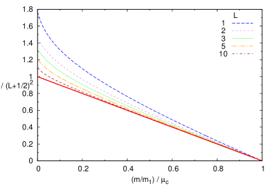
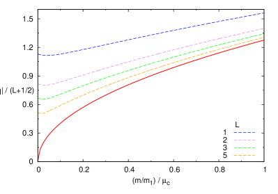
Figure 1: Mass-ratio dependencies of $\tilde{\gamma}^{2}$ (a) and $q$ (b) for two identical fermions (bosons) if $L$ is odd (even). In (a) the curves correspond to $L=1,2,3,5,10$ (top to bottom) and the uppermost solid line depicts the dominant asymptotic law $\tilde{\gamma}^{2}/(L+1/2)^{2}\approx 1-\frac{m/m_{1}}{\mu_{c}}$ for $L\to\infty$ as follows from Eqs. (45). In (b) the curves correspond to $L=1,2,3,5$ (top to bottom) and the uppermost solid line depicts the dominant asymptotic law $|q|/(L+1/2)^{2}\approx 2/(1+u0)\sqrt{\frac{m/m_{1}}{\mu_{c}}}$ for $L\to\infty$ as follows from Eqs. (45) and (47).

The explicit equations for $\mu_{c}$, $\mu_{e}$, and $\mu_{r}$ (in terms of corresponding $\omega_{c}$, $\omega_{e}$, and $\omega_{r}$) are obtained by simplification of Eq. (10) and using Eq. (37)

$$\Gamma^{2}\left(\frac{L}{2}+1\right)\cos\omega_{c}-\left(\frac{\sin\omega_{c}}{2}\right)^{L}\left(\frac{1}{\sin\omega_{c}}\frac{d}{d\omega_{c}}\right)^{L}\frac{\omega_{c}}{\sin\omega_{c}}=0\ ,$$ (18a)

$$(L+1/2)\sqrt{\sin\omega_{e}}\cos\omega_{e}-\left(\tan\frac{\omega_{e}}{2}\right)^{L+1/2}=0\ ,$$ (18b)

$$2^{L-1}(L+1)\Gamma^{2}\left(\dfrac{L+1}{2}\right)\cos\omega_{r}+(\sin\omega_{r})^{L}\left(\frac{1}{\sin\omega_{r}}\dfrac{d}{d\omega_{r}}\right)^{L}\left(\omega_{r}\cot\omega_{r}\right)=0\ .$$ (18c)

A list of $\mu_{r}$, $\mu_{e}$, and $\mu_{c}$ for $L=\overline{0,10}$ is given in Table 1.

Table 1: The critical mass ratios $\mu_{r}$, $\mu_{e}$, and $\mu_{c}$ corresponding to $\gamma=1$, $1/2$, and $0$ for $L=\overline{0,10}$ and $S=(-)^{L}$, i. e., odd (even) $L$ if identical particles are fermions (bosons).

$L$	$\mu_{r}$	$\mu_{e}$	$\mu_{c}$	$|q_{r}|$	$|q_{e}|$	$|q_{c}|$
$0$	-	-	0	-	-
$1$	8.6185769247	12.313099346	13.606965698	2.0918978	2.2795930	2.3425382
$2$	32.947611782	37.198932993	38.630158395	3.3002049	3.4491653	3.4981899
$3$	70.070774958	74.510074146	75.994494341	4.5462732	4.6644862	4.7034648
$4$	119.73121698	124.25484012	125.76463572	5.8053122	5.9020644	5.9340526
$5$	181.86643779	186.43468381	187.95835509	7.0703622	7.1518593	7.1788515
$6$	256.455446	261.0500269	262.582047	8.346725	8.420731	8.445263
$7$	343.489658	348.1010286	349.638439	9.615754	9.679806	9.701066
$8$	442.965041	447.5877601	449.128842	10.88657	10.94303	10.96179
$9$	554.879529	559.5102570	561.053949	12.15857	12.20906	12.22585
$10$	679.231936	683.8685388	685.414150	13.43140	13.47707	13.49225

In the opposite case $S=(-)^{L+1}$, i. e., for even (odd) $L>0$ if identical particles are fermions (bosons), $\tilde{\gamma}^{2}$ monotonically increases from $(L+1)^{2}$ to $(L+2)^{2}$ with increasing $0<m/m_{1}<\infty$, while for fermions in the $L=0$ state $\tilde{\gamma}^{2}$ monotonically increases from $4$ to $16$.

It is not surprising that the parameter $\tilde{\gamma}$, which essentially determines the solution for $\rho\to 0$, naturally appears in papers Minlos (2011b, 2012, 2014a, 2014b); Correggi et al. (2012, 2015a); Michelangeli and Ottolini (2018); Becker et al. (2018); Castin and Tignone (2011) treating the problem by means of the momentum-space integral equation. Within the framework of this approach, the equation for $\tilde{\gamma}$ (in adapted notations) reads

$$\dfrac{(-)^{L}}{\pi\cos\omega}\int_{-1}^{1}dxP_{L}(x)\int_{0}^{\infty}\dfrac{dyy^{\tilde{\gamma}}}{y^{2}+2xy\sin\omega+1}=1\ ,$$ (19)

where $P_{L}(x)$ is the Legendre polynomial. Evaluation of the inner integral and change of variables $\sin z=-x\sin\omega$ gives

$$\dfrac{2}{\sin\tilde{\gamma}\pi\sin 2\omega}\int_{-\omega}^{\omega}dzP_{L}\left(\dfrac{\sin z}{\sin\omega}\right)\sin[\tilde{\gamma}(\pi/2-z)]=1\ .$$ (20)

This equation is equivalent of. (10) for $\rho=0$.

The coupling terms of HREs are readily deduced in the asymptotic region $\rho\to\infty$ from the expansion of $\gamma_{n}^{2}(\rho)$ and analytical expressions (15)–(17), which gives $Q_{nm}(\rho)=O(\rho^{-2})$ and $P_{nm}=O(\rho^{-4})$ for all $n,m$, except the lowest-channel couplings for $a>0$, which are given by $P_{11}(\rho)=\frac{1}{4\rho^{2}}+O(\rho^{-6})$, $P_{1n}(\rho)=O(\rho^{-7/2})$ and $Q_{1n}(\rho)=O(\rho^{-5/2})$. Thus, the asymptotic form of the channel potentials is

$$V_{n}(\rho)=\frac{[L+2n-1-\mathrm{sgn}(a)]^{2}-1/4}{\rho^{2}}+O(\rho^{-3})\ ,$$ (21)

except of the lowest one for $a>0$, which is given by

$$V_{1}(\rho)=-1+\frac{L(L+1)}{\rho^{2}}+O(\rho^{-4})\ .$$ (22)

II Boundary conditions for generalized Coulomb problem

For the generalized Coulomb problem the effective potential contain two singular terms $(\tilde{\gamma}^{2}-1/4)/\rho^{2}+q/\rho$. It is necessary to analyse

$$\left(\frac{d^{2}}{d\rho^{2}}-\frac{\tilde{\gamma}^{2}-1/4}{\rho^{2}}-\frac{q}{\rho}+E\right)f(\rho)=0$$ (23)

at small $\rho$. There are two solutions at $\rho\to 0$, which leading order terms are $\sim\rho^{1/2\pm\tilde{\gamma}}$.

For $\tilde{\gamma}^{2}\geq 1$, $f(\rho)\sim\rho^{1/2+\tilde{\gamma}}$ is the only square-integrable solution for $\rho\to 0$ (the appropriate boundary condition $f(\rho)\to 0$). In contrast, for $\tilde{\gamma}^{2}<1$ both solutions $\sim\rho^{1/2\pm\tilde{\gamma}}$ at $\rho\to 0$ are square-integrable. Therefore, for unambiguous formulation of the three-body problem near $\rho\to 0$ it is necessary to fix the linear combination of these solutions in $f(\rho)$, which requires the additional three-body parameter. If $\tilde{\gamma}^{2}<0$ there is an Efimov situation, namely, both square-integrable solutions at $\rho\to 0$ are oscillating. And it is already known that the additional three-body regularizational parameter (called the Efimov parameter) is needed to fix the wave function in the TCP that results in energy spectrum exponentially depending on the level’s number $E=-e^{-\frac{2\pi}{|\tilde{\gamma}|}n}$ Case (1950). Furthermore, one should consider the remaining case $0\leq\tilde{\gamma}^{2}<1$. As follow from Eq. (23), on the interval $1/2<\tilde{\gamma}<1$ ($\mu_{r}>m/m_{1}>\mu_{e}$) one has to take into account also the next to leading order term in the second square-integrable solution $\sim\rho^{1/2-\tilde{\gamma}}$, namely, $q\rho^{3/2-\tilde{\gamma}}/(1-2\tilde{\gamma})$, because it is of the same order as the first square-integrable solution $\sim\rho^{1/2+\tilde{\gamma}}$. As a result, denoting the additional three-body parameter via $b$, the three-body boundary condition for the channel function $f(\rho)$ read as

$$f(\rho)\xrightarrow[\rho\to 0]{}\rho^{1/2+\tilde{\gamma}}-\operatorname{sgn}(b)|b|^{2\tilde{\gamma}}\rho^{1/2-\tilde{\gamma}}\left[1+q\rho/(1-2\tilde{\gamma})\right]\$$ (24)

for all $\tilde{\gamma}$ except for $\tilde{\gamma}=1/2$. The last term in the square brackets ($\sim q\rho$) is necessary only for $1/2<\tilde{\gamma}<1$ and can be omitted for $0<\tilde{\gamma}<1/2$. In the limit $\tilde{\gamma}\to 0$, the boundary condition (24) takes a simple form

$$f(\rho)\xrightarrow[\rho\to 0]{}\rho^{1/2}\log(\rho/b)\ ,$$ (25)

where only $b>0$ is allowed. In the specific case $\tilde{\gamma}=1/2$ there are two square-integrable solutions at $\rho\to 0$, namely, $\rho$ and $1+q\rho\log\rho$. The boundary condition reads

$$f(\rho)\xrightarrow[\rho\to 0]{}\rho-b(1+q\rho\log\rho)\ .$$ (26)

It is suitable to write the three-body boundary conditions in the alternative form, viz., in terms of the derivative of the function $f(\rho)$. The boundary condition for $0\leq\tilde{\gamma}<1$ $\&$ $\tilde{\gamma}\neq 1/2$ reads

$$\lim_{\rho\to 0}\left(\rho^{1-2\tilde{\gamma}}\frac{d}{d\rho}+\operatorname{sgn}(b)\frac{2\tilde{\gamma}}{|b|^{2\tilde{\gamma}}}\right)\frac{\rho^{\tilde{\gamma}-1/2}}{1-2\tilde{\gamma}+q\rho}f(\rho)=0\ ,$$ (27)

which is equivalent to Eq. (24). In the limit $\tilde{\gamma}\to 0$ the boundary condition, which is equivalent to Eq. (25), takes the form

$$\lim_{\rho\to 0}\left(\rho\frac{d}{d\rho}-\frac{1}{\log(\rho/b)}\right)\rho^{-1/2}f(\rho)=0\ ,$$ (28)

where only $b>0$ is allowed. In the specific case of $\tilde{\gamma}=1/2$ the boundary condition

$$\lim_{\rho\to 0}\left(\frac{d}{d\rho}+\frac{1}{b}\right)\frac{f(\rho)}{1+q\rho\log\rho}=0\$$ (29)

is equivalent to Eq. (26). Notice that the boundary condition for $\tilde{\gamma}=0$ determined by Eq. (24) or Eq. (28) is similar to that for the $2D$ zero-range model Kartavtsev and Malykh (2006), whereas for $\tilde{\gamma}=1/2$ the boundary condition of the form (26) or (29) is similar to that for a sum of the zero-range and Coulomb potentials as in Yakovlev and Gradusov (2013). Usage $\ln(|q|\rho)$ instead of $\ln\rho$ in (26) for $\tilde{\gamma}=1/2$ simply means the redefinition of the parameter $b$ on $\tilde{b}=b/(1+bq\ln|q|)$, then it coincides with Albeverio et al. (1983).

The usage of the boundary conditions (24)-(26), or (27)-(29) with arbitrary three-body parameter $b$ (with dimension of length) determine the general zero-range three-body potential. The relation of the general approach for zero-range three-body potential with particular examples of the shrinking three-body potentials is given in Appendix B.

III Self-ajoint Hamiltonian

Singular terms in the HREs (13) for $\rho\to 0$ shows that one should apply the analysis of Sec. II to formulate of the three-body boundary conditions. The wave function $\Psi$ near the TCP ($\rho\to 0$) is basically determined by the most singular terms in the effective potential in the first channel $V_{1}(\rho)$ (14), i. e., $(\tilde{\gamma}^{2}-1/4)/\rho^{2}+q/\rho$ and the corresponding channel function $f_{1}(\rho)$. In the following the general analyse of Sec. II will be applied to the first channel $f(\rho)\equiv f_{1}(\rho)$. Therefore, using the analysis of behavior of $\tilde{\gamma}$ and $q$ as functions of mass ratios and using the way of regularization of the wave functions of Sec. II in dependence on $\tilde{\gamma}$, one comes to the conclusions. First, one finds that for the mass-ratios $m/m_{1}\leq\mu_{r}$ and $S=(-1)^{L}$ (odd or even $L$ if identical particles are fermions or bosons, respectively) and for any mass ratio and $S=(-1)^{L+1}$ (even or odd $L$ if identical particles are fermions or bosons, respectively) the Hamiltonian is self-ajoint, due to $\tilde{\gamma}>1$. One can use the zero boundary condition in TCP. Second, notice that the Efimov situation corresponds to $m/m_{1}\geq\mu_{c}$ and $S=(-1)^{L}$ due to $\tilde{\gamma}\leq 0$. The way of regularisation in the TCP to make the Hamiltonian self-ajoint is well investigated in the literature. Third, the most interesting case $0\leq\tilde{\gamma}<1$ corresponds to the mass-ratios $\mu_{r}<m/m_{1}\leq\mu_{c}$ and $S=(-1)^{L}$ (odd or even $L$ if identical particles are fermions or bosons, respectively). To make the self-ajoint Hamiltonian one need to use the corresponding boundary condition in the TCP of the form (24)–(26), or (27)–(29) for the channel function in the first channel. Only this case will considered below.

Remark that the boundary condition in Michelangeli and Ottolini (2018) coincides with Eq. (24) or (27) if one omit the term $\sim q$, that means that the boundary condition in Michelangeli and Ottolini (2018) can be used only for $0\geq\tilde{\gamma}\geq 1/2$. The three-body parameter $b$ ($R_{t}$ in Gao et al. (2015)) and the three-body boundary condition was introduced also in paper Gao et al. (2015) devoted to calculation of the third virial coefficient, where only positive value of $b$ is taken into account and the term $\sim\rho^{-1}$ is not considered. For $0\leq\tilde{\gamma}<1/2$ this term is of the principal importance. Generally, the three-body parameter $b$ and the boundary condition can depend not only on $L$, but on it’s projection $M$. Nevertheless, in real situation it doesn’t seem probable.

It is of interest to write boundary conditions for the total wave function $\Psi$. Namely, as in Kartavtsev and Malykh (2016), the required expressions can be written as

$$\Psi\sim(\rho^{\tilde{\gamma}-2}\mp|b|^{2\tilde{\gamma}}\rho^{-\tilde{\gamma}-2})\Phi_{1}(0,\Omega)$$ (30)

or

$$\lim_{\rho\to 0}\left(\rho^{1-2\tilde{\gamma}}\frac{d}{d\rho}\pm\frac{2\tilde{\gamma}}{|b|^{2\tilde{\gamma}}}\right)\rho^{2+\tilde{\gamma}}\Psi=0\ ,$$ (31)

if $0<\tilde{\gamma}<1/2$ that equivalent to (24), (27). On the other hand, the boundary condition for $1/2<\tilde{\gamma}<1$ becomes cumbersome due to necessity to keep in the expansion of $\Psi$ for $\rho\to 0$ also the term $\sim\rho^{-\tilde{\gamma}-1}$, which includes an additional function of hyper-angles.

IV Bound-state energies

IV.1 Infinite two-body scattering length

In the limit $|a|\to\infty$, $\gamma_{n}^{2}(\rho)$ in (10) do not dependent on $\rho$ and all the terms $Q_{nm}(\rho)$ and $P_{nm}(\rho)$ vanish. Therefore, HREs (13) decouple and the three-body bound-state energies is a solution of one HRE, in which $\gamma^{2}(\rho)\equiv\tilde{\gamma}^{2}$. For $b>0$, there is one bound state whose energy is $E=-4b^{-2}\left[-\Gamma(\tilde{\gamma})/\Gamma(-\tilde{\gamma})\right]^{1/\tilde{\gamma}}$ and eigenfunction is $f(\rho)=\rho^{1/2}K_{\tilde{\gamma}}(\sqrt{-E}\rho)$, where $K_{\nu}(x)$ is the modified Bessel function. If $b\to\infty$, the bound state goes to the threshold $E\to 0$ and turning into the virtual state. Then, for $b<0$ it’s energy is given by the above expression. Also, the above expressions for $E$ and $f(\rho)$ describe the properties of the bound deep state, which exists for $|a|\gg b$.

IV.2 Simple model

As a preliminary consideration, it is worthwhile to give qualitative description of the energy spectrum as function of $b$ and $m/m_{1}$ within the framework of the simple model. The model is equivalent to the generalised Coulomb problem incorporating the zero-range interaction and is based on splitting of the Hamiltonian into the singular part $(\gamma^{2}-1/4)/\rho^{2}+q/\rho$ as $\rho\to 0$ and the remaining one, which is simply taken as a constant $\epsilon(\gamma)$ smoothly dependent on $m/m_{1}$. Retaining one equation containing the most singular terms from the system (13), one comes to the equation

$$\left(\frac{d^{2}}{d\rho^{2}}-\frac{\gamma^{2}-1/4}{\rho^{2}}-\frac{q(\gamma)}{\rho}+E-\epsilon(\gamma)\right)f(\rho)=0$$ (32)

complimented by one of the boundary conditions (24), (25), and (26). Similar to Kartavtsev and Malykh (2016), the solution of generalised Coulomb problem leads to the eigenenergy equations

$$\left(2\kappa|b|\right)^{2\gamma}=\displaystyle\mp\frac{\Gamma(2\gamma)\Gamma\left(1/2-\gamma+q/(2\kappa)\right)}{\Gamma(-2\gamma)\Gamma\left(1/2+\gamma+q/(2\kappa)\right)}\quad 0\leq\gamma<1,\gamma\neq 1/2,$$ (33a)

$$\ln(2\kappa b)+\psi\left(\frac{1}{2}+\frac{q}{2\kappa}\right)+2\gamma_{C}=0,\qquad\qquad\qquad\gamma=0,\quad b\geq 0,$$ (33b)

$$\frac{1}{q}\left(\frac{1}{b}-\kappa\right)-\ln\left(\frac{|q|}{2\kappa}\right)+\psi\left(1+\frac{q}{2\kappa}\right)+2\gamma_{C}-1=0,\quad\gamma=1/2,$$ (33c)

where $\kappa=\sqrt{\epsilon(\gamma)-E}$, $\psi(x)$ is the digamma function and $\gamma_{C}\approx 0.5772$ is the Euler–Mascheroni constant. Eq. (33b) can be obtained from Eq. (33a) by taking the limit $\gamma\to 0$ for any $b\geq 0$. Recall that the parameter $b$ in Eq. (33c) is defined in Eq. (26) differently.

As follows from Eqs. (33), all the bound-state energies monotonically increase with increasing $b$; moreover, one bound state arises at $-\infty$ if $b$ passes through zero. Particularly, in two limits $b=0$ and $b\to\infty$ one obtains the Coulomb spectrum for energies

$$E_{n}^{(b=0,\infty)}(\gamma)=-\frac{q^{2}(\gamma)}{[2(n+s\gamma)+1]^{2}}+\epsilon(\gamma)\ ,$$ (34)

where $s=\pm 1$ corresponds to $b=0$ ($s=+1$) and $b\to\infty$ ($s=-1)$. In each case the index $n\geq 0$ enumerating energy levels is limited either by the condition $n>-s\gamma-1/2$ if $a>0$ ($q<0$) or $n<-s\gamma-1/2$ if $a<0$ ($q>0$). The maximum value of $n$ is restricted by $E_{n}^{(b=0,\infty)}(\gamma)<-1$ if $a>0$ or $E_{n}^{(b=0,\infty)}(\gamma)<0$ if $a<0$. The Eq. (34) is valid for any mass ratio including the exceptional value $m/m_{1}\to\mu_{e}$ ($\gamma\to 1/2$).

The specific feature of the Coulomb spectrum (34) is a degeneracy of energy levels for integer and half-integer value of $\gamma$, i.e., at $m/m_{1}\to\mu_{c}$ ($\gamma\to 0$), $m/m_{1}\to\mu_{e}$ ($\gamma\to 1/2$), and $m/m_{1}\to\mu_{r}$ ($\gamma\to 1$). In the case $a>0$, $E_{n}^{(0)}(0)=-q^{2}(0)/(2n+3)^{2}+\epsilon(0)$ ($n\geq 0$) coincides with $E_{n}^{(\infty)}(0)$ for $m/m_{1}\to\mu_{c}$ ($\gamma\to 0$), $E_{n}^{(0)}(1/2)=-q^{2}(1/2)/(2n+3)^{2}+\epsilon(1/2)$ ($n\geq 0$) coincides with $E_{n+1}^{(\infty)}(1/2)$ for $m/m_{1}\to\mu_{e}$ ($\gamma\to 1/2$), $E_{n}^{(0)}(1)=-q^{2}(1)/(2n+3)^{2}+\epsilon(1)$ ($n\geq 0$) coincides with $E_{n+2}^{(\infty)}(1)$ for $m/m_{1}\to\mu_{r}$ ($\gamma\to 1$). The ground state $E_{0}^{(\infty)}(\gamma)$ tends to $-\infty$ for $m/m_{1}\to\mu_{e}$ ($\gamma\to 1/2$) and disappears for $m/m_{1}\leq\mu_{e}$ ($\gamma\geq 1/2$). For $m/m_{1}<\mu_{e}$ ($\gamma>1/2$) $E_{1}^{(\infty)}(\gamma)$ becomes a ground state and for $m/m_{1}\to\mu_{r}$ ($\gamma\to 1$) tends to a finite value $-q^{2}(1)+\epsilon(1)$, which is not degenerate with any $E_{n}^{(0)}(1)$. In the case $a<0$, there is only $E_{0}^{(\infty)}(\gamma)$ in the interval $\mu_{r}<m/m_{1}<\mu_{e}$, which tends to $-q^{2}(1)+\epsilon(1)$ for $m/m_{1}\to\mu_{r}$ ($\gamma\to 1$) and to $-\infty$ for $m/m_{1}\to\mu_{e}$ ($\gamma\to 1/2$). One should note that both $E_{0}^{(\infty)}(1)$ for $a<0$ and $E_{1}^{(\infty)}(1)$ for $a>0$ coincides in the limit $m/m_{1}\to\mu_{r}$ ($\gamma\to 1$).

Furthermore, in the case $a>0$, the energy of the $n^{th}$ level ($n\geq 0$) for any $b\leq 0$ converges to $E_{n}^{(0)}(0)=-q^{2}(0)/(2n+3)^{2}+\epsilon(0)=E_{n}^{(\infty)}(0)$ in the limit $m/m_{1}\to\mu_{c}$ ($\gamma\to 0$). For $m/m_{1}=\mu_{c}$ ($\gamma=0$) the ground-state energy increases from $-\infty$ to $E_{0}^{(0)}(0)$ with increasing $b$ from zero to infinity, while the $n^{th}$ level increases from $E_{n-1}^{(0)}(0)$ to $E_{n}^{(0)}(0)$, and the upper level disappears at the threshold for some finite value $b>0$. If the mass ratio tends to the next specific value $m/m_{1}\to\mu_{e}$ ($\gamma\to 1/2$), for any $b$ all the energies converge to $E_{n}^{(0)}(1/2)=-q^{2}(1/2)/(2n+3)^{2}+\epsilon(1/2)=E_{n+1}^{(\infty)}(1/2)$ ($n\geq 0$), and additionally the ground-state energy for $m/m_{1}>\mu_{e}$ tends to $-\infty$ in the same limit. If the mass ratio tends to $m/m_{1}\to\mu_{r}$ ($\gamma\to 1$), for any $b$ the energies converge to either $E_{1}^{(\infty)}(1)=-q^{2}(1)+\epsilon(1)$ or $E_{n}^{(0)}(1)=-q^{2}(1)/(2n+3)^{2}+\epsilon(1)=E_{n+2}^{(\infty)}(1)$ ($n\geq 0$). In the case $a<0$, for $m/m_{1}\to\mu_{r}$ ($\gamma\to 1$) the energies converge to $E_{0}^{(\infty)}$ for any $b$. The descriptions of the spectrum by means of the simple model are in agreement with numerical calculation as can be seen in Fig. 2.

A comparison of the ground and excited states energies for $b=0$ Kartavtsev and Malykh (2007b) with Eq. (34) shows that reasonable agreement could be obtained for $\epsilon$ about $-0.4\div-0.6$ for $1\leq L\leq 5$. Using the above estimate for the constant $\epsilon$, one finds that for $a>0$ there are about $L+1$ levels below the two-body threshold ($E\leq-1$) if $b=0$ and about $L+2$ levels if $b\to\infty$, while for $a<0$ there is one level below the three-body threshold ($E\leq 0$) if $b\to\infty$ (see Fig. 2).

IV.3 Numerical results for $L=1\div 5$

The mass-ratio dependence of the three-body energies for angular momentum $L\leq 5$ ($L^{P}=1^{-},\,3^{-},\,5^{-}$ or $L^{P}=2^{+},\,4^{+}$ if two identical particles are fermions or bosons, respectively) is determined on the mass ratio interval $\mu_{r}(L^{P})<m/m_{1}\leq\mu_{c}(L^{P})$ ($1>\gamma\geq 0$) by solving a system of HREs (13) complemented by the special boundary conditions (24) or (25) or (26) in the TCP and the zero asymptotic boundary condition, $f_{n}(\rho)\to 0$ as $\rho\to\infty$. Solution of up to eight HREs provides five - six digits in the calculated energy. The results of the calculations are shown in Fig. 2 for $L^{P}=1^{-},\ 2^{+},\ 3^{-}$ in the cases of positive and negative two-body scattering length $a$.

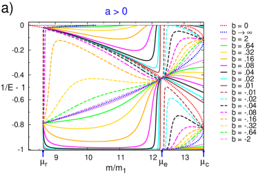
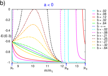
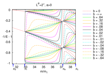
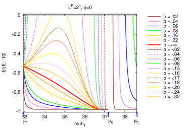
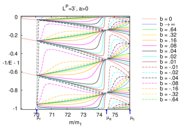
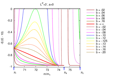
Figure 2: Bound-state energies $E$ for three-body system with two identical fermions (bosons) in $L^{p}=1^{-},\,3^{-}$ (for $L^{p}=2^{+}$) states as a function of $m/m_{1}$ and $b$. The energies for the two-body scattering length $a>0$ and $a<0$ are presented in panel a and panel b, respectively, and the energy axis scaled to map $-\infty<E<-1$ (panel a) and $-\infty<E<0$ (panel b) to the interval $(-1,0)$. Values $\mu_{r}$, $\mu_{e}$ and $\mu_{c}$ correspond to $\gamma=1$, $1/2$ and $0$.

For positive two-body scattering length it turns out that the number of the bound states increases with increasing $L$, but, qualitatively, energy dependence on $m/m_{1}$, $b$ is similar for different $L$. Namely, one obtain the spider-like plot with monotonic increasing of the bound-state energies with increasing $b$ at fixed $m/m_{1}$. In fact, the bound-state energies dependence for positive and negative values of $b$ are separated of each other by the limiting mass-ratio dependences for $b=0$ and $b=\infty$, and by the critical value of mass ratio $\mu_{e}(L^{P})$. Moreover, limiting dependences of the three-body bound-state energies monotonically decrease for $b=0$ and monotonically increase for $b=\infty$ with increasing mass ratio as illustrated in Fig. 2. When $m/m_{1}$ tends to either of specific values $\mu_{r}(L^{P})$, $\mu_{e}(L^{P})$, and $\mu_{c}(L^{P})$, the three-body energies for $b=0$ coincide with those for $b\to\infty$. Besides, for $b\to\infty$ there is the ground state, which energy tends to the finite value as $m/m_{1}\to\mu_{r}(L^{P})$ and to minus infinity as $m/m_{1}\to\mu_{e}(L^{P})$. The three-body energies for $b\neq 0,\,b\neq\infty$ tends to those for $b\to\infty$ in the limit of mass ratios $\mu_{r}(L^{P})$, $\mu_{e}(L^{P})$, and $\mu_{c}(L^{P})$ except the positive values of $b$ in the limit $m/m_{1}\to\mu_{c}(L^{P})$. The calculated three-body energies in three limits $\mu_{r}(L^{P})$, $\mu_{e}(L^{P})$, and $\mu_{c}(L^{P})$ are presented in Tab. 2.

For negative two-body scattering length, the energy dependence on $m/m_{1}$, $b$ is similar for different $L^{P}$ sectors: the only bound state exists for any positive value of $b$ and some negative values of $b$ on the mass-ratio interval $\mu_{r}(L^{P})<m/m_{1}\leq\mu_{e}(L^{P})$, whereas on the interval $\mu_{e}(L^{P})<m/m_{1}\leq\mu_{c}(L^{P})$ the bound state exists only for small enough positive values of $b$. Three-body bound-state energies for limiting value of the mass ratio $\mu_{r}(L^{P})$ are presented as underlined numbers in the Tab. 2. They considers with the same numbers for positive $a$.

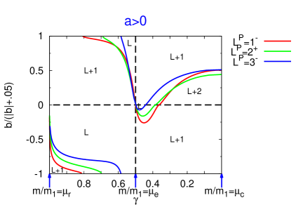
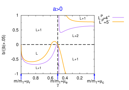
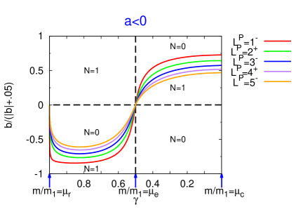
Figure 3: A number of bound states in $L^{P}$ sector in each domain of the $\gamma$ – $b$ plane for the two-body scattering length $a>0$ and $a<0$. Solid line: critical three-body parameter $b_{c}(\gamma)$, for which the bound-state energy coincides with the threshold. Dashed (black) lines: domain boundaries determined by $\gamma=1/2$ ($m/m_{1}=\mu_{e}$) and $b=0$. Values $\gamma=1$, $1/2$ and $0$ correspond to $\mu_{r}$, $\mu_{e}$ and $\mu_{c}$.

Table 2: Bound-state energies ($E_{i}$) for $b=0$ and $b\to\infty$ at the critical values $m/m_{1}\to\mu_{r}$, $m/m_{1}=\mu_{e}$ and $m/m_{1}=\mu_{c}$ and $a>0$. The entry for $E_{0}$ and $m/m_{1}\to\mu_{r}$ represent also the energies in the case $a<0$. Two identical particles are fermions (bosons) if parity is odd (even).

$L^{P}$	$1^{-}$	$2^{+}$	$3^{-}$	$4^{+}$	$5^{-}$
			$m/m_{1}\to\mu_{r}$
$-E_{0}$	4.7473	11.3111	21.1146	34.1622	50.4592
$-E_{1}$	1.02090	1.68551	2.77004	4.22117	6.03404
$-E_{2}$	-	1.02748	1.35435	1.85585	2.49935
$-E_{3}$	-	-	1.03169	1.24191	1.54982
$-E_{4}$	-	-	-	1.03374	1.18686
$-E_{5}$	-	-	-	-	1.03485
			$m/m_{1}=\mu_{e}$
$-E_{0}$	1.74397	3.42540	5.90130	9.17834	13.26233
$-E_{1}$	-	1.27038	1.86005	2.66958	3.68670
$-E_{2}$	-	-	1.16759	1.49716	1.93501
$-E_{3}$	-	-	-	1.12596	1.34729
$-E_{4}$	-	-	-	1.00088	1.10398
$-E_{5}$	-	-	-	-	1.00503
			$m/m_{1}=\mu_{c}$
$-E_{0}$	5.89543	12.67370	22.57676	35.67806	52.00787
$-E_{1}$	1.13767	1.84445	2.93742	4.39267	6.20802
$-E_{2}$	-	1.07220	1.41376	1.91816	2.56267
$-E_{3}$	-	-	1.05497	1.27207	1.58177
$-E_{4}$	-	-	-	1.04795	1.20485
$-E_{5}$	-	-	-	-	1.04442

IV.4 Critical conditions

Dependence of the number of bound states on the mass ratio and the three-body parameter

For better illustration of the energy spectrum it is useful to construct the ”Phase Diagram” representing appearance of the bound state in the plane of two parameters $m/m_{1}$ and $b$. In this respect it is necessary to take into account the following. If $b$ passes over $b=0$ from negative to positive values, one additional bound state arises at $-\infty$ and it’s energy increases with increasing $b$, i.e., a number of bound states $N(b)$ increases by unity for $b>0$ ($N(b\geq 0)=N(b<0)+1$). Furthermore, if the mass ratio goes across $\mu_{e}$ from lower to higher values and $b\neq 0$, one more bound state should appear for $a>0$ and disappear for $a<0$. If $b$ passes critical line $b_{c}(m/m_{1})$ (for which the bound-state energy $E$ coincides with the threshold) from higher to lower values of $b$ one more bound state should appear both for positive and negative value of $a$. The critical line $b_{c}(m/m_{1})$ goes from the point $b_{c}=0$, $m/m_{1}=\mu_{r}$ through the point $b_{c}=0$, $m/m_{1}=\mu_{e}$ to the point $m/m_{1}=\mu_{c}$, $b_{c}=b_{f}>0$. Therefore, the lines $b_{c}(m/m_{1})$, $b=0$, and $m/m_{1}=\mu_{e}$ form boundaries of the domains of the definite number of bound states in the $m/m_{1}$ – $b$ plane as presented in Fig. 3.

Elaborate calculations were carried out to determine the critical parameter $b_{c}(m/m_{1})$, for which the bound-state energy coincides with the threshold. Namely, $b_{c}(m/m_{1})$ was determined by solving the eigenvalue problem for HREs at the two-body threshold $E=-1$ for the two-body scattering length $a>0$ and at the three-body threshold $E=0$ for $a<0$. Existence of bound states at the threshold energy follows from the power decay of the channel function $f_{1}(\rho)$ for $\rho\to\infty$, namely, $f_{1}(\rho)\sim\rho^{-L}$ for $a>0$ and $f_{1}(\rho)\sim\rho^{-L-3/2}$ for $a<0$, that is related with asymptotic behaviour of the first channel effective potential (22) and (21) for positive and negative $a$, respectively. As usual, the bound state at the threshold turns to a narrow resonance under small variations of $m/m_{1}$ and $b$.

Few points of the dependence $b_{c}(m/m_{1})$ are of special interest, viz., one finds for $a>0$ that $b_{c}=0$ at largest mass ratios presented in upper part of Tab. 3 (namely, $m/m_{1}\approx 12.91742$, $37.7662$, $74.8233$, $124.168$, $185.829$ for $L^{P}=1^{-},\,2^{+},\,3^{-},\,4^{+},\,5^{-}$, respectively), $b_{c}\to\pm\infty$ at mass ratios presented in lower part of Tab. 3; $b_{c}\approx 0.0517$, $0.0416$, $0.0547$, $0.0897$, $0.177$ for $1^{-},\,2^{+},\,3^{-},\,4^{+},\,5^{-}$, respectively, at the mass ratio $m/m_{1}=\mu_{c}$; and $b_{c}(m/m_{1})$ has a local minimum $b_{c}\approx-0.0175$ at $m/m_{1}\approx 12.550$ for $L^{P}=1^{-}$ sector, $b_{c}\approx-0.0095$ at $m/m_{1}\approx 37.420$ for $L^{P}=2^{+}$ sector, $b_{c}\approx-0.0038$ at $m/m_{1}\approx 74.635$ for $L^{P}=3^{-}$ sector, $b_{c}\approx-0.0009$ at $m/m_{1}\approx 124.217$ for $L^{P}=4^{+}$ sector, $b_{c}\approx-0.0062$ at $m/m_{1}\approx 186.143$ for $L^{P}=5^{-}$ sector. Similarly, one finds for $a<0$ that $b_{c}\approx 0.13620$, $0.09065$, $0.06725$, $0.05324$, $0.04398$ for $L^{P}=1^{-},\,2^{+},\,3^{-},\,4^{+},\,5^{-}$, respectively, at $m/m_{1}=\mu_{c}$; and $b_{c}(m/m_{1})$ has a local minimum $b_{c}\approx-0.2501$ at $m/m_{1}\approx 10.15$ for $L^{P}=1^{-}$, $b_{c}\approx-0.1634$ at $m/m_{1}\approx 34.758$ for $L^{P}=2^{+}$, $b_{c}\approx-0.1201$ at $m/m_{1}\approx 71.980$ for $L^{P}=3^{-}$, $b_{c}\approx-0.0947$ at $m/m_{1}\approx 121.678$ for $L^{P}=4^{+}$, $b_{c}\approx-0.0780$ at $m/m_{1}\approx 183.837$ for $L^{P}=5^{-}$.

Table 3: The critical values $m/m_{1}$, for which the bound $L^{P}$ states arise for $b_{c}(m/m_{1})=0$ and $b_{c}(m/m_{1})\to\infty$. Two identical particles are fermions (bosons) if parity is odd (even).

$L^{P}$	$1^{-}$	$2^{+}$	$3^{-}$	$4^{+}$	$5^{-}$
			$b=0$
	8.17259	22.6369	43.3951	70.457	103.823
	12.91742	31.5226	56.1652	87.027	124.155
	-	37.7662	67.3352	102.488	143.664
	-	-	74.8233	115.536	161.402
	-	-	-	124.168	176.097
	-	-	-	-	185.829
			$b\to\infty$
	10.2948	35.9163	73.9853	124.3660	187.056

Solution in the specific points $m/m_{1}=\mu_{e},\mu_{c}$

A noticeable feature of the problem near $m/m_{1}=\mu_{e}$ ($\gamma=1/2$) is the degeneracy of energy dependences for different $b$ and a lack of continuity in the definition of $b$ (24). It is not surprising as the sgn of the most singular term in HRE alters if $\gamma$ goes across $1/2$. Due to discontinuity in the definition of $b$ the limiting values of the bound-state energy for $m/m_{1}\to\mu_{e}\mp 0$ ($\gamma\to 1/2\pm 0$) do not coincide with each other and with that calculated exactly at $m/m_{1}=\mu_{e}$ ($\gamma=1/2$). Notice also that in boundary condition (24) one could substitute $\log\rho$ with $\log(\rho/\rho_{0})$ introducing a scale $\rho_{0}$, which simply leads to redefinition of length $\tilde{b}=b/(1-b\log\rho_{0})$.

For illustration, the dependence of the bound-state energy on $b$ is calculated using boundary condition (24) and plotted in Fig. 4 for $L^{P}=1^{-}$ sector.

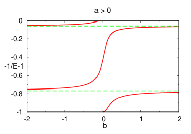
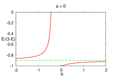
Figure 4: Bound-state energies $E$ for $L^{P}=1^{-}$ sector as a function of $b$ at $m/m_{1}=\mu_{e}$ are plotted by solid (red) lines and asymptotic limits for $b\to\infty$ are indicated by dashed (green) lines. The two-body scattering length $a>0$ (left) and $a<0$ (right) and the energy axis scaled to map $-\infty<E<-1$ (left) and $-\infty<E<0$ (right) to the interval $(-1,0)$.

The calculations for $a>0$ show that there are two bound states, one of which disappears for $-.108<b\leq 0$; for $a<0$ there is one bound state, which disappears for $-.437<b\leq 0$. In the limit $b\to\infty$ the bound-state energies tend to $-4.319$ and $-1.061$ for $a>0$ and to $-25.720$ for $a<0$. For $b=0$ definitions (24) and (24) are the same and for $a>0$ the bound-state energy takes the value $\sim-1.74397$.

The bound-state energies and critical values of $m/m_{1}$ are in general agreement with results of Kartavtsev and Malykh (2007b); Endo et al. (2011); Helfrich and Hammer (2011) for $b=0$. Only exception is that the loosely bound $L^{P}=3^{-}$ state is missed in calculation Endo et al. (2011), which solves STM equation. The critical value $m/m_{1}$ of arising a ground $L^{P}=1^{-}$ state calculated in Michelangeli and Schmidbauer (2013) is $8.1833$ that is close with $8.17259$.

V Discussion and conclusion

One of the essential points of the three-body problem under consideration is regularization, which is necessary for some values of the mass ratios. Under regularization, one introduces an additional parameter describing the wave function in the vicinity of the triple collision point. The aim of the present paper is to describe the problem for the mass-ratio interval $\mu_{r}<m/m_{1}\leq\mu_{c}$, where $\mu_{c}$ is a critical value, above which the ”falling-to-center” or Efimov and Thomas effects take place. The principal part of the problem could be considered in terms of the singular interaction $\frac{\gamma^{2}-1/4}{\rho^{2}}$, where the interval $0\leq\gamma^{2}<1$ corresponds to $\mu_{c}\geq m/m_{1}>\mu_{r}$ and for $\gamma^{2}<0$, corresponding to $m/m_{1}>\mu_{c}$, the spectrum is not bounded below. Introducing an additional parameter $b$ one selects the unique solution in the limit $\rho\to 0$. It is necessary to emphasize that to introduce the parameter $b$ for $1/4\geq\gamma^{2}<1$ one should consider also the less singular term $\sim\frac{q}{\rho}$ of the interaction.

Both total angular momentum and parity are good quantum numbers that allows one to provide a description of full spectrum by calculating the bound states separately in different $L^{P}$ sectors. If two identical particles are fermions (bosons) the bound state exists only in odd (even) states. Dependence of bound-state energies on $b$ and $m/m_{1}$ are calculated for some of $L^{P}$ sectors, a number of the bound states increases with increasing $L$ for two-body scattering length $a>0$. For negative two-body scattering length at most one bound state exists.

It is of interest to find if the described above scenario happens for the three-body problem in the mixed dimensions Nishida and Tan (2008, 2011); Lamporesi et al. (2010), in the presence of spin-orbit interaction Shi et al. (2014); Cui and Yi (2014); Shi et al. (2015) and on the lattice. The disclosed dependence on the three-body parameter should be taken into account to study of many-body properties as well, e.g., in the four-body ($3+1$) Castin et al. (2010) and ($2+2$) Endo and Castin (2015) problems. Up to now there are calculations, which show that the critical value of the mass ratio, above which the spectrum is not bounded below, are $m/m_{1}\approx 13.607$ Efimov (1973) for $2+1$ problem , $m/m_{1}\approx 13.384$ Castin et al. (2010) for $3+1$ problem and $m/m_{1}\approx 13.279$ Bazak and Petrov (2017) for $4+1$ problem. The first bound state is known to appear at $m/m_{1}\approx 8.17259$ Kartavtsev and Malykh (2007a) for $2+1$ problem, at $m/m_{1}\gtrsim 8.862$ Bazak and Petrov (2017) for $3+1$ problem and at $m/m_{1}\gtrsim 9.672$ Bazak and Petrov (2017) for $4+1$ problem. Concerning the four-body ($2+2$) problem of two fermions of one species interacting with two fermions of another species, one should mention that spectrum is bounded below, as stated in papers Endo and Castin (2015); Michelangeli and Pfeiffer (2016), and the proof of this statement for mass ratio in the interval $[0.58,1.73]$ is given in Moser and Seiringer (2018). For $N$ identical fermions interacting with a distinct particle the spectrum is bounded below for $m/m_{1}<(0.36)^{-1}\approx 2.778$ Moser and Seiringer (2017). There is another estimate in papers Correggi et al. (2012, 2015b), which give $m/m_{1}\approx 5.291$ for $N=3$, $\ m/m_{1}\approx 1.056$ for $N=8$, $\ m/m_{1}\approx.823$ for $N=9$.

Furthermore, it is of interest to study $m/m_{1}$ and $b$ dependencies of the scattering cross sections, including the three-body resonances and the recombination rate. Another point is to consider a role of the three-body parameter $b$ for $m/m_{1}$ near $\mu_{c}$ Endo et al. (2012); Gao et al. (2015) and for $m/m_{1}$ near $\mu_{r}$.

Appendix A Solutions of the auxiliary problem on a hyper-sphere

The unnormalized solutions of the equation (8) and the boundary condition (9a) is given by

$$\hskip-8.5359pt\varphi^{L}(\alpha) \sim\sqrt{\sin\alpha}Q_{\gamma-1/2}^{L+1/2}(\cos\alpha)=\sin\frac{\alpha}{2}\left(\tan\frac{\alpha}{2}\right)^{L}\frac{\Gamma(1+\gamma+L)\,\Gamma(-L-1/2)}{2\ \Gamma(\gamma-L)}\times$$

$$\times\ F\left(\frac{1}{2}-\gamma,\frac{1}{2}+\gamma;L+\frac{3}{2};\sin^{2}\frac{\alpha}{2}\right)\ ,$$ (35)

where $Q_{\nu}^{\mu}(x)$ and $F(a,b;c;x)$ are the Legendre function of second kind and hypergeometric function Bateman and Erdélyi (1953). Another form

$$\hskip-8.5359pt\varphi^{L}(\alpha) \sim(\sin\alpha)^{L+1}\ F\left(\frac{L+\gamma+1}{2},\frac{L-\gamma+1}{2};L+\frac{3}{2};\sin^{2}\alpha\right)\,$$

has been used in Castin and Tignone (2011); Gasaneo and Macek (2002). In fact, it is a finite sum, which can be written as

$$\varphi^{L}(\alpha)=\left(\sin\alpha\right)^{L+1}\left(-\frac{d}{d\cos\alpha}\right)^{L}\frac{\sin\gamma\alpha}{\sin\alpha}\,.$$ (36)

In the limit $\gamma\to n$ Eq. (36) reduces

$$\varphi^{L}(\alpha)\to\left(\sin\alpha\right)^{L+1}\left(-\frac{d}{d\cos\alpha}\right)^{L}U_{n-1}(\cos\alpha)\$$ (37)

via the Chebyshev polynomial $U_{n}(x)$, while for $\gamma=1/2$ Eq. (36) simplifies to

$$\varphi^{L}(\alpha)\sim\sin\frac{\alpha}{2}\left(\tan\frac{\alpha}{2}\right)^{L}\,.$$ (38)

To derive the transcendental equation of the form (10), one should use both $\varphi^{L}(\alpha,\rho)$ and its derivative for $\alpha=\pi/2$,

$$\varphi^{L}(\pi/2)=\frac{2^{L-1}\sin\pi\gamma}{\pi}\Gamma\left(\frac{L+\gamma+1}{2}\right)\Gamma\left(\frac{L-\gamma+1}{2}\right)\,,$$ (39)

$$\frac{d\varphi^{L}(\alpha)}{d\alpha}\Big{|}_{\alpha=\pi/2}=\varphi^{L+1}(\pi/2)\ .$$ (40)

Alternatively, one can use the recurrent relations for the Legendre functions Bateman and Erdélyi (1953) to express

$$\varphi^{L}(\alpha)=\displaystyle\left[A_{L,\gamma}(\cot\alpha)\sin\gamma\alpha+B_{L,\gamma}(\cot\alpha)\cos\gamma\alpha\right]\ ,$$ (41)

where

$$A_{L,\gamma}(x)=(\gamma-L)xA_{L-1,\gamma}(x)-(\gamma+L-1)\left[xA_{L-1,\gamma-1}(x)+B_{L-1,\gamma-1}(x)\right],$$ (42a)

$$B_{L,\gamma}(x)=(\gamma-L)xB_{L-1,\gamma}(x)+(\gamma+L-1)\left[A_{L-1,\gamma-1}(x)-xB_{L-1,\gamma-1}(x)\right],$$ (42b)

satisfy the recurrent relations, which start from $A_{0,\gamma}(x)=1$, $B_{0,\gamma}(x)=0$. Few lowest-$L$ coefficients are $A_{1,\gamma}(x)=-x$, $B_{1,\gamma}(x)=\gamma$, $A_{2,\gamma}(x)=1-\gamma^{2}+3x^{2}$, $B_{2,\gamma}(x)=-3\gamma x$, $A_{3,\gamma}(x)=3x(2\gamma^{2}-3-5x^{2})$, $B_{3,\gamma}(x)=\gamma(15x^{2}+4-\gamma^{2})$.

A.1 Leading order terms in the small-hyperradious expansion for large angular momentum $L$

For large values of $L$ one obtains $\tilde{\gamma}$ and $q$ using few terms of the expansion of hypergeometric function in (35). After substitution of the expansion in the transcendental equation (10), one obtains for $\rho=0$ up to $(L+1/2)^{-7}$

$$\cos\omega\approx\frac{u_{0}}{L+1/2}+\frac{u_{1}}{(L+1/2)^{3}}+\frac{u_{2}}{(L+1/2)^{5}},$$ (43)

where $u_{i}$ are defined as

$$\hskip-352.814ptu_{0}=e^{-u_{0}}\ ,$$ (44a)

$$u_{1}=u_{0}\left(\frac{\tilde{\gamma}^{2}-\frac{1}{4}}{2}+\frac{u_{0}^{3}}{1+u_{0}}\left(\frac{1}{4}-\frac{u_{0}}{3}\right)\right),$$ (44b)

$$u_{2}=\frac{3\tilde{\gamma}^{4}}{8} -\frac{21(1+u_{0})-6u_{0}^{2}+32u_{0}^{3}}{48(1+u_{0})}\tilde{\gamma}^{2}+$$ (44c)

$$\frac{495+1485u_{0}+1305u_{0}^{2}+1095u_{0}^{3}+3360u_{0}^{4}-912u_{0}^{5}-1744u_{0}^{6}+768u_{0}^{7}}{5760(1+u_{0})^{3}},$$

which approximately gives $u_{0}\approx 0.567143$, $u_{1}\approx-0.0637978+0.283572\,\tilde{\gamma}^{2}$, $u_{2}\approx 0.056468-0.277587\,\tilde{\gamma}^{2}+0.212679\,\tilde{\gamma}^{4}$. As $\cos\omega=\frac{\sqrt{1+2m/m_{1}}}{1+m/m_{1}}$, the connection of the critical mass ratios can be founded

$$m/m_{1}\approx\frac{2}{u_{0}^{2}}\left(l^{2}-\tilde{\gamma}^{2}\right)+\upsilon_{0}+\frac{\upsilon_{1}(\tilde{\gamma}^{2})}{l^{2}}+O(l^{-4})\ ,$$ (45)

where

$$\hskip-239.00298pt\upsilon_{0}=\displaystyle\frac{1}{2u_{0}^{2}}-\frac{5/2+u_{0}/6}{1+u_{0}}\ ,$$ (46a)

$$\upsilon_{1}(\tilde{\gamma}^{2})=\tilde{\gamma}^{2} \left(\frac{1}{u_{0}^{2}}+\frac{1+2u_{0}/3}{1+u_{0}}\right)-$$ (46b)

$$\frac{90+270u_{0}+360u_{0}^{2}+330u_{0}^{3}+525u_{0}^{4}-48u_{0}^{5}-181u_{0}^{6}-3u_{0}^{7}}{360u_{0}^{2}(1+u_{0})^{3}}$$

and $\frac{2}{u_{0}^{2}}\approx 6.2179$, $\upsilon_{0}\approx-.101098$ and $\upsilon_{1}\approx-1.04234+3.98832\,\tilde{\gamma}^{2}$. The terms of Eq. (45) up to a constant coincide with presented in Castin and Tignone (2011). Comparing these values with those given in Table 1, reveals that relative accuracy is better then $10^{-4}$ for $L=5$ and $10^{-5}$ for $L=10$. The relationship $\mu_{c}-\mu_{r}=4(\mu_{c}-\mu_{e})+O((L+1/2)^{-2})$ also follows from Eq. (45) for large $L$.

The dependence $\tilde{\gamma}^{2}(m/m_{1})$ up to an order $O((L+1/2)^{-2})$ is a linear function presented in Fig. 1. In a similar way, $q(m/m_{1})$ up to an order $O((L+1/2)^{-2})$ is a square-root dependence presented in Fig. 1 as

$$q\approx-\frac{2u_{0}\operatorname{sgn}(a)}{(1+u_{0})\cos\omega}\left(1+\frac{c_{q}}{l^{2}}+O(l^{-4})\right)\ ,$$ (47)

where $\frac{2u_{0}}{(1+u_{0})}\approx 0.7237925$, $c_{q}=\frac{1}{2}+\frac{u_{0}^{2}(3+2u_{0})}{6(1+u_{0})}\approx 0.641425$. Accuracy of (47) is about $10^{-3}$ for $L=5$ and $4\cdot 10^{-5}$ for $L=10$.

Appendix B Zero-range limit of the three-body potential

In relation with the discussion in Sec II, it is of interest to analyse zero-range model in the presence of general centrifugal and Coulomb interaction, namely, to consider the Schrödinger equation for $0\leq\gamma<1$

$$\left[-\frac{d^{2}}{d\rho^{2}}+\frac{\gamma^{2}-1/4}{\rho^{2}}+\frac{q}{\rho}+\frac{\lambda}{\rho_{0}^{2}}V(\rho/\rho_{0})-E\right]f(\rho)=0\,,$$ (48)

in the limit $\rho_{0}\to 0$. In this limit, a shape of the short-range potential $V(x)$ becomes insignificant and one comes to one-parameter description of solutions. As in Sec. II, it is natural to use the generalized scattering length $b$ defined by Eqs. (24)–(26) as a parameter. One expect that for any dependence $\lambda(\rho_{0})$ the GSL $b$ is determined by the limit

$$b\xrightarrow[\rho_{0}\to 0]{}A\,\rho_{0}\,\frac{\operatorname{sgn}\left(\lambda-\lambda_{c}\right)}{\left|\lambda-\lambda_{c}-B\,q\,\rho_{0}\right|^{\frac{1}{2\gamma}}}\ ,$$ (49)

except $\gamma=0,\ 1/2$. The constants $\lambda_{c}$, $A$, $B$ are specified by $\gamma$ and a form of the potential $V(\rho/\rho_{0})$. The values $\lambda_{c}$ have a meaning of critical values of the strength of potential, at which the threshold bound state appears. Note that, as in Section II, the Coulomb interaction plays no role in definition of $b$ for $\gamma<1/2$, therefore, for this interval Eq. (49) reduces to the simpler expression with $B=0$. The parameter $A$ is not crucial due to it can be included in definition of $b$.

In the limit $\gamma=0$, only possible positive values of $b$ are determined by

$$b\xrightarrow[\rho_{0}\to 0]{}A\,\rho_{0}\,\exp\left(\frac{1}{\lambda-\lambda_{c}}\right)\ .$$ (50)

In the special case $\gamma=1/2$,

$$b\xrightarrow[\rho_{0}\to 0]{}A\,\rho_{0}\,\left[\lambda-\lambda_{c}-B\,q\,\rho_{0}\log\rho_{0}\right]^{-1}\ ,$$ (51)

i. e., $b$ is the usual scattering length if $q=0$ and the Coulomb modified scattering length if $q\neq 0$.

From Eqs. (49)– (51), it is clear that $b=0$ for any limiting values $\displaystyle\lim_{\rho_{0}\to 0}\lambda(\rho_{0})$, except for $\lambda\xrightarrow[\rho_{0}\to 0]{}\lambda_{c}$, which correspond to existence of the bound or virtual state at zero energy. Any values of $0<|b|<\infty$ is determined by the dependence $\lambda(\rho_{0})$ in the vicinity of $\lambda_{c}$. In other words, for finite (infinite) $b$, the dependence on the potential range should be of the form

$$\lambda\xrightarrow[\rho_{0}\to 0]{}\lambda_{c}+B\,q\,\rho_{0}+\operatorname{sgn}(b)\left(A\frac{\rho_{0}}{|b|}\right)^{2\gamma}$$ (52)

where $\gamma\neq 1/2$; the term proportional to $q\rho_{0}$ can be omitted for $0<\gamma<1/2$. In the limit $\gamma\to 0$, Eq. (52) reduces to

$$\lambda\xrightarrow[\rho_{0}\to 0]{}\lambda_{c}+\log\left(A\frac{\,\rho_{0}}{b}\right)\ .$$ (53)

In the special case $\gamma=1/2$,

$$\lambda\xrightarrow[\rho_{0}\to 0]{}\lambda_{c}+B\,q\,\rho_{0}\log\rho_{0}+A\frac{\rho_{0}}{b}\ .$$ (54)

One should underline that limit $\lambda\to\lambda_{c}$, mentioned in literature as ”resonance” condition, corresponds not only to $b\to\infty$, rather to $b\neq 0$.

Lennard-Jones and similar potentials

For an illustration of the above general considerations, one can use in Eq. (48) a class of Lennard-Jones LJ $(m,n)$ potentials of the form $V(x)=\left[x^{-m}-x^{-n}\right]$, which is common for the inter-atomic interactions and applied to the three-fermion problem in Nishida et al. (2008).

In particular, the analytical zero-energy solution of (48) can be obtained if $q=0$ for LJ $(2n+2,n+2)$ potentials with restriction $n>2$, namely,

$$f(x)=\displaystyle\sqrt{x}\,e^{-\frac{\sqrt{\lambda}}{nx^{n}}}\left[\,x^{\gamma}\,\Phi\left(\frac{1}{2}-\frac{\sqrt{\lambda}}{2n}-\frac{\gamma}{n},1-\frac{2\gamma}{n};\frac{2\sqrt{\lambda}}{nx^{n}}\right)-C\,x^{-\gamma}\,\Phi\left(\frac{1}{2}-\frac{\sqrt{\lambda}}{2n}+\frac{\gamma}{n},1+\frac{2\gamma}{n};\frac{2\sqrt{\lambda}}{nx^{n}}\right)\right]\,,$$ (55)

where $\displaystyle\Phi(a,b;z)$ is the confluent hyper-geometric function and the coefficient

$$C=\,\displaystyle\frac{\Gamma(1-\frac{2\gamma}{n})\Gamma(\frac{1}{2}-\frac{\sqrt{\lambda}}{2n}+\frac{\gamma}{n})}{\Gamma(1+\frac{2\gamma}{n})\Gamma(\frac{1}{2}-\frac{\sqrt{\lambda}}{2n}-\frac{\gamma}{n})}\left(\frac{2\sqrt{\lambda}}{n}\right)^{\frac{2\gamma}{n}}$$ (56)

is determined by the boundary condition $f\to 0$ at $x\to 0$ and asymptotic form $\displaystyle\Phi(a,b;z)\to\frac{\Gamma(b)}{\Gamma(a)}e^{z}z^{a-b}(1+O(z^{-1}))$ for $|z|\to\infty$. By taking into account Eq. (56) and comparing Eq. (55) for $\rho_{0}\to 0$ ($x\to\infty$) with Eq. (24), one comes to

$$b\to\,S_{\lambda}\ \rho_{0}\left|\frac{\Gamma(1-\frac{2\gamma}{n})\Gamma(\frac{1}{2}-\frac{\sqrt{\lambda}}{2n}+\frac{\gamma}{n})}{\Gamma(1+\frac{2\gamma}{n})\Gamma(\frac{1}{2}-\frac{\sqrt{\lambda}}{2n}-\frac{\gamma}{n})}\right|^{\frac{1}{2\gamma}}\left(\frac{2\sqrt{\lambda}}{n}\right)^{\frac{1}{n}}\,$$ (57)

where $S_{\lambda}=-1$ for $\sqrt{\lambda_{c}(N)}-4\gamma<\sqrt{\lambda}<\sqrt{\lambda_{c}(N)}$, and $S_{\lambda}=1$ otherwise. The critical interaction strength $\lambda_{c}$ for the $N$th state ($N=0,1,2,...$) equals

$$\sqrt{\lambda_{c}(N)}=2\gamma+n+2nN\$$ (58)

and corresponds to the infinite scattering length ($b\to\infty$). In the limit $\lambda\to\lambda_{c}$ the generalized scattering length $b$ confirm the form Eq. (49) if only $q=0$, where

$$A=\left(\frac{2\sqrt{\lambda_{c}}}{n}\right)^{\frac{1}{n}}\left|\frac{4n\sqrt{\lambda_{c}}}{\Gamma\left(\frac{2\gamma}{n}\right)}\right|^{\frac{1}{2\gamma}}\,.$$ (59)

The scattering length (57) for the particular case $\gamma=1/2$ coincides with Pade (2007, 2009). For $1/2<\gamma<1$ the term proportional to $q$ has to be taken into account, unfortunately, simple analytical expression (52) is not obtained. For $\gamma=0$ Eq. (57) reduces to

$$b=\,S_{\lambda}\ \rho_{0}\left(\frac{2\sqrt{\lambda}}{n}\right)^{\frac{1}{n}}\exp\left\{\frac{1}{n}\left(\psi\left(\frac{n-\sqrt{\lambda}}{2n}\right)+2\gamma_{c}\right)\right\}\,$$ (60)

that in the limit $\lambda\to\lambda_{c}=n(1+2N)$ confirm the dependence (50) with

$$A=\left(\frac{2\sqrt{\lambda_{c}}}{n}\ e^{\gamma_{c}}\right)^{\frac{1}{n}}\,.$$ (61)

For LJ $(12,6)$ potential, as shown in Nishida et al. (2008), the strength $\sqrt{\lambda}\to\sqrt{\lambda_{c}}\approx[6.5+2.9(\gamma-1/2]^{5/6}$ corresponds to infinite scattering length $b\to\infty$. Varying $\lambda$ near $\lambda_{c}$ one can obtain any values of $b$. More precise fit of numerical calculation of $\lambda_{c}$ gives $\sqrt{\lambda_{c}}\approx[6.460+2.903(\gamma-1/2]^{5/6}$. As the exact solution for LJ $(2n+2,n+2)$ potentials gives the linear dependence (58) for $\lambda_{c}$, the better fit $\sqrt{\lambda_{c}}\approx 4.729+1.773(\gamma-1/2)$ is expectedly obtained in numerical calculations. It is of interest to estimate the error of both fits by taking into account the next term, namely, $\sim(\gamma-1/2)^{2}$. The coefficient in front of the next term is of order $0.1$ for dependence from Nishida et al. (2008) (moreover, it’s modify the first constant from $6.460$ to $6.452$) and $-0.007$ for linear fit.

Analytical solution at zero energy for $\gamma=l+1/2$, where $l=0,1,2,...$, is known for potentials of Lennard-Jones type $(2n+2,n+2)$ with additional parameter $\tilde{\rho}$ that fix logarithmic derivative of inner part of the wave function Szmytkowski (1995). Procedure to calculate the scattering length was obtained for LG $(12,\{4,6,7\})$ ($\gamma=1/2$) in Gómez and Sesmaa (2012), application of LG $(2n+2,n+2)$ potentials ($\gamma=l+1/2$, $l=0,1,2,...$) was given in Gao (2003) to calculate $Na$–$Na$ scattering $s$- and $d$- wave cross sections. Analytical solution at zero energy is known also for Lenz potentials ($\gamma=l+1/2$, $l=0,1,2,...$) Szmytkowski (1995), potentials of polynomial, exponential type, Morse potential ($\gamma=1/2$) Pade (2009).

Square-well potential

The simple example is the potential defined as the square well

$$U(\rho)=-\lambda\ \theta(\rho-\rho_{0})/\rho_{0}^{2}+\theta(\rho_{0}-\rho)\left(\displaystyle\frac{\gamma^{2}-1/4}{\rho^{2}}+\frac{q}{\rho}\right)\,.$$ (62)

The function $f(\rho)=\sin\kappa\rho$ ($\kappa\approx\frac{\sqrt{\lambda}}{\rho_{0}}$) for $\rho\leq\rho_{0}$ and is of the form (24) for $\rho>\rho_{0}$ and $\gamma\neq 1/2$. Matching the solutions at the point $\rho_{0}$ leads to

$$\sqrt{\lambda}\cot\sqrt{\lambda}\approx\frac{\gamma+\frac{1}{2}\mp\left(\frac{|b|}{\rho_{0}}\right)^{2\gamma}\left(\frac{1}{2}-\gamma+\frac{q\rho_{0}}{1-2\gamma}(\frac{3}{2}-\gamma)\right)}{1\mp\left(\frac{|b|}{\rho_{0}}\right)^{2\gamma}\left(1+\frac{q\rho_{0}}{1-2\gamma}\right)}\,$$ (63)

that allow one to obtain

$$b\xrightarrow[\rho_{0}\to 0]{}\rho_{0}\left[\frac{\sqrt{\lambda}\cot{\sqrt{\lambda}}-\frac{1}{2}-\gamma}{\sqrt{\lambda}\cot{\sqrt{\lambda}}\left(1+\frac{q\rho_{0}}{1-2\gamma}\right)+\gamma-1/2-\frac{q\rho_{0}}{1-2\gamma}\left(\frac{3}{2}-\gamma\right)}\right]^{\frac{1}{2\gamma}}$$ (64)

Expanding in Eq. (64) $\lambda$ near $\lambda_{c}$, determined by the lowest-value solution of $\sqrt{\lambda_{c}}\cot{\sqrt{\lambda_{c}}}=1/2-\gamma$ , one comes to Eq. (49) with

$$A=\left[\frac{4\gamma\lambda_{c}}{\gamma^{2}-1/4+\lambda_{c}}\right]^{\frac{1}{2\gamma}}\ ,$$ (65)

$$B=\frac{\lambda_{c}}{(\gamma^{2}-1/4+\lambda_{c})(\gamma-1/2)}\ .$$ (66)

For $\gamma>1/2$ the term proportional $B(\gamma)$ is important in contrast for $\gamma<1/2$, where it can be omitted.

Taking the limit $\gamma\to 0$, Eq. (63) reduces to

$$\sqrt{\lambda}\cot\sqrt{\lambda}\approx\ \frac{1}{2}+\frac{1}{\ln(\rho_{0}/b)}\,,$$ (67)

where only $b>0$ is allowed. Expending in equation

$$b\xrightarrow[\rho_{0}\to 0]{}\rho_{0}\,\exp\left[\frac{2}{1-2\sqrt{\lambda}\cot\sqrt{\lambda}}\right]\,$$ (68)

following from Eq. (67)), $\lambda$ near $\lambda_{c}$, determined by the lowest-value solution of $\sqrt{\lambda_{c}}\cot{\sqrt{\lambda_{c}}}=1/2$ , one comes to Eq. (50) with $A=\exp\left[\frac{8\lambda_{c}}{(4\lambda_{c}-1)}\right]$.

For $\gamma=1/2$, the function $f(\rho)=\sin\kappa\rho$ ($\kappa\approx\frac{\sqrt{\lambda}}{\rho_{0}}$) for $\rho\leq\rho_{0}$ and is of the form (26) for $\rho>\rho_{0}$. Matching the solutions at the point $\rho_{0}$ leads to

$$\sqrt{\lambda}\cot\sqrt{\lambda}\approx\ \rho_{0}\frac{1-bq\left[1+\log\rho_{0}\right]}{\rho_{0}-b(1+q\rho_{0}\ln\rho_{0})}\,.$$ (69)

Expending in equation

$$b\xrightarrow[\rho_{0}\to 0]{}\rho_{0}\,\frac{\sqrt{\lambda}\cot\sqrt{\lambda}-1}{\sqrt{\lambda}\cot\sqrt{\lambda}+q\rho_{0}\log\rho_{0}(\sqrt{\lambda}\cot\sqrt{\lambda}-1)-q\rho_{0}}\ ,$$ (70)

following from Eq. (69)), $\lambda$ near $\lambda_{c}=\pi^{2}$, one comes to Eq. (51) with $A=-2$, $B=-2$.

The equations analogous to Eqs. (63) and (67) was obtained in Bouaziz and Bawin (2014) for $q=0$. In addition, $\delta$-shell regularisation was done in Bouaziz and Bawin (2014). Some discussion about square-well regularisation can be found in Moroz et al. (2015). For Efimov case, the square-well and $\delta$-shell regularizations was done in Braaten and Phillips (2004) for $1/\rho^{2}$ potential.

Two-parameter boundary condition

Two-parameter boundary condition is introduced in paper Safavi-Naini et al. (2013), by the logarithmic derivative of the function, $\tan\delta=\rho\displaystyle\frac{d\ln f}{d\rho}$ at small hyper-radius $\rho_{0}$. As follow from (24), in the limit $\rho_{0}\to 0$ the three-body parameter $b$ is expressed via two parameters $\delta$ and $\rho_{0}$ as

$$|b|^{2\gamma}=\frac{\pm\rho_{0}^{2\gamma}\left[\tan\delta-\gamma-\frac{1}{2}\right]}{\left[1+\frac{q\rho_{0}}{1-2\gamma}\right]\tan\delta+\gamma-\frac{1}{2}+q\rho_{0}\frac{2\gamma-3}{2(1-2\gamma)}}\ ,$$ (71)

except for $\gamma=1/2$. Thus, $b$ is discontinuous at $\delta=\delta_{cr}$, where

$$\tan\delta_{cr}=\frac{1}{2}-\gamma+\frac{q\rho_{0}}{1-2\gamma+q\rho_{0}}+O(\rho_{0}^{2\gamma+1}).$$ (72)

For $\rho_{0}\to 0$, Eq. (72) takes a simple form, $\tan\delta_{cr}=1/2-\gamma$ (the dependence $\delta_{cr}(m/m_{1})$ is shown in Fig. 5), which is valid everywhere excluding a small neighbourhood $\sim q\rho_{0}$ of the point $m/m_{1}=\mu_{e}$ (of the order of $|\gamma-1/2|<q\rho_{0}$). To exemplify the correspondence between the model Safavi-Naini et al. (2013) and the present universal description, one compares $\delta_{cr}(m/m_{1})$ obtained numerically in Safavi-Naini et al. (2013) and $\delta_{cr}(m/m_{1})=\arctan(1/2-\gamma)$. Comparison Fig. 5 of Safavi-Naini et al. (2013) and Fig. 5 shows that $\delta_{cr}(m/m_{1})$ are in agreement up to $m/m_{1}\approx 13$, e. g., $\delta_{cr}\to-\arctan(1/2)\approx-0.46$ for $m/m_{1}\to\mu_{r}$ and $\delta_{cr}\to 0$ for $m/m_{1}\to\mu_{e}$. On the other hand, the discrepancy arises above $m/m_{1}\approx 13$, e. g., the exact expression gives $\delta_{cr}\to\arctan(1/2)\approx 0.46$ for $m/m_{1}\to\mu_{c}$, which differs from $\delta_{cr}$ in fig. 5 of Safavi-Naini et al. (2013). Presumably, this discrepancy indicates difficulty of the numerical calculation for $\rho_{0}\to 0$ in this mass-ratio region.

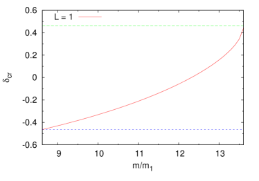
Figure 5: $\delta_{cr}$.

References

- Jag et al. (2016) M. Jag, M. Cetina, R. S. Lous, R. Grimm, J. Levinsen, and D. S. Petrov, Phys. Rev. A 94, 062706 (2016).
- Ospelkaus et al. (2006) C. Ospelkaus, S. Ospelkaus, K. Sengstock, and K. Bongs, Phys. Rev. Lett. 96, 020401 (2006).
- Fratini and Pieri (2012) E. Fratini and P. Pieri, Phys. Rev. A 85, 063618 (2012).
- Iskin and Sá de Melo (2006) M. Iskin and C. A. R. Sá de Melo, Phys. Rev. Lett. 97, 100404 (2006).
- Levinsen et al. (2009) J. Levinsen, T. G. Tiecke, J. T. M. Walraven, and D. S. Petrov, Phys. Rev. Lett. 103, 153202 (2009).
- Mathy et al. (2011) C. J. M. Mathy, M. M. Parish, and D. A. Huse, Phys. Rev. Lett. 106, 166404 (2011).
- Alzetto et al. (2012) F. Alzetto, R. Combescot, and X. Leyronas, Phys. Rev. A 86, 062708 (2012).
- Jag et al. (2014) M. Jag, M. Zaccanti, M. Cetina, R. S. Lous, F. Schreck, R. Grimm, D. S. Petrov, and J. Levinsen, Phys. Rev. Lett. 112, 075302 (2014).
- Kartavtsev and Malykh (2007a) O. I. Kartavtsev and A. V. Malykh, J. Phys. B 40, 1429 (2007a).
- Petrov (2003) D. S. Petrov, Phys. Rev. A 67, 010703(R) (2003).
- Kartavtsev and Malykh (2016) O. I. Kartavtsev and A. V. Malykh, EPL (Europhysics Letters) 115, 36005 (2016).
- Efimov (1973) V. Efimov, Nucl. Phys. A 210, 157 (1973).
- Nishida et al. (2008) Y. Nishida, D. T. Son, and S. Tan, Phys. Rev. Lett. 100, 090405 (2008).
- Safavi-Naini et al. (2013) A. Safavi-Naini, S. T. Rittenhouse, D. Blume, and H. R. Sadeghpour, Phys. Rev. A 87, 032713 (2013).
- Kartavtsev and Malykh (2014) O. I. Kartavtsev and A. V. Malykh, Phys. At. Nucl. 77, 430 (2014), [Yad. Fiz. 77, 458 (2014)].
- Minlos (2011a) R. A. Minlos, Mosc. Math. J. 11, 113 (2011a), Mosc. Math. J. 11, 815 (2011).
- Minlos (2012) R. A. Minlos, ISRN Math. Phys. 2012, 230245 (2012).
- Minlos (2014a) R. A. Minlos, Usp. Mat. Nauk 69(3), 145 (2014a), [Russ. Math. Surv. 69(3), 539 (2014)].
- Minlos (2014b) R. A. Minlos, Mosc. Math. J. 14, 617 (2014b).
- Correggi et al. (2012) M. Correggi, G. Dell’antonio, D. Finco, A. Michelangeli, and A. Teta, Rev. Math. Phys. 24, 1250017 (2012).
- Correggi et al. (2015a) M. Correggi, G. Dell’antonio, D. Finco, A. Michelangeli, and A. Teta, Math. Phys. Analys. Geom. 18, 32 (2015a).
- Correggi et al. (2015b) M. Correggi, D. Finco, and A. Teta, EPL 111, 10003 (2015b).
- Kartavtsev and Malykh (2007b) O. I. Kartavtsev and A. V. Malykh, Pis’ma ZhETF 86, 713 (2007b), [JETP Lett. 86, 625 (2007)].
- Endo et al. (2011) S. Endo, P. Naidon, and M. Ueda, Few-Body Syst. 51, 207 (2011).
- Helfrich and Hammer (2011) K. Helfrich and H.-W. Hammer, J. Phys. B 44, 215301 (2011).
- Macek (1968) J. H. Macek, J. Phys. B 1, 831 (1968).
- Kartavtsev (1999) O. I. Kartavtsev, Few-Body Syst. Suppl. 10, 199 (1999).
- Kartavtsev and Malykh (2006) O. I. Kartavtsev and A. V. Malykh, Phys. Rev. A 74, 042506 (2006).
- Minlos (2011b) R. A. Minlos, Mosc. Math. J. 11, 113 (2011b).
- Michelangeli and Ottolini (2018) A. Michelangeli and A. Ottolini, Reports on Mathematical Physics 81, 1 (2018).
- Becker et al. (2018) S. Becker, A. Michelangeli, and A. Ottolini, Mathematical Physics, Analysis and Geometry 21, 35 (2018).
- Castin and Tignone (2011) Y. Castin and E. Tignone, Phys. Rev. A 84, 062704 (2011).
- Case (1950) K. M. Case, Phys. Rev. 80, 797 (1950).
- Yakovlev and Gradusov (2013) S. L. Yakovlev and V. A. Gradusov, J. Phys. A 46, 035307 (2013).
- Albeverio et al. (1983) S. Albeverio, F. Gesztesy, R. Høegh-Krohn, and L. Streit, Annales de l’I. H. P., Section A 38, 263 (1983).
- Gao et al. (2015) C. Gao, S. Endo, and Y. Castin, Europhys. Lett. 109, 16003 (2015).
- Michelangeli and Schmidbauer (2013) A. Michelangeli and C. Schmidbauer, Phys. Rev. A 87, 053601 (2013).
- Nishida and Tan (2008) Y. Nishida and S. Tan, Phys. Rev. Lett. 101, 170401 (2008).
- Nishida and Tan (2011) Y. Nishida and S. Tan, Few-Body Syst. 51, 191 (2011).
- Lamporesi et al. (2010) G. Lamporesi, J. Catani, G. Barontini, Y. Nishida, M. Inguscio, and F. Minardi, Phys. Rev. Lett. 104, 153202 (2010).
- Shi et al. (2014) Z.-Y. Shi, X. Cui, and H. Zhai, Phys. Rev. Lett. 112, 013201 (2014).
- Cui and Yi (2014) X. Cui and W. Yi, Phys. Rev. X 4, 031026 (2014).
- Shi et al. (2015) Z.-Y. Shi, H. Zhai, and X. Cui, Phys. Rev. A 91, 023618 (2015).
- Castin et al. (2010) Y. Castin, C. Mora, and L. Pricoupenko, Phys. Rev. Lett. 105, 223201 (2010).
- Endo and Castin (2015) S. Endo and Y. Castin, Phys. Rev. A 92, 053624 (2015).
- Moser and Seiringer (2017) T. Moser and R. Seiringer, Comm. in Math. Phys. 356, 329 (2017).
- Bazak and Petrov (2017) B. Bazak and D. S. Petrov, Phys. Rev. Lett 118, 083002 (2017).
- Bazak (2017) B. Bazak, Phys. Rev. A 96, 022708 (2017).
- Moser and Seiringer (2018) T. Moser and R. Seiringer, Math. Phys., Anal. Geom. 21, 19 (2018).
- Michelangeli and Pfeiffer (2016) A. Michelangeli and P. Pfeiffer, J. Phys. A 49, 105301 (2016).
- Endo et al. (2012) S. Endo, P. Naidon, and M. Ueda, Phys. Rev. A 86, 062703 (2012).
- Bateman and Erdélyi (1953) H. Bateman and A. Erdélyi, Higher transcendental functions (Mc Graw-Hill, New York - Toronto - London, 1953).
- Gasaneo and Macek (2002) G. Gasaneo and J. H. Macek, J. Phys. B 35, 2239 (2002).
- Pade (2007) J. Pade, Eur. Phys. J. D 44, 345 (2007).
- Pade (2009) J. Pade, Eur. Phys. J. D 53, 41 (2009).
- Szmytkowski (1995) R. Szmytkowski, J. Phys. A 28, 7333 (1995).
- Gómez and Sesmaa (2012) F. J. Gómez and J. Sesmaa, Eur. Phys. J. D 66, 6 (2012).
- Gao (2003) B. Gao, J. Phys. B 36, 2111 (2003).
- Bouaziz and Bawin (2014) D. Bouaziz and M. Bawin, Phys. Rev. A 89, 022113 (2014).
- Moroz et al. (2015) S. Moroz, J. P. D’Incao, and D. S. Petrov, Phys. Rev. Lett. 115, 180406 (2015).
- Braaten and Phillips (2004) E. Braaten and D. Phillips, Phys. Rev. A 70, 052111 (2004).