A multiscale model for Rayleigh-Taylor and Richtmyer-Meshkov instabilities

Abstract

We develop a novel multiscale model of interface motion for the Rayleigh-Taylor instability (RTI) and Richtmyer-Meshkov instability (RMI) for two-dimensional, inviscid, compressible flows with vorticity, which yields a fast-running numerical algorithm that produces both qualitatively and quantitatively similar results to a resolved gas dynamics code, while running approximately two orders of magnitude (in time) faster. Our multiscale model is founded upon a new compressible-incompressible decomposition of the velocity field $u=v+w$. The incompressible component $w$ of the velocity is also irrotational and is solved using a new asymptotic model of the Birkhoff-Rott singular integral formulation of the incompressible Euler equations, which reduces the problem to one spatial dimension. This asymptotic model, called the higher-order $z$-model, is derived using small nonlocality as the asymptotic parameter, allows for interface turn-over and roll-up, and yields a significant simplification for the equation describing the evolution of the amplitude of vorticity. This incompressible component $w$ of the velocity controls the small scale structures of the interface and can be solved efficiently on fine grids. Meanwhile, the compressible component of the velocity $v$ remains continuous near contact discontinuities and can be computed on relatively coarse grids, while receiving subgrid scale information from $w$. We first validate the incompressible higher-order $z$-model by comparison with classical RTI experiments as well as full point vortex simulations. We then consider both the RTI and the RMI problems for our multiscale model of compressible flow with vorticity, and show excellent agreement with our high-resolution gas dynamics solutions.

1.  Introduction

The instability that occurs when an interface separating two fluids of different densities is perturbed and subjected to an acceleration force is a fundamental problem in fluid mechanics. The Rayleigh-Taylor instability (RTI) [67, 96] occurs when the lighter fluid is accelerated towards the heavier fluid (under the action of gravity, for instance). The Richtmyer-Meshkov instability (RMI) [81, 71] is initiated by the passage of a shock wave across the perturbed interface separating the two fluids. In either case, perturbations of the interface initially grow according to the linear theory, before the system enters the nonlinear regime, in which the light fluid bubbles into the heavy fluid, while the heavy fluid spikes into the light fluid. The velocity of the resulting flow is discontinuous at the material interface (or contact discontintuity), which initiates the Kelvin-Helmholtz instability (KHI) [89, 50]. This causes the interface to roll up into complex vortical structures, and eventually leads to turbulent mixing. Each of these instabilities arises in numerous important applications, including in astrophysics [51], inertial confinement fusion [13], and ocean mixing [90]. We refer the reader to the works [85, 58, 15] and the references therein for further details.

The fundamental mathematical model for the RT and RM instabilities is the Euler system of hydrodynamics equations, consisting of the conservation of mass, momentum, and energy. The mathematical analysis of the Euler equations is extremely challenging due to the ill-posed nature of the equations in the absence of of stabilizing mechanisms such as surface tension or viscosity, with the RTI and RMI causing growth of perturbations at the smallest scales available. The highly unstable nature of both the RTI and RMI also poses significant difficulties for numerical methods, and the development of algorithms to study these instabilities has been the subject of intensive research over the last several decades [32, 9, 40, 98, 41, 36, 1, 59], and continues to remain a challenge.

As the linear theory shows, the highest frequency perturbations of the interface have the largest growth rates; numerical solutions thus often suffer from the development of spurious small scale structure [62], which does not appear to agree with laboratory experiments [104]. Numerical methods with a large amount of implicit diffusion suppress these small scale eddies, but, in doing so, prevent the development of the KHI mixing zones.

Moreover, even when numerical schemes can be manipulated into producing better solutions [78], simulations can be prohibitively (computationally) expensive. Direct Numerical Simulations (DNS) solve the complete governing equations with exact physical parameters and sufficient resolution to represent all the scales of the flow [73], but the requirement that all the spatial and temporal scales be numerically resolved results in overwhelmingly expensive calculations, both in terms of computational runtime, as well as other basic computational resources, such as memory. As such, simulations are currently generally limited to small Reynolds number flows and simple geometries [102]. These observations indicate a great need for fast algorithms that can be used to accurately predict the RTI and RMI mixing layers and associated growth rates.

In this work, we develop a multiscale model for interface evolution during RTI and RMI for two-dimensional, inviscid, compressible flow with vorticity. Our multiscale model is founded upon a new compressible-incompressible decomposition of the velocity field $u=v+w$, which is, in turn, based upon a two-phase elliptic system of Hodge type [19]. The incompressible component $w$ of the velocity is also irrotational and is solved using a new asymptotic model of the Birkhoff-Rott singular-integral formulation of the incompressible Euler equations, which already reduces the problem to one spatial dimension. This asymptotic model, called the higher-order $z$-model, is derived using small nonlocality as the asymptotic parameter, allows for interface turn-over and roll up, and yields a significant simplification for the equation describing the evolution of the amplitude of vorticity. This incompressible component $w$ of the velocity controls the small scale structures of the interface and can be solved efficiently on fine grids. Meanwhile, the compressible component of the velocity $v$ field remains smooth near contact discontinuities and can be computed on relatively coarse grids, while receiving subgrid scale information from $w$.

Specifically, our higher-order $z$-model, approximates the Birkhoff-Rott (BR) equations [26] of interface evolution in two-dimensional multiphase incompressible and irrotational flow, which are, in turn, a reduction of the incompressible and irrotational Euler equation to one-dimensional evolution for the parameterization of the interface $z(\alpha,t)=\left(z_{1}(\alpha,t),z_{2}(\alpha,t)\right)$ and the amplitude of vorticity $\varpi(\alpha,t)$. The original (low-order) $z$-model was derived by Granero-Belinchón and Shkoller [44] using an asymptotic expansion in a small non-locality parameter, and its main advantage over the full BR evolution is a drastic simplification of the dynamics for the amplitude of vorticity $\varpi$. Without this simplification, the BR dynamics of $\varpi$ is nonlinear, non-local, and is in fact a Fredholm integro-differential equation of the second kind. Numerical methods for this type of equation are thus often quite complex and computationally expensive. On the other hand, the $\varpi$ dynamics given by the $z$-model allow us to implement an extremely simple numerical method which avoids costly upwinding and iterative procedures [7, 92]; in particular, we use a simple Fourier collocation method to evolve $\varpi$. For the evolution of the interface $z$, the original (low-order) $z$-model of [44] used a local equation, while our new (high-order) $z$-model instead uses Krasny’s $\delta$-desingularization [56] of the singular integral kernel. The solution of $z$ and $\varpi$ then provide us with the incompressible velocity field $w$ via an efficient kernel computation. The compressible velocity field $v$ is solved on a very coarse grid (while receiving small-scale information from $w$) using a very simple WENO scheme together with a nonlinear, spacetime smooth, artificial viscosity method termed the $C$-method [80, 77, 78].

We first validate our incompressible and irrotational (high-order) $z$-model by performing a number of numerical experiments, including both the single-mode and multi-mode RTI, to demonstrate the accuracy of the $z$-model and its numerical implementation. The computed $z$-model solutions are compared with observations from laboratory experiments [104, 79, 107], and are shown to achieve very similar growth rates of the bubbles and spikes, as well as the mixing layer. We additionally compare our $z$-model solutions with “reference” solutions computed using a sophisticated numerical method for the complete Birkhoff-Rott equations [92], and show that the two solutions are in excellent agreement, thereby demonstrating the validity of the $z$-model. Moreover, our simplified model equations allow for a numerical computation that is a factor of at least 75 times faster than the reference solution calculation. We also compare the simple Krasny desingularization used in the numerical implementation of the $z$-model with two other higher-order regularizations that smooth the singular integral kernel via convolution with Gaussian-type functions which satisfy certain moment conditions. We demonstrate that all three numerical methods for smoothing the singular integral produce similar numerical solutions (in a sense to be made precise below); as will be shown, these solutions are in reasonable agreement in the asymptotic limit as the mesh spacing ${\scriptstyle\Delta}\alpha$ and viscosity parameter $\delta$ converge to zero.

Then, we use our multiscale model, designed to simulate interface evolution in compressible flows with vorticity. As we noted above, we decompose $u=v+w$, where $w$ is both divergence-free and curl-free, but has a discontinuity in its tangential component across the contact discontinuity, while $v$ is continuous across the contact, but is forced by the bulk compression and vorticity of the fluid. By analogy with turbulence models, such as large-eddy simulation (LES) [70], Reynolds-averaged Navier-Stokes (RANS), and Lagrangian-averaged Navier-Stokes (LANS-$\alpha$) [72], our multiscale model involves the decomposition of the flow into a part which can be solved on a coarse grid (the mean flow), and a part which must be solved on a fine grid (the sub-grid scale fluctuations). The novelty of our approach is that, for the RTI and RMI, the fine grid coincides with the interface itself, and is thus one-dimensional. This means that fine structures can be simulated with much less computational expense than is required for fully two-dimensional calculations on similarly fine meshes.

We describe a simple Eulerian-Lagrangian algorithm for our multiscale model that couples the equations on a coarse two-dimensional mesh with the equations on the high resolution one-dimensional interface. For modeling the RMI, a modified set of equations is used, in which we account for both the effects of shock-contact interaction, as well as the classical Taylor “frozen turbulence” hypothesis [95]. We then discuss the numerical implementation of the algorithm, which uses our incompressible $z$-model, as well as simple interpolation and integral-kernel calculation techniques. A number of numerical experiments for the RTI and RMI are performed to demonstrate the efficacy of our multiscale model and algorithm for compressible flows with vorticity. In particular, we show that our algorithm produces solutions that agree both qualitatively and quantitatively with (relatively) high-resolution reference solutions. We again perform some basic convergence studies, and find good agreement between the multiscale solutions and high-resolution reference solutions in the limit as the interfacial mesh spacing ${\scriptstyle\Delta}\alpha$ and desingularization parameter $\delta$ converge to zero. Moreover, the run times of our multiscale algorithm are two orders of magnitude (or more) faster than those of the corresponding high-resolution reference solutions.

Outline of the paper. Section 2 is devoted to the notation and definitions that will be used throughout the paper. In Section 3, we introduce the full system of Euler equations for compressible flow, followed by the incompressible and irrotational simplification. For the latter, we explain how those equations can be solved using the Birkhoff-Rott singular integral-kernel equations for the interface parameterization and amplitude of vorticity. We then describe our asymptotic (in nonlocality) $z$-model. We next consider the full compressible Euler equations as a two-phase elliptic system for the velocity, and derive a novel compressible-incompressible decomposition of the velocity. This decomposition is the foundation of our multiscale model and algorithm.

In Section 4, we consider the numerical implementation of the incompressible $z$-model. A simple numerical method is introduced, and results for several numerical experiments are shown, including comparisons with laboratory experiments, theoretical predictions and models, and benchmark numerical simulations. We then present, in Section 5, our multiscale model and algorithms for the compressible RTI and RMI, and give details about their numerical implementations.

Our multiscale algorithm is then applied to two RTI and two RMI test problems Section 6, and compared against both high-resolution simulations and low-resolution simulations. Finally, our conclusions are in Section 7. Two short sections of the Appendix are provided: the first concerns mesh refinement studies for the multiscale algorithm and the second summarizes our numerical method for gas dynamics.

2.  Preliminaries

2.1.  Some notation and definitions

2.1.1.  Derivatives

We write

$$\partial_{i}f=\frac{\partial f}{\partial x_{i}}\ \text{ for }i=1,2\,,\ \ \partial_{t}f=\frac{\partial f}{\partial t}\,,\ \ \nabla=(\partial_{\!1},\partial_{2})\,,\ \ \nabla^{\perp}=(-\partial_{2},\partial_{\!1})\,,$$

and for a vector $F$,

$$\operatorname{div}F=\nabla\cdot F\ \text{ and }\ \operatorname{curl}F=\nabla^{\perp}\cdot F\,.$$

The Laplace operator is defined as $\Delta=\partial_{\!1}^{2}+\partial_{2}^{2}$. Given a transport velocity $u(x,t)$, we shall denote the material derivative $\partial_{t}+u\cdot\nabla$ by $\tfrac{\mathrm{D}}{\mathrm{D}t}$.

2.1.2.  Fourier series

Let $\mathbb{T}_{L}$ denote the interval $[-L/2,L/2]$. If $f:\mathbb{T}_{L}\to\mathbb{R}$ is a square-integrable $L$-periodic function, then it has the Fourier series representation $f(\alpha)=\sum\limits_{k=-\infty}^{\infty}{\widehat{f}}(k)e^{\frac{2\pi ik\alpha}{L}}$ for all $\alpha\in\mathbb{T}_{L}$, where the complex Fourier coefficients are defined by $\mathcal{F}\{f\}(k)\equiv{\widehat{f}}(k)={\dfrac{1}{L}}\int_{\mathbb{T}_{L}}{}\,f(\alpha)e^{-\frac{2\pi ik\alpha}{L}}\,\mathrm{d}\alpha$. We have the following standard identity:

$$\mathcal{F}\{\partial^{n}_{\alpha}f\}(k)=\left(\frac{2i\pi}{L}k\right)^{n}{\widehat{f}}(k)\,,$$ (1)

where $\partial_{\alpha}=\frac{\partial}{\partial\alpha}$. We shall sometimes write ${\widehat{f}}_{k}$ for ${\widehat{f}}(k)$.

2.1.3.  Principal value integral

The principal value integral of a function $f:\mathbb{R}\to\mathbb{R}$ is defined as

$$\operatorname{P}\int_{\mathbb{R}}f(\beta)\,\mathrm{d}\beta\coloneqq\lim_{\varepsilon\to 0^{+}}\int_{(-1/\varepsilon,-\varepsilon)\cup(\varepsilon,1/\varepsilon)}f(\beta)\,\mathrm{d}\beta\,.$$ (2)

2.1.4.  Hilbert transform

The Hilbert transform of a function $f:\mathbb{R}\to\mathbb{R}$ is defined as

$$\mathcal{H}f(\alpha)=\frac{1}{\pi}\operatorname{P}\int_{\mathbb{R}}\frac{f(\beta)}{\alpha-\beta}\,\mathrm{d}\beta\,.$$ (3)

If $f$ is an $L$-periodic function on $\mathbb{T}_{L}$, then

$$\mathcal{H}f(\alpha)=\frac{1}{L}\operatorname{P}\int_{\mathbb{T}_{L}}\frac{f(\beta)}{\tan(\tfrac{\pi}{L}(\alpha-\beta))}\,\mathrm{d}\beta\,.$$ (4)

Equivalently, using the Fourier representation, the Hilbert transform $\mathcal{H}$ can be defined as

$${\widehat{\mathcal{H}f}}(k)=-i\text{sgn}(k){\widehat{f}}(k)\,.$$ (5)

In particular, we note that $\mathcal{H}^{2}=-1$.

2.1.5.  Discrete operators in Fourier space

Let $\alpha\in\mathbb{T}_{L}$. We discretize the parameter $\alpha$ with $N+1=2^{r}+1$ nodes,

$$\alpha_{k}=-L/2+(k-1){\scriptstyle\Delta}\alpha\,,$$

with ${\scriptstyle\Delta}\alpha=L/N$. Given an $L$-periodic function $f(\alpha)$, we denote by $f_{k}=f(\alpha_{k})$ the function $f$ evaluated at a point $\alpha_{k}\in\mathbb{T}_{L}$ Let $\tilde{\mathcal{F}}$ and $\tilde{\mathcal{F}}^{-1}$ denote the discrete Fourier and inverse Fourier transforms, respectively, defined for sequences $(f_{k})$ of length $N=2^{r}$ by

$$\tilde{\mathcal{F}}\left\{f_{k}\right\}_{m}=\sum_{l=1}^{N}f_{l}\cdot e^{-\frac{2i\pi}{N}(m-1)(l-1)}\quad\text{ and }\quad\tilde{\mathcal{F}}^{-1}\left\{{\widehat{f}}_{m}\right\}_{k}=\frac{1}{N}\sum_{l=1}^{N}{\widehat{f}}_{l}\cdot e^{\frac{2i\pi}{N}(k-1)(l-1)}\,.$$

We define the discrete Fourier operators $(H_{k})$, $(D_{k})$, $(D^{2}_{k})\in\mathbb{C}^{N}$ as

$$H_{k} =\begin{cases}0&\text{if }k=1\,,\\ -i&\text{if }2\leq k\leq(N+1)/2\,,\\ i&\text{if }k>(N+1)/2\,,\end{cases}$$ (6)

$$D_{k} =\begin{cases}\frac{2\pi i}{L}(k-1)&\text{if }k<(N+1)/2\,,\\ 0&\text{if }k=(N+1)/2\,,\\ -\frac{2\pi i}{L}(N-k)&\text{if }k>(N+1)/2\,,\end{cases}$$ (7)

$$D^{2}_{k} =\begin{cases}-\left(\frac{2\pi}{L}\right)^{2}(k-1)^{2}&\text{if }k\leq(N+1)/2\,,\\ -\left(\frac{2\pi}{L}\right)^{2}(N-k)^{2}&\text{if }k>(N+1)/2\,.\end{cases}$$ (8)

Formula (6) is the discrete Hilbert transform in Fourier space, while (7) and (8) are the discrete derivative operators $\partial_{\alpha}$ and $\partial^{2}_{\alpha}$, respectively, in Fourier space.

2.2.  Computational platform and code optimization

All of the numerical simulations conducted in this work were run on a Macbook Pro laptop using a 2.4 GHz Intel Core i5 processor with 8 GB of RAM. The operating system is macOS High Sierra 10.13.6, and the GFortran F90 compiler is used.

The codes for the numerical methods described in the paper are implemented in the same programming framework, but are not otherwise specially optimized (apart from a specific calculation described in the paper). The same input, output, and timing routines are used in all of the codes. This consistency allows for a reliable comparison of the different algorithms and their associated imposed computational burden.

3.  The Euler equations

3.1.  The compressible Euler equations

The fundamental mathematical model for the motion of an inviscid two-dimensional fluid is given by the compressible Euler equations:

$$\partial_{t}\rho+\operatorname{div}(\rho u) =0\,,$$ (9a)

$$\partial_{t}(\rho u)+\operatorname{div}(\rho u\otimes u)+\nabla p+\rho ge_{2} =0\,,$$ (9b)

$$\partial_{t}E+\operatorname{div}(u(E+p))+\rho gu_{2} =0\,,$$ (9c)

where $\otimes$ denotes the tensor product, and $\operatorname{div}M$ denotes the row-wise divergence of a matrix $M$. The velocity vector is ${u}=(u_{1}\,,u_{2})$ with horizontal component $u_{1}$ and vertical component $u_{2}$, $\rho>0$ is the fluid density (assumed strictly positive), $E$ denotes the energy, and $p$ is the pressure defined by an equation of state. These equations are, in fact, the basic conservation laws of fluid dynamics: (9a) is conservation of mass, (9b) is conservation of linear momentum, and (9c) is conservation of energy.

The system (9) can be written in classical conservation-law form as the Cauchy problem

$$\partial_{t}{\bf{U}}(x,t)+\partial_{x_{1}}{\bf{F}}({\bf{U}}(x,t))+\partial_{x_{2}}{\bf{G}}({\bf{U}}(x,t))={\bf H}(x,t), \ \ \ {x}\in\mathbb{R}^{2}\,,t>0,$$ (10a)

$${\bf{U}}(x,0)={\bf{U}}_{0}({x}), \ \ \ {x}\in\mathbb{R}^{2}\,,t=0,$$ (10b)

where the 4-vector $\bf{U}$ and the flux functions ${\bf{F}}({\bf{U}})$ and ${\bf{G}}({\bf{U}})$ are defined as

$${\bf U}=\left(\begin{array}[]{c}\rho\\ \rho u_{1}\\ \rho u_{2}\\ E\end{array}\right)\quad\text{ and }\quad{\bf F}({\bf U})=\begin{pmatrix}\rho u_{1}\\ \rho u_{1}^{2}+p\\ \rho u_{1}u_{2}\\ u_{1}(E+p)\end{pmatrix}\,\quad\text{ and }\quad\bf{G}(\bf{U})=\begin{pmatrix}\rho u_{2}\\ \rho u_{1}u_{2}\\ \rho u_{2}^{2}+p\\ u_{2}(E+p)\end{pmatrix}\,.$$ (11)

The space coordinate is $x=(x_{1},x_{2})$, with $x_{1}$ denoting the horizontal component, $x_{2}$ denoting the vertical component, and $t\geq 0$ denoting time. The function $\bf H$ denotes the forcing function due to gravity, and so will be given as ${\bf H}=(0\,,0\,,-\rho g\,,-\rho gu_{2})$, where $g$ is a gravitational acceleration constant. The pressure $p$ is defined by the ideal gas law,

$$p=(\gamma-1)\left(E-\frac{1}{2}\rho|{u}|^{2}\right)\,,$$ (12)

where $\gamma$ is the adiabatic constant, which we will assume takes the value $\gamma=1.4$, unless otherwise stated. We also define the specific internal energy per unit mass of the fluid as $e=p/(\rho(\gamma-1))$. Once the initial data $u_{0}(x)$, $\rho_{0}(x)$, $E_{0}(x)$ are specified, solutions of (10) provide the velocity, density, and energy for each instant of time for which the solution exits.

3.2.  The incompressible and irrotational Euler equations

In the absence of sound waves, the system (9) can be simplified to model incompressible flows. The incompressible Euler equations are written as

$$\rho\left[\partial_{t}{w}(x,t)+(w\cdot\nabla)w\right]+\nabla p+g\rho e_{2}=0, \ \ \ {x}\in\mathbb{R}^{2}\,,t>0,$$ (13a)

$$\operatorname{div}w=0, \ \ \ {x}\in\mathbb{R}^{2}\,,t\geq 0,$$ (13b)

$${w}(x,0)={w}_{0}({x}), \ \ \ {x}\in\mathbb{R}^{2}\,,t=0\,,$$ (13c)

where $w=(w_{1},w_{2})$ denotes a divergence-free velocity vector field, the density $\rho$ is assumed to be a constant (or piecewise constant as we shall consider below), and the pressure $p$ is a Lagrange multiplier which enforces the incompressibility constraint (13b). We define the two-dimensional vorticity function $\omega=\operatorname{curl}w$, where

$$\operatorname{curl}w:=\nabla^{\perp}\cdot w=\partial_{1}w_{2}-\partial_{2}w_{1}\,.$$

Computing the $\operatorname{curl}$ of (13a) and using (13b) shows that the two-dimensional vorticity is transported by incompressible flows,

$$\partial_{t}\omega+w\cdot\nabla\omega=0\,,$$

and hence if the initial velocity $w_{0}(x)$ is chosen to be irrotational such that $\omega_{0}(x)=0$, then $\omega(x,t)=0$ for all time $t$ for which the solution exists. Thus, for such data, we supplement (13) with

$$\operatorname{curl}w=0, \ \ \ {x}\in\mathbb{R}^{2}\,,t\geq 0\,.$$ (13d)

3.3.  The compressible Euler equations as a two-phase hyperbolic system

We are particularly interested in two-dimensional discontinuous solutions of the Euler equations (10) which propagate curves of discontinuity, whose evolution is determined by the Rankine-Hugoniot conditions (see, for example, [31]). Specifically, our focus is on two-dimensional solutions ${\bf U}=(\rho,\rho u_{1},\rho u_{2},E)$ to (10) which have jump discontinuities across a time-dependent, space-periodic material interface $\Gamma(t)$ (see Figure 1).

Figure 1: An example of a time-dependent contact discontinuity $\Gamma(t)$ separating the two fluid regions $\Omega^{+}(t)$ and $\Omega^{-}(t)$.

The two-dimensional fluid domain is written as

$$\mathbb{R}^{2}=\Omega^{+}(t)\cup\Omega^{-}(t)\cup\Gamma(t)\,,$$

where $\Omega^{+}(t)$ denotes the time-dependent open domain lying above $\Gamma(t)$, while $\Omega^{-}(t)$ denotes the open domain lying below $\Gamma(t)$. We let $n(\cdot,t)$ denote the unit normal vector to $\Gamma(t)$ pointing into $\Omega^{+}(t)$ and let $\tau(\cdot,t)$ denote the unit tangent vector to $\Gamma(t)$, so that the pair $(\tau,n)$ denote a right-handed basis. We denote by ${\bf{U}}^{+}$ the solution in the domain $\Omega^{+}(t)$ and by ${\bf U}^{-}$, the solution in $\Omega^{-}(t)$. The jump of a function ${\bf{U}}$ across $\Gamma(t)$ is denoted by

$$\llbracket{\bf{U}}\rrbracket={\bf{U}}^{+}-{\bf{U}}^{-}\text{ on }\Gamma(t)\,.$$

The Rankine-Hugoniot conditions relate the speed of propagation ${\sigma}(t)$ of the curve of discontinuity $\Gamma(t)$ with the jump discontinuity in the variables ${\bf U}=(\rho,\rho u_{1},\rho u_{2},E)$ via the relation

$${\sigma}\llbracket{\rho}\rrbracket =\llbracket\rho u\cdot n\rrbracket\,,$$ (14a)

$${\sigma}\llbracket{\rho u}\rrbracket =\llbracket(\rho u\cdot n)u+pn\rrbracket\,,$$ (14b)

$${\sigma}\llbracket{E}\rrbracket =\llbracket(E+p)u\cdot n\rrbracket\,,$$ (14c)

which represent, respectively, the conservation of mass, linear momentum, and energy across the discontinuity. Notice that (14b) admits solutions with $\llbracket p\rrbracket=0$ and $\llbracket(\sigma-u\cdot n)\rho u\rrbracket=0$, and that the latter condition is satisfied if $u^{\pm}\cdot n=\sigma$. Such discontinuities are known as contact discontinuities, in which case the interface $\Gamma(t)$ is transported by the fluid velocity $u$, and the pressure $p$ is continuous across $\Gamma(t)$. Contact discontinuities are the class of two-dimensional discontinuous solutions solving the following coupled two-phase system of hyperbolic equations:

$$\partial_{t}\rho^{\pm}+\operatorname{div}(\rho u^{\pm}) =0,\qquad \text{ in }\Omega^{\pm}(t)\,,$$ (15a)

$$\partial_{t}(\rho^{\pm}u^{\pm})+\operatorname{div}(\rho^{\pm}u^{\pm}\otimes u^{\pm})+\nabla p^{\pm}+\rho ge_{2} =0,\qquad \text{ in }\Omega^{\pm}(t)\,,$$ (15b)

$$\partial_{t}E^{\pm}+\operatorname{div}(u^{\pm}(E^{\pm}+p^{\pm}))+\rho gu^{\pm}_{2} =0,\qquad \text{ in }\Omega^{\pm}(t)\,,$$ (15c)

$$\llbracket{u}\cdot n\rrbracket =0,\qquad \text{ on }\Gamma(t)\,,$$ (15d)

$$\llbracket{u}\cdot\tau\rrbracket \neq 0,\qquad \text{ on }\Gamma(t)\,,$$ (15e)

$$\llbracket p\rrbracket =0,\qquad \text{ on }\Gamma(t)\,,$$ (15f)

$$\left(u^{\pm}(x,0),\rho^{\pm}(x,0),E^{\pm}(x,0),\Gamma(0)\right) =\left(u^{\pm}_{0},\rho^{\pm}_{0},E^{\pm}_{0},\Gamma_{0}\right),\qquad \text{ at }t=0\,.$$ (15g)

As already noted the interface $\Gamma(t)$ is transported by the velocity $u$ and we will make the dynamics of $\Gamma(t)$ precise, once we introduce a parameterization for $\Gamma(t)$. The tangential velocity jump discontinuity is the primary mechanism that initiates the Kelvin-Helmholtz instability . The densities $\rho^{\pm}$ and the energies $E^{\pm}$ are, in general, also discontinuous across $\Gamma(t)$. The initial data is specified in (15g).

3.4.  The two-phase incompressible and irrotational Euler equations

The incompressible and irrotational Euler equations for two-phase flow are written as

$$\rho^{\pm}\left(\partial_{t}{w}^{\pm}+{w}^{\pm}\cdot\nabla{w}^{\pm}\right)+\nabla p^{\pm}+\rho^{\pm}ge_{2} =0\qquad \text{ in }\Omega^{\pm}(t)\,,$$ (16a)

$$\operatorname{curl}w=\operatorname{div}w =0\qquad \text{ in }\Omega^{\pm}(t)\,,$$ (16b)

$$\llbracket{w}\cdot n\rrbracket =0\qquad \text{ on }\Gamma(t)\,,$$ (16c)

$$\llbracket{w}\cdot\tau\rrbracket \neq 0\qquad \text{ on }\Gamma(t)\,,$$ (16d)

$$\llbracket p\rrbracket =0\qquad \text{ on }\Gamma(t)\,,$$ (16e)

$$\left(w^{\pm}(x,0),\Gamma(0)\right) =\left(w^{\pm}_{0},\Gamma_{0}\right)\qquad \text{ at }t=0\,,$$ (16f)

and $\rho^{+}$ and $\rho^{-}$ are constant in each phase. Again, the interface $\Gamma(t)$ is transported by the velocity $w$, and for incompressible and irrotational flows, the interface $\Gamma(t)$ is called a vortex sheet, because the vorticity is restricted to the one-dimensional interface as a measure, as will be made precise.

Incompressibility and irrotationality of the flow allow for a reduction of the system (16) to a coupled system of evolution equations in one space dimension. We let $\mathbb{T}_{L}=[-L/2\,,L/2]$ denote a (periodic) interval of length $L$, and introduce a parameterization of the interface $\Gamma(t)$ by a mapping $z:\mathbb{T}_{L}\to\mathbb{R}^{2}$, so that for each $\alpha$ in $\mathbb{T}_{L}$, the vector $z(\alpha,t)={\left(z_{1}(\alpha,t),z_{2}(\alpha,t)\right)}$ represents a point on the interface $\Gamma(t)$. Moreover, for any $\alpha_{0}$, the vector $\partial_{\alpha}z(\alpha_{0},t)$ is tangent to $\Gamma(t)$ at the point $z(\alpha_{0},t)$, and $\tau=\partial_{\alpha}z/|\partial_{\alpha}z|$ is the unit tangent vector at that point (as shown in Figure 2).

Figure 2: The curve $\Gamma(t)$ is parameterized by $z(\alpha,t)=(z_{1}(\alpha,t),z_{2}(\alpha,t))$. A tangent vector at a point $z(\alpha,t)$ on $\Gamma(t)$ is given by $\partial_{\alpha}z(\alpha,t)$.

Now, since $\Gamma(t)$ moves with speed $w\cdot n$, it follows that $\partial_{t}z(\alpha,t)=\left[w(z(\alpha,t),t)\cdot n\right]n$ and that the tangential motion of the interface $\partial_{t}z\cdot\partial_{\alpha}z$ has no constraints at all. The dynamics of the interface $\Gamma(t)$ are governed by the evolution equation

$$\partial_{t}z(\alpha,t)=w(z(\alpha,t),t)\,.$$ (17)

The vorticity $\omega$ vanishes in each of $\Omega^{\pm}(t)$, and is in fact a measure supported on $\Gamma(t)$, written as

$$\omega=\varpi\delta_{\Gamma(t)}\,,$$

where $\delta_{\Gamma(t)}$ is the Dirac delta distribution supported on $\Gamma(t)$, and the function $\varpi$ is the amplitude of vorticity along $\Gamma(t)$. More precisely, if $\varphi$ is any smooth test function with compact support in $\mathbb{R}^{2}$, then

$$\langle\omega\,,\varphi\rangle=\int_{\mathbb{R}}\varpi(\beta,t)\varphi(z(\beta,t))\,\mathrm{d}\beta\,.$$

The amplitude of vorticity $\varpi$ may be computed in terms of the jump in the velocity as

$$\begin{split}\int_{\mathbb{R}}\varpi(\beta,t)\varphi(z(\beta,t))\,\mathrm{d}\beta=\langle\omega\,,\varphi\rangle&\coloneqq-\int_{\Omega}w\cdot\nabla^{\perp}\varphi\,\mathrm{d}x\\ &=\int_{\Omega^{+}\cup\Omega^{-}}\varphi\nabla^{\perp}\cdot w\,\mathrm{d}x-\int_{\Gamma}\llbracket w\cdot\tau\rrbracket\varphi\,\mathrm{d}S\,.\end{split}$$

Since the vorticity $\omega=\nabla^{\perp}\cdot w=0$ in $\Omega^{+}(t)\cup\Omega^{-}(t)$, it then follows that

$$\int_{\mathbb{T}_{L}}\varpi(\beta,t)\varphi(z(\beta,t))\,\mathrm{d}\beta=-\int_{\Gamma}\llbracket w\cdot\tau\rrbracket\varphi\,\mathrm{d}S=-\int_{\mathbb{R}}\llbracket w\cdot\tau\rrbracket\varphi(z(\beta,t))|\partial_{\alpha}z(\beta,t)|\,\mathrm{d}\beta$$

for any smooth test function $\varphi$ with compact support in $\mathbb{R}^{2}$, which implies that

$$\varpi=-\llbracket w\cdot\tau\rrbracket|\partial_{\alpha}z|=-\llbracket w\cdot\partial_{\alpha}z\rrbracket\,.$$

Due to the fact that the flow is both irrotational and incompressible, there exist scalar stream functions $\psi^{\pm}(x,t)$ such that $\Delta\psi^{\pm}=0$ in $\Omega^{\pm}(t)$ and $w^{\pm}=\nabla^{\perp}\psi^{\pm}$.

Following [83, 14], we next reduce (16) to a system of coupled evolutionary integro-differential equations in one space dimension. The incompressible and irrotational velocity $w$ can be reconstructed from the vorticity measure $\varpi$ using the well-known Biot-Savart kernel $\mathcal{K}_{\mathbb{R}}(x)$, which is an integral representation for $\nabla^{\perp}\Delta^{-1}$ in $\mathbb{R}^{2}$. The kernel is defined by

$$\mathcal{K}_{\mathbb{R}}(x)=\frac{x^{\perp}}{2\pi|x|^{2}}=\frac{1}{2\pi}\left(\frac{-x_{2}}{x_{1}^{2}+x_{2}^{2}}\,,\frac{x_{1}}{x_{1}^{2}+x_{2}^{2}}\right)\,.$$ (18)

Away from the interface, the velocity $w$ is then given as

$$w(x,t)=\operatorname{P}\int_{\mathbb{R}}\mathcal{K}_{\mathbb{R}}(x-z(\beta,t))\varpi(\beta,t)\,\mathrm{d}\beta\,,$$ (19)

for $x\in\Omega^{+}(t)\cup\Omega^{-}(t)$, where we recall that the integral is to be understood in the principal value sense (2). At the interface $\Gamma(t)$, the velocity $w|_{\Gamma(t)}$ is defined to be the average $(w^{+}+w^{-})/2$ on $\Gamma(t)$. The Plemelj formulae give

$$w^{\pm}(z(\alpha,t),t)=\operatorname{P}\int_{\mathbb{R}}\mathcal{K}_{\mathbb{R}}(z(\alpha,t)-z(\beta,t))\varpi(\beta,t)\,\mathrm{d}\beta\pm\frac{1}{2}\frac{\varpi(\alpha,t)}{|\partial_{\alpha}z(\alpha,t)|}\tau\,,$$

from which it follows that

$$w(z(\alpha,t),t)=\operatorname{P}\int_{\mathbb{R}}\mathcal{K}_{\mathbb{R}}(z(\alpha,t)-z(\beta,t))\varpi(\beta,t)\,\mathrm{d}\beta\,.$$

This integral is over the real line. For horizontally periodic flows, the integral can be summed over the periodic images to yield an integral over a single period, with the kernel given by

$$\mathcal{K}_{\mathbb{T}_{L}}(x)=\frac{\left(-\sinh(2\pi x_{2}/L)\,,\sin(2\pi x_{1}/L)\right)}{2L\left(\cosh(2\pi x_{2}/L)-\cos(2\pi x_{1}/L)\right)}\,,$$ (20)

where $\mathbb{T}_{L}=[-L/2\,,L/2]$ denotes the periodic interval with period $L$. Hence,

$$w(z(\alpha,t),t)=\operatorname{P}\int_{\mathbb{T}_{L}}\mathcal{K}_{\mathbb{T}_{L}}(z(\alpha,t)-z(\beta,t))\varpi(\beta,t)\,\mathrm{d}\beta\,.$$ (21)

Together with (17), the system is closed by determining the evolution equation for the amplitude of vorticity $\varpi$. A lengthy computation [26, 44] using the Bernoulli equation, the Plemelj formulae, and (16e) provides the dynamics for $\varpi$; together with (17) and (21), we obtain the following coupled system:

$$\partial_{t}z(\alpha,t) =\operatorname{P}\int_{\mathbb{T}_{L}}\mathcal{K}_{\mathbb{T}_{L}}(z(\alpha,t)-z(\beta,t))\varpi(\beta,t)\,\mathrm{d}\beta\,,$$ (22a)

$$\partial_{t}\varpi(\alpha,t) =-\partial_{\alpha}\left[\frac{A}{4\pi^{2}}\left|\operatorname{P}\int_{\mathbb{R}}\varpi(\beta,t)\frac{(z(\alpha,t)-z(\beta,t))^{\perp}}{|z(\alpha,t)-z(\beta,t)|^{2}}\,\mathrm{d}\beta\right|^{2}-\frac{A}{4}\frac{\varpi(\alpha,t)^{2}}{|\partial_{\alpha}z(\alpha,t)|^{2}}-2Agz_{2}\right]$$ (22b)

$$\qquad\qquad+\frac{A}{\pi}\partial_{t}\left[\operatorname{P}\int_{\mathbb{R}}\varpi(\beta,t)\frac{(z(\alpha,t)-z(\beta,t))^{\perp}}{|z(\alpha,t)-z(\beta,t)|^{2}}\cdot\partial_{\alpha}z(\alpha,t)\,\mathrm{d}\beta\right]\,,$$

where

$$A=(\rho^{+}-\rho^{-})/(\rho^{+}+\rho^{-})$$

is the Atwood number. These equations are solved for $\alpha\in\mathbb{T}_{L}$ and $t>0$. The coupled equations (22) are the incompressible and irrotational Euler equations, reduced to a one-dimensional problem for the three unknowns $(z_{1},z_{2},\varpi)$.

The analysis of the BR system (22) is difficult, due to the presence of the Kelvin-Helmholtz instability. Linear stability analysis yields perturbation solutions with arbitrarily large growth rates, so that the problem is ill-posed in the sense of Hadamard [38, 54]. Delort [34] proved existence of global weak solutions for initial data that is a signed vorticity measure (concentrated on the interface); see also [68, 39, 65]. Uniqueness of these solutions has not been proved, and there is evidence to suggest that such solutions are, in fact, not unique [94, 76, 69, 66].

3.5.  An asymptotic model for incompressible interface motion: the $z$-model

As we will explain in Section 4, the numerical solution of the system (22) can be computationally expensive and difficult to implement. Moreover, the equations are sufficiently complex that, in many cases, the dynamics of solutions is extremely difficult to analyze. As such, there has been a sustained effort to develop model equations that can suitably approximate the Euler equations in certain asymptotic regimes. For water waves (i.e. $A=-1$), there are a number of such equations (see, for example, [5, 30] and references therein), and for the two-fluid case (i.e. $-1<A<1$), a number of modal models have been proposed for the evolution of the interface, such as the models of [42] and [46]; we refer the reader to Zhou [108] for an extensive review of the subject.

The fundamental difficulty is the nonlocal nature of the singular integral equations (22), in which the dynamics at a point on the interface require information at all other points on the interface. By developing a new asymptotic procedure in which $z$ and $\varpi$ are expanded in a small non-locality parameter, Granero-Belinchón and Shkoller [44] obtained model equations, approximating the solution to (22), which allow for interface turn-over and place no constraints on the steepness of the interface. These localized equations are

$$\partial_{t}z(\alpha,t) ={\frac{1}{2}}\mathcal{H}\varpi(\alpha,t)\frac{\partial_{\alpha}z^{\perp}(\alpha,t)}{|\partial_{\alpha}z(\alpha,t)|^{2}}\,,$$ (23a)

$$\partial_{t}\varpi(\alpha,t) =-\partial_{\alpha}\left[\frac{A}{2|\partial_{\alpha}z(\alpha,t)|^{2}}\mathcal{H}\left(\varpi(\alpha,t)\mathcal{H}\varpi(\alpha,t)\right)-2Agz_{2}(\alpha,t)\right]\,,$$ (23b)

where $\mathcal{H}$ denotes the Hilbert transform, defined in (5). The equations (23) are called the (lower-order) $z$-model.

A number of numerical experiments of the (lower-order) $z$-model were performed in [44], which demonstrated very good agreement with experimental data and theoretical predictions of interface growth, but the localized nature of the evolution for $z(\alpha,t)$ in (23a) can inhibit the initiation of Kelvin-Helmholtz roll-up. On the other hand, the fundamental challenge in simulating the Euler system (22) stems from the evolution equation for $\varpi$. As such we introduce the higher-order $z$-model as the following system:

$$\partial_{t}z(\alpha,t) =\operatorname{P}\int_{\mathbb{T}_{L}}\mathcal{K}_{\mathbb{T}_{L}}(z(\alpha,t)-z(\beta,t))\varpi(\beta,t)\,\mathrm{d}\beta\,,$$ (24a)

$$\partial_{t}\varpi(\alpha,t) =-\partial_{\alpha}\left[\frac{A}{2|\partial_{\alpha}z(\alpha,t)|^{2}}\mathcal{H}\left(\varpi(\alpha,t)\mathcal{H}\varpi(\alpha,t)\right)-2Agz_{2}(\alpha,t)\right]\,,$$ (24b)

in which the asymptotic model for $\varpi$ evolution is coupled to the integral equation for $z$.

3.6.  The Euler equations as a two-phase elliptic system for velocity

We now reformulate the full compressible Euler equations (15) as a two-phase elliptic system for the compressible velocity vector $u$. As we have already stated, by using the parameterization $z(\alpha,t)$ for the interface $\Gamma(t)$, the dynamics of the interface $\Gamma(t)$ are governed by the evolution equation $\partial_{t}z(\alpha,t)=u(z(\alpha,t),t)$, and from the definition of the amplitude of vorticity $\varpi$, we have the following jump conditions for the velocity:

$$\llbracket u\cdot\tau\rrbracket=-\tfrac{\varpi}{|\partial_{\alpha}z|}\text{ and }\llbracket u\cdot n\rrbracket=0\,.$$

Next, from equation (15a), we have that

$$F^{\pm}:=\operatorname{div}u^{\pm}=-\frac{\tfrac{\mathrm{D}\rho^{\pm}}{\mathrm{D}t}}{\rho^{\pm}}\,.$$

Letting the operator $\operatorname{curl}$ act on (15b), and setting $\omega=\operatorname{curl}u$, we find that $\omega$ is the solution of

$$\tfrac{\mathrm{D}\omega}{\mathrm{D}t}+\omega\operatorname{div}u=-\tfrac{\nabla\rho\cdot\nabla^{\perp}p}{\rho^{2}}\,.$$

Thus, given $z$, $\varpi$, $F^{\pm}$, and $\omega^{\pm}$, we can reconstruct $u^{\pm}$ by solving the following two-phase elliptic system:

$$\operatorname{div}u^{\pm} =F^{\pm},\qquad \text{ in }\Omega^{\pm}(t)\,,$$ (25a)

$$\operatorname{curl}u^{\pm} =\omega^{\pm},\qquad \text{ in }\Omega^{\pm}(t)\,,$$ (25b)

$$\llbracket{u}\cdot n\rrbracket =0,\qquad \text{ on }\Gamma(t)\,,$$ (25c)

$$\llbracket{u}\cdot\tau\rrbracket =-\tfrac{\varpi}{|\partial_{\alpha}z|},\qquad \text{ on }\Gamma(t)\,.$$ (25d)

For the two-dimensional geometry that we are considering, the system (25) is uniquely solvable [19], and thus $u$ obtained from (25) is the velocity field solving the compressible Euler equations (15).

3.7.  A compressible-incompressible decomposition of the Euler equations

We substitute the additive decomposition $u=v+w$ into the two-phase elliptic system (25) and define $v^{\pm}$ and $w^{\pm}$ to be the solutions of

$$\operatorname{div}v^{\pm} =F^{\pm} \text{in}\quad\Omega^{\pm}(t)\,,\qquad\qquad\qquad \operatorname{div}w^{\pm} =0 \text{in}\quad\Omega^{\pm}(t)\,,$$ (26a)

$$\operatorname{curl}v^{\pm} =\omega^{\pm} \text{in}\quad\Omega^{\pm}(t)\,,\qquad\qquad\qquad \operatorname{curl}w^{\pm} =0 \text{in}\quad\Omega^{\pm}(t)\,,$$ (26b)

$$\llbracket v\cdot n\rrbracket =0\qquad \text{on}\quad\Gamma(t)\,,\qquad\qquad\qquad \llbracket w\cdot n\rrbracket =0\qquad \text{on}\quad\Gamma(t)\,,$$ (26c)

$$\llbracket v\cdot\tau\rrbracket =0 \text{on}\quad\Gamma(t)\,,\qquad\qquad\qquad \llbracket w\cdot\tau\rrbracket =-\tfrac{\varpi}{|\partial_{\alpha}z|}\quad \text{on}\quad\Gamma(t)\,,$$ (26d)

together with

$$\partial_{t}z(\alpha,t) =v(z(\alpha,t),t)+w(z(\alpha,t),t)\,,$$ (26e)

$$\varpi(\alpha,t) =-\llbracket{w(z(\alpha,t),t)\cdot\partial_{\alpha}z(\alpha,t)}\rrbracket\,.$$ (26f)

The velocity $w$ is incompressible and irrotational, but has a discontinuity in its tangential component, while the velocity $v$ is continuous and is forced by the bulk compression and vorticity of the fluid. There are a number of different ways to find velocities $v$ and $w$ such that $u$ solves the full compressible Euler equations (15). We shall simultaneously solve for the pair $(v,w)$ as the solution of the following system:

$$\bar{\rho}^{\pm}\left(\partial_{t}{w}^{\pm}+{w}^{\pm}\cdot\nabla{w}^{\pm}\right)+\nabla p^{\pm}+\bar{\rho}^{\pm}ge_{2} =0\qquad \text{ in }\Omega^{\pm}(t)\,,$$ (27a)

$$\operatorname{curl}w^{\pm}=\operatorname{div}w^{\pm} =0\qquad \text{ on }\Omega^{\pm}(t)\,,$$ (27b)

$$\llbracket{w}\cdot n\rrbracket =0\qquad \text{ on }\Gamma(t)\,,$$ (27c)

$$\llbracket{w}\cdot\tau\rrbracket =-\tfrac{\varpi}{|\partial_{\alpha}z|}\qquad \text{ on }\Gamma(t)\,,$$ (27d)

$$\llbracket p\rrbracket =0\qquad \text{ on }\Gamma(t)\,,$$ (27e)

$$\left(w^{\pm}(x,0),z(\alpha,0)\right) =\left(0,z_{0}(\alpha)\right)\qquad \text{ at }t=0\,,$$ (27f)

where $z_{0}(\alpha)$ is the initial data for the parameterization of the interface, the initial amplitude of vorticity is computed as

$$\varpi(\alpha,0)=-\llbracket u(z_{0}(\alpha),0)\cdot\partial_{\alpha}z_{0}(\alpha)\rrbracket\,,$$

and the density functions $\bar{\rho}^{\pm}$ are constants given by $\bar{\rho}^{\pm}=\rho_{0}^{\pm}|_{\Gamma_{0}}$. This is coupled to

$$\partial_{t}\rho^{\pm}+\operatorname{div}(\rho^{\pm}v^{\pm}) =-\operatorname{div}(\rho^{\pm}w^{\pm})\qquad \text{ in }\Omega^{\pm}(t)\,,$$ (28a)

$$\partial_{t}(\rho^{\pm}v^{\pm})+\operatorname{div}(\rho^{\pm}v^{\pm}\otimes v^{\pm})+\nabla p^{\pm}+\rho^{\pm}ge_{2} =-\partial_{t}(\rho^{\pm}w^{\pm})$$

$$-\operatorname{div}\left(\rho^{\pm}(w^{\pm}\otimes w^{\pm}+w^{\pm}\otimes v^{\pm}+v^{\pm}\otimes w^{\pm})\right)\qquad \text{ on }\Omega^{\pm}(t)\,,$$ (28b)

$$\partial_{t}E^{\pm}+\operatorname{div}(v^{\pm}(E^{\pm}+p^{\pm}))+\rho^{\pm}gv^{\pm}_{2} =-\operatorname{div}(w^{\pm}(E^{\pm}+p^{\pm}))-g\rho^{\pm}w^{\pm}_{2}\qquad \text{ on }\Omega^{\pm}(t)\,,$$ (28c)

$$\llbracket{v}\rrbracket =0\qquad \text{ on }\Gamma(t)\,,$$ (28d)

$$\llbracket p\rrbracket =0\qquad \text{ on }\Gamma(t)\,,$$ (28e)

$$\left(v^{\pm}(x,0),\rho^{\pm}(x,0),E^{\pm}(x,0),z(\alpha,0)\right) =\left(u^{\pm}_{0},\rho^{\pm}_{0},E^{\pm}_{0},z_{0}(\alpha)\right)\qquad \text{ at }t=0\,,$$ (28f)

together with (26e) and (26f). This decomposition of the flow into velocities $v$ and $w$ provides a natural setting for a multiscale model of compressible interface evolution. In particular, we shall develop a two-scale solution strategy, in which (27) is solved over small scales using our higher-order incompressible $z$-model (24), and (28) is solved over large scales.

An equivalent formulation for this $(v,w)$ system is given by replacing (26e), (26f), and (27) with

$$\partial_{t}z(\alpha,t) =\operatorname{P}\int_{\mathbb{T}_{L}}\mathcal{K}_{\mathbb{T}_{L}}(z(\alpha,t)-z(\beta,t))\varpi(\beta,t)\,\mathrm{d}\beta+v(z(\alpha,t),t)\,,$$ (29a)

$$\partial_{t}\varpi(\alpha,t) =-\partial_{\alpha}\left[\frac{A}{4\pi^{2}}\left|\operatorname{P}\int_{\mathbb{R}}\varpi(\beta,t)\frac{(z(\alpha,t)-z(\beta,t))^{\perp}}{|z(\alpha,t)-z(\beta,t)|^{2}}\,\mathrm{d}\beta\right|^{2}-\frac{A}{4}\frac{\varpi(\alpha,t)^{2}}{|\partial_{\alpha}z(\alpha,t)|^{2}}-2Agz_{2}\right]$$

$$\qquad\qquad+\frac{A}{\pi}\partial_{t}\left[\operatorname{P}\int_{\mathbb{R}}\varpi(\beta,t)\frac{(z(\alpha,t)-z(\beta,t))^{\perp}}{|z(\alpha,t)-z(\beta,t)|^{2}}\cdot\partial_{\alpha}z(\alpha,t)\,\mathrm{d}\beta\right]\,,$$ (29b)

and coupling these equations with (28). Then $w$ is computed using (19). This will be the basis for our multiscale modeling approach.

We note that both the two-dimensional compressible and incompressible Euler equations are ill-posed in Sobolev spaces for most vortex sheet initial data. On the other hand, these systems of equations become well-posed in Sobolev spaces if either bulk viscosity [35] or surface tension along the contact discontinuity [18] is added. As such, any state-of-the-art high-order numerical discretization of the compressible Euler equations uses some form of regularization to remove small-scale instability and oscillations (see the review paper [62]). In order to generate high-resolution reference solutions for comparison with our multiscale algorithm, we too rely on a regularization scheme that employs a new type of anisotropic artificial viscosity operator which is described in Section 5.4.1. This anisotropic operator adds nonlinear viscosity only in directions tangential to the evolving front while adding virtually zero viscosity in the direction normal to the interface. This approach ensures that that the contact discontinuity does not become too smeared (which indeed occurs for more traditional isotropic artificial viscosity operators).

In deriving the multiscale decomposition, we return to the inviscid Euler setting in which all regularization is removed. The inviscid velocity $u$ is decomposed into $v$ and $w$, which are evolved by the equations (28) and (29). As such $v$ and $w$ are again governed by inviscid systems, and in particular, $w$ is governed by the inviscid incompressible and irrotational Euler equations, which are once again ill-posed, while $v$ no longer has a discontinuity and does not suffer from the same small-scale instabilities as the original Euler system it was derived from. Now, the $w$ system must be numerically regularized, but before we do so, we make a significant simplification for the dynamics for the amplitude of vorticity $\varpi$. The equation (29b) is a highly nonlinear and nonlocal equation. We replace this complicated evolution with our asymptotic $z$-model (24b). This is a Burgers-type equation which leads to shock formation from initial data consisting of small perturbations of equilibrium. This Burgers-like equation can be stabilized in the same way as the one-dimensional Burgers equation, and the use of artificial viscosity is the most natural (and efficient) method for this purpose. As shown in [5], the $\varpi$ equation (24b) (with and without regularization) is locally well-posed for analytic data; for such data (with periodic boundary conditions), there exists a limit of zero artificial viscosity.

On the other hand, since the foundational work of Chorin and Bernard [22], it is very natural to use the vortex blob method (to be described below in Section 4.1) to solve for $z_{1}$ and $z_{2}$. While there are many other choices for regularizing the $z$-model, using this combination of artificial viscosity for $\varpi$ and vortex blobs for $z_{1}$ and $z_{2}$ produces an efficient and stable algorithm which allows for convergence of the large-scale structures of the flow (such as bubble and spike locations), as will be demonstrated below.

An alternative approach to our multiscale decomposition might have been to decompose solutions of the compressible Navier-Stokes equations into large-scale and small-scale velocities, but special (and very restrictive) interface conditions would then be required to keep the interface sharp, while the standard interface conditions would instead enforce continuity of the velocity across the interface. While vortex methods for viscous flows [27] have been developed by Chorin [20, 21] using the random walk method and by Degond and Mas-Gallic [33] using weighted particle methods, we instead rely upon a simple artificial viscosity scheme restricted to the interface for our multiscale algorithm which is computationally less expensive than the vortex methods for viscous flows.

4.  Numerical implementation of the $z$-model

Our multiscale model will rely on a fast-running numerical implementation of the higher-order $z$-model (24). In this section, we explain the method, and perform some classical numerical experiments to demonstrate the efficacy of our scheme.

4.1.  A regularization of the incompressible $z$-model

A simple method for approximating the singular integral on the right-hand side of (24a) is to use a standard trapezoidal quadrature rule. This is the original point vortex method of Rosenhead [82]. Unfortunately, as demonstrated in [55, 22], solutions computed using the point vortex method often suffer from irregular point vortex motion due to small perturbation errors introduced by round-off error. Such irregular motion is then amplified by the Kelvin-Helmholtz instability. Moreover, this irregular motion persists as the mesh is refined, and is in fact initiated at earlier times as the number of nodes increases.

In [56, 57], the equation (24a) is desingularized by smoothing the singular kernel $\mathcal{K}_{\mathbb{T}_{L}}$ to yield the desingularized kernel

$$\mathcal{K}^{\delta}_{\mathbb{T}_{L}}(x)=\frac{\left(-\sinh(2\pi x_{2}/L)\,,\sin(2\pi x_{1}/L)\right)}{2L\left(\delta^{2}+\cosh(2\pi x_{2}/L)-\cos(2\pi x_{1}/L)\right)}\,.$$ (30)

with $\delta\in\mathbb{R}$ some constant. This yields a more numerically stable set of equations to which the standard trapezoidal quadrature rule can be applied. Computational evidence [56] suggests that this approximation converges beyond the singularity time if the mesh is refined and the smoothing parameter $\delta$ is decreased, in the appropriate order. In our numerical experiments, we have found that the scaling

$$\delta^{2}=|{\scriptstyle\Delta}\alpha\log{{\scriptstyle\Delta}\alpha}|\cdot\tilde{\delta}^{2}\,,$$ (31)

with $\tilde{\delta}$ a constant, yields stable solutions with increasing amounts of roll-up as ${\scriptstyle\Delta}\alpha\to 0$. The details of how the parameter $\tilde{\delta}$ is chosen are provided in §4.3.2, in which we provide an example of the procedure applied to a KHI test problem.

The full-space version of the desingularized kernel (30) is given by

$$\mathcal{K}^{\delta}_{\mathbb{R}}(x)=\frac{1}{2\pi}\frac{x^{\perp}}{\left(|x|^{2}+\delta^{2}\right)}\,.$$ (32)

We will make use of (32) in the numerical experiments in Section 4.3.

Convergence of the point vortex and vortex blob methods for smooth flows is proved in [47, 12, 43]. For vortex sheets, where the initial data is not smooth, Caflisch and Lowengrub [16] proved global existence of analytic solutions from arbitrary analytic initial data for the desingularized equations in the case $A=0$. They also proved short time convergence of the vortex blob method as the desingularization parameter $\delta$, mesh size, and time-step converge to zero. When the sheet is analytic, the error due to the desingularization is $\mathcal{O}(\delta)$ [16], assuming round-off errors are sufficiently small. Convergence for weak solutions was proved by Liu and Xin [63] in the case that the vorticity measure is of distinguished sign (and the Atwood number vanishes, $A=0$).

Let us note that the full-space desingularized kernel (32) satisfies the sufficient conditions of the theorem of Liu and Xin [63], whereas the periodic desingularized kernel (30) does not satisfy the assumptions. Consequently, it is not known whether the solutions to the system induced by the regularized kernel (30) converge to a weak solution of the incompressible Euler system. Nonetheless, there is numerical evidence to suggest that the numerical solution does indeed converge [56, 8].

Next, we turn to the evolution equation for the amplitude of vorticity $\varpi$. The nonlinearity in (24b) often results in the development of steep profiles of the variable $\varpi$, analogous to the formation of shocks for solutions to nonlinear conservation laws. The shock formation in $\varpi$ generally occurs at late times, and is followed by the roll-up of the vortex sheet. One can handle this phenomenon by using shock-capturing methods (see for instance Sohn [92]). However, we use the simplest possible technique, namely a linear artificial viscosity operator $\mu\partial^{2}_{\alpha}$ with $\mu\geq 0$, to smear the shock over a small number of cells and thereby stabilize the solution.

We therefore consider the following regularization of the higher-order $z$-model (24) as follows:

$$\partial_{t}z(\alpha,t) =\int_{\mathbb{T}_{L}}\mathcal{K}^{\delta}_{\mathbb{T}_{L}}(z(\alpha,t)-z(\beta,t))\varpi(\beta,t)\,\mathrm{d}\beta\,,$$ (33a)

$$\partial_{t}\varpi(\alpha,t) =-\partial_{\alpha}\left[\frac{A}{2|\partial_{\alpha}z(\alpha,t)|^{2}}\mathcal{H}\left(\varpi(\alpha,t)\mathcal{H}\varpi(\alpha,t)\right)-2Agz_{2}(\alpha,t)\right]+\mu\partial^{2}_{\alpha}\varpi(\alpha,t)\,.$$ (33b)

When $\delta=0$, the Cauchy principal value of the integral in (33a) must be taken, while for $\delta>0$, the integral is proper and the equations are then a regularized approximation to periodic vortex sheet evolution.

4.1.1.  Other regularizations of the singular kernel (20)

For the purposes of comparison with the Krasny approximation, we consider two other desingularized kernels that approximate the singular kernels (20) or (18). These kernels were derived by Baker and Beale [7] (see also [11]), and are of the form

$$\mathcal{K}^{\delta}_{i}(x)=\mathcal{K}(x)(1+g_{i}(\eta_{\delta}))\,,$$ (34)

where the subscript $i$ is related to the number of moment conditions satisfied by the kernel (see [7] for the details). More precisely, we shall consider $g_{i}$ for $i=1,3$, in which case we have

$$g_{1}(\eta_{\delta}) =-\exp(-\eta_{\delta}^{2})\,,$$

$$g_{3}(\eta_{\delta}) =(-1+2\eta_{\delta}^{2})\exp(-\eta_{\delta}^{2})\,,$$

Here, $\mathcal{K}(x)$ refers to either the $\mathbb{R}^{2}$ kernel (18) or the periodic kernel (20). In the former case, the variable $\eta_{\delta}$ is given by $\eta_{\delta}=|x|/\delta$, while in the latter case, $\eta_{\delta}^{2}=2\left(\cosh(x_{2})-\cos(x_{1})\right)/\delta^{2}$.

Formula (34) is indeed a desingularization due to the fact that the functions $g_{i}$ satisfy $1+g_{i}(\eta_{\delta})=\mathcal{O}(\eta_{\delta}^{2})$ as $\eta_{\delta}\to 0$, whereas the singular kernel $\mathcal{K}(x)$ has an $\mathcal{O}(1/x)$ type singularity at the origin, so that the denominator is cancelled and $\mathcal{K}^{\delta}_{i}(x)$ is a smooth function of $x$. We note that the exponential decay of (34) as $|\eta_{\delta}|\to\infty$ is in contrast to the slower algebraic decay of the Krasny desingularization (30).

The kernels $\mathcal{K}^{\delta}_{i}$ satisfy the sufficient conditions of the theorem of Liu and Xin [63], and consequently, solutions to the regularized system converge as $\delta\to 0$, when the initial vorticity amplitude $\varpi$ is of distinguished sign.

4.2.  Discretization of (33)

Suppose that a single wavelength of the periodic interface $\Gamma(t)$ is parametrized by the function $z(\alpha,t)$, and that the parameter $\alpha$ is discretized with $N+1=2^{r}+1$ nodes,

$$\alpha_{k}=-L/2+(k-1){\scriptstyle\Delta}\alpha\,,$$

with ${\scriptstyle\Delta}\alpha=L/N$.

We spatially discretize the equations of motion, then use a standard third-order explicit Runge-Kutta solver for time integration. A trapezoidal quadrature rule is used to approximate the right-hand side to the $z$-equation. Define for $k=1,\ldots,N+1$ the functions $G_{k}(\alpha,t):\mathbb{T}_{L}\times[0,T]\to\mathbb{R}^{2}$ on the discretized domain as

$$G_{k}(\alpha_{l},t)=\begin{cases}\mathcal{K}^{\delta}_{\mathbb{T}_{L}}(z_{k}(t)-z_{l}(t))\,\varpi_{l}(t)&,\text{if }l\neq k\,,\\ 0&,\text{if }l=k\,,\end{cases}$$

where we have used the notation $f_{k}(t)=f(\alpha_{k},t)$. The right-hand side to the $z$-equation (33a) may then be approximated as

$$\frac{\mathrm{d}}{\mathrm{d}t}z_{k}(t)=\frac{{\scriptstyle\Delta}\alpha}{2}G_{k}(\alpha_{1},t)+{\scriptstyle\Delta}\alpha\sum_{l=2}^{N}G_{k}(\alpha_{l},t)+\frac{{\scriptstyle\Delta}\alpha}{2}G_{k}(\alpha_{N+1},t)\,.$$ (36)

The trapezoidal rule we employ, while in general only second order accurate, achieves spectral accuracy when the integrand is smooth and the mesh is uniform [8].

For the $\varpi$ equation, we follow [44] and convert the equation to Fourier space. Using the identities (1) and (5), we write the $\varpi$-equation (33b) in frequency space as

$$\partial_{t}{\widehat{\varpi}}(\xi,t) =-\frac{A}{2}\left(\frac{2i\pi}{L}\xi\right)\mathcal{F}\left\{\frac{1}{|\partial_{\alpha}z|^{2}}\mathcal{F}^{-1}\left\{-i\operatorname{sgn}(\xi)\mathcal{F}\left\{\varpi\mathcal{F}^{-1}\left\{-i\operatorname{sgn}(\xi){\widehat{\varpi}}\right\}\right\}\right\}\right\}(\xi,t)$$ (37)

$$\qquad+2Ag\left(\frac{2i\pi}{L}\xi\right){\widehat{z}}_{2}(\xi,t)-\mu\left|\frac{2\pi}{L}\xi\right|^{2}{\widehat{\varpi}}(\xi,t)\,,$$

where $\mathcal{F}^{-1}\{\cdot\}$ denotes the inverse Fourier transform operator.

The discretized version of (37) then becomes

$$\frac{\mathrm{d}}{\mathrm{d}t}({\widehat{\varpi}}_{k}) =-\frac{A}{2}\left(D_{k}\tilde{\mathcal{F}}\left\{\left(\frac{1}{|\partial_{\alpha}z_{l}|^{2}}\tilde{\mathcal{F}}^{-1}\left\{\left(H_{m}\tilde{\mathcal{F}}\left\{\left(\varpi_{n}\tilde{\mathcal{F}}^{-1}\left\{\left(H_{r}{\widehat{\varpi}}_{r}\right)\right\}_{n}\right)\right\}_{m}\right)\right\}_{l}\right)\right\}_{k}\right)$$ (38)

$$\qquad+2Ag\left(D_{k}{\widehat{z}}_{2}^{k}\right)-{\scriptstyle\Delta}\alpha\cdot\tilde{\mu}\left(D^{2}_{k}{\widehat{\varpi}}_{k}\right)\,,$$

where we have used (6)-(8) to denote the discrete Hilbert and derivative operators in Fourier space. We remark that we are not using the usual summation convention in (38), and instead use the notation $(f_{k})$ to denote the vector with entries $f_{k}$ for $k=1,\ldots,N$, so that $(f_{k}g_{k})$ denotes the vector with entries $f_{k}g_{k}$ for $k=1,\ldots,N$.

Let us note that we have used the scaling $\mu={\scriptstyle\Delta}\alpha\cdot\tilde{\mu}$ for the artificial viscosity parameter for the $\varpi$-equation. In general, we shall keep $\tilde{\mu}$ fixed as the resolution ${\scriptstyle\Delta}\alpha$ varies, but note that it is often necessary to vary $\tilde{\mu}$ with the resolution to stabilize small-scale noise that may occur in the variable $\varpi$.

Equations (36) and (38) form a nonlinear system of coupled ordinary differential equations, to which we can apply a standard third-order explicit Runge-Kutta time integration scheme. We supplement the equations with initial data $z_{k}(0)$ and $\varpi_{k}(0)$, as well as periodic boundary conditions $z_{1}^{N+1}(t)=L+z_{1}^{1}(t)$, $z_{2}^{N+1}(t)=z_{2}^{1}(t)$, and $\varpi_{N+1}(t)=\varpi_{1}(t)$ for all $t\geq 0$.

The direct summation method (36) employed for the integral calculation (33a) is $\mathcal{O}(N^{2})$, and is thus inefficient for large values of $N$. Other methods have been proposed to reduce the computational complexity of the velocity calculation. For instance, one technique is the so-called “vortex-in-cell” method [23, 6, 98], in which the velocity of a point vortex is computed by solving a Poisson equation on an underlying mesh, and interpolation is used to compute values on the interface. This method reduces the computational cost by virtue of the use of fast Poisson solvers, and appears to accurately predict the large-scale behavior of the vortex sheet, but does not seem suitable for the study of small-scale behavior [99].

Other fast summation methods include the Fast Multipole Method of Greengard and Rokhlin [45] (see also [17]), the Barnes-Hut algorithm [10], and various other so-called “treecode” algorithms [4, 100, 2, 48, 37, 84, 61]. Such methods reduce the computational complexity of the summation to $\mathcal{O}(N)$ or $\mathcal{O}(N\log N)$ by combining large numbers of point vortices into single computational elements. However, they are often complicated to implement since the computations must be organized in a manner that leads to an efficient and accurate algorithm. Moreover, such algorithms often have significant computational overhead that make them efficient only for large values of $N$. In the numerical simulations considered in the current paper, we restrict our attention to problems requiring only relatively small values of $N$; for such problems, the direct summation method we employ is likely comparable (in terms of efficiency and CPU time) to the more sophisticated algorithms mentioned above. In future studies, we shall implement a fast summation method to study vortex sheet evolution for large values of $N$.

Following Krasny [57], we reduce the computational expense of calculating (36) in the following two ways: first, we use the relation $\mathcal{K}^{\delta}_{\mathbb{T}_{L}}(z_{k}-z_{l})=-\mathcal{K}^{\delta}_{\mathbb{T}_{L}}(z_{l}-z_{k})$ so that the calculation (36) is required for only half the points; second, for problems which are symmetric about $\alpha=0$, we compute (36) for only half the points and use reflection to obtain the values for the rest.

4.3.  Numerical studies and discussion

We next conduct several numerical studies to validate our regularized $z$-model system, as well as its numerical implementation. In particular, we shall compare the Krasny desingularization (30) with the two other desingularizations (34). We provide numerical evidence to show that all three numerical methods produce similar solutions, and that the computed numerical solutions appear to converge. The situation is somewhat complicated by the fact that there is a large gap in the theory of vortex sheet evolution when the vorticity does not have distinguished sign. In particular, the question of existence of solutions to the incompressible Euler system when the vorticity is a measure but is not of distinguished sign is open; additionally, the question of uniqueness is open, even when the vorticity is of distinguished sign. Consequently, comparisons of the numerical methods as the mesh is refined is complicated due to the fact that the convergence may be towards different solutions. Nonetheless, in agreement with prior numerical studies [8, 93], we find that the computed numerical solutions agree, in a sense to be made precise below.

Specifically, the quantities that we shall be interested in with regards to our convergence studies are (1) the bubble and spike tip locations, (2) the radius of the spiral roll-up region, and (3) the location of the center of the roll-up region. Quantity (1) provides some information about the convergence of solutions “at the large scales”, while the quantities (2) and (3) provide information about the convergence of solutions “at the small scales”. The bubble and spike tip locations are defined by $\max_{i}z_{2}(\alpha_{i})$ and $\min_{i}z_{2}(\alpha_{i})$, respectively, while the radius and center of spiral roll-up region are computed as follows. We first find the intersection points $\left\{(x_{1}^{*}\,,x_{2}^{*})\right\}$ of the computed curve $z$ with a fixed horizontal axis $x_{2}=x_{2}^{*}$. These intersection points are computed by bilinear interpolation. The radius $r_{\delta}$ and location of the center $\sigma_{\delta}$ of the spiral region may then be approximated as $r_{\delta}\approx(\max x_{1}^{*}-\min x_{1}^{*})/2$ and $\sigma_{\delta}\approx(\max x_{1}^{*}+\min x_{1}^{*})/2$, respectively. The subscript $\delta$ indicates that these quantities depend on the regularization parameter $\delta$ (as well as the mesh resolution ${\scriptstyle\Delta}\alpha$).

In the convergence studies presented, we will be interested in two different limits: the first is the limit $\delta\to 0$ with $N$ held fixed, and the second is the limit $\delta\to 0$ and $N^{-1}\to 0$. In the latter case, it is important exactly how the limits are taken [56]. For the Krasny desingularization, we will use the scaling (31), and we will show that the resulting solutions are stable with increasing amounts of roll up as $N\to\infty$.

We are unaware of scaling laws similar to (31) for the kernels of (34), and will instead use the following empirical (though tedious and computationally expensive) procedure employed by Anderson [3] and Krasny [56]. This empirical method amounts to fixing a value of ${\scriptstyle\Delta}\alpha$, say ${\scriptstyle\Delta}\alpha={\scriptstyle\Delta}\alpha_{1}$, then choosing the smallest $\delta=\delta_{1}$ such that the computed numerical solution is stable for every $\delta>\delta_{1}$. This procedure is then repeated for ${\scriptstyle\Delta}\alpha_{2}<{\scriptstyle\Delta}\alpha_{1}$, yielding $\delta_{2}<\delta_{1}$. In this way, a sequence $({\scriptstyle\Delta}\alpha_{1}\,,\delta_{1}),({\scriptstyle\Delta}\alpha_{2}\,,\delta_{2}),\ldots$ is constructed, with $\delta_{i},{\scriptstyle\Delta}\alpha_{i}\to 0$, and we are able to discuss the limit $\delta\to 0$ and $N^{-1}\to 0$.

One of our goals in this section is to justify our use of the Krasny kernel in the numerical implementation of our multiscale algorithm in Section 5. We shall show that the Krasny kernel produces solutions with similar asymptotic behavior (i.e. as $\delta,N^{-1}\to 0$) as those produced using the kernels (34). On the other hand, calculations using the Krasny kernel require less computational expense than the corresponding calculations using the kernels of (34). Consequently, as our goal in Section 5 is to produce a fast-running algorithm for compressible flow simulations, we will use the Krasny approximation rather than the kernels (34).

We remark that, in general, we will be restricted to using relatively large values of the regularization parameter $\delta$ for the 3rd-order kernel $\mathcal{K}_{3}^{\delta}$, compared to those for the lower order Krasny and $\mathcal{K}_{1}^{\delta}$ kernels. This is due to the fact that a large amount of nodes $N$ is required to fully resolve the small scale structure that is observed with the 3rd order kernel [7], which proves prohibitively computationally expensive for our purposes.

Standard MATLAB plotting routines have been employed to present interface evolution; in particular, we follow Krasny [57] and use trigonometric polynomials of degree $N/2$ to interpolate the discrete computed interface nodal positions $z_{k}(t)$.

4.3.1.  KHI test on an ellipse: comparison with an exact solution

We begin with a numerical experiment for which there is a known exact solution; namely, we consider the KHI problem of Baker and Beale [7]. For this test, we compute the velocity induced by a vorticity measure concentrated on an ellipse. More precisely, we set the Atwood number to be zero, $A=0$, so that the amplitude of vorticity $\varpi$ remains constant over time, and choose the initial data as

$$z_{1}(\alpha,0) =\lambda\cosh(\sigma)\cos(\alpha)\,,$$

$$z_{2}(\alpha,0) =\lambda\sinh(\sigma)\sin(\alpha)\,,$$

$$\varpi(\alpha,0)=\varpi(\alpha,t) =\sin(\alpha)\,,$$

with $\alpha\in[0,2\pi]$. The parameter $\lambda$ measures the eccentricity of the ellipse, with $\lambda\to 0$ yielding a circle, and $\lambda\to 1$ yielding a slit. The constant $\sigma$ is determined from $\lambda$ by the relation $\lambda\cosh(\sigma)=1$.

The exact solution [7] is of the form

$$w_{1}(\alpha)=\frac{R}{4\lambda D}\,,\quad\text{and}\quad w_{2}(\alpha)=\frac{I}{4\lambda D}\,,$$

with

$$R=2e^{-\sigma}\left(2\sinh^{2}(\sigma)\cos^{2}(\alpha)+e^{-\sigma}\cosh(\sigma)\sin^{2}(\alpha)\right)\,,$$

$$I=\sinh(\sigma)\sin(2\alpha)\,,\qquad D=\cosh^{2}(\sigma)-\cos^{2}(\alpha)\,.$$

Since the curve $z$ is a closed curve, we use the regularized versions of the $\mathbb{R}^{2}$ kernel (18) i.e. (32) and (34). We set $\lambda=0.01$, consider $N=16,\ldots,512$ in increasing powers of $2$, and consider two different values of $\delta/{\scriptstyle\Delta}\alpha$.

We measure the $L^{\infty}$ error $E_{N}=\max_{i=1,\ldots,N}|w(\alpha_{i})-w_{i}|$, where $w(\alpha_{i})$ is the exact velocity and $w_{i}$ is the computed velocity. Then, the quantity $-\log_{10}E_{N}$ denotes the number of digits of accuracy of the computed solution (see [7]). In Table 1, we list $-\log_{10}E_{N}$ for the three different methods of desingularizing the integral kernel.

$N$	$\delta={\scriptstyle\Delta}\alpha$			$\delta={\scriptstyle\Delta}\alpha/4$
	$\mathcal{K}^{\delta}_{1}$	$\mathcal{K}^{\delta}_{3}$	Krasny	$\mathcal{K}^{\delta}_{1}$	$\mathcal{K}^{\delta}_{3}$	Krasny
$16$	$0.960$	$2.440$	$0.820$	$1.204$	$1.204$	$1.175$
$32$	$1.258$	$3.320$	$1.057$	$1.505$	$1.505$	$1.490$
$64$	$1.558$	$4.031$	$1.318$	$1.806$	$1.806$	$1.798$
$128$	$1.859$	$4.484$	$1.599$	$2.107$	$2.107$	$2.103$
$256$	$2.160$	$4.833$	$1.891$	$2.408$	$2.408$	$2.406$
$512$	$2.461$	$5.147$	$2.187$	$2.709$	$2.709$	$2.708$

Table 1: Error analysis and convergence results for the exact solution test of Baker and Beale [7]. Shown are the number of digits of accuracy, $-\log_{10}E_{N}$, for the three different numerical schemes employed.

For the larger value $\delta={\scriptstyle\Delta}\alpha$, we see that the higher order kernel $\mathcal{K}^{\delta}_{3}$ is the most accurate of the three methods, with the computed velocity accurate to 5 digits when $N=512$; the lower order kernel $\mathcal{K}^{\delta}_{1}$ and the Krasny kernel perform similarly, with the computed velocity accurate to 2 digits when $N=512$. For the smaller value $\delta={\scriptstyle\Delta}\alpha/4$, all three regularizations produce a velocity that is accurate to 2 digits. Thus, in the limit $\delta\to 0$ and $N\to\infty$, all three methods of regularization perform similarly; the main difference is then the fact that the kernels $\mathcal{K}^{\delta}_{i}$ are more expensive to compute than the Krasny kernel (32).

4.3.2.  KHI problem on a periodic curve: test of the Krasny $\delta$-regularization

The purpose of the following test is to demonstrate how the regularization parameter $\delta$ scales with the mesh resolution ${\scriptstyle\Delta}\alpha$. The procedure we employ for determining the appropriate value of $\tilde{\delta}$ for use in the Krasny desingularization method is as follows: fix a relatively small value of $N$, say $N=32$ or $N=64$. Next, we find the smallest value of $\tilde{\delta}$ such that the computed interface demonstrates roll up, but without self-intersection. Finally, we fix this value of $\tilde{\delta}$, and use the scaling relation (31) for larger values of $N$.

Below, we provide an example of the above procedure applied to a periodic KHI problem. In this case, the Atwood number vanishes $A=0$, and thus the amplitude of vorticity $\varpi$ remains constant over time. The initial data is [7]

$$z_{1}(\alpha,0) =\alpha\,,$$

$$z_{2}(\alpha,0) =0\,,$$

$$\varpi(\alpha,0)=\varpi(\alpha,t) =1-0.5\cos(\alpha)\,,$$

with $\alpha\in[0,2\pi]$. Numerical studies indicate that a curvature singularity forms at $\alpha=\pi$ and $t\approx 1.61$, after which time the sheet rolls up in a tightly wound spiral.

Experimentation with the value of $\tilde{\delta}$ with $N=64$ shows that choosing $\tilde{\delta}=0.15$ produces an interface which demonstrates roll-up but for which self-intersection does not occur (see Figure 3(a)). A smaller value of $\tilde{\delta}$, say $\tilde{\delta}=0.1$, produces an interface which self-intersects. The runtime for such a simulation is $<1$ s, so that experimentation with the precise value of $\tilde{\delta}$ is not computationally expensive. Once the value of $\tilde{\delta}$ is set for $N=64$, the same value is chosen for $N>64$. The computed results are presented in Figure 3. We observe that the scaling relation $\delta^{2}=|{\scriptstyle\Delta}\alpha\log{{\scriptstyle\Delta}\alpha}|\cdot\tilde{\delta}^{2}$ results in more turns appearing in the core region as $N$ increases, but that the solution remains stable and the curve does not self-intersect or suffer from irregular vortex motion.

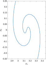
(a) $N=64$

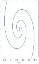
(b) $N=128$

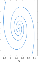
(c) $N=256$

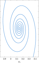
(d) $N=512$

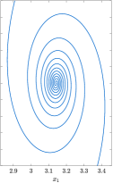
(e) $N=1024$

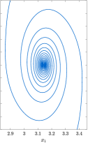
(f) $N=2048$

Figure 3: Numerical simulation of a KHI test using the $z$-model with the Krasny desingularization. Shown is the interface position $z(\alpha,t)$ at time $t=3.0$ for six simulations with resolution starting from $N=64$ and doubling until $N=2048$.

Next, we consider the convergence of the numerical solution as $\delta\,,N^{-1}\to 0$. The convergence of solutions as $\delta\to 0$ with $N$ fixed is considered in detail in [56, 8], wherein it is shown that the computed numerical solution appears to converge.

In Figure 4(a), we show how the amplitude $\max z_{2}$ of the curve varies as $\delta,N^{-1}\to 0$. The value for $N^{-1}$ is obtained by cubic extrapolation. We see that the amplitude appears to converge to a finite value $\approx 0.81$. Similarly, in Figure 4(b), we estimate the radius of the spiral region by $r_{\delta}\approx\pi-\min x_{1}^{*}$, where $x^{*}$ are the intersection points with the axis $x_{2}=x_{2}^{*}=0$. By symmetry, the center of the spiral is located at $(\pi,0)$. Again, with the value for $N^{-1}=0$ obtained by cubic extrapolation, we see that the $r_{\delta}$ appears to converge to a value close to 0.28. This demonstrates that the scaling (31) appears to be appropriate for recovering a meaningful solution as $\delta,N^{-1}\to 0$.

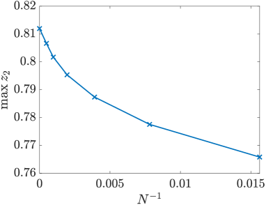
(a) Amplitude $\max z_{2}$.

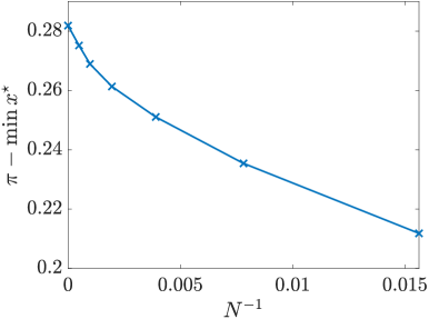
(b) Radius of the spiral region $r_{\delta}\approx\pi-\min x_{1}^{*}$.

Figure 4: Convergence behavior for a KHI test using the $z$-model with the Krasny desingularization. Shown are (a) the amplitude of the curve $\max z_{2}$ and (b) the radius of the spiral region $r_{\delta}$.

4.3.3.  Single-mode RTI: comparison with experiments

We continue our numerical studies for the $z$-model by performing simulations for the low Atwood number single-mode RTI experiments of Waddell et al. [104]. The particular problem setup considered is a heavy fluid lying atop a lighter fluid, with the Atwood number given by $A=0.155$ and the two fluids subject to an approximately constant gravitational acceleration $g=0.74\times 9.8\mathrm{ms}^{-2}$. The $z$-model is employed for this problem on the domain $\alpha\in[-0.027,0.027]$ with initial data

$$z_{1}(\alpha,0) =\alpha\,,$$

$$z_{2}(\alpha,0) =0.0012\cos(2\pi\alpha/L)\,,$$

$$\varpi(\alpha,0) =0\,.$$

We perform six simulations with resolution starting from $N=32$ and doubling until $N=1024$. The strategy for parameter choice we adopt here is to keep the parameters $\tilde{\delta}=2$ and $\tilde{\mu}=0.02$ fixed as $N$ varies, while allowing the time-steps $\delta t$ to vary with $N$. Specifically, we first choose $\delta t$ for $N=64$ as the largest possible value that will allow the $N=64$ simulation to run until the final time $t=0.3795$. The values of $\delta t$ for larger $N$ are then determined by repeatedly halving this value until $\delta t$ is sufficiently small so as to allow the simulation to complete.

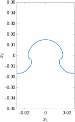
(a) $N=32$

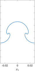
(b) $N=64$

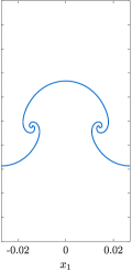
(c) $N=128$

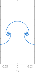
(d) $N=256$

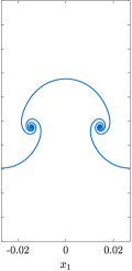
(e) $N=512$

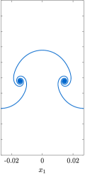
(f) $N=1024$

Figure 5: Numerical simulation of the Waddell et al. [104] RTI using the $z$-model. The interface parameterizations $z(\alpha,t)$ for six simulations with resolution starting from $N=32$ and doubling until $N=1024$ are shown at time $t=0.3795$.

Figure 6: Closeup view of the roll-up region for $N=1024$.

The results of the six simulations are shown in Figure 5, which should be compared with Figure 4(l) of [104]. The bubble and spike shapes are roughly symmetric, in agreement with the observations in [104]. The scaling for the regularization parameters $\tilde{\delta}$ and $\tilde{\mu}$ results in more roll-up of the vortex sheet as the resolution is increased. This is demonstrated in Figure 6, which shows that the interface for the $N=1024$ simulation has a tightly packed spiral region with several complete revolutions of each branch of the spiral.

We next compare the growth rate of the $z$-model solution interface with growth rates obtained from small-time linear theory predictions and late-time experimental observations. Define the amplitude of the interface as $a(t)=\frac{1}{2}\left[\max_{\alpha}z_{2}(\alpha,t)-\min_{\alpha}z_{2}(\alpha,t)\right]$. Linear theory [67, 96] predicts that for early times $t$ before the non-linearity is activated, the amplitude satisfies $a(t)=a(0)\cosh(t\sqrt{2\pi Ag/L})$. We plot in Figure 7(a) the linear theory amplitude and the computed amplitude $a(t)$ versus time for the simulations shown in Figure 5. It is clear from the graph that the computed amplitude and linear prediction are in excellent agreement, as expected, for small times $t\leq 0.15$.

For large times, the nonlinearity is no longer negligible and the linear theory breaks down. Experimental observations indicate that the amplitude grows linearly at late times; a linear fit of the measured late time amplitude from experimental data is shown as the blue curve in Figure 7(b). This curve is defined in [104] as $-0.007436+0.078177t$. It is clear from the graph that the measured amplitude differs considerably from the amplitude computed using the $z$-model. This difference may be explained by the fact that the (effective) gravitational acceleration in the experiments is only approximately constant, and is in fact time-dependent, whereas we have used a constant value of $g$.

While the amplitudes themselves differ, we nonetheless observe that the growth rates of the computed amplitude and measured amplitude are in excellent agreement. The green curve shown in Figure 7(b) has the same slope as the blue curve (i.e. the measured amplitude) and is given explicitly as $-0.01115+0.078177t$. This curve matches almost exactly with the computed $a(t)$ for large times $t\geq 0.25$. In fact, the true gravitational acceleration in the experimental setup is initially time-dependent, but eventually reaches a constant value; in our numerical simulation, we have used this final constant value for $g$, which is why the amplitude of the numerical solution at large times $t\geq 0.25$ grows at the same rate as that observed in the experiment. The numerical solution and the experimental data are thus in good agreement (modulo the issue regarding the non-constant value of $g$), which consequently provides validating evidence for the $z$-model.

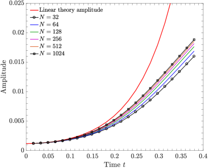
(a) Comparison of the computed amplitude and linear theory predictions for the simulations in Figure 5.

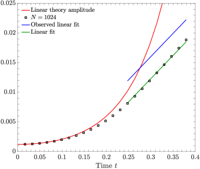
(b) Comparison of the computed amplitude for the $N=1024$ simulation with large time linear fits.

Figure 7: Plots of the amplitude $a(t)$ versus time $t$ for the Waddell et al. [104] RTI problem.

Next, we consider the convergence of the computed numerical solution in the limits $\delta\to 0$ with $N=256$ fixed. Figure 8(a) shows that the bubble and spike tip locations appear to converge linearly, which agrees with the results of [56] for the KHI test. Here, the value at $\delta=0$ is obtained by linear extrapolation. In Figure 8(b) and Figure 8(c), we show the convergence of the computed spiral center $\sigma_{\delta}$ and radius $r_{\delta}$. We choose the axis $x_{2}=x_{2}^{*}=-0.0023$ to compute the intersection points $x^{*}$. Again, the computed values appear to converge, though the precise nature of this convergence is less clear. In this case, we obtain the value at $\delta=0$ via cubic interpolation.

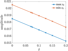
(a) Bubble and spike tip locations.

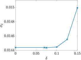
(b) Location of spiral center $\sigma_{\delta}$.

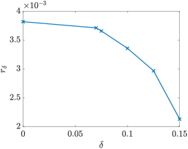
(c) Radius of spiral $r_{\delta}$.

Figure 8: Convergence behavior for the RTI test of Waddell et al. [104] using the $z$-model with the Krasny desingularization. Shown are (a) the bubble and spike tip locations, $|\max z_{2}|$ and $|\min z_{2}|$, respectively, (b) the location of the center of the spiral region $\sigma_{\delta}$, and (c) the radius of the spiral region $r_{\delta}$.

We repeat our convergence tests for $N=256$ fixed and $\delta\to 0$ with the kernels (34), and compare the results with the Krasny kernel results in Figure 9. We find excellent agreement between all three methods in the limiting behavior of the bubble and spike tip locations, as shown in Figure 9(a); this is in agreement with previous numerical studies [8, 93]. The small scale structure of the limiting solutions are slightly different, with the Krasny kernel and first order kernel $\mathcal{K}_{1}^{\delta}$ producing similar spiral center locations $\sigma_{\delta}$ and radii $r_{\delta}$. Here, the value at $\delta=0$ is obtained by cubic extrapolation. Let us note that for $\delta>0$, all three methods predict similar values of $\sigma_{\delta}$ and $r_{\delta}$.

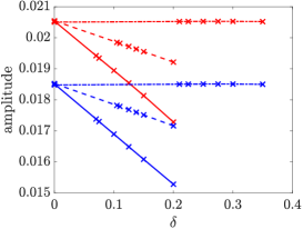
(a) Bubble (blue) and spike (red) tip locations.

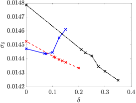
(b) Location of spiral center $\sigma_{\delta}$.

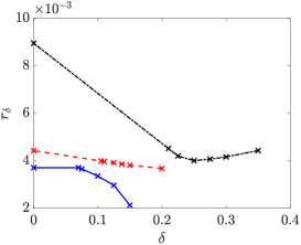
(c) Radius of spiral $r_{\delta}$.

Figure 9: Convergence behavior as $\delta\to 0$ with $N=256$ fixed for the RTI test of Waddell et al. [104] using the $z$-model. Shown are (a) the bubble and spike tip locations, $|\max z_{2}|$ and $|\min z_{2}|$, respectively, (b) the location of the center of the spiral region $\sigma_{\delta}$, and (c) the radius of the spiral region $r_{\delta}$. The solid, dashed, and dotted curves in (a) refer to the Krasny, $\mathcal{K}^{\delta}_{1}$, and $\mathcal{K}^{\delta}_{3}$ kernels, respectively. The blue, red, and black curves in (b) and (c) refer to the Krasny, $\mathcal{K}^{\delta}_{1}$, and $\mathcal{K}^{\delta}_{3}$ kernels, respectively.

Next, we consider the limit $\delta,N^{-1}\to 0$, simultaneously; for the Krasny kernel, we use the scaling (31), while for the kernels $\mathcal{K}^{\delta}_{i}$ we use the empirical procedure discussed at the beginning of Section 4.3. We consider six simulations with resolution starting from $N=32$ and doubling until $N=1024$, and again compute the bubble/spike tip locations and quantities $\sigma_{\delta}$ and $r_{\delta}$. We find excellent agreement between all three methods for the limiting values of each of the relevant quantities. Moreover, the Krasny scheme is the least computationally expensive method: for the $N=1024$ simulation, the runtime for the Krasny scheme is $T_{\mathrm{CPU}}\approx 333$ s, whereas the runtime for the 3rd order kernel $\mathcal{K}^{\delta}_{3}$ scheme is $T_{\mathrm{CPU}}\approx 469$ s, and thus the simpler Krasny scheme is 40% faster. As such, we conclude that, as the simplest and least computationally expensive method, the Krasny desingularization is the most suitable method for our objective.

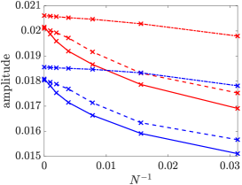
(a) Bubble (blue) and spike (red) tip locations.

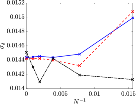
(b) Location of spiral center $\sigma_{\delta}$.

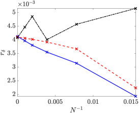
(c) Radius of spiral $r_{\delta}$.

Figure 10: Convergence behavior as $\delta,N^{-1}\to 0$ for the RTI test of Waddell et al. [104] using the $z$-model. Shown are (a) the bubble and spike tip locations, $|\max z_{2}|$ and $|\min z_{2}|$, respectively, (b) the location of the center of the spiral region $\sigma_{\delta}$, and (c) the radius of the spiral region $r_{\delta}$. The solid, dashed, and dotted curves in (a) refer to the Krasny, $\mathcal{K}^{\delta}_{1}$, and $\mathcal{K}^{\delta}_{3}$ kernels, respectively. The blue, red, and black curves in (b) and (c) refer to the Krasny, $\mathcal{K}^{\delta}_{1}$, and $\mathcal{K}^{\delta}_{3}$ kernels, respectively.

4.3.4.  Single-mode RTI: comparison with numerical simulations

Next, we compare the numerical simulations of Sohn [92] that used the discretized equations (22), with our higher-order z-model solutions. A brief description of the numerical method in [92] is as follows. The $z$-equation (22a) is treated in an identical fashion as in our numerical framework; in particular, the same Krasny $\delta$-desingularization and trapezoidal rule is used. The $\varpi$-equation (22b) is discretized in physical space, rather than in Fourier space as in our numerical method. The nonlinear term is treated using upwinding via the Godunov method, while an iterative procedure is used for the time-derivative term appearing on the right-hand side of (22b). Let us remark that, on average, 6 iterations per time-step are required for this numerical method.

Since we are interested in capturing vortex sheet roll-up, we consider the low Atwood number RTI test problem from [92]. The domain is $\alpha\in[-\pi,\pi]$, the Atwood number is $A=0.05$, the gravitational constant is $g=1$, and the initial data is

$$z_{1}(\alpha,0) =\alpha\,,$$

$$z_{2}(\alpha,0) =0.5\cos(\alpha)\,,$$

$$\varpi(\alpha,0) =0\,.$$

The $z$-model is run for this problem with $N=400$, which is the same value employed in [92], but whereas the value $\delta t=0.002$ is required in [92], we are able to use the much larger $\delta t=0.025$. The regularizing parameters chosen as $\tilde{\delta}=0.6$ and $\tilde{\mu}=0.005$. This value of $\tilde{\delta}$ was chosen to agree with the parameter choices in [92].

The computed $z$ for the above numerical experiment is shown in Figure 11 at various time $t$. This figure should be compared with Figure 1(a) in [92], upon which it is clear that the two are essentially indistinguishable. In particular, we note that the two solutions are in excellent agreement in the roll-up region, with both branches of the spirals having almost four full rotations at the final time $t=22$.

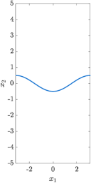
(a) $t=0$

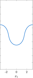
(b) $t=10$

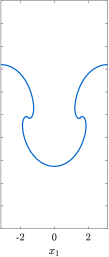
(c) $t=14$

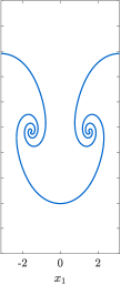
(d) $t=18$

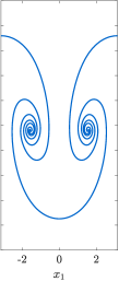
(e) $t=22$

Figure 11: Numerical simulation of the RTI using the $z$-model with the setup as in the numerical studies of Sohn [92]. Plots of the interface $z$ for a simulation with Atwood number $A=0.05$ are shown at various times $t$.

To quantify the agreement between our $z$-model solution and the reference solution from [92], we plot various computed quantities in Figure 12. The bubble tip and spike tip speeds versus time are shown in Figure 12(a) (compare with Figure 3(a) in [92]). Shown also are theoretical predictions for the bubble speed from asymptotic potential flow models. Such models aim to describe analytically the evolution of the amplitude of the interface $z$, after the transition from exponential growth $z\sim z_{0}e^{t\sqrt{Ag}}$ at small times (as predicted by the linear theory) to linear-in-time growth $z\sim w_{\infty}t$ (as observed in experiments, for instance), where $w_{\infty}$ is the asymptotic bubble velocity. The Goncharov [42] and Sohn [91] models estimate $w_{\infty}$ as

$$w_{\infty}=\sqrt{\frac{2A}{1+A}\frac{g}{3}}\qquad\text{ and }\qquad w_{\infty}=\sqrt{\frac{Ag}{2+A}}\,,$$

respectively. As shown in Figure 12(a), the computed speed and asymptotic predictions are in good agreement; let us note that the bubble and spike speeds computed using the $z$-model appear identical to those in [92].

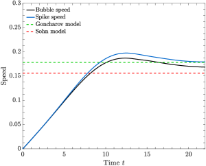
(a) Bubble and spike speeds

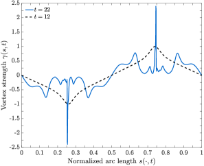
(b) Vortex strength

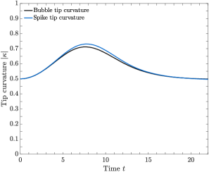
(c) Tip curvature

Figure 12: Plots of various computed quantities for the Sohn [92] RTI problem.

Next, we compute the vortex sheet strength $\gamma(\cdot,t)=\varpi(\cdot,t)/|\partial_{\alpha}z(\cdot,t)|$. We plot $\gamma(s,t)$ versus $s$ in Figure 12(b), where $s(t)$ is the normalized arclength. Comparing Figure 12(b) with Figure 7(a) in [92], we see that $\gamma(s,t)$ computed using the $z$-model is slightly larger in magnitude at the shock, but is otherwise identical to the solution in [92]. Finally, we compute the magnitude of the bubble tip and spike tip curvatures $|\kappa|$ in Figure 12(c), which is in excellent agreement with Figure 6(a) in [92].

The above observations indicate that the $z$-model is able to accurately simulate interface turnover and roll-up, while minimizing the cost of the numerical computations. In particular, since six iterations are required, on average, for the algorithm in [92], the $z$-model computation is at least 6 times faster if the same time-step $\delta t$ used. For the above simulation, we were able to use a much larger time-step, which shows that that the $z$-model computation is a factor of at least $6\times 0.025/0.002=75$ times faster. In fact, since the Fast Fourier Transform (FFT) is used to efficiently compute the $\varpi$-equation (38), whereas costly upwinding is required for the algorithm in [92], it is highly likely that the $z$-model computation is much greater than 75 times faster than the algorithm in [92].

4.3.5.  Multi-mode RTI: the rocket rig experiment of Read and Youngs

We next consider the rocket rig experiment of Read [79] and Youngs [106], in which the initial interface separating the two fluids of densities $\rho^{+}$ and $\rho^{-}$ is given by a small and random perturbation of the flat interface. Our aim is to compare the growth rates of the mixing layer computed using our $z$-model with the growth rates observed in experiments [79] and 2-$D$ DNS simulations [106]. The experimental and numerical evidence indicate that the width of the mixing layer grows like

$$\Theta Agt^{2}\,,$$ (43)

where $\Theta$ is some constant. The experimental evidence suggests that the constant $\Theta$ lies in the range $\Theta\in(0.05,0.775)$, while the numerical simulations give $\Theta\in(0.04,0.05)$. We shall follow Youngs [107], and employ the value $\Theta=0.06$ for comparison purposes.

We set up the problem as follows: the domain is $\alpha\in[-\pi,+\pi]$, the densities of the two fluids are $\rho^{+}=0.66$ and $\rho^{-}=1.89$, giving an Atwood number of $A\approx 0.482$, the gravitational acceleration is $g=-9.8\times\frac{2\pi}{0.3}$, and the initial data is given by

$$z_{1}(\alpha,0) =\alpha\,,$$

$$z_{2}(\alpha,0) =\frac{1}{\sigma}\sum_{r=1}^{s}a_{r}\cos(r\alpha)+b_{r}\sin(r\alpha)\,,$$

$$\varpi(\alpha,0) =0\,,$$

where $a_{r}$ and $b_{r}$ are random number chosen from a standard Gaussian distribution, $s=32$, and $\sigma$ is a constant chosen such that $||z_{2}(\cdot,0)||_{L^{2}}=0.01$.

	$N$
	128	256	512	1024	2048
$\delta t$	$1\times 10^{-3}$	$1\times 10^{-3}$	$5\times 10^{-4}$	$1.25\times 10^{-4}$	$3.125\times 10^{-5}$

Table 2: Time-step $\delta t$ choices for the rocket rig test.

We perform 5 simulations using the $z$-model and with resolution starting from $N=128$ and doubling until $N=2048$. The regularization parameters are fixed as $\tilde{\delta}=0.065$ and $\mu=0.06$ for all of the simulations. The time-step $\delta t$ varies with $N$, and is listed in Table 2. We show plots of the computed interface parametrization $z(\alpha,t)$ at the final time $t=0.15$ in Figure 13. As expected, there is more-roll up of the interface as the resolution is increased. To quantify the amount of mixing, the width of the mixing region is approximated as $\max_{\alpha}z_{2}(\alpha,t)-\max_{\alpha}z_{2}(\alpha,0)$. A comparison of the computed mixing region width and the predicted quadratic growth rate (43) with $\Theta=0.06$ is shown in Figure 14, from which it is clear that the two are in very good agreement.

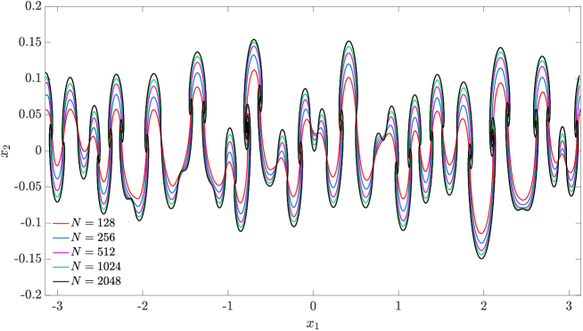
Figure 13: Numerical simulation of the rocket rig test using the $z$-model. The results for five simulations with resolution starting from $N=128$ and doubling until $N=2048$ are shown at time $t=0.15$.

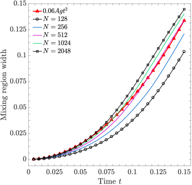
Figure 14: Plot of the mixing region width $\max z_{2}(\cdot,t)-\min z_{2}(\cdot,0)$ versus time $t$ for the rocket rig test. Results are shown for five simulations using the $z$-model with increasing resolution $N$. The red curve is the predicted quadratic growth rate (43) with $\Theta=0.06$.

Since the initial conditions for the rocket rig test are random, it may be difficult to obtain a clear qualitative picture of the mixing region from a single simulation alone. Consequently, we repeat the test for $N=512$ with six different random initial conditions. The interface position for the ensemble of runs is shown in Figure 15(a), while the mean mixing region width is compared with the quadratic growth rate in Figure 15(b). It is clear from Figure 15(b) that the computed mixing region width is in excellent agreement with the predicted quadratic growth rate, thus providing strong evidence for the validity of the $z$-model. The average runtime for the $N=512$ simulations is only $T_{\mathrm{CPU}}\approx 20\mathrm{s}$; thus, the use of the $z$-model permits the inference of large-scale qualitative and quantitive information with minimal computational expense.

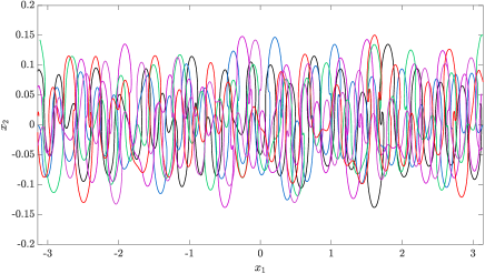
(a) Interface position $z$

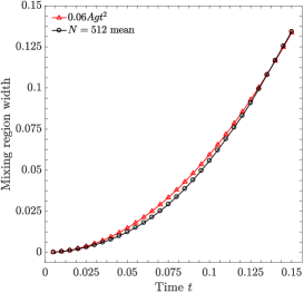
(b) Mean mixing region width

Figure 15: Ensemble of simulations for the rocket rig test with $N=512$. Shown are (a) the interface position $z$ at time $t=0.15$, and (b) the mean mixing region width versus time.

5.  A mutliscale model for interface evolution in compressible flow

We now derive a multiscale interface model, founded upon our incompressible-compressible decomposition of the Euler equations. The discontinuous incompressible velocity $w$ solving (27) (and, in particular, obtained from (24)) can be used to compute small scale structures on the interface $\Gamma(t)$ and the Kelvin-Helmholtz instability (KHI). It is often the case that vortex sheet roll-up, caused by the KHI, occurs at spatial scales which are smaller than the scales along which bulk vorticity is transported and for which sound waves propagate. When this occurs, the continuous velocity $v$ solving (28), which is only forced by bulk compression and vorticity, may be computed at larger spatial scales than the velocity $w$.

5.1.  A multiscale model for the compressible RTI

In order to produce a fast-running model of the compressible RTI, we begin by using the higher-order $z$-model (24) to generate the velocity $w$. Our model is generated by coupling the equation for $v$ (28) together with

$$\partial_{t}z(\alpha,t) =\operatorname{P}\int_{\mathbb{T}_{L}}\mathcal{K}_{\mathbb{T}_{L}}(z(\alpha,t)-z(\beta,t))\varpi(\beta,t)\,\mathrm{d}\beta+v(z(\alpha,t),t)\,,$$ (45a)

$$\partial_{t}\varpi(\alpha,t) =-\partial_{\alpha}\left[\frac{A}{2|\partial_{\alpha}z(\alpha,t)|^{2}}\mathcal{H}\left(\varpi(\alpha,t)\mathcal{H}\varpi(\alpha,t)\right)-2Agz_{2}(\alpha,t)\right]\,,$$ (45b)

and computing $w$ using (19). As we explain below, the compressible equations (28) will be solved on a coarse grid, while (45) will be solved on a fine, but one-dimensional, grid.

5.2.  A multiscale model for the compressible RMI

5.2.1.  Vorticity production

For flows in which shock waves collide with contact discontinuities and initiate the RMI, we shall derive a modified form of the $z$-model which accounts for the vorticity production that is caused by the misalignment of the pressure gradient at the shock wave and the density gradient at the interface.

Computing the curl of (15b), we obtain the two-dimensional vorticity equation for compressible flow as

$$\frac{\mathrm{D}\omega}{\mathrm{D}t}+\omega\operatorname{div}u=-\frac{\nabla\rho\cdot\nabla^{\perp}p}{\rho^{2}}\,.$$ (46)

The term on the right-hand side of (46) is the baroclinic term, responsible for vorticity production on the interface when a shock-wave collides with a vortex sheet. The amplitude of vorticity $\varpi$ is the weak (or distributional) form of the vorticity, and consequently it is important to include a weak form of the baroclinic term in the dynamics of $\varpi$. We thus introduce the following modification of the $z$-model

$$\partial_{t}z(\alpha,t) =\operatorname{P}\int_{\mathbb{T}_{L}}\mathcal{K}_{\mathbb{T}_{L}}(z(\alpha,t)-z(\beta,t))\varpi(\beta,t)\,\mathrm{d}\beta+v(z(\alpha,t),t)\,,$$ (47a)

$$\partial_{t}\varpi(\alpha,t) =-\partial_{\alpha}\left[\frac{A}{2|\partial_{\alpha}z(\alpha,t)|^{2}}\mathcal{H}\left(\varpi(\alpha,t)\mathcal{H}\varpi(\alpha,t)\right)-2Agz_{2}(\alpha,t)\right]$$

$$\qquad\qquad-\llbracket\nabla p\cdot\partial_{\alpha}z(\alpha,t)/\rho\rrbracket+\mu\partial^{2}_{\alpha}\varpi(\alpha,t)\,,$$ (47b)

which will be used for flows in which shocks collide with contact discontinuities.

Remark 1.

Let us mention that for Richtmyer-Meshkov problems, at the time at which the planar shock collides with the perturbed contact, the pressure is discontinuous along points in the intersection of the shock and contact. As such the numerator in the baroclinic term, $\llbracket\nabla p\cdot\partial_{\alpha}z(\alpha,t)\rrbracket$ can be large at such points. Such a pressure profile does not occur in the Rayleigh-Taylor problems, for which the numerator $\llbracket\nabla p\cdot\partial_{\alpha}z(\alpha,t)\rrbracket$ vanishes along the contact. Thus, the use of this baroclinic term in the $\varpi$-equation is imperative for the simulation of the RMI problems.

5.2.2.  Taylor’s frozen turbulence hypothesis

Taylor’s “frozen turbulence” hypothesis [95], roughly speaking, states that if the mean flow velocity is much larger than the velocity of the turbulent eddies, then the advection of the turbulent flow past a fixed point can be taken to be due entirely to the mean flow, or in other words, that the turbulent fluctuations are transported by the mean flow. For shock-contact collisions that initiate the RMI, the velocity $v$ at the shock front is much larger in magnitude than the velocity $w$. That is to say, the relation $\max_{x}|v|\gg\max_{x}|w|$ holds true. For instance, for the RMI problem considered in Section 6.4, the quantity $\max_{x}|w|$ is two orders of magnitude smaller than the quantity $\max_{x}|v|$. For such flows, we view the velocity $v$ as the mean velocity and $w$ as the fluctuation velocity, and impose the Taylor hypothesis that for very short time-intervals (i.e., about one time-step in an explicit numerical simulation), $w$ is transported by $v$, so that

$$\partial_{t}w+(v\cdot\nabla)w=0\,.$$ (48)

As we described in Remark 1, at points along the interface at which the shock front intersects the contact discontinuity, there exists a large increase in the baroclinic term, which in turn, produces a large increase in the amplitude of vorticity and this then leads to a localized increase in the small-scale velocity field $w$ via equation (47b) at each such intersection point at each time-step. As the shock passes through the contact discontinuity these points of intersection evolve, and this evolution causes large (and localized) space gradients $\nabla w$ and temporal gradients $\partial_{t}w$. The Taylor hypothesis (48) ensures that a proper balance is retained between the space and time gradient of $w$ in a numerical implementation which approximates these two different types of derivatives in a very different manner.

Using (48) together with (28a), we find that

$$\partial_{t}(\rho w)+\operatorname{div}(\rho w\otimes v)+\operatorname{div}(\rho w\otimes w)=\rho(w\cdot\nabla)w\,,$$

and hence (28b) must be replaced by

$$\partial_{t}(\rho v)+\nabla\cdot(\rho v\otimes v)+\nabla p+\rho ge_{2}=-\nabla\cdot(\rho v\otimes w)-\rho(w\cdot\nabla)w\,.$$ (28b’)

Therefore, our model for the RMI problem couples (47) with (28), but with (28b’) replacing (28b). Using a Richtmyer-Meshkov test problem, we explain in detail in Section 6.4 the reasons for using the Taylor hypothesis and (28b’) in our multiscale algorithm for RMI flows.

5.3.  The multiscale algorithms for the RTI and RMI problems

We are now ready to give a precise description of the multiscale algorithm. Denote by ${\bf V}(x,t)=(\rho,\rho v_{1},\rho v_{2},E)^{\mathcal{T}}$, the solutions to the compressible equations (28). We shall use a standard 3rd order Runge-Kutta procedure for time-integration; in the following algorithms, we use the superscript notation to denote the Runge-Kutta stage.

We shall use two slightly different algorithms; the first is for our multiscale model for RTI problems, while the second is for the multiscale model for RMI problems.

We note that the ordering of Steps Step 44(b), Step 44(c), and Step 44(d) in the RTI multiscale algorithm is important; our numerical experiments have shown that it is important that the velocity $w^{\prime}(x)$ is computed before the auxiliary interface $\tilde{z}$ is updated.

For Richtmyer-Meshkov problems, we use a slightly different algorithm. In particular, we are no longer required to compute the time-derivative $\partial_{t}(\rho w)$ and so shall omit those steps from the algorithm. Notice that this means that we can omit in particular Step Step 44(b) of the RTI algorithm, which removes at each time-step one of the costly integral computations. On the other hand, we must compute in Step Step 44(d) of the RMI algorithm the baroclinic term in the $\varpi$-equation (47).

Remark 2.

In this work, we apply our multiscale algorithm to 2-$D$ flows that are symmetric across the line $x_{1}=0$. In particular, this means that the velocities $w_{1}$ and $v_{1}$ are odd functions of $x_{1}$, and the vorticity amplitude $\varpi$ is an odd function of $\alpha$.

RTI Multiscale Algorithm

1. Suppose that we are given the solution $z(\alpha,t)$, $\varpi(\alpha,t)$, and $\mathbf{V}(x,t)$ at time-step $t$, as well as a velocity ${w^{\prime}}(x)$, and we wish to compute the solution at $t+\delta t$. Define $z^{0}(\alpha)\coloneqq z(\alpha,t)$, $\varpi^{0}(\alpha)\coloneqq\varpi(\alpha,t)$, and $\mathbf{V}^{0}(x)\coloneqq\mathbf{V}(x,t)$, and let $\rho^{\prime}(x)\coloneqq\rho^{0}(x)=\rho(x,t)$.

2. 1. Compute a velocity $\tilde{w}(x)$ from $z^{0}(\alpha)$ and $\varpi^{0}(\alpha)$ using the Biot-Savart law.

   2. Approximate $\partial_{t}(\rho\tilde{w})(x)=\left[\rho^{0}(x)\tilde{w}(x)-\rho^{\prime}(x)w^{\prime}(x)\right]/\delta t$.

   3. Solve the compressible equations (28) (with $w=\tilde{w}$) to obtain $\mathbf{V}^{1}(x)$.

   4. Compute an auxiliary $\tilde{z}(\alpha)$ and $\varpi(\alpha)$ by solving the system (45).

   5. Calculate the interfacial velocity $v(\tilde{z}(\alpha))=v^{1}(x)|_{\tilde{z}(\alpha)}$ using interpolation.

   6. Update $z^{1}(\alpha)=\tilde{z}(\alpha)+\delta t\cdot v(\tilde{z}(\alpha))$, and set $\varpi^{1}(\alpha)=\tilde{\varpi}(\alpha)$.

3. Repeat Step 1 but with quantities evaluated at the next Runge-Kutta stage.

4. Repeat Step 2 but with quantities evaluated at the next Runge-Kutta stage.

5. 1. Use the standard 3rd order Runge-Kutta formula to produce $\mathbf{V}(x,t+\delta t)$, and an auxiliary interface $\tilde{z}(\alpha)$ and vorticity amplitude $\varpi(\alpha)$.

   2. Compute a velocity $w^{\prime}(x)$ from $\tilde{z}(\alpha)$ and $\tilde{\varpi}(\alpha)$ using the Biot-Savart law.

   3. Calculate the interfacial velocity $v(\tilde{z}(\alpha))=v(x,t+\delta t)|_{\tilde{z}(\alpha)}$ using interpolation.

   4. Update $z(\alpha,t+\delta t)=\tilde{z}(\alpha)+\delta t\cdot v(\tilde{z}(\alpha))$, and set $\varpi(\alpha,t+\delta t)=\tilde{\varpi}(\alpha)$, then return to Step 0.

RMI Multiscale Algorithm

1. Suppose that we are given the solution $z(\alpha,t)$, $\varpi(\alpha,t)$, and $\mathbf{V}(x,t)$ at time-step $t$, as well as the baroclinic term $\phi(\alpha,t)=\llbracket\nabla p\cdot\partial_{\alpha}z/\rho\rrbracket$ and we wish to compute the solution at $t+\delta t$. Define $z^{0}(\alpha)\coloneqq z(\alpha,t)$, $\varpi^{0}(\alpha)\coloneqq\varpi(\alpha,t)$, and $\mathbf{V}^{0}(x)\coloneqq\mathbf{V}(x,t)$.

2. 1. Compute a velocity $\tilde{w}(x)$ from $z^{0}(\alpha)$ and $\varpi^{0}(\alpha)$ using the Biot-Savart law.

   2. Solve the modified compressible equations (28) (with $w=\tilde{w}$), using (28b’) in place of (28b), to obtain $\mathbf{V}^{1}(x)$.

   3. Compute an auxiliary $\tilde{z}(\alpha)$ and $\varpi(\alpha)$ by solving the system (47).

   4. Calculate an auxiliary baroclinic term $\tilde{\phi}(\alpha)$ using $\tilde{z}(\alpha)$, $p^{1}(x)$, and $\rho^{1}(x)$.

   5. Calculate the interfacial velocity $v(\tilde{z}(\alpha))=v^{1}(x)|_{\tilde{z}(\alpha)}$ using interpolation.

   6. Update $z^{1}(\alpha)=\tilde{z}(\alpha)+\delta t\cdot v(\tilde{z}(\alpha))$, and set $\varpi^{1}(\alpha)=\tilde{\varpi}(\alpha)$.

3. Repeat Step 1 but with quantities evaluated at the next Runge-Kutta stage.

4. Repeat Step 2 but with quantities evaluated at the next Runge-Kutta stage.

5. 1. Use the standard 3rd order Runge-Kutta formula to produce $\mathbf{V}(x,t+\delta t)$, and an auxiliary interface $\tilde{z}(\alpha)$ and vorticity amplitude $\varpi(\alpha)$.

   2. Calculate the interfacial velocity $v(\tilde{z}(\alpha))=v(x,t+\delta t)|_{\tilde{z}(\alpha)}$ using interpolation.

   3. Update $z(\alpha,t+\delta t)=\tilde{z}(\alpha)+\delta t\cdot v(\tilde{z}(\alpha))$, and set $\varpi(\alpha,t+\delta t)=\tilde{\varpi}(\alpha)$.

   4. Compute the baroclinic term $\phi(\alpha,t+\delta t)$ using $z(\alpha,t+\delta t)$, $p(x,t+\delta t)$, and $\rho(x,t+\delta t)$, then return to Step 0.

5.4.  Numerical implementation of the multiscale algorithm

We now describe how we numerically implement the multiscale algorithm described in Section 5. Suppose that the conservative variables ${\bf V}$ are computed in the bounded domain $\Omega=\mathbb{T}_{L}\times[x^{1}_{2}\,,x^{n}_{2}]$, and that the flow is periodic in the horizontal variable $x_{1}$. Suppose also that a single wavelength of the periodic interface $\Gamma(t)$ is parametrized by the function $z(\alpha,t)$.

Discretize the domain $\Omega$ with $(2m-1)\times n$ cells with cell centers at

$$x^{i}_{1} =-L/2+(i-1)\delta x_{1}\,,$$

$$x^{j}_{2} =x^{1}_{2}+(j-1)\delta x_{2}\,,$$

with $\delta x_{1}=L/(2m-2)$ and $\delta x_{2}=(x^{n}_{2}-x^{1}_{2})/(n-1)$, and suppose that the parameter $\alpha$ is discretized with $N=2^{r}+1$ nodes,

$$\alpha_{k}=-L/2+(k-1){\scriptstyle\Delta}\alpha\,,$$

with ${\scriptstyle\Delta}\alpha=L/(N-1)$. We spatially discretize the equations of motion, then use a standard third-order explicit Runge-Kutta solver for time integration. We shall use a space-time smooth artificial viscosity method, which we call the $C$-method [78], for the compressible $v$-equations (28) to stabilize shock fronts and contact discontinuities, and thereby prevent the onset of Gibbs oscillations.

It remains to describe the following: first, the numerical implementation of the space-time smooth artificial viscosity $C$-method; second, the computation of the velocity $w$ on the plane; third, the bilinear interpolation scheme; and finally, the calculation of the weak baroclinic term $\llbracket\nabla p\cdot\partial_{\alpha}z/\rho\rrbracket$.

5.4.1.  Numerical implementation of the $C$-method

We implement a simple finite difference WENO-based scheme to spatially discretize the system (28). Our simplified WENO scheme is devoid of any exact or approximate Riemann solvers, and instead relies on the sign of the velocity to perform upwinding. A fourth-order central difference approximation is used to compute the pressure gradient $\nabla p$, while a second-order central difference approximation is employed to compute the diffusion terms (60). For brevity, we omit further details of the numerical implementation of the $C$-method and refer the reader to Appendix B and [78] for further details.

5.4.2.  Computing the $w$ velocity

We first describe our method for calculating the discrete velocity $w_{i,j}=w(x_{1}^{i},x_{2}^{j})$ from a given discretized interface parametrization $z_{k}$ and vorticity amplitude $\varpi_{k}$.

Since integral-kernel calculations can be computationally very expensive, we begin by proposing a simplification to speed up such calculations. Suppose first that we wish to compute the velocity $w$ at a point $x_{i,j}$ such that $|x_{2}^{j}-z_{2}^{k}|\gg 1$ for every $k$. Then the following approximations are valid:

$$-\frac{\sinh(2\pi(x^{j}_{2}-z_{2}^{k})/L)}{\cosh(2\pi(x^{j}_{2}-z_{2}^{k})/L)-\cos(2\pi(x^{i}_{1}-z_{1}^{k})/L)}\approx\pm 1\,,$$

$$\frac{\sin(2\pi(x^{i}_{1}-z_{1}^{k})/L)}{\cosh(2\pi(x^{j}_{2}-z_{2}^{k})/L)-\cos(2\pi(x^{i}_{1}-z_{1}^{k})/L)}\approx 0\,.$$

Then, using the fact that $\varpi$ is an odd function (c.f. Remark 2), it follows that $w_{i,j}\approx 0$. Consequently, it is sufficient to compute $w$ only for those $x_{i,j}$ that lie in the horizontal strip

$$\Omega_{z}=\left\{x\in\mathbb{T}_{L}\times[x_{2}^{1},x_{2}^{n}]\text{ s.t. }\min_{k}z^{k}_{2}-\lambda\leq x_{2}\leq\max_{k}z^{k}_{2}+\lambda\right\}\,.$$

For the simulations considered here, we set $\lambda=0.075$, but note that this parameter is problem dependent. Computing the velocity only in the strip $\Omega_{z}$ speeds up an otherwise time-consuming calculation.

We now define the scalar function $\mathcal{J}^{\delta}(x)$ by

$$\mathcal{J}^{\delta}(x)=\frac{1}{4\pi}\log\left\{\delta^{2}+\cosh(2\pi x_{2}/L)-\cos(2\pi x_{1}/L)\right\}\,.$$

The function $\mathcal{J}^{\delta}$ is a smoothed version of the singular kernel used in the integral representation of $\Delta^{-1}$, so that $\mathcal{K}^{\delta}_{\mathbb{T}_{L}}(x)=\nabla^{\perp}\mathcal{J}^{\delta}(x)$.

The velocity $w$ is determined by first calculating the stream function $\psi(x,t)$ using the formula

$$\psi(x,t)=\int_{\mathbb{T}_{L}}\mathcal{J}^{\delta}(x-z(\beta,t))\varpi(\beta,t)\,\mathrm{d}\beta\,,$$

then using the relation $w=\nabla^{\perp}\psi$. Since integral-kernel calculations are computationally expensive, it is advantageous to perform a single such computation then take derivatives, rather than perform two such computations. Moreover, the function $\mathcal{J}^{\delta}(x)$ is (roughly speaking) one derivative smoother than the kernel $\mathcal{K}^{\delta}_{\mathbb{T}_{L}}(x)$, so that we may hope that the integral calculation is numerically more stable. Using the stream-function formulation also guarantees that the velocity field $w$ produced is divergence free, whereas a direct singular integral calculation of $w$ can produce inaccuracies so that the resultant velocity field does not satisfy $\nabla\cdot w=0$.

For $x_{i,j}\in\Omega_{z}$, we can compute the stream function $\psi_{i,j}$ using the same trapezoidal method as described in Section 4. We define $\psi_{i,j}=0$ for $x_{i,j}\notin\Omega_{z}$. We then use a standard second-order central difference approximation to determine the velocity $w_{i,j}$ from $\psi_{i,j}$.

5.4.3.  Bilinear interpolation scheme

We shall employ a simple bilinear interpolation scheme as follows. Let $z_{k}$ be the discretized interface parametrization, and suppose that we are given a scalar function $f_{i,j}$ defined at the cell centers $x_{i,j}\in\Omega$. We wish to determine an approximation $f^{k}$ to the value of $f_{i,j}$ at the points $\alpha_{k}$. For fixed $k$, we determine for which $i$ and $j$ the point $z_{k}$ lies in the rectangle $[x_{1}^{i},x_{1}^{i+1}]\times[x_{2}^{j},x_{2}^{j+1}]$ by requiring that $(z^{1}_{k}-x_{1}^{i})(z^{1}_{k}-x_{1}^{i+1})\leq 0$ and $(z^{2}_{k}-x_{2}^{j})(z^{2}_{k}-x_{2}^{j+1})\leq 0$. The interpolated quantity $f_{k}$ is then defined as

$$f^{k}=f_{i,j}\left(1-\frac{(z_{1}^{k}-x_{1}^{i})}{\delta x_{1}}\right)\left(1-\frac{(z_{2}^{k}-x_{2}^{j})}{\delta x_{2}}\right)\\ +f_{i+1,j}\left(1-\frac{(x_{1}^{i+1}-z_{1}^{k})}{\delta x_{1}}\right)\left(1-\frac{(z_{2}^{k}-x_{2}^{j})}{\delta x_{2}}\right)\\ +f_{i,j+1}\left(1-\frac{(z_{1}^{k}-x_{1}^{i})}{\delta x_{1}}\right)\left(1-\frac{(x_{2}^{j+1}-z_{2}^{k})}{\delta x_{2}}\right)\\ +f_{i+1,j+1}\left(1-\frac{(x_{1}^{i+1}-z_{1}^{k})}{\delta x_{1}}\right)\left(1-\frac{(x_{2}^{j+1}-z_{2}^{k})}{\delta x_{2}}\right)\,.$$

5.4.4.  Calculation of the weak baroclinic term

Next, we discuss the calculation of the weak baroclinic term $\llbracket\nabla p\cdot\partial_{\alpha}z/\rho\rrbracket$ on the interface $\Gamma(t)$. Suppose that we are given the pressure $p_{i,j}$ and density $\rho_{i,j}$ defined on the plane, and the discretized interface parametrization $z_{k}$.

We begin by computing the unit normal $n$ to the interface as

$$n=\frac{\partial_{\alpha}z^{\perp}}{|\partial_{\alpha}z^{\perp}|}=\frac{(-\partial_{\alpha}z_{2}\,,\partial_{\alpha}z_{1})}{|(-\partial_{\alpha}z_{2}\,,\partial_{\alpha}z_{1})|}\,.$$

The jump across the interface in a quantity $f$ defined at grid points is approximated as

$$\llbracket f\rrbracket\approx-\delta n\cdot\nabla f\approx-\frac{|\delta x|}{2}\,n\cdot\nabla f|_{z(\alpha,t)}\,,$$ (49)

where $\nabla f|_{z(\alpha,t)}$ denotes the evaluation of the quantity $\nabla f(x_{1},x_{2})$ at the interface parametrization $z(\alpha,t)$; this is accomplished using the bilinear interpolation scheme described above. All derivatives are approximated using second-order accurate central difference approximations.

Thus, to evaluate the baroclinic term $\llbracket\nabla p\cdot\partial_{\alpha}z/\rho\rrbracket$, we compute $\nabla(\partial_{i}p/\rho)$ for $i=1,2$ on the fixed Eulerian grid, interpolate onto the interface, and use formula (49). More explicitly,

$$\llbracket\nabla p/\rho\rrbracket\cdot\partial_{\alpha}z\approx-\frac{|\delta x|}{2|\partial_{\alpha}z|}\partial_{\alpha}z^{\perp}\mathbf{M}\partial_{\alpha}z\,,$$ (50)

where $\mathbf{M}$ is the $2\times 2$ matrix defined as

$$\mathbf{M}=\left.\begin{bmatrix}\partial_{1}(\partial_{1}p/\rho)&\partial_{1}(\partial_{2}p/\rho)\\ \partial_{2}(\partial_{1}p/\rho)&\partial_{2}(\partial_{2}p/\rho)\end{bmatrix}\,\,\right|_{z(\alpha,t)}\,,$$

and $|_{z(\alpha,t)}$ once again denotes evaluation at the interface parametrization (using bilinear interpolation).

6.  Numerical simulations of the RTI and RMI using the multiscale model

We next present results from four numerical experiments to demonstrate the efficacy of our multiscale model and its numerical implementation. The objective of this section is (1) to show that the multiscale model produces solutions with accurate interface motion that correctly captures the KH structures during RTI and RMI, and (2) to demonstrate that the multiscale algorithm is roughly two orders of magnitude times faster to run that a standard gas dynamics simulation.

6.1.  The compressible RTI test of Almgren et al.

We first consider the compressible single-mode RTI test from the paper of Almgren et al. [1]. The domain is $(x_{1},x_{2})\in[-0.25,0.25]\times[0,1]$ and the gravitational constant is $g=1$. Periodic conditions are applied in the horizontal $x_{1}$ direction and free-flow conditions are imposed at the boundaries in the $x_{2}$ direction. In particular, the pressure is extended linearly to satisfy the hydrostatic assumption at the top and bottom boundaries. The initial data is given as follows: the initial velocity is identically zero $u_{0}=0$, and the pressure $p_{0}$ is defined as

$$p_{0}=\begin{cases}5-\rho^{-}gx_{2}\,&,\text{ if }x_{2}<0.5\\ 5-0.5\rho^{-}g-\rho^{+}g(x_{2}-0.5)&,\text{ if }x_{2}\geq 0.5\\ \end{cases}\,,$$ (51)

where $\rho^{+}=2$ and $\rho^{-}=1$. The initial density $\rho_{0}$ is defined as

$$\rho_{0}(x_{1},x_{2})=\rho^{-}+\frac{\rho^{+}-\rho^{-}}{2}\left[1+\tanh\left(\frac{x_{2}-\eta_{0}(x_{1})}{h}\right)\right]\,,$$ (52)

with $\eta_{0}(x_{1})=0.5-0.01\cos(4\pi x_{1})$. The $\tanh$ profile introduces a small length scale $h$ over which the initial density is smeared.

We begin by computing a benchmark or high-resolution reference solution using the anisotropic $C$-method on a fine mesh consisting of $128\times 512$ cells, a CFL number of $\mathrm{CFL}\approx 0.4$, and $h=0.005$ as in [1].

The computed density is shown in Figure 16 at the final time $t=2.5$. In [1], the authors compare solutions computed using the piecewise-parabolic method (PPM) and the piecewise-linear method. It is shown that the (dimensionally) operator-split versions of the methods result in spurious secondary instabilities, whereas the unsplit versions of the methods suppress these instabilities while keeping a sharp interface and well-defined roll-up regions (see Figure 9 in [1]). While the $C$-method is dimensionally split, the use of the anisotropic artificial viscosity [78] prevents the onset of the spurious secondary instabilities, while ensuring that the KHI roll-up region and mixing zones are not smeared.

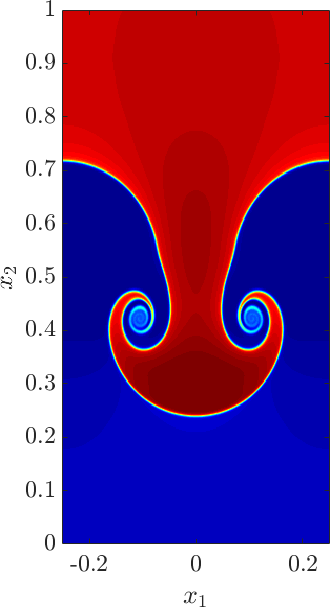
Figure 16: The density profile at time $t=2.5$ for the RTI test of Almgren et al. [1]. The solution is computed using the anisotropic $C$-method on a mesh with $128\times 512$ cells.

6.1.1.  The multiscale algorithm applied to the RTI

We next employ the RTI multiscale algorithm described in Section 5.3 with the following parameter values: the underlying coarse mesh used to solve for $v$ contains $8\times 32$ cells, while the interface is discretized with a fine mesh consisting of $N=128$ nodes; the time-step is $\delta t=2.5\times 10^{-3}$, giving $\mathrm{CFL}\approx 0.4$. The Atwood number is $A=1/3$, the initial velocity is $v_{0}=0$, the initial pressure is given by (51), the initial density is given by (52) with $h=0.02$, and

$$z_{1}(\alpha,0) =\alpha\,,$$

$$z_{2}(\alpha,0) =0.5-0.01\cos(4\pi\alpha)\,,$$

$$\varpi(\alpha,0) =0\,.$$

The artificial viscosity parameters are chosen as $\beta=50$, $\tilde{\delta}=1.0$, and $\mu=1.5\times 10^{-3}$.

We provide plots of the resulting solutions using our multiscale algorithm. The interface position $z$, at the final time $t=2.5$, is shown in Figure 17(a), and the high-resolution reference solution is shown in Figure 17(b). In Figure 17(c), we compare the interface positions computed using the multiscale algorithm and the high-resolution run; we see that the two solutions are in excellent agreement, with nearly identical spike tip and bubble tip positions; moreover, the multiscale algorithm successfully simulates the roll up of the vortex sheet. The reference solution computation had a runtime of $T_{\mathrm{CPU}}\approx 5015$ s, whereas the multiscale algorithm runtime was only $T_{\mathrm{CPU}}\approx 7$ s, giving a speed-up of approximately 683 times.

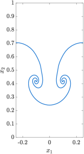
(a) Multiscale $z$

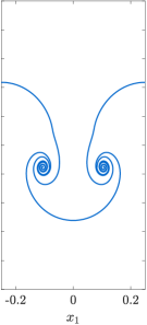
(b) High-res.

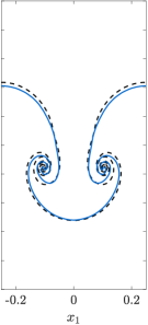
(c) Comparison

Figure 17: Results for the multiscale algorithm applied to the compressible single-mode RTI test of Almgren et al. [1], with the underlying grid containing $8\times 32$ cells and the interface discretized with $N=128$. Shown are (a) computed interface parametrization $z$, (b) benchmark interface position, and (c) the computed interface $z$ (blue) overlaying the benchmark solution (dashed black) at the final time $t=2.5$.

Increasing the resolution of both the coarse grid for $v$ and the fine grid for $w$ results in a solution with even more roll-up and accuracy. We show in Figure 18(a) the multiscale solution computed using $16\times 64$ cells for the coarse mesh and $N=256$ nodes for the fine mesh. The time-step is $\delta t\approx 8.333\times 10^{-4}$, giving $\mathrm{CFL}\approx 0.27$, and the artificial viscosity parameters are unchanged from the previous run. We observe that the computed interface shows more roll up, and is in even better agreement with the reference solution. The runtime of this simulation was $T_{\mathrm{CPU}}\approx 105$ s, resulting in a speed-up factor of approximately 48.

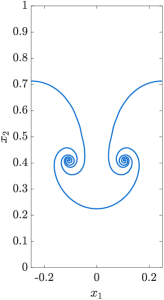
(a) Multiscale $z$

(b) High-res.

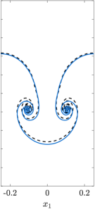
(c) Comparison

Figure 18: Results for the multiscale algorithm applied to the compressible single-mode RTI test of Almgren et al. [1], with the underlying grid containing $16\times 64$ cells and the interface discretized with $N=256$. Shown are (a) computed interface parametrization $z$, (b) benchmark interface position, and (c) the computed interface $z$ (blue) overlaying the benchmark solution (dashed black) at the final time $t=2.5$.

6.1.2.  Comparison of the low resolution density with the multiscale density

The multiscale algorithm solves for the velocity $v$ on a coarse mesh, using fine-scale information from the velocity $w$. In order to show how small-scale information improves the coarse-mesh simulation, we shall compare the solution obtained with our multiscale algorithm with the solution obtained by solving the Euler equations (using the same gas dynamics code as used for the high-resolution reference solution) on the same coarse meshes used to solve for $v$ in the multiscale algorithm. We shall refer to this gas dynamics simulation as the low resolution solution.

To be more precise, we obtain the low resolution density profile (using the $C$-method) on a grid with $16\times 64$ cells and with a time-step of $\delta t\approx 8.333\times 10^{-4}$. In Figure 19, this solution is compared against the multiscale density function obtained from the simulation shown in Figure 18. It is clear that the low resolution density profile does not have any of the basic KHI structure of the actual solution, and is very different from the multiscale density which (although solved for on the same coarse mesh) shows the KH roll-up structure. The multiscale algorithm allows for the recovery of small-scale information on the coarse grid via the computation of the velocity $w$ using a fine mesh for the interface. This small-scale information subsequently results in more structure in the roll-up region, and, therefore, a solution that is qualitatively more similar to high resolution simulations.

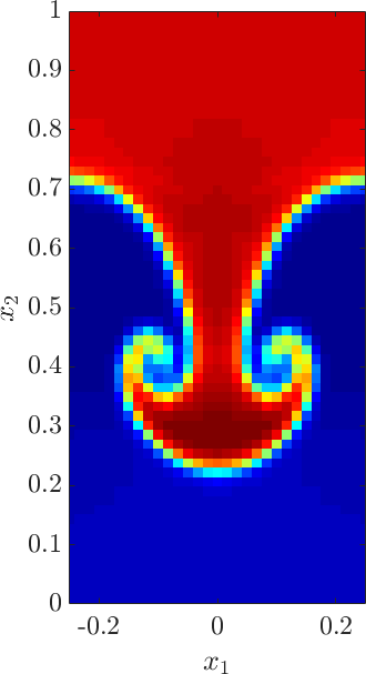
(a) Multiscale $\rho$

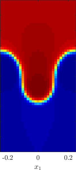
(b) Low-res. $\rho$

Figure 19: Comparison of the low resolution density with the multiscale density for the RTI test of Almgren et al. [1]. Figure 19(a) is a plot of the density computed using the multiscale algorithm, and Figure 19(b) is a plot of the low resolution Euler density, computed using the $C$-method on a coarse grid. Both solutions are computed using identical parameters.

6.1.3.   Comparison with other schemes and convergence studies

We next compare our multiscale algorithm with a modified version of the multiscale algorithm, in which the incompressible, irrotational velocity $w$ is computed using the kernels (34), rather than the Krasny kernel (30). As in Section 4.3, we are interested in the convergence properties of (1) the bubble and spike tip locations, and (2) the radius $r_{\delta}$ and location $\sigma_{\delta}$ of the spiral roll up region. We choose the axis $x_{2}=x_{2}^{*}=0.4125$ to compute the intersection points $x^{*}$.

We first take $N=128$ fixed and consider the limit $\delta\to 0$. The results are shown Figure 20. We observe that all three methods are in reasonable agreement with regards to the computed bubble and spike tip locations. The 3rd order kernel is in better agreement with the exact solution for the bubble position, whereas the Krasny kernel is in better agreement with the exact solution for the spike position. All three methods produce similar spiral radii $r_{\delta}$, and the computed values are in good agreement with the exact solution for $\delta>0$. The 3rd order kernel, in particular, is in excellent agreement with the exact solution. The spiral center locations are similarly reasonably accurate for $\delta>0$.

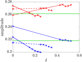
(a) Bubble (blue) and spike (red) tip locations.

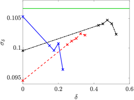
(b) Location of spiral center $\sigma_{\delta}$.

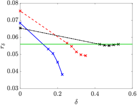
(c) Radius of spiral $r_{\delta}$.

Figure 20: Convergence behavior as $\delta\to 0$ with $N=128$ fixed for the compressible RTI test of Almgren et al. [1] using the $z$-model. Shown are (a) the bubble and spike tip locations, $|\max z_{2}-0.5|$ and $|\min z_{2}-0.5|$, respectively, (b) the location of the center of the spiral region $\sigma_{\delta}$, and (c) the radius of the spiral region $r_{\delta}$. The solid, dashed, and dotted curves in (a) refer to the Krasny, $\mathcal{K}^{\delta}_{1}$, and $\mathcal{K}^{\delta}_{3}$ kernels, respectively. The blue, red, and black curves in (b) and (c) refer to the Krasny, $\mathcal{K}^{\delta}_{1}$, and $\mathcal{K}^{\delta}_{3}$ kernels, respectively. The green curves indicate the corresponding quantities for the exact solution.

Next, we consider the limit $\delta,N^{-1}\to 0$. In particular, we consider $N=32,64,128,256$. We use the scaling (31) for the Krasny scheme, and the empirical procedure described at the beginning of Section 4.3 for the $\mathcal{K}^{\delta}_{i}$ kernel schemes. The results are shown in Figure 21. All of the schemes perform similarly, with the Krasny and $\mathcal{K}^{\delta}_{1}$ schemes in better agreement with the exact solution with regards to spike tip position, spiral center location $\sigma_{\delta}$, and spiral radius $r_{\delta}$, while the 3rd order kernel more accurately predicts the bubble tip location. We note that the convergence behavior of the 3rd order kernel scheme with regards to the quantities $\sigma_{\delta}$ and $r_{\delta}$ is rather erratic; this is a result of the sensitivity of the scheme to the choice of parameter $\delta$. The asymptotic behavior of $\sigma_{\delta}$ and $r_{\delta}$ in the Krasny scheme with the scaling (31), on the other hand, is more uniform.

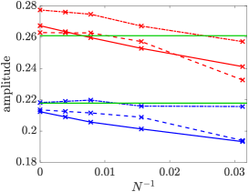
(a) Bubble (blue) and spike (red) tip locations.

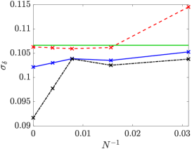
(b) Location of spiral center $\sigma_{\delta}$.

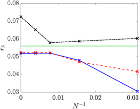
(c) Radius of spiral $r_{\delta}$.

Figure 21: Convergence behavior as $\delta,N^{-1}\to 0$ for the compressible RTI test of Almgren et al. [1] using the $z$-model. Shown are (a) the bubble and spike tip locations, $|\max z_{2}-0.5|$ and $|\min z_{2}-0.5|$, respectively, (b) the location of the center of the spiral region $\sigma_{\delta}$, and (c) the radius of the spiral region $r_{\delta}$. The solid, dashed, and dotted curves in (a) refer to the Krasny, $\mathcal{K}^{\delta}_{1}$, and $\mathcal{K}^{\delta}_{3}$ kernels, respectively. The blue, red, and black curves in (b) and (c) refer to the Krasny, $\mathcal{K}^{\delta}_{1}$, and $\mathcal{K}^{\delta}_{3}$ kernels, respectively. The green curves indicate the corresponding quantities for the exact solution.

6.2.  The compressible RTI test of Liska & Wendroff

For our next numerical experiment, we consider the compressible single-mode RTI from the review paper of Liska and Wendroff [62]. The domain is $(x_{1},x_{2})\in[-1/6,+1/6]\times[0,1]$, the gravitational constant is $g=0.1$, and the initial data is

$$\begin{bmatrix}\rho_{0}\\ (\rho u)_{0}\\ E_{0}\end{bmatrix}=\begin{bmatrix}1\\ 0\\ p_{0}/(\gamma-1)\end{bmatrix}\mathbbm{1}_{[0,\eta_{0})}(x_{2})+\begin{bmatrix}2\\ 0\\ p_{0}/(\gamma-1)\end{bmatrix}\mathbbm{1}_{[\eta_{0},1]}(x_{2})\,,$$ (53)

where the initial interface $\Gamma_{0}$ is parameterized by $(x_{1},\eta_{0}(x_{1}))$ with $\eta_{0}(x_{1})=0.5+0.01\cos(6\pi x_{1})$, and $p_{0}$ is the initial pressure, defined as

$$p_{0}=\begin{cases}2.4+g\,(\eta_{0}(x_{1})-x_{2})+2g\,(1-\eta_{0}(x_{1}))&,\text{ if }x_{2}<\eta_{0}(x_{1})\\ 2.4+2g\,(1-x_{2})&,\text{ if }x_{2}\geq\eta_{0}(x_{1})\\ \end{cases}\,,$$

Periodic conditions are applied in the horizontal direction $x_{1}$, while free-flow conditions are applied at the boundaries in the $x_{2}$ direction.

In [78], we used the anisotropic $C$-method to solve this problem; the resulting solutions have the classic mushroom-shaped interface profile without overly diffused KHI roll-up regions and mixing zones. We shall use this solution, computed on a fine mesh of $50\times 200$ cells with $\mathrm{CFL}\approx 0.1$ as our high resolution reference solution.

6.2.1.  The multiscale algorithm applied to the RTI

We begin by employing the multiscale algorithm to the RTI problem (53) with the following parameter values: the coarse mesh for $v$ contains $8\times 32$ cells, the fine mesh for $w$ uses $N=64$, and the time-step is $\delta t=2.5\times 10^{-3}$, giving $\mathrm{CFL}\approx 0.35$. The Atwood number is set as $A=1/3$, and the initial data is given by (53) (with $u$ replaced by $v$) with the following modification: as in the numerical experiment performed in Section 6.1, we smooth the initial density field $\rho_{0}$ over a length scale. The initial density is thus given by formula (52) with $\eta_{0}(x_{1})=0.5+0.01\cos(6\pi x_{1})$, and the smoothing length scale is chosen as $h=0.02$. We also set

$$z_{1}(\alpha,0) =\alpha\,,$$

$$z_{2}(\alpha,0) =0.5+0.01\cos(6\pi\alpha)\,,$$

$$\varpi(\alpha,0) =0\,.$$

The artificial viscosity parameters are chosen as $\beta=5$, $\tilde{\delta}=1.5$, and ${\mu}=0.001$.

The multiscale interface position $z$ at time $t=8.5$ is shown in Figure 22; the high resolution reference solution computation is presented in Figure 22(b), and the comparison of the two solution is made in Figure 22(c). We see that the spike tip position of the computed solution matches almost exactly with the spike tip position of the reference solution, and the bubble tip positions are also in good agreement. Moreover, the multiscale solution successfully simulates the roll-up of the contact discontinuity and, by comparing with Figure 22(b), we observe that this roll-up occurs in the correct region of the flow and matches well with the scale of the high resolution solution.

In Figure 23, we compare the interface $z(\alpha,t)$ from the multiscale run and the high-resolution run at various times $t$. As can be seen, the two solutions are in very good agreement throughout the time interval of the simulation.

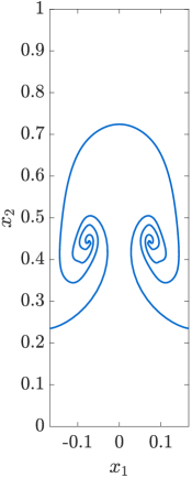
(a) Multiscale $z$

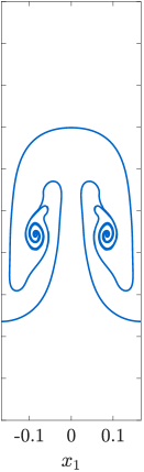
(b) High-res.

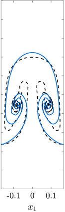
(c) Comparison

Figure 22: Results for the multiscale algorithm applied to the compressible single-mode RTI test of Liska and Wendroff [62], with the underlying grid containing $8\times 32$ cells and the interface discretized with $N=64$. Shown are (a) computed interface parametrization $z$, (b) benchmark interface position, and (c) the computed interface $z$ (blue) overlaying the benchmark solution (dashed black) at the final time $t=8.5$.

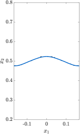
(a) $t=2.0$

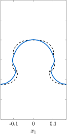
(b) $t=5.0$

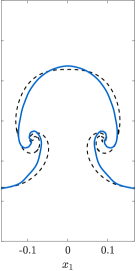
(c) $t=6.0$

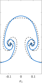
(d) $t=7.0$

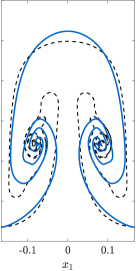
(e) $t=8.5$

Figure 23: Evolution over time $t$ of the interface for the compressible single-mode RTI. Here $z$ is computed using the multiscale algorithm on a mesh with $8\times 32$ cells and an interface discretized with $N=64$. The blue curve is the computed $z(\alpha,t)$, and the dashed black curve is the reference solution.

To compare the bubble and spike tip positions, we plot in Figure 24 the quantities $\sigma_{b}(t)=|0.5-\max_{\alpha}z(\alpha,t)|$ and $\sigma_{s}(t)=|0.5-\min_{\alpha}z(\alpha,t)|$. The spike tip position is in excellent agreement with the reference solution for all times $t$, while the bubble tip position is also in excellent agreement for times $t<6$. For $t>6$, the bubble tip position diverges slightly from the reference solution, but the error is still relatively small; at the final time $t=8.5$, the error is $\approx 2.5\%$ of the height of the computational domain.

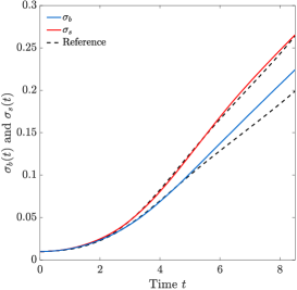
Figure 24: Plots of the quantities $\sigma_{b}(t)$ and $\sigma_{s}(t)$ for the solution computed using the multiscale algorithm applied to the compressible single-mode RTI on a mesh with $8\times 32$ cells and an interface with $N=64$.

Finally, we turn to the issue of the runtimes of the computations. The reference solution computation had a runtime of $T_{\mathrm{CPU}}\approx 2906$ s, whereas the multiscale algorithm runtime was only $T_{\mathrm{CPU}}\approx 14$ s, which gives a speed-up of approximately 203 times. We are thus able to infer both large-scale (amplitude growth rates) as well as small-scale (roll-up region structure) information by use of the multiscale model and algorithm, while drastically reducing the computational burden and runtime when compared with the reference solution computation.

6.2.2.  Comparing the mutliscale solution with both the low resolution simulation and the incompressible $z$-model

To demonstrate the efficacy of our multiscale model, we compare the multiscale solution with the low resolution solution as well as with the incompressible and irrotational $z$-model.

In Figure 25, the results from these simulations are compared with the simulations performed using the multiscale algorithm. We see that the solutions are drastically different; the low resolution density $\rho$ has no roll-up of the contact discontinuity, while the interface $z$ computed using the incompressible $z$-model has completely incorrect bubble and spike positions. On the other hand, the use of the multiscale model allows the coarse grid calculation to “correct” the interface position $z$, while the fine resolution computation on the interface $z$ similarly “corrects” for the lack of roll-up of the coarse grid solution.

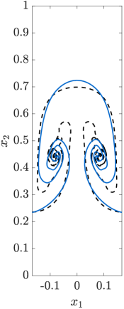
(a) Multiscale $z$

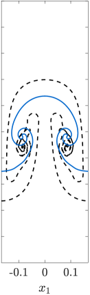
(b) $z$-model

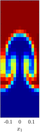
(c) Multiscale $\rho$

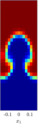
(d) Low res. $\rho$

Figure 25: Comparison of the solutions to the compressible single-mode RTI test of Liska and Wendroff [62]. Figures 25(a) and 25(c) are plots of the interface $z$ and density $\rho$, respectively, computed using the multiscale algorithm. Figure 25(b) is the interface $z$ computed using the incompressible and $z$-model. Figure 25(d) is the low resolution density $\rho$ computed using the $C$-method. All the relevant parameters are fixed across the simulations.

6.2.3.  Basic mesh refinement study

Next, we perform a basic mesh refinement study to analyze the behavior of our multiscale algorithm as both the underlying mesh, as well as the interface discretization, is refined. More precisely, we shall consider grids with $8\times 32$, or $10\times 40$ or $12\times 48$ cells, and the interface discretized with either $N=64$ or $N=128$ or $N=256$. We shall keep the artificial viscosity parameters $\beta$ and $\tilde{\delta}$ fixed, with $\beta=5$ and $\tilde{\delta}=1.5$. The time-step $\delta t$ and artificial viscosity parameter ${\mu}$ are allowed to vary as both the underlying mesh resolution, as well as the interface resolution, are varied. The exact choices for these parameters, as well as the corresponding runtimes $T_{\mathrm{CPU}}$ and speed-up factors $\Lambda$ compared to the high resolution reference solution calculation, are presented in Table 3 in Appendix A, but we note here that the values of ${\mu}$ are almost the same (${\mu}\approx 0.001$) for all of the runs.

The results for the mesh refinement study are shown in Figure 34 in Appendix A. As $N$ increases with the number of cells fixed, the computed interface positions are roughly the same, except in the KHI roll-up regions, in which the interfaces computed with larger $N$ show significantly more roll-up (compare, for instance, Figure 34(a) with Figure 34(c)). This is in line with the observations in Section 4.3 for numerical simulations using the incompressible and irrotational $z$-model, and is due to the scaling of the parameter $\tilde{\delta}$.

On the other hand, if the number of cells contained in the underlying coarse mesh is increased with $N$ held fixed, the resulting solutions for the interface do not have more roll-up, but instead appear to converge to the reference solution away from the roll-up region (compare, for instance, Figure 34(b) with Figure 34(h)). This “convergence” is particularly noticeable in the “pits” of the mushroom shape.

6.3.  A single-mode RMI problem

We next consider the single-mode RMI with the following problem setup. The domain is $(x_{1},x_{2})\in[-1/6,+1/6]\times[-1,1]$, the gravitational constant is $g=0.5$, and the initial data is given by

$$\begin{bmatrix}\rho_{0}\\ (\rho u)_{0}\\ E_{0}\end{bmatrix}=\begin{bmatrix}1\\ 0\\ f/(\gamma-1)\end{bmatrix}\mathbbm{1}_{[-1,\eta_{0})}(x_{2})+\begin{bmatrix}2\\ 0\\ f/(\gamma-1)\end{bmatrix}\mathbbm{1}_{[\eta_{0},0.8)}(x_{2})+\begin{bmatrix}4.857143\\ 0\\ 36.6666+f/(\gamma-1)\end{bmatrix}\mathbbm{1}_{[0.8,1]}(x_{2})\,,$$ (54)

where the initial interface $\Gamma_{0}$ is parameterized by $(x_{1},\eta_{0}(x_{1}))$ with $\eta_{0}(x_{1})=0.5+0.1\cos(6\pi x_{1})$, and $f$ is the function defined as

$$f(x_{1},x_{2})=\begin{cases}2.4+g\,(\eta_{0}(x_{1})-x_{2})+2g\,(1-\eta_{0}(x_{1}))&,\text{ if }x_{2}<\eta_{0}(x_{1})\\ 2.4+2g\,(1-x_{2})&,\text{ if }x_{2}\geq\eta_{0}(x_{1})\\ \end{cases}\,,$$

Periodic conditions are applied in the horizontal direction $x_{1}$, while free-flow and solid-wall conditions are applied at the bottom and top boundaries, respectively.

A high resolution reference solution is computed using the $C$-method on a fine grid with $50\times 400$ cells. The time-step is fixed as $\delta t=0.0001$, which results in $\mathrm{CFL}\in(0.14,0.2)$. Again, we have found that this relatively small CFL number is required to prevent the occurrence of high-frequency noise in the computed solution.

6.3.1.  The multiscale algorithm applied to the RMI

We apply the multiscale algorithm to the RMI problem (54) with the following parameter choices: the coarse mesh for $v$ contains $10\times 80$ cells, the fine mesh for $w$ uses $N=64$, and the time-step is $\delta t=0.00125$, which yields $\mathrm{CFL}\in(0.30,0.45)$. The artificial viscosity parameters in (59) are set as $\beta=1$, $\beta_{s}=1$, while $\tilde{\delta}=1.25$ and ${\mu}=0.005$. The Atwood number is set as $A=1/3$, and the initial data is given by (54) (with $u$ replaced by $v$), together with

$$z_{1}(\alpha,0) =\alpha\,,$$

$$z_{2}(\alpha,0) =0.5+0.1\cos(6\pi\alpha)\,,$$

$$\varpi(\alpha,0) =0\,.$$

We present results for the computed interface parametrization at the final time $t=1.6$ in Figure 26(a). Plots showing the evolution of the interface over time are shown in Figure 27. The computed interface position $z$ agrees well with the reference solution for the duration of simulation, and both interfaces display similar amounts of roll-up at the final time.The positions of the bubbles coincide for the two solution, while the spike tip positions are also in good agreement. We also note that in the high resolution reference solution there is slight “kink” in the “stem” of the mushroom; this “kink” is also displayed in the interface computed using the multiscale algorithm.

The approximate runtime of the reference solution calculation is $T_{\mathrm{CPU}}\approx 1653$ s, whereas our multiscale algorithm computation had a runtime of only $T_{\mathrm{CPU}}\approx 15$ s, yielding a speed-up factor of almost 110 times. As with the multiscale algorithm applied to the RTI, we are able to accurately predict large scale quantities and small scale structure with minimal computational expense.

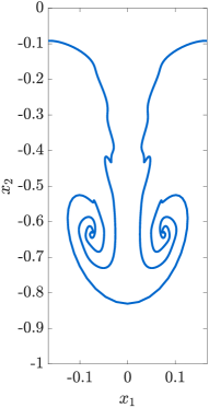
(a) Multiscale $z$

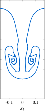
(b) High-res.

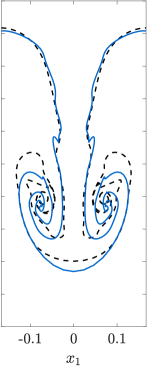
(c) Comparison

Figure 26: Results for the multiscale algorithm applied to single-mode RMI test, with the underlying grid containing $10\times 80$ cells and the interface discretized with $N=64$. Shown are (a) computed interface parametrization $z$, (b) benchmark interface position, and (c) the computed interface $z$ (blue) overlaying the benchmark solution (dashed black) at the final time $t=1.6$.

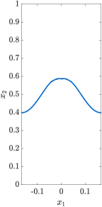
(a) $t=0.1$

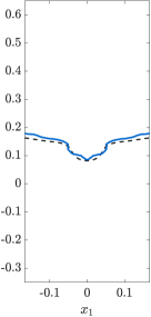
(b) $t=0.4$

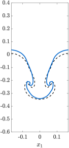
(c) $t=0.8$

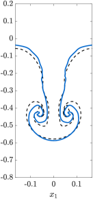
(d) $t=1.2$

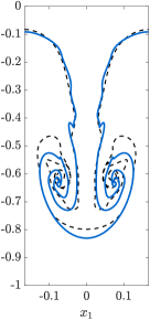
(e) $t=1.6$

Figure 27: Evolution over time $t$ of the interface for the single-mode RMI. Here $z$ is computed using the multiscale algorithm on a mesh with $10\times 80$ cells and an interface discretized with $N=64$. The blue curve is the computed $z(\alpha,t)$, and the dashed black curve is the reference solution.

6.3.2.  The effects of the baroclinic term

In this section, we briefly discuss the importance of including the baroclinic term in the modified $\varpi$-equation (47b). This term is crucial in ensuring that the interface $z$ is advected by the correct velocity. Without this term, information about the baroclinic deposition of vorticity by the shock on the interface is not transmitted to the incompressible portion of the multiscale algorithm. We show in Figure 28 the evolution of a multiscale solution, computed without the inclusion of the baroclinic term, but otherwise identical to the RMI multiscale algorithm. This solution (displayed as a red curve) is compared against the solution obtained using the actual RMI multiscale algorithm (displayed as a blue curve), as well as the high resolution reference solution (displayed as a dashed black curve). It is clear that the omission of the baroclinic term leads to a solution with an incorrect interface position, and with significantly less KH roll-up.

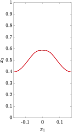
(a) $t=0.1$

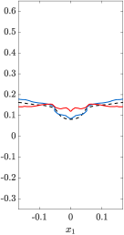
(b) $t=0.4$

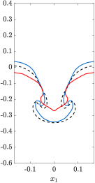
(c) $t=0.8$

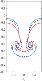
(d) $t=1.2$

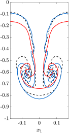
(e) $t=1.6$

Figure 28: Evolution over time $t$ of the interface for the single-mode RMI. Here, the red curve is $z$ computed using the multiscale algorithm, but without the use of the baroclinic term in the $\varpi$-equation, on a mesh with $10\times 80$ cells and an interface discretized with $N=64$. The blue curve is $z$ computed using the complete multiscale algorithm, while dashed black curve is the reference solution.

In the absence of this baroclinic term, while the coarse scale shock velocity $v$ still advects the interface upon shock-contact collision, the computed amplitude of vorticity $\varpi$ (shown in Figure 29 as a red curve) has the wrong sign after the shock-contact collision at $t\approx 0.12$, which yields an incorrect calculation of the fine scale velocity $w$, and subsequently an incorrect interface position $z$.

We compare this incorrect $\varpi$ with the amplitude of vorticity $\varpi$ computed using the complete RMI multiscale algorithm (shown in Figure 29 as a blue curve); without the baroclinic term, $\varpi$ has the wrong sign until time $t=0.70$, at which point the advection of the interface by the coarse scale velocity $v$ forces $\varpi$ to have the correct sign. This is in contrast to our RMI multiscale algorithm, in which the baroclinic term forces $\varpi$ to switch sign after the shock-contact interaction, which results in the correct computation of the fine grid velocity $w$ and, consequently, the correct interface position.

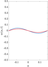
(a) $t=0.05$

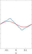
(b) $t=0.10$

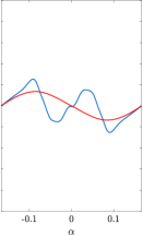
(c) $t=0.12$

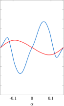
(d) $t=0.15$

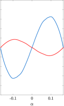
(e) $t=0.20$

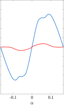
(f) $t=0.70$

Figure 29: Evolution over time $t$ of the amplitude of vorticity $\varpi(\alpha,t)$ versus $\alpha$ for the single-mode RMI. Here, the red curve is $\varpi$ computed using the multiscale algorithm, but without the use of the baroclinic term in the $\varpi$-equation, on a mesh with $10\times 80$ cells and an interface discretized with $N=64$. The blue curve is $\varpi$ computed using the complete multiscale algorithm.

6.4.  The RMI test of Nourgaliev et al.

We next consider the RMI problem introduced in [75], and later considered in [97, 74, 105]. A heavy fluid of density $\rho^{+}=5.04$ lies below a light fluid of density $\rho^{-}=1$, and a planar Mach 1.24 shock travels vertically downards through the light fluid and eventually collides with the interface separating the two fluids, resulting in a transmitted shock and a reflected shock. The instability is generated by the subsequent acceleration of the light fluid into the heavy fluid. The domain is $(x_{1},x_{2})\in[-0.5,0.5]\times[0,4]$, the adiabatic constant is $\gamma=1.276$, gravity is assumed to be negligible (i.e. $g=0$), and the initial data is defined as follows. The initial interface $\Gamma_{0}$ is parametrized by $(x_{1},\eta_{0}(x_{1}))$, with $\eta_{0}(x_{1})=2.9+0.1\cos(2\pi x_{1})$, and the initial shock position is at $x_{2}=3.2$. The initial horizontal velocity vanishes $u_{1}(x,0)=0$, and the initial vertical velocity satisfies $u_{2}(x,0)=-0.550368\cdot\mathbbm{1}_{x_{2}\geq 3.2}(x)$. The initial pressure is $p_{0}(x)=\mathbbm{1}_{x_{2}<3.2}(x)+1.628\cdot\mathbbm{1}_{x_{2}\geq 3.2}(x)$. As in the numerical experiments in Section 6.1, the initial density is smoothed over a length scale $h$ using a $\tanh$ profile:

$$\rho_{0}(x_{1},x_{2})=\rho^{-}+\frac{\rho^{+}-\rho^{-}}{2}\left[1+\tanh\left(\frac{\psi(x_{1})-x_{2}}{h}\right)\right]\,.$$ (55)

For our high resolution reference solution computed using the $C$-method on a fine mesh, we use $h=0.005$. Periodic boundary conditions are applied in the $x_{1}$-direction, and free-flow conditions are imposed in the $x_{2}$-direction.

Our high resolution reference solution is computed on a mesh with $100\times 800$ cells and a time-step of $\delta t=6.25\times 10^{-4}$, which gives $\mathrm{CFL}\approx 0.4$. The computed density is shown in Figure 30 at the final time $t=8$, and can be compared with Figures 10, 11, 23, and 23 in [75], [97], [74], and [105], respectively.

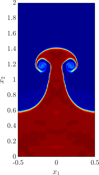
Figure 30: The density profile at time $t=8.0$ for the RMI test of Nourgaliev et al. [75]. This high-resolution solution is computed using the $C$-method on a mesh with $100\times 800$ cells.

6.4.1.  The multiscale algorithm applied to the RMI

Next, we apply the multiscale RMI algorithm to the problem described above. The relevant parameters are chosen as follows. The coarse mesh for $v$ contains $10\times 80$ cells, the fine mesh for $w$ uses $N=128$, and the time-step is set as $\delta t=6.25\times 10^{-3}$, giving $\mathrm{CFL}\approx 0.4$. The initial velocities are $v_{1}(x,0)=0$ and $v_{2}(x,0)=-0.550368\cdot\mathbbm{1}_{x_{2}\geq 3.2}(x)$, and the initial pressure is $p_{0}(x)=\mathbbm{1}_{x_{2}<3.2}(x)+1.628\cdot\mathbbm{1}_{x_{2}\geq 3.2}(x)$. The initial density is smoothed using (55) with $h=0.02$. The Atwood number is $A\approx 0.67$, and the initial data for the interface calculation is

$$z_{1}(\alpha,0) =\alpha\,,$$

$$z_{2}(\alpha,0) =2.9+0.1\cos(2\pi\alpha)\,,$$

$$\varpi(\alpha,0) =0\,.$$

The artificial viscosity parameters are set as $\beta=1$, $\beta_{s}=0$, $\tilde{\delta}=1$, and $\varpi=1\times 10^{-4}$.

The computed interface is shown in Figure 31(a), the high resolution reference solution is shown in Figure 31(b), and a comparison of the two solutions is made in Figure 31(c). The multiscale algorithm is able to simulate both the transport of the contact as well as the KHI roll up; moreover, Figure 31(c) shows that the bubble tip and spike tip positions compare well with the high resolution reference solution. The runtime for the high resolution simulation was $T_{\mathrm{CPU}}\approx 6298$ s, whereas the runtime for the multiscale simulation was only $T_{\mathrm{CPU}}\approx 24$ s, giving a speed up factor of approximately 260 times.

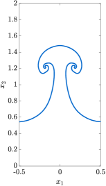
(a) Multiscale $z$

(b) High-res.

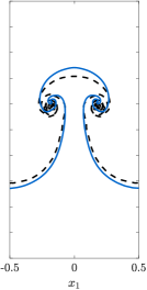
(c) Comparison

Figure 31: Results for the multiscale algorithm applied to single-mode RMI test of Nourgaliev et al. [75], with the underlying grid containing $10\times 80$ cells and the interface discretized with $N=128$. Shown are (a) computed interface parametrization $z$, (b) benchmark interface position, and (c) the computed interface $z$ (blue) overlaying the benchmark solution (dashed black) at the final time $t=8.0$.

Next, we double the resolution of both the coarse mesh for $v$ as well as the fine mesh for $w$ i.e. the grid now contains $20\times 160$ cells and $N=256$. The time-step is halved, $\delta t=3.125\times 10^{-3}$, so that the CFL number is still approximately 0.4. All the other parameters from the previous run are kept fixed, and we employ the multiscale algorithm; the resulting solution is shown in Figure 32(a). We see that there is more roll-up of the vortex sheet, and that the “cap” of the mushroom is “flattened”, which is in qualitative agreement with the reference solution. The runtime for this simulation is $T_{\mathrm{CPU}}\approx 265$ s, giving a speed up factor of approximately 24 times over the high resolution simulation.

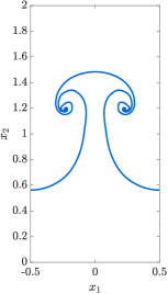
(a) Multiscale $z$

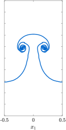
(b) High-res.

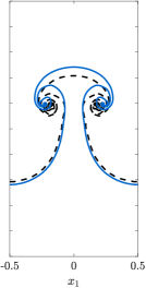
(c) Comparison

Figure 32: Results for the multiscale algorithm applied to single-mode RMI test of Nourgaliev et al. [75], with the underlying grid containing $20\times 160$ cells and the interface discretized with $N=256$. Shown are (a) computed interface parametrization $z$, (b) benchmark interface position, and (c) the computed interface $z$ (blue) overlaying the benchmark solution (dashed black) at the final time $t=8.0$.

6.4.2.  The effects of the Taylor hypothesis

We now briefly discuss the effects of the Taylor "frozen turbulence" hypothesis in our multiscale RMI algorithm. We recall that the hypothesis asserts that the fine grid velocity $w$ is transported by the coarse grid velocity $v$ (over small time intervals). The primary effect of the Taylor hypothesis is that the dynamics of the coarse grid compressible velocity $v$ are evolved using (28b’) in place of (28b). Without the use of the hypothesis, the additional terms in (28b) lead to an incorrect calculation of the velocity field $v$, which in turn leads to an incorrect update of the interface position $z$ (i.e. Steps Step 11(e), Step 11(f) and Step 44(b), Step 44(c) of the RMI algorithm).

We demonstrate this in Figure 33, in which we show results of a simulation performed using a modified version of the RMI multiscale algorithm in which the Taylor hypothesis is not employed, but is otherwise identical to the RMI multiscale algorithm in Section 5.3. The solution is computed using the same parameters as those used for the simulation presented in Figure 31(a).

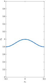
(a) $t=0.15$

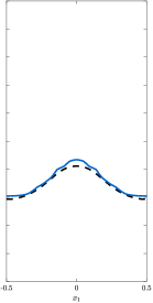
(b) $t=1.0$

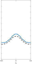
(c) $t=1.25$

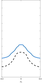
(d) $t=2.0$

Figure 33: Results for the modified multiscale algorithm without the Taylor “frozen turbulence” hypothesis applied to single-mode RMI test of Nourgaliev et al. [75], with all relevant parameters unchanged from the simulation presented in Figure 31. Shown are the computed interface $z$ (blue) and reference solution (dashed black) at various times $t$.

The shock collides with the interface at time $t=0.15$, shown in Figure 33(a); at this time, vorticity is deposited on the interface by the shock. The interface is transported with reasonable accuracy for $t<1.0$ (as demonstrated in Figure 33(b)), because the velocity $w$ is very small at early times, and thus does not have a noticeable effect on the interface evolution; for early times, the evolution of the interface is mainly due to the “transport” coarse grid velocity $v$. However, as the magnitude of the vorticity on the interface grows with time, $w$ is no longer negligible, and affects the evolution of the interface. The extra terms appearing on the right-hand side of (28b) (which do not appear in (28b’)) lead to an incorrect calculation of the coarse scale velocity $v$. Since the fine grid velocity $w$ is not being transported by $v$, the coarse scale compression and vorticity information is not correctly conveyed to the interfacial algorithm, which leads to a deceleration of the interface (shown in Figure 33(c)). The solution then quickly degrades, with the interface position completely incorrect by time $t=2.0$, as shown in Figure 33(d). For problems in which an unstable interface is transported as the instability develops, the use of the Taylor hypothesis ensures that coarse scale information is accurately conveyed to the small scale calculations, thereby producing accurate solutions with correct interface positions.

7.  Concluding remarks

This paper introduces a novel multiscale model describing the evolution of contact discontinuities in compressible fluid flow. The multiscale model is based on a decomposition of the velocity field $u=v+w$. While the velocity $w$ is discontinuous, it is also incompressible and irrotational, and can be solved efficiently on fine meshes using a new asymptotic (high-order) $z$-model to approximate the full Birkhoff-Rott system of singular integral equations. The velocity $v$ is compressible and rotational, but is smooth near the contact discontinuity and can thus be computed efficiently on relatively coarse meshes.

We have proposed an extremely simple numerical implementation of the incompressible $z$-model, and have presented numerical results for the $z$-model which simulate classical RTI experiments. These results show excellent qualitative and quantitative agreement of our computed solutions with both experimental predictions, as well as “reference” solution calculations performed using the complete Birkhoff-Rott system. In the latter case, we have demonstrated that our $z$-model algorithm is at least 75 times faster than a standard numerical algorithm for the Birkhoff-Rott system. We have additionally compared our simple numerical implementation with more sophisticated methods using higher order regularizations, and found good agreement (as in previous numerical studies [8, 93]) between all three methods in predicting both the bubble and spike tip locations, as well as the radii and location of the spiral roll up structures. While our simple numerical method leads to a fast-running algorithm, in the future, more sophisticated numerical implementations of the $z$-model will be considered, including implementations of a fast summation method [45], a point-insertion procedure [57], non-oscillatory shock-capturing, and space-time smooth artificial viscosity [77].

We have also developed multiscale models and algorithms for compressible flows with vorticity undergoing RTI and RMI. Our algorithms couple the fine scale velocity $w$, which controls the small scale structure of the interface, with the coarse grid velocity $v$, which controls the bulk compression and vorticity of the fluid. The RMI multiscale algorithm includes the effects of vorticity deposition on the interface during shock-contact interaction, and also enforces a version of Taylor’s frozen turbulence hypothesis, which asserts that small scale velocity fluctuations are transported by the mean flow. We have presented numerical results for both the RTI and RMI, and demonstrated that the computed solutions are in good agreement, both qualitatively and quantitively, with high order gas dynamics simulations, while having computational run times that are at least two orders of magnitude smaller. In particular, the multiscale solutions exhibit KHI roll up regions of the contact discontinuity that are in good agreement with the roll up regions observed in solutions obtained from high resolution calculations. Such roll up of the contact is in general not observed in low resolution Euler simulations; however, the coupling of the fine scale velocity $w$ to the coarse scale velocity $v$ through our multiscale model leads to simulations (on coarse meshes) which exhibit roll-up regions similar to those in high-resolution simulations.

In future work, we shall generalize our models to three space dimensions, and consider its applications to the numerical simulation of other physical problems, such as RTI and RMI with multimode initial perturbations, rising bubbles, and shock-bubble interaction. The mathematical analysis of the $z$-model and the multiscale models will also be considered in future work. In particular, we shall consider a detailed theoretical and numerical study of the convergence behavior of our multiscale solutions, as the interfacial and planar meshes are refined, and artificial viscosity parameters converge to zero.

Acknowledgements

SS was partially supported by DTRA HDTRA11810022. We would like to express our gratitude to the anonymous referee for their numerous suggestions that have greatly improved the manuscript.

Appendix A Mesh refinement for the multiscale algorithm applied to the RTI

In this section, we present the results for the mesh refinement study of the multiscale algorithm applied to the single-mode compressible RTI test of Liska & Wendroff (see Section 6.2.3). Table 3 contains a list of the choices for the parameters $\delta t$ and $\mu$, as well as the runtimes $T_{\mathrm{CPU}}$ and relative speed up factors $\Lambda$ for the RTI mesh refinement study. The results from this study are presented in Figure 34, which show the reference solution (dashed black curve) overlaid by the computed interface parametrization $z$ (red curve).

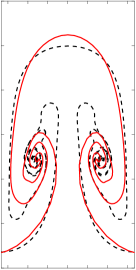
(a) $8\times 32$, $N=64$

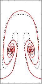
(b) $8\times 32$, $N=128$

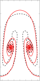
(c) $8\times 32$, $N=256$

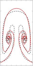
(d) $10\times 40$, $N=64$

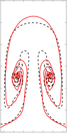
(e) $10\times 40$, $N=128$

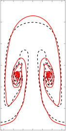
(f) $10\times 40$, $N=256$

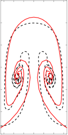
(g) $12\times 48$, $N=64$

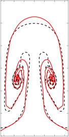
(h) $12\times 48$, $N=128$

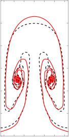
(i) $12\times 48$, $N=256$

Figure 34: Plots of the interface computed using the multiscale algorithm applied to the single-mode compressible RTI test of Liska and Wendroff [62] for different grid and interface resolutions. The red curve is the computed interface, and the dashed black curve is the reference solution.

	64	128	256
$8\times 32$	$\delta t=2.5\times 10^{-3}$	$\delta t=2.5\times 10^{-3}$	$\delta t=6.25\times 10^{-4}$
	${\mu}=1\times 10^{-3}$	${\mu}=9\times 10^{-4}$	${\mu}=8.75\times 10^{-4}$
	$T_{\mathrm{CPU}}=14$ s	$T_{\mathrm{CPU}}=28$ s	$T_{\mathrm{CPU}}=244$ s
	$\Lambda=203$	$\Lambda=105$	$\Lambda=12$
$10\times 40$	$\delta t=2.5\times 10^{-3}$	$\delta t=2.5\times 10^{-3}$	$\delta t=6.25\times 10^{-4}$
	${\mu}=1\times 10^{-3}$	${\mu}=8.75\times 10^{-4}$	${\mu}=9\times 10^{-4}$
	$T_{\mathrm{CPU}}=19$ s	$T_{\mathrm{CPU}}=37$ s	$T_{\mathrm{CPU}}=304$ s
	$\Lambda=149$	$\Lambda=78$	$\Lambda=10$
$12\times 48$	$\delta t=1.67\times 10^{-3}$	$\delta t=1.67\times 10^{-3}$	$\delta t=4.55\times 10^{-4}$
	${\mu}=1.5\times 10^{-3}$	${\mu}=1.25\times 10^{-3}$	${\mu}=1.1\times 10^{-3}$
	$T_{\mathrm{CPU}}=38$ s	$T_{\mathrm{CPU}}=69$ s	$T_{\mathrm{CPU}}=578$ s
	$\Lambda=76$	$\Lambda=42$	$\Lambda=5$

Table 3: Time-step $\delta t$ and artificial viscosity parameter ${\mu}$ choices for the compressible single-mode RTI mesh refinement study described in Section 6.2.3. Shown also are the runtimes $T_{\mathrm{CPU}}$ and speed-up factors $\Lambda$.

Appendix B The $C$-method for space-time smooth artificial viscosity

The presence of jump discontinuities in the solution $\bf{U}$ to (10) poses a significant challenge for numerical schemes attempting to approximate such solutions, due to the occurrence of small-scale oscillations (or Gibbs phenomenon). A variety of high-order discretization techniques have been developed to combat this issue, such as MUSCL [101, 24, 52], PPM [25], WENO [64, 53, 86], and its predecessor, ENO [49, 87, 88]. These methods rely on a careful reconstruction of the numerical flux; centered numerical fluxes, such as the Lax-Friedrichs flux [60], add dissipation implicitly to preserve stability and monotonicity, while upwinding methods based upon exact or approximate Riemann solvers tend to be complex and computationally costly. We refer the reader to [77] and the references therein for further details.

Explicit artificial viscosity methods provide a simple way to stabilize shock fronts and contact discontinuities. These methods regularize solutions by introducing diffusion terms to the equations of motion; discontinuities are smeared over a small region in space, which stabilize the solution and prevent the occurrence of spurious oscillations, while high-order accuracy is maintained in smooth regions of the flow. We next describe a method for adding localized, space-time smooth artificial viscosity to the system (10), which we call the $C$-method [80, 77, 78].

The $C$-method is a variant of the original classical artificial viscosity method of Von Neumann and Richtmyer [103], and couples the Euler equations (10) to a set of scalar reaction-diffusion equations, whose solutions act as space-time smooth artificial viscosity indicators. The $C$-method tracks the geometry of the evolving fronts, which allows for the implementation of both directionally isotropic and anisotropic artificial viscosity schemes. The latter is important for the capture of the roll-up of vortex sheets subject to the Kelvin-Helmholtz instability.

We introduce the following Euler-$C$-$\hat{C}$ system:

$$\partial_{t}\rho+\nabla\cdot(\rho u) =0\,,$$ (56a)

$$\partial_{t}(\rho u)+\nabla\cdot(\rho u\otimes u)+\nabla p+\rho ge_{2} =\partial_{x_{i}}\left(\tilde{\beta}\rho\hat{C}C^{\tau_{i}}C^{\tau_{j}}\partial_{x_{j}}u\right)+\nabla\cdot(\tilde{\beta_{s}}\rho C\nabla u)\,,$$ (56b)

$$\partial_{t}E+\nabla\cdot(u(E+p))+\rho gu_{2} =0\,,$$ (56c)

$$\partial_{t}C-\mathscr{L}[C\,;\varepsilon,\kappa] =\frac{S(u)}{\varepsilon|\delta x|}G_{\rho}\,,$$ (56d)

$$\partial_{t}\hat{C}-\mathscr{L}[\hat{C}\,;\varepsilon,\kappa] =\frac{S(u)}{\varepsilon|\delta x|}\hat{G}_{\rho}\,,$$ (56e)

$$\partial_{t}C^{\tau_{i}}-\mathscr{L}[C^{\tau_{i}}\,;\varepsilon,\kappa] =\frac{S(u)}{\varepsilon|\delta x|}\hat{\tau}_{i}\,,\text{ for }i=1,2\,.$$ (56f)

Here, the operator $\mathscr{L}$ is defined by

$$\mathscr{L}[C\,;\varepsilon,\kappa]=-\frac{S(u)}{\varepsilon|\delta x|}C+\kappa S(u)\Delta C\,,$$ (57)

where $\varepsilon$ and $\kappa$ are parameters controlling the support and smoothness of the function $C$, respectively, $\delta x=(\delta x_{1}\,,\delta x_{2})$ is the grid spacing, and $\Delta=\partial_{x_{1}}^{2}+\partial_{x_{2}}^{2}$ is the Laplacian operator. The forcing functions to the $C$-equations are

$$G_{\rho} =\mathbbm{1}_{(-\infty,0)}(\nabla\cdot u)[1-\mathbbm{1}_{(\infty,0)}(\partial_{n}\rho\partial_{n}e)]|\nabla\rho|\,,$$ (58a)

$$\hat{G}_{\rho} =\mathbbm{1}_{(-\infty,0)}(\partial_{n}\rho\partial_{n}e)|\nabla\rho|\,,$$ (58b)

$$\hat{\tau}_{1} =-\mathbbm{1}_{(-\infty,0)}(\partial_{n}\rho\partial_{n}e)\partial_{y}\rho\,,$$ (58c)

$$\hat{\tau}_{2} =\mathbbm{1}_{(-\infty,0)}(\partial_{n}\rho\partial_{n}e)\partial_{x}\rho\,,$$ (58d)

where $\partial_{n}=n\cdot\nabla$ is the normal derivative operator and the function $\mathbbm{1}_{(-\infty,0)}(\xi)$ is a compression or expansion switch defined by

$$\mathbbm{1}_{(-\infty,0)}(\xi)=\begin{cases}1\,,&\text{if }\xi<0\,,\\ 0\,,&\text{if }\xi\geq 0\,.\end{cases}$$

The artificial viscosity parameters $\tilde{\beta}$ and $\tilde{\alpha}$ are defined by

$$\tilde{\beta}=|\delta x|^{2}\cdot\frac{\max_{x}|\nabla u|}{\mu^{2}\max_{x}\hat{C}}\beta\quad\text{ and }\quad\tilde{\beta_{s}}=|\delta x|^{2}\cdot\frac{\max_{x}|\nabla u|}{\max_{x}C}\beta_{s}\,,$$ (59)

with $\mu=\max_{x}\left\{|C^{\tau_{1}}|\,,|C^{\tau_{2}}|\right\}$ a normalization constant, and $\beta$ and $\alpha$ constant positive numbers.

In writing the system (56), we have utilized the summation convention which specifies that a repeated free index in the same term implies summation over all values of that index.

The two artificial viscosity terms in (56) are

$$\partial_{x_{i}}\left(\tilde{\beta}\rho\hat{C}C^{\tau_{i}}C^{\tau_{j}}\partial_{x_{j}}u\right)\,,$$ (60a)

$$\nabla\cdot(\tilde{\beta_{s}}\rho C\nabla u)\,.$$ (60b)

(60a) is an anisotropic artificial viscosity term that adds dissipation only in directions tangential to the front. This artificial viscosity term is localized to the vortex sheet through the use of the $C$-functions; the expansion switch $\mathbbm{1}_{(-\infty,0)}(\partial_{n}e\partial_{n}\rho)$ in the forcing functions $\hat{G}_{\rho}$ and $\hat{\tau}_{i}$ vanishes at shock fronts, but is active at contact discontinuities. The isotropic artificial viscosity operator (60b), on the other other hand, adds dissipation in all directions; this artificial viscosity term is localized to the shock fronts through the compression switch $\mathbbm{1}_{(-\infty,0)}(\nabla\cdot u)$ in the forcing function $G_{\rho}$. For the vortex sheet, it is important that dissipation is added only in direction tangential to the sheet; therefore, the switch $1-\mathbbm{1}_{(-\infty,0)}(\partial_{n}e\partial_{n}\rho)$ “turns off” the isotropic dissipation in the regions where a shock front intersects with a vortex sheet.

Remark 3.

If there are no shock fronts present in a solution, as is the case for the classical Rayleigh-Taylor problems, then the isotropic diffusion term (60b) in (56) is omitted, and consequently so is equation (56d) for the $C$-function localized to shock waves.

Remark 4.

For problems which are symmetric about $x_{1}=0$, we compute the solution only for $x_{1}\geq 0$ and then use reflection to obtain the solution for $x_{1}<0$. A similar reflection procedure is used in the numerical implementation of the $z$-model.

For the purposes of brevity, we have omitted some of the details and refer the reader to [78] for further discussion of the $C$-method in 2-$D$.

References

- Almgren et al. [2010] A. S. Almgren, V. E. Beckner, J. B. Bell, M. S. Day, L. H. Howell, C. C. Joggerst, M. J. Lijewski, A. Nonaka, M. Singer, and M. Zingale. CASTRO: A new compressible astrophysical solver. I. Hydrodynamics and self-gravity. The Astrophysical Journal, 715(2):1221–1238, may 2010. doi: 10.1088/0004-637x/715/2/1221. URL https://doi.org/10.1088%2F0004-637x%2F715%2F2%2F1221.
- Anderson [1992] C. Anderson. An implementation of the fast multipole method without multipoles. SIAM Journal on Scientific and Statistical Computing, 13(4):923–947, 1992. doi: 10.1137/0913055.
- Anderson [1985] C. R. Anderson. A vortex method for flows with slight density variations. Journal of Computational Physics, 61(3):417 – 444, 1985. ISSN 0021-9991. doi: https://doi.org/10.1016/0021-9991(85)90073-7. URL http://www.sciencedirect.com/science/article/pii/0021999185900737.
- Appel [1985] A. Appel. An efficient program for many-body simulation. SIAM Journal on Scientific and Statistical Computing, 6(1):85–103, 1985. doi: 10.1137/0906008.
- Aurther et al. [2019] C. H. Aurther, R. Granero-Belinchón, S. Shkoller, and J. Wilkening. Rigorous asymptotic models of water waves. Water Waves, Mar 2019. ISSN 2523-3688. doi: 10.1007/s42286-019-00005-w. URL https://doi.org/10.1007/s42286-019-00005-w.
- Baker [1979] G. R. Baker. The “cloud in cell” technique applied to the roll up of vortex sheets. J. Comput. Phys., 31(1):76–95, 1979. ISSN 0021-9991. doi: 10.1016/0021-9991(79)90063-9. URL https://doi.org/10.1016/0021-9991(79)90063-9.
- Baker and Beale [2004] G. R. Baker and J. T. Beale. Vortex blob methods applied to interfacial motion. J. Comput. Phys., 196(1):233–258, 2004. ISSN 0021-9991. doi: 10.1016/j.jcp.2003.10.023. URL https://doi.org/10.1016/j.jcp.2003.10.023.
- BAKER and PHAM [2006] G. R. BAKER and L. D. PHAM. A comparison of blob methods for vortex sheet roll-up. Journal of Fluid Mechanics, 547:297–316, 2006. doi: 10.1017/S0022112005007305.
- Baker et al. [1980] G. R. Baker, D. I. Meiron, and S. A. Orszag. Vortex simulations of the Rayleigh-Taylor instability. The Physics of Fluids, 23(8):1485–1490, 1980. doi: 10.1063/1.863173. URL https://aip.scitation.org/doi/abs/10.1063/1.863173.
- Barnes and Hut [1986] J. Barnes and P. Hut. A hierarchical O(N log N) force-calculation algorithm. Nature, 324:446–449, Dec. 1986. doi: 10.1038/324446a0.
- Beale and Majda [1985] J. Beale and A. Majda. High order accurate vortex methods with explicit velocity kernels. Journal of Computational Physics, 58(2):188 – 208, 1985. ISSN 0021-9991. doi: https://doi.org/10.1016/0021-9991(85)90176-7. URL http://www.sciencedirect.com/science/article/pii/0021999185901767.
- Beale and Majda [1982] J. T. Beale and A. Majda. Vortex methods. II. Higher order accuracy in two and three dimensions. Math. Comp., 39(159):29–52, 1982. ISSN 0025-5718. doi: 10.2307/2007618. URL https://doi.org/10.2307/2007618.
- Betti et al. [1998] R. Betti, V. N. Goncharov, R. L. McCrory, and C. P. Verdon. Growth rates of the ablative Rayleigh-Taylor instability in inertial confinement fusion. Physics of Plasmas, 5(5):1446–1454, 1998. doi: 10.1063/1.872802.
- Birkhoff [1962] G. Birkhoff. Helmholtz and Taylor instability. In Proc. Sympos. Appl. Math., Vol. XIII, pages 55–76. American Mathematical Society, Providence, R.I., 1962.
- Brouillette [2002] M. Brouillette. The Richtmyer-Meshkov instability. Annual Review of Fluid Mechanics, 34(1):445–468, 2002. doi: 10.1146/annurev.fluid.34.090101.162238. URL https://doi.org/10.1146/annurev.fluid.34.090101.162238.
- Caflisch and Lowengrub [1989] R. Caflisch and J. Lowengrub. Convergence of the vortex method for vortex sheets. SIAM Journal on Numerical Analysis, 26(5):1060–1080, 1989. doi: 10.1137/0726059.
- Carrier et al. [1988] J. Carrier, L. Greengard, and V. Rokhlin. A fast adaptive multipole algorithm for particle simulations. SIAM J. Sci. Statist. Comput., 9(4):669–686, 1988. ISSN 0196-5204. doi: 10.1137/0909044. URL https://doi.org/10.1137/0909044.
- Cheng et al. [2008] C.-H. Cheng, S. Shkoller, and D. Coutand. On the motion of vortex sheets with surface tension in three-dimensional euler equations with vorticity. Communications on Pure and Applied Mathematics, 61(12):1715–1752, 2008. doi: 10.1002/cpa.20240. URL https://onlinelibrary.wiley.com/doi/abs/10.1002/cpa.20240.
- Cheng and Shkoller [2017] C. H. A. Cheng and S. Shkoller. Solvability and regularity for an elliptic system prescribing the curl, divergence, and partial trace of a vector field on Sobolev-class domains. J. Math. Fluid Mech., 19(3):375–422, 2017. ISSN 1422-6928. doi: 10.1007/s00021-016-0289-y. URL https://doi.org/10.1007/s00021-016-0289-y.
- Chorin [1973] A. J. Chorin. Numerical study of slightly viscous flow. Journal of Fluid Mechanics, 57(4):785Ð796, 1973. doi: 10.1017/S0022112073002016.
- Chorin [1980] A. J. Chorin. Vortex models and boundary layer instability. SIAM Journal on Scientific and Statistical Computing, 1(1):1–21, 1980. doi: 10.1137/0901001. URL https://doi.org/10.1137/0901001.
- Chorin and Bernard [1973] A. J. Chorin and P. S. Bernard. Discretization of a vortex sheet, with an example of roll-up. Journal of Computational Physics, 13(3):423 – 429, 1973. ISSN 0021-9991. doi: https://doi.org/10.1016/0021-9991(73)90045-4. URL http://www.sciencedirect.com/science/article/pii/0021999173900454.
- Christiansen [1973] J. Christiansen. Numerical simulation of hydrodynamics by the method of point vortices. Journal of Computational Physics, 13(3):363 – 379, 1973. ISSN 0021-9991. doi: https://doi.org/10.1016/0021-9991(73)90042-9. URL http://www.sciencedirect.com/science/article/pii/0021999173900429.
- Colella [1985] P. Colella. A direct Eulerian MUSCL scheme for gas dynamics. SIAM J. Sci. Statist. Comput., 6(1):104–117, 1985. ISSN 0196-5204. doi: 10.1137/0906009. URL https://doi.org/10.1137/0906009.
- Colella and Woodward [1984] P. Colella and P. R. Woodward. The Piecewise Parabolic Method (PPM) for Gas-Dynamical Simulations. Journal of Computational Physics, 54:174–201, Sept. 1984. doi: 10.1016/0021-9991(84)90143-8.
- Córdoba et al. [2010] A. Córdoba, D. Córdoba, and F. Gancedo. Interface evolution: water waves in 2-D. Adv. Math., 223(1):120–173, 2010. ISSN 0001-8708. doi: 10.1016/j.aim.2009.07.016. URL https://doi.org/10.1016/j.aim.2009.07.016.
- Cottet and Koumoutsakos [2000] G.-H. Cottet and P. D. Koumoutsakos. Vortex Methods: Theory and Practice. Cambridge University Press, 2000. doi: 10.1017/CBO9780511526442.
- Coulombel and Morando [2004] J.-F. Coulombel and A. Morando. Stability of contact discontinuities for the nonisentropic euler equations. Annali dell’Universita di Ferrara, 50:79–90, 01 2004. doi: 10.1007/BF02825344.
- Coulombel and Secchi [2008] J.-F. Coulombel and P. Secchi. Nonlinear compressible vortex sheets in two space dimensions. Annales scientifiques de l’École Normale Supérieure, Ser. 4, 41(1):85–139, 2008. doi: 10.24033/asens.2064. URL http://www.numdam.org/item/ASENS_2008_4_41_1_85_0.
- Craig and Sulem [1993] W. Craig and C. Sulem. Numerical simulation of gravity waves. J. Comput. Phys., 108(1):73–83, 1993. ISSN 0021-9991. doi: 10.1006/jcph.1993.1164. URL https://doi.org/10.1006/jcph.1993.1164.
- Dafermos [2016] C. M. Dafermos. Hyperbolic conservation laws in continuum physics, volume 325 of Grundlehren der Mathematischen Wissenschaften [Fundamental Principles of Mathematical Sciences]. Springer-Verlag, Berlin, fourth edition, 2016. ISBN 978-3-662-49449-3; 978-3-662-49451-6. doi: 10.1007/978-3-662-49451-6. URL https://doi.org/10.1007/978-3-662-49451-6.
- Daly [1967] B. J. Daly. Numerical Study of Two Fluid Rayleigh-Taylor Instability. Physics of Fluids, 10:297–307, Feb. 1967. doi: 10.1063/1.1762109.
- Degond and Mas-Gallic [1989] P. Degond and S. Mas-Gallic. The weighted particle method for convection-diffusion equations. part 1: The case of an isotropic viscosity. Mathematics of Computation, 53(188):485–507, 1989. ISSN 00255718, 10886842. URL http://www.jstor.org/stable/2008716.
- Delort [1991] J.-M. Delort. Existence de nappes de tourbillon en dimension deux. J. Amer. Math. Soc., 4(3):553–586, 1991. ISSN 0894-0347. doi: 10.2307/2939269. URL https://doi.org/10.2307/2939269.
- Denisova [2007] I. V. Denisova. Global solvability of a problem on two fluid motion without surface tension. Zap. Nauchn. Sem. S.-Peterburg. Otdel. Mat. Inst. Steklov. (POMI), 348(Kraevye Zadachi Matematicheskoĭ Fiziki i Smezhnye Voprosy Teorii Funktsiĭ. 38):19–39, 303, 2007. ISSN 0373-2703. doi: 10.1007/s10958-008-9096-1. URL https://doi.org/10.1007/s10958-008-9096-1.
- Dimonte et al. [2004] G. Dimonte, D. L. Youngs, A. Dimits, S. Weber, M. Marinak, S. Wunsch, C. Garasi, A. Robinson, M. J. Andrews, P. Ramaprabhu, A. C. Calder, B. Fryxell, J. Biello, L. Dursi, P. MacNeice, K. Olson, P. Ricker, R. Rosner, F. Timmes, H. Tufo, Y.-N. Young, and M. Zingale. A comparative study of the turbulent Rayleigh-Taylor instability using high-resolution three-dimensional numerical simulations: The Alpha-Group collaboration. Physics of Fluids, 16(5):1668–1693, 2004. doi: 10.1063/1.1688328.
- Draghicescu and Draghicescu [1995] C. I. Draghicescu and M. Draghicescu. A fast algorithm for vortex blob interactions. J. Comput. Phys., 116(1):69–78, 1995. ISSN 0021-9991. doi: 10.1006/jcph.1995.1006. URL https://doi.org/10.1006/jcph.1995.1006.
- Ebin [1988] D. G. Ebin. Ill-posedness of the Rayleigh-Taylor and Helmholtz problems for incompressible fluids. Comm. Partial Differential Equations, 13(10):1265–1295, 1988. ISSN 0360-5302. doi: 10.1080/03605308808820576. URL https://doi.org/10.1080/03605308808820576.
- Evans and Müller [1994] L. C. Evans and S. Müller. Hardy spaces and the two-dimensional Euler equations with nonnegative vorticity. J. Amer. Math. Soc., 7(1):199–219, 1994. ISSN 0894-0347. doi: 10.2307/2152727. URL https://doi.org/10.2307/2152727.
- Glimm et al. [1986] J. Glimm, O. McBryan, R. Menikoff, and D. H. Sharp. Front tracking applied to Rayleigh Taylor instability. SIAM J. Sci. Stat. Comput., 7(1):230–251, Jan. 1986. ISSN 0196-5204. doi: 10.1137/0907016. URL https://doi.org/10.1137/0907016.
- Glimm et al. [1990] J. Glimm, X. L. Li, R. Menikoff, D. H. Sharp, and Q. Zhang. A numerical study of bubble interactions in Rayleigh-Taylor instability for compressible fluids. Physics of Fluids A: Fluid Dynamics, 2(11):2046–2054, 1990. doi: 10.1063/1.857679.
- Goncharov [2002] V. N. Goncharov. Analytical model of nonlinear, single-mode, classical rayleigh-taylor instability at arbitrary atwood numbers. Phys. Rev. Lett., 88:134502, Mar 2002. doi: 10.1103/PhysRevLett.88.134502. URL https://link.aps.org/doi/10.1103/PhysRevLett.88.134502.
- Goodman et al. [1990] J. Goodman, T. Y. Hou, and J. Lowengrub. Convergence of the point vortex method for the -D Euler equations. Comm. Pure Appl. Math., 43(3):415–430, 1990. ISSN 0010-3640. doi: 10.1002/cpa.3160430305. URL https://doi.org/10.1002/cpa.3160430305.
- Granero-Belinchón and Shkoller [2017] R. Granero-Belinchón and S. Shkoller. A model for Rayleigh-Taylor mixing and interface turnover. Multiscale Model. Simul., 15(1):274–308, 2017. ISSN 1540-3459. doi: 10.1137/16M1083463. URL https://doi.org/10.1137/16M1083463.
- Greengard and Rokhlin [1987] L. Greengard and V. Rokhlin. A fast algorithm for particle simulations. J. Comput. Phys., 73(2):325–348, 1987. ISSN 0021-9991. doi: 10.1016/0021-9991(87)90140-9. URL https://doi.org/10.1016/0021-9991(87)90140-9.
- Haan [1991] S. W. Haan. Weakly nonlinear hydrodynamic instabilities in inertial fusion. Physics of Fluids B: Plasma Physics, 3(8):2349–2355, 1991. doi: 10.1063/1.859603. URL https://doi.org/10.1063/1.859603.
- Hald [1979] O. H. Hald. Convergence of vortex methods for Euler’s equations. II. SIAM J. Numer. Anal., 16(5):726–755, 1979. ISSN 0036-1429. doi: 10.1137/0716055. URL https://doi.org/10.1137/0716055.
- Hamilton and Majda [1995] J. T. Hamilton and G. Majda. On the Rokhlin-Greengard method with vortex blobs for problems posed in all space or periodic in one direction. J. Comput. Phys., 121(1):29–50, 1995. ISSN 0021-9991. doi: 10.1006/jcph.1995.1177. URL https://doi.org/10.1006/jcph.1995.1177.
- Harten et al. [1997] A. Harten, B. Engquist, S. Osher, and S. R. Chakravarthy. Uniformly High Order Accurate Essentially Non-oscillatory Schemes, III. Journal of Computational Physics, 131:3–47, Feb. 1997. doi: 10.1006/jcph.1996.5632.
- Helmholtz [1868] H. Helmholtz. XLIII. On discontinuous movements of fluids. The London, Edinburgh, and Dublin Philosophical Magazine and Journal of Science, 36(244):337–346, 1868. doi: 10.1080/14786446808640073. URL https://doi.org/10.1080/14786446808640073.
- Hester et al. [1996] J. J. Hester, J. M. Stone, P. A. Scowen, B.-I. Jun, J. S. Gallagher, III, M. L. Norman, G. E. Ballester, C. J. Burrows, S. Casertano, J. T. Clarke, D. Crisp, R. E. Griffiths, J. G. Hoessel, J. A. Holtzman, J. Krist, J. R. Mould, R. Sankrit, K. R. Stapelfeldt, J. T. Trauger, A. Watson, and J. A. Westphal. WFPC2 Studies of the Crab Nebula. III. Magnetic Rayleigh-Taylor Instabilities and the Origin of the Filaments. Astrophysical Journal, 456:225, Jan. 1996. doi: 10.1086/176643.
- Huynh [1995] H. T. Huynh. Accurate upwind methods for the Euler equations. SIAM J. Numer. Anal., 32(5):1565–1619, 1995. ISSN 0036-1429. doi: 10.1137/0732071. URL https://doi.org/10.1137/0732071.
- Jiang and Shu [1996] G.-S. Jiang and C.-W. Shu. Efficient implementation of weighted ENO schemes. J. Comput. Phys., 126(1):202–228, 1996. ISSN 0021-9991. doi: 10.1006/jcph.1996.0130. URL https://doi.org/10.1006/jcph.1996.0130.
- Kamotski and Lebeau [2005] V. Kamotski and G. Lebeau. On 2D Rayleigh-Taylor instabilities. Asymptot. Anal., 42(1-2):1–27, 2005. ISSN 0921-7134.
- Krasny [1986] R. Krasny. A study of singularity formation in a vortex sheet by the point-vortex approximation. J. Fluid Mech., 167:65–93, 1986. ISSN 0022-1120. doi: 10.1017/S0022112086002732. URL https://doi.org/10.1017/S0022112086002732.
- Krasny [1986] R. Krasny. Desingularization of periodic vortex sheet roll-up. Journal of Computational Physics, 65:292–313, Aug. 1986. doi: 10.1016/0021-9991(86)90210-X.
- Krasny [1987] R. Krasny. Computation of vortex sheet roll-up in the Trefftz plane. Journal of Fluid Mechanics, 184:123Ð155, 1987. doi: 10.1017/S0022112087002830.
- Kull [1991] H. Kull. Theory of the Rayleigh-Taylor instability. Physics Reports, 206(5):197 – 325, 1991. ISSN 0370-1573. doi: https://doi.org/10.1016/0370-1573(91)90153-D. URL http://www.sciencedirect.com/science/article/pii/037015739190153D.
- Latini et al. [2007] M. Latini, O. Schilling, and W. S. Don. High-resolution simulations and modeling of reshocked single-mode Richtmyer-Meshkov instability: Comparison to experimental data and to amplitude growth model predictions. Physics of Fluids, 19(2):024104, 2007. doi: 10.1063/1.2472508. URL https://doi.org/10.1063/1.2472508.
- Lax [1954] P. D. Lax. Weak solutions of nonlinear hyperbolic equations and their numerical computation. Comm. Pure Appl. Math., 7:159–193, 1954. ISSN 0010-3640. doi: 10.1002/cpa.3160070112. URL https://doi.org/10.1002/cpa.3160070112.
- Lindsay and Krasny [2001] K. Lindsay and R. Krasny. A particle method and adaptive treecode for vortex sheet motion in three-dimensional flow. J. Comput. Phys., 172(2):879–907, 2001. ISSN 0021-9991. doi: 10.1006/jcph.2001.6862. URL https://doi.org/10.1006/jcph.2001.6862.
- Liska and Wendroff [2003] R. Liska and B. Wendroff. Comparison of several difference schemes on 1d and 2d test problems for the Euler equations. SIAM Journal on Scientific Computing, 25(3):995–1017, 2003. doi: 10.1137/S1064827502402120. URL https://doi.org/10.1137/S1064827502402120.
- Liu and Xin [1995] J.-G. Liu and Z. P. Xin. Convergence of vortex methods for weak solutions to the -D Euler equations with vortex sheet data. Comm. Pure Appl. Math., 48(6):611–628, 1995. ISSN 0010-3640. doi: 10.1002/cpa.3160480603. URL https://doi.org/10.1002/cpa.3160480603.
- Liu et al. [1994] X.-D. Liu, S. Osher, and T. Chan. Weighted essentially non-oscillatory schemes. J. Comput. Phys., 115(1):200–212, 1994. ISSN 0021-9991. doi: 10.1006/jcph.1994.1187. URL https://doi.org/10.1006/jcph.1994.1187.
- Lopes Filho et al. [2001] M. C. Lopes Filho, H. J. Nussenzveig Lopes, and Z. Xin. Existence of vortex sheets with reflection symmetry in two space dimensions. Arch. Ration. Mech. Anal., 158(3):235–257, 2001. ISSN 0003-9527. doi: 10.1007/s002050100145. URL https://doi.org/10.1007/s002050100145.
- Lopes Filho et al. [2006] M. C. Lopes Filho, J. Lowengrub, H. J. Nussenzveig Lopes, and Y. Zheng. Numerical evidence of nonuniqueness in the evolution of vortex sheets. ESAIM: Mathematical Modelling and Numerical Analysis, 40(2):225Ð237, 2006. doi: 10.1051/m2an:2006012.
- Lord Rayleigh [1882] Lord Rayleigh. Investigation of the character of the equilibrium of an incompressible heavy fluid of variable density. Proceedings of the London Mathematical Society, s1-14(1):170–177, 1882. doi: 10.1112/plms/s1-14.1.170. URL https://londmathsoc.onlinelibrary.wiley.com/doi/abs/10.1112/plms/s1-14.1.170.
- Majda [1993] A. J. Majda. Remarks on weak solutions for vortex sheets with a distinguished sign. Indiana Univ. Math. J., 42(3):921–939, 1993. ISSN 0022-2518. doi: 10.1512/iumj.1993.42.42043. URL https://doi.org/10.1512/iumj.1993.42.42043.
- Majda et al. [1994] A. J. Majda, G. Majda, and Y. Zheng. Concentrations in the one-dimensional vlasov-poisson equations i: Temporal development and non-unique weak solutions in the single component case. Physica D: Nonlinear Phenomena, 74(3):268 – 300, 1994. ISSN 0167-2789. doi: https://doi.org/10.1016/0167-2789(94)90198-8. URL http://www.sciencedirect.com/science/article/pii/0167278994901988.
- Meneveau and Sagaut [2006] C. Meneveau and P. Sagaut. Large Eddy Simulation for Incompressible Flows: An Introduction. Scientific Computation. Springer Berlin Heidelberg, 2006. ISBN 9783540264033. URL https://books.google.com/books?id=SH90vyraAT0C.
- Meshkov [1969] E. E. Meshkov. Instability of the interface of two gases accelerated by a shock wave. Fluid Dynamics, 4(5):101–104, Sep 1969. ISSN 1573-8507. doi: 10.1007/BF01015969. URL https://doi.org/10.1007/BF01015969.
- Mohseni et al. [2003] K. Mohseni, B. Kosović, S. Shkoller, and J. E. Marsden. Numerical simulations of the Lagrangian averaged Navier-Stokes equations for homogeneous isotropic turbulence. Physics of Fluids, 15(2):524–544, 2003. doi: 10.1063/1.1533069.
- Moin and Mahesh [1998] P. Moin and K. Mahesh. Direct Numerical Simulation: A tool in turbulence research. Annual Review of Fluid Mechanics, 30(1):539–578, 1998. doi: 10.1146/annurev.fluid.30.1.539. URL https://doi.org/10.1146/annurev.fluid.30.1.539.
- Nonomura et al. [2012] T. Nonomura, S. Morizawa, H. Terashima, S. Obayashi, and K. Fujii. Numerical (error) issues on compressible multicomponent flows using a high-order differencing scheme: weighted compact nonlinear scheme. Journal of Computational Physics, 231(8):3181 – 3210, 2012. ISSN 0021-9991. doi: https://doi.org/10.1016/j.jcp.2011.12.035. URL http://www.sciencedirect.com/science/article/pii/S0021999112000022.
- Nourgaliev et al. [2006] R. Nourgaliev, T. Dinh, and T. Theofanous. Adaptive characteristics-based matching for compressible multifluid dynamics. Journal of Computational Physics, 213(2):500 – 529, 2006. ISSN 0021-9991. doi: https://doi.org/10.1016/j.jcp.2005.08.028. URL http://www.sciencedirect.com/science/article/pii/S0021999105003906.
- Pullin [1989] D. I. Pullin. On similarity flows containing two-branched vortex sheets. In R. E. Caflisch, editor, Mathematical Aspects of Vortex Dynamics, pages 97–106, 1989.
- Ramani et al. [2019a] R. Ramani, J. Reisner, and S. Shkoller. A space-time smooth artificial viscosity method with wavelet noise indicator and shock collision scheme, Part 1: The 1-D case. Journal of Computational Physics, 387:81 – 116, 2019a. ISSN 0021-9991. doi: https://doi.org/10.1016/j.jcp.2019.02.049. URL http://www.sciencedirect.com/science/article/pii/S0021999119301664.
- Ramani et al. [2019b] R. Ramani, J. Reisner, and S. Shkoller. A space-time smooth artificial viscosity method with wavelet noise indicator and shock collision scheme, Part 2: The 2-D case. Journal of Computational Physics, 387:45 – 80, 2019b. ISSN 0021-9991. doi: https://doi.org/10.1016/j.jcp.2019.02.048. URL http://www.sciencedirect.com/science/article/pii/S0021999119301652.
- Read [1984] K. Read. Experimental investigation of turbulent mixing by Rayleigh-Taylor instability. Physica D: Nonlinear Phenomena, 12(1):45 – 58, 1984. ISSN 0167-2789. doi: https://doi.org/10.1016/0167-2789(84)90513-X. URL http://www.sciencedirect.com/science/article/pii/016727898490513X.
- Reisner et al. [2013] J. Reisner, J. Serencsa, and S. Shkoller. A space-time smooth artificial viscosity method for nonlinear conservation laws. J. Comput. Phys., 235:912–933, 2013. ISSN 0021-9991. doi: 10.1016/j.jcp.2012.08.027. URL https://doi.org/10.1016/j.jcp.2012.08.027.
- Richtmyer [1960] R. D. Richtmyer. Taylor instability in shock acceleration of compressible fluids. Comm. Pure Appl. Math., 13:297–319, 1960. ISSN 0010-3640. doi: 10.1002/cpa.3160130207. URL https://doi.org/10.1002/cpa.3160130207.
- Rosenhead [1931] L. Rosenhead. The Formation of Vortices from a Surface of Discontinuity. Proceedings of the Royal Society of London Series A, 134:170–192, Nov. 1931. doi: 10.1098/rspa.1931.0189.
- Rott [1956] N. Rott. Diffraction of a weak shock with vortex generation. J. Fluid Mech., 1:111–128 (1 plate), 1956. ISSN 0022-1120. doi: 10.1017/S0022112056000081. URL https://doi.org/10.1017/S0022112056000081.
- Sakajo and Okamoto [1998] T. Sakajo and H. Okamoto. An application of Draghicescu’s fast summation method to vortex sheet motion. Journal of the Physical Society of Japan, 67(2):462–470, 1998. doi: 10.1143/JPSJ.67.462.
- Sharp [1984] D. Sharp. An overview of Rayleigh-Taylor instability. Physica D: Nonlinear Phenomena, 12(1):3 – 18, 1984. ISSN 0167-2789. doi: https://doi.org/10.1016/0167-2789(84)90510-4. URL http://www.sciencedirect.com/science/article/pii/0167278984905104.
- Shu [2003] C.-W. Shu. High-order finite difference and finite volume WENO schemes and discontinuous Galerkin methods for CFD. Int. J. Comput. Fluid Dyn., 17(2):107–118, 2003. ISSN 1061-8562. doi: 10.1080/1061856031000104851. URL https://doi.org/10.1080/1061856031000104851.
- Shu and Osher [1988] C.-W. Shu and S. Osher. Efficient implementation of essentially nonoscillatory shock-capturing schemes. J. Comput. Phys., 77(2):439–471, 1988. ISSN 0021-9991. doi: 10.1016/0021-9991(88)90177-5. URL https://doi.org/10.1016/0021-9991(88)90177-5.
- Shu and Osher [1989] C.-W. Shu and S. Osher. Efficient implementation of essentially nonoscillatory shock-capturing schemes. II. J. Comput. Phys., 83(1):32–78, 1989. ISSN 0021-9991. doi: 10.1016/0021-9991(89)90222-2. URL https://doi.org/10.1016/0021-9991(89)90222-2.
- Sir William Thomson F.R.S. [1871] Sir William Thomson F.R.S. XLVI. Hydrokinetic solutions and observations. The London, Edinburgh, and Dublin Philosophical Magazine and Journal of Science, 42(281):362–377, 1871. doi: 10.1080/14786447108640585. URL https://doi.org/10.1080/14786447108640585.
- Smyth [2012] W. D. Smyth. Ocean mixing by Kelvin-Helmholtz instability. Oceanography, 25, June 2012. URL https://doi.org/10.5670/oceanog.2012.49.
- Sohn [2003] S.-I. Sohn. Simple potential-flow model of Rayleigh-Taylor and Richtmyer-Meshkov instabilities for all density ratios. Phys. Rev. E, 67:026301, Feb 2003. doi: 10.1103/PhysRevE.67.026301. URL https://link.aps.org/doi/10.1103/PhysRevE.67.026301.
- Sohn [2004] S.-I. Sohn. Vortex model and simulations for Rayleigh-Taylor and Richtmyer-Meshkov instabilities. Phys. Rev. E, 69:036703, Mar 2004. doi: 10.1103/PhysRevE.69.036703. URL https://link.aps.org/doi/10.1103/PhysRevE.69.036703.
- Sohn [2014] S.-I. Sohn. Two vortex-blob regularization models for vortex sheet motion. Physics of Fluids, 26(4):044105, 2014. doi: 10.1063/1.4872027. URL https://doi.org/10.1063/1.4872027.
- Székelyhidi [2011] L. Székelyhidi. Weak solutions to the incompressible Euler equations with vortex sheet initial data. C. R. Math. Acad. Sci. Paris, 349(19-20):1063–1066, 2011. ISSN 1631-073X. doi: 10.1016/j.crma.2011.09.009. URL https://doi.org/10.1016/j.crma.2011.09.009.
- Taylor [1938] G. I. Taylor. The Spectrum of Turbulence. Proceedings of the Royal Society of London Series A, 164:476–490, Feb. 1938. doi: 10.1098/rspa.1938.0032.
- Taylor [1950] G. I. Taylor. The instability of liquid surfaces when accelerated in a direction perpendicular to their planes. i. Proceedings of the Royal Society of London. Series A. Mathematical and Physical Sciences, 201(1065):192–196, 1950. doi: 10.1098/rspa.1950.0052. URL https://royalsocietypublishing.org/doi/abs/10.1098/rspa.1950.0052.
- Terashima and Tryggvason [2009] H. Terashima and G. Tryggvason. A front-tracking/ghost-fluid method for fluid interfaces in compressible flows. Journal of Computational Physics, 228(11):4012 – 4037, 2009. ISSN 0021-9991. doi: https://doi.org/10.1016/j.jcp.2009.02.023. URL http://www.sciencedirect.com/science/article/pii/S0021999109000898.
- Tryggvason [1988] G. Tryggvason. Numerical simulations of the Rayleigh-Taylor instability. Journal of Computational Physics, 75(2):253 – 282, 1988. ISSN 0021-9991. doi: https://doi.org/10.1016/0021-9991(88)90112-X. URL http://www.sciencedirect.com/science/article/pii/002199918890112X.
- Tryggvason [1989] G. Tryggvason. Simulation of vortex sheet roll-up by vortex methods. Journal of Computational Physics, 80(1):1 – 16, 1989. ISSN 0021-9991. doi: https://doi.org/10.1016/0021-9991(89)90087-9. URL http://www.sciencedirect.com/science/article/pii/0021999189900879.
- van Dommelen and Rundensteiner [1989] L. van Dommelen and E. A. Rundensteiner. Fast, adaptive summation of point forces in the two-dimensional Poisson equation. Journal of Computational Physics, 83(1):126 – 147, 1989. ISSN 0021-9991. doi: https://doi.org/10.1016/0021-9991(89)90225-8. URL http://www.sciencedirect.com/science/article/pii/0021999189902258.
- van Leer [1979] B. van Leer. Towards the ultimate conservative difference scheme. V. a second-order sequel to Godunov’s method. Journal of Computational Physics, 32(1):101 – 136, 1979. ISSN 0021-9991. doi: https://doi.org/10.1016/0021-9991(79)90145-1. URL http://www.sciencedirect.com/science/article/pii/0021999179901451.
- Versteeg and Malalasekera [2007] H. Versteeg and W. Malalasekera. An Introduction to Computational Fluid Dynamics: The Finite Volume Method. Pearson Education Limited, 2007. ISBN 9780131274983. URL https://books.google.com/books?id=RvBZ-UMpGzIC.
- Von Neumann and Richtmyer [1950] J. Von Neumann and R. D. Richtmyer. A method for the numerical calculation of hydrodynamic shocks. J. Appl. Phys., 21:232–237, 1950.
- Waddell et al. [2001] J. T. Waddell, C. E. Niederhaus, and J. W. Jacobs. Experimental study of Rayleigh-Taylor instability: Low Atwood number liquid systems with single-mode initial perturbations. Physics of Fluids, 13(5):1263–1273, 2001. doi: 10.1063/1.1359762. URL https://doi.org/10.1063/1.1359762.
- Wong and Lele [2017] M. L. Wong and S. K. Lele. High-order localized dissipation weighted compact nonlinear scheme for shock- and interface-capturing in compressible flows. Journal of Computational Physics, 339:179 – 209, 2017. ISSN 0021-9991. doi: https://doi.org/10.1016/j.jcp.2017.03.008. URL http://www.sciencedirect.com/science/article/pii/S002199911730195X.
- Youngs [1984] D. L. Youngs. Numerical simulation of turbulent mixing by Rayleigh-Taylor instability. Physica D: Nonlinear Phenomena, 12(1):32 – 44, 1984. ISSN 0167-2789. doi: https://doi.org/10.1016/0167-2789(84)90512-8. URL http://www.sciencedirect.com/science/article/pii/0167278984905128.
- Youngs [1989] D. L. Youngs. Modelling turbulent mixing by Rayleigh-Taylor instability. Physica D: Nonlinear Phenomena, 37(1):270 – 287, 1989. ISSN 0167-2789. doi: https://doi.org/10.1016/0167-2789(89)90135-8. URL http://www.sciencedirect.com/science/article/pii/0167278989901358.
- Zhou [2017] Y. Zhou. Rayleigh-Taylor and Richtmyer-Meshkov instability induced flow, turbulence, and mixing. I. Physics Reports, 720-722:1 – 136, 2017. ISSN 0370-1573. doi: https://doi.org/10.1016/j.physrep.2017.07.005. URL http://www.sciencedirect.com/science/article/pii/S0370157317302028. Rayleigh-Taylor and Richtmyer-Meshkov instability induced flow, turbulence, and mixing. I.