The linear stability of Reissner-Nordström spacetime
for small charge

Abstract

In this paper, we prove the linear stability to gravitational and electromagnetic perturbations of the Reissner-Nordström family of charged black holes with small charge. Solutions to the linearized Einstein-Maxwell equations around a Reissner-Nordström solution arising from regular initial data remain globally bounded on the black hole exterior and in fact decay to a linearized Kerr-Newman metric. We express the perturbations in geodesic outgoing null foliations, also known as Bondi gauge. To obtain decay of the solution, one must add a residual pure gauge solution which is proved to be itself controlled from initial data. Our results rely on decay statements for the Teukolsky system of spin $\pm 2$ and spin $\pm 1$ satisfied by gauge-invariant null-decomposed curvature components, obtained in earlier works. These decays are then exploited to obtain polynomial decay for all the remaining components of curvature, electromagnetic tensor and Ricci coefficients. In particular, the obtained decay is optimal in the sense that it is the one which is expected to hold in the non-linear stability problem.

1 Introduction

The problem of stability of the Kerr family $({\mathcal{M}},g_{M,a})$ in the context of the Einstein vacuum equations occupies a central stage in mathematical General Relativity. Roughly speaking, the problem of stability of the Kerr metric consists in showing that all solutions of the Einstein vacuum equation

$$\operatorname{Ric}(g)=0$$ (1)

which are spacetime developments of initial data sets sufficiently close to a member of the Kerr family converge asymptotically to another member of the Kerr family.

The problem in the generality hereby formulated remains open, but many interesting cases have been solved in the recent years. The only known proof of non-linear stability of the Einstein vacuum equation (1) with no symmetry assumption is the celebrated global stability of Minkowski spacetime [8]. A recent work [25] proves the non-linear stability of Schwarzschild spacetime under a restrictive symmetry class, which excludes rotating Kerr solutions as final state of the evolution. In the case of the Einstein equation with a positive cosmological constant, the global non-linear stability of Kerr-de Sitter spacetime for small angular momentum has been proved in [19].

An important step to understand non-linear stability is proving linear stability, which means proving boundedness and decay for the linearization of the Einstein equations around the Kerr solution. The first proof of the linear stability of Schwarzschild spacetime to gravitational perturbations has been obtained in [9]. Different results and proofs of the linear stability of the Schwarzschild spacetime have followed, using the original Regge-Wheeler approach of metric perturbations [21], and using wave gauge [22], [23], [24]. Steps towards the linear stabilty of Kerr solution have been made in the proof of boundedness and decay for solutions to the Teukolsky equations in Kerr in [26] and [10]. See also the recent [1], [18].

In this paper we consider the above problem in the setting of Einstein-Maxwell equations for charged black holes.

The problem of stability of charged black holes has as final goal the proof of non-linear stability of the Kerr-Newman family $({\mathcal{M}},g_{M,Q,a})$ as solutions to the Einstein-Maxwell equations

$$\operatorname{Ric}(g)_{\mu\nu}=T(F)_{\mu\nu}:=2F_{\mu\lambda}{F_{\nu}}^{\lambda}-\frac{1}{2}g_{\mu\nu}F^{\alpha\beta}F_{\alpha\beta}$$ (2)

where $F$ is a $2$-form satisfying the Maxwell equations

$$D_{[\alpha}F_{\beta\gamma]}=0,\qquad D^{\alpha}F_{\alpha\beta}=0.$$ (3)

In the case of the Einstein-Maxwell equations with a positive cosmological constant, the global non-linear stability of Kerr-Newman-de Sitter spacetime for small angular momentum has been proved in [20].

The presence of a non-trivial right hand side in the Einstein equation (2) and the Maxwell equations (3) add new difficulties to the analysis of the problem, due to the coupling between the gravitational and the electromagnetic perturbations of a solution. This creates major difficulties in both the analysis of the equations and the choice of the gauge, for which the entanglement between the gravitational and the electromagnetic perturbations changes the structure of the estimates and the choice of gauge.

An intermediate step towards the proof of non-linear stability of charged black holes is the linear stability of the simplest non-trivial solution of the Einstein-Maxwell equations, the Reissner-Nordström spacetime. The Reissner-Nordström family of spacetimes $(\mathcal{M},g_{M,Q})$ is most easily expressed in local coordinates in the form:

$$g_{M,Q}=-\left(1-\frac{2M}{r}+\frac{Q^{2}}{r^{2}}\right)dt^{2}+\left(1-\frac{2M}{r}+\frac{Q^{2}}{r^{2}}\right)^{-1}dr^{2}+r^{2}(d\theta^{2}+\sin^{2}\theta d\phi^{2}),$$ (4)

where $M$ and $Q$ are arbitrary parameters. The parameters $M$ and $Q$ are interpreted as the mass and the charge of the source respectively. For physical reasons, it is normally assumed that $M>|Q|$, which excludes the case of naked singularity. The Kerr-Newman metric $g_{M,Q,a}$ reduces to the Reissner-Nordström metric $g_{M,Q}$ for $a=0$, and Reissner-Nordström reduces to Schwarzschild spacetime when $Q=0$.

The Reissner-Nordström spacetime $(\mathcal{M},g_{M,Q})$ is the simplest non-trivial solution to the Einstein-Maxwell equation and the unique electrovacuum spherically symmetric spacetime. It therefore plays for the Einstein-Maxwell equation the same role as the Schwarzschild metric for the Einstein vacuum equation (1). It then makes sense to start the study of the stability of charged black holes from the linearized equations around the Reissner-Nordström metric. For the mode stability of the Reissner-Nordström spacetime, i.e. the proof of non exponentially growing mode solutions to the Einstein-Maxwell equation, see [27], [28], [29], [7], [6], [14]. The mode stability does not imply boundedness of the linearized equations.

The purpose of the present paper is to resolve the linear stability problem to coupled gravitational and electromagnetic perturbations of the Reissner-Nordström spacetime for small charge, i.e. the case of $|Q|\ll M$. This is the first result of quantitative stability of black holes coupled with matter with no symmetry assumption, and is the electrovacuum analogue of the linear stability of the Schwarzschild solution as obtained in [9]. In particular, the proof does not involve any decomposition in mode solutions, and is obtained in physical space.

A first version of our main result can be stated as follows.

Theorem 1.1.

(Linear stability of Reissner-Nordström: case $|Q|\ll M$ - Rough version) All solutions to the linearized Einstein-Maxwell equations (in Bondi gauge) around Reissner-Nordström with small charge arising from regular asymptotically flat initial data

1. remain uniformly bounded on the exterior and

2. decay according to a specific peeling to a standard linearized Kerr-Newman solution

after adding a pure gauge solution which can itself be estimated by the size of the data.

The proof of linear stability roughly consists in two steps:

1. obtaining decay statements for gauge-invariant quantities,

2. choosing an appropriate gauge which allows to prove decay statements for the gauge-dependent quantities.

In the first step, we need to identify the right gauge-invariant quantities which verify wave equations which can be analyzed and for which quantitative decay statements can be obtained. We completed the resolution of this part in our [15] and [16]. We summarize the results in Section 1.2.

The contribution of this paper is the resolution of the second step. Once we obtain decay for gauge-independent quantities from the first step, it is crucial to understand the structure of the equations in order to choose just the right gauge conditions to obtain decay for the gauge-dependent quantities. In particular, our goal here is to obtain optimal decay for all quantities, where with optimal we mean decay which would be consistent with bootstrap assumptions in the case of non-linear stability of Reissner-Nordström spacetime. In particular, we obtain the same peeling decay of the bootstrap assumptions in the non-linear stability of Schwarzschild [25]. Having non-linear applications in mind, we aim to obtain decay for all components, since they would all show up in the non-linear terms of the wave equations.

In order to obtain the optimal decay for all components, we choose a particular gauge “far away” in time and space. This choice is inspired by the gauge choice used in [25], which allows for optimal decay for all components. We adapt this choice to our case, where the coupling between gravitational and electromagnetic radiation makes the equations more involved, and isolating quantities which satisfy transport equations and allow us to prove decay is a difficult part of the problem. We summarize the main difficulties and the choice of gauge in Section 1.4.

1.1 Comparison with [9] and [25]

We briefly compare here our result to the work of linear stability of Schwarzschild spacetime [9] and non-linear stability of axially symmetric polarized perturbations of Schwarzschild [25].

The main difference with the case of gravitational and electromagnetic perturbations of Reissner-Nordström spacetime is in the behavior of the projection to the $\ell=1$ spherical harmonics of the perturbations. Because of the presence of the electromagnetic tensor, such projection is not exhausted by gauge solutions and change in angular momentum, like in Schwarzschild, but presents decay in the form of electromagnetic radiation. See Section 1.3.

The choice of gauge here presented is the outgoing null geodesic foliation as used in [25]. In our intermediate proof of boundedness of the solution we make use of a normalization at the level of initial data which is evocative of the one used in [9]. On the other hand, when proving decay for the solution, we make use of a “far-away” normalization, which is inspired by the “last slice” GCM construction in [25]. This choice of gauge allows for the derivation of the optimal decay for all quantities which is consistent with non-linear applications. See Section 1.4 and Section 1.5 for more details.

1.2 The gauge-invariant quantities and the Teukolsky system

In the proof of linear stability of Schwarzschild [9], the first step is the proof of boundedness and decay for the solution of the spin $\pm 2$ Teukolsky equation. These are wave equations verified by the extreme null components of the curvature tensor which decouple, to second order, from all other curvature components.

In linear theory, the Teukolsky equation, combined with cleverly chosen gauge conditions, allows one to prove what is known as mode stability, i.e the lack of exponentially growing modes for all curvature components. Extensive literature by the physics community covers these results (see [5], [7], [6]). This weak version of stability is however far from sufficient to prove boundedness and decay of the solution; one needs instead to derive sufficiently strong decay estimates to hope to apply them in the nonlinear framework.

The first quantitative decay estimates for the Teukolsky equation in Schwarzschild were obtained in [9]. Their approach to derive boundedness and quantitative decay for the Teukolsky equation relies on the following ingredients:

1. A map which takes a solution to the Teukolsky equation, verified by the null curvature component $\alpha$, to a solution of a wave equation which is simpler to analyze. In the case of Schwarzschild, this equation is known as the Regge-Wheeler equation. The first such transformation was discovered by Chandrasekhar [5] in the context of mode decompositions and generalized by Wald [32]. The physical-space version of this transformation first appears in [9].

2. A vector field method to get quantitative decay for the new wave equation.

3. A method by which one can derive estimates for solutions to the Teukolsky equation from those of solutions to the transformed Regge -Wheeler equation.

Similarly, in the case of charged black holes, a key step towards the proof of linear stability of Reissner-Nordström spacetime is to find an analogue of the Teukolsky equation and understand the behavior of its solution. The gauge-independent quantities involved, analogous to $\alpha$ or $\underline{\alpha}$ in vacuum, as well as the structure of the equations that they verify, were identified in our earlier work [15]. We relied on the following ingredients:

1. Computations in physical space which derived the Teukolsky-type equations verified by the extreme null curvature components in Reissner-Nordström spacetime. We obtained a system of two coupled Teukolsky-type equations.

2. A map which takes solutions to the above equations to solutions of a coupled Regge-Wheeler-type equations.

3. A vectorfield method to get quantitative decay for the system. The analysis was strongly affected by the fact that we were dealing with a system, as opposed to a single equation.

4. A method by which we derived estimates for solutions to the Teukolsky-type system from those of solutions to the transformed Regge-Wheeler-type system.

In [15], we derived the spin $\pm 2$ Teukolsky-type system verified by two gauge-independent curvature components of the gravitational and electromagnetic perturbations of Reissner-Nordström. In addition to the Weyl curvature component $\alpha$, we introduce a new gauge-independent electromagnetic component $\mathfrak{f}$, which appears as a coupling term to the Teukolsky-type equation for $\alpha$. It is remarkable that such $\mathfrak{f}$ verifies itself a Teukolsky-type equation coupled back to $\alpha$, as shown in [15]. The quantities $\alpha$ and $\mathfrak{f}$ verify a system of the schematic form:

$$\begin{cases}\Box_{g_{M,Q}}\alpha+c_{1}(r)\underline{L}(\alpha)+c_{2}(r)L(\alpha)+\tilde{V_{1}}(r)\alpha=Q\cdot c_{3}(r)L(\mathfrak{f}),\\ \Box_{g_{M,Q}}\mathfrak{f}+d_{1}(r)\underline{L}(\mathfrak{f})+d_{2}(r)L(\mathfrak{f})+\tilde{V_{2}}(r)\mathfrak{f}=-Q\cdot d_{3}(r)\underline{L}(\alpha)\end{cases}$$ (5)

where $L$ and $\underline{L}$ are outgoing and ingoing null directions, $c_{i}$, $d_{i}$ and $\tilde{V}_{i}$ are smooth functions of the radial function $r$, and $Q$ is the charge of the spacetime. The presence of the first order terms $\underline{L}(\alpha),L(\alpha)$ and $\underline{L}(\mathfrak{f}),L(\mathfrak{f})$ in (5) prevents one from getting quantitative estimates to the system (5) directly.

In order to derive appropriate decay estimates the system, new quantities $\mathfrak{q}$ and $\mathfrak{q}^{\bf F}$ were defined in [15], at the level of two and one derivative respectively of $\alpha$ and $\mathfrak{f}$. They correspond to physical space versions of the Chandrasekhar transformations mentioned earlier. This transformation has the remarkable property of turning the system of Teukolsky type equations into a system of Regge-Wheeler-type equations. More precisely, it transforms the system (5) into the following schematic system:

$$\begin{cases}\Box_{g_{M,Q}}\mathfrak{q}+V_{1}(r)\mathfrak{q}=Q\cdot a_{1}(r)D^{\leq 2}\mathfrak{q}^{\bf F},\\ \Box_{g_{M,Q}}\mathfrak{q}^{\bf F}+V_{2}(r)\mathfrak{q}^{\bf F}=Q\cdot a_{2}(r)\mathfrak{q}\end{cases}$$ (6)

where $D^{\leq 2}\mathfrak{q}^{\bf F}$ denotes a linear expression in terms of up to two derivative of $\mathfrak{q}^{\bf F}$, and $V_{i}$, $a_{i}$ are smooth functions of the radial coordinate $r$. In the case of zero charge, system (6) reduces to the first equation, i.e. the Regge-Wheeler equation analyzed in [9].

Boundedness and decay for $\mathfrak{q}$ and $\mathfrak{q}^{\bf F}$, and therefore for $\alpha$ and $\mathfrak{f}$, was obtained in [15]. We derived estimates for the system (6), by making use of the smallness of the charge to absorb the right hand side through a combined estimate for the two equations. Particularly problematic is the absorption in the trapping region, where the Morawetz bulk terms in the estimates are degenerate. The specific structure of the terms appearing in the system is exploited in order to obtain cancellation in this region.

Observe that the quantities $(\alpha,\mathfrak{f})$ are symmetric-traceless two-tensors transporting gravitational radiation, and therefore supported in $\ell\geq 2$ spherical harmonics.

1.3 New feature in Reissner-Nordström: the projection to $\ell=1$ spherical harmonics

In the linear stability of the Schwarzschild spacetime to gravitational perturbations [9], the decay for $\alpha$ implies specific decay estimates for all the other curvature components and Ricci coefficients supported in $\ell\geq 2$ spherical harmonics, once a gauge condition is chosen. In addition, an intermediate step of the proof is the following theorem: solutions of the linearized gravity system around Schwarzschild supported only on $\ell=0,1$ spherical harmonics are a linearized Kerr plus a pure gauge solution.

In the setting of linear stability of Reissner-Nordström to coupled gravitational and electromagnetic perturbations, we expect to have electromagnetic radiation supported in $\ell\geq 1$ spherical modes, as for solutions to the Maxwell equations in Schwarzschild (see [3], [30]).

On the other hand, the decay for the two tensors $\alpha$ and $\mathfrak{f}$ obtained in [15] will not give any decay information about the $\ell=1$ spherical mode of the perturbations. It turns out that, in the case of solutions to the linearized gravitational and electromagnetic perturbations around Reissner-Nordström spacetime, the projection to the $\ell=0,1$ spherical harmonics is not exhausted by the linearized Kerr-Newman and the pure gauge solutions. Indeed, the presence of the Maxwell equations involving the extreme curvature component of the electromagnetic tensor, which is a one-form, transports electromagnetic radiation supported in $\ell\geq 1$ spherical harmonics. The gauge-independent quantities involved in the electromagnetic radiation in Reissner-Nordström were identified in our earlier work [16].

In [16], we identified a new gauge-independent one-form $\tilde{\beta}$, which is a mixed curvature and electromagnetic component. Such $\tilde{\beta}$ verifies a spin $\pm 1$ Teukolsky-type equation, with non-trivial right hand side, which can be schematically written as

$$\Box_{g_{M,Q}}\tilde{\beta}+c_{1}(r)L(\tilde{\beta})+c_{2}(r)\underline{L}(\tilde{\beta})+V_{1}(r)\tilde{\beta}=R.H.S.$$ (7)

where $c_{i}$, $V_{1}$ are smooth functions of $r$, and the right hand side involves curvature components, electromagnetic components and Ricci coefficients.

By applying the Chandrasekhar transformation, we obtain a derived quantity $\mathfrak{p}$ at the level of one derivative of $\tilde{\beta}$. Similar physical space versions of the Chandrasekhar transformation were introduced in [30] in the case of Schwarzschild. This transformation has the remarkable property of turning the Teukolsky-type equation (7) into a Fackerell-Ipser-type equation, with right hand side which vanishes in $\ell=1$ spherical harmonics. Indeed, $\mathfrak{p}$ verifies an equation of the schematic form:

$$\Box_{g_{M,Q}}\mathfrak{p}+V\mathfrak{p}=Q\cdot\mbox{div}\mkern-19.0mu/\,\,\,\,\mathfrak{q}^{\bf F}$$ (8)

where the right hand side is supported in $\ell\geq 2$ spherical harmonics.

Projecting equation (8) in $\ell=1$ spherical harmonics, we obtain a scalar wave equation with vanishing right hand side, for which techniques developed in [11], [13], [12] can be straightforwardly applied. This proves boundedness and decay for the projection of $\mathfrak{p}$, and therefore $\tilde{\beta}$, to the $\ell=1$ spherical mode, in Reissner-Nordström spacetimes. The boundedness and decay for the projection of $\tilde{\beta}$ into $\ell\geq 2$ is implied by using the result for the spin $\pm 2$ Teukolsky equation in [15], for small charge.

The Main Theorems in [15] and [16] provide decay for the three quantities $\alpha$, $\mathfrak{f}$, $\tilde{\beta}$, and their negative spin equivalent $\underline{\alpha}$, $\underline{\mathfrak{f}}$ and $\tilde{\underline{\beta}}$. Since these quantities are gauge-independent, the above decay estimates do not depend on the choice of gauge.

The aim of this paper is to show that the decay rates for these gauge-invariant quantities imply boundedness and specific decay rates for all the remaining quantities in the linear stability for coupled gravitational and electromagnetic perturbations of Reissner-Nordström spacetime for small charge. Observe that the proof of decay for the gauge-dependent quantities here obtained does not need assumptions on the smallness of the charge once the gauge-invariant quantities are controlled. Since the estimates for $\mathfrak{q}$, $\mathfrak{q}^{\bf F}$ and $\mathfrak{p}$ in [15] and [16] are only valid for $|Q|\ll M$, the final proof of the linear stability of Reissner-Nordström in this paper only holds for arbitrarily small charge. Nevertheless, could the assumption on the smallness of the charge be relaxed for the estimates for $\mathfrak{q}$, $\mathfrak{q}^{\bf F}$ and $\mathfrak{p}$, this paper could be straightforwardly applied to a different range of charge.

The optimal decay for the gauge-dependent quantities we are aiming to can be obtained only through a specific choice of gauge. Such a choice of gauge is a crucial step, and will be discussed in the next section.

1.4 Choice of gauge

In the linear stability of Schwarzschild [9], the perturbations of the metric are restricted to the form of double null gauge. This choice still allows for residual gauge freedom which in linear theory appears as the existence of pure gauge solutions. Those are obtained from linearizing the families of metrics from applying coordinate transformations which preserve the double null gauge of the metric.

In this work we use the Bondi gauge, inspired by the recent work on the non-linear stability of Schwarzschild [25]. In particular, we consider metric perturbations on the outgoing null geodesic gauge, of the form

$${\bf g} = -2\varsigma dudr+\varsigma^{2}\underline{\Omega}du^{2}+\not{g}_{AB}\left(d\theta^{A}-\frac{1}{2}\varsigma\underline{b}^{A}du\right)\left(d\theta^{B}-\frac{1}{2}\varsigma\underline{b}^{B}du\right)$$

As in [9], this choice still allows for residual gauge freedom, corresponding to pure gauge solutions. The residual gauge freedom allows us to further impose gauge conditions which are fundamental for the derivation of the specific decay rates of the gauge-dependent quantities we want to achieve.

We make two choices of gauge-normalization: an initial data normalization and a far-away normalization. The motivation for the two choices of gauge-normalization is different, and can be explained as follows.

1.4.1 The initial data normalization and proof of boundedness

The initial data normalization consists of normalizing the solution on initial data by adding an appropriate pure gauge solution which is explicitly computable from the original solution’s initial data. This normalization allows to obtain boundedness statements for the solution which is initial data normalized. Those are obtained through integration forward from initial data.

Using the integration forward from initial data, there are components of the solution which do not decay in $r$, and this would be a major obstacle in extending this result to the non-linear case. We call this type of decay for the gauge-dependent components weak decay.

We point out here that because of the choice of Bondi gauge, which does not cover the horizon, the estimates obtained through integration forward from the initial ingoing null cone cannot be obtained in terms of inverse powers of $u$ close to the horizon. In particular, those estimates are only valid in a region $\{r\geq r_{1}\}\cap\{u_{0}\leq u\leq u_{1}\}$ where $r_{1}>r_{\mathcal{H}}$, $\{u=u_{0}\}$ is the outgoing initial cone and $u_{1}$ is the $u$-coordinate of the sphere of intersection between $\underline{C}_{0}$ and $\{r=r_{1}\}$.

1.4.2 The far-away normalization and proof of decay

Suppose now that a solution to the linearized Einstein-Maxwell equation around Reissner-Nordström is bounded. In this case, we can define a normalization far-away which is the correct one to obtain the optimal decay we want to achieve for each component of the solution. We call this type of decay for the gauge-dependent components strong decay.

This far-away normalization is inspired by the gauge choice done in [25]. More precisely, the normalization is realized on an ingoing null hypersurface, with big $r$ and $u$, obtained as the past incoming null cone of a sphere $S_{U,R}$. We should think of this null hypersurface as a bounded version of null infinity, from which optimal decay for all the components can be derived in the past of it. The hard of the matter in the proof of decay is to show that those decays are independent of the chosen far-away position of the null hypersurface.

As before the estimates in terms of inverse powers of $u$ cannot be obtained close to the horizon, and therefore the integration backward holds up to a timelike hypersurface $\{r=r_{2}\}$ with $r_{2}>r_{\mathcal{H}}$. In the region close to the horizon, one has to integrate forward and obtain decay in $v$-coordinate.

We now explain in more detail how one obtains the boundedness and the decay using the initial-data and the far-away normalization respectively.

1.5 Decay of the gauge-dependent components

Using the initial data normalization, we obtain by construction that some components of the solution do not decay, or even grow, in $r$. More precisely, using initial data normalization we obtain for instance the following weak decay:

$$|\underline{\xi}|+|\check{{\underline{\omega}}}| \leq C,\qquad|\underline{b}|+|\check{\underline{\Omega}}|\leq Cr,\qquad|\check{\mbox{tr}_{\gamma}\not{g}}|\leq Cr^{2}$$

where $r$ is the coordinate of the underlying Reissner-Nordström metric. The growth in $r$ of these components is intrinsic to the initial data normalization. Indeed, the transport equation for $\check{{\underline{\omega}}}$ does not improve in powers of $r$ in the integration forward, so any integration forward starting from a bounded region of the spacetime will not give any decay in $r$. Similarly for $\underline{\xi}$.

Strictly speaking, in linear theory this would not be an issue: it just proves a weaker result. On the other hand, if we consider the linearization of the Einstein-Maxwell equations as a first step towards the understanding of the non-linear stability of black holes, we should obtain a decay which is consistent with bootstrap assumptions in the non-linear case. Having growth in $r$ in some components will not allow to close the analysis of the non-linear terms in the wave equations, and in the remaining decay estimates.

In order to obtain the strong decay for all the components of the solution, we define the normalization in the far-away hypersurface, inspired by the construction of the “last slice” in [25] and their choice of gauge. In all spherical harmonics, the gauge is chosen so that the traces of the two null second fundamental forms vanish on said far-away hypersurface, as in [25].

In addition, we define two new scalar functions, called charge aspect function and mass-charge aspect function, respectively denoted $\check{\nu}$ (defined in (211)) and $\check{\mu}$ (defined in (212)), which generalize the properties of the known mass-aspect function in the case of the Einstein vacuum equation. Our generalization is essential to obtain the optimal decay for all the components of the solution, and are needed to obtain decay which is independent on the chosen far-away hypersurface. These quantities are related to the Hawking mass and the quasi local charge of the spacetime and verify good transport equations with integrable right hand sides:

$$\partial_{r}(\check{\nu}_{\ell=1}) = 0$$

$$\partial_{r}(\check{\mu}) = O(r^{-1-\delta}u^{-1+\delta})$$

In order to make use of these integrable transport equations, we impose these functions to vanish along the “last slice”. They can be chosen to vanish there as solutions to an elliptic system on the far-away hypersurface.

The strong decay can be divided into an optimal decay in $r$ (which would be relevant in regions far-away in the spacetime) and an optimal decay in $u$ (relevant in regions far in the future). In particular, our goal is to prove two different sets of estimates, which have different decay rates in $u$ and $r$, and the estimates with better decay in $r$ have necessarily worse weight in $u$, and vice-versa. If we only allow for decay in $u$ as $u^{-1/2}$, then the optimal decay in $r$ is easier to obtain, because there are quite a few transport equations which are integrable in $r$ from far-away. For example, the transport equation for $\widehat{\chi}$ (119) can be written as:

$$\partial_{r}(r^{2}\widehat{\chi}) = -r^{2}\alpha$$

Since $\alpha$ decays as $r^{-3-\delta}u^{-1/2+\delta}$, we see that the right hand side is integrable in $r$. On the other hand, $\alpha$ only decays as $r^{-2-\delta}u^{-1+\delta}$, which would give a non-integrable right hand side in the above transport equation.

To circumvent this difficulty, we identify a quantity $\Xi$ (defined in (366)) which verifies a transport equation with integrable right hand side:

$$\partial_{r}(\Xi) = O(r^{-1-\delta}u^{-1+\delta})$$

The quantity $\Xi$ is a combination of curvature, electromagnetic and Ricci coefficient terms and generalizes a quantity (also denoted $\Xi$) in [25] which serves the same purpose. Observe that, as opposed to the charge aspect function or the mass-charge aspect function, $\Xi$ decays fast enough along the“last slice”, so that we do not need to impose its vanishing along it.

Combining the decay of the above quantities we can prove that all the remaining components verify the optimal decay in $r$ and $u$ which is consistent with non-linear applications. In particular, we obtain the same decay as the bootstrap assumptions used in [25] in the case of Schwarzschild. More precisely, using the far-away normalization we obtain for instance the following strong decay (see Theorem 7.1 for the complete decay rates for all the components):

$$|\underline{\xi}|+|\check{{\underline{\omega}}}| \leq Cr^{-1}u^{-1+\delta},\qquad|\underline{b}|+|\check{\underline{\Omega}}|+|\check{\mbox{tr}_{\gamma}\not{g}}|\leq Cu^{-1+\delta}$$

where $r$ and $u$ are the coordinates of the underlying Reissner-Nordström metric. Comparing with the above decay rate, we see that the far-away normalization significantly improve the rate of decay and is the appropriate result to applications for non-linear theory. For a more detailed outline of the proof of the main theorem, see Section 12.1.

We now briefly describe how to combine the proof of boundedness of the initial-data normalization with the proof of decay of the far-away normalization.

Recall that in the construction of the far-away normalization we need to know that the solution is bounded up to the far-away sphere. More precisely, let $S_{U,R}$ be the far-away sphere and consider the intersection of the past outgoing null cone of $S_{U,R}$, i.e. $\{u=U\}$, and the incoming initial null cone $\underline{C}_{0}$. Such intersection is a sphere with a certain radius $\tilde{r}$. Consider now a radius $r_{1}$ such that $r_{\mathcal{H}}<r_{1}<\tilde{r}$. Applying the proof of boundedness for such $r_{1}$ integrating forward from initial data implies boundedness of the initial-data normalized solution in the region $\{r\geq r_{1}\}\cap\{u_{0}\leq u\leq u_{1}\}$ where $\{u=u_{0}\}$ is the outgoing initial cone and $u_{1}$ is the $u$-coordinate of the sphere of intersection between $\underline{C}_{0}$ and $\{r=r_{1}\}$. By construction this region contains the far-away sphere $S_{U,R}$, and therefore the solution is bounded there.

By using the far-away normalized solution and the proof of decay, integrating backward one obtains estimates in terms of inverse powers of $u$ up to a hypersurface $\{r=r_{2}\}$ for $\tilde{r}<r_{2}<R$, i.e. in the region $\{r\geq r_{2}\}\cap\{u\geq u_{0}\}\cap I^{-}(S_{U,R})$. Finally, in the region close to the horizon the estimates ought to be expressed in terms of the advanced time $v$ in the ingoing Eddington Finkelstein coordinates. As in [25], the decay obtained in the region $\{r\geq r_{2}\}$ can be translated into a decay in $v$ along the time-like hypersurface $\{r=r_{2}\}$, and integrating forward from this hypersurface along the ingoing null direction implies decay as $v^{-1+\delta}$ for all the components.

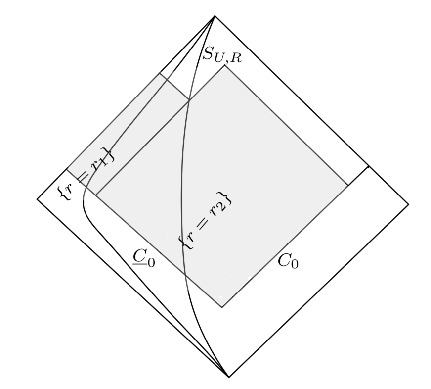
Figure 1: Penrose diagram of Reissner-Nordström spacetime. For every $S_{U,R}$, the gray area describes the area where the estimates are obtained.

Since the estimates in the proof of decay do not depend on $U$ and $R$, in the above construction $U$ and $R$ can be taken to be arbitrarily large. As $U$ and $R$ vary to arbitrarily large values, the regions constructed as above cover the whole exterior region in the future of $C_{0}\cup\underline{C}_{0}$, and therefore the above proves the validity of the estimates in the whole exterior region. See Section 12.4.7 for more details about the conclusion of the proof.

We also point out here that the proof of boundedness of the solution using the initial-data normalization could have been avoided in the final proof of decay by performing a bootstrap argument. By choosing the maximal $U$ and $R$ for which the solution was assumed to be bounded, and then adding the far-away normalization, one can prove that the solution was bounded (and actually decays) in the full exterior. On the other hand, the proof of boundedness here presented has the advantage of making clear the necessity of the far-away normalization in order to obtain a decay consistent with non-linear applications, and also helps to draw a clear analogy with [9].

1.6 The identification of the final parameters $M$, $Q$, and $a$

The decay described above corresponds to the gravitational and electromagnetic radiation emitted by the perturbation of the Reissner-Nordström black hole as it settles down to a member of the Kerr-Newman family with final parameters $M$, $Q$, and $a$.

The projection to the $\ell=0$ spherical harmonics of the perturbation contains the spherically symmetric solutions, which correspond to other Reissner-Nordström spacetimes with modified mass $M$ and charge $Q$. The projection to the $\ell=1$ spherical harmonics contains instead the axially symmetric solutions, which correspond to a slowly rotating Kerr-Newman spacetime with small angular momentum $a$. These special solutions are called linearized Kerr-Newman solutions, as in Definition 6.1.

This change in parameters can be identified in linear theory from the projection to the $\ell=0$ and $\ell=1$ spherical harmonics at the initial data, similarly to [9].

1.7 Outline

We outline here the structure of the paper.

In Section 2, we derive the general form of the Einstein-Maxwell equations written with respect to a local null frame. In Section 3, we introduce our choice of gauge, the Bondi gauge, to be used in the linear perturbations of Reissner-Nordström spacetime.

In Section 4, we describe the Reissner-Nordström spacetime, which is the background solution around which we perform the gravitational and electromagnetic perturbations. In Section 5, we derive the linearized Einstein-Maxwell equations around the Reissner-Nordström solution. We denote a linear gravitational and electromagnetic perturbation of Reissner-Nordström a set of components which is a solution to those equations. In Section 6, we present special solutions to the linearized Einstein-Maxwell equations around the Reissner-Nordström: pure gauge solutions and linearized Kerr-Newman solutions.

In Section 7, we state the precise version of our main Theorem. In Section 8, we summarize the results on the boundedness and decay for the solutions to the Teukolsky system as proved in [15] and [16].

In Section 9, we present the characteristic initial problem and the well-posedness of the linearized Einstein-Maxwell equations. In Section 10 we describe the two gauge normalization which we will use and the final Kerr-Newman parameters.

In Section 11, we prove boundedness of the solution using the initial data normalization and in Section 12 we finally prove decay for all the gauge-dependent components of the solution, therefore obtaining the proof of quantitative linear stability.

In the Appendix A, we present explicit computations.

Acknowledgements The author would like to thank Sergiu Klainerman and Mu-Tao Wang for their guidance and support. The author is also grateful to Jérémie Szeftel, Pei-Ken Hung and Federico Pasqualotto for helpful discussions. The author is grateful to the anonymous referee for several helpful suggestions.

2 The Einstein-Maxwell equations in null frames

In this section, we derive the general form of the Einstein-Maxwell equations (2) and (3) written with respect to a local null frame attached to a general foliation of a Lorentzian manifold. In this section, we do not restrict to a specific form of the metric and derive the main equations in their full generality. It is these equations we shall linearize in Section 5 to obtain the equations for a linear gravitational and electromagnetic perturbation of a spacetime.

We begin in Section 2.1 with preliminaries, recalling the notion of local null frame and tensor algebra. In Section 2.2, we define Ricci coefficients, curvature and electromagnetic components of a solution to the Einstein-Maxwell equations. Finally, we present the Einstein-Maxwell equations in Section 2.3.

2.1 Preliminaries

Let $({\mathcal{M}},{\bf g})$ be a $3+1$-dimensional Lorentzian manifold, and let ${\bf D}$ be the covariant derivative associated to ${\bf g}$.

Suppose that the the Lorentzian manifold $({\mathcal{M}},{\bf g})$ can be foliated by spacelike $2$-surfaces $(S,\not{g})$, where $\not{g}$ is the pullback of the metric ${\bf g}$ to $S$. To each point of ${\mathcal{M}}$, we can associate a null frame $\mathscr{N}=\left\{e_{A},e_{3},e_{4}\right\}$, with $\{e_{A}\}_{A=1,2}$ being tangent vectors to $(S,\not{g})$, such that the following relations hold:

$$\begin{split}{\bf g}\left(e_{3},e_{3}\right)&=0,\qquad{\bf g}\left(e_{4},e_{4}\right)=0,\qquad{\bf g}\left(e_{3},e_{4}\right)=-2\\ {\bf g}\left(e_{3},e_{A}\right)&=0\ \ \ ,\ \ \ {\bf g}\left(e_{4},e_{A}\right)=0\ \ \ ,\ \ \ {\bf g}\left(e_{A},e_{B}\right)=\not{g}_{AB}\,.\end{split}$$ (9)

The surfaces $S$ will be identified in Chapter 3 as intersections of two specified hypersurfaces. Similarly, after a choice of gauge, the frame $\mathscr{N}$ can be identified explicitly in terms of coordinates. See Section 3.1 for the identification of the null frame in the Bondi gauge.

In the following section, we will express the Ricci coefficients, curvature and electromagnetic components with respect to a null frame $\mathscr{N}$ associated to a foliation of surfaces $S$. The objects we shall define are therefore $S$-tangent tensors. We recall here the standard notations for operations on $S$-tangent tensors. (See [8] and [9])

We recall the definition of the projected covariant derivatives and the angular operator on $S$-tensors. We denote $\nabla\mkern-13.0mu/\,_{3}=\nabla\mkern-13.0mu/\,_{e_{3}}$ and $\nabla\mkern-13.0mu/\,_{4}=\nabla\mkern-13.0mu/\,_{e_{4}}$ the projection to $S$ of the spacetime covariant derivatives ${\bf D}_{e_{3}}$ and ${\bf D}_{e_{4}}$ respectively. We denote by $\underline{D}\chi$ and $D\chi$ the projected Lie derivative with respect to $e_{3}$ and $e_{4}$. The relations between them are the following:

$$\begin{split}Df&=\nabla\mkern-13.0mu/\,_{4}(f),\\ D\xi_{A}&=\nabla\mkern-13.0mu/\,_{4}\xi_{A}+\chi_{AB}\xi^{B},\\ D\theta_{AB}&=\nabla\mkern-13.0mu/\,_{4}\theta_{AB}+\chi_{AC}{\theta^{C}}_{B}+\chi_{BC}{\theta_{A}}^{C}\end{split}$$ (10)

and similarly for $e_{3}$ replacing $\chi$ by $\underline{\chi}$, where $\chi$ and $\underline{\chi}$ are defined in (21).

We recall the following angular operators on $S$-tensors.

Let $\xi$ be an arbitrary one-form and $\theta$ an arbitrary symmetric traceless $2$-tensor on $S$.

• $\nabla\mkern-13.0mu/\,$ denotes the covariant derivative associated to the metric $\not{g}$ on $S$.

• $\,{\mathcal{D}}\mkern-8.0mu/_{1}$ takes $\xi$ into the pair of functions $(\mbox{div}\mkern-19.0mu/\,\,\,\,\xi,\mbox{curl}\mkern-19.0mu/\,\,\,\,\xi)$, where

  $$\mbox{div}\mkern-19.0mu/\,\,\,\,\xi=\not{g}^{AB}\nabla\mkern-13.0mu/\,_{A}\xi_{B},\qquad\mbox{curl}\mkern-19.0mu/\,\,\,\,\xi=\epsilon^{AB}\nabla\mkern-13.0mu/\,_{A}\xi_{B}$$

• $\,{\mathcal{D}}{\,{}^{\star}\mkern-2.0mu}\mkern-16.0mu/_{1}$ is the formal $L^{2}$-adjoint of $\,{\mathcal{D}}\mkern-8.0mu/_{1}$, and takes any pair of functions $(\rho,\sigma)$ into the one-form $-\nabla\mkern-13.0mu/\,_{A}\rho+\epsilon_{AB}\nabla\mkern-13.0mu/\,^{B}\sigma$.

• $\,{\mathcal{D}}\mkern-8.0mu/_{2}$ takes $\theta$ into the one-form $\,{\mathcal{D}}\mkern-8.0mu/_{2}\theta=(\mbox{div}\mkern-19.0mu/\,\,\,\,\theta)_{C}=\not{g}^{AB}\nabla\mkern-13.0mu/\,_{A}\theta_{BC}$.

• $\,{\mathcal{D}}{\,{}^{\star}\mkern-2.0mu}\mkern-16.0mu/_{2}$ is the formal $L^{2}$-adjoint of $\,{\mathcal{D}}\mkern-8.0mu/_{2}$, and takes $\xi$ into the symmetric traceless two tensor

  $$(\,{\mathcal{D}}{\,{}^{\star}\mkern-2.0mu}\mkern-16.0mu/_{2}\xi)_{AB}=-\frac{1}{2}\left(\nabla\mkern-13.0mu/\,_{B}\xi_{A}+\nabla\mkern-13.0mu/\,_{A}\xi_{B}-(\mbox{div}\mkern-19.0mu/\,\,\,\,\xi)\not{g}_{AB}\right)$$

We can easily check that $\,{\mathcal{D}}{\,{}^{\star}\mkern-2.0mu}\mkern-16.0mu/_{k}$ is the formal adjoint of $\,{\mathcal{D}}\mkern-8.0mu/_{k}$, i.e.

$$\int_{S}(\,{\mathcal{D}}\mkern-8.0mu/_{k}f)g=\int_{S}f(\,{\mathcal{D}}{\,{}^{\star}\mkern-2.0mu}\mkern-16.0mu/_{k}g)$$

We recall the following $L^{2}$ elliptic estimates. (see [8] or [25]).

Proposition 2.1.1.

Let $(S,\not{g})$ be a compact surface with Gauss curvature $K$.

1. The following identity holds for a pair of functions $(\rho,\sigma)$ on $S$:

   $$\int_{S}\left(|\nabla\mkern-13.0mu/\,\rho|^{2}+|\nabla\mkern-13.0mu/\,\sigma|^{2}\right) = \int_{S}|\,{\mathcal{D}}{\,{}^{\star}\mkern-2.0mu}\mkern-16.0mu/_{1}(\rho,\sigma)|^{2}$$ (11)

2. The following identity holds for $1$-forms $\xi$ on $S$:

   $$\int_{S}\left(|\nabla\mkern-13.0mu/\,\xi|^{2}+K|\xi|^{2}\right) = \int_{S}\left(|\mbox{div}\mkern-19.0mu/\,\,\,\,\xi|^{2}+|\mbox{curl}\mkern-19.0mu/\,\,\,\,\xi|^{2}\right)=\int_{S}|\,{\mathcal{D}}\mkern-8.0mu/_{1}\xi|^{2}$$ (12)

   $$\int_{S}\left(|\nabla\mkern-13.0mu/\,\xi|^{2}-K|\xi|^{2}\right) = 2\int_{S}|\,{\mathcal{D}}{\,{}^{\star}\mkern-2.0mu}\mkern-16.0mu/_{2}\xi|^{2}$$ (13)

3. The following identity holds for symmetric traceless $2$-tensors $\theta$ on $S$:

   $$\int_{S}\left(|\nabla\mkern-13.0mu/\,\theta|^{2}+2K|\theta|^{2}\right) = 2\int_{S}|\mbox{div}\mkern-19.0mu/\,\,\,\,\theta|^{2}=2\int_{S}|\,{\mathcal{D}}\mkern-8.0mu/_{2}\theta|^{2}$$ (14)

4. Suppose that the Gauss curvature is bounded away from zero. Then there exists a constant $C>0$ such that the following estimate holds for all vectors $\xi$ on $S$ orthogonal to the kernel of $\,{\mathcal{D}}{\,{}^{\star}\mkern-2.0mu}\mkern-16.0mu/_{2}$:

   $$\int_{S}\frac{1}{r^{2}}|\xi|^{2}\leq C\int_{S}|\,{\mathcal{D}}{\,{}^{\star}\mkern-2.0mu}\mkern-16.0mu/_{2}\xi|^{2}$$ (15)

   where $r$ is the radial area function, i.e. $|S|=4\pi r^{2}$.

Given $f$ a $S$-tensor, we define $\mbox{$\bigtriangleup\mkern-13.0mu/\,$}f=\not{g}^{AB}\nabla\mkern-13.0mu/\,_{A}\nabla\mkern-13.0mu/\,_{B}f$. We recall the relations between the angular operators and the laplacian $\bigtriangleup\mkern-13.0mu/\,$ on $S$:

$$\begin{split}\,{\mathcal{D}}\mkern-8.0mu/_{1}\,{\mathcal{D}}{\,{}^{\star}\mkern-2.0mu}\mkern-16.0mu/_{1}&=-\mbox{$\bigtriangleup\mkern-13.0mu/\,$}_{0},\qquad\,{\mathcal{D}}{\,{}^{\star}\mkern-2.0mu}\mkern-16.0mu/_{1}\,{\mathcal{D}}\mkern-8.0mu/_{1}=-\mbox{$\bigtriangleup\mkern-13.0mu/\,$}_{1}+K,\\ \,{\mathcal{D}}\mkern-8.0mu/_{2}\,{\mathcal{D}}{\,{}^{\star}\mkern-2.0mu}\mkern-16.0mu/_{2}&=-\frac{1}{2}\mbox{$\bigtriangleup\mkern-13.0mu/\,$}_{1}-\frac{1}{2}K,\qquad\,{\mathcal{D}}{\,{}^{\star}\mkern-2.0mu}\mkern-16.0mu/_{2}\,{\mathcal{D}}\mkern-8.0mu/_{2}=-\frac{1}{2}\mbox{$\bigtriangleup\mkern-13.0mu/\,$}_{2}+K\end{split}$$ (16)

where $\mbox{$\bigtriangleup\mkern-13.0mu/\,$}_{0}$, $\mbox{$\bigtriangleup\mkern-13.0mu/\,$}_{1}$ and $\mbox{$\bigtriangleup\mkern-13.0mu/\,$}_{2}$ are the Laplacian on scalars, on $1$-forms and on symmetric traceless $2$-tensors respectively, and $K$ is the Gauss curvature of the surface $S$.

Let $f$ be a scalar on ${\mathcal{M}}$. We define its $S$-average, and denote it by $\overline{f}$ as

$$\overline{f}: = \frac{1}{|S|}\int_{S}f$$ (17)

where $|S|$ denotes the volume of $(S,\not{g})$. We define the derived scalar function $\check{f}$ as

$$\check{f}:=f-\overline{f}.$$ (18)

It follows from the definition that, for two functions $f$ and $g$,

$$\overline{fg} = \overline{f}\overline{g}+\overline{\check{f}\check{g}},$$ (19)

$$\check{fg} = fg-\overline{fg}=\check{f}\overline{g}+\overline{f}\check{g}+(\check{f}\check{g}-\overline{\check{f}\check{g}})$$ (20)

2.2 Ricci coefficients, curvature and electromagnetic components

We now define the Ricci coefficients, curvature and electromagnetic components associated to the metric ${\bf g}$ with respect to the null frame $\mathscr{N}=\left\{e_{A},e_{3},e_{4}\right\}$, where the indices $A,B$ take values $1,2$. We follow the standard notations in [8].

2.2.1 Ricci coefficients

We define the Ricci coefficients associated to the metric ${\bf g}$ with respect to the null frame $\mathscr{N}$:

$$\begin{split}\chi_{AB}:&={\bf g}({\bf D}_{A}e_{4},e_{B}),\qquad\underline{\chi}_{AB}:={\bf g}({\bf D}_{A}e_{3},e_{B})\\ \eta_{A}:&=\frac{1}{2}{\bf g}({\bf D}_{3}e_{4},e_{A}),\qquad\underline{\eta}_{A}:=\frac{1}{2}{\bf g}({\bf D}_{4}e_{3},e_{A}),\\ \xi_{A}:&=\frac{1}{2}{\bf g}({\bf D}_{4}e_{4},e_{A}),\qquad\underline{\xi}_{A}:=\frac{1}{2}{\bf g}({\bf D}_{3}e_{3},e_{A})\\ \omega:&=\frac{1}{4}{\bf g}({\bf D}_{4}e_{4},e_{3}),\qquad{\underline{\omega}}:=\frac{1}{4}{\bf g}({\bf D}_{3}e_{3},e_{4})\\ \zeta_{A}:&=\frac{1}{2}{\bf g}({\bf D}_{A}e_{4},e_{3}),\qquad\end{split}$$ (21)

We decompose the $2$-tensor $\chi_{AB}$ into its tracefree part $\widehat{\chi}_{AB}$, a symmetric traceless 2-tensor on $S$, and its trace. We define

$$\kappa:=\mbox{tr}\chi\qquad\underline{\kappa}:=\mbox{tr}\underline{\chi}$$ (22)

In particular we write $\chi_{AB}=\frac{1}{2}\kappa\ \not{g}_{AB}+\widehat{\chi}_{AB}$, with $\not{g}^{AB}\widehat{\chi}_{AB}=0$ and $\kappa=\not{g}^{AB}\chi_{AB}$. Similarly for $\underline{\chi}_{AB}$.

It follows from (21) that we have the following relations for the covariant derivatives of the null frame:

$$\begin{split}{\bf D}_{4}e_{4}&=-2\omega e_{4}+2\xi^{A}e_{A},\qquad{\bf D}_{3}e_{3}=-2{\underline{\omega}}e_{3}+2\underline{\xi}^{A}e_{A},\\ {\bf D}_{4}e_{3}&=2\omega e_{3}+2\underline{\eta}^{A}e_{A},\qquad{\bf D}_{3}e_{4}=2{\underline{\omega}}e_{4}+2\eta^{A}e_{A},\\ {\bf D}_{4}e_{A}&=\nabla\mkern-13.0mu/\,_{4}e_{A}+\underline{\eta}_{A}e_{4}+\xi_{A}e_{3},\qquad{\bf D}_{3}e_{A}=\nabla\mkern-13.0mu/\,_{3}e_{A}+\eta_{A}e_{3}+\underline{\xi}_{A}e_{4},\\ {\bf D}_{A}e_{4}&=-\zeta_{A}e_{4}+\chi_{AB}e^{B},\qquad{\bf D}_{A}e_{3}=\zeta_{A}e_{3}+\underline{\chi}_{AB}e^{B},\\ {\bf D}_{A}e_{B}&=\nabla\mkern-13.0mu/\,_{A}e_{B}+\frac{1}{2}\underline{\chi}_{AB}e_{4}+\frac{1}{2}\chi_{AB}e_{3}.\end{split}$$ (23)

The following relations for the commutators of the null frame also follow from (21):

$$\begin{split}\big{[}e_{3},e_{A}\big{]}&=\nabla\mkern-13.0mu/\,_{3}e_{A}+(\eta_{A}-\zeta_{A})e_{3}+\underline{\xi}_{A}e_{4}-\underline{\chi}_{AB}e^{B},\\ \big{[}e_{4},e_{A}\big{]}&=\nabla\mkern-13.0mu/\,_{4}e_{A}+(\underline{\eta}_{A}+\zeta_{A})e_{4}+\xi_{A}e_{3}-\chi_{AB}e^{B},\\ \big{[}e_{3},e_{4}\big{]}&=-2\omega e_{3}+2{\underline{\omega}}e_{4}+2(\eta^{A}-\underline{\eta}^{A})e_{A}\end{split}$$ (24)

2.2.2 Curvature components

Let ${\bf W}$ denote the Weyl curvature of ${\bf g}$ and let ${\,{}^{\star}\mkern-2.0mu}{\bf W}$ denote the Hodge dual on $({\mathcal{M}},{\bf g})$ of ${\bf W}$, defined by ${\,{}^{\star}\mkern-2.0mu}{\bf W}_{\alpha\beta\gamma\delta}=\frac{1}{2}\epsilon_{\alpha\beta\mu\nu}{{\bf W}^{\mu\nu}}_{\gamma\delta}$.

We define the null curvature components:

$$\begin{split}\alpha_{AB}:&={\bf W}(e_{A},e_{4},e_{B},e_{4}),\qquad\underline{\alpha}_{AB}:={\bf W}(e_{A},e_{3},e_{B},e_{3})\\ \beta_{A}:&=\frac{1}{2}{\bf W}(e_{A},e_{4},e_{3},e_{4}),\qquad\underline{\beta}_{A}:=\frac{1}{2}{\bf W}(e_{A},e_{3},e_{3},e_{4})\\ \rho:&=\frac{1}{4}{\bf W}(e_{3},e_{4},e_{3},e_{4})\qquad\sigma:=\frac{1}{4}{\,{}^{\star}\mkern-2.0mu}{\bf W}(e_{3},e_{4},e_{3},e_{4})\end{split}$$ (25)

The remaining components of the Weyl tensor are given by

$${\bf W}_{AB34}=2\sigma\epsilon_{AB},\qquad{\bf W}_{ABC3}=\epsilon_{AB}{\,{}^{\star}\mkern-2.0mu}\underline{\beta}_{C},\qquad{\bf W}_{ABC4}=-\epsilon_{AB}{\,{}^{\star}\mkern-2.0mu}\beta_{C},$$

$${\bf W}_{A3B4}=-\rho\not{g}_{AB}+\sigma\epsilon_{AB},\qquad{\bf W}_{ABCD}=-\epsilon_{AB}\epsilon_{CD}\rho$$

Note that in this formula the star is the Hodge dual on spheres. Observe that when interchanging $e_{3}$ with $e_{4}$, the one form $\beta$ becomes $-\underline{\beta}$, the scalar $\sigma$ changes sign, while $\rho$ remains unchanged.

2.2.3 Electromagnetic components

Let ${\bf F}$ be a $2$-form in $({\mathcal{M}},{\bf g})$, and let ${\,{}^{\star}\mkern-2.0mu}{\bf F}$ denote the Hodge dual on $({\mathcal{M}},{\bf g})$ of ${\bf F}$, defined by ${\,{}^{\star}\mkern-2.0mu}{\bf F}_{\alpha\beta}=\frac{1}{2}\epsilon_{\mu\nu\alpha\beta}{\bf F}^{\mu\nu}$.

We define the null electromagnetic components:

$$\begin{split}\,{}^{(F)}\beta_{A}:&={\bf F}(e_{A},e_{4}),\qquad\,^{(F)}\underline{\beta}_{A}:={\bf F}(e_{A},e_{3})\\ \,{}^{(F)}\rho:=&\frac{1}{2}{\bf F}(e_{3},e_{4}),\qquad\,^{(F)}\sigma:=\frac{1}{2}{\,{}^{\star}\mkern-2.0mu}{\bf F}(e_{3},e_{4})\end{split}$$ (26)

The only remaining component of ${\bf F}$ is given by ${\bf F}_{AB}=-\epsilon_{AB}\,^{(F)}\sigma$.

Observe that when interchanging $e_{3}$ with $e_{4}$, the scalar $\,{}^{(F)}\rho$ changes sign, while $\,{}^{(F)}\sigma$ remains unchanged.

2.3 The Einstein-Maxwell equations

If $({\mathcal{M}},{\bf g})$ satisfies the Einstein-Maxwell equations

$${\bf R}_{\mu\nu} = 2{\bf F}_{\mu\lambda}{{\bf F}_{\nu}}^{\lambda}-\frac{1}{2}{\bf g}_{\mu\nu}{\bf F}^{\alpha\beta}{\bf F}_{\alpha\beta},$$ (27)

$${\bf D}_{[\alpha}{\bf F}_{\beta\gamma]} = 0,\qquad{\bf D}^{\alpha}{\bf F}_{\alpha\beta}=0.$$ (28)

the Ricci coefficients, curvature and electromagnetic components defined in (21), (25) and (26) satisfy a system of equations, which is presented in this section.

2.3.1 Decomposition of Ricci and Riemann curvature

The Ricci curvature of $({\mathcal{M}},{\bf g})$ can be expressed in terms of the electromagnetic null decomposition according to Einstein equation (27). We compute the following components of the Ricci tensor.

$${\bf R}_{A3} = 2{\bf F}_{A\lambda}{{\bf F}_{3}}^{\lambda}=2\not{g}^{BC}{\bf F}_{AB}{\bf F}_{3C}-{\bf F}_{A3}{\bf F}_{34}=2\,^{(F)}\sigma{\epsilon_{A}}^{C}\,{}^{(F)}\underline{\beta}_{C}-2\,^{(F)}\rho\,^{(F)}\underline{\beta}_{A},$$

$${\bf R}_{A4} = 2\,^{(F)}\sigma{\epsilon_{A}}^{C}\,{}^{(F)}\beta_{C}+2\,^{(F)}\rho\,^{(F)}\beta_{A},$$

$${\bf R}_{33} = 2{\bf g}^{\lambda\mu}{\bf F}_{3\lambda}{\bf F}_{3\mu}=2\not{g}^{AB}{\bf F}_{3A}{\bf F}_{3B}=2\,^{(F)}\underline{\beta}\cdot\,^{(F)}\underline{\beta},$$

$${\bf R}_{34} = {\bf g}^{34}({\bf F}_{34})^{2}+\not{g}^{AB}\not{g}^{CD}{\bf F}_{AC}{\bf F}_{DB}=2\,^{(F)}\rho^{2}+2\,^{(F)}\sigma^{2}$$

$${\bf R}_{44} = 2\,^{(F)}\beta\cdot\,^{(F)}\beta,$$

$${\bf R}_{AB} = 2{\bf F}_{A\lambda}{{\bf F}_{B}}^{\lambda}-\not{g}_{AB}{{\bf F}^{D}}_{\lambda}{{\bf F}^{\lambda}}_{D}+\frac{1}{2}\not{g}_{AB}{\bf R}_{34}=-2(\,^{(F)}\beta\widehat{\otimes}\,^{(F)}\underline{\beta})_{AB}+(\,^{(F)}\rho^{2}+\,^{(F)}\sigma^{2})\not{g}_{AB}$$

We denote $\widehat{\otimes}$ the symmetric traceless tensor product. Observe that as a consequence of (27), the scalar curvature of the metric ${\bf g}$ is zero, therefore we have $\not{{\bf g}}^{AC}{\bf R}_{AC}={\bf R}_{34}$.

Using the decomposition of the Riemann curvature in Weyl curvature and Ricci tensor:

$${\bf R}_{\alpha\beta\gamma\delta}={\bf W}_{\alpha\beta\gamma\delta}+\frac{1}{2}({\bf g}_{\beta\delta}{\bf R}_{\alpha\gamma}+{\bf g}_{\alpha\gamma}{\bf R}_{\beta\delta}-{\bf g}_{\beta\gamma}{\bf R}_{\alpha\delta}-{\bf g}_{\alpha\delta}{\bf R}_{\beta\gamma}),$$ (29)

we can express the full Riemann tensor of $({\mathcal{M}},{\bf g})$ in terms of the above decompositions. We compute the following components of the Riemann tensor.

$${\bf R}_{A33B} = {\bf W}_{A33B}-\frac{1}{2}\not{g}_{AB}{\bf R}_{33}=-\underline{\alpha}_{AB}-(\,^{(F)}\underline{\beta}\cdot\,^{(F)}\underline{\beta})\not{g}_{AB},$$

$${\bf R}_{A34B} = {\bf W}_{A34B}+{\bf R}_{AB}-\frac{1}{2}\not{g}_{AB}{\bf R}_{34}=\rho\ \not{g}_{AB}-\sigma\epsilon_{AB}-(\,^{(F)}\beta\widehat{\otimes}\,^{(F)}\underline{\beta})_{AB},$$

$${\bf R}_{A334} = {\bf W}_{A334}-{\bf R}_{A3}=2\underline{\beta}_{A}-2\,^{(F)}\sigma{\epsilon_{A}}^{C}\,{}^{(F)}\underline{\beta}_{C}+2\,^{(F)}\rho\,^{(F)}\underline{\beta}_{A},$$

$${\bf R}_{3434} = {\bf W}_{3434}+2{\bf R}_{34}=4\rho+4\,^{(F)}\rho^{2}+4\,^{(F)}\sigma^{2},$$

$${\bf R}_{A3CB} = {\bf W}_{A3CB}+\frac{1}{2}(\not{g}_{AC}{\bf R}_{3B}-\not{g}_{AB}{\bf R}_{3C})$$

$$= \epsilon_{CB}{\,{}^{\star}\mkern-2.0mu}\underline{\beta}_{A}+\not{g}_{AC}(\,^{(F)}\sigma{\epsilon_{B}}^{C}\,{}^{(F)}\underline{\beta}_{C}-\,^{(F)}\rho\,^{(F)}\underline{\beta}_{B})-\not{g}_{AB}(\,^{(F)}\sigma{\epsilon_{C}}^{D}\,{}^{(F)}\underline{\beta}_{D}-\,^{(F)}\rho\,^{(F)}\underline{\beta}_{C}),$$

$${\bf R}_{ABCD} = {\bf W}_{ABCD}+\frac{1}{2}({\bf g}_{BD}{\bf R}_{AC}+{\bf g}_{AC}{\bf R}_{BD}-{\bf g}_{BC}{\bf R}_{AD}-{\bf g}_{AD}{\bf R}_{BC})$$

We will use the above decompositions of Ricci and Riemann curvature in the derivation of the equations in Sections 2.3.2-2.3.4.

2.3.2 The null structure equations

The first equation for $\chi$ and $\underline{\chi}$ is given by

$$\nabla\mkern-13.0mu/\,_{3}\underline{\chi}_{AB}+\underline{\chi}_{A}^{C}\underline{\chi}_{CB}+2{\underline{\omega}}\underline{\chi}_{AB} = 2\nabla\mkern-13.0mu/\,_{B}\underline{\xi}_{A}+2\eta_{B}\underline{\xi}_{A}+2\underline{\eta}_{A}\underline{\xi}_{B}-4\zeta_{B}\underline{\xi}_{A}+{\bf R}_{A33B}$$

$$\nabla\mkern-13.0mu/\,_{4}\chi_{AB}+\chi_{A}^{C}\chi_{CB}+2\omega\chi_{AB} = 2\nabla\mkern-13.0mu/\,_{B}\xi_{A}+2\eta_{B}\xi_{A}+2\eta_{A}\xi_{B}+4\zeta_{B}\xi_{A}+{\bf R}_{A44B}$$

We separate them in the symmetric traceless part, the trace part and the antisymmetric part. We obtain respectively:

$$\begin{split}\nabla\mkern-13.0mu/\,_{3}\widehat{\underline{\chi}}+\underline{\kappa}\ \widehat{\underline{\chi}}+2{\underline{\omega}}\widehat{\underline{\chi}}&=&-2\,{\mathcal{D}}{\,{}^{\star}\mkern-2.0mu}\mkern-16.0mu/_{2}\underline{\xi}-\underline{\alpha}+2(\eta+\underline{\eta}-2\zeta)\widehat{\otimes}\underline{\xi}\\ \nabla\mkern-13.0mu/\,_{4}\widehat{\chi}+\kappa\ \widehat{\chi}+2\omega\widehat{\chi}&=&-2\,{\mathcal{D}}{\,{}^{\star}\mkern-2.0mu}\mkern-16.0mu/_{2}\xi-\alpha+2(\eta+\underline{\eta}+2\zeta)\widehat{\otimes}\xi\end{split}$$ (30)

$$\begin{split}\nabla\mkern-13.0mu/\,_{3}\underline{\kappa}+\frac{1}{2}\underline{\kappa}^{2}+2{\underline{\omega}}\underline{\kappa}=2\mbox{div}\mkern-19.0mu/\,\,\,\,\underline{\xi}-\widehat{\underline{\chi}}\cdot\widehat{\underline{\chi}}+2(\eta+\underline{\eta}-2\zeta)\cdot\underline{\xi}-2\,^{(F)}\underline{\beta}\cdot\,^{(F)}\underline{\beta}\\ \nabla\mkern-13.0mu/\,_{4}\kappa+\frac{1}{2}\kappa^{2}+2\omega\kappa=2\mbox{div}\mkern-19.0mu/\,\,\,\,\xi-\widehat{\chi}\cdot\widehat{\chi}+2(\eta+\underline{\eta}+2\zeta)\cdot\xi-2\,^{(F)}\beta\cdot\,^{(F)}\beta\end{split}$$ (31)

$$\begin{split}\mbox{curl}\mkern-19.0mu/\,\,\,\,\underline{\xi}&=&\underline{\xi}\wedge(\eta+\underline{\eta}-2\zeta)\\ \mbox{curl}\mkern-19.0mu/\,\,\,\,\xi&=&\xi\wedge(\eta+\underline{\eta}+2\zeta)\end{split}$$ (32)

where $\xi\wedge\eta=\epsilon_{AB}\xi^{A}\eta^{B}$.

The second equation for $\chi$ and $\underline{\chi}$ is given by

$$\nabla\mkern-13.0mu/\,_{4}\underline{\chi}_{AB} = 2\nabla\mkern-13.0mu/\,_{B}\underline{\eta}_{A}+2\omega\underline{\chi}_{AB}-\chi_{B}^{C}\underline{\chi}_{AC}+2(\xi_{B}\underline{\xi}_{A}+\underline{\eta}_{B}\underline{\eta}_{A})+{\bf R}_{A34B}$$

$$\nabla\mkern-13.0mu/\,_{3}\chi_{AB} = 2\nabla\mkern-13.0mu/\,_{B}\eta_{A}+2{\underline{\omega}}\chi_{AB}-\underline{\chi}_{B}^{C}\chi_{AC}+2(\underline{\xi}_{B}\xi_{A}+\eta_{B}\eta_{A})+{\bf R}_{A43B}$$

We separate them in the symmetric traceless part, the trace part and the antisymmetric part. We obtain respectively

$$\begin{split}\nabla\mkern-13.0mu/\,_{3}\widehat{\chi}+\frac{1}{2}\underline{\kappa}\,\widehat{\chi}-2{\underline{\omega}}\widehat{\chi}&=&-2\not{\mathcal{D}}_{2}^{\star}\eta-\frac{1}{2}\kappa\widehat{\underline{\chi}}+2\eta\widehat{\otimes}\eta+2\underline{\xi}\widehat{\otimes}\xi-2\,^{(F)}\beta\widehat{\otimes}\,^{(F)}\underline{\beta}\\ \nabla\mkern-13.0mu/\,_{4}\widehat{\underline{\chi}}+\frac{1}{2}\kappa\,\widehat{\underline{\chi}}-2\omega\widehat{\underline{\chi}}&=&-2\not{\mathcal{D}}_{2}^{\star}\underline{\eta}-\frac{1}{2}\underline{\kappa}\widehat{\chi}+2\underline{\eta}\widehat{\otimes}\underline{\eta}+2\underline{\xi}\widehat{\otimes}\xi-2\,^{(F)}\beta\widehat{\otimes}\,^{(F)}\underline{\beta}\end{split}$$ (33)

$$\begin{split}\nabla\mkern-13.0mu/\,_{3}\kappa+\frac{1}{2}\kappa\,\underline{\kappa}-2{\underline{\omega}}\,\kappa&=&2\mbox{div}\mkern-19.0mu/\,\,\,\,\eta-\widehat{\chi}\cdot\widehat{\underline{\chi}}+2\xi\cdot\underline{\xi}+2\eta\cdot\eta+2\rho\\ \nabla\mkern-13.0mu/\,_{4}\underline{\kappa}+\frac{1}{2}\kappa\,\underline{\kappa}-2\omega\,\underline{\kappa}&=&2\mbox{div}\mkern-19.0mu/\,\,\,\,\underline{\eta}-\widehat{\chi}\cdot\widehat{\underline{\chi}}+2\xi\cdot\underline{\xi}+2\underline{\eta}\cdot\underline{\eta}+2\rho\end{split}$$ (34)

$$\begin{split}\not{\mbox{curl }}\eta&=&-\frac{1}{2}\chi\wedge\underline{\chi}+\sigma,\\ \not{\mbox{curl }}\underline{\eta}&=&\frac{1}{2}\chi\wedge\underline{\chi}-\sigma\end{split}$$ (35)

The equations for $\zeta$ are given by

$$\nabla\mkern-13.0mu/\,_{3}\zeta = -2\nabla\mkern-13.0mu/\,{\underline{\omega}}-\underline{\chi}\cdot(\zeta+\eta)+2{\underline{\omega}}(\zeta-\eta)+\chi\cdot\underline{\xi}+2\omega\underline{\xi}-\frac{1}{2}{\bf R}_{A334},$$

$$-\nabla\mkern-13.0mu/\,_{4}\zeta = -2\nabla\mkern-13.0mu/\,\omega-\chi\cdot(-\zeta+\underline{\eta})+2\omega(-\zeta-\underline{\eta})+\underline{\chi}\cdot\xi+2{\underline{\omega}}\xi-\frac{1}{2}{\bf R}_{A443}$$

and therefore reducing to

$$\begin{split}\nabla\mkern-13.0mu/\,_{3}\zeta&=&-2\nabla\mkern-13.0mu/\,{\underline{\omega}}-\underline{\chi}\cdot(\zeta+\eta)+2{\underline{\omega}}(\zeta-\eta)+\chi\cdot\underline{\xi}+2\omega\underline{\xi}-\underline{\beta}+\,^{(F)}\sigma{\epsilon_{A}}^{C}\,{}^{(F)}\underline{\beta}_{C}-\,^{(F)}\rho\,^{(F)}\underline{\beta},\\ \nabla\mkern-13.0mu/\,_{4}\zeta&=&2\nabla\mkern-13.0mu/\,\omega+\chi\cdot(-\zeta+\underline{\eta})+2\omega(\zeta+\underline{\eta})-\underline{\chi}\cdot\xi-2{\underline{\omega}}\xi-\beta-\,^{(F)}\sigma\epsilon\cdot\,^{(F)}\beta-\,^{(F)}\rho\,^{(F)}\beta\end{split}$$ (36)

The equations for $\xi$ and $\underline{\xi}$ are given by

$$\nabla\mkern-13.0mu/\,_{4}\underline{\xi}-\nabla\mkern-13.0mu/\,_{3}\underline{\eta} = 4\omega\underline{\xi}-\underline{\chi}\cdot(\eta-\underline{\eta})-\frac{1}{2}{\bf R}_{A334},$$

$$\nabla\mkern-13.0mu/\,_{3}\xi-\nabla\mkern-13.0mu/\,_{4}\eta = 4{\underline{\omega}}\xi+\chi\cdot(\eta-\underline{\eta})-\frac{1}{2}{\bf R}_{A443}$$

and therefore reducing to

$$\begin{split}\nabla\mkern-13.0mu/\,_{4}\underline{\xi}-\nabla\mkern-13.0mu/\,_{3}\underline{\eta}&=&-\underline{\chi}\cdot(\eta-\underline{\eta})+4\omega\underline{\xi}-\underline{\beta}+\,^{(F)}\sigma\epsilon\cdot\,^{(F)}\underline{\beta}-\,^{(F)}\rho\,^{(F)}\underline{\beta},\\ \nabla\mkern-13.0mu/\,_{3}\xi-\nabla\mkern-13.0mu/\,_{4}\eta&=&\chi\cdot(\eta-\underline{\eta})+4{\underline{\omega}}\xi+\beta+\,^{(F)}\sigma\epsilon\cdot\,^{(F)}\beta+\,^{(F)}\rho\,^{(F)}\beta\end{split}$$ (37)

The equation for $\omega$ and ${\underline{\omega}}$ is given by

$$\nabla\mkern-13.0mu/\,_{4}{\underline{\omega}}+\nabla\mkern-13.0mu/\,_{3}\omega = 4\omega{\underline{\omega}}+\xi\cdot\underline{\xi}+\zeta\cdot(\eta-\underline{\eta})-\eta\cdot\underline{\eta}+\frac{1}{4}{\bf R}_{3434}$$

and therefore reducing to

$$\nabla\mkern-13.0mu/\,_{4}{\underline{\omega}}+\nabla\mkern-13.0mu/\,_{3}\omega = 4\omega{\underline{\omega}}+\zeta\cdot(\eta-\underline{\eta})+\xi\cdot\underline{\xi}-\eta\cdot\underline{\eta}+\rho+\,^{(F)}\rho^{2}+\,^{(F)}\sigma^{2}$$ (38)

The spacetime equations that generate Codazzi equations are

$$\nabla\mkern-13.0mu/\,_{C}\underline{\chi}_{AB}+\zeta_{B}\underline{\chi}_{AC} = \nabla\mkern-13.0mu/\,_{B}\underline{\chi}_{AC}+\zeta_{C}\underline{\chi}_{AB}+{\bf R}_{A3CB},$$

$$\nabla\mkern-13.0mu/\,_{C}\chi_{AB}-\zeta_{B}\chi_{AC} = \nabla\mkern-13.0mu/\,_{B}\chi_{AC}-\zeta_{C}\chi_{AB}+{\bf R}_{A4CB}$$

Taking the trace in $C,A$ we obtain

$$\begin{split}\mbox{div}\mkern-19.0mu/\,\,\,\,\widehat{\underline{\chi}}_{B}&=&(\widehat{\underline{\chi}}\cdot\zeta)_{B}-\frac{1}{2}\underline{\kappa}\zeta_{B}+\frac{1}{2}(\nabla\mkern-13.0mu/\,_{B}\underline{\kappa})+\underline{\beta}_{B}+\,^{(F)}\sigma{\epsilon_{B}}^{C}\,{}^{(F)}\underline{\beta}_{C}-\,^{(F)}\rho\,^{(F)}\underline{\beta}_{B},\\ \mbox{div}\mkern-19.0mu/\,\,\,\,\widehat{\chi}_{B}&=&-(\widehat{\chi}\cdot\zeta)_{B}+\frac{1}{2}\kappa\zeta_{B}+\frac{1}{2}(\nabla\mkern-13.0mu/\,_{B}\kappa)-\beta_{B}+\,^{(F)}\sigma{\epsilon_{B}}^{C}\,{}^{(F)}\beta_{C}+\,^{(F)}\rho\,^{(F)}\beta_{B}\end{split}$$ (39)

The spacetime equation that generates Gauss equation is

$$g\mkern-8.5mu/\,^{AC}g\mkern-8.5mu/\,^{BD}{\bf R}_{ABCD}=2K+\frac{1}{2}\kappa\underline{\kappa}-\widehat{\chi}\cdot\widehat{\underline{\chi}}$$

where $K$ is the Gauss equation of the surface orthogonal to $e_{3}$ and $e_{4}$. It therefore reduces to

$$K=-\frac{1}{4}\kappa\underline{\kappa}+\frac{1}{2}(\widehat{\chi},\widehat{\underline{\chi}})-\rho+\,^{(F)}\rho^{2}+\,^{(F)}\sigma^{2}$$ (40)

2.3.3 The Maxwell equations

For completeness, we derive here the null decompositions of Maxwell equations (28).

The equation ${\bf D}_{[\alpha}{\bf F}_{\beta\gamma]}=0$ gives three independent equations. The first one is obtained in the following way:

$$0 = {\bf D}_{A}{\bf F}_{34}+{\bf D}_{3}{\bf F}_{4A}+{\bf D}_{4}{\bf F}_{A3}$$

$$= \nabla\mkern-13.0mu/\,_{A}{\bf F}_{34}-{\bf F}(\zeta_{A}e_{3}+\underline{\chi}_{AB}e^{B},e_{4})-{\bf F}(e_{3},-\zeta_{A}e_{4}+\chi_{AB}e^{B})+\nabla\mkern-13.0mu/\,_{3}{\bf F}_{4A}-{\bf F}(2{\underline{\omega}}e_{4}+2\eta^{B}e_{B},e_{A})$$

$$-{\bf F}(e_{4},\eta_{A}e_{3}+\underline{\xi}_{A}e_{4})+\nabla\mkern-13.0mu/\,_{4}{\bf F}_{A3}-{\bf F}(\underline{\eta}_{A}e_{4}+\xi_{A}e_{3},e_{3})-{\bf F}(e_{A},2\omega e_{3}+2\underline{\eta}^{B}e_{B})$$

$$= 2\nabla\mkern-13.0mu/\,_{A}\,^{(F)}\rho-\frac{1}{2}\underline{\kappa}\,^{(F)}\beta_{A}-(\widehat{\underline{\chi}}\cdot\,^{(F)}\beta)_{A}+\frac{1}{2}\kappa\,^{(F)}\underline{\beta}_{A}+(\widehat{\chi}\cdot\,^{(F)}\underline{\beta})_{A}-\nabla\mkern-13.0mu/\,_{3}\,^{(F)}\beta_{A}+2{\underline{\omega}}\,^{(F)}\beta_{A}-2\omega\,^{(F)}\underline{\beta}_{A}$$

$$-2(\eta^{B}-\underline{\eta}^{B})\epsilon_{AB}\,^{(F)}\sigma+2(\eta_{A}+\underline{\eta}_{A})\,^{(F)}\rho+\nabla\mkern-13.0mu/\,_{4}\,^{(F)}\underline{\beta}_{A}$$

which reduces to

$$\begin{split}\nabla\mkern-13.0mu/\,_{3}\,^{(F)}\beta_{A}-\nabla\mkern-13.0mu/\,_{4}\,^{(F)}\underline{\beta}_{A}&=-\left(\frac{1}{2}\underline{\kappa}-2{\underline{\omega}}\right)\,^{(F)}\beta_{A}+\left(\frac{1}{2}\kappa-2\omega\right)\,^{(F)}\underline{\beta}_{A}+2\nabla\mkern-13.0mu/\,_{A}\,^{(F)}\rho+2(\eta_{A}+\underline{\eta}_{A})\,^{(F)}\rho\\ &-2(\eta^{B}-\underline{\eta}^{B})\epsilon_{AB}\,^{(F)}\sigma+(\widehat{\chi}\cdot\,^{(F)}\underline{\beta})_{A}-(\widehat{\underline{\chi}}\cdot\,^{(F)}\beta)_{A}\end{split}$$ (41)

The second and third equations are obtained in the following way:

$$0 = {\bf D}_{A}{\bf F}_{B3}+{\bf D}_{B}{\bf F}_{3A}+{\bf D}_{3}{\bf F}_{AB}$$

$$= \nabla\mkern-13.0mu/\,_{A}{\bf F}_{B3}-{\bf F}(e_{B},\zeta_{A}e_{3}+\underline{\chi}_{AC}e^{C})+\nabla\mkern-13.0mu/\,_{B}{\bf F}_{3A}-{\bf F}(\zeta_{B}e_{3}+\underline{\chi}_{BC}e^{C},e_{A})+\nabla\mkern-13.0mu/\,_{3}{\bf F}_{AB}$$

$$-{\bf F}(\eta_{A}e_{3}+\underline{\xi}_{A}e_{4},e_{B})-{\bf F}(e_{A},\eta_{B}e_{3}+\underline{\xi}_{B}e_{4})$$

$$= \nabla\mkern-13.0mu/\,_{A}\,^{(F)}\underline{\beta}_{B}-\nabla\mkern-13.0mu/\,_{B}\,^{(F)}\underline{\beta}_{A}-(\zeta_{A}-\eta_{A})\,^{(F)}\underline{\beta}_{B}+(\zeta_{B}-\eta_{B})\,^{(F)}\underline{\beta}_{A}+\underline{\xi}_{A}\,^{(F)}\beta_{B}-\underline{\xi}_{B}\,^{(F)}\beta_{A}$$

$$+(\underline{\chi}_{AC}{\epsilon^{C}}_{B}+\underline{\chi}_{BC}{\epsilon^{C}}_{A})\,^{(F)}\sigma-\epsilon_{AB}\nabla\mkern-13.0mu/\,_{3}\,^{(F)}\sigma$$

Contracting with $\epsilon^{AB}$ we obtain

$$\begin{split}\nabla\mkern-13.0mu/\,_{3}\,^{(F)}\sigma+\underline{\kappa}\ \,^{(F)}\sigma&=&\not{\mbox{curl }}\,^{(F)}\underline{\beta}-(\zeta-\eta)\wedge\,^{(F)}\underline{\beta}+\underline{\xi}\wedge\,^{(F)}\beta,\\ \nabla\mkern-13.0mu/\,_{4}\,^{(F)}\sigma+\kappa\ \,^{(F)}\sigma&=&\not{\mbox{curl }}\,^{(F)}\beta+(\zeta+\underline{\eta})\wedge\,^{(F)}\beta+\xi\wedge\,^{(F)}\underline{\beta}\end{split}$$ (42)

The equation ${\bf D}^{\mu}{\bf F}_{\mu\nu}=\not{{\bf g}}^{BC}{\bf D}_{B}{\bf F}_{C\nu}-\frac{1}{2}{\bf D}_{4}{\bf F}_{3\nu}-\frac{1}{2}{\bf D}_{3}{\bf F}_{4\nu}=0$ gives three additional independent equations. The first one is obtained in the following way:

$$0 = \not{{\bf g}}^{BC}{\bf D}_{B}{\bf F}_{CA}-\frac{1}{2}{\bf D}_{4}{\bf F}_{3A}-\frac{1}{2}{\bf D}_{3}{\bf F}_{4A}$$

$$= \not{{\bf g}}^{BC}(-\not{\epsilon}_{CA}\nabla\mkern-13.0mu/\,_{B}\,^{(F)}\sigma-{\bf F}(\frac{1}{2}\underline{\chi}_{BC}e_{4}+\frac{1}{2}\chi_{BC}e_{3},e_{A})-{\bf F}(e_{C},\frac{1}{2}\underline{\chi}_{AB}e_{4}+\frac{1}{2}\chi_{AB}e_{3}))$$

$$+\frac{1}{2}\nabla\mkern-13.0mu/\,_{4}\,^{(F)}\underline{\beta}_{A}+\frac{1}{2}{\bf F}(2\omega e_{3}+2\underline{\eta}^{C}e_{C},e_{A})+\frac{1}{2}{\bf F}(e_{3},\underline{\eta}_{A}e_{4}+\xi_{A}e_{3})$$

$$+\frac{1}{2}\nabla\mkern-13.0mu/\,_{3}\,^{(F)}\beta_{A}+\frac{1}{2}{\bf F}(2{\underline{\omega}}e_{4}+2\eta^{C}e_{C},e_{A})+\frac{1}{2}{\bf F}(e_{4},\eta_{A}e_{3}+\underline{\xi}_{A}e_{4})$$

$$= \epsilon_{AC}\nabla\mkern-13.0mu/\,^{C}\,{}^{(F)}\sigma+\frac{1}{4}\underline{\kappa}\,^{(F)}\beta_{A}+\frac{1}{4}\kappa\,^{(F)}\underline{\beta}_{A}-\frac{1}{2}(\widehat{\underline{\chi}}\cdot\,^{(F)}\beta)_{A}-\frac{1}{2}(\widehat{\chi}\cdot\,^{(F)}\underline{\beta})_{A}+(-\eta_{A}+\underline{\eta}_{A})\,^{(F)}\rho$$

$$+\frac{1}{2}\nabla\mkern-13.0mu/\,_{4}\,^{(F)}\underline{\beta}_{A}-\omega\,^{(F)}\underline{\beta}_{A}-{\underline{\omega}}\,^{(F)}\beta_{A}+\frac{1}{2}\nabla\mkern-13.0mu/\,_{3}\,^{(F)}\beta_{A}+(\eta^{B}+\underline{\eta}^{B})\epsilon_{AB}\,^{(F)}\sigma$$

which reduces to

$$\begin{split}\nabla\mkern-13.0mu/\,_{3}\,^{(F)}\beta_{A}+\nabla\mkern-13.0mu/\,_{4}\,^{(F)}\underline{\beta}_{A}&=-\left(\frac{1}{2}\underline{\kappa}-2{\underline{\omega}}\right)\,^{(F)}\beta_{A}-\left(\frac{1}{2}\kappa-2\omega\right)\,^{(F)}\underline{\beta}_{A}+2(\eta_{A}-\underline{\eta}_{A})\,^{(F)}\rho\\ &-2\epsilon_{AC}\nabla\mkern-13.0mu/\,^{C}\,{}^{(F)}\sigma-2(\eta^{B}+\underline{\eta}^{B})\epsilon_{AB}\,^{(F)}\sigma+(\widehat{\underline{\chi}}\cdot\,^{(F)}\beta)_{A}+(\widehat{\chi}\cdot\,^{(F)}\underline{\beta})_{A}\end{split}$$ (43)

Summing and subtracting (41) and (43) we obtain

$$\begin{split}\nabla\mkern-13.0mu/\,_{3}\,^{(F)}\beta_{A}+\left(\frac{1}{2}\underline{\kappa}-2{\underline{\omega}}\right)\,^{(F)}\beta_{A}&=&-\,{\mathcal{D}}{\,{}^{\star}\mkern-2.0mu}\mkern-16.0mu/_{1}(\,^{(F)}\rho,\,^{(F)}\sigma)+2\eta_{A}\,^{(F)}\rho-2\eta^{B}\epsilon_{AB}\,^{(F)}\sigma+(\widehat{\chi}\cdot\,^{(F)}\underline{\beta})_{A}\\ \nabla\mkern-13.0mu/\,_{4}\,^{(F)}\underline{\beta}_{A}+\left(\frac{1}{2}\kappa-2\omega\right)\,^{(F)}\underline{\beta}_{A}&=&\,{\mathcal{D}}{\,{}^{\star}\mkern-2.0mu}\mkern-16.0mu/_{1}(\,^{(F)}\rho,-\,^{(F)}\sigma)-2\underline{\eta}_{A}\,^{(F)}\rho-2\underline{\eta}^{B}\epsilon_{AB}\,^{(F)}\sigma+(\widehat{\underline{\chi}}\cdot\,^{(F)}\beta)_{A}\end{split}$$ (44)

The last two equations are given by

$$0 = \not{{\bf g}}^{BC}{\bf D}_{B}{\bf F}_{C4}-\frac{1}{2}{\bf D}_{4}{\bf F}_{34}$$

$$= \not{{\bf g}}^{BC}(\nabla\mkern-13.0mu/\,_{B}\,^{(F)}\beta_{C}-{\bf F}(\frac{1}{2}\underline{\chi}_{BC}e_{4}+\frac{1}{2}\chi_{BC}e_{3},e_{4})-{\bf F}(e_{C},-\zeta_{B}e_{4}+\chi_{BA}e^{A}))$$

$$-\frac{1}{2}(2\nabla\mkern-13.0mu/\,_{4}\,^{(F)}\rho-{\bf F}(2\omega e_{3}+2\underline{\eta}^{A}e_{A},e_{4})-{\bf F}(e_{3},-2\omega e_{4}+2\xi^{A}e_{A}))$$

$$= \mbox{div}\mkern-19.0mu/\,\,\,\,\,^{(F)}\beta-\widehat{\underline{\chi}}_{AB}\epsilon^{AB}\,{}^{(F)}\sigma-\kappa\,^{(F)}\rho-\nabla\mkern-13.0mu/\,_{4}\,^{(F)}\rho+((\zeta+\underline{\eta})\cdot\,^{(F)}\beta)-\xi\cdot\,^{(F)}\underline{\beta}$$

which reduces to

$$\begin{split}\nabla\mkern-13.0mu/\,_{4}\,^{(F)}\rho+\kappa\,^{(F)}\rho&=&\mbox{div}\mkern-19.0mu/\,\,\,\,\,^{(F)}\beta+(\zeta+\underline{\eta})\cdot\,^{(F)}\beta-\xi\cdot\,^{(F)}\underline{\beta},\\ \nabla\mkern-13.0mu/\,_{3}\,^{(F)}\rho+\underline{\kappa}\,^{(F)}\rho&=&-\mbox{div}\mkern-19.0mu/\,\,\,\,\,^{(F)}\underline{\beta}+(\zeta-\eta)\cdot\,^{(F)}\underline{\beta}-\underline{\xi}\cdot\,^{(F)}\beta\end{split}$$ (45)

2.3.4 The Bianchi equations

The Bianchi identities for the Weyl curvature are given by

$${\bf D}^{\alpha}{\bf W}_{\alpha\beta\gamma\delta} = \frac{1}{2}({\bf D}_{\gamma}{\bf R}_{\beta\delta}-{\bf D}_{\delta}{\bf R}_{\beta\gamma})=:J_{\beta\gamma\delta}$$

$${\bf D}_{[\sigma}{\bf W}_{\gamma\delta]\alpha\beta} = {\bf g}_{\delta\beta}J_{\alpha\gamma\sigma}+{\bf g}_{\gamma\alpha}J_{\beta\delta\sigma}+{\bf g}_{\sigma\beta}J_{\alpha\delta\gamma}+{\bf g}_{\delta\alpha}J_{\beta\sigma\gamma}+{\bf g}_{\gamma\beta}J_{\alpha\sigma\delta}+{\bf g}_{\sigma\alpha}J_{\beta\gamma\delta}:=\tilde{J}_{\sigma\gamma\delta\alpha\beta}$$

The Bianchi identities for $\alpha$ and $\underline{\alpha}$ are given by

$$\nabla\mkern-13.0mu/\,_{3}\alpha_{AB}+\frac{1}{2}\underline{\kappa}\,\alpha_{AB}-4{\underline{\omega}}\alpha_{AB} = -2(\,{\mathcal{D}}{\,{}^{\star}\mkern-2.0mu}\mkern-16.0mu/_{2}\,\beta)_{AB}-3(\widehat{\chi}_{AB}\rho+{\,{}^{\star}\mkern-2.0mu}\,\widehat{\chi}_{AB}\sigma)+((\zeta+4\eta)\hat{\otimes}\beta)_{AB}+$$

$$+\frac{1}{2}(\tilde{J}_{3A4B4}+\tilde{J}_{3B4A4}+J_{434}\not{{\bf g}}_{AB})$$

$$\nabla\mkern-13.0mu/\,_{4}\underline{\alpha}_{AB}+\frac{1}{2}\kappa\,\underline{\alpha}_{AB}-4\omega\underline{\alpha}_{AB} = 2(\,{\mathcal{D}}{\,{}^{\star}\mkern-2.0mu}\mkern-16.0mu/_{2}\,\underline{\beta})_{AB}-3(\widehat{\underline{\chi}}_{AB}\rho+{\,{}^{\star}\mkern-2.0mu}\,\widehat{\underline{\chi}}_{AB}\sigma)-((-\zeta+4\underline{\eta})\hat{\otimes}\underline{\beta})_{AB}+$$

$$+\frac{1}{2}(\tilde{J}_{4A3B3}+\tilde{J}_{4B3A3}+J_{343}\not{{\bf g}}_{AB})$$

Using that $\tilde{J}_{3A4B4}=-\not{{\bf g}}_{AB}J_{434}+2J_{BA4}$, it is reduced to

$$\begin{split}\nabla\mkern-13.0mu/\,_{3}\alpha_{AB}+\frac{1}{2}\underline{\kappa}\,\alpha_{AB}-4{\underline{\omega}}\alpha_{AB}&=&-2(\,{\mathcal{D}}{\,{}^{\star}\mkern-2.0mu}\mkern-16.0mu/_{2}\,\beta)_{AB}-3(\widehat{\chi}_{AB}\rho+{\,{}^{\star}\mkern-2.0mu}\,\widehat{\chi}_{AB}\sigma)+((\zeta+4\eta)\hat{\otimes}\beta)_{AB}+\\ &&+J_{BA4}+J_{AB4}-\frac{1}{2}\not{g}_{AB}J_{434},\\ \nabla\mkern-13.0mu/\,_{4}\underline{\alpha}_{AB}+\frac{1}{2}\kappa\,\underline{\alpha}_{AB}-4\omega\underline{\alpha}_{AB}&=&2(\,{\mathcal{D}}{\,{}^{\star}\mkern-2.0mu}\mkern-16.0mu/_{2}\,\underline{\beta})_{AB}-3(\widehat{\underline{\chi}}_{AB}\rho+{\,{}^{\star}\mkern-2.0mu}\,\widehat{\underline{\chi}}_{AB}\sigma)-((-\zeta+4\underline{\eta})\hat{\otimes}\underline{\beta})_{AB}+\\ &&+J_{BA3}+J_{AB3}-\frac{1}{2}\not{g}_{AB}J_{343}\end{split}$$ (46)

The Bianchi identities for $\beta$ and $\underline{\beta}$ are given by

$$\begin{split}\nabla\mkern-13.0mu/\,_{4}\beta_{A}+2\kappa\beta_{A}+2\omega\beta_{A}&=&\mbox{div}\mkern-19.0mu/\,\,\,\,\alpha_{A}+((2\zeta+\underline{\eta})\cdot\alpha)_{A}+3(\xi_{A}\rho+{\,{}^{\star}\mkern-2.0mu}\xi_{A}\sigma)-J_{4A4},\\ \nabla\mkern-13.0mu/\,_{3}\underline{\beta}_{A}+2\underline{\kappa}\underline{\beta}_{A}+2{\underline{\omega}}\underline{\beta}_{A}&=&-\mbox{div}\mkern-19.0mu/\,\,\,\,\underline{\alpha}_{A}+((2\zeta-\eta)\cdot\underline{\alpha})_{A}-3(\underline{\xi}_{A}\rho+{\,{}^{\star}\mkern-2.0mu}\underline{\xi}_{A}\sigma)+J_{3A3}\end{split}$$ (47)

and

$$\begin{split}\nabla\mkern-13.0mu/\,_{3}\beta_{A}+\underline{\kappa}\beta_{A}-2{\underline{\omega}}\,\beta_{A}&=&\,{\mathcal{D}}{\,{}^{\star}\mkern-2.0mu}\mkern-16.0mu/_{1}(-\rho,\sigma)_{A}+2(\widehat{\chi}\cdot\underline{\beta})_{A}+\underline{\xi}\cdot\alpha+3(\eta_{A}\rho+{\,{}^{\star}\mkern-2.0mu}\eta_{A}\,\sigma)+J_{3A4},\\ \nabla\mkern-13.0mu/\,_{4}\underline{\beta}_{A}+\kappa\underline{\beta}_{A}-2\omega\,\underline{\beta}_{A}&=&\,{\mathcal{D}}{\,{}^{\star}\mkern-2.0mu}\mkern-16.0mu/_{1}(\rho,\sigma)_{A}+2(\widehat{\underline{\chi}}\cdot\beta)_{A}-\xi\cdot\underline{\alpha}-3(\underline{\eta}_{A}\rho-{\,{}^{\star}\mkern-2.0mu}\underline{\eta}_{A}\,\sigma)-J_{4A3}\end{split}$$ (48)

The Bianchi identity for $\rho$ is given by

$$\begin{split}\nabla\mkern-13.0mu/\,_{4}\rho+\frac{3}{2}\kappa\rho&=&\mbox{div}\mkern-19.0mu/\,\,\,\,\beta+(2\underline{\eta}+\zeta)\cdot\beta-\frac{1}{2}(\widehat{\underline{\chi}}\cdot\alpha)-2\xi\cdot\underline{\beta}-\frac{1}{2}J_{434},\\ \nabla\mkern-13.0mu/\,_{3}\rho+\frac{3}{2}\underline{\kappa}\rho&=&-\mbox{div}\mkern-19.0mu/\,\,\,\,\underline{\beta}-(2\eta-\zeta)\cdot\underline{\beta}+\frac{1}{2}(\widehat{\chi}\cdot\underline{\alpha})+2\underline{\xi}\cdot\beta-\frac{1}{2}J_{343}\end{split}$$ (49)

The Bianchi identity for $\sigma$ is given by

$$\nabla\mkern-13.0mu/\,_{4}\sigma+\frac{3}{2}\kappa\sigma = -\not{\mbox{curl }}\beta-(2\underline{\eta}+\zeta)\wedge\beta+\frac{1}{2}\widehat{\underline{\chi}}\wedge\alpha-\frac{1}{2}{\,{}^{\star}\mkern-2.0mu}J_{434},$$

$$\nabla\mkern-13.0mu/\,_{3}\sigma+\frac{3}{2}\underline{\kappa}\sigma = -\not{\mbox{curl }}\underline{\beta}-(2\eta-\zeta)\wedge\beta-\frac{1}{2}\widehat{\chi}\wedge\underline{\alpha}+\frac{1}{2}{\,{}^{\star}\mkern-2.0mu}J_{343}$$

and writing ${\,{}^{\star}\mkern-2.0mu}J_{434}=\frac{1}{2}J_{4\mu\nu}{\epsilon^{\mu\nu}}_{34}=-J_{4AB}\epsilon_{AB}=(J_{AB4}-J_{BA4})\epsilon^{AB}$, we obtain

$$\begin{split}\nabla\mkern-13.0mu/\,_{4}\sigma+\frac{3}{2}\kappa\sigma&=&-\not{\mbox{curl }}\beta-(2\underline{\eta}+\zeta)\wedge\beta+\frac{1}{2}\widehat{\underline{\chi}}\wedge\alpha-\frac{1}{2}(J_{AB4}-J_{BA4})\epsilon^{AB},\\ \nabla\mkern-13.0mu/\,_{3}\sigma+\frac{3}{2}\underline{\kappa}\sigma&=&-\not{\mbox{curl }}\underline{\beta}-(2\eta-\zeta)\wedge\underline{\beta}-\frac{1}{2}\widehat{\chi}\wedge\underline{\alpha}+\frac{1}{2}(J_{AB3}-J_{BA3})\epsilon^{AB}\end{split}$$ (50)

3 The Bondi gauge

In this section, we introduce the choice of gauge we use throughout the paper to perform the perturbation of the solution to the Einstein-Maxwell equations. This choice of gauge introduces a restriction on the form of the metric ${\bf g}$ on ${\mathcal{M}}$, which nevertheless does not saturate the gauge freedom of the Einstein-Maxwell equations.

Our choice of gauge is the outgoing geodesic foliation, also called Bondi gauge [4]. This choice of coordinates is particularly suited to exploit properties of decay towards null infinity, which we will take advantage of. Another advantage of the Bondi gauge is that all metric and connection coefficients are regular near the horizon $\mathcal{H}^{+}$.

We begin in Section 3.1 with the definition of local Bondi gauge. In Section 3.2, we derive the equations for the metric components and the Ricci coefficients implied by such a choice of gauge. These equations will be added to the set of Einstein-Maxwell equations derived in Section 2.3. In Section 3.3, we derive the equations for the average quantities in a Bondi gauge, which are used later in the derivation of the linearized equations for scalars.

3.1 Local Bondi gauge

Let $({\mathcal{M}},{\bf g})$ be a $3+1$ dimensional Lorentzian manifold.

3.1.1 Local Bondi form of the metric

In a neighborhood of any point $p\in{\mathcal{M}}$, we can introduce local coordinates $(u,s,\theta^{1},\theta^{2})$ such that the metric can be expressed in the following Bondi form [4]:

$${\bf g} = -2\varsigma duds+\varsigma^{2}\underline{\Omega}du^{2}+\not{g}_{AB}\left(d\theta^{A}-\frac{1}{2}\varsigma\underline{b}^{A}du\right)\left(d\theta^{B}-\frac{1}{2}\varsigma\underline{b}^{B}du\right)$$ (51)

for two spacetime functions $\underline{\Omega},\varsigma:{\mathcal{M}}\to\mathbb{R}$, with $\varsigma\neq 0$, a $S_{u,s}$-tangent vector $\underline{b}^{A}$ and a $S_{u,s}$-tangent covariant symmetric $2$-tensor $\not{g}_{AB}$. Here $S_{u,s}$ denotes the two-dimensional Riemannian manifold (with metric $\not{g}$) obtained as intersection of the hypersurfaces of constant $u$ and $s$.

Note that $\{u=\text{constant}\}$ are outgoing null hypersurfaces for ${\bf g}$.

3.1.2 Local normalized null frame

We define a normalized outgoing geodesic null frame $\mathscr{N}=\left\{e_{A},e_{3},e_{4}\right\}$ associated to the above coordinates as follows. We define

$$e_{3}=2\varsigma^{-1}\partial_{u}+\underline{\Omega}\partial_{s}+\underline{b}^{A}\partial_{\theta^{A}},\qquad e_{4}=\partial_{s},\qquad e_{A}=\partial_{\theta^{A}}$$ (52)

Observe that relations (9) hold. In particular, notice that the surfaces $S_{u,s}$ define a foliation of the spacetime of the type described in Section 2.1, therefore the decomposition in null frame of Ricci coefficients, curvature and electromagnetic components described above can be applied to this case.

To the foliation $S_{u,s}$ we can associate a scalar function $r(u,s)$ defined by

$$|S_{u,s}|=4\pi r(u,s)^{2}$$ (53)

where $|S_{u,s}|$ is the area of $(S_{u,s},\not{g})$.

3.2 Relations in the Bondi gauge

The restriction to perturbations of the metric of the form (51) verifying the Einstein-Maxwell equations gives additional relations between the Ricci coefficients as defined in Section 2.2.1. We summarize them in the following lemma.

Lemma 3.2.1.

The Ricci coefficients associated to a metric ${\bf g}$ of the form (51) with respect to the null frame (52) verify:

$$\xi_{A}=0,\qquad\omega=0,\qquad\underline{\eta}_{A}=-\zeta_{A}$$ (54)

The metric components satisfy

$$\nabla\mkern-13.0mu/\,_{A}\varsigma = \eta_{A}-\zeta_{A},$$ (55)

$$\nabla\mkern-13.0mu/\,_{4}\varsigma = 0$$ (56)

$$\nabla\mkern-13.0mu/\,_{A}\underline{\Omega} = -\underline{\xi}_{A}+\underline{\Omega}\left(\zeta_{A}-\eta_{A}\right),$$ (57)

$$\nabla\mkern-13.0mu/\,_{4}\underline{\Omega} = -2{\underline{\omega}},$$ (58)

$$\nabla\mkern-13.0mu/\,_{4}\underline{b}_{A}-\chi_{AB}\underline{b}^{B} = -2\left(\eta_{A}+\zeta_{A}\right),$$ (59)

$$\partial_{s}(\not{g}_{AB}) = 2\widehat{\chi}_{AB}+\kappa\not{g}_{AB},$$ (60)

$$2\varsigma^{-1}\partial_{u}(\not{g}_{AB})+\underline{\Omega}\partial_{s}(\not{g}_{AB}) = 2\widehat{\underline{\chi}}_{AB}+2(\,{\mathcal{D}}{\,{}^{\star}\mkern-2.0mu}\mkern-16.0mu/_{2}\underline{b})_{AB}+(\underline{\kappa}-\mbox{div}\mkern-19.0mu/\,\,\,\,\underline{b})\not{g}_{AB}$$ (61)

Proof.

The vectorfield $\partial_{s}$ is geodesic, i.e. ${\bf D}_{e_{4}}e_{4}=0$. Using (23), this implies $\omega=0$ and $\xi_{A}=0$.

Since $e_{3}(u)=2\varsigma^{-1}$ and $e_{4}(u)=e_{A}(u)=0$, we can apply $\big{[}e_{3},e_{A}\big{]}$ and $[e_{3},e_{4}]$ to $u$ and using (24) we obtain

$$\big{[}e_{3},e_{A}\big{]}u = \nabla\mkern-13.0mu/\,_{3}\nabla\mkern-13.0mu/\,_{A}(u)-\nabla\mkern-13.0mu/\,_{A}(\nabla\mkern-13.0mu/\,_{3}(u))=-2\nabla\mkern-13.0mu/\,_{A}(\varsigma^{-1})=2\varsigma^{-2}\nabla\mkern-13.0mu/\,_{A}(\varsigma)$$

$$\big{[}e_{3},e_{A}\big{]}u = (\eta_{A}-\zeta_{A})e_{3}(u)+\underline{\xi}_{A}e_{4}(u)-\underline{\chi}_{AB}e^{B}(u)=2(\eta_{A}-\zeta_{A})\varsigma^{-1}$$

$$\big{[}e_{3},e_{4}\big{]}u = e_{3}e_{4}(u)-e_{4}e_{3}(u)=-2\nabla\mkern-13.0mu/\,_{4}(\varsigma^{-1})=2\varsigma^{-2}\nabla\mkern-13.0mu/\,_{4}(\varsigma)$$

$$\big{[}e_{3},e_{4}\big{]}u = 2{\underline{\omega}}e_{4}(u)+2(\eta^{B}-\underline{\eta}^{B})e_{B}(u)=0$$

Since $e_{3}(s)=\underline{\Omega}$, $e_{4}(s)=1$, $e_{A}(s)=0$, we can apply $\big{[}e_{4},e_{A}\big{]}$, $\big{[}e_{3},e_{A}\big{]}$ and $\big{[}e_{3},e_{4}\big{]}$ to $s$, using (24), and obtain

$$\big{[}e_{4},e_{A}\big{]}s = e_{4}e_{A}(s)-e_{A}(e_{4}(s))=0$$

$$\big{[}e_{4},e_{A}\big{]}s = (\underline{\eta}_{A}+\zeta_{A})e_{4}(s)-\chi_{AB}e^{B}(s)=\underline{\eta}_{A}+\zeta_{A}$$

$$\big{[}e_{3},e_{A}\big{]}s = e_{3}e_{A}(s)-e_{A}(e_{3}(s))=-\nabla\mkern-13.0mu/\,_{A}\underline{\Omega}$$

$$\big{[}e_{3},e_{A}\big{]}s = (\eta_{A}-\zeta_{A})e_{3}(s)+\underline{\xi}_{A}e_{4}(s)-\underline{\chi}_{AB}e^{B}(s)=(\eta_{A}-\zeta_{A})\underline{\Omega}+\underline{\xi}_{A},$$

$$\big{[}e_{3},e_{4}\big{]}s = e_{3}e_{4}(s)-e_{4}e_{3}(s)=-\nabla\mkern-13.0mu/\,_{4}\underline{\Omega}$$

$$\big{[}e_{3},e_{4}\big{]}s = 2{\underline{\omega}}e_{4}(s)+2(\eta^{B}-\underline{\eta}^{B})e_{B}(s)=2{\underline{\omega}}$$

Since $e_{3}(\theta^{A})=\underline{b}^{A}$, $e_{4}(\theta_{A})=0$, $e_{A}(\theta_{B})=\delta_{AB}$ we can apply $\big{[}e_{3},e_{4}\big{]}$ to $\theta^{A}$, and obtain

$$\big{[}e_{3},e_{4}\big{]}\theta^{A} = e_{3}e_{4}(\theta^{A})-e_{4}e_{3}(\theta^{A})=-D\underline{b}^{A}$$

$$\big{[}e_{3},e_{4}\big{]}\theta^{A} = 2{\underline{\omega}}e_{4}(\theta^{A})+2(\eta^{B}-\underline{\eta}^{B})e_{B}(\theta^{A})=2(\eta^{A}+\zeta^{A})$$

Using (10), we obtain the desired relation. We now derive the equation for the metric $\not{g}$. Using (10), we obtain

$$\underline{D}\not{g}_{AB} = \nabla\mkern-13.0mu/\,_{3}\not{g}_{AB}+\underline{\chi}_{AC}\not{g}^{C}_{B}+\underline{\chi}_{BC}\not{g}_{A}^{C}=2\underline{\chi}_{AB}=2\widehat{\underline{\chi}}_{AB}+\underline{\kappa}\not{g}_{AB},$$

$$D\not{g}_{AB} = 2\widehat{\chi}_{AB}+\kappa\not{g}_{AB}$$

In view of the formula for the projected Lie-derivative and the null frame (52),

$$\underline{D}\not{g}_{AB} = 2\varsigma^{-1}\partial_{u}(\not{g}_{AB})+\underline{\Omega}\partial_{s}(\not{g}_{AB})+(\nabla\mkern-13.0mu/\,_{A}\underline{b}_{B}+\nabla\mkern-13.0mu/\,_{B}\underline{b}_{A})$$

$$D\not{g}_{AB} = \partial_{s}(\not{g}_{AB})$$

Combining the above, we obtain the desired relations. ∎

In considering solutions $({\mathcal{M}},{\bf g})$ to the Einstein-Maxwell equations of the form (51), we use relations (54) to set $\xi$ and $\omega$ to vanish and to substitute $\underline{\eta}$ in terms of $\zeta$ in the equations. We will also add equations (55)-(61) to the set of linearized equations (see Section 5.2.2).

3.3 Transport equations for average quantities

Recall the definition of $S$-average given in (17). We specialize here to the foliation in surfaces given by the Bondi gauge, and we derive the transport equations for average quantities. They shall be used in Chapter 5 to derive the linearized equations for the scalars involved in the perturbation.

To simplify the notation, we denote in the following $S=S_{u,s}$ and $r=r(u,s)$.

Proposition 3.3.1 (Proposition 2.2.9 in [25]).

For any scalar function $f$, we have

$$\nabla\mkern-13.0mu/\,_{4}\left(\int_{S}f\right) = \int_{S}(\nabla\mkern-13.0mu/\,_{4}f+\kappa f),$$

$$\nabla\mkern-13.0mu/\,_{3}\left(\int_{S}f\right) = \int_{S}(\nabla\mkern-13.0mu/\,_{3}f+\underline{\kappa}f)+\text{Err}[\nabla\mkern-13.0mu/\,_{3}(\int_{S}f)]$$

where the error term is given by the formula

$$\text{Err}[\nabla\mkern-13.0mu/\,_{3}(\int_{S}f)]: = -\varsigma^{-1}\check{\varsigma}\int_{S}(\nabla\mkern-13.0mu/\,_{3}f+\underline{\kappa}f)+\varsigma^{-1}\int_{S}\check{\varsigma}(\nabla\mkern-13.0mu/\,_{3}f+\underline{\kappa}f)+(\check{\underline{\Omega}}+\varsigma^{-1}\overline{\underline{\Omega}}\check{\varsigma})\int_{S}(\nabla\mkern-13.0mu/\,_{4}f+\kappa f)$$

$$-\varsigma^{-1}\overline{\underline{\Omega}}\int_{S}\check{\varsigma}(\nabla\mkern-13.0mu/\,_{4}f+\kappa f)-\varsigma^{-1}\int_{S}\check{\underline{\Omega}}\varsigma(\nabla\mkern-13.0mu/\,_{4}f+\kappa f)$$

In particular, we have

$$\nabla\mkern-13.0mu/\,_{4}r=\frac{r}{2}\overline{\kappa},\qquad\nabla\mkern-13.0mu/\,_{3}r=\frac{r}{2}\left(\overline{\underline{\kappa}}+\underline{A}\right)$$

where

$$\underline{A}:=-\varsigma^{-1}\overline{\underline{\kappa}}\check{\varsigma}+\overline{\kappa}(\check{\underline{\Omega}}+\varsigma^{-1}\overline{\underline{\Omega}}\check{\varsigma})+\varsigma^{-1}\overline{\check{\varsigma}\check{\underline{\kappa}}}-\varsigma^{-1}\overline{\underline{\Omega}}\overline{\check{\varsigma}\check{\kappa}}-\varsigma^{-1}\overline{\check{\underline{\Omega}}\varsigma\kappa}$$

Proof.

Recalling that $e_{4}=\partial_{s}$, we compute

$$\partial_{s}\left(\int_{S}f\right) = \int_{S}(\partial_{s}f+\not{g}({\bf D}_{A}\partial_{s},e^{A})f)$$

We have ${\bf D}_{A}\partial_{s}={\bf D}_{A}e_{4}$ and using the relations (23), we obtain

$$\not{g}({\bf D}_{A}\partial_{s},e^{A}) = \not{g}(-\zeta_{A}e_{4}+\chi_{AC}e^{C},e^{A})=\kappa$$

We easily deduce the desired relation along $e_{4}$. The formula for derivative along $e_{3}$ is obtained in a similar way. See [25].

The equality for $r$ follows by applying the Lemma to $f=1$. ∎

Corollary 3.1 (Corollary 2.2.11 in [25]).

For any scalar function $f$ we have

$$\nabla\mkern-13.0mu/\,_{4}(\overline{f}) = \overline{\nabla\mkern-13.0mu/\,_{4}f}+\overline{\check{\kappa}\check{f}},$$

$$\nabla\mkern-13.0mu/\,_{4}(\check{f}) = \check{\nabla\mkern-13.0mu/\,_{4}f}-\overline{\check{\kappa}\check{f}}$$

and

$$\nabla\mkern-13.0mu/\,_{3}(\overline{f}) = \overline{\nabla\mkern-13.0mu/\,_{3}f}+\text{Err}[\nabla\mkern-13.0mu/\,_{3}(\overline{f})]$$

$$\nabla\mkern-13.0mu/\,_{3}(\check{f}) = \check{\nabla\mkern-13.0mu/\,_{3}f}-\text{Err}[\nabla\mkern-13.0mu/\,_{3}(\overline{f})]$$

where

$$\text{Err}[\nabla\mkern-13.0mu/\,_{3}(\overline{f})]: = -\varsigma^{-1}\check{\varsigma}(\overline{\nabla\mkern-13.0mu/\,_{3}f+\underline{\kappa}f}-\overline{\underline{\kappa}}\overline{f})+\varsigma^{-1}(\overline{\check{\varsigma}(\nabla\mkern-13.0mu/\,_{3}f+\underline{\kappa}f)}-\overline{\check{\varsigma}\check{\underline{\kappa}}}\overline{f})$$

$$+(\check{\underline{\Omega}}+\varsigma^{-1}\overline{\underline{\Omega}}\check{\varsigma})(\overline{\nabla\mkern-13.0mu/\,_{4}f+\kappa f}-\overline{\kappa}\overline{f})-\varsigma^{-1}\overline{\underline{\Omega}}(\overline{\check{\varsigma}(\nabla\mkern-13.0mu/\,_{4}f+\kappa f)}-\overline{\check{\varsigma}\check{\kappa}}\overline{f})$$

$$-\varsigma^{-1}(\overline{\check{\underline{\Omega}}\varsigma(\nabla\mkern-13.0mu/\,_{4}f+\kappa f)}-\overline{\check{\underline{\Omega}}\varsigma\kappa}\overline{f})+\overline{\check{\underline{\kappa}}\check{f}}$$

4 The Reissner-Nordström spacetime

In this section, we introduce the Reissner-Nordström exterior metric, as well as relevant background structure. For completeness, we collect here standard coordinate transformations relevant to the study of Reissner-Nordström spacetime (see for example [17]), even if not directly used in our proof.

We first fix in Section 4.1 an ambient manifold-with-boundary ${\mathcal{M}}$ on which we define the Reissner-Nordström exterior metric ${\bf g}_{M,Q}$ with parameters $M$ and $Q$ verifying $|Q|<M$. We shall then pass to more convenient sets of coordinates, like double null coordinates, outgoing and ingoing Eddington-Finkelstein coordinates, and we shall show how these sets of coordinates relate to the standard form of the metric as given in (4).

In Section 4.2, we show that the Reissner-Nordström metric admits a Bondi form as described in the previous chapter. We then describe the null frames associated to such coordinates and the values of Ricci coefficients, curvature and electromagnetic components.

Finally, in Section 4.3 we recall the symmetries of Reissner-Nordström spacetime and present the main operators and commutation formulae. We also recall the main properties of decomposition in spherical harmonics in Reissner-Nordström spacetime.

We will follow closely Section 4 of [9], where the main features of the Schwarzschild metric and differential structure are easily extended to the Reissner-Nordström solution.

4.1 Differential structure and metric

We define in this section the underlying differential structure and metric in terms of the Kruskal coordinates.

4.1.1 Kruskal coordinate system

Define the manifold with boundary

$$\mathcal{M}:=\mathcal{D}\times S^{2}:=\left(-\infty,0\right]\times\left(0,\infty\right)\times S^{2}$$ (62)

with coordinates $\left(U,V,\theta^{1},\theta^{2}\right)$. We will refer to these coordinates as Kruskal coordinates. The boundary

$$\mathcal{H}^{+}:=\{0\}\times\left(0,\infty\right)\times S^{2}$$

will be referred to as the horizon. We denote by $S^{2}_{U,V}$ the $2$-sphere $\left\{U,V\right\}\times S^{2}\subset\mathcal{M}$ in $\mathcal{M}$.

4.1.2 The Reissner-Nordström metric

We define the Reissner-Nordström metric on $\mathcal{M}$ as follows. Fix two parameters $M>0$ and $Q$, verifying $|Q|<M$. Let the function $r:\mathcal{M}\rightarrow\left[M+\sqrt{M^{2}-Q^{2}},\infty\right)$ be given implicitly as a function of the coordinates $U$ and $V$ by

$$-UV=\frac{4r_{+}^{4}}{(r_{+}-r_{-})^{2}}\Big{|}\frac{r-r_{+}}{r_{+}}\Big{|}\Big{|}\frac{r_{-}}{r-r_{-}}\Big{|}^{\left(\frac{r_{-}}{r_{+}}\right)^{2}}\exp\Big{(}\frac{r_{+}-r_{-}}{r_{+}^{2}}r\Big{)}\,,$$ (63)

where

$$r_{\pm}=M\pm\sqrt{M^{2}-Q^{2}}$$ (64)

We will also denote

$$r_{\mathcal{H}}=r_{+}=M+\sqrt{M^{2}-Q^{2}}$$ (65)

Define also

$$\Upsilon_{K}\left(U,V\right) = \frac{r_{-}r_{+}}{4r(U,V)^{2}}\Big{(}\frac{r(U,V)-r_{-}}{r_{-}}\Big{)}^{1+\left(\frac{r_{-}}{r_{+}}\right)^{2}}\exp\Big{(}-\frac{r_{+}-r_{-}}{r_{+}^{2}}r(U,V)\Big{)}$$

$$\gamma_{AB} = \textrm{standard metric on $S^{2}$}\,.$$

Then the Reissner-Nordström metric ${\bf g}_{M,Q}$ with parameters $M$ and $Q$ is defined to be the metric:

$${\bf g}_{M,Q}=-4\Upsilon_{K}\left(U,V\right)d{U}d{V}+r^{2}\left(U,V\right)\gamma_{AB}d{\theta}^{A}d{\theta}^{B}.$$ (66)

The Reissner-Nordström family of spacetimes $(\mathcal{M},{\bf g}_{M,Q})$ is the unique electrovacuum spherically symmetric spacetime. It is a static and asymptotically flat spacetime. The parameter $Q$ may be interpreted as the charge of the source. This metric clearly reduces to the Schwarzschild metric when $Q=0$, therefore $M$ can be interpreted as the mass of the source.

Note that the horizon $\mathcal{H}^{+}=\partial\mathcal{M}$ is a null hypersurface with respect to ${\bf g}_{M,Q}$. We will use the standard spherical coordinates $(\theta^{1},\theta^{2})=(\theta,\phi)$, in which case the metric $\gamma$ takes the explicit form

$$\gamma=d\theta^{2}+\sin^{2}\theta d\phi^{2}.$$ (67)

The above metric (66) can be extended to define the maximally-extended Reissner-Nordström solution on the ambient manifold $(-\infty,\infty)\times(\infty,\infty)\times S^{2}$. In this paper, we will only consider the manifold-with-boundary ${\mathcal{M}}$, corresponding to the exterior of the spacetime.

Using definition (66), the metric ${\bf g}_{M,Q}$ is manifestly smooth in the maximally extended Reissner-Nordström. We will now describe different sets of coordinates which do not cover maximally extended Reissner-Nordström, but which are nevertheless useful for computations.

4.1.3 Double null coordinates $u$, $v$

We define another double null coordinate system that covers the interior of $\mathcal{M}$, modulo the degeneration of the angular coordinates. This coordinate system, $\left(u,v,\theta^{1},\theta^{2}\right)$, is called double null coordinates and are defined via the relations

$$U=-\frac{2r_{+}^{2}}{r_{+}-r_{-}}\exp\left(-\frac{r_{+}-r_{-}}{4r_{+}^{2}}u\right)\ \ \ \textrm{and}\ \ \ \ V=\frac{2r_{+}^{2}}{r_{+}-r_{-}}\exp\left(\frac{r_{+}-r_{-}}{4r_{+}^{2}}v\right)\,.$$ (68)

Using (68), we obtain the Reissner-Nordström metric on the interior of ${\mathcal{M}}$ in $\left(u,v,\theta^{1},\theta^{2}\right)$-coordinates:

$${\bf g}_{M,Q}=-4\Upsilon\left(u,v\right)\,d{u}\,d{v}+r^{2}\left(u,v\right)\gamma_{AB}d{\theta}^{A}d{\theta}^{B}$$ (69)

with

$$\Upsilon:=1-\frac{2M}{r}+\frac{Q^{2}}{r^{2}}$$ (70)

and the function $r:\left(-\infty,\infty\right)\times\left(-\infty,\infty\right)\rightarrow\left(M+\sqrt{M^{2}-Q^{2}},\infty\right)$ defined implicitly via the relations between $(U,V)$ and $(u,v)$. In $\left(u,v,\theta^{1},\theta^{2}\right)$-coordinates, the horizon $\mathcal{H}^{+}$ can still be formally parametrised by $\left(\infty,v,\theta^{1},\theta^{2}\right)$ with $v\in\mathbb{R}$, $\left(\theta^{1},\theta^{2}\right)\in S^{2}$.

Note that $u,v$ are regular optical functions. Their corresponding null geodesic generators are

$${\underline{L}}:=-g^{ab}\partial_{a}v\partial_{b}=\frac{1}{\Upsilon}\partial_{u},\qquad L:=-g^{ab}\partial_{a}u\partial_{b}=\frac{1}{\Upsilon}\partial_{v},$$ (71)

They verify

$$g(L,L)=g({\underline{L}},{\underline{L}})=0,\quad g(L,{\underline{L}})=-2\Upsilon^{-1},\qquad D_{L}L=D_{\underline{L}}{\underline{L}}=0.$$

4.1.4 Standard coordinates $t$, $r$

Recall the form of the metric (69) in double null coordinates. Setting

$$t=u+v$$

we may rewrite the above metric in coordinates $(t,r,\theta,\phi)$ in the usual form (4):

$${\bf g}_{M,Q}=-\Upsilon(r)dt^{2}+\Upsilon(r)^{-1}dr^{2}+r^{2}(d\theta^{2}+\sin^{2}\theta d\phi^{2}),$$ (72)

which covers the interior of ${\mathcal{M}}$. Observe that

$$\Upsilon(r):=1-\frac{2M}{r}+\frac{Q^{2}}{r^{2}}=\frac{(r-r_{-})(r-r_{+})}{r^{2}}$$

where $r_{-}$ and $r_{+}$ are defined in (64). The null vectors $L$ and ${\underline{L}}$ defined in (71), in $(t,r)$ coordinates can be written as

$${\underline{L}}=\Upsilon^{-1}\partial_{t}-\partial_{r},\qquad L=\Upsilon^{-1}\partial_{t}+\partial_{r},$$ (73)

4.1.5 Ingoing Eddington-Finkelstein coordinates $v$, $r$

We define another coordinate system that covers the interior of ${\mathcal{M}}$. This coordinate system, $(v,r,\theta,\phi)$ is called ingoing Eddington-Finkelstein coordinates and makes use of the above defined functions $v$ and $r$. The Reissner-Nordström metric on the interior of ${\mathcal{M}}$ in $\left(v,r,\theta,\phi\right)$-coordinates is given by

$${\bf g}_{M,Q}=-\Upsilon(r)dv^{2}+2dvdr+r^{2}(d\theta^{2}+\sin^{2}\theta d\phi^{2}).$$ (74)

4.2 The Bondi form of the Reissner-Nordström metric

We define here another coordinate system that covers the topological interior of the manifold ${\mathcal{M}}$, and which achieves the Bondi form of the Reissner-Nordström metric as described in Chapter 3. These coordinate system covers therefore the open exterior of the Reissner-Nordström black hole spacetime.

Recall the function $r$ implicitly defined by (63) and the function $u$ defined by (68). In the coordinate system $(u,r,\theta,\phi)$, called outgoing Eddington-Finkelstein coordinates, the Reissner-Nordström metric on the interior of ${\mathcal{M}}$ is given by

$${\bf g}_{M,Q}=-2dudr-\Upsilon(r)du^{2}+r^{2}(d\theta^{2}+\sin^{2}\theta d\phi^{2}).$$ (75)

Notice that this metric is of the Bondi form (51) with the coordinate function $s=r$ and

$$\varsigma=1,\qquad\underline{\Omega}=-\Upsilon,\qquad\underline{b}_{A}=0,\qquad\not{g}_{AB}=r^{2}\gamma_{AB}$$ (76)

The normalized outgoing geodesic null frame $\mathscr{N}$ associated to the above is given by

$$e_{3}=2\partial_{u}+\underline{\Omega}\partial_{r},\qquad e_{4}=\partial_{r}$$ (77)

together with a local frame field $(e_{1},e_{2})$ on $S_{u,r}$. This frame does not extend regularly to the horizon $\mathcal{H}^{+}$, while the rescaled null frame

$$\mathscr{N}_{*}=\{\underline{\Omega}^{-1}e_{3},\ \underline{\Omega}e_{4}\}$$

extends regularly to a non-vanishing null frame on $\mathcal{H}^{+}$.

We will always compute with respect to the normalized null frame $\mathscr{N}$, but nevertheless passing to $\mathscr{N}_{*}$ will be useful to understand which quantities are regular on the horizon.

4.2.1 Ricci coefficients and curvature components

We recall here the connection coefficients, curvature and electromagnetic components with respect to the null frame (77).

The Ricci coefficients are given by

$$\widehat{\chi}_{AB}=\widehat{\underline{\chi}}_{AB}=0,\qquad\eta=\underline{\eta}=\xi=\underline{\xi}=\zeta=0\qquad\omega=0$$ (78)

$$\kappa=\frac{2}{r},\qquad\underline{\kappa}=\frac{2\underline{\Omega}}{r}=-\frac{2}{r}\left(1-\frac{2M}{r}+\frac{Q^{2}}{r^{2}}\right),\qquad{\underline{\omega}}=\frac{M}{r^{2}}-\frac{Q^{2}}{r^{3}}$$ (79)

Remark 4.1.

As opposed to the Ricci coefficients in double null gauge used in [9], in the Bondi gauge all the quantities are regular near the horizon $\mathcal{H}^{+}$.

The electromagnetic components are given by

$$\,{}^{(F)}\beta=\,^{(F)}\underline{\beta}=0,\qquad\,^{(F)}\sigma=0,\qquad\,^{(F)}\rho=\frac{Q}{r^{2}}$$ (80)

The curvature components are given by

$$\alpha=\underline{\alpha}=0,\qquad\beta=\underline{\beta}=0,\qquad\sigma=0,\qquad\rho=-\frac{2M}{r^{3}}+\frac{2Q^{2}}{r^{4}}$$ (81)

We also have that

$$K=\frac{1}{r^{2}}$$ (82)

for the Gauss curvature of the round $S^{2}$-spheres.

Recalling the definition for a scalar function (18), the above values in particular imply that for the scalar functions which do not vanish in Reissner-Nordström, their “checked” values always vanish:

$$\check{\kappa}=\check{\underline{\kappa}}=\check{{\underline{\omega}}}=\check{\,{}^{(F)}\rho}=\check{\rho}=\check{K}=0$$ (83)

4.3 Reissner-Nordström symmetries and operators

In this section, we recall the symmetries of the Reissner-Nordström metric, and specialize the operators discussed in Section 2.1 to the Reissner-Nordström metric in the Bondi form (75).

4.3.1 Killing fields of the Reissner-Nordström metric

We discuss the Killing fields associated to the metric ${\bf g}_{M,Q}$. Notice that the Reissner-Nordström metric possesses the same symmetries as the ones possessed by Schwarzschild spacetime.

We define the vectorfield $T$ to be the timelike Killing vector field $\partial_{t}$ of the $(t,r)$ coordinates in (72). In outgoing Eddington-Finkelstein coordinates it is given by

$$T=\partial_{u}$$

The vector field extends to a smooth Killing field on the horizon $\mathcal{H}^{+}$, which is moreover null and tangential to the null generator of $\mathcal{H}^{+}$. In terms of the null frames defined above, the Killing vector field $T$ can be written as

$$T=\frac{1}{2}(\Upsilon e_{3}^{*}+e_{4}^{*})=\frac{1}{2}(e_{3}+\Upsilon e_{4})$$ (84)

Notice that at on the horizon, $T$ corresponds up to a factor with the null vector of $\mathscr{N}^{*}$ frame, $T=\frac{1}{2}e_{4}^{*}$.

We can also define a basis of angular momentum operators $\Omega_{i}$, $i=1,2,3$. Fixing standard spherical coordinates on $S^{2}$, we have

$$\Omega_{1}=\partial_{\phi},\qquad\Omega_{2}=-\sin\phi\partial_{\theta}-\cot\theta\cos\phi\partial_{\phi},\qquad\Omega_{3}=\cos\phi\partial_{\theta}-\cot\theta\sin\phi\partial_{\phi}$$

The Lie algebra of Killing vector fields of ${\bf g}_{M,Q}$ is then generated by $T$ and $\Omega_{i}$, for $i=1,2,3$.

4.3.2 The $S_{u,r}$-tensor algebra in Reissner-Nordström

We now specialize the general definitions of the projected Lie and covariant differential operators of Section 2.1 to the Reissner-Nordström metric with null directions given by (77).

If $\xi$ is a $S_{u,r}$ tensor of rank $n$ on $(\mathcal{M},{\bf g}_{M,Q})$ we have in components

$$(D\xi)_{A_{1},\dots A_{n}}=\partial_{r}(\xi_{A_{1},\dots A_{n}}),\qquad(\underline{D}\xi)_{A_{1},\dots A_{n}}=2\partial_{u}(\xi_{A_{1},\dots A_{n}})+\underline{\Omega}\partial_{r}(\xi_{A_{1},\dots A_{n}})$$ (85)

Since $\chi,\underline{\chi}$ only have a trace-component in Reissner-Nordström, one can specialize formulas (10) as

$$(\nabla\mkern-13.0mu/\,_{4}\xi)_{A}=\partial_{r}(\xi_{A})-\frac{1}{2}\kappa\xi_{A},\qquad(\nabla\mkern-13.0mu/\,_{3}\xi)_{A}=2\partial_{u}(\xi_{A})+\underline{\Omega}\partial_{r}(\xi_{A})-\frac{1}{2}\underline{\kappa}\xi_{A}$$ (86)

$$(\nabla\mkern-13.0mu/\,_{4}\xi)^{A}=\partial_{r}(\xi^{A})+\frac{1}{2}\kappa\xi^{A},\qquad(\nabla\mkern-13.0mu/\,_{3}\xi)^{A}=2\partial_{u}(\xi^{A})+\underline{\Omega}\partial_{r}(\xi^{A})+\frac{1}{2}\underline{\kappa}\xi^{A}$$ (87)

for $1$-forms and $1$-vectors and

$$(\nabla\mkern-13.0mu/\,_{4}\theta)_{AB}=\partial_{r}(\theta_{AB})-\kappa\theta_{AB},\qquad(\nabla\mkern-13.0mu/\,_{3}\theta)_{AB}=2\partial_{u}(\theta_{AB})+\underline{\Omega}\partial_{r}(\theta_{AB})-\underline{\kappa}\theta_{AB}$$ (88)

$$(\nabla\mkern-13.0mu/\,_{4}\theta)^{AB}=\partial_{r}(\theta^{AB})+\kappa\theta_{AB},\qquad(\nabla\mkern-13.0mu/\,_{3}\theta)^{AB}=2\partial_{u}(\theta_{AB})+\underline{\Omega}\partial_{r}(\theta_{AB})+\underline{\kappa}\theta_{AB}$$ (89)

for symmetric traceless $2$-tensors.

4.3.3 Commutation formulae in Reissner-Nordström

Adapting the commutation formulae (24) to the Reissner-Nordström metric, we obtain the following commutation formulae. For projected covariant derivatives for $\xi=\xi_{A_{1}...A_{n}}$ any $n$-covariant $S^{2}_{u,r}$-tensor in Reissner-Nordström metric $\left(\mathcal{M},{\bf g}_{M,Q}\right)$ in Bondi gauge we have

$$\nabla\mkern-13.0mu/\,_{3}\not{\nabla}_{B}\xi_{A_{1}...A_{n}}-\not{\nabla}_{B}\not{\nabla}_{3}\xi_{A_{1}...A_{n}} =-\frac{1}{2}\underline{\kappa}\not{\nabla}_{B}\xi_{A_{1}...A_{n}}\,,$$

$$\not{\nabla}_{4}\not{\nabla}_{B}\xi_{A_{1}...A_{n}}-\not{\nabla}_{B}\not{\nabla}_{4}\xi_{A_{1}...A_{n}} =-\frac{1}{2}\kappa\not{\nabla}_{B}\xi_{A_{1}...A_{n}}\,,$$ (90)

$$\not{\nabla}_{3}\not{\nabla}_{4}\xi_{A_{1}...A_{n}}-\not{\nabla}_{4}\not{\nabla}_{3}\xi_{A_{1}...A_{n}} =2{\underline{\omega}}\not{\nabla}_{4}\xi_{A_{1}...A_{n}}\,.$$

In particular, we have

$$\left[\not{\nabla}_{4},r\not{\nabla}_{A}\right]\xi=0\ \ \ ,\ \ \ \left[\not{\nabla}_{3},r\not{\nabla}_{A}\right]\xi=0\,.$$ (91)

We summarize here the commutation formulae for the angular operators defined in Section 2.1. Let $\rho,\sigma$ be scalar functions, $\xi$ be a $1$-tensor and $\theta$ be a symmetric traceless $2$-tensor on the Reissner-Nordström manifold. Then:

$$\left[\nabla\mkern-13.0mu/\,_{4},\,{\mathcal{D}}\mkern-8.0mu/_{1}\right]\xi = -\frac{1}{2}\kappa\,{\mathcal{D}}\mkern-8.0mu/_{1}\xi,\qquad\left[\nabla\mkern-13.0mu/\,_{3},\,{\mathcal{D}}\mkern-8.0mu/_{1}\right]\xi=-\frac{1}{2}\underline{\kappa}\,{\mathcal{D}}\mkern-8.0mu/_{1}\xi$$ (92)

$$\left[\nabla\mkern-13.0mu/\,_{4},\,{\mathcal{D}}{\,{}^{\star}\mkern-2.0mu}\mkern-16.0mu/_{1}\right](\rho,\sigma) = -\frac{1}{2}\kappa\,{\mathcal{D}}{\,{}^{\star}\mkern-2.0mu}\mkern-16.0mu/_{1}(\rho,\sigma),\qquad\left[\nabla\mkern-13.0mu/\,_{3},\,{\mathcal{D}}{\,{}^{\star}\mkern-2.0mu}\mkern-16.0mu/_{1}\right](\rho,\sigma)=-\frac{1}{2}\underline{\kappa}\,{\mathcal{D}}{\,{}^{\star}\mkern-2.0mu}\mkern-16.0mu/_{1}(\rho,\sigma),$$ (93)

$$\left[\nabla\mkern-13.0mu/\,_{4},\,{\mathcal{D}}\mkern-8.0mu/_{2}\right]\theta = -\frac{1}{2}\kappa\,{\mathcal{D}}\mkern-8.0mu/_{2}\theta,\qquad\left[\nabla\mkern-13.0mu/\,_{3},\,{\mathcal{D}}\mkern-8.0mu/_{2}\right]\theta=-\frac{1}{2}\underline{\kappa}\,{\mathcal{D}}\mkern-8.0mu/_{2}\theta$$ (94)

$$\left[\nabla\mkern-13.0mu/\,_{4},\,{\mathcal{D}}{\,{}^{\star}\mkern-2.0mu}\mkern-16.0mu/_{2}\right]\xi = -\frac{1}{2}\kappa\,{\mathcal{D}}{\,{}^{\star}\mkern-2.0mu}\mkern-16.0mu/_{2}\xi,\qquad\left[\nabla\mkern-13.0mu/\,_{3},\,{\mathcal{D}}{\,{}^{\star}\mkern-2.0mu}\mkern-16.0mu/_{2}\right]\xi=-\frac{1}{2}\underline{\kappa}\,{\mathcal{D}}{\,{}^{\star}\mkern-2.0mu}\mkern-16.0mu/_{2}\xi$$ (95)

4.3.4 The $\ell=0,1$ spherical harmonics

We collect here some known definitions and properties of the Hodge decomposition of scalars, one forms and symmetric traceless two tensors in spherical harmonics. We also recall some known elliptic estimates. See Section 4.4 of [9] for more details.

We denote by $\dot{Y}_{m}^{\ell}$, with $|m|\leq\ell$, the well-known spherical harmonics on the unit sphere, i.e.

$$\mbox{$\bigtriangleup\mkern-13.0mu/\,$}_{0}\dot{Y}^{\ell}_{m}=-\ell(\ell+1)\dot{Y}^{\ell}_{m}$$

where $\mbox{$\bigtriangleup\mkern-13.0mu/\,$}_{0}$ denotes the laplacian on the unit sphere $S^{2}$. The $\ell=0,1$ spherical harmonics are given explicitly by

$$\dot{Y}_{m=0}^{\ell=0} = \frac{1}{\sqrt{4\pi}},$$ (96)

$$\dot{Y}_{m=0}^{\ell=1} = \sqrt{\frac{3}{8\pi}}\cos\theta,\qquad\dot{Y}_{m=-1}^{\ell=1}=\sqrt{\frac{3}{4\pi}}\sin\theta\cos\phi,\qquad\dot{Y}_{m=1}^{\ell=1}=\sqrt{\frac{3}{4\pi}}\sin\theta\sin\phi$$ (97)

This family is orthogonal with respect to the standard inner product on the sphere, and any arbitrary function $f\in L^{2}(S^{2})$ can be expanded uniquely with respect to such a basis.

In the foliation of Reissner-Nordström spacetime, we are interested in using the spherical harmonics with respect to the sphere of radius $r$. For this reason, we normalize the definition of the spherical harmonics on the unit sphere above to the following.

We denote by $Y_{m}^{\ell}$, with $|m|\leq\ell$, the spherical harmonics on the sphere of radius $r$, i.e.

$$\mbox{$\bigtriangleup\mkern-13.0mu/\,$}Y^{\ell}_{m}=-\frac{1}{r^{2}}\ell(\ell+1)Y^{\ell}_{m}$$

where $\bigtriangleup\mkern-13.0mu/\,$ denotes the laplacian on the sphere $S_{u,r}$ of radius $r$. Such spherical harmonics are normalized to have $L^{2}$ norm in $S_{u,r}$ equal to $1$, so they will in particular be given by $Y_{m}^{\ell}=\frac{1}{r}\dot{Y}_{m}^{\ell}$. We use this basis to project functions on Reissner-Nordström manifold in the following way.

Definition 4.1.

We say that a function $f$ on $\mathcal{M}$ is supported on $\ell\geq 2$ if the projections

$$\int_{S_{u,r}}f\cdot Y^{\ell}_{m}=0$$

vanish for $Y_{m}^{\ell=1}$ for $m=-1,0,1$. Any function $f$ can be uniquely decomposed orthogonally as

$$f=c(u,r)Y^{\ell=0}_{m=0}+\sum_{i=-1}^{1}c_{i}(u,r)Y^{\ell=1}_{m=i}(\theta,{\varphi})+f_{\ell\geq 2}$$ (98)

where $f_{\ell\geq 2}$ is supported in $\ell\geq 2$.

In particular, we can write the orthogonal decomposition

$$f=f_{\ell=0}+f_{\ell=1}+f_{\ell\geq 2}$$

where

$$f_{\ell=0} = \frac{1}{4\pi r^{2}}\int_{S_{u,r}}f$$ (99)

$$f_{\ell=1} = \sum_{i=-1}^{1}\left(\int_{S_{u,r}}f\cdot Y^{\ell=1}_{m=i}\right)Y^{\ell=1}_{m=i}$$ (100)

Recall that an arbitrary one-form $\xi$ on $S_{u,r}$ has a unique representation $\xi=r\,{\mathcal{D}}{\,{}^{\star}\mkern-2.0mu}\mkern-16.0mu/_{1}(f,g)$, for two uniquely defined functions $f$ and $g$ on the unit sphere, both with vanishing mean, i.e. $f_{\ell=0}=g_{\ell=0}=0$. In particular, the scalars $\mbox{div}\mkern-19.0mu/\,\,\,\,\xi$ and $\mbox{curl}\mkern-19.0mu/\,\,\,\,\xi$ are supported in $\ell\geq 1$.

Definition 4.2.

We say that a smooth $S_{u,r}$ one form $\xi$ is supported on $\ell\geq 2$ if the functions $f$ and $g$ in the unique representation

$$\xi=r\,{\mathcal{D}}{\,{}^{\star}\mkern-2.0mu}\mkern-16.0mu/_{1}(f,g)$$

are supported on $\ell\geq 2$. Any smooth one form $\xi$ can be uniquely decomposed orthogonally as

$$\xi=\xi_{\ell=1}+\xi_{\ell\geq 2}$$

where the two scalar functions $r\,{\mathcal{D}}\mkern-8.0mu/_{1}\xi=(r\mbox{div}\mkern-19.0mu/\,\,\,\,\xi_{\ell=1},r\mbox{curl}\mkern-19.0mu/\,\,\,\,\xi_{\ell=1})$ are in the span of (96) and $\xi_{\ell\geq 2}$ is supported on $\ell\geq 2$.

Recall that an arbitrary symmetric traceless two-tensor $\theta$ on $S_{u,r}$ has a unique representation $\theta=r^{2}\,{\mathcal{D}}{\,{}^{\star}\mkern-2.0mu}\mkern-16.0mu/_{2}\,{\mathcal{D}}{\,{}^{\star}\mkern-2.0mu}\mkern-16.0mu/_{1}(f,g)$ for two uniquely defined functions $f$ and $g$ on the unit sphere, both supported in $\ell\geq 2$. In particular, the scalars $\mbox{div}\mkern-19.0mu/\,\,\,\,\mbox{div}\mkern-19.0mu/\,\,\,\,\theta$ and $\mbox{curl}\mkern-19.0mu/\,\,\,\,\mbox{div}\mkern-19.0mu/\,\,\,\,\theta$ are supported in $\ell\geq 2$.

For future reference, we recall the following lemma.

Lemma 4.3.1 (Lemma 4.4.1 in [9]).

The kernel of the operator $\mathcal{T}=r^{2}\,{\mathcal{D}}{\,{}^{\star}\mkern-2.0mu}\mkern-16.0mu/_{2}\,{\mathcal{D}}{\,{}^{\star}\mkern-2.0mu}\mkern-16.0mu/_{1}$ is finite dimensional. More precisely, if the pair of functions $(f_{1},f_{2})$ is in the kernel, then

$$f_{1}=cY^{\ell=0}_{m=0}+\sum_{i=-1}^{1}c_{i}Y^{\ell=1}_{m=i}(\theta,{\varphi}),\qquad f_{2}=\tilde{c}Y^{\ell=0}_{m=0}+\sum_{i=-1}^{1}\tilde{c}_{i}Y^{\ell=1}_{m=i}(\theta,{\varphi})$$

for constants $c,c_{i},\tilde{c},\tilde{c}_{i}$.

Consider a one-form $\xi$ on ${\mathcal{M}}$ and its decomposition $\xi=\xi_{\ell=1}+\xi_{\ell\geq 2}$ as in Definition 4.2. Then Proposition 2.1.1 implies the following elliptic estimate.

Lemma 4.3.2.

Let $\xi$ be a one-form on ${\mathcal{M}}$. Then there exists a constant $C>0$ such that the following estimate holds:

$$\int_{S}|\xi|^{2}\leq C\left(\int_{S}|r\mbox{div}\mkern-19.0mu/\,\,\,\,\xi_{\ell=1}|^{2}+|r\mbox{curl}\mkern-19.0mu/\,\,\,\,\xi_{\ell=1}|^{2}+|r\,{\mathcal{D}}{\,{}^{\star}\mkern-2.0mu}\mkern-16.0mu/_{2}\xi|^{2}\right)$$

Proof.

Using the orthogonal decomposition of $\xi$, we have

$$\int_{S}|\xi|^{2} = \int_{S}|\xi_{\ell=1}|^{2}+\int_{S}|\xi_{\ell\geq 2}|^{2}$$

Observe that, according to Lemma 4.3.1, $\xi_{\ell=1}$ is in the kernel of $\,{\mathcal{D}}{\,{}^{\star}\mkern-2.0mu}\mkern-16.0mu/_{2}$. Applying (12) to $\xi_{\ell=1}$ and (15) to $\xi_{\ell\geq 2}$ we obtain the desired estimate. ∎

Here we collect the useful properties associated to the decomposition in average and check quantities.

Lemma 4.3.3.

Any scalar function $f:{\mathcal{M}}\to\mathbb{R}$ verifies

$$\overline{f}_{\ell\geq 1}=0,\qquad\check{f}_{\ell=0}=0$$ (101)

Therefore $f=\overline{f}_{\ell=0}+\check{f}_{\ell\geq 1}$.

Proof.

Using (17) and (98), we compute

$$|S|\overline{f} = \int_{S}\left(c(u,r)Y^{\ell=0}_{m=0}+\sum_{i=-1}^{\ell=1}c_{i}(u,r)Y^{\ell=1}_{m=i}(\theta,{\varphi})+f_{\ell\geq 2}\right)\sin\theta d\theta d{\varphi}$$

$$= |S|c(u,r)Y^{\ell=0}_{m=0}+\sum_{i=-1}^{\ell=1}c_{i}(u,r)\int_{S}\left(Y^{\ell=1}_{m=i}(\theta,{\varphi})+f_{\ell\geq 2}\right)\sin\theta d\theta d{\varphi}$$

and recalling that, by orthogonality of the spherical harmonics, $\int_{S}Y^{\ell}_{m}(\theta,{\varphi})Y^{\ell^{\prime}}_{m^{\prime}}(\theta,{\varphi})\sin\theta d\theta d{\varphi}=\delta_{\ell\ell^{\prime}}\delta_{mm^{\prime}}$, the integral on the right hand side vanishes. Therefore $\overline{f}_{\ell\geq 1}=0$ and $f_{\ell=0}=\overline{f}_{\ell=0}$. On the other hand,

$$\check{f} = f-\overline{f}=c(u,s)Y^{\ell=0}_{m=0}+\sum_{i=-1}^{\ell=1}c_{i}(u,s)Y^{\ell=1}_{m=i}(\theta,{\varphi})+f_{\ell\geq 2}-c(u,s)Y^{\ell=0}_{m=0}$$

$$= \sum_{i=-1}^{\ell=1}c_{i}(u,s)Y^{\ell=1}_{m=i}(\theta,{\varphi})+f_{\ell\geq 2}$$

therefore $\check{f}$ is supported in $\ell\geq 1$. ∎

We derive the transport equation for the projection to the $\ell=1$ spherical harmonics of a function $f$ on ${\mathcal{M}}$.

Lemma 4.3.4.

Let $f$ be a scalar function on ${\mathcal{M}}$. Then

$$\nabla\mkern-13.0mu/\,_{4}(f_{\ell=1}) = (\nabla\mkern-13.0mu/\,_{4}f)_{\ell=1}$$

$$\nabla\mkern-13.0mu/\,_{3}(f_{\ell=1}) = (\nabla\mkern-13.0mu/\,_{3}f)_{\ell=1}$$

Proof.

Applying $\nabla\mkern-13.0mu/\,_{4}=\partial_{r}$ to the expression for the projection to the $\ell=1$ spherical harmonics given by (99), we obtain

$$\nabla\mkern-13.0mu/\,_{4}(f_{\ell=1}) = \sum_{i=-1}^{1}\nabla\mkern-13.0mu/\,_{4}\Big{(}\left(\int_{S}f\cdot Y^{\ell=1}_{m=i}\right)Y^{\ell=1}_{m=i}\Big{)}$$

Recall that the normalized spherical harmonics are defined as $Y^{\ell=1}_{m}=\frac{1}{r}\dot{Y}^{\ell=1}_{m}$, where $\dot{Y}^{\ell=1}_{m}$ are given by (97), and therefore $\nabla\mkern-13.0mu/\,_{4}(\dot{Y}^{\ell=1}_{m})=0$. This implies

$$\nabla\mkern-13.0mu/\,_{4}(Y^{\ell=1}_{m})=\nabla\mkern-13.0mu/\,_{4}\left(\frac{1}{r}\dot{Y}^{\ell=1}_{m}\right)=\nabla\mkern-13.0mu/\,_{4}\left(\frac{1}{r}\right)\dot{Y}^{\ell=1}_{m}=-\frac{1}{2r}\overline{\kappa}\dot{Y}^{\ell=1}_{m}=-\frac{1}{2}\overline{\kappa}Y^{\ell=1}_{m}$$

where we used Proposition 3.3.1. Using again Proposition 3.3.1, the computation gives

$$\nabla\mkern-13.0mu/\,_{4}(f_{\ell=1}) = \sum_{i=-1}^{1}\nabla\mkern-13.0mu/\,_{4}\left(\int_{S}f\cdot Y^{\ell=1}_{m=i}\right)Y^{\ell=1}_{m=i}+\sum_{i=-1}^{1}\left(\int_{S}f\cdot Y^{\ell=1}_{m=i}\right)\nabla\mkern-13.0mu/\,_{4}Y^{\ell=1}_{m=i}$$

$$= \sum_{i=-1}^{1}\left(\int_{S}\nabla\mkern-13.0mu/\,_{4}(f\cdot Y^{\ell=1}_{m=i})+\kappa f\cdot Y^{\ell=1}_{m=i}\right)Y^{\ell=1}_{m=i}+\sum_{i=-1}^{1}\left(\int_{S}f\cdot Y^{\ell=1}_{m=i}\right)(-\frac{1}{2}\overline{\kappa}Y^{\ell=1}_{m=i})$$

$$= \sum_{i=-1}^{1}\left(\int_{S}\nabla\mkern-13.0mu/\,_{4}(f)\cdot Y^{\ell=1}_{m=i}+f\cdot\nabla\mkern-13.0mu/\,_{4}(Y^{\ell=1}_{m=i})+\frac{1}{2}\kappa f\cdot Y^{\ell=1}_{m=i}\right)Y^{\ell=1}_{m=i}$$

$$= \sum_{i=-1}^{1}\left(\int_{S}\nabla\mkern-13.0mu/\,_{4}(f)\cdot Y^{\ell=1}_{m=i}\right)Y^{\ell=1}_{m=i}=(\nabla\mkern-13.0mu/\,_{4}f)_{\ell=1}$$

as desired. Similarly for $\nabla\mkern-13.0mu/\,_{3}f$. ∎

5 The linearized gravitational and electromagnetic perturbations around Reissner-Nordström

In this section, we present the equations of linearized gravitational and electromagnetic perturbations around Reissner-Nordström. In Section 5.1 we describe the procedure to the linearization of the equations of Section 2.3. In Section 5.2 we summarize the complete set of equations describing the dynamical evolution of a linear perturbation of Reissner-Nordström spacetime.

5.1 A guide to the formal derivation

We give in this section a formal derivation of the system from the equations of Section 2.3 and of Section 3.2.

5.1.1 Preliminaries

We identify the general manifold ${\mathcal{M}}$ and its Bondi coordinates $(u,s,\theta^{1},\theta^{2})$ of Section 3.1 with the interior of the Reissner-Nordström spacetime in its Bondi form in Section 4.2.

On ${\mathcal{M}}$, we consider a one-parameter family of Lorentzian metrics ${\bf g}(\epsilon)$ of the form (51). More precisely:

$$\begin{split}{\bf g}(\epsilon)&=-2\varsigma(\epsilon)duds+\varsigma(\epsilon)^{2}\underline{\Omega}(\epsilon)du^{2}\\ &+\not{g}_{AB}(\epsilon)\left(d\theta^{A}-\frac{1}{2}\varsigma(\epsilon)\underline{b}(\epsilon)^{A}du\right)\left(d\theta^{B}-\frac{1}{2}\varsigma(\epsilon)\underline{b}(\epsilon)^{B}du\right)\end{split}$$ (102)

such that ${\bf g}(0)={\bf g}_{M,Q}$ expressed in the outgoing Eddington-Finkelstein coordinates (75), i.e.

$$\varsigma(0)=1,\qquad\underline{\Omega}(0)=-\left(1-\frac{2M}{r}+\frac{Q^{2}}{r^{2}}\right),\qquad\underline{b}_{A}(0)=0,\qquad\not{g}_{AB}(0)=r^{2}\gamma_{AB}$$

In view of the general discussion in Section 3.1, associated to the metric (102) there is an associated family of normalized frames of the form

$$e_{3}=2\varsigma^{-1}(\epsilon)\partial_{u}+\underline{\Omega}(\epsilon)\partial_{s}+\underline{b}(\epsilon)^{A}\partial_{\theta^{A}},\qquad e_{4}=\partial_{s},\qquad e_{A}=\partial_{\theta^{A}}$$

Note that this frame does not extend smoothly to the event horizon $\mathcal{H}^{+}$. On the other hand, the rescaled null frame

$$\underline{\Omega}^{-1}(\epsilon)e_{3},\qquad\underline{\Omega}(\epsilon)e_{4}$$

is smooth up to the horizon.

5.1.2 Outline of the linearization procedure

We now linearize the smooth one-parameter family of metrics (102) in terms of $\epsilon$. We linearize the full system of equations obtained in Section 2.3 around the values of the connection coefficients and curvature components in Reissner-Nordström obtained in Section 4.2.1. We outline of the procedure in few different cases.

From (78), (80), (81), we notice that all the one-forms and symmetric traceless $2$-tensors appearing in the Einstein-Maxwell equations of Section 2.3 vanish in Reissner-Nordström. Formally, we have

$$\widehat{\chi}(\epsilon) = 0+\widehat{\chi},\qquad\eta(\epsilon)=0+\eta,\qquad\zeta(\epsilon)=0+\zeta$$

$$\widehat{\underline{\chi}}(\epsilon) = 0+\widehat{\underline{\chi}},\qquad\underline{\xi}(\epsilon)=0+\underline{\xi}$$

$$\,{}^{(F)}\beta(\epsilon) = 0+\,^{(F)}\beta,\qquad\beta(\epsilon)=0+\beta,\qquad\alpha(\epsilon)=0+\alpha$$

$$\,{}^{(F)}\underline{\beta}(\epsilon) = 0+\,^{(F)}\underline{\beta},\qquad\underline{\beta}(\epsilon)=0+\underline{\beta},\qquad\underline{\alpha}(\epsilon)=0+\underline{\alpha}$$

The linearization of the equations involving the above tensors simply consists in discarding terms containing product of those, while keeping the other terms. In doing so, we will make sure to include the information obtained by the equation (54) for the Bondi form of the metric.

To give an example, consider equations (30):

$$\nabla\mkern-13.0mu/\,_{3}\widehat{\underline{\chi}}+\underline{\kappa}\ \widehat{\underline{\chi}}+2{\underline{\omega}}\widehat{\underline{\chi}} = -2\,{\mathcal{D}}{\,{}^{\star}\mkern-2.0mu}\mkern-16.0mu/_{2}\underline{\xi}-\underline{\alpha}+2(\eta+\underline{\eta}-2\zeta)\widehat{\otimes}\underline{\xi}$$

$$\nabla\mkern-13.0mu/\,_{4}\widehat{\chi}+\kappa\ \widehat{\chi}+2\omega\widehat{\chi} = -2\,{\mathcal{D}}{\,{}^{\star}\mkern-2.0mu}\mkern-16.0mu/_{2}\xi-\alpha+2(\eta+\underline{\eta}+2\zeta)\widehat{\otimes}\xi$$

In linearizing them, we observe that the term $2(\eta+\underline{\eta}-2\zeta)\widehat{\otimes}\underline{\xi}$ is quadratic, and $\omega=\xi=0$ by (54). Their linearization therefore give

$$\nabla\mkern-13.0mu/\,_{3}\widehat{\underline{\chi}}+\underline{\kappa}\ \widehat{\underline{\chi}}+2{\underline{\omega}}\widehat{\underline{\chi}} = -2\,{\mathcal{D}}{\,{}^{\star}\mkern-2.0mu}\mkern-16.0mu/_{2}\underline{\xi}-\underline{\alpha}$$

$$\nabla\mkern-13.0mu/\,_{4}\widehat{\chi}+\kappa\ \widehat{\chi} = -\alpha$$

which are (118) and (119). In this way we linearize (30), (32), (33), (35), (36), (37), (39), (44), (46), (47).

Recall the non-vanishing values of the scalars $\kappa$, $\underline{\kappa}$, ${\underline{\omega}}$, $\,{}^{(F)}\rho$, $\rho$ and $K$ in Reissner-Nordström given by (78), (80), (81), (82). Nevertheless, by (83) all check-quantities vanish. Moreover, the scalars $\sigma$ and $\,{}^{(F)}\sigma$ vanish. We take advantage of this fact by using the decomposition into average and check as defined in (18). For instance, we write

$$\kappa(\epsilon) = \frac{2}{r}+\left(\overline{\kappa(\epsilon)}-\frac{2}{r}\right)+\check{\kappa(\epsilon)}=\frac{2}{r}+\kappa^{\tiny(1)}(\epsilon)+\check{\kappa(\epsilon)}$$

where we define $\kappa^{\tiny(1)}(\epsilon)=\overline{\kappa(\epsilon)}-\frac{2}{r}$.

We therefore define two scalar functions for each non-vanishing scalar: the average to which we subtract the value in Reissner-Nordström (denoted by a superscript $(1)$) and the check quantity.

In particular, we define

$$\kappa^{\tiny(1)}(\epsilon) = \overline{\kappa(\epsilon)}-\frac{2}{r},$$

$$\underline{\kappa}^{\tiny(1)}(\epsilon) = \overline{\underline{\kappa}(\epsilon)}+\frac{2}{r}\left(1-\frac{2M}{r}+\frac{Q^{2}}{r^{2}}\right),$$

$${\underline{\omega}}^{\tiny(1)}(\epsilon) = \overline{{\underline{\omega}}(\epsilon)}-\left(\frac{M}{r^{2}}-\frac{Q^{2}}{r^{3}}\right),$$

$$\,{}^{(F)}\rho^{\tiny(1)}(\epsilon) = \overline{\,{}^{(F)}\rho(\epsilon)}-\frac{Q}{r^{2}}$$

$$\,{}^{(F)}\sigma^{\tiny(1)}(\epsilon) = \overline{\,{}^{(F)}\sigma(\epsilon)}$$

$$\rho^{\tiny(1)}(\epsilon) = \overline{\rho(\epsilon)}+\frac{2M}{r^{3}}-\frac{2Q^{2}}{r^{4}}$$

$$\sigma(\epsilon) = \overline{\sigma(\epsilon)}$$

$$K^{\tiny(1)}(\epsilon) = \overline{K(\epsilon)}-\frac{1}{r^{2}}$$

The check quantities linearize in the obvious way.

In linearizing the equations for $\kappa$, we will obtain equations for the quantities $\kappa^{\tiny(1)}$ and $\check{\kappa}$. To simplify the notation, we can therefore denote $\kappa$ the value of the quantity in Reissner-Nordström. This gives $\kappa^{\tiny(1)}=\overline{\kappa}-\kappa$. Similarly for all the other quantities.

In Section 3.3, we computed the transport equations of average quantities. Using those, we compute the equations for the linearized quantities above. For instance, consider equation (31):

$$\nabla\mkern-13.0mu/\,_{4}\kappa(\epsilon)+\frac{1}{2}\kappa(\epsilon)^{2}=-\widehat{\chi}(\epsilon)\cdot\widehat{\chi}(\epsilon)-2\,^{(F)}\beta(\epsilon)\cdot\,^{(F)}\beta(\epsilon)$$

The right hand side is quadratic, therefore in linearizing we have

$$\nabla\mkern-13.0mu/\,_{4}\kappa(\epsilon)+\frac{1}{2}\kappa(\epsilon)^{2}=0$$

We can use Corollary 3.1, to compute $\nabla\mkern-13.0mu/\,_{4}(\overline{\kappa}(\epsilon))$:

$$\nabla\mkern-13.0mu/\,_{4}(\overline{\kappa}(\epsilon)) = \overline{\nabla\mkern-13.0mu/\,_{4}\kappa(\epsilon)}=\overline{-\frac{1}{2}\kappa(\epsilon)^{2}}=-\frac{1}{2}\overline{\kappa(\epsilon)}^{2}=-\frac{1}{2}(\kappa^{\tiny(1)}(\epsilon)+\kappa)^{2}=-\kappa\kappa^{\tiny(1)}(\epsilon)-\frac{1}{2}\kappa^{2}$$

On the other hand, using Proposition 3.3.1, we have

$$\nabla\mkern-13.0mu/\,_{4}\left(\frac{2}{r}\right) = -\frac{2}{r^{2}}\nabla\mkern-13.0mu/\,_{4}r=-\frac{1}{r}\overline{\kappa}(\epsilon)$$

Therefore, writing $\kappa=\overline{\kappa}(\epsilon)-\kappa^{\tiny(1)}(\epsilon)$, we have

$$\nabla\mkern-13.0mu/\,_{4}(\kappa^{\tiny(1)}(\epsilon)) = \nabla\mkern-13.0mu/\,_{4}(\overline{\kappa}(\epsilon))-\nabla\mkern-13.0mu/\,_{4}\left(\frac{2}{r}\right)$$

$$= -\kappa\kappa^{\tiny(1)}(\epsilon)-\frac{1}{2}\kappa^{2}+\frac{1}{r}\overline{\kappa}(\epsilon)$$

$$= -\kappa\kappa^{\tiny(1)}(\epsilon)-\frac{1}{2}\kappa(\overline{\kappa}(\epsilon)-\kappa^{\tiny(1)}(\epsilon))+\frac{1}{r}\overline{\kappa}(\epsilon)$$

$$= -\frac{1}{2}\kappa\kappa^{\tiny(1)}(\epsilon)+\left(-\frac{1}{2}\kappa+\frac{1}{r}\right)\overline{\kappa}(\epsilon)=-\frac{1}{2}\kappa\kappa^{\tiny(1)}(\epsilon)$$

which gives equation (129). All the other equations for the average quantities are obtained in a similar manner. The equation for the check part for a scalar quantity is obtained applying again Corollary 3.1. In this way, we linearize (31), (34), (38), (40), (42), (45), (49), (50).

It seems that we have doubled the equations involving scalar quantities. In reality, the separation between $f^{\tiny(1)}$ and $\check{f}$ for a scalar quantity $f$ reflects the projection into spherical harmonics. Indeed, we have that $f^{\tiny(1)}(\epsilon)_{\ell\geq 1}=0$ and $\check{f}(\epsilon)_{\ell=0}=0$, where the projections are intended to be with respect to the Reissner-Nordström metric. This is proved in the following way. Since $\overline{f}(\epsilon)$ is constant on the spheres of constant $r$ determined by the metric ${\bf g}(\epsilon)$, we have $\,{\mathcal{D}}{\,{}^{\star}\mkern-2.0mu}\mkern-16.0mu/_{1}(\epsilon)(\overline{f}(\epsilon),0)=0$ and therefore

$$0=\,{\mathcal{D}}{\,{}^{\star}\mkern-2.0mu}\mkern-16.0mu/_{1}(\epsilon)(\overline{f}(\epsilon),0)=(\,{\mathcal{D}}{\,{}^{\star}\mkern-2.0mu}\mkern-16.0mu/_{1}(0)+\epsilon)(f^{\tiny(1)}(\epsilon)+f_{M,Q},0)=\,{\mathcal{D}}{\,{}^{\star}\mkern-2.0mu}\mkern-16.0mu/_{1}(0)(f^{\tiny(1)}(\epsilon),0)+O(\epsilon^{2})$$

where $\,{\mathcal{D}}{\,{}^{\star}\mkern-2.0mu}\mkern-16.0mu/_{1}(0)$ is the angular operator $\,{\mathcal{D}}{\,{}^{\star}\mkern-2.0mu}\mkern-16.0mu/_{1}$ in Reissner-Nordström. Similarly, in taking the mean of $\check{f}(\epsilon)$ we see that it has vanishing mean with respect to the Reissner-Nordström spacetime, modulo quadratic terms.

We now outline the linearization of the metric coefficients in Bondi form, verifying the equations given by Lemma 3.2.1. The metric coefficients are $\varsigma(\epsilon)$, $\underline{\Omega}(\epsilon)$, $\underline{b}(\epsilon)$ and $\not{g}(\epsilon)$.

We decompose the scalar functions $\varsigma(\epsilon)$ and $\underline{\Omega}(\epsilon)$ as above. We define

$$\underline{\Omega}^{\tiny(1)}(\epsilon) = \overline{\underline{\Omega}(\epsilon)}+\left(1-\frac{2M}{r}+\frac{Q^{2}}{r^{2}}\right)$$

$$\varsigma^{\tiny(1)}(\epsilon) = \overline{\varsigma^{\tiny(1)}(\epsilon)}-1$$

and define $\check{\varsigma}(\epsilon)=\varsigma(\epsilon)-\overline{\varsigma(\epsilon)}$, $\check{\underline{\Omega}}(\epsilon)=\underline{\Omega}(\epsilon)-\overline{\underline{\Omega}(\epsilon)}$.

The vector $\underline{b}$ vanishes on Reissner-Nordström, therefore the linearization of (59) is straightforward. We now show how to linearize the equations for the metric $\not{g}(\epsilon)$ (60) and (61).

Since $\not{g}(0)=r^{2}\gamma_{AB}$, we decompose $\not{g}$ into:

$$\not{g}_{AB}=\frac{1}{2}(\mbox{tr}_{\gamma}\not{g})\gamma_{AB}+\hat{\not{g}}_{AB}$$ (103)

where the trace and the traceless part are computed in terms of the round sphere metric, i.e.

$$\mbox{tr}_{\gamma}\not{g}=\gamma^{AB}\not{g}_{AB},\qquad\gamma^{AB}\hat{\not{g}}_{AB}=0$$

Plugging in the decomposition (103) in the equations for the metric (60), we obtain

$$\partial_{s}(\frac{1}{2}(\mbox{tr}_{\gamma}\not{g})\gamma_{AB}+\hat{\not{g}}_{AB})=2\widehat{\chi}_{AB}+\kappa\left(\frac{1}{2}(\mbox{tr}_{\gamma}\not{g})\gamma_{AB}+\hat{\not{g}}_{AB}\right)$$ (104)

Recalling that $\partial_{s}(\gamma_{AB})=0$ in Reissner-Nordström background, the left hand side of (104) becomes

$$\partial_{s}(\frac{1}{2}(\mbox{tr}_{\gamma}\not{g})\gamma_{AB}+\hat{\not{g}}_{AB}) = \frac{1}{2}\partial_{s}(\mbox{tr}_{\gamma}\not{g})\gamma_{AB}+\partial_{s}\hat{\not{g}}_{AB}$$

Observe that $\partial_{s}\hat{\not{g}}_{AB}$ is traceless with respect to $\gamma$, since

$$0=\partial_{s}((\gamma)^{AB}\hat{\not{g}}_{AB})=(\gamma)^{AB}\partial_{s}\hat{\not{g}}_{AB}$$

The right hand side of (104) is given by $\frac{1}{2}\kappa(\mbox{tr}_{\gamma}\not{g})\gamma_{AB}+2\widehat{\chi}_{AB}+\kappa\hat{\not{g}}_{AB}$. Observe that $\widehat{\chi}$ is traceless with respect to $\gamma$ modulo quadratic terms, therefore separating the equation into its traceless and trace part we obtain:

$$\partial_{s}\hat{\not{g}}_{AB}-\kappa\hat{\not{g}}_{AB} = 2\widehat{\chi}_{AB},\qquad\partial_{s}(\mbox{tr}_{\gamma}\not{g})=\kappa(\mbox{tr}_{\gamma}\not{g})$$

Using (88), we have

$$\nabla\mkern-13.0mu/\,_{4}\hat{\not{g}}_{AB} = 2\widehat{\chi}_{AB}\qquad\nabla\mkern-13.0mu/\,_{4}(\mbox{tr}_{\gamma}\not{g})=\kappa(\mbox{tr}_{\gamma}\not{g})$$

Define

$$\mbox{tr}g^{\tiny(1)} = \overline{\mbox{tr}_{\gamma}\not{g}}-2r^{2}\qquad\check{\mbox{tr}_{\gamma}\not{g}}=\mbox{tr}_{\gamma}\not{g}-\overline{\mbox{tr}_{\gamma}\not{g}}$$

By Corollary 3.1, we have

$$\nabla\mkern-13.0mu/\,_{4}(\mbox{tr}g^{\tiny(1)}) = \nabla\mkern-13.0mu/\,_{4}(\overline{\mbox{tr}_{\gamma}\not{g}})-2\nabla\mkern-13.0mu/\,_{4}(r^{2})=\overline{\nabla\mkern-13.0mu/\,_{4}(\mbox{tr}_{\gamma}\not{g})}-2r^{2}\overline{\kappa}=\overline{\kappa}\overline{\mbox{tr}_{\gamma}\not{g}}-2r^{2}\overline{\kappa}=\kappa\ \mbox{tr}g^{\tiny(1)},$$

$$\nabla\mkern-13.0mu/\,_{4}(\check{\mbox{tr}_{\gamma}\not{g}}) = \nabla\mkern-13.0mu/\,_{4}(\mbox{tr}_{\gamma}\not{g})-\overline{\nabla\mkern-13.0mu/\,_{4}(\mbox{tr}_{\gamma}\not{g})}=(\kappa-\mbox{div}\mkern-19.0mu/\,\,\,\,b)(\mbox{tr}_{\gamma}\not{g})-\overline{\kappa}\overline{\mbox{tr}_{\gamma}\not{g}}=\kappa\check{\mbox{tr}_{\gamma}\not{g}}+2r^{2}\check{\kappa}-2r^{2}\mbox{div}\mkern-19.0mu/\,\,\,\,b$$

Similarly, for $\nabla\mkern-13.0mu/\,_{3}$ we have

$$\nabla\mkern-13.0mu/\,_{3}\hat{\not{g}}_{AB} = 2\widehat{\underline{\chi}}_{AB}+2(\,{\mathcal{D}}{\,{}^{\star}\mkern-2.0mu}\mkern-16.0mu/_{2}\underline{b})_{AB},$$

$$\nabla\mkern-13.0mu/\,_{3}(\mbox{tr}g^{\tiny(1)}) = \underline{\kappa}\mbox{tr}g^{\tiny(1)},$$

$$\nabla\mkern-13.0mu/\,_{3}(\check{\mbox{tr}_{\gamma}\not{g}}) = 2r^{2}\check{\underline{\kappa}}-2r^{2}\mbox{div}\mkern-19.0mu/\,\,\,\,\underline{b}-2r^{2}\kappa\check{\underline{\Omega}}$$

Using that $r^{2}\nabla\mkern-13.0mu/\,_{3}(r^{-2}f)=\nabla\mkern-13.0mu/\,_{3}f-\kappa f$, we obtain the equations for the metric components.

We linearize the Gauss curvature $K(\epsilon)$ of the metric $\not{g}$ as for the above scalar functions. We define

$$K^{\tiny(1)}(\epsilon) = \overline{K(\epsilon)}-\frac{1}{r^{2}}\qquad\check{K}(\epsilon)=K(\epsilon)-\overline{K(\epsilon)}$$

Observe that, by Gauss-Bonnet theorem, $\int_{S}K(\epsilon)=4\pi$, therefore $\overline{K(\epsilon)}=\frac{1}{4\pi r^{2}}\int_{S}K(\epsilon)=\frac{1}{r^{2}}$, and consequently $K^{\tiny(1)}(\epsilon)=0$.

In general, the linearization of the Gauss curvature for a metric $g=g_{0}+\delta g$ is given by

$$2(\delta K) = -\frac{1}{2}\mbox{$\bigtriangleup\mkern-13.0mu/\,$}_{g_{0}}(\mbox{tr}(\delta g))-K\mbox{tr}(\delta g)+\mbox{div }\mbox{div }\widehat{(\delta g)}$$

where $K=K_{0}+\delta K$. Writing (103) as

$$\not{g}_{AB}=r^{2}\gamma_{AB}+\delta g=r^{2}\gamma_{AB}+\frac{1}{2}(\mbox{tr}_{\gamma}\not{g}-2r^{2})\gamma_{AB}+\hat{\not{g}}_{AB}$$

we obtain

$$2\left(K(\epsilon)-\frac{1}{r^{2}}\right) = -\frac{1}{2}\mbox{$\bigtriangleup\mkern-13.0mu/\,$}\left(\mbox{tr}_{\gamma}\not{g}(\epsilon)-2r^{2}\right)-\frac{1}{r^{2}}\left(\mbox{tr}_{\gamma}\not{g}(\epsilon)-2r^{2}\right)+\mbox{div}\mkern-19.0mu/\,\,\,\,\mbox{div}\mkern-19.0mu/\,\,\,\,\hat{\not{g}}(\epsilon)$$

Projecting into the $\ell=0$ mode, since $K^{\tiny(1)}=0$, this implies $\mbox{tr}g^{\tiny(1)}=0$. The projection to the $\ell\geq 1$ mode gives

$$2\check{K} = -\frac{1}{2}\mbox{$\bigtriangleup\mkern-13.0mu/\,$}\left(\check{\mbox{tr}_{\gamma}\not{g}}\right)-\frac{1}{r^{2}}\left(\check{\mbox{tr}_{\gamma}\not{g}}\right)+\mbox{div}\mkern-19.0mu/\,\,\,\,\mbox{div}\mkern-19.0mu/\,\,\,\,\hat{\not{g}}$$ (105)

In particular, projecting to the $\ell=1$ mode, we obtain that $\left(\frac{1}{2}\mbox{$\bigtriangleup\mkern-13.0mu/\,$}+\frac{1}{r^{2}}\right)\check{\mbox{tr}_{\gamma}\not{g}}_{\ell=1}=0$ and $\mbox{div}\mkern-19.0mu/\,\,\,\,\mbox{div}\mkern-19.0mu/\,\,\,\,\hat{\not{g}}_{\ell=1}=0$, therefore

$$\check{K}_{\ell=1}=0$$ (106)

The vanishing of the $\ell=1$ spherical harmonics of the Gauss curvature will be crucial later in the proof of linear stability for the lower mode of the perturbations.

5.2 The full set of linearized equations

In the following, we present the equations arising from the formal linearization outlined above.

5.2.1 The complete list of unknowns

The equations will concern the following set of quantities, separated into symmetric traceless $2$-tensors, one-tensors and scalar functions on the Reissner-Nordström manifold $({\mathcal{M}},{\bf g}_{M,Q})$.

$$\mathscr{S}_{2} = \{\alpha_{AB},\quad\underline{\alpha}_{AB},\quad\widehat{\chi}_{AB},\quad\widehat{\underline{\chi}}_{AB},\quad\hat{\not{g}}_{AB}\}$$

$$\mathscr{S}_{1} = \{\zeta_{A},\quad\eta_{A},\quad\underline{\xi}_{A},\quad\beta_{A},\quad\underline{\beta}_{A},\quad\,^{(F)}\beta_{A},\quad\,^{(F)}\underline{\beta}_{A},\quad\underline{b}_{A}\}$$

$$\mathscr{S}_{0} = \{\check{\kappa},\quad\check{\underline{\kappa}},\quad\check{{\underline{\omega}}},\quad\check{\rho},\quad\check{\sigma},\quad\check{\,{}^{(F)}\rho},\quad\check{\,{}^{(F)}\sigma},\quad\check{\mbox{tr}_{\gamma}\not{g}},\quad\check{\underline{\Omega}},\quad\check{\varsigma},\quad\check{K}$$

$$\kappa^{\tiny(1)},\quad\underline{\kappa}^{\tiny(1)},\quad{\underline{\omega}}^{\tiny(1)},\quad\rho^{\tiny(1)},\quad\,^{(F)}\rho^{\tiny(1)},\quad\,^{(F)}\sigma^{\tiny(1)},\quad\underline{\Omega}^{\tiny(1)},\quad\varsigma^{\tiny(1)}\}$$

Definition 5.1.

We say that $\mathscr{S}=\mathscr{S}_{0}\cup\mathscr{S}_{1}\cup\mathscr{S}_{2}$ is a linear gravitational and electromagnetic perturbation around Reissner-Nordström spacetime if the quantities in $\mathscr{S}$ satisfy the equations (107)-(164) below.

Observe that in the definition we omitted $\sigma^{\tiny(1)}$ (indeed, $\sigma^{\tiny(1)}=0$ is the linearization of (35)), $K^{\tiny(1)}$ and $\mbox{tr}g^{\tiny(1)}$, as they are implied to be identically zero by the previous subsection.

In what follows, the scalar functions without any superscript or check are to be intended as quantities in the background spacetime $({\mathcal{M}},{\bf g}_{M,Q})$.

5.2.2 Equations for the linearised metric components

The linearization of (60) and (61) for $2$-tensors are the following:

$$\nabla\mkern-13.0mu/\,_{4}\hat{\not{g}} = 2\widehat{\chi},$$ (107)

$$\nabla\mkern-13.0mu/\,_{3}\hat{\not{g}} = 2\widehat{\underline{\chi}}+2\,{\mathcal{D}}{\,{}^{\star}\mkern-2.0mu}\mkern-16.0mu/_{2}\underline{b}$$ (108)

The linearization of (55), (57) and (59) are the following:

$$\,{\mathcal{D}}{\,{}^{\star}\mkern-2.0mu}\mkern-16.0mu/_{1}(\check{\varsigma},0) = \zeta-\eta$$ (109)

$$\,{\mathcal{D}}{\,{}^{\star}\mkern-2.0mu}\mkern-16.0mu/_{1}(\check{\underline{\Omega}},0) = \underline{\xi}+\underline{\Omega}(\eta-\zeta)$$ (110)

$$\nabla\mkern-13.0mu/\,_{4}\underline{b}-\frac{1}{2}\kappa\underline{b} = -2(\eta+\zeta)$$ (111)

The linearization of (56), (58), (60) and (61) are the following:

$$\nabla\mkern-13.0mu/\,_{4}\varsigma^{\tiny(1)} = 0$$ (112)

$$\nabla\mkern-13.0mu/\,_{4}\underline{\Omega}^{\tiny(1)} = -2{\underline{\omega}}^{\tiny(1)}+\left(\frac{M}{r}-\frac{Q^{2}}{r^{2}}\right)\kappa^{\tiny(1)}$$ (113)

and

$$\nabla\mkern-13.0mu/\,_{4}\check{\varsigma} = 0$$ (114)

$$\nabla\mkern-13.0mu/\,_{4}\check{\underline{\Omega}} = -2\check{{\underline{\omega}}},$$ (115)

$$\nabla\mkern-13.0mu/\,_{4}\left(r^{-2}\check{\mbox{tr}_{\gamma}\not{g}}\right) = 2\check{\kappa}$$ (116)

$$\nabla\mkern-13.0mu/\,_{3}\left(r^{-2}\check{\mbox{tr}_{\gamma}\not{g}}\right) = 2(\check{\underline{\kappa}}-\kappa\check{\underline{\Omega}})-2\mbox{div}\mkern-19.0mu/\,\,\,\,\underline{b}$$ (117)

5.2.3 Linearized null structure equations

We collect here the linearisation of the equations in Section 2.3.2.

The linearization of (30) and (33) are the following:

$$\nabla\mkern-13.0mu/\,_{3}\widehat{\underline{\chi}}+\left(\underline{\kappa}+2{\underline{\omega}}\right)\widehat{\underline{\chi}} = -2\,{\mathcal{D}}{\,{}^{\star}\mkern-2.0mu}\mkern-16.0mu/_{2}\underline{\xi}-\underline{\alpha},$$ (118)

$$\nabla\mkern-13.0mu/\,_{4}\widehat{\chi}+\kappa\ \widehat{\chi} = -\alpha,$$ (119)

$$\nabla\mkern-13.0mu/\,_{3}\widehat{\chi}+\left(\frac{1}{2}\underline{\kappa}-2{\underline{\omega}}\right)\widehat{\chi} = -2\not{\mathcal{D}}_{2}^{\star}\eta-\frac{1}{2}\kappa\widehat{\underline{\chi}}$$ (120)

$$\nabla\mkern-13.0mu/\,_{4}\widehat{\underline{\chi}}+\frac{1}{2}\kappa\,\widehat{\underline{\chi}} = 2\not{\mathcal{D}}_{2}^{\star}\zeta-\frac{1}{2}\underline{\kappa}\widehat{\chi},$$ (121)

The linearisation of (36), (37) and (39) are the following:

$$\nabla\mkern-13.0mu/\,_{3}\zeta+\left(\frac{1}{2}\underline{\kappa}-2{\underline{\omega}}\right)\zeta = 2\,{\mathcal{D}}{\,{}^{\star}\mkern-2.0mu}\mkern-16.0mu/_{1}(\check{{\underline{\omega}}},0)-\left(\frac{1}{2}\underline{\kappa}+2{\underline{\omega}}\right)\eta+\frac{1}{2}\kappa\underline{\xi}-\underline{\beta}-\,^{(F)}\rho\,^{(F)}\underline{\beta},$$ (122)

$$\nabla\mkern-13.0mu/\,_{4}\zeta+\kappa\zeta = -\beta-\,^{(F)}\rho\,^{(F)}\beta,$$ (123)

$$\nabla\mkern-13.0mu/\,_{4}\underline{\xi}+\frac{1}{2}\kappa\underline{\xi} = -2\,{\mathcal{D}}{\,{}^{\star}\mkern-2.0mu}\mkern-16.0mu/_{1}(\check{{\underline{\omega}}},0)+2{\underline{\omega}}(\eta-\zeta),$$ (124)

$$\nabla\mkern-13.0mu/\,_{4}\eta+\frac{1}{2}\kappa\eta = -\frac{1}{2}\kappa\zeta-\beta-\,^{(F)}\rho\,^{(F)}\beta,$$ (125)

$$\mbox{div}\mkern-19.0mu/\,\,\,\,\widehat{\underline{\chi}} = -\frac{1}{2}\underline{\kappa}\zeta-\frac{1}{2}\,{\mathcal{D}}{\,{}^{\star}\mkern-2.0mu}\mkern-16.0mu/_{1}(\check{\underline{\kappa}},0)+\underline{\beta}-\,^{(F)}\rho\,^{(F)}\underline{\beta},$$ (126)

$$\mbox{div}\mkern-19.0mu/\,\,\,\,\widehat{\chi} = \frac{1}{2}\kappa\zeta-\frac{1}{2}\,{\mathcal{D}}{\,{}^{\star}\mkern-2.0mu}\mkern-16.0mu/_{1}(\check{\kappa},0)-\beta+\,^{(F)}\rho\,^{(F)}\beta$$ (127)

The linearization of (31), (34) and (38) are the following:

$$\nabla\mkern-13.0mu/\,_{3}\kappa^{\tiny(1)}+\frac{1}{2}\underline{\kappa}\kappa^{\tiny(1)} = 2{\underline{\omega}}\ \kappa^{\tiny(1)}+\frac{4}{r}{\underline{\omega}}^{\tiny(1)}+2\rho^{\tiny(1)},$$ (128)

$$\nabla\mkern-13.0mu/\,_{4}\kappa^{\tiny(1)}+\frac{1}{2}\kappa\kappa^{\tiny(1)} = 0,$$ (129)

$$\nabla\mkern-13.0mu/\,_{3}\underline{\kappa}^{\tiny(1)}+\frac{1}{2}\underline{\kappa}\underline{\kappa}^{\tiny(1)} = -2\underline{\kappa}{\underline{\omega}}^{\tiny(1)},$$ (130)

$$\nabla\mkern-13.0mu/\,_{4}\underline{\kappa}^{\tiny(1)}+\frac{1}{2}\kappa\,\underline{\kappa}^{\tiny(1)} = 2{\underline{\omega}}\ \kappa^{\tiny(1)}+2\rho^{\tiny(1)},$$ (131)

$$\nabla\mkern-13.0mu/\,_{4}{\underline{\omega}}^{\tiny(1)} = \rho^{\tiny(1)}+\frac{2Q}{r^{2}}\,^{(F)}\rho^{\tiny(1)}+\left(\frac{M}{r^{2}}-\frac{3Q^{2}}{2r^{3}}\right)\kappa^{\tiny(1)}$$ (132)

and

$$\nabla\mkern-13.0mu/\,_{4}\check{\kappa}+\kappa\check{\kappa} = 0,$$ (133)

$$\nabla\mkern-13.0mu/\,_{3}\check{\kappa}+\left(\frac{1}{2}\underline{\kappa}-2{\underline{\omega}}\right)\check{\kappa} = -\frac{1}{2}\kappa\left(\check{\underline{\kappa}}-\kappa\check{\underline{\Omega}}\right)+2\kappa\check{{\underline{\omega}}}+2\mbox{div}\mkern-19.0mu/\,\,\,\,\eta+2\check{\rho},$$ (134)

$$\nabla\mkern-13.0mu/\,_{4}\check{\underline{\kappa}}+\frac{1}{2}\kappa\check{\underline{\kappa}} = -\frac{1}{2}\underline{\kappa}\check{\kappa}-2\mbox{div}\mkern-19.0mu/\,\,\,\,\zeta+2\check{\rho},$$ (135)

$$\nabla\mkern-13.0mu/\,_{3}\check{\underline{\kappa}}+\left(\underline{\kappa}+2{\underline{\omega}}\right)\check{\underline{\kappa}} = -2\underline{\kappa}\check{{\underline{\omega}}}+2\mbox{div}\mkern-19.0mu/\,\,\,\,\underline{\xi}+\left(\frac{1}{2}\kappa\underline{\kappa}-2\rho\right)\check{\underline{\Omega}}$$ (136)

$$\nabla\mkern-13.0mu/\,_{4}\check{{\underline{\omega}}} = \check{\rho}+2\,^{(F)}\rho\check{\,{}^{(F)}\rho},$$ (137)

The linearization of (32), (35) and (40) are the following:

$$0 = -\frac{1}{4}\kappa\underline{\kappa}^{\tiny(1)}-\frac{1}{4}\underline{\kappa}\kappa^{\tiny(1)}-\rho^{\tiny(1)}+2\,^{(F)}\rho\,^{(F)}\rho^{\tiny(1)}$$ (138)

and

$$\mbox{curl}\mkern-19.0mu/\,\,\,\,\underline{\xi} = 0$$ (139)

$$\check{\sigma} = \mbox{curl}\mkern-19.0mu/\,\,\,\,\zeta$$ (140)

$$\mbox{curl}\mkern-19.0mu/\,\,\,\,\left(\zeta-\eta\right) = 0$$ (141)

$$\check{K} = -\frac{1}{4}\underline{\kappa}\check{\kappa}-\frac{1}{4}\kappa\check{\underline{\kappa}}-\check{\rho}+2\,^{(F)}\rho\check{\,{}^{(F)}\rho}$$ (142)

5.2.4 Linearized Maxwell equations

We collect here the linearisation of the equations in Section 2.3.3.

The linearization of the equations (44) are the following:

$$\nabla\mkern-13.0mu/\,_{3}\,^{(F)}\beta+\left(\frac{1}{2}\underline{\kappa}-2{\underline{\omega}}\right)\,^{(F)}\beta = -\,{\mathcal{D}}{\,{}^{\star}\mkern-2.0mu}\mkern-16.0mu/_{1}(\check{\,{}^{(F)}\rho},\check{\,{}^{(F)}\sigma})+2\,^{(F)}\rho\eta,$$ (143)

$$\nabla\mkern-13.0mu/\,_{4}\,^{(F)}\underline{\beta}+\frac{1}{2}\kappa\,^{(F)}\underline{\beta} = \,{\mathcal{D}}{\,{}^{\star}\mkern-2.0mu}\mkern-16.0mu/_{1}(\check{\,{}^{(F)}\rho},-\check{\,{}^{(F)}\sigma})+2\,^{(F)}\rho\zeta$$ (144)

The linearization of (42) and (45) are the following:

$$\nabla\mkern-13.0mu/\,_{3}\,^{(F)}\sigma^{\tiny(1)}+\underline{\kappa}\ \,^{(F)}\sigma^{\tiny(1)} = 0,$$ (145)

$$\nabla\mkern-13.0mu/\,_{4}\,^{(F)}\sigma^{\tiny(1)}+\kappa\ \,^{(F)}\sigma^{\tiny(1)} = 0,$$ (146)

$$\nabla\mkern-13.0mu/\,_{3}\,^{(F)}\rho^{\tiny(1)}+\underline{\kappa}\ \,^{(F)}\rho^{\tiny(1)} = 0$$ (147)

$$\nabla\mkern-13.0mu/\,_{4}\,^{(F)}\rho^{\tiny(1)}+\kappa\ \,^{(F)}\rho^{\tiny(1)} = 0$$ (148)

and

$$\nabla\mkern-13.0mu/\,_{3}\check{\,{}^{(F)}\rho}+\underline{\kappa}\check{\,{}^{(F)}\rho} = -\,^{(F)}\rho\left(\check{\underline{\kappa}}-\kappa\check{\underline{\Omega}}\right)-\mbox{div}\mkern-19.0mu/\,\,\,\,\,^{(F)}\underline{\beta}$$ (149)

$$\nabla\mkern-13.0mu/\,_{4}\check{\,{}^{(F)}\rho}+\kappa\check{\,{}^{(F)}\rho} = -\,^{(F)}\rho\check{\kappa}+\mbox{div}\mkern-19.0mu/\,\,\,\,\,^{(F)}\beta$$ (150)

$$\nabla\mkern-13.0mu/\,_{3}\check{\,{}^{(F)}\sigma}+\underline{\kappa}\ \check{\,{}^{(F)}\sigma} = \not{\mbox{curl }}\,^{(F)}\underline{\beta}$$ (151)

$$\nabla\mkern-13.0mu/\,_{4}\check{\,{}^{(F)}\sigma}+\kappa\ \check{\,{}^{(F)}\sigma} = \not{\mbox{curl }}\,^{(F)}\beta$$ (152)

5.2.5 Linearized Bianchi identities

We collect here the linearisation of the equations in Section 2.3.4.

The linearization of equations (46) are the following:

$$\nabla\mkern-13.0mu/\,_{3}\alpha+\left(\frac{1}{2}\underline{\kappa}-4{\underline{\omega}}\right)\alpha = -2\,{\mathcal{D}}{\,{}^{\star}\mkern-2.0mu}\mkern-16.0mu/_{2}\,\beta-3\rho\widehat{\chi}-2\,^{(F)}\rho\ \left(\,{\mathcal{D}}{\,{}^{\star}\mkern-2.0mu}\mkern-16.0mu/_{2}\,^{(F)}\beta+\,^{(F)}\rho\widehat{\chi}\right)$$ (153)

$$\nabla\mkern-13.0mu/\,_{4}\underline{\alpha}+\frac{1}{2}\kappa\underline{\alpha} = 2\,{\mathcal{D}}{\,{}^{\star}\mkern-2.0mu}\mkern-16.0mu/_{2}\,\underline{\beta}-3\rho\widehat{\underline{\chi}}+2\,^{(F)}\rho\ \left(\,{\mathcal{D}}{\,{}^{\star}\mkern-2.0mu}\mkern-16.0mu/_{2}\,^{(F)}\underline{\beta}-\,^{(F)}\rho\widehat{\underline{\chi}}\right)$$ (154)

The linearisation of equations (47) and (48) are the following:

$$\nabla\mkern-13.0mu/\,_{3}\beta+\left(\underline{\kappa}-2{\underline{\omega}}\right)\beta = \,{\mathcal{D}}{\,{}^{\star}\mkern-2.0mu}\mkern-16.0mu/_{1}(-\check{\rho},\check{\sigma})+3\rho\eta+\,^{(F)}\rho\left(-\,{\mathcal{D}}{\,{}^{\star}\mkern-2.0mu}\mkern-16.0mu/_{1}(\check{\,{}^{(F)}\rho},\check{\,{}^{(F)}\sigma})-\kappa\,^{(F)}\underline{\beta}-\frac{1}{2}\underline{\kappa}\,^{(F)}\beta\right),$$ (155)

$$\nabla\mkern-13.0mu/\,_{4}\underline{\beta}+\kappa\underline{\beta} = \,{\mathcal{D}}{\,{}^{\star}\mkern-2.0mu}\mkern-16.0mu/_{1}(\check{\rho},\check{\sigma})+3\rho\zeta+\,^{(F)}\rho\left(\,{\mathcal{D}}{\,{}^{\star}\mkern-2.0mu}\mkern-16.0mu/_{1}(\check{\,{}^{(F)}\rho},-\check{\,{}^{(F)}\sigma})-\underline{\kappa}\,^{(F)}\beta-\frac{1}{2}\kappa\,^{(F)}\underline{\beta}\right),$$ (156)

$$\nabla\mkern-13.0mu/\,_{3}\underline{\beta}+\left(2\underline{\kappa}+2{\underline{\omega}}\right)\underline{\beta} = -\mbox{div}\mkern-19.0mu/\,\,\,\,\underline{\alpha}-3\rho\underline{\xi}+\,^{(F)}\rho\left(\nabla\mkern-13.0mu/\,_{3}\,^{(F)}\underline{\beta}+2{\underline{\omega}}\,^{(F)}\underline{\beta}+2\,^{(F)}\rho\ \underline{\xi}\right),$$ (157)

$$\nabla\mkern-13.0mu/\,_{4}\beta+2\kappa\beta = \mbox{div}\mkern-19.0mu/\,\,\,\,\alpha+\,^{(F)}\rho\nabla\mkern-13.0mu/\,_{4}\,^{(F)}\beta$$ (158)

The linearization of (49) and (50) are the following:

$$\nabla\mkern-13.0mu/\,_{3}\rho^{\tiny(1)}+\frac{3}{2}\underline{\kappa}\rho^{\tiny(1)} = -2\underline{\kappa}\,^{(F)}\rho\,^{(F)}\rho^{\tiny(1)}$$ (159)

$$\nabla\mkern-13.0mu/\,_{4}\rho^{\tiny(1)}+\frac{3}{2}\kappa\rho^{\tiny(1)} = -2\kappa\,^{(F)}\rho\,^{(F)}\rho^{\tiny(1)}$$ (160)

and

$$\nabla\mkern-13.0mu/\,_{3}\check{\rho}+\frac{3}{2}\underline{\kappa}\check{\rho} = -\left(\frac{3}{2}\rho+\,^{(F)}\rho^{2}\right)(\check{\underline{\kappa}}-\kappa\check{\underline{\Omega}})-2\underline{\kappa}\,^{(F)}\rho\check{\,{}^{(F)}\rho}-\mbox{div}\mkern-19.0mu/\,\,\,\,\underline{\beta}-\,^{(F)}\rho\ \mbox{div}\mkern-19.0mu/\,\,\,\,\,^{(F)}\underline{\beta}$$ (161)

$$\nabla\mkern-13.0mu/\,_{4}\check{\rho}+\frac{3}{2}\kappa\check{\rho} = -\left(\frac{3}{2}\rho+\,^{(F)}\rho^{2}\right)\check{\kappa}-2\kappa\,^{(F)}\rho\check{\,{}^{(F)}\rho}+\mbox{div}\mkern-19.0mu/\,\,\,\,\beta+\,^{(F)}\rho\ \mbox{div}\mkern-19.0mu/\,\,\,\,\,^{(F)}\beta$$ (162)

$$\nabla\mkern-13.0mu/\,_{3}\check{\sigma}+\frac{3}{2}\underline{\kappa}\check{\sigma} = -\not{\mbox{curl }}\underline{\beta}-\,^{(F)}\rho\ \not{\mbox{curl }}\,^{(F)}\underline{\beta}$$ (163)

$$\nabla\mkern-13.0mu/\,_{4}\check{\sigma}+\frac{3}{2}\kappa\check{\sigma} = -\not{\mbox{curl }}\beta-\,^{(F)}\rho\ \not{\mbox{curl }}\,^{(F)}\beta$$ (164)

The above equations (107)-(164) exhaust all the equations governing the dynamics of linear electromagnetic and gravitational perturbations of Reissner-Nordström spacetime in Bondi gauge.

6 Special solutions: pure gauge and linearized Kerr-Newman

In this section, we consider two special linear gravitational and electromagnetic perturbations around Reissner-Nordström spacetime: the pure gauge solutions and the linearized Kerr-Newman solutions.

These solutions are of fundamental importance in the proof of linear stability. The convergence of a linear gravitational and electromagnetic perturbation around Reissner-Nordström spacetime only holds modulo a certain additional gauge freedom and modulo the convergence to a linearized Kerr-Newman solution.

We describe here in general such solutions and we will specialize in Section 10 to the actual choice of gauge and Kerr-Newman parameters in the linear stability. We begin in Section 6.1 with a discussion of pure gauge solutions to the linearized Einstein-Maxwell equations, followed by the description of a $6$-dimensional family of linearized Kerr-Newman solutions in Section 6.2.

6.1 Pure gauge solutions $\mathscr{G}$

Pure gauge solutions to the linearized Einstein-Maxwell equations are those derived from linearizing the families of metrics that arise from applying to Reissner-Nordström smooth coordinate transformations which preserve the Bondi form of the metric (51). We will classify such solutions here, making a connection between coordinate transformations and null frame transformations which preserve the Bondi form.

6.1.1 Coordinate and null frame transformations

In order to obtain pure gauge solutions in the setting of linearized Einstein-Maxwell equations we can equivalently consider coordinate transformations applied to the metric, or null frame transformations applied to the null frame associated to the metric. For completeness, we make here a connection between these two approaches.

Consider four functions $g_{1}$, $g_{2}$, $g_{3}$, $g_{4}$ on the Reissner-Nordström manifold, and consider a smooth one-parameter family of coordinates defined by

$$\tilde{u} = u+\epsilon g_{1}(u,r,\theta,\phi),\quad\tilde{r}=r+\epsilon g_{2}(u,r,\theta,\phi),\quad\tilde{\theta}=\theta+\epsilon g_{3}(u,r,\theta,\phi),\quad\tilde{\phi}=\phi+\epsilon g_{4}(u,r,\theta,\phi)$$

If we express the Reissner-Nordström metric in the form (75) with respect to $\tilde{u}$, $\tilde{r}$, $\tilde{\theta}$, $\tilde{\phi}$:

$$g_{M,Q}=-2d\tilde{u}d\tilde{r}+\underline{\Omega}(\tilde{r})d\tilde{u}^{2}+\tilde{r}^{2}(d\tilde{\theta}^{2}+\sin^{2}\tilde{\theta}d\tilde{\phi}^{2}).$$ (165)

then this defines with respect to the original coordinates $u$, $r$, $\theta$, $\phi$ a one-parameter family of metrics. We can classify the coordinate transformations which preserve the Bondi form of the metric (51).

Lemma 6.1.1.

The general coordinate transformation that preserves the Bondi form of the metric is given by

$$\tilde{u} = u+\epsilon g_{1}(u,\theta,\phi)$$

$$\tilde{r} = r+\epsilon\left(r\cdot w_{1}(u,\theta,\phi)+w_{2}(u,\theta,\phi)\right)$$

$$\tilde{\theta} = \theta+\epsilon\left(-\frac{1}{r}(g_{1})_{\theta}(u,\theta,\phi)+j_{3}(u,\theta,\phi)\right)$$

$$\tilde{\phi} = \phi+\epsilon\left(-\frac{1}{r\sin^{2}\theta}(g_{1})_{\phi}(u,\theta,\phi)+j_{4}(u,\theta,\phi)\right)$$

for any function $g_{1}(u,\theta,\phi)$, $w_{1}(u,\theta,\phi)$, $w_{2}(u,\theta,\phi)$, $j_{3}(u,\theta,\phi)$, $j_{4}(u,\theta,\phi)$.

Proof.

See Appendix A.1. ∎

Null frame transformations, i.e. linear transformations which take null frames into null frames, can be thought of as pure gauge transformations, which correspond to a change of coordinates. We recall here the classification of null frame transformations.

Lemma 6.1.2 (Lemma 2.3.1 in [25]).

A linear null frame transformation, i.e. a map from null frames to null frames modulo quadratic terms in $f$, $\underline{f}$ and $\log\lambda$, can be written in the form

$$e_{4}^{\prime} = \lambda\left(e_{4}+f^{A}e_{A}\right),$$

$$e_{3}^{\prime} = \lambda^{-1}\left(e_{3}+\underline{f}^{A}e_{A}\right),$$

$$e_{A}^{\prime} = {O_{A}}^{B}e_{B}+\frac{1}{2}\underline{f}_{A}e_{4}+\frac{1}{2}f_{A}e_{3}$$

where $\lambda$ is a scalar function, $f$ and $\underline{f}$ are $S_{u,s}$-tensors and ${O_{A}}^{B}$ is an orthogonal transformation of $(S_{u,s},\not{g})$, i.e. ${O_{A}}^{C}{O_{B}}^{D}\not{g}_{CD}=\not{g}_{AB}$.

Observe that the identity transformation is given by $\lambda=1$, $f_{A}=\underline{f}_{A}=0$ and ${O_{A}}^{B}=\delta_{A}^{B}$. Therefore, a linear perturbation of a null frame is a one for which $\log(\lambda)=f_{A}=\underline{f}_{A}=O(\epsilon)$ and ${O_{A}}^{B}=\delta_{A}^{B}+O(\epsilon)$.

Writing the transformation for the Ricci coefficients and curvature components under a general null transformation of this type, we have for example (see Proposition 2.3.4. in [25]):

$$\xi_{A}^{\prime} = \lambda^{2}\left(\xi_{A}+\frac{1}{2}\lambda^{-1}e_{4}^{\prime}(f_{A})+\omega f_{A}+\frac{1}{4}\kappa f_{A}\right)$$

$$\zeta_{A}^{\prime} = \zeta_{A}-e_{A}^{\prime}(\log\lambda)+\frac{1}{4}(-\underline{\kappa}f_{A}+\kappa\underline{f}_{A})+\omega\underline{f}_{A}-{\underline{\omega}}f_{A}$$

$$\underline{\eta}_{A}^{\prime} = \underline{\eta}_{A}+\frac{1}{2}\lambda^{-1}e_{4}^{\prime}(\underline{f}_{A})+\frac{1}{2}\underline{\kappa}f_{A}-\omega\underline{f}_{A}$$

$$\omega^{\prime} = \lambda\left(\omega-\frac{1}{2}\lambda^{-1}e_{4}^{\prime}(\log\lambda)\right)$$

If the metric is in Bondi gauge then it verifies (54), i.e. $\xi_{A}=0$, $\omega=0$ and $\underline{\eta}_{A}+\zeta_{A}=0$. This means that a null frame transformation which preserves the Bondi form has to similarly verify $\xi_{A}^{\prime}=0$, $\omega^{\prime}=0$ and $\underline{\eta}_{A}^{\prime}+\zeta_{A}^{\prime}=0$. This translates into conditions for $e_{4}f$, $e_{4}\underline{f}$ and $e_{4}\lambda$. In particular we have the following

Lemma 6.1.3.

The general null frame transformation that preserves the Bondi form of the metric is given by a transformation verifying

$$\nabla\mkern-13.0mu/\,_{4}\lambda = 0$$ (166)

$$\nabla\mkern-13.0mu/\,_{4}f+\frac{1}{2}\kappa f = 0$$ (167)

$$\nabla\mkern-13.0mu/\,_{4}\underline{f}+\frac{1}{2}\kappa\underline{f} = 2{\underline{\omega}}f-2\,{\mathcal{D}}{\,{}^{\star}\mkern-2.0mu}\mkern-16.0mu/_{1}(\lambda,0)$$ (168)

Proof.

Straightforward computation from the above formulas for the change of null frame. ∎

Given a coordinate transformation which preserves the Bondi metric as in Lemma 6.1.1, we can associate a null frame transformation between the null frames canonically defined in terms of the coordinates vector fields by (52). In particular, we can explicitly write the terms which determine the null frame transformation $f$, $\underline{f}$, $\lambda$, $O_{AB}$ in terms of the coordinate transformations $g_{1}$, $w_{1}$, $w_{2}$, $j^{A}$. We summarize the relation in the following lemma.

Lemma 6.1.4.

Given a coordinate transformation which preserves the Bondi form of the metric as in Lemma 6.1.1 of the form

$$\tilde{u} = u+\epsilon g_{1}(u,\theta,\phi)$$

$$\tilde{r} = r+\epsilon\left(r\cdot w_{1}(u,\theta,\phi)+w_{2}(u,\theta,\phi)\right)$$

$$\tilde{\theta^{A}} = \theta^{A}+\epsilon\left(\,{\mathcal{D}}{\,{}^{\star}\mkern-2.0mu}\mkern-16.0mu/_{1}(g_{1},0)(u,\theta,\phi)+j^{A}(u,\theta,\phi)\right)$$

then the null frame transformation which brings the associated null frame $\{\tilde{e_{4}},\tilde{e_{3}},\tilde{e_{A}}\}$ into $\{e_{4},e_{3},e_{A}\}$ is determined by

$$\lambda = 1+\epsilon w_{1}$$

$$f = -\epsilon\,{\mathcal{D}}{\,{}^{\star}\mkern-2.0mu}\mkern-16.0mu/_{1}(g_{1},0)$$

$$\underline{f} = \epsilon\left(-2r\,{\mathcal{D}}{\,{}^{\star}\mkern-2.0mu}\mkern-16.0mu/_{1}(w_{1},0)-2\,{\mathcal{D}}{\,{}^{\star}\mkern-2.0mu}\mkern-16.0mu/_{1}(w_{2},0)+\underline{\Omega}(r)\,{\mathcal{D}}{\,{}^{\star}\mkern-2.0mu}\mkern-16.0mu/_{1}(g_{1},0)\right)$$

$$O_{A}^{B} = \delta_{A}^{B}+\epsilon\left(\nabla\mkern-13.0mu/\,_{A}\nabla\mkern-13.0mu/\,^{B}g_{1}+\nabla\mkern-13.0mu/\,_{A}(j^{B})\right)$$

Using the above Lemma, the conditions imposed to preserve the Bondi metric in terms of coordinate transformations or in terms of null frame transformations become manifest. They are the following:

• The condition for $g_{1}$ which gives $\partial_{r}(g_{1})=0$ translates into

  $$\nabla\mkern-13.0mu/\,_{4}f = -\epsilon\nabla\mkern-13.0mu/\,_{4}\,{\mathcal{D}}{\,{}^{\star}\mkern-2.0mu}\mkern-16.0mu/_{1}(g_{1},0)=-\epsilon\,{\mathcal{D}}{\,{}^{\star}\mkern-2.0mu}\mkern-16.0mu/_{1}(\nabla\mkern-13.0mu/\,_{4}g_{1},0)+\frac{1}{2}\kappa\epsilon\,{\mathcal{D}}{\,{}^{\star}\mkern-2.0mu}\mkern-16.0mu/_{1}(g_{1},0)=-\frac{1}{2}\kappa f$$

  which is the condition for the frame coming from imposing $\xi=0$, i.e. (167).

• The condition for $g_{2}$ which gives $g_{2}(u,r,\theta,\phi)=r\cdot w_{1}(u,\theta,\phi)+w_{2}(u,\theta,\phi)$ translates into

  $$\nabla\mkern-13.0mu/\,_{4}\underline{f} = \epsilon\left(-r\kappa\,{\mathcal{D}}{\,{}^{\star}\mkern-2.0mu}\mkern-16.0mu/_{1}(w_{1},0)-2\nabla\mkern-13.0mu/\,_{4}\,{\mathcal{D}}{\,{}^{\star}\mkern-2.0mu}\mkern-16.0mu/_{1}(w_{2},0)+\nabla\mkern-13.0mu/\,_{4}\underline{\Omega}(r)\,{\mathcal{D}}{\,{}^{\star}\mkern-2.0mu}\mkern-16.0mu/_{1}(g_{1},0)+\underline{\Omega}(r)\nabla\mkern-13.0mu/\,_{4}\,{\mathcal{D}}{\,{}^{\star}\mkern-2.0mu}\mkern-16.0mu/_{1}(g_{1},0)\right)$$

  $$= \epsilon\left(\kappa\,{\mathcal{D}}{\,{}^{\star}\mkern-2.0mu}\mkern-16.0mu/_{1}(w_{2},0)-2{\underline{\omega}}\,{\mathcal{D}}{\,{}^{\star}\mkern-2.0mu}\mkern-16.0mu/_{1}(g_{1},0)-\frac{1}{2}\kappa\underline{\Omega}(r)\,{\mathcal{D}}{\,{}^{\star}\mkern-2.0mu}\mkern-16.0mu/_{1}(g_{1},0)\right)$$

  $$= -2\,{\mathcal{D}}{\,{}^{\star}\mkern-2.0mu}\mkern-16.0mu/_{1}(\lambda,0)-\frac{1}{2}\kappa(\underline{f})+2{\underline{\omega}}f$$

  which is the condition for the frame as a result of imposing $\underline{\eta}+\zeta=0$, i.e. (168).

• The condition for $g_{2}$ which gives $g_{2}(u,r,\theta,\phi)=r\cdot w_{1}(u,\theta,\phi)+w_{2}(u,\theta,\phi)$ also translates into

  $$\nabla\mkern-13.0mu/\,_{4}\lambda = \nabla\mkern-13.0mu/\,_{4}(1+\epsilon w_{1})=0$$

  which is the condition for the frame coming from imposing $\omega=0$, i.e. (166).

• Writing $j=-r\,{\mathcal{D}}{\,{}^{\star}\mkern-2.0mu}\mkern-16.0mu/_{1}(q_{1},q_{2})$ for two functions $q_{1}$, $q_{2}$ with vanishing mean, the conditions for $j^{A}$ which give $j^{A}=j^{A}(u,\theta,\phi)$ translate into

  $$\nabla\mkern-13.0mu/\,_{4}q_{1}=0,\qquad\nabla\mkern-13.0mu/\,_{4}q_{2}=0$$

In the next subsections, we will look at the explicit pure gauge solutions produced by null frame or coordinate transformations preserving the Bondi form of the metric, and we separate them into

1. pure gauge solutions arising from setting $j^{A}=0$: Lemma 6.1.5

2. pure gauge solutions arising from setting $\log\lambda=f=\underline{f}=0$ (or equivalently $g_{1}=w_{1}=w_{2}=0$): Lemma 6.1.6

In view of linearity, the general pure gauge solution can be obtained from summing solutions in the two above cases.

6.1.2 Pure gauge solutions with $j^{A}=0$

The following is the explicit form of the pure gauge solution arising from a null transformation with $j^{A}=0$. Define

$$h = -\epsilon g_{1}$$

$$\underline{h} = \epsilon\left(-2rw_{1}-2w_{2}+\underline{\Omega}g_{1}\right)$$

$$a = \epsilon w_{1}$$

then according to Lemma 6.1.4, the null frame components can be simplified to

$$f=\,{\mathcal{D}}{\,{}^{\star}\mkern-2.0mu}\mkern-16.0mu/_{1}(h,0)\qquad\underline{f}=\,{\mathcal{D}}{\,{}^{\star}\mkern-2.0mu}\mkern-16.0mu/_{1}(\underline{h},0)\qquad\lambda=e^{a}$$

In particular, the relations on $f$, $\underline{f}$ and $\lambda$ given by Lemma 6.1.3 translate into conditions on the derivative along the $e_{4}$ directions for the functions $h$, $\underline{h}$ and $a$ (conditions (169)-(171)).

Observe that the Bondi conditions given by $\xi_{A}=\underline{\eta}_{A}+\zeta_{A}=0$ do not give impose any gauge conditions on the projection to the $\ell=0$ spherical harmonics. In particular, we have additional gauge freedom at the $\ell=0$ which is translated in the functions $c$, $d$ and $l$ supported in the $\ell=0$ spherical harmonics below.

Lemma 6.1.5.

Let $h$, $\underline{h}$, $a$ be smooth functions supported in $\ell\geq 1$ spherical harmonics. Suppose they verify the following transport equations:

$$\nabla\mkern-13.0mu/\,_{4}a = 0$$ (169)

$$\nabla\mkern-13.0mu/\,_{4}h = 0$$ (170)

$$\nabla\mkern-13.0mu/\,_{4}\underline{h} = 2{\underline{\omega}}h-2a$$ (171)

Then the following is a linear gravitational and electromagnetic perturbation around Reissner-Nordström spacetime supported in $\ell\geq 1$ spherical harmonics. The linearized metric components are given by

$$\hat{\not{g}} = 2r\,{\mathcal{D}}{\,{}^{\star}\mkern-2.0mu}\mkern-16.0mu/_{2}\,{\mathcal{D}}{\,{}^{\star}\mkern-2.0mu}\mkern-16.0mu/_{1}(h,0),\qquad\underline{b}=r\nabla\mkern-13.0mu/\,_{3}\,{\mathcal{D}}{\,{}^{\star}\mkern-2.0mu}\mkern-16.0mu/_{1}(h,0)+\,{\mathcal{D}}{\,{}^{\star}\mkern-2.0mu}\mkern-16.0mu/_{1}(\underline{h},0),\qquad\check{\mbox{tr}_{\gamma}\not{g}}=r^{2}\left(-2r\,{\mathcal{D}}\mkern-8.0mu/_{1}\,{\mathcal{D}}{\,{}^{\star}\mkern-2.0mu}\mkern-16.0mu/_{1}(h,0)-\underline{\kappa}h-\kappa\underline{h}\right)$$

$$\check{\underline{\Omega}} = \frac{1}{2}\nabla\mkern-13.0mu/\,_{3}\underline{h}+{\underline{\omega}}\underline{h}+\underline{\Omega}\left(\frac{1}{2}\nabla\mkern-13.0mu/\,_{3}h-a\right),\qquad\check{\varsigma}=-\frac{1}{2}\nabla\mkern-13.0mu/\,_{3}h+a$$

The Ricci coefficients are given by

$$\widehat{\chi} = -\,{\mathcal{D}}{\,{}^{\star}\mkern-2.0mu}\mkern-16.0mu/_{2}\,{\mathcal{D}}{\,{}^{\star}\mkern-2.0mu}\mkern-16.0mu/_{1}(h,0),\qquad\widehat{\underline{\chi}}=-\,{\mathcal{D}}{\,{}^{\star}\mkern-2.0mu}\mkern-16.0mu/_{2}\,{\mathcal{D}}{\,{}^{\star}\mkern-2.0mu}\mkern-16.0mu/_{1}(\underline{h},0),\qquad\zeta=\left(-\frac{1}{4}\underline{\kappa}-{\underline{\omega}}\right)\,{\mathcal{D}}{\,{}^{\star}\mkern-2.0mu}\mkern-16.0mu/_{1}(h,0)+\frac{1}{4}\kappa\,{\mathcal{D}}{\,{}^{\star}\mkern-2.0mu}\mkern-16.0mu/_{1}(\underline{h},0)+\,{\mathcal{D}}{\,{}^{\star}\mkern-2.0mu}\mkern-16.0mu/_{1}(a,0)$$

$$\eta = \frac{1}{2}\nabla\mkern-13.0mu/\,_{3}\,{\mathcal{D}}{\,{}^{\star}\mkern-2.0mu}\mkern-16.0mu/_{1}(h,0)-{\underline{\omega}}\,{\mathcal{D}}{\,{}^{\star}\mkern-2.0mu}\mkern-16.0mu/_{1}(h,0)+\frac{1}{4}\kappa\,{\mathcal{D}}{\,{}^{\star}\mkern-2.0mu}\mkern-16.0mu/_{1}(\underline{h},0),\qquad\underline{\xi}=\frac{1}{2}\nabla\mkern-13.0mu/\,_{3}\,{\mathcal{D}}{\,{}^{\star}\mkern-2.0mu}\mkern-16.0mu/_{1}(\underline{h},0)+\left(\frac{1}{4}\underline{\kappa}+{\underline{\omega}}\right)\,{\mathcal{D}}{\,{}^{\star}\mkern-2.0mu}\mkern-16.0mu/_{1}(\underline{h},0)$$

$$\check{\kappa} = \kappa a+\,{\mathcal{D}}\mkern-8.0mu/_{1}\,{\mathcal{D}}{\,{}^{\star}\mkern-2.0mu}\mkern-16.0mu/_{1}(h,0)+\left(\frac{1}{4}\kappa\underline{\kappa}\right)h+\frac{1}{4}\kappa^{2}\underline{h},$$

$$\check{\underline{\kappa}} = -\underline{\kappa}a+\,{\mathcal{D}}\mkern-8.0mu/_{1}\,{\mathcal{D}}{\,{}^{\star}\mkern-2.0mu}\mkern-16.0mu/_{1}(\underline{h},0)+\left(\frac{1}{4}\underline{\kappa}^{2}+{\underline{\omega}}\underline{\kappa}\right)h+\left(\frac{1}{4}\kappa\underline{\kappa}-\rho\right)\underline{h},$$

$$\check{{\underline{\omega}}} = \frac{1}{2}\nabla\mkern-13.0mu/\,_{3}a-{\underline{\omega}}a-\frac{1}{2}(\nabla\mkern-13.0mu/\,_{3}{\underline{\omega}})h-\frac{1}{2}\left(\rho+\,^{(F)}\rho^{2}\right)\underline{h},$$

$$\check{K} = -\frac{1}{4}\kappa\,{\mathcal{D}}\mkern-8.0mu/_{1}\,{\mathcal{D}}{\,{}^{\star}\mkern-2.0mu}\mkern-16.0mu/_{1}(\underline{h},0)-\frac{1}{4}\underline{\kappa}\,{\mathcal{D}}\mkern-8.0mu/_{1}\,{\mathcal{D}}{\,{}^{\star}\mkern-2.0mu}\mkern-16.0mu/_{1}(h,0)+\frac{1}{2r^{2}}\left(\underline{\kappa}h+\kappa\underline{h}\right)$$

The electromagnetic components are given by

$$\,{}^{(F)}\beta = \,{}^{(F)}\rho\,{\mathcal{D}}{\,{}^{\star}\mkern-2.0mu}\mkern-16.0mu/_{1}(h,0),\qquad\,^{(F)}\underline{\beta}=-\,^{(F)}\rho\,{\mathcal{D}}{\,{}^{\star}\mkern-2.0mu}\mkern-16.0mu/_{1}(\underline{h},0)\qquad\check{\,{}^{(F)}\rho}=\frac{1}{2}\,^{(F)}\rho\left(\underline{\kappa}h+\kappa\underline{h}\right),\qquad\check{\,{}^{(F)}\sigma}=0$$

The curvature components are given by

$$\alpha = 0,\qquad\underline{\alpha}=0\qquad\beta=\frac{3}{2}\rho\,{\mathcal{D}}{\,{}^{\star}\mkern-2.0mu}\mkern-16.0mu/_{1}(h,0),\qquad\underline{\beta}=-\frac{3}{2}\rho\,{\mathcal{D}}{\,{}^{\star}\mkern-2.0mu}\mkern-16.0mu/_{1}(\underline{h},0)$$

$$\check{\rho} = \left(\frac{3}{4}\rho+\frac{1}{2}\,^{(F)}\rho^{2}\right)\left(\underline{\kappa}h+\kappa\underline{h}\right),\qquad\check{\sigma}=0$$

Let $c$, $d$ and $l$ be smooth functions supported in $\ell=0$ spherical harmonics. Suppose they verify the following transport equations:

$$\nabla\mkern-13.0mu/\,_{4}c = 0$$ (172)

$$\nabla\mkern-13.0mu/\,_{4}d = 0$$ (173)

$$\nabla\mkern-13.0mu/\,_{4}l = -\nabla\mkern-13.0mu/\,_{3}c+4{\underline{\omega}}c$$ (174)

Then the following is a (spherically symmetric) linear gravitational and electromagnetic perturbation around Reissner-Nordström spacetime.

$$\varsigma^{\tiny(1)} = d,\qquad\underline{\Omega}^{\tiny(1)}=l\qquad\kappa^{\tiny(1)}=\kappa c,\qquad\underline{\kappa}^{\tiny(1)}=-\underline{\kappa}c,\qquad{\underline{\omega}}^{\tiny(1)}=\frac{1}{2}\nabla\mkern-13.0mu/\,_{3}c-{\underline{\omega}}c,$$

$$\,{}^{(F)}\rho^{\tiny(1)}=\,^{(F)}\sigma^{\tiny(1)}=\rho^{\tiny(1)}=0,$$

Proof.

We check that the quantities defined above verify the equations in Section 5.2.

We verify some of the equations for metric coefficients. Equations (107) and (108) are verified using (170) and the fact that $\kappa=\frac{2}{r}$:

$$\nabla\mkern-13.0mu/\,_{4}\hat{\not{g}} = \nabla\mkern-13.0mu/\,_{4}(2r\,{\mathcal{D}}{\,{}^{\star}\mkern-2.0mu}\mkern-16.0mu/_{2}\,{\mathcal{D}}{\,{}^{\star}\mkern-2.0mu}\mkern-16.0mu/_{1}(h,0))=2\,{\mathcal{D}}{\,{}^{\star}\mkern-2.0mu}\mkern-16.0mu/_{2}\,{\mathcal{D}}{\,{}^{\star}\mkern-2.0mu}\mkern-16.0mu/_{1}(h,0)+2r(-\kappa\,{\mathcal{D}}{\,{}^{\star}\mkern-2.0mu}\mkern-16.0mu/_{2}\,{\mathcal{D}}{\,{}^{\star}\mkern-2.0mu}\mkern-16.0mu/_{1}(h,0))=2\widehat{\chi}$$

$$\nabla\mkern-13.0mu/\,_{3}\hat{\not{g}} = \nabla\mkern-13.0mu/\,_{3}(2r\,{\mathcal{D}}{\,{}^{\star}\mkern-2.0mu}\mkern-16.0mu/_{2}\,{\mathcal{D}}{\,{}^{\star}\mkern-2.0mu}\mkern-16.0mu/_{1}(h,0))=r\underline{\kappa}\,{\mathcal{D}}{\,{}^{\star}\mkern-2.0mu}\mkern-16.0mu/_{2}\,{\mathcal{D}}{\,{}^{\star}\mkern-2.0mu}\mkern-16.0mu/_{1}(h,0)+2r(\,{\mathcal{D}}{\,{}^{\star}\mkern-2.0mu}\mkern-16.0mu/_{2}(\nabla\mkern-13.0mu/\,_{3}\,{\mathcal{D}}{\,{}^{\star}\mkern-2.0mu}\mkern-16.0mu/_{1}(h,0))-\frac{1}{2}\underline{\kappa}\,{\mathcal{D}}{\,{}^{\star}\mkern-2.0mu}\mkern-16.0mu/_{2}\,{\mathcal{D}}{\,{}^{\star}\mkern-2.0mu}\mkern-16.0mu/_{1}(h,0))=2\widehat{\underline{\chi}}+2\,{\mathcal{D}}{\,{}^{\star}\mkern-2.0mu}\mkern-16.0mu/_{2}\underline{b}$$

Equation (111) is verified using (170) and the fact that $2{\underline{\omega}}-r\rho=4{\underline{\omega}}$:

$$\nabla\mkern-13.0mu/\,_{4}\underline{b}-\frac{1}{2}\kappa\underline{b}=\nabla\mkern-13.0mu/\,_{3}\,{\mathcal{D}}{\,{}^{\star}\mkern-2.0mu}\mkern-16.0mu/_{1}(h,0)+r\nabla\mkern-13.0mu/\,_{4}\nabla\mkern-13.0mu/\,_{3}\,{\mathcal{D}}{\,{}^{\star}\mkern-2.0mu}\mkern-16.0mu/_{1}(h,0)+\nabla\mkern-13.0mu/\,_{4}\,{\mathcal{D}}{\,{}^{\star}\mkern-2.0mu}\mkern-16.0mu/_{1}(\underline{h},0)-\frac{1}{2}\kappa(r\nabla\mkern-13.0mu/\,_{3}\,{\mathcal{D}}{\,{}^{\star}\mkern-2.0mu}\mkern-16.0mu/_{1}(h,0)+\,{\mathcal{D}}{\,{}^{\star}\mkern-2.0mu}\mkern-16.0mu/_{1}(\underline{h},0))$$

$$= r((\frac{1}{4}\kappa\underline{\kappa}-\rho)\,{\mathcal{D}}{\,{}^{\star}\mkern-2.0mu}\mkern-16.0mu/_{1}(h,0)-\frac{1}{2}\kappa\nabla\mkern-13.0mu/\,_{3}\,{\mathcal{D}}{\,{}^{\star}\mkern-2.0mu}\mkern-16.0mu/_{1}(h,0))+2{\underline{\omega}}\,{\mathcal{D}}{\,{}^{\star}\mkern-2.0mu}\mkern-16.0mu/_{1}(h,0)-\frac{1}{2}\kappa\,{\mathcal{D}}{\,{}^{\star}\mkern-2.0mu}\mkern-16.0mu/_{1}(\underline{h},0)-2\,{\mathcal{D}}{\,{}^{\star}\mkern-2.0mu}\mkern-16.0mu/_{1}(a,0)-\frac{1}{2}\kappa(\,{\mathcal{D}}{\,{}^{\star}\mkern-2.0mu}\mkern-16.0mu/_{1}(\underline{h},0))$$

$$= -\nabla\mkern-13.0mu/\,_{3}\,{\mathcal{D}}{\,{}^{\star}\mkern-2.0mu}\mkern-16.0mu/_{1}(h,0)-\kappa\,{\mathcal{D}}{\,{}^{\star}\mkern-2.0mu}\mkern-16.0mu/_{1}(\underline{h},0)+\left(\frac{1}{2}\underline{\kappa}+4{\underline{\omega}}\right)\,{\mathcal{D}}{\,{}^{\star}\mkern-2.0mu}\mkern-16.0mu/_{1}(h,0)-2\,{\mathcal{D}}{\,{}^{\star}\mkern-2.0mu}\mkern-16.0mu/_{1}(a,0)=-2(\eta+\zeta)$$

Observe that $\check{\underline{\kappa}}-\kappa\check{\underline{\Omega}}=\,{\mathcal{D}}\mkern-8.0mu/_{1}\,{\mathcal{D}}{\,{}^{\star}\mkern-2.0mu}\mkern-16.0mu/_{1}(\underline{h},0)+\left(\frac{1}{4}\underline{\kappa}^{2}+{\underline{\omega}}\underline{\kappa}\right)h+\frac{1}{4}\kappa\underline{\kappa}\underline{h}-\frac{1}{2}\kappa\nabla\mkern-13.0mu/\,_{3}\underline{h}-\frac{1}{2}\underline{\kappa}\nabla\mkern-13.0mu/\,_{3}h$. Equations (116) and (117) are verified:

$$\nabla\mkern-13.0mu/\,_{4}(r^{-2}\check{\mbox{tr}_{\gamma}\not{g}}) = -2\,{\mathcal{D}}\mkern-8.0mu/_{1}\,{\mathcal{D}}{\,{}^{\star}\mkern-2.0mu}\mkern-16.0mu/_{1}(h,0)-2r\nabla\mkern-13.0mu/\,_{4}\,{\mathcal{D}}\mkern-8.0mu/_{1}\,{\mathcal{D}}{\,{}^{\star}\mkern-2.0mu}\mkern-16.0mu/_{1}(h,0)-\nabla\mkern-13.0mu/\,_{4}\underline{\kappa}h-\nabla\mkern-13.0mu/\,_{4}\kappa\underline{h}-\kappa\nabla\mkern-13.0mu/\,_{4}\underline{h}$$

$$= -2\,{\mathcal{D}}\mkern-8.0mu/_{1}\,{\mathcal{D}}{\,{}^{\star}\mkern-2.0mu}\mkern-16.0mu/_{1}(h,0)-2r(-\kappa\,{\mathcal{D}}\mkern-8.0mu/_{1}\,{\mathcal{D}}{\,{}^{\star}\mkern-2.0mu}\mkern-16.0mu/_{1}(h,0))-(-\frac{1}{2}\kappa\underline{\kappa}+2\rho)h-(-\frac{1}{2}\kappa^{2})\underline{h}-\kappa(2{\underline{\omega}}h-2a)=2\check{\kappa}$$

$$\nabla\mkern-13.0mu/\,_{3}(r^{-2}\check{\mbox{tr}_{\gamma}\not{g}}) = -r\underline{\kappa}\,{\mathcal{D}}\mkern-8.0mu/_{1}\,{\mathcal{D}}{\,{}^{\star}\mkern-2.0mu}\mkern-16.0mu/_{1}(h,0)-2r(\,{\mathcal{D}}\mkern-8.0mu/_{1}\nabla\mkern-13.0mu/\,_{3}\,{\mathcal{D}}{\,{}^{\star}\mkern-2.0mu}\mkern-16.0mu/_{1}(h,0)-\frac{1}{2}\underline{\kappa}\,{\mathcal{D}}\mkern-8.0mu/_{1}\,{\mathcal{D}}{\,{}^{\star}\mkern-2.0mu}\mkern-16.0mu/_{1}(h,0))-\nabla\mkern-13.0mu/\,_{3}\underline{\kappa}h-\underline{\kappa}\nabla\mkern-13.0mu/\,_{3}h-\nabla\mkern-13.0mu/\,_{3}\kappa\underline{h}-\kappa\nabla\mkern-13.0mu/\,_{3}\underline{h}$$

$$= 2(\check{\underline{\kappa}}-\kappa\check{\underline{\Omega}})-2\mbox{div}\mkern-19.0mu/\,\,\,\,\underline{b}$$

We verify some of the null structure equations. Equation (118) is verified using (95):

$$\nabla\mkern-13.0mu/\,_{3}\widehat{\underline{\chi}}+\left(\underline{\kappa}+2{\underline{\omega}}\right)\widehat{\underline{\chi}}+2\,{\mathcal{D}}{\,{}^{\star}\mkern-2.0mu}\mkern-16.0mu/_{2}\underline{\xi}+\underline{\alpha}$$

$$= \nabla\mkern-13.0mu/\,_{3}(-\,{\mathcal{D}}{\,{}^{\star}\mkern-2.0mu}\mkern-16.0mu/_{2}\,{\mathcal{D}}{\,{}^{\star}\mkern-2.0mu}\mkern-16.0mu/_{1}(\underline{h},0))+\left(\underline{\kappa}+2{\underline{\omega}}\right)(-\,{\mathcal{D}}{\,{}^{\star}\mkern-2.0mu}\mkern-16.0mu/_{2}\,{\mathcal{D}}{\,{}^{\star}\mkern-2.0mu}\mkern-16.0mu/_{1}(\underline{h},0))+2\,{\mathcal{D}}{\,{}^{\star}\mkern-2.0mu}\mkern-16.0mu/_{2}(\frac{1}{2}\nabla\mkern-13.0mu/\,_{3}(\,{\mathcal{D}}{\,{}^{\star}\mkern-2.0mu}\mkern-16.0mu/_{1}(\underline{h},0))+(\frac{1}{4}\underline{\kappa}+{\underline{\omega}})\,{\mathcal{D}}{\,{}^{\star}\mkern-2.0mu}\mkern-16.0mu/_{1}(\underline{h},0))=0$$

Equation (128) is verified, using that $2{\underline{\omega}}+r\rho=0$:

$$\nabla\mkern-13.0mu/\,_{3}\kappa^{\tiny(1)}+\frac{1}{2}\underline{\kappa}\kappa^{\tiny(1)} = \nabla\mkern-13.0mu/\,_{3}(c\kappa)+\frac{1}{2}c\underline{\kappa}\kappa=\nabla\mkern-13.0mu/\,_{3}(c)\kappa=2{\underline{\omega}}\ \kappa^{\tiny(1)}+\frac{4}{r}{\underline{\omega}}^{\tiny(1)}+2\rho^{\tiny(1)}$$

Equation (131) is verified, using (169):

$$\nabla\mkern-13.0mu/\,_{4}\underline{\kappa}^{\tiny(1)}+\frac{1}{2}\overline{\kappa}\,\underline{\kappa}^{\tiny(1)} = \nabla\mkern-13.0mu/\,_{4}(-c\underline{\kappa})+\frac{1}{2}\overline{\kappa}\,(-c\underline{\kappa})=-c\left(\nabla\mkern-13.0mu/\,_{4}(\underline{\kappa})+\frac{1}{2}\kappa\,\underline{\kappa}\right)=-2c\rho$$

$$\left(\frac{2M}{r^{2}}-\frac{2Q^{2}}{r^{3}}\right)\kappa^{\tiny(1)}+2\rho^{\tiny(1)} = \left(\frac{2M}{r^{2}}-\frac{2Q^{2}}{r^{3}}\right)c\kappa=-2c\rho$$

Equation (132) is verified, using (169):

$$\nabla\mkern-13.0mu/\,_{4}{\underline{\omega}}^{\tiny(1)} = \nabla\mkern-13.0mu/\,_{4}(-c{\underline{\omega}}+\frac{1}{2}\nabla\mkern-13.0mu/\,_{3}(c))=-c\nabla\mkern-13.0mu/\,_{4}\overline{{\underline{\omega}}}=-c(\rho+\,^{(F)}\rho^{2})$$

$$\left(\frac{M}{r^{2}}-\frac{3Q^{2}}{2r^{3}}\right)\kappa^{\tiny(1)} = \left(\frac{M}{r^{2}}-\frac{3Q^{2}}{2r^{3}}\right)c\kappa=\left(\frac{2M}{r^{3}}-\frac{3Q^{2}}{r^{4}}\right)c=-c\left(-\frac{2M}{r^{3}}+\frac{2Q^{2}}{r^{4}}+\frac{Q^{2}}{r^{4}}\right)$$

We verify some of the Maxwell equations. Equation (143) is verified:

$$\nabla\mkern-13.0mu/\,_{3}\,^{(F)}\beta+\left(\frac{1}{2}\underline{\kappa}-2{\underline{\omega}}\right)\,^{(F)}\beta+\,{\mathcal{D}}{\,{}^{\star}\mkern-2.0mu}\mkern-16.0mu/_{1}(\check{\,{}^{(F)}\rho},\check{\,{}^{(F)}\sigma})-2\,^{(F)}\rho\eta$$

$$= -\underline{\kappa}\,^{(F)}\rho\,{\mathcal{D}}{\,{}^{\star}\mkern-2.0mu}\mkern-16.0mu/_{1}(h,0)+\,^{(F)}\rho\nabla\mkern-13.0mu/\,_{3}\,{\mathcal{D}}{\,{}^{\star}\mkern-2.0mu}\mkern-16.0mu/_{1}(h,0)+\left(\frac{1}{2}\underline{\kappa}-2{\underline{\omega}}\right)(\,^{(F)}\rho\,{\mathcal{D}}{\,{}^{\star}\mkern-2.0mu}\mkern-16.0mu/_{1}(h,0))+\,{\mathcal{D}}{\,{}^{\star}\mkern-2.0mu}\mkern-16.0mu/_{1}(\frac{1}{2}\,^{(F)}\rho\left(\underline{\kappa}h+\kappa\underline{h}\right),0)$$

$$-2\,^{(F)}\rho(\frac{1}{2}\nabla\mkern-13.0mu/\,_{3}\,{\mathcal{D}}{\,{}^{\star}\mkern-2.0mu}\mkern-16.0mu/_{1}(h,0)-{\underline{\omega}}\,{\mathcal{D}}{\,{}^{\star}\mkern-2.0mu}\mkern-16.0mu/_{1}(h,0)+\frac{1}{4}\kappa\,{\mathcal{D}}{\,{}^{\star}\mkern-2.0mu}\mkern-16.0mu/_{1}(\underline{h},0))=0$$

We verify some of the Bianchi identities. Equation (157) is verified:

$$\nabla\mkern-13.0mu/\,_{3}\underline{\beta}+\left(2\underline{\kappa}+2{\underline{\omega}}\right)\underline{\beta}+\mbox{div}\mkern-19.0mu/\,\,\,\,\underline{\alpha}+3\rho\underline{\xi}-\,^{(F)}\rho\left(\nabla\mkern-13.0mu/\,_{3}\,^{(F)}\underline{\beta}+2{\underline{\omega}}\,^{(F)}\underline{\beta}+2\,^{(F)}\rho\ \underline{\xi}\right)$$

$$= \nabla\mkern-13.0mu/\,_{3}(-\frac{3}{2}\rho\,{\mathcal{D}}{\,{}^{\star}\mkern-2.0mu}\mkern-16.0mu/_{1}(\underline{h},0))+\left(2\underline{\kappa}+2{\underline{\omega}}\right)(-\frac{3}{2}\rho\,{\mathcal{D}}{\,{}^{\star}\mkern-2.0mu}\mkern-16.0mu/_{1}(\underline{h},0))+3\rho(\frac{1}{2}\nabla\mkern-13.0mu/\,_{3}(\,{\mathcal{D}}{\,{}^{\star}\mkern-2.0mu}\mkern-16.0mu/_{1}(\underline{h},0))+(\frac{1}{4}\underline{\kappa}+{\underline{\omega}})\,{\mathcal{D}}{\,{}^{\star}\mkern-2.0mu}\mkern-16.0mu/_{1}(\underline{h},0))$$

$$-\,^{(F)}\rho\left(\nabla\mkern-13.0mu/\,_{3}(-\,^{(F)}\rho\,{\mathcal{D}}{\,{}^{\star}\mkern-2.0mu}\mkern-16.0mu/_{1}(\underline{h},0))+2{\underline{\omega}}(-\,^{(F)}\rho\,{\mathcal{D}}{\,{}^{\star}\mkern-2.0mu}\mkern-16.0mu/_{1}(\underline{h},0))+2\,^{(F)}\rho\ (\frac{1}{2}\nabla\mkern-13.0mu/\,_{3}(\,{\mathcal{D}}{\,{}^{\star}\mkern-2.0mu}\mkern-16.0mu/_{1}(\underline{h},0))+(\frac{1}{4}\underline{\kappa}+{\underline{\omega}})\,{\mathcal{D}}{\,{}^{\star}\mkern-2.0mu}\mkern-16.0mu/_{1}(\underline{h},0))\right)$$

$$= -\frac{3}{2}(-\frac{3}{2}\underline{\kappa}\rho-\underline{\kappa}\,^{(F)}\rho^{2})\,{\mathcal{D}}{\,{}^{\star}\mkern-2.0mu}\mkern-16.0mu/_{1}(\underline{h},0)+\left(2\underline{\kappa}\right)(-\frac{3}{2}\rho\,{\mathcal{D}}{\,{}^{\star}\mkern-2.0mu}\mkern-16.0mu/_{1}(\underline{h},0))+3\rho((\frac{1}{4}\underline{\kappa})\,{\mathcal{D}}{\,{}^{\star}\mkern-2.0mu}\mkern-16.0mu/_{1}(\underline{h},0))$$

$$-\,^{(F)}\rho\left(-(-\underline{\kappa}\,^{(F)}\rho)\,{\mathcal{D}}{\,{}^{\star}\mkern-2.0mu}\mkern-16.0mu/_{1}(\underline{h},0)+2\,^{(F)}\rho\ ((\frac{1}{4}\underline{\kappa})\,{\mathcal{D}}{\,{}^{\star}\mkern-2.0mu}\mkern-16.0mu/_{1}(\underline{h},0))\right)=0$$

The remaining equations are verified in a similar manner. ∎

6.1.3 Pure gauge solutions with $g_{1}=w_{1}=w_{2}=0$

The following is the explicit form of the pure gauge solution arising from a null transformation for which $e_{3}$ and $e_{4}$ are unchanged, while the frame on the spheres change. They only generate non-trivial values for the metric components, while all other quantities of the solution vanish.

Define

$$j=-r\,{\mathcal{D}}{\,{}^{\star}\mkern-2.0mu}\mkern-16.0mu/_{1}(q_{1},q_{2})$$

for two functions $q_{1}$, $q_{2}$ with vanishing mean.

Lemma 6.1.6.

Let $q_{1}$, $q_{2}$ be smooth functions, with $q_{1}$ supported in $\ell\geq 1$ and $q_{2}$ supported in $\ell\geq 2$ spherical harmonics. Suppose they verify the following transport equations:

$$\nabla\mkern-13.0mu/\,_{4}q_{1} = 0$$ (175)

$$\nabla\mkern-13.0mu/\,_{4}q_{2} = 0$$ (176)

Then the following is a linear gravitational and electromagnetic perturbation around Reissner-Nordström spacetime. The linearized metric components are given by

$$\hat{\not{g}}=2r^{2}\,{\mathcal{D}}{\,{}^{\star}\mkern-2.0mu}\mkern-16.0mu/_{2}\,{\mathcal{D}}{\,{}^{\star}\mkern-2.0mu}\mkern-16.0mu/_{1}(q_{1},q_{2}),\qquad\check{\mbox{tr}_{\gamma}\not{g}}=-2r^{4}\,{\mathcal{D}}\mkern-8.0mu/_{1}\,{\mathcal{D}}{\,{}^{\star}\mkern-2.0mu}\mkern-16.0mu/_{1}(q_{1},0),\qquad\underline{b}=r^{2}\,{\mathcal{D}}{\,{}^{\star}\mkern-2.0mu}\mkern-16.0mu/_{1}(\nabla\mkern-13.0mu/\,_{3}q_{1},\nabla\mkern-13.0mu/\,_{3}q_{2})$$

while all other components of the solution vanish.

Proof.

Equations (107) and (108) are verified using (175) and (175):

$$\nabla\mkern-13.0mu/\,_{4}\hat{\not{g}} = 2\nabla\mkern-13.0mu/\,_{4}(r^{2}\,{\mathcal{D}}{\,{}^{\star}\mkern-2.0mu}\mkern-16.0mu/_{2}\,{\mathcal{D}}{\,{}^{\star}\mkern-2.0mu}\mkern-16.0mu/_{1}(q_{1},q_{2}))=2r^{2}\,{\mathcal{D}}{\,{}^{\star}\mkern-2.0mu}\mkern-16.0mu/_{2}\,{\mathcal{D}}{\,{}^{\star}\mkern-2.0mu}\mkern-16.0mu/_{1}(\nabla\mkern-13.0mu/\,_{4}q_{1},\nabla\mkern-13.0mu/\,_{4}q_{2})=0$$

$$\nabla\mkern-13.0mu/\,_{3}\hat{\not{g}} = 2\nabla\mkern-13.0mu/\,_{3}(r^{2}\,{\mathcal{D}}{\,{}^{\star}\mkern-2.0mu}\mkern-16.0mu/_{2}\,{\mathcal{D}}{\,{}^{\star}\mkern-2.0mu}\mkern-16.0mu/_{1}(q_{1},q_{2}))=2r^{2}\,{\mathcal{D}}{\,{}^{\star}\mkern-2.0mu}\mkern-16.0mu/_{2}\,{\mathcal{D}}{\,{}^{\star}\mkern-2.0mu}\mkern-16.0mu/_{1}(\nabla\mkern-13.0mu/\,_{3}q_{1},\nabla\mkern-13.0mu/\,_{3}q_{2})=2\,{\mathcal{D}}{\,{}^{\star}\mkern-2.0mu}\mkern-16.0mu/_{2}\underline{b}$$

Equation (111) is verified:

$$\nabla\mkern-13.0mu/\,_{4}\underline{b}-\frac{1}{2}\kappa\underline{b} = \nabla\mkern-13.0mu/\,_{4}(r^{2}\,{\mathcal{D}}{\,{}^{\star}\mkern-2.0mu}\mkern-16.0mu/_{1}(\nabla\mkern-13.0mu/\,_{3}q_{1},\nabla\mkern-13.0mu/\,_{3}q_{2}))-\frac{1}{2}\kappa r^{2}\,{\mathcal{D}}{\,{}^{\star}\mkern-2.0mu}\mkern-16.0mu/_{1}(\nabla\mkern-13.0mu/\,_{3}q_{1},\nabla\mkern-13.0mu/\,_{3}q_{2})$$

$$= r\,{\mathcal{D}}{\,{}^{\star}\mkern-2.0mu}\mkern-16.0mu/_{1}(\nabla\mkern-13.0mu/\,_{3}q_{1},\nabla\mkern-13.0mu/\,_{3}q_{2})+r\,{\mathcal{D}}{\,{}^{\star}\mkern-2.0mu}\mkern-16.0mu/_{1}(\nabla\mkern-13.0mu/\,_{4}\nabla\mkern-13.0mu/\,_{3}q_{1},\nabla\mkern-13.0mu/\,_{4}\nabla\mkern-13.0mu/\,_{3}q_{2})-\frac{1}{2}\kappa r^{2}\,{\mathcal{D}}{\,{}^{\star}\mkern-2.0mu}\mkern-16.0mu/_{1}(\nabla\mkern-13.0mu/\,_{3}q_{1},\nabla\mkern-13.0mu/\,_{3}q_{2})=0$$

Equations (116) and (117) are verified:

$$\nabla\mkern-13.0mu/\,_{4}(r^{-2}\check{\mbox{tr}_{\gamma}\not{g}}) = \nabla\mkern-13.0mu/\,_{4}\left(-2r^{2}\,{\mathcal{D}}\mkern-8.0mu/_{1}\,{\mathcal{D}}{\,{}^{\star}\mkern-2.0mu}\mkern-16.0mu/_{1}(q_{1},0)\right)=\left(-2r^{2}\,{\mathcal{D}}\mkern-8.0mu/_{1}\,{\mathcal{D}}{\,{}^{\star}\mkern-2.0mu}\mkern-16.0mu/_{1}(\nabla\mkern-13.0mu/\,_{4}q_{1},0)\right)=0$$

$$\nabla\mkern-13.0mu/\,_{3}(r^{-2}\check{\mbox{tr}_{\gamma}\not{g}}) = \nabla\mkern-13.0mu/\,_{3}\left(-2r^{2}\,{\mathcal{D}}\mkern-8.0mu/_{1}\,{\mathcal{D}}{\,{}^{\star}\mkern-2.0mu}\mkern-16.0mu/_{1}(q_{1},0)\right)=\left(-2r^{2}\,{\mathcal{D}}\mkern-8.0mu/_{1}\,{\mathcal{D}}{\,{}^{\star}\mkern-2.0mu}\mkern-16.0mu/_{1}(\nabla\mkern-13.0mu/\,_{3}q_{1},0)\right)=-2\mbox{div}\mkern-19.0mu/\,\,\,\,\underline{b}$$

All the other equations are trivially satisfied. ∎

We identify the solutions given by Lemma 6.1.5 and Lemma 6.1.6 to pure gauge solutions, and we denote their linear sum as $\mathscr{G}_{I}$ with $I=(h,\underline{h},a,c,d,l,q_{1},q_{2})$.

6.1.4 Gauge-invariant quantities

We can identify quantities which vanish for any pure gauge solution $\mathscr{G}_{I}$. Such quantities are referred to as gauge-invariant.

The symmetric traceless two tensors $\alpha$, $\underline{\alpha}$ are clearly gauge-invariant from Lemma 6.1.5. These curvature components are important because in the case of the Einstein vacuum equation they verify a decoupled wave equation, the celebrated Teukolsky equation, first discovered in the Schwarzschild case in [2] and generalized to the Kerr case in [31]. In the Einstein-Maxwell case, the tensors $\alpha$ and $\underline{\alpha}$ verify Teukolsky equations coupled with new quantities, denoted $\mathfrak{f}$ and $\underline{\mathfrak{f}}$.

The symmetric traceless $2$-tensors

$$\mathfrak{f}:=\,{\mathcal{D}}{\,{}^{\star}\mkern-2.0mu}\mkern-16.0mu/_{2}\,^{(F)}\beta+\,^{(F)}\rho\widehat{\chi}\qquad\text{and}\qquad\underline{\mathfrak{f}}:=\,{\mathcal{D}}{\,{}^{\star}\mkern-2.0mu}\mkern-16.0mu/_{2}\,^{(F)}\underline{\beta}-\,^{(F)}\rho\widehat{\underline{\chi}}$$ (177)

are gauge-invariant quantities. Indeed, using Lemma 6.1.5, we see that for every pure gauge solution

$$\mathfrak{f}=\,{\mathcal{D}}{\,{}^{\star}\mkern-2.0mu}\mkern-16.0mu/_{2}\,^{(F)}\beta+\,^{(F)}\rho\widehat{\chi}=\,{\mathcal{D}}{\,{}^{\star}\mkern-2.0mu}\mkern-16.0mu/_{2}(\,^{(F)}\rho\,{\mathcal{D}}{\,{}^{\star}\mkern-2.0mu}\mkern-16.0mu/_{1}(h,0))+\,^{(F)}\rho(-\,{\mathcal{D}}{\,{}^{\star}\mkern-2.0mu}\mkern-16.0mu/_{2}\,{\mathcal{D}}{\,{}^{\star}\mkern-2.0mu}\mkern-16.0mu/_{1}(h,0))=0$$

Similarly for $\underline{\mathfrak{f}}$.

Notice that the quantities $\mathfrak{f}$ and $\underline{\mathfrak{f}}$ appear in the Bianchi identities for $\alpha$ and $\underline{\alpha}$. The equations (153) and (154) can be rewritten as

$$\nabla\mkern-13.0mu/\,_{3}\alpha+\left(\frac{1}{2}\underline{\kappa}-4{\underline{\omega}}\right)\alpha = -2\,{\mathcal{D}}{\,{}^{\star}\mkern-2.0mu}\mkern-16.0mu/_{2}\,\beta-3\rho\widehat{\chi}-2\,^{(F)}\rho\ \mathfrak{f},$$ (178)

$$\nabla\mkern-13.0mu/\,_{4}\underline{\alpha}+\left(\frac{1}{2}\kappa-4\omega\right)\underline{\alpha} = 2\,{\mathcal{D}}{\,{}^{\star}\mkern-2.0mu}\mkern-16.0mu/_{2}\,\underline{\beta}-3\rho\widehat{\underline{\chi}}+2\,^{(F)}\rho\ \underline{\mathfrak{f}}$$ (179)

Using the above, it is clear that $\mathfrak{f}$ and $\underline{\mathfrak{f}}$ shall appear on the right hand side of the wave equation verified by $\alpha$ and $\underline{\alpha}$. The quantities $\mathfrak{f}$ and $\underline{\mathfrak{f}}$ themselves verify Teukolsky-type equations, which are coupled with $\alpha$ and $\underline{\alpha}$ respectively. The equations for $\alpha$ and $\mathfrak{f}$ and for $\underline{\alpha}$ and $\underline{\mathfrak{f}}$ constitute the generalized spin $\pm 2$ Teukolsky system obtained in Section 8.1.

Observe that the extreme electromagnetic component $\,{}^{(F)}\beta$ and $\,{}^{(F)}\underline{\beta}$ are not gauge-invariant if $\,{}^{(F)}\rho$ is not zero in the background. On the other hand, the one-forms

$$\tilde{\beta}:=2\,^{(F)}\rho\beta-3\rho\,^{(F)}\beta\qquad\text{and}\qquad\underline{\tilde{\beta}}:=2\,^{(F)}\rho\underline{\beta}-3\rho\,^{(F)}\underline{\beta}$$ (180)

are gauge invariant. Indeed, using Lemma 6.1.5, we see that for every gauge solution

$$\tilde{\beta}=2\,^{(F)}\rho\beta-3\rho\,^{(F)}\beta=2\,^{(F)}\rho\left(\frac{3}{2}\rho\,{\mathcal{D}}{\,{}^{\star}\mkern-2.0mu}\mkern-16.0mu/_{1}(h,0)\right)-3\rho\left(\,{}^{(F)}\rho\,{\mathcal{D}}{\,{}^{\star}\mkern-2.0mu}\mkern-16.0mu/_{1}(h,0)\right)=0$$

Similarly for $\tilde{\underline{\beta}}$.

6.2 A $6$-dimensional linearised Kerr-Newman family $\mathscr{K}$

The other class of special solutions corresponds to the family that arises by linearizing one-parameter representations of Kerr-Newman around Reissner-Nordström. We will present such a family here, giving first in Section 6.2.1 a $3$-dimensional family corresponding to Kerr-Newman with fixed angular momentum $a$ (supported in $\ell=0$ spherical harmonics) and then in Section 6.2.2, a $3$-dimensional family corresponding to Kerr-Newman with fixed mass $M$ and charge $Q$ (supported in $\ell=1$ spherical harmonics).

6.2.1 Linearized Kerr-Newman solutions with no angular momentum

Reissner-Nordström spacetimes are obviously solutions to the nonlinear Einstein-Maxwell equation. Therefore, linearization around the parameters $M$ and $Q$ give rise to solution of the linearized system of gravitational and electromagnetic perturbations, which can be interpreted as the solution converging to another Reissner-Nordström solution with a small change in the mass or in the charge.

In addition to those, there is a family of solutions with non-trivial magnetic charge, which can arise as solution of the Einstein-Maxwell equations. Indeed, the following expression gives stationary solutions to the Maxwell system on Reissner-Nordström:

$${\bf F}=\frac{\mathfrak{b}}{r^{2}}\epsilon_{AB}+\frac{\mathfrak{Q}}{r^{2}}dt\wedge dr$$

where $\mathfrak{b}$ and $\mathfrak{Q}$ are two real parameters, respectively the magnetic and the electric charge.

We summarize these solutions in the following Proposition.

Proposition 6.2.1.

For every $\mathfrak{M},\mathfrak{Q},\mathfrak{b}\in\mathbb{R}$, the following is a (spherically symmetric) solution of the system of gravitational and electromagnetic perturbations in $\mathcal{M}$. The non-vanishing quantities are

$$\rho^{\tiny(1)} = \left(-\frac{2\mathfrak{M}}{r^{3}}+\frac{4Q\mathfrak{Q}}{r^{4}}\right),\qquad\,^{(F)}\rho^{\tiny(1)}=\frac{\mathfrak{Q}}{r^{2}}\qquad\,^{(F)}\sigma^{\tiny(1)}=\frac{\mathfrak{b}}{r^{2}}$$

$$\underline{\kappa}^{\tiny(1)} = \left(\frac{4\mathfrak{M}}{r^{2}}-\frac{4Q\mathfrak{Q}}{r^{3}}\right),\qquad{\underline{\omega}}^{\tiny(1)}=\left(\frac{\mathfrak{M}}{r^{2}}-\frac{2Q\mathfrak{Q}}{r^{3}}\right),\qquad\underline{\Omega}^{\tiny(1)}=\left(\frac{2\mathfrak{M}}{r}-\frac{2Q\mathfrak{Q}}{r^{2}}\right)$$

Proof.

We verify some of the equations in Section 5.2 which are not trivially satisfied. Equation (131) is verified:

$$\nabla\mkern-13.0mu/\,_{4}\underline{\kappa}^{\tiny(1)}+\frac{1}{2}\kappa\,\underline{\kappa}^{\tiny(1)} = \nabla\mkern-13.0mu/\,_{4}\left(\frac{4\mathfrak{M}}{r^{2}}-\frac{4Q\mathfrak{Q}}{r^{3}}\right)+\frac{1}{2}\kappa\left(\frac{4\mathfrak{M}}{r^{2}}-\frac{4Q\mathfrak{Q}}{r^{3}}\right)=\left(-\frac{4\mathfrak{M}}{r^{3}}+\frac{8Q\mathfrak{Q}}{r^{4}}\right)=2\rho^{\tiny(1)}$$

Equation (132) reads:

$$\nabla\mkern-13.0mu/\,_{4}{\underline{\omega}}^{\tiny(1)} = \nabla\mkern-13.0mu/\,_{4}\left(\frac{\mathfrak{m}}{r^{2}}-\frac{2Q\mathfrak{Q}}{r^{3}}\right)=\left(-\frac{2\mathfrak{m}}{r^{2}}+\frac{6Q\mathfrak{Q}}{r^{3}}\right)=\rho^{\tiny(1)}+\frac{2Q}{r^{2}}\,^{(F)}\rho^{\tiny(1)}$$

Equation (138) is verified:

$$-\frac{1}{4}\kappa\underline{\kappa}^{\tiny(1)}-\frac{1}{4}\underline{\kappa}\kappa^{\tiny(1)}-\rho^{\tiny(1)}+2\,^{(F)}\rho\,^{(F)}\rho^{\tiny(1)} = -\frac{1}{4}\frac{2}{r}\left(\frac{4\mathfrak{m}}{r^{2}}-\frac{4Q\mathfrak{Q}}{r^{3}}\right)-\left(-\frac{2\mathfrak{m}}{r^{3}}+\frac{4Q\mathfrak{Q}}{r^{4}}\right)+2\frac{Q}{r^{2}}\frac{\mathfrak{Q}}{r^{2}}=0$$

The Maxwell equations (145)-(146) and (147)-(148) are verified:

$$\nabla\mkern-13.0mu/\,_{3}\,^{(F)}\rho^{\tiny(1)}+\underline{\kappa}\,^{(F)}\rho^{\tiny(1)} = \nabla\mkern-13.0mu/\,_{3}(\frac{\mathfrak{Q}}{r^{2}})+\underline{\kappa}\frac{\mathfrak{Q}}{r^{2}}=-2\frac{\mathfrak{Q}}{r^{3}}\nabla\mkern-13.0mu/\,_{3}r+\underline{\kappa}\frac{\mathfrak{Q}}{r^{2}}=-2\frac{\mathfrak{Q}}{r^{2}}\frac{1}{2}\underline{\kappa}+\underline{\kappa}\frac{\mathfrak{Q}}{r^{2}}=0$$

The Bianchi identities (159)-(160) are verified:

$$\nabla\mkern-13.0mu/\,_{3}\rho^{\tiny(1)}+\frac{3}{2}\underline{\kappa}\rho^{\tiny(1)}+\frac{2Q}{r^{2}}\underline{\kappa}\,^{(F)}\rho^{\tiny(1)} = \nabla\mkern-13.0mu/\,_{3}(\left(-\frac{2\mathfrak{m}}{r^{3}}+\frac{4Q\mathfrak{Q}}{r^{4}}\right))+\frac{3}{2}\underline{\kappa}\left(-\frac{2\mathfrak{m}}{r^{3}}+\frac{4Q\mathfrak{Q}}{r^{4}}\right)+\frac{2Q}{r^{2}}\underline{\kappa}\frac{\mathfrak{Q}}{r^{2}}$$

$$= \left(\frac{6\mathfrak{m}}{r^{4}}-\frac{16Q\mathfrak{Q}}{r^{5}}\right)\nabla\mkern-13.0mu/\,_{3}(r)+\underline{\kappa}\left(-\frac{3\mathfrak{m}}{r^{3}}+\frac{8Q\mathfrak{Q}}{r^{4}}\right)$$

$$= \left(\frac{6\mathfrak{m}}{r^{3}}-\frac{16Q\mathfrak{Q}}{r^{4}}\right)\frac{1}{2}\underline{\kappa}+\underline{\kappa}\left(-\frac{3\mathfrak{m}}{r^{3}}+\frac{8Q\mathfrak{Q}}{r^{4}}\right)=0$$

which proves the Proposition. ∎

6.2.2 Linearized Kerr-Newman solutions leaving the mass and the charge unchanged

In addition to the variation of mass and change in the Reissner-Nordström solution, a variation in the angular momentum is also possible. We therefore have to take into account the perturbation into a Kerr-Newman solution for small $a$.

We start from the Kerr-Newman metric expressed in outgoing Eddington-Finkelstein coordinates ignoring all terms quadratic or higher in $a$:

$$g_{K-N} = -2drdu-\left(1-\frac{2M}{r}+\frac{Q^{2}}{r^{2}}\right)du^{2}+r^{2}\left(d\theta^{2}+\sin^{2}\theta d\phi^{2}\right)$$

$$-\left(\frac{4Mr-2Q^{2}}{r^{2}}\right)a\sin^{2}\theta dud\phi+2a\sin^{2}\theta drd\phi$$

Notice that these coordinates do not realize the Bondi gauge, because of the presence of the last term $(drd\phi)$, which is not allowed in the Bondi form (51). Performing the change of coordinates $\phi^{\prime}=\phi+\frac{a}{r}$, we obtain, ignoring all terms quadratic in $a$:

$$g_{K-N} = -2drdu-\left(1-\frac{2M}{r}+\frac{Q^{2}}{r^{2}}\right)du^{2}+r^{2}\left(d\theta^{2}+\sin^{2}\theta(d\phi^{\prime})^{2}-2\sin^{2}\theta\frac{a}{r^{2}}drd\phi^{\prime}\right)$$

$$-\left(\frac{4Mr-2Q^{2}}{r^{2}}\right)a\sin^{2}\theta dud\phi^{\prime}+2a\sin^{2}\theta drd\phi^{\prime}$$

$$= -2drdu-\left(1-\frac{2M}{r}+\frac{Q^{2}}{r^{2}}\right)du^{2}+r^{2}\left(d\theta^{2}+\sin^{2}\theta(d\phi^{\prime})^{2}\right)-\left(\frac{4Mr-2Q^{2}}{r^{2}}\right)a\sin^{2}\theta dud\phi^{\prime}$$

which is the Kerr-Newman metric in Bondi gauge, and clearly of the form (102) with $a=\epsilon\mathfrak{a}$. Linearizing in $a$, we can read off the linearized metric coefficients, and notice that the only one non-vanishing is $\underline{b}$. We obtain the following solutions:

Proposition 6.2.2.

Let $\dot{Y}^{\ell=1}_{m}$ for $m=-1,0,1$ denote the $\ell=1$ spherical harmonics on the unit sphere. For any $\mathfrak{a}\in\mathbb{R}$, the following is a smooth solution of the system of gravitational and electromagnetic perturbations on $\mathcal{M}$.

The only non-vanishing metric coefficient is

$$\underline{b}=\left(-\frac{8M}{r}+\frac{4Q^{2}}{r^{2}}\right)\mathfrak{a}\ \epsilon^{AB}\partial_{B}\dot{Y}^{\ell=1}_{m}$$

The only non-vanishing Ricci coefficient is

$$\zeta=\eta = \left(\frac{-6M}{r^{2}}+\frac{4Q^{2}}{r^{3}}\right)\mathfrak{a}\ \epsilon^{AB}\partial_{B}\dot{Y}^{\ell=1}_{m}$$

The non-vanishing electromagnetic components are

$$\,{}^{(F)}\beta = \frac{Q}{r}\kappa\mathfrak{a}\ \epsilon^{AB}\partial_{B}\dot{Y}^{\ell=1}_{m},\qquad\,^{(F)}\underline{\beta}=\frac{Q}{r}\underline{\kappa}\mathfrak{a}\ \epsilon^{AB}\partial_{B}\dot{Y}^{\ell=1}_{m},\qquad\check{\,{}^{(F)}\sigma}=-\frac{4Q}{r^{3}}\mathfrak{a}\ \dot{Y}^{\ell=1}_{m}$$

The non-vanishing curvature components are

$$\beta = \left(\frac{-3M}{r^{2}}+\frac{3Q^{2}}{r^{3}}\right)\kappa\mathfrak{a}\ \epsilon^{AB}\partial_{B}\dot{Y}^{\ell=1}_{m}\ \ \ ,\ \ \ \underline{\beta}=\left(\frac{-3M}{r^{2}}+\frac{3Q^{2}}{r^{3}}\right)\underline{\kappa}\mathfrak{a}\ \epsilon^{AB}\partial_{B}\dot{Y}^{\ell=1}_{m}$$

$$\check{\sigma} = \left(\frac{-12M}{r^{4}}+\frac{8Q^{2}}{r^{5}}\right)\mathfrak{a}\ \dot{Y}^{\ell=1}_{m}$$

Note that the above family may be parametrised by the $\ell=1$-modes of the electromagnetic component $\check{\,{}^{(F)}\sigma}$.

Proof.

We verify the equations in Section 5.2. Since $\,{\mathcal{D}}{\,{}^{\star}\mkern-2.0mu}\mkern-16.0mu/_{2}\underline{b},\mbox{div}\mkern-19.0mu/\,\,\,\,\underline{b}=0$, the only non-trivial equation for the metric coefficients is (111), which is verified:

$$\nabla\mkern-13.0mu/\,_{4}\underline{b}-\frac{1}{2}\kappa\underline{b} = \nabla\mkern-13.0mu/\,_{4}\Big{(}\left(\frac{-8M}{r}+\frac{4Q^{2}}{r^{2}}\right)\mathfrak{a}\epsilon^{AB}\partial_{B}\dot{Y}^{\ell=1}_{m}\Big{)}-\frac{1}{2}\kappa\left(\frac{-8M}{r}+\frac{4Q^{2}}{r^{2}}\right)\mathfrak{a}\epsilon^{AB}\partial_{B}\dot{Y}^{\ell=1}_{m}$$

$$= \left(\frac{8M}{r^{2}}-\frac{8Q^{2}}{r^{3}}\right)\mathfrak{a}\epsilon^{AB}\partial_{B}\dot{Y}^{\ell=1}_{m}-\kappa\left(\frac{-8M}{r}+\frac{4Q^{2}}{r^{2}}\right)\mathfrak{a}\epsilon^{AB}\partial_{B}\dot{Y}^{\ell=1}_{m}$$

$$= \left(\frac{24M}{r^{2}}-\frac{16Q^{2}}{r^{3}}\right)\mathfrak{a}\epsilon^{AB}\partial_{B}\dot{Y}^{\ell=1}_{m}=-2(\eta+\zeta)$$

Since $\,{\mathcal{D}}{\,{}^{\star}\mkern-2.0mu}\mkern-16.0mu/_{2}\zeta,\mbox{div}\mkern-19.0mu/\,\,\,\,\zeta,\,{\mathcal{D}}{\,{}^{\star}\mkern-2.0mu}\mkern-16.0mu/_{2}\eta,\mbox{div}\mkern-19.0mu/\,\,\,\,\eta=0$, the only non-trivial null structure equations are (122)-(123), the Codazzi equations (126)-(127) and (140). To verify (122) and (123), recalling that $\zeta=\eta$, we compute

$$\nabla\mkern-13.0mu/\,_{3}\zeta+\underline{\kappa}\zeta = \nabla\mkern-13.0mu/\,_{3}(\left(-\frac{6M}{r^{2}}+\frac{4Q^{2}}{r^{3}}\right)\mathfrak{a}\epsilon^{AB}\partial_{B}\dot{Y}^{\ell=1}_{m})+\underline{\kappa}\left(\frac{-6M}{r^{2}}+\frac{4Q^{2}}{r^{3}}\right)\mathfrak{a}\epsilon^{AB}\partial_{B}\dot{Y}^{\ell=1}_{m}$$

$$= \left(\frac{6M}{r^{2}}-\frac{6Q^{2}}{r^{3}}\right)\underline{\kappa}\mathfrak{a}\epsilon^{AB}\partial_{B}\dot{Y}^{\ell=1}_{m}+\frac{1}{2}\underline{\kappa}\left(-\frac{6M}{r^{2}}+\frac{4Q^{2}}{r^{3}}\right)\mathfrak{a}\epsilon^{AB}\partial_{B}\dot{Y}^{\ell=1}_{m}$$

$$= \left(\frac{3M}{r^{2}}-\frac{4Q^{2}}{r^{3}}\right)\underline{\kappa}\mathfrak{a}\epsilon^{AB}\partial_{B}\dot{Y}^{\ell=1}_{m}=-\underline{\beta}-\,^{(F)}\rho\,^{(F)}\underline{\beta}$$

To verify (140), we compute:

$$\mbox{curl }\zeta = \epsilon^{BA}\partial_{B}\zeta=\left(-\frac{6M}{r^{2}}+\frac{4Q^{2}}{r^{3}}\right)\mathfrak{a}\epsilon^{BA}\partial_{B}\not{\epsilon}_{AC}\partial^{C}\dot{Y}^{\ell=1}_{m}=\left(\frac{6M}{r^{4}}-\frac{4Q^{2}}{r^{5}}\right)\mathfrak{a}\mbox{$\bigtriangleup\mkern-13.0mu/\,$}_{S^{2}}\dot{Y}^{\ell=1}_{m}$$

$$= \left(-\frac{12M}{r^{4}}+\frac{8Q^{2}}{r^{5}}\right)\mathfrak{a}\dot{Y}^{\ell=1}_{m}=\check{\sigma}$$

Since $\mbox{div}\mkern-19.0mu/\,\,\,\,\,^{(F)}\beta,\mbox{div}\mkern-19.0mu/\,\,\,\,\,^{(F)}\underline{\beta}=0$, the Maxwell equations (145)-(150) are trivially satisfied. To verify (151)-(152), we compute:

$$\nabla\mkern-13.0mu/\,_{3}\check{\,{}^{(F)}\sigma}+\underline{\kappa}\ \check{\,{}^{(F)}\sigma} = \nabla\mkern-13.0mu/\,_{3}\left(-\frac{4Q}{r^{3}}\right)\mathfrak{a}\cdot\dot{Y}^{\ell=1}_{m}-\underline{\kappa}\frac{4Q}{r^{3}}\mathfrak{a}\cdot\dot{Y}^{\ell=1}_{m}=\frac{2Q}{r^{3}}\mathfrak{a}\underline{\kappa}\cdot\dot{Y}^{\ell=1}_{m}$$

$$\not{\mbox{curl }}\,^{(F)}\underline{\beta} = -\frac{Q}{r^{3}}\underline{\kappa}\mathfrak{a}\mbox{$\bigtriangleup\mkern-13.0mu/\,$}_{S^{2}}\dot{Y}^{\ell=1}_{m}=\frac{2Q}{r^{3}}\underline{\kappa}\mathfrak{a}\dot{Y}^{\ell=1}_{m}$$

Since $\,{\mathcal{D}}{\,{}^{\star}\mkern-2.0mu}\mkern-16.0mu/_{2}\beta,\,{\mathcal{D}}{\,{}^{\star}\mkern-2.0mu}\mkern-16.0mu/_{2}\underline{\beta}=0$ and $\mbox{div}\mkern-19.0mu/\,\,\,\,\beta,\mbox{div}\mkern-19.0mu/\,\,\,\,\underline{\beta}=0$, the Bianchi identities (153)-(154) and (161)-(162) are trivially satisfied. To verify (163) and (164), we compute

$$\nabla\mkern-13.0mu/\,_{3}\check{\sigma}+\frac{3}{2}\underline{\kappa}\check{\sigma} = \nabla\mkern-13.0mu/\,_{3}\left(-\frac{12M}{r^{4}}+\frac{8Q^{2}}{r^{5}}\right)\mathfrak{a}\dot{Y}^{\ell=1}_{m}+\frac{3}{2}\underline{\kappa}\left(-\frac{12M}{r^{4}}+\frac{8Q^{2}}{r^{5}}\right)\mathfrak{a}\dot{Y}^{\ell=1}_{m}$$

$$= \left(\frac{6M}{r^{4}}-\frac{8Q^{2}}{r^{5}}\right)\underline{\kappa}\mathfrak{a}\dot{Y}^{\ell=1}_{m}$$

$$-\not{\mbox{curl }}\underline{\beta}-\,^{(F)}\rho\ \not{\mbox{curl }}\,^{(F)}\underline{\beta} = \left(\frac{6M}{r^{4}}-\frac{6Q^{2}}{r^{5}}\right)\kappa\mathfrak{a}\dot{Y}^{\ell=1}_{m}-\frac{2Q^{2}}{r^{5}}\underline{\kappa}\mathfrak{a}\dot{Y}^{\ell=1}_{m}$$

which proves the proposition. ∎

Observe that the above Proposition describes for each $\mathfrak{a}\in\mathbb{R}$ and for each $m=-1,0,1$ a solution to the linearized Einstein-Maxwell equations corresponding to a linearized Kerr-Newman solution. The reason why we have a $3$-dimensional family of solution varying the angular momentum is identical to the case of Schwarzschild. Indeed, linearizing the metric at a non-trivial ($a\neq 0$) member of the Kerr-Newman family creates non-trivial pure gauge solutions corresponding to a rotation of the axis. On the other hand, while linearizing the spherically symmetric Reissner-Nordström metric these rotations correspond to trivial pure gauge solutions. The $3$-dimensional family above corresponds then to the identification of the axis of symmetry (a unit vector in $\mathbb{R}^{3}$) and the angular momentum of the solution (the length of the vector).

We combine the 3-dimensional space of solutions of Proposition 6.2.1 and the 3-dimensional space of solutions of Proposition 6.2.2 in the following definition:

Definition 6.1.

Let $\mathfrak{M}$, $\mathfrak{Q}$, $\mathfrak{b}$, $\mathfrak{a}_{-1},\mathfrak{a}_{0},\mathfrak{a}_{1}$ be six real parameters. We call the sum of the solution of Proposition 6.2.1 with parameters $\mathfrak{m}$, $\mathfrak{Q}$ and $\mathfrak{b}$ and the solution of Proposition 6.2.2 satisfying $\check{\,{}^{(F)}\sigma}=\sum\mathfrak{a}_{m}Y^{\ell=1}_{m}$ the linearized Kerr-Newman solution with parameters $\left(\mathfrak{M},\mathfrak{Q},\mathfrak{b},\mathfrak{a}_{-1},\mathfrak{a}_{0},\mathfrak{a}_{1}\right)$ and denote it by $\mathscr{K}_{(\mathfrak{M},\mathfrak{Q},\mathfrak{b},\mathfrak{a})}$ or simply $\mathscr{K}$.

Remark 6.1.

Observe that the gauge-invariant quantities $\tilde{\beta}$ and $\underline{\tilde{\beta}}$ defined by (180) have the additional remarkable property that they vanish for every linearised Kerr-Newman solution $\mathscr{K}_{(\mathfrak{m},\mathfrak{Q},\mathfrak{b},\mathfrak{a})}$. Indeed, for every $\mathfrak{a}$,

$$\tilde{\beta} = 2\,^{(F)}\rho\beta-3\rho\,^{(F)}\beta$$

$$= 2\frac{Q}{r^{2}}\left(\frac{-3M}{r^{2}}+\frac{3Q^{2}}{r^{3}}\right)\kappa\mathfrak{a}\epsilon^{AB}\partial_{B}Y^{\ell=1}_{m}-3\left(-\frac{2M}{r^{3}}+\frac{2Q^{2}}{r^{4}}\right)\frac{Q}{r}\kappa\mathfrak{a}\epsilon^{AB}\partial_{B}Y^{\ell=1}_{m}=0$$

7 Statement of the main theorem

After the above preparation concerning a linear gravitational and electromagnetic perturbation around Reissner-Nordström spacetime and the special pure gauge and linearized Kerr-Newman solutions, we state here our main theorem.

Theorem 7.1.

(Linear stability of Reissner-Nordström: case $|Q|\ll M$) Let $\mathscr{S}$ be a linear gravitational and electromagnetic perturbation around Reissner-Nordström spacetime $({\mathcal{M}},g_{M,Q})$, with $|Q|\ll M$, arising from smooth asymptotically flat initial data as in Definition 9.2.

Then, on the exterior of $({\mathcal{M}},g_{M,Q})$, $\mathscr{S}$ decays inverse polynomially to a linearized Kerr-Newman solution $\mathscr{K}^{id}$, which is explicitly determined from the initial data, after adding a pure gauge solution $\mathscr{G}$ which can itself be estimated by the size of the data. In particular,

$$\mathscr{S}-\mathscr{G}-\mathscr{K}^{id}$$

verifies the following pointwise decay in $u$ and $r$ for $r\geq r_{2}$ for some $r_{2}>r_{\mathcal{H}}$:

$$|\alpha|+|\beta| \leq C\min\{r^{-3-\delta}u^{-1/2+\delta},r^{-2-\delta}u^{-1+\delta}\}$$

$$|\check{\rho}|+|\check{\sigma}|+|\check{K}| \leq C\min\{r^{-3}u^{-1/2+\delta},r^{-2}u^{-1+\delta}\}$$

$$|\,^{(F)}\beta| \leq C\min\{r^{-2-\delta}u^{-1/2+\delta},r^{-1-\delta}u^{-1+\delta}\}$$

$$|\widehat{\chi}|+|\zeta|+|\check{\,{}^{(F)}\rho}|+|\check{\,{}^{(F)}\sigma}|+|\check{\underline{\kappa}}| \leq C\min\{r^{-2}u^{-1/2+\delta},r^{-1}u^{-1+\delta}\}$$

$$|\hat{\not{g}}|+|\check{\mbox{tr}_{\gamma}\not{g}}| \leq C\min\{r^{-1}u^{-1/2+\delta},u^{-1+\delta}\}$$

$$|\underline{\beta}| \leq Cr^{-2}u^{-1+\delta}$$

$$|\widehat{\underline{\chi}}|+|\,^{(F)}\underline{\beta}|+|\eta|+|\underline{\xi}|+|\check{{\underline{\omega}}}| \leq Cr^{-1}u^{-1+\delta}$$

$$|\check{\varsigma}|+|\check{\underline{\Omega}}|+|\underline{b}| \leq Cu^{-1+\delta}$$

where the above components are defined in terms of the null frame $\mathscr{N}$, and $C$ depends on some norms of initial data. For $r\leq r_{2}$, the above norms for the components defined in terms of the regular null frame $\mathscr{N}_{*}$ on the horizon can all be bounded by $Cv^{-1+\delta}$.

Moreover, the projection to the $\ell=0$ spherical harmonics of $\mathscr{S}-\mathscr{G}-\mathscr{K}^{id}$ vanishes (i.e. $\kappa^{\tiny(1)}=\underline{\kappa}^{\tiny(1)}={\underline{\omega}}^{\tiny(1)}=\rho^{\tiny(1)}=\,^{(F)}\rho^{\tiny(1)}=\,^{(F)}\sigma^{\tiny(1)}=\underline{\Omega}^{\tiny(1)}=0$).

The decay of the norms in Theorem 7.1 are expressed in terms of two different sets of coordinates. The norms in the spacetime region with unbounded $r$ are expressed in terms of the outgoing Eddington-Finkelstein coordinates in Reissner-Nordström $(u,r)$ as defined in Section 4.2, which are smooth towards null infinity. The norms in the spacetime region close to the horizon (for $r\leq r_{2}$) are expressed in terms of the incoming Eddington-Finkelstein coordinates $(v,r)$ as defined in Section 4.1.5, which are smooth towards the horizon.

Remark 7.1.

Observe that the most delicate part of the proof of decay for the above theorem is in the region $r\geq r_{2}$, where optimal decay for all components is obtained. The decay in the region close to the horizon can be obtained from the decay of the quantities up to $r=r_{2}$ by integration toward the horizon, and since $r$ is bounded, all the quantities verify the same decay in $v$, as explained in Section 12.4.6.

In the following sections, we introduce the main necessary ingredients for the proof of Theorem 7.1, and we defer the proof to Section 12.

8 The Teukolsky equations and the decay for the gauge-invariant quantities

In this section, we introduce the generalized Teukolsky equations of spin $\pm 2$ and the generalized Teukolsky equation of spin $\pm 1$ which govern the gravitational and electromagnetic perturbations of Reissner-Nordström spacetime. We also introduce the generalized Regge-Wheeler system and the generalized Fackerell-Ipser equation and the connection between the two sets of equations, through the Chandrasekhar transformation. These equations have a fundamental relation to the problem of linear stability for gravitational and electromagnetic perturbations of Reissner-Nordström spacetime. Indeed, the gauge invariant quantities identified in the previous chapter verify the generalized Teukolsky equations. The Chandrasekhar transformation shall allow us to derive estimates for these quantities.

In Section 8.1 we define the generalized spin $\pm 2$ Teukolsky equations and the generalized Regge-Wheeler system considering them as a second order hyperbolic PDEs for independent unknowns $\alpha$, $\underline{\alpha}$, $\mathfrak{f}$, $\underline{\mathfrak{f}}$ and $\mathfrak{q}$, $\mathfrak{q}^{\bf F}$. In Section 8.2 we define the generalized spin $\pm 1$ Teukolsky equations and the generalized Fackerell-Ipser equation considering them as a second order hyperbolic PDEs for independent unknowns $\tilde{\beta}$, $\tilde{\underline{\beta}}$ and $\mathfrak{p}$.

In Section 8.3 we recall a fundamental transformation mapping solutions of the generalized Teukolsky equations to solutions to the Regge-Wheeler/Fackerell-Ipser equations. This transformation plays an important role in deriving estimates for this equation. The Chandrasekhar transformation here defined generalizes the physical space definition given in [9] to the case of Reissner-Nordström, and identifies one operator which is applied to all quantities involved.

In Section 8.4, we explain the relation of the above PDEs with the full system of linear gravitational and electromagnetic perturbations of Reissner-Nordström. As guessed from the notation, the curvature and electromagnetic components $\alpha$, $\underline{\alpha}$, $\mathfrak{f}$, $\underline{\mathfrak{f}}$, $\tilde{\beta}$, $\tilde{\underline{\beta}}$ verify the Teukolsky equations respectively. Finally in Section 8.5 we state the main theorems in [15] and [16] which give control and quantitative decay statements of the gauge invariant quantities $\alpha$, $\underline{\alpha}$, $\mathfrak{f}$, $\underline{\mathfrak{f}}$, $\tilde{\beta}$, $\tilde{\underline{\beta}}$. We state here the control in $L^{2}$ and $L^{\infty}$ norms which are needed in the following for the proof of linear stability in Section 12. The main results on this chapter have appeared in [15] and [16].

8.1 The spin $\pm 2$ Teukolsky equations and the Regge-Wheeler system

In this section, we recall a generalization of the celebrated spin $\pm 2$ Teukolsky equations and the Regge-Wheeler equation, as introduced in [15], and explain the connection between them.

8.1.1 Generalized spin $\pm 2$ Teukolsky system

The generalized spin $\pm 2$ Teukolsky system concern symmetric traceless $2$-tensors in Reissner-Nordström spacetime, which we denote $(\alpha,\mathfrak{f})$ and $(\underline{\alpha},\underline{\mathfrak{f}})$ respectively.

Definition 8.1.

Let $\alpha$ and $\mathfrak{f}$ be two symmetric traceless 2-tensors on $S$ defined on a subset $\mathcal{D}\subset\mathcal{M}$. We say that $(\alpha,\mathfrak{f})$ satisfy the generalized Teukolsky system of spin ${\bf+2}$ if they satisfy the following coupled system of PDEs:

$$\Box_{\bf g}\alpha = -4{\underline{\omega}}\nabla\mkern-13.0mu/\,_{4}\alpha+2\left(\kappa+2\omega\right)\nabla\mkern-13.0mu/\,_{3}\alpha+\left(\frac{1}{2}\kappa\underline{\kappa}-4\rho+4\,^{(F)}\rho^{2}+2\omega\,\underline{\kappa}-10{\underline{\omega}}\kappa-8\omega{\underline{\omega}}-4\nabla\mkern-13.0mu/\,_{4}{\underline{\omega}}\right)\,\alpha$$

$$+4\,^{(F)}\rho\left(\nabla\mkern-13.0mu/\,_{4}\mathfrak{f}+\left(\kappa+2\omega\right)\mathfrak{f}\right),$$

$$\Box_{\bf g}(r\mathfrak{f}) = -2{\underline{\omega}}\nabla\mkern-13.0mu/\,_{4}(r\mathfrak{f})+\left(\kappa+2\omega\right)\nabla\mkern-13.0mu/\,_{3}(r\mathfrak{f})+\left(-\frac{1}{2}\kappa\underline{\kappa}-3\rho+\omega\underline{\kappa}-3{\underline{\omega}}\kappa-2\nabla\mkern-13.0mu/\,_{4}{\underline{\omega}}\right)r\mathfrak{f}$$

$$-r\,^{(F)}\rho\left(\nabla\mkern-13.0mu/\,_{3}\alpha+\left(\underline{\kappa}-4{\underline{\omega}}\right)\alpha\right)$$

where $\Box_{\bf g}={\bf g}^{\mu\nu}{\bf D}_{\mu}{\bf D}_{\nu}$ denotes the wave operator in Reissner-Nordström spacetime, and the quantities appearing on the right hand side as coefficients are the underlying Reissner-Nordström values.

Let $\underline{\alpha}$ and $\underline{\mathfrak{f}}$ be two symmetric traceless 2-tensor on $S$ defined on a subset $\mathcal{D}\subset\mathcal{M}$. We say that $(\underline{\alpha},\underline{\mathfrak{f}})$ satisfy the generalized Teukolsky system of spin ${\bf-2}$ if they satisfy the following coupled system of PDEs:

$$\Box_{\bf g}\underline{\alpha} = -4\omega\nabla\mkern-13.0mu/\,_{3}\underline{\alpha}+2\left(\underline{\kappa}+2{\underline{\omega}}\right)\nabla\mkern-13.0mu/\,_{4}\underline{\alpha}+\left(\frac{1}{2}\kappa\underline{\kappa}-4\rho+4\,^{(F)}\rho^{2}+2{\underline{\omega}}\,\kappa-10\omega\underline{\kappa}-8\omega{\underline{\omega}}-4\nabla\mkern-13.0mu/\,_{3}\omega\right)\,\underline{\alpha}$$

$$-4\,^{(F)}\rho\left(\nabla\mkern-13.0mu/\,_{3}\underline{\mathfrak{f}}+\left(\underline{\kappa}+2{\underline{\omega}}\right)\underline{\mathfrak{f}}\right),$$

$$\Box_{\bf g}(r\underline{\mathfrak{f}}) = -2\omega\nabla\mkern-13.0mu/\,_{3}(r\underline{\mathfrak{f}})+\left(\underline{\kappa}+2{\underline{\omega}}\right)\nabla\mkern-13.0mu/\,_{4}(r\underline{\mathfrak{f}})+\left(-\frac{1}{2}\kappa\underline{\kappa}-3\rho+{\underline{\omega}}\kappa-3\omega\underline{\kappa}-2\nabla\mkern-13.0mu/\,_{3}\omega\right)r\underline{\mathfrak{f}}$$

$$+r\,^{(F)}\rho\left(\nabla\mkern-13.0mu/\,_{4}\underline{\alpha}+\left(\kappa-4\omega\right)\underline{\alpha}\right)$$

We note that the generalized Teukolsky system of spin $-2$ is obtained from that of spin $+2$ by interchanging $\nabla\mkern-13.0mu/\,_{3}$ with $\nabla\mkern-13.0mu/\,_{4}$ and underline quantities with non-underlined ones.

8.1.2 Generalized Regge-Wheeler system

The other generalized system to be defined here is the generalized Regge-Wheeler system, to be satisfied again by symmetric traceless tensors $(\mathfrak{q},\mathfrak{q}^{\bf F})$.

Definition 8.2.

Let $\mathfrak{q}$ and $\mathfrak{q}^{\bf F}$ be two symmetric traceless $2$-tensors on $S$. We say that $(\mathfrak{q},\mathfrak{q}^{\bf F})$ satisfies the generalized Regge–Wheeler system for spin $+2$ if they satisfy the following coupled system of PDEs:

$$\begin{split}\Box_{\bf g}\mathfrak{q}+\left(\kappa\underline{\kappa}-10\,^{(F)}\rho^{2}\right)\ \mathfrak{q}&=\,^{(F)}\rho\Bigg{(}4r\mbox{$\bigtriangleup\mkern-13.0mu/\,$}_{2}\mathfrak{q}^{{\bf F}}-4r\underline{\kappa}\nabla\mkern-13.0mu/\,_{4}(\mathfrak{q}^{{\bf F}})-4r\kappa\nabla\mkern-13.0mu/\,_{3}(\mathfrak{q}^{\bf F})+r\left(6\kappa\underline{\kappa}+16\rho+8\,^{(F)}\rho^{2}\right)\mathfrak{q}^{{\bf F}}\Bigg{)}\\ &+\,^{(F)}\rho(l.o.t.)_{1},\\ \Box_{\bf g}\mathfrak{q}^{{\bf F}}+\left(\kappa\underline{\kappa}+3\rho\right)\ \mathfrak{q}^{{\bf F}}&=\,^{(F)}\rho\Bigg{(}-\frac{1}{r}\mathfrak{q}\Bigg{)}+\,^{(F)}\rho^{2}(l.o.t.)_{2}\end{split}$$ (181)

where $(l.o.t.)_{1}$ and $(l.o.t.)_{2}$ are lower order terms with respect to $\mathfrak{q}$ and $\mathfrak{q}^{\bf F}$. More precisely, $\mbox{l.o.t.}=c_{1}(r)\alpha+c_{2}(r)\nabla\mkern-13.0mu/\,_{3}\alpha+c_{3}(r)\mathfrak{f}$ for smooth functions $c_{i}$.

Let $\underline{\mathfrak{q}}$ and $\underline{\mathfrak{q}}^{\bf F}$ be two symmetric traceless $2$-tensors on $S$. We say that $(\underline{\mathfrak{q}},\underline{\mathfrak{q}}^{\bf F})$ satisfies the generalized Regge–Wheeler system for spin $-2$ if they satisfy the following coupled system of PDEs:

$$\begin{split}\Box_{\bf g}\underline{\mathfrak{q}}+\left(\kappa\underline{\kappa}-10\,^{(F)}\rho^{2}\right)\ \underline{\mathfrak{q}}&=-\,^{(F)}\rho\Bigg{(}4r\mbox{$\bigtriangleup\mkern-13.0mu/\,$}_{2}\underline{\mathfrak{q}}^{{\bf F}}-4r\underline{\kappa}\nabla\mkern-13.0mu/\,_{4}(\underline{\mathfrak{q}}^{{\bf F}})-4r\kappa\nabla\mkern-13.0mu/\,_{3}(\underline{\mathfrak{q}}^{\bf F})+r\left(6\kappa\underline{\kappa}+16\rho+8\,^{(F)}\rho^{2}\right)\underline{\mathfrak{q}}^{{\bf F}}\Bigg{)}\\ &-\,^{(F)}\rho(l.o.t.)_{1},\\ \Box_{\bf g}\underline{\mathfrak{q}}^{{\bf F}}+\left(\kappa\underline{\kappa}+3\rho\right)\ \underline{\mathfrak{q}}^{{\bf F}}&=\,^{(F)}\rho\Bigg{(}\frac{1}{r}\underline{\mathfrak{q}}\Bigg{)}+\,^{(F)}\rho^{2}(l.o.t.)_{2}\end{split}$$ (182)

where $(l.o.t.)_{1}$ and $(l.o.t.)_{2}$ are lower order terms with respect to $\underline{\mathfrak{q}}$ and $\underline{\mathfrak{q}}^{\bf F}$. More precisely, $\mbox{l.o.t.}=c_{1}(r)\underline{\alpha}+c_{2}(r)\nabla\mkern-13.0mu/\,_{3}\underline{\alpha}+c_{3}(r)\underline{\mathfrak{f}}$ for smooth functions $c_{i}$.

In Section 8.3, we will recall that given a solution $(\alpha,\mathfrak{f})$ and $(\underline{\alpha},\underline{\mathfrak{f}})$ of the spin $\pm 2$ Teukolsky equations, respectively, we can derive two solutions $(\mathfrak{q},\mathfrak{q}^{\bf F})$ and $(\underline{\mathfrak{q}},\underline{\mathfrak{q}}^{\bf F})$, respectively, of the generalized Regge-Wheeler system. Standard well-posedness results hold for both the generalized Teukolsky system of spin $\pm 2$ and the generalized Regge-Wheeler system.

8.2 The spin $\pm 1$ Teukolsky equation and the Fackerell-Ipser equation

In this section, we recall a generalization of the celebrated spin $\pm 1$ Teukolsky equations and the Fackerell-Ipser equation, as introduced in [16], and explain the connection between them.

8.2.1 Generalized spin $\pm 1$ Teukolsky equation

The generalized spin $\pm 1$ Teukolsky equation concerns $1$-tensors which we denote $\tilde{\beta}$ and $\tilde{\underline{\beta}}$ respectively.

Definition 8.3.

Let $\tilde{\beta}$ be a 1-tensor defined on a subset $\mathcal{D}\subset\mathcal{M}$. We say that $\tilde{\beta}$ satisfy the generalized Teukolsky equation of spin ${\bf+1}$ if it satisfies the following PDE:

$$\Box_{\bf g}(r^{3}\tilde{\beta}) = -2{\underline{\omega}}\nabla\mkern-13.0mu/\,_{4}(r^{3}\tilde{\beta})+\left(\kappa+2\omega\right)\nabla\mkern-13.0mu/\,_{3}(r^{3}\tilde{\beta})+\left(\frac{1}{4}\kappa\underline{\kappa}-3{\underline{\omega}}\kappa+\omega\underline{\kappa}-2\rho+3\,^{(F)}\rho^{2}-8\omega{\underline{\omega}}+2\nabla\mkern-13.0mu/\,_{3}\omega\right)r^{3}\tilde{\beta}$$

$$-2r^{3}\underline{\kappa}\,^{(F)}\rho^{2}\left(\nabla\mkern-13.0mu/\,_{4}\,^{(F)}\beta+(\frac{3}{2}\kappa+2\omega)\,^{(F)}\beta-2\,^{(F)}\rho\xi\right)+\mathcal{I}$$

where $\Box_{\bf g}={\bf g}^{\mu\nu}{\bf D}_{\mu}{\bf D}_{\nu}$ denotes the wave operator in Reissner-Nordström spacetime, and $\mathcal{I}$ is a $1$-tensor with vanishing projection to the $\ell=1$ spherical harmonics, i.e. $\mbox{div}\mkern-19.0mu/\,\,\,\,\ \mathcal{I}_{\ell=1}=\mbox{curl}\mkern-19.0mu/\,\,\,\,\ \mathcal{I}_{\ell=1}=0$.

Let $\tilde{\underline{\beta}}$ be a 1-tensor defined on a subset $\mathcal{D}\subset\mathcal{M}$. We say that $\tilde{\beta}$ satisfy the generalized Teukolsky equation of spin ${\bf-1}$ if it satisfies the following PDE:

$$\Box_{\bf g}(r^{3}\tilde{\underline{\beta}}) = -2\omega\nabla\mkern-13.0mu/\,_{3}(r^{3}\tilde{\underline{\beta}})+\left(\underline{\kappa}+2{\underline{\omega}}\right)\nabla\mkern-13.0mu/\,_{4}(r^{3}\tilde{\underline{\beta}})+\left(\frac{1}{4}\kappa\underline{\kappa}-3\omega\underline{\kappa}+{\underline{\omega}}\kappa-2\rho+3\,^{(F)}\rho^{2}-8\omega{\underline{\omega}}+2\nabla\mkern-13.0mu/\,_{4}{\underline{\omega}}\right)r^{3}\tilde{\underline{\beta}}$$

$$-2r^{3}\kappa\,^{(F)}\rho^{2}\left(\nabla\mkern-13.0mu/\,_{3}\,^{(F)}\underline{\beta}+(\frac{3}{2}\underline{\kappa}+2{\underline{\omega}})\,^{(F)}\underline{\beta}+2\,^{(F)}\rho\underline{\xi}\right)+\underline{\mathcal{I}}$$

where $\underline{\mathcal{I}}$ is a $1$-tensor with vanishing projection to the $\ell=1$ spherical harmonics.

8.2.2 Generalized Fackerell-Ipser equation in $\ell=1$ mode

The other generalized equation in $l=1$ to be defined here is the generalized Fackerell-Ipser equation, to be satisfied by a one tensor $\mathfrak{p}$.

Definition 8.4.

Let $\mathfrak{p}$ be a $1$-tensor on $\mathcal{D}\subset\mathcal{M}$. We say that $\mathfrak{p}$ satisfies the generalized Fackerell-Ipser equation in $\ell=1$ if it satisfies the following PDE:

$$\Box_{\bf g}\mathfrak{p}+\left(\frac{1}{4}\kappa\underline{\kappa}-5\,^{(F)}\rho^{2}\right)\mathfrak{p} = \mathcal{J}$$ (183)

where $\mathcal{J}$ is a $1$-tensor with vanishing projection to the $\ell=1$ spherical harmonics, i.e. $\mbox{div}\mkern-19.0mu/\,\,\,\,\ \mathcal{J}_{\ell=1}=\mbox{curl}\mkern-19.0mu/\,\,\,\,\ \mathcal{J}_{\ell=1}=0$.

In Section 8.3, we recall that given a solution $\tilde{\beta}$ and $\tilde{\underline{\beta}}$ of the generalized spin $\pm 1$ Teukolsky equations in $\ell=1$, respectively, we can derive two solutions $\mathfrak{p}$ and $\underline{\mathfrak{p}}$, respectively, of the generalized Fackerell-Ipser equation in $\ell=1$. Standard well-posedness results hold for both the generalized Teukolsky equation of spin $\pm 1$ and the generalized Fackerell-Ipser equation in $\ell=1$.

8.3 The Chandrasekhar transformation

We now recall the transformation theory relating solutions of the generalized Teukolsky equations defined above to solutions of the generalized Regge-Wheeler system or the Fackerell-Ipser equation. We emphasize that a physical space version of the Chandrasekhar transformation was first introduced in [9], for the Schwarzschild spacetime.

We introduce the following operators for a $n$-rank $S$-tensor $\Psi$:

$$\underline{P}(\Psi) = \frac{1}{\underline{\kappa}}\nabla\mkern-13.0mu/\,_{3}(r\Psi),\qquad P(\Psi)=\frac{1}{\kappa}\nabla\mkern-13.0mu/\,_{4}(r\Psi)$$ (184)

Given a solution $(\alpha,\mathfrak{f})$ of the generalized Teukolsky system of spin $+2$ and a solution $\tilde{\beta}$ of the generalized Teukolsky equation of spin $+1$, we defined the following derived quantities for $(\alpha,\mathfrak{f})$ and $\tilde{\beta}$ in [15] and [16]:

$$\begin{split}\psi_{0}&=r^{2}\underline{\kappa}^{2}\alpha,\\ \psi_{1}&=\underline{P}(\psi_{0}),\\ \psi_{2}&=\underline{P}(\psi_{1})=\underline{P}(\underline{P}(\psi_{0}))=:\mathfrak{q},\\ \psi_{3}&=r^{2}\underline{\kappa}\ \mathfrak{f},\\ \psi_{4}&=\underline{P}(\psi_{3})=:\mathfrak{q}^{\bf F}\\ \psi_{5}&=r^{4}\underline{\kappa}\ \tilde{\beta},\\ \psi_{6}&=\underline{P}(\psi_{5}):=\mathfrak{p}\end{split}$$ (185)

Similarly, given a solution $(\underline{\alpha},\underline{\mathfrak{f}})$ of the generalized Teukolsky system of spin $-2$ and given a solution $\underline{\tilde{\beta}}$ of the generalized Teukolsky equation of spin $-1$, we defined the following derived quantities for $(\underline{\alpha},\underline{\mathfrak{f}})$ and $\tilde{\underline{\beta}}$ in [15] and [16]:

$$\begin{split}\underline{\psi}_{0}&=r^{2}\kappa^{2}\underline{\alpha},\\ \underline{\psi}_{1}&=P(\underline{\psi}_{0}),\\ \underline{\psi}_{2}&=P(\underline{\psi}_{1})=P(P(\underline{\psi}_{0}))=:\underline{\mathfrak{q}},\\ \underline{\psi}_{3}&=r^{2}\kappa\ \underline{\mathfrak{f}},\\ \underline{\psi}_{4}&=P(\underline{\psi}_{3})=:\underline{\mathfrak{q}}^{\bf F}\\ \underline{\psi}_{5}&=r^{4}\kappa\ \tilde{\underline{\beta}},\\ \underline{\psi}_{6}&=P(\underline{\psi}_{5}):=\underline{\mathfrak{p}}\end{split}$$ (186)

The following proposition is proved in [15] and [16].

Proposition 8.3.1.

Let $(\alpha,\mathfrak{f})$ be a solution of the generalized Teukolsky system of spin $+2$. Then the symmetric traceless tensors $(\mathfrak{q},\mathfrak{q}^{\bf F})$ as defined through (185) satisfy the generalized Regge-Wheeler system of spin $+2$. Similarly, let $(\underline{\alpha},\underline{\mathfrak{f}})$ be a solution of the generalized Teukolsky system of spin $-2$. Then the symmetric traceless tensors $(\underline{\mathfrak{q}},\underline{\mathfrak{q}}^{\bf F})$ as defined through (186) satisfy the generalized Regge-Wheeler system of spin $-2$.

Let $\tilde{\beta}$ be a solution of the generalized Teukolsky equation of spin $+1$. Then the $1$-tensor $\mathfrak{p}$ as defined through (185) satisfies the generalized Fackerell-Ipser equation in $\ell=1$. Similarly, let $\tilde{\underline{\beta}}$ be a solution of the generalized Teukolsky equation of spin $-1$. Then the $1$-tensor $\underline{\mathfrak{p}}$ as defined through (186) satisfies the generalized Fackerell-Ipser equation in $\ell=1$.

8.4 Relation to the gravitational and electromagnetic perturbations of Reissner-Nordström spacetime

We finally relate the equations presented above to the full system of linearized gravitational and electromagnetic perturbations of Reissner-Nordström spacetime in the context of linear stability of Reissner-Nordström. The relation is summarized in the following Theorem, proved in [15] and [16].

Theorem 8.1.

Let $\alpha$, $\underline{\alpha}$, $\mathfrak{f}$, $\underline{\mathfrak{f}}$, $\tilde{\beta}$, $\tilde{\underline{\beta}}$ be the curvature components of a linear gravitational and electromagnetic perturbation around Reissner-Nordström spacetime as in Section 6.1.4.

Then

• $(\alpha,\mathfrak{f})$ satisfy the generalized Teukolsky system of spin $+2$, and $(\underline{\alpha},\underline{\mathfrak{f}})$ satisfy the generalized Teukolsky system of spin $-2$.

• $\tilde{\beta}$ satisfies the generalized Teukolsky equation of spin $+1$, and $\tilde{\underline{\beta}}$ satisfies the generalized Teukolsky equation of spin $-1$.

Using Proposition 8.3.1, we can therefore associate to any solution to the linearized Einstein-Maxwell equations around Reissner-Nordström spacetime, two symmetric traceless $2$-tensors which verify the generalized Regge-Wheeler system of spin $\pm 2$ and a one form which verifies the generalized Fackerell-Ipser equation in $\ell=1$.

8.4.1 Gravitational versus electromagnetic radiation

The linear perturbations considered in Definition 5.1 allow the perturbation of the Weyl curvature of the spacetime, as well as the perturbation of the Ricci curvature, in the form of the electromagnetic tensor. We will refer to the perturbation of the Weyl tensor ${\bf W}$ as gravitational radiation, and to the perturbation of the electromagnetic tensor ${\bf F}$ as electromagnetic radiation.

The radiation is always transported by the gauge-invariant versions of the extreme component of the tensor, i.e. the tensor $\underline{\alpha}$ represents the gravitational radiation, and the tensor $\tilde{\underline{\beta}}$ represents the electromagnetic radiation.

The combined gravitational and electromagnetic perturbations of Reissner-Nordström spacetime is not solved by simply considering the separated gravitational and electromagnetic perturbations. In fact, as already clear from the Bianchi identites and the Maxwell equations above, the interaction between these two perturbations is complex, and the two radiations are very much coupled together.

The gravitational radiation is still transported by $\underline{\alpha}$, but this gauge-independent quantity verifies a generalized Teukolsky equation which is coupled to another gauge independent quantity, $\underline{\mathfrak{f}}$, which has contributions from the electromagnetic tensor. Being both symmetric traceless $2$-tensors, they are in general supported in $\ell\geq 2$ spherical harmonics. Therefore, these two tensors, coming from both the Weyl and the Ricci perturbations, are responsible for the gravitational radiation in $\ell\geq 2$.

The quantity $\,{}^{(F)}\underline{\beta}$ is not gauge-invariant in the presence of the Weyl perturbation. It is $\tilde{\underline{\beta}}$, defined using both the curvature and the electromagnetic tensor, to be gauge invariant and to transport the electromagnetic perturbation. Since it is a $1$-form, it is in general supported in $\ell\geq 1$ spherical harmonics, which is where the electromagnetic radiation is supported.

In summary, the gravitational and electromagnetic perturbations of Reissner-Nordström are, by effect of the above equations, totally coupled together.

8.5 Boundedness and decay for the gauge-invariant quantities

The main results in [15] and [16] are the boundedness and quantitative decay statements obtained for the gauge-invariant quantities $\alpha$, $\underline{\alpha}$, $\mathfrak{f}$, $\underline{\mathfrak{f}}$, $\tilde{\beta}$, $\tilde{\underline{\beta}}$ verifying the above Teukolsky equations. Using Theorem 8.1, we can summarize the results in the following.

We denote $A\lesssim B$ if $A\leq CB$ where $C$ is an universal constant depending on appropriate Sobolev norms of initial data. We define the following norms:

$$||f||_{\infty}(u,r):=||f||_{L^{\infty}(S_{u,r})}\qquad||f||_{\infty,k}(u,r):=\sum_{i=0}^{k}||\mathfrak{d}^{i}f||_{L^{\infty}(S_{u,r})}$$

where $\mathfrak{d}=\{\nabla\mkern-13.0mu/\,_{3},r\nabla\mkern-13.0mu/\,_{4},r\nabla\mkern-13.0mu/\,\}$.

Theorem 8.2.

[Main Theorem in [15] and Main Theorem in [16]] Let $\alpha$, $\underline{\alpha}$, $\mathfrak{f}$, $\underline{\mathfrak{f}}$, $\tilde{\beta}$, $\tilde{\underline{\beta}}$ be the curvature components of a linear gravitational and electromagnetic perturbation around Reissner-Nordström spacetime for $|Q|\ll M$. Then for every $k$ we have:

1. The following energy estimates hold true:

   $$\begin{split}\int_{\Sigma_{r\geq r_{2}}(\tau)}r^{2+\delta}|\alpha|^{2}+r^{4+\delta}|\nabla\mkern-13.0mu/\,_{4}\alpha|^{2}+r^{4+\delta}|\nabla\mkern-13.0mu/\,\alpha|^{2}+r^{2+\delta}|\nabla\mkern-13.0mu/\,_{3}\alpha|^{2}&\leq\frac{(\text{initial data for $\alpha$, $\mathfrak{f}$, $\psi_{1}$, $\mathfrak{q}$, $\mathfrak{q}^{\bf F}$})}{u^{2-2\delta}}\\ \int_{\Sigma_{r\geq r_{2}}(\tau)}r^{2+\delta}|\mathfrak{f}|^{2}+r^{4+\delta}|\nabla\mkern-13.0mu/\,_{4}\mathfrak{f}|^{2}+r^{4+\delta}|\nabla\mkern-13.0mu/\,\mathfrak{f}|^{2}+r^{2+\delta}|\nabla\mkern-13.0mu/\,_{3}\mathfrak{f}|^{2}&\leq\frac{(\text{initial data for $\alpha$, $\mathfrak{f}$, $\psi_{1}$, $\mathfrak{q}$, $\mathfrak{q}^{\bf F}$})}{u^{2-2\delta}}\\ \int_{\Sigma_{r\geq r_{2}}(\tau)}r^{6+\delta}|\tilde{\beta}|^{2}+r^{8+\delta}|\nabla\mkern-13.0mu/\,_{4}\tilde{\beta}|^{2}+r^{8+\delta}|\nabla\mkern-13.0mu/\,\tilde{\beta}|^{2}+r^{6+\delta}|\nabla\mkern-13.0mu/\,_{3}\tilde{\beta}|^{2}&\leq\frac{(\text{initial data for $\alpha$, $\mathfrak{f}$, $\psi_{1}$, $\tilde{\beta}$, $\mathfrak{q}$, $\mathfrak{q}^{\bf F}$, $\mathfrak{p}$})}{u^{2-2\delta}}\end{split}$$ (187)

   and

   $$\begin{split}\int_{\Sigma_{r\geq r_{2}}(\tau)}|\underline{\alpha}|^{2}+r^{2}|\nabla\mkern-13.0mu/\,_{4}\underline{\alpha}|^{2}+r^{2}|\nabla\mkern-13.0mu/\,\underline{\alpha}|^{2}+|\nabla\mkern-13.0mu/\,_{3}\underline{\alpha}|^{2}&\leq\frac{(\text{initial data for $\underline{\alpha}$, $\underline{\mathfrak{f}}$, $\underline{\psi}_{1}$, $\underline{\mathfrak{q}}$, $\underline{\mathfrak{q}}^{\bf F}$})}{u^{2-2\delta}}\\ \int_{\Sigma_{r\geq r_{2}}(\tau)}r^{2}|\underline{\mathfrak{f}}|^{2}+r^{4}|\nabla\mkern-13.0mu/\,_{4}\underline{\mathfrak{f}}|^{2}+r^{4}|\nabla\mkern-13.0mu/\,\underline{\mathfrak{f}}|^{2}+r^{2}|\nabla\mkern-13.0mu/\,_{3}\underline{\mathfrak{f}}|^{2}&\leq\frac{(\text{initial data for $\underline{\alpha}$, $\underline{\mathfrak{f}}$, $\underline{\psi}_{1}$, $\underline{\mathfrak{q}}$, $\underline{\mathfrak{q}}^{\bf F}$})}{u^{2-2\delta}}\\ \int_{\Sigma_{r\geq r_{2}}(\tau)}r^{6}|\tilde{\underline{\beta}}|^{2}+r^{8}|\nabla\mkern-13.0mu/\,_{4}\tilde{\underline{\beta}}|^{2}+r^{8}|\nabla\mkern-13.0mu/\,\tilde{\underline{\beta}}|^{2}+r^{6}|\nabla\mkern-13.0mu/\,_{3}\tilde{\underline{\beta}}|^{2}&\leq\frac{(\text{initial data for $\underline{\alpha}$, $\underline{\mathfrak{f}}$, $\underline{\psi}_{1}$, $\tilde{\underline{\beta}}$, $\underline{\mathfrak{q}}$, $\underline{\mathfrak{q}}^{\bf F}$, $\underline{\mathfrak{p}}$})}{u^{2-2\delta}}\end{split}$$ (188)

   where $\Sigma_{\tau}$ are spacelike hypersurfaces entering the horizon and null infinity, and $\Sigma_{r\geq r_{2}}(\tau)$ denotes its intersection with $\{r\geq r_{2}\}$ for some $r_{2}>r_{\mathcal{H}}$.

2. The following pointwise estimates for $\mathfrak{q}$, $\mathfrak{q}^{\bf F}$ and $\mathfrak{p}$ hold true, for $r\geq r_{2}$:

   $$||\mathfrak{q}||_{\infty,k} \lesssim \min\{r^{-1}u^{-1/2+\delta},u^{-1+\delta}\}$$ (189)

   $$||\mathfrak{q}^{\bf F}||_{\infty,k} \lesssim \min\{r^{-1}u^{-1/2+\delta},u^{-1+\delta}\}$$ (190)

   $$||\mathfrak{p}||_{\infty,k} \lesssim \min\{r^{-1}u^{-1/2+\delta},u^{-1+\delta}\}$$ (191)

3. The following pointwise estimates for $\alpha$, $\mathfrak{f}$ and $\tilde{\beta}$ hold true, for $r\geq r_{2}$:

   $$||\alpha||_{\infty,k}\lesssim\min\{r^{-3-\delta}u^{-1/2+\delta},r^{-2-\delta}u^{-1+\delta}\}$$ (192)

   $$||\mathfrak{f}||_{\infty,k}\lesssim\min\{r^{-3-\delta}u^{-1/2+\delta},r^{-2-\delta}u^{-1+\delta}\}$$ (193)

   $$||\tilde{\beta}||_{\infty,k}\lesssim\min\{r^{-5-\delta}u^{-1/2+\delta},r^{-4-\delta}u^{-1+\delta}\}$$ (194)

4. The following pointwise estimates for $\underline{\alpha}$, $\underline{\mathfrak{f}}$ and $\tilde{\underline{\beta}}$ hold true, for $r\geq r_{2}$:

   $$||\underline{\alpha}||_{\infty,k}\lesssim r^{-1}u^{-1+\delta}$$ (195)

   $$||\underline{\mathfrak{f}}||_{\infty,k}\lesssim r^{-2}u^{-1+\delta}$$ (196)

   $$||\tilde{\underline{\beta}}||_{\infty,k}\lesssim r^{-4}u^{-1+\delta}$$ (197)

5. The above quantities are all bounded by $v^{-1+\delta}$ in the region $r_{\mathcal{H}}\leq r\leq r_{2}$.

The proof of the theorem is based on the vectorfield method applied to the generalized Regge-Wheeler system and the generalized Fackerell-Ipser equation. See [15] and [16].

9 Initial data and well-posedness

In this section, we consider the well-posedness of the system of linearized gravitational and electromagnetic perturbations. We first describe how to prescribe initial data in Section 9.1 and we define what it means for data to be asymptotically flat in Section 9.2. Finally we formulate the well-posedness theorem in Section 9.3.

9.1 Seed data on an initial cone

We describe here how to prescribe initial data for the linearized Einstein-Maxwell equations of Section 5.2.

We present a characteristic initial value problem. We fix a sphere $S_{0}:=S_{u_{0},r_{0}}$ in $\mathcal{M}$, obtained as intersection of two hypersurfaces for some values $\{r=r_{0}\}$ and $\{u=u_{0}\}$. Consider the outgoing Reissner-Nordström light cone $C_{0}:=C_{u_{0}}$ originating from $S_{0}$, and the ingoing Reissner-Nordström light cone $\underline{C}_{0}$ originating from $S_{0}$ on which the data are being prescribed. Initial data are prescribed by so-called seed data that can be prescribed freely.

Definition 9.1.

Given a sphere $S_{0}$ with corresponding null cones $C_{0}$ and $\underline{C}_{0}$, a smooth seed initial data set consists of prescribing

• along $C_{0}$: a smooth symmetric traceless $2$-tensor $\hat{\not{g}}_{0,out}$ and a smooth $1$-form $\,{}^{(F)}\beta_{0}$,

• along $\underline{C}_{0}$: a smooth symmetric traceless 2-tensor $\hat{\not{g}}_{0,in}$, which coincides with $\hat{\not{g}}_{0,in}$ on $S_{0}$,

• along $\underline{C}_{0}$: smooth $1$-forms $\underline{b}_{0}$, $\underline{\xi}_{0}$, and $\,{}^{(F)}\underline{\beta}_{0}$

• along $\underline{C}_{0}$: smooth functions $\check{\underline{\Omega}}_{0}$, $\check{{\underline{\omega}}}_{0}$, $\varsigma^{\tiny(1)}_{0}$, $\underline{\Omega}^{\tiny(1)}_{0}$, ${\underline{\omega}}^{\tiny(1)}_{0}$

• on the sphere $S_{0}$: a smooth 1-form $\zeta_{0}$,

• on the sphere $S_{0}$: smooth functions $\check{\mbox{tr}_{\gamma}\not{g}}_{0}$, $\check{\kappa}_{0}$, $\check{\underline{\kappa}}_{0}$, $\check{\,{}^{(F)}\rho}_{0}$, $\check{\,{}^{(F)}\sigma}_{0}$, $\kappa^{\tiny(1)}_{0}$, $\,{}^{(F)}\rho^{\tiny(1)}_{0}$, $\,{}^{(F)}\sigma^{\tiny(1)}_{0}$.

We will show in Theorem 9.1 that the above freely prescribed tensors uniquely determine a solution to the linear gravitational and electromagnetic perturbation of Reissner-Nordström.

9.2 Asymptotic flatness of initial data

We first define the following derived quantities along $C_{0}$ from a smooth seed initial data as in Definition 9.1:

$$\widehat{\chi}_{0,out} = \frac{1}{2}\nabla\mkern-13.0mu/\,_{4}\hat{\not{g}}_{0,out},\qquad\alpha_{0,out}=-\frac{1}{2}r^{-2}\nabla\mkern-13.0mu/\,_{4}(r^{2}\nabla\mkern-13.0mu/\,_{4}\hat{\not{g}}_{0,out})$$

Note that these quantities are uniquely determined in terms of the seed data.

For a tensor $\xi$ we define for $n_{1}\geq 0$, $n_{2}\geq 0$:

$$\mathcal{D}_{n_{1},n_{2}}\xi=(r\nabla\mkern-13.0mu/\,)^{n_{1}}(r\nabla\mkern-13.0mu/\,_{4})^{n_{2}}\xi$$

We define the following notion of asymptotic flatness of initial data.

Definition 9.2.

We call a seed data set asymptotically flat with weight $s$ to order $n$ if the seed data satisfies the following estimates along $C_{0}$ for some $0<s\leq 1$ and any $n_{1}\geq 0$, $n_{2}\geq 0$ with $n_{1}+n_{2}\leq n$:

$$|\mathcal{D}_{n_{1},n_{2}}(r^{2}\widehat{\chi}_{0,out})|+|\mathcal{D}_{n_{1},n_{2}}(r^{3+s}\alpha_{0,out})|+|\mathcal{D}_{n_{1},n_{2}}(r^{2+s}\,{}^{(F)}\beta_{0})|\leq C_{0,n_{1},n_{2}}$$ (198)

for some constant $C_{0,n_{1},n_{2}}$ depending on $n_{1}$ and $n_{2}$.

We will show in Theorem 9.1 that asymptotically flat seed data lead in particular to a hierarchy of decay for all quantities on the initial data.

9.3 The well-posedness theorem

We can now state the fundamental well-posedness theorem for linear gravitational and electromagnetic perturbations of Reissner-Nordström.

Theorem 9.1.

Fix a sphere $S_{0}$ and consider a smooth seed initial data set as in Definition 9.1. Then there exists a unique smooth solution $\mathscr{S}$ of linear gravitational and electromagnetic perturbations around Reissner-Nordström spacetime defined in $\mathcal{M}\cap I^{+}(S_{0})$ which agrees with the seed data on $C_{0}$ and $\underline{C}_{0}$.

Moreover, suppose the smooth seed initial data set is asymptotically flat with weight $s>0$ to order $n$. Then on the initial cone $C_{0}$, the following estimates hold:

$$|\mathcal{D}_{k}(r^{3+s}\alpha)|+|\mathcal{D}_{k}(r^{3+s}\beta)|+|\mathcal{D}_{k}(r^{3}\check{\rho})|+|\mathcal{D}_{k}(r^{3}\check{\sigma})|+|\mathcal{D}_{k}(r^{2}\underline{\beta})|+|\mathcal{D}_{k}(r\underline{\alpha})| \leq C$$

$$|\mathcal{D}_{k}(r^{2+s}\,{}^{(F)}\beta)|+|\mathcal{D}_{k}(r^{2}\check{\,{}^{(F)}\rho})|+|\mathcal{D}_{k}(r^{2}\check{\,{}^{(F)}\sigma})|+|\mathcal{D}_{k}(r\,^{(F)}\underline{\beta})| \leq C$$

$$|\mathcal{D}_{k}(r^{2}\widehat{\chi})|+|\mathcal{D}_{k}(r\widehat{\underline{\chi}})|+|\mathcal{D}_{k}(r^{2}\zeta)|+|\mathcal{D}_{k}(r\eta)|+|\mathcal{D}_{k}(r\underline{\xi})|+|\mathcal{D}_{k}(r^{2}\check{\kappa})|+|\mathcal{D}_{k}(r\check{\underline{\kappa}})| \leq C$$

for any $k\leq n-3$ and a constant which can be computed explicitly from initial data.

10 Gauge-normalized solutions and identification of the Kerr-Newman parameters

In this section we define the gauge normalizations that will play a fundamental role in the proof of linear stability. We also identify the correct Kerr-Newman parameters of a solution to the linearized Einstein-Maxwell equations.

We first define in Section 10.1 what it means for a solution $\mathscr{S}$ to be initial data normalized. Such a solution will be used to prove that any solution is bounded, upon a choice of a gauge solution which can be expressed in terms of initial data. Moreover, this choice of gauge implies decay for most components of the solution, but it leads to an incomplete result in terms of decay for some of the components. To overcome this difficulty, in Section 10.2 we define what it means for a solution $\mathscr{S}$ to be $S_{U,R}$-normalized. Such normalization takes place at a sphere “far-away” in the spacetime, and is reminiscent of the choice of gauge at the last slice in [25]. This new normalization will be used in the next chapter to obtain the complete optimal decay for all the components of a solution $\mathscr{S}$.

We then show in Section 10.3 and Section 10.4 that given a solution $\mathscr{S}$ of the linearized Einstein-Maxwell equations we can indeed associate to it an initial data normalized solution, and if $\mathscr{S}$ is bounded we can associate a $S_{U,R}$-normalized solution. They are respectively denoted $\mathscr{S}^{id}$ and $\mathscr{S}^{U,R}$, and are realized by adding to $\mathscr{S}$ a pure gauge solution $\mathscr{G}$ of the form described in Section 6.1.

The pure gauge solution used to obtain the initial data normalization is explicitly computable from initial data. On the other hand, the one used to obtain the $S_{U,R}$-normalization is not. Only in the proof of the decay in the next chapter, in Section 11.2, we will show that the pure gauge solution used to achieve the $S_{U,R}$-normalization is itself bounded by initial data.

Finally, in Section 10.5 we identify the Kerr-Newman parameters out of the projection of the solution to the $\ell=0,1$ modes of the initial data normalized solution. Those parameters are explicitly computable from the initial data.

10.1 The initial data normalization

In this section, we define the notion of initial data normalized solution. As we will show in Theorem 10.1, given a seed initial data set and its associated solution $\mathscr{S}$, we can find a pure gauge solution $\mathscr{G}^{id}$ such that the initial data for $\mathscr{S}-\mathscr{G}^{id}$ satisfies all these conditions.

Definition 10.1.

Consider a seed data set as in Definition 9.1 and let $\mathscr{S}$ be the resulting solution given by Theorem 9.1. We say that $\mathscr{S}$ is initial data normalized if

• the following conditions hold along the null hypersurface $\underline{C}_{0}$:

  1. For the projection to the $\ell=0$ spherical harmonics:

     $$\kappa^{\tiny(1)} = 0$$ (199)

     $$\underline{\kappa}^{\tiny(1)} = \kappa\underline{\Omega}^{\tiny(1)}$$ (200)

     $$\varsigma^{\tiny(1)} = 0$$ (201)

  2. For the projection to the $\ell=1$ spherical harmonics:

     $$\check{\kappa}_{\ell=1} = 0$$ (202)

     $$\mbox{div}\mkern-19.0mu/\,\,\,\,\,^{(F)}\beta_{\ell=1} = 0$$ (203)

     $$\mbox{div}\mkern-19.0mu/\,\,\,\,\,^{(F)}\underline{\beta}_{\ell=1} = 0$$ (204)

  3. For the projections to the $\ell\geq 1$ spherical harmonics:

     $$\underline{b}^{A} = \frac{1}{3}r^{3}\epsilon^{AB}\nabla\mkern-13.0mu/\,_{B}\left(2\check{\sigma}_{\ell=1}+\,^{(F)}\rho\check{\,{}^{(F)}\sigma}_{\ell=1}\right)$$ (205)

  4. For the projection to the $\ell\geq 2$ spherical harmonics:

     $$\widehat{\chi} = 0$$ (206)

     $$\widehat{\underline{\chi}} = 0$$ (207)

     $$\,{\mathcal{D}}{\,{}^{\star}\mkern-2.0mu}\mkern-16.0mu/_{2}\,{\mathcal{D}}{\,{}^{\star}\mkern-2.0mu}\mkern-16.0mu/_{1}(\check{\kappa},0) = 0$$ (208)

• the following conditions hold on the sphere $S_{0}$:

  $$\check{\mbox{tr}_{\gamma}\not{g}}_{\ell=1} = 0$$ (209)

  $$\hat{\not{g}} = 0$$ (210)

We denote such solutions by $\mathscr{S}^{id}$.

We note that the above conditions can all be written explicitly in terms of the seed data. We also immediately note by straightforward computation:

Proposition 10.1.1.

The linearized Kerr-Newman solutions $\mathscr{K}$ of Definition 6.1 are initial data normalized.

Proof.

Conditions (199), (200), (201) are verified for the linearized Kerr-Newman solutions supported in $\ell=0$ spherical harmonics. For example

$$\underline{\kappa}^{\tiny(1)} = \left(\frac{4\mathfrak{M}}{r^{2}}-\frac{4Q\mathfrak{Q}}{r^{3}}\right)=\frac{2}{r}\left(\frac{2\mathfrak{M}}{r}-\frac{2Q\mathfrak{Q}}{r^{2}}\right)=\kappa\underline{\Omega}^{\tiny(1)}$$

Condition (205) is verified for the linearized Kerr-Newman solutions supported in $\ell=1$ spherical harmonics. Indeed, according to Proposition 6.2.2

$$\underline{b}^{A} = \left(-\frac{8M}{r}+\frac{4Q^{2}}{r^{2}}\right)\mathfrak{a}\not{\epsilon}^{AB}\partial_{B}Y^{\ell=1}_{m}=\frac{1}{3}r^{3}\not{\epsilon}^{AB}\partial_{B}\left(2\check{\sigma}_{\ell=1}+\,^{(F)}\rho\check{\,{}^{(F)}\sigma}_{\ell=1}\right)$$

The remaining conditions are trivially verified by any linearized Kerr-Newman solution $\mathscr{K}$. ∎

10.2 The $S_{U,R}$-normalization

In this section we define another normalization for a linear perturbation of Reissner-Nordström $\mathscr{S}$. The need for a normalization different than the initial data one will become clear in Section 11.1, when the decay of the components of an initial data normalized solution will result incomplete (see Remark 11.3).

In order to obtain a complete and optimal decay for all the components of the solution, we will need to pick gauge conditions “far away” in the spacetime. In particular, we construct a gauge solution starting from a sphere $S_{U,R}$ for big $U$ and big $R$.

We describe here the $S_{U,R}$-normalization, and show in Theorem 10.2 that for any given solution $\mathscr{S}$ which is bounded in the past of $S_{U,R}$ we can find a pure gauge solution $\mathscr{G}^{U,R}$ such that $\mathscr{S}-\mathscr{G}^{U,R}$ satisfies all these conditions.

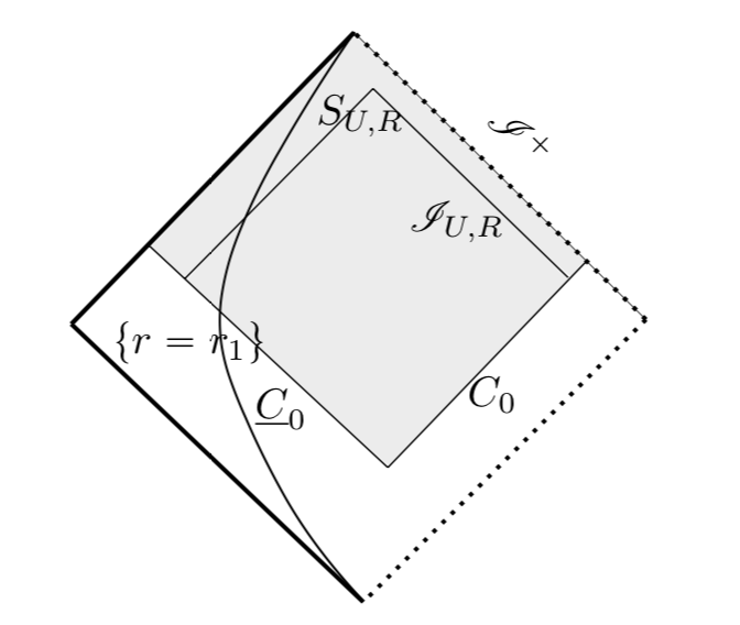
Figure 2: Penrose diagram of Reissner-Nordström spacetime with the sphere $S_{U,R}$ and the null hypersurface $\mathscr{I}_{U,R}$

Consider Reissner-Nordström spacetime with Bondi coordinates $(u,r,\theta,\phi)$. Let $S_{U,R}$ be the sphere obtained as the intersection of the hypersurfaces $\{u=U\}$ and $\{r=R\}$ for some $U$ and $R$ such that $R\gg r_{0}$, where $r_{0}$ is the radius of $S_{0}$, and $U\gg u_{0}$. Denote $\mathscr{I}_{U,R}$ the null hypersurface obtained as the ingoing past of $S_{U,R}$.

The characterization of this gauge normalization is related to two new quantities that we define here. We define the charge aspect function of a solution $\mathscr{S}$ as the scalar function obtained in the following way:

$$\check{\nu}=r^{4}\left(\mbox{div}\mkern-19.0mu/\,\,\,\,\zeta+2\,^{(F)}\rho\check{\,{}^{(F)}\rho}\right)$$ (211)

The above definition has a similar structure than the mass aspect function in vacuum spacetimes, but only depends on the charge of the spacetime (encoded in $\check{\,{}^{(F)}\rho}$). This quantity plays a fundamental role in the derivation of the decay for the projection to the $\ell=1$ spherical harmonics, which the electromagnetic tensor is responsible for.

We also define the mass-charge aspect function of a solution $\mathscr{S}$ as the scalar function obtained in the following way:

$$\check{\mu}=r^{3}\left(\mbox{div}\mkern-19.0mu/\,\,\,\,\zeta+\check{\rho}-4\,^{(F)}\rho\check{\,{}^{(F)}\rho}\right)-2r^{4}\,{}^{(F)}\rho\mbox{div}\mkern-19.0mu/\,\,\,\,\,^{(F)}\beta$$ (212)

Notice that the above definition reduces to the mass aspect function in the absence of an electromagnetic tensor, i.e. $\,{}^{(F)}\rho=\,^{(F)}\beta=0$. In the case of an electrovacuum spacetime, the function $\check{\mu}$ depends on both the mass (encoded into $\check{\rho}$) and the charge (encoded into $\check{\,{}^{(F)}\rho}$). This generalization plays a fundamental role in the derivation of decay in Section 12.4.3.

Both quantities, $\check{\nu}$ and $\check{\mu}$ verify well-behaved transport equations in the $e_{4}$ direction, which is the main reason why they are crucial in the derivation of decay. The derivation of the equations is obtained in Section A.3 of the Appendix.

We can now define the notion of $S_{U,R}$-normalization.

Definition 10.2.

Consider a seed data set as in Definition 9.1 and let $\mathscr{S}$ be the resulting solution given by Theorem 9.1. Suppose that $\mathscr{S}$ is bounded at $S_{U,R}$ for some $U$ and $R$. We say that $\mathscr{S}$ is $S_{U,R}$-normalized if

• the following conditions hold along the null hypersurface $\mathscr{I}_{U,R}$:

  1. For the projection to the $\ell=1$ spherical harmonics:

     $$\check{\kappa}_{\ell=1} = 0$$ (213)

     $$\check{\underline{\kappa}}_{\ell=1} = 0$$ (214)

     $$\check{\nu}_{\ell=1} = 0$$ (215)

     $$\mbox{div}\mkern-19.0mu/\,\,\,\,\underline{b}_{\ell=1} = 0$$ (216)

     where $\check{\nu}$ is the charge aspect function, as defined in (211).

  2. For the projection to the $\ell\geq 2$ spherical harmonics:

     $$\,{\mathcal{D}}{\,{}^{\star}\mkern-2.0mu}\mkern-16.0mu/_{2}\,{\mathcal{D}}{\,{}^{\star}\mkern-2.0mu}\mkern-16.0mu/_{1}(\check{\kappa},0) = 0$$ (217)

     $$\,{\mathcal{D}}{\,{}^{\star}\mkern-2.0mu}\mkern-16.0mu/_{2}\,{\mathcal{D}}{\,{}^{\star}\mkern-2.0mu}\mkern-16.0mu/_{1}(\check{\underline{\kappa}},0) = 0$$ (218)

     $$\,{\mathcal{D}}{\,{}^{\star}\mkern-2.0mu}\mkern-16.0mu/_{2}\,{\mathcal{D}}{\,{}^{\star}\mkern-2.0mu}\mkern-16.0mu/_{1}(\check{\mu},0) = 0$$ (219)

     $$\,{\mathcal{D}}{\,{}^{\star}\mkern-2.0mu}\mkern-16.0mu/_{2}\underline{b} = 0$$ (220)

     where $\check{\mu}$ is the mass-charge aspect function, as defined in (212).

• the following conditions hold on the sphere $S_{U,R}$:

  $$\check{\mbox{tr}_{\gamma}\not{g}}_{\ell=1} = 0$$ (221)

  $$\hat{\not{g}} = 0$$ (222)

We denote such solutions by $\mathscr{S}^{U,R}$.

We immediately note the following.

Proposition 10.2.1.

The linearized Kerr-Newman solutions $\mathscr{K}$ of Definition 6.1 are $S_{U,R}$-normalized for every $U$ and $R$.

10.3 Achieving the initial data normalization for a general $\mathscr{S}$

In this section, we prove the existence of a pure gauge solution $\mathscr{G}^{id}$ such that upon subtracting this to a given $\mathscr{S}$ arising from smooth seed data, the resulting solution is generated by data satisfying all conditions of Definition 10.1.

Theorem 10.1.

Consider a seed data set as in Definition 9.1 and let $\mathscr{S}$ be the resulting solution given by Theorem 9.1. Then there exists a pure gauge solution $\mathscr{G}^{id}$, explicitly computable from the seed data of $\mathscr{S}$, such that

$$\mathscr{S}^{id}:=\mathscr{S}-\mathscr{G}^{id}$$

is initial data normalized. The pure gauge solution $\mathscr{G}^{id}$ is unique and arises itself from the seed data.

Proof.

To identify the pure gauge solution $\mathscr{G}^{id}$, it suffices to identify the functions $h,\underline{h},a,c,d,l,q_{1},q_{2}$ as in Lemmas 6.1.5 and 6.1.6. In particular, we will make use of the conditions in Definition 10.1 to determine those functions and their derivative along the $e_{3}$ direction, and then we make use of the transport equations required in Lemmas 6.1.5 and 6.1.6 to extend those functions in the whole spacetime along the $e_{4}$ direction. Using the orthogonal decomposition in spherical harmonics, we can treat the projection to the $\ell=0$, $\ell=1$ and $\ell\geq 2$ spherical harmonics separately. This procedure uniquely determines the pure gauge solution $\mathscr{G}^{id}$ globally in the spacetime.

Projection to the $\ell=0$ spherical harmonics - achieving (199), (200), (201). Recall that the functions in the definition of pure gauge solutions which are supported in $\ell=0$ spherical harmonics are $c$, $d$ and $l$. We denote $\kappa^{\tiny(1)}_{0}$, $\underline{\kappa}^{\tiny(1)}_{0}$, $\varsigma^{\tiny(1)}_{0}$ and $\underline{\Omega}^{\tiny(1)}_{0}$ the functions determined on $\underline{C}_{0}$ by the seed initial data set.

We define along $\underline{C}_{0}$ the following function:

$$c := \frac{r}{2}\kappa^{\tiny(1)}_{0},\qquad d:=\varsigma^{\tiny(1)}_{0},\qquad l:=\frac{r}{2}\left(-\underline{\kappa}c-(\underline{\kappa}^{\tiny(1)}_{0}-\underline{\kappa}\underline{\Omega}^{\tiny(1)}_{0})\right)$$

Using Lemma 6.1.5, we see that the above conditions imply that $\mathscr{S}_{1}:=\mathscr{S}-\mathscr{G}_{0,0,c,d,l,0,0}$ verifies conditions (199), (200), (201) on $\underline{C}_{0}$. The transport equations (172) and (173) imply that $\partial_{r}c(u,r)=\partial_{r}d(u,r)=0$, therefore $c(u,r)=c(u)$ and $d(u,r)=d(r)$. This implies that the above definition of $c$ and $d$ along $\underline{C}_{0}$ determines $c$ and $d$ globally. Once $c$ is globally determined, the transport equation (174) globally determines $l$. Therefore $c,d,l$ are uniquely determined.

The following choice of pure gauge solutions will be supported in $\ell\geq 1$, and therefore will not change conditions (199), (200), (201).

Projection to the $\ell=1$ spherical harmonics - achieving (202), (203) and (204). We identify globally the projection to the $\ell=1$ spherical harmonics of $a$, $h$ and $\underline{h}$. We denote $\check{\kappa}_{0}$, $\,{}^{(F)}\beta_{0}$, $\,{}^{(F)}\underline{\beta}_{0}$ the functions on $S_{0}$ which are part of the seed initial data.

We define on $S_{0}$ the following functions:

$$h_{\ell=1} := \frac{r_{0}^{4}}{2Q}{\mbox{div}\mkern-19.0mu/\,\,\,\,\,^{(F)}\beta_{0}}_{\ell=1}$$

$$\underline{h}_{\ell=1} := -\frac{r_{0}^{4}}{2Q}{\mbox{div}\mkern-19.0mu/\,\,\,\,\,^{(F)}\underline{\beta}_{0}}_{\ell=1}$$

$$a_{\ell=1} = \frac{r_{0}}{2}\left({\check{\kappa}}_{\ell=1}-\frac{2}{r_{0}^{2}}h_{\ell=1}-\left(\frac{1}{4}\kappa(r_{0})\underline{\kappa}(r_{0})\right)h_{\ell=1}-\frac{1}{4}\kappa(r_{0})^{2}\underline{h}_{\ell=1}\right)$$

Using Lemma 6.1.5, we see that the above conditions imply that $\mathscr{S}_{2}:=\mathscr{S}_{1}-\mathscr{G}_{h_{\ell=1},\underline{h}_{\ell=1},a_{\ell=1},0,0}$ verifies conditions $\check{\kappa}_{\ell=1}=\mbox{div}\mkern-19.0mu/\,\,\,\,\,^{(F)}\beta_{\ell=1}=\mbox{div}\mkern-19.0mu/\,\,\,\,\,^{(F)}\underline{\beta}_{\ell=1}=0$ on $S_{0}$.

In order to obtain the cancellation along $\underline{C}_{0}$, we impose transport equations for $h_{\ell=1}$, $\underline{h}_{\ell=1}$ and $a_{\ell=1}$. In particular, we have along $\underline{C}_{0}$:

$$\nabla\mkern-13.0mu/\,_{3}\left(\frac{2Q}{r^{4}}h_{\ell=1}\right)=\nabla\mkern-13.0mu/\,_{3}\mbox{div}\mkern-19.0mu/\,\,\,\,\,^{(F)}\beta_{\ell=1}[\mathscr{S}]$$

$$\nabla\mkern-13.0mu/\,_{3}\left(\frac{2Q}{r^{4}}\underline{h}_{\ell=1}\right)=-\nabla\mkern-13.0mu/\,_{3}\mbox{div}\mkern-19.0mu/\,\,\,\,\,^{(F)}\underline{\beta}_{\ell=1}[\mathscr{S}]$$

The above transport equations together with the above initial conditions uniquely determine $h_{\ell=1}$ and $\underline{h}_{\ell=1}$ along $\underline{C}_{0}$. We similarly impose the $e_{3}$ derivative of $a_{\ell=1}$ to coincide with the derivative of the right hand side of the above definition.

Transport equation (170) then uniquely determines $h_{\ell=1}$ globally. The transport equation (169) determines $a_{\ell=1}$ globally. Then transport equation (171) uniquely determines the value of $\underline{h}_{\ell=1}$ globally. This implies that $\mathscr{S}_{2}$ verifies conditions (202), (203) and (204).

Projection to the $\ell\geq 2$ spherical harmonics - achieving (206), (207) and (208). We identify globally the projection to the $\ell\geq 2$ spherical harmonics of $h$, $\underline{h}$ and $a$. We denote $\,{\mathcal{D}}{\,{}^{\star}\mkern-2.0mu}\mkern-16.0mu/_{2}\,{\mathcal{D}}{\,{}^{\star}\mkern-2.0mu}\mkern-16.0mu/_{1}(\check{\kappa}_{0},0)$, $\widehat{\chi}_{0}$, $\widehat{\underline{\chi}}_{0}$ the symmetric traceless $2$-tensors on $S_{0}$ which are determined by the seed initial data.

We define on $S_{0}$ the following symmetric traceless $2$-tensors:

$$\,{\mathcal{D}}{\,{}^{\star}\mkern-2.0mu}\mkern-16.0mu/_{2}\,{\mathcal{D}}{\,{}^{\star}\mkern-2.0mu}\mkern-16.0mu/_{1}(h,0) := -\widehat{\chi}_{0}$$

$$\,{\mathcal{D}}{\,{}^{\star}\mkern-2.0mu}\mkern-16.0mu/_{2}\,{\mathcal{D}}{\,{}^{\star}\mkern-2.0mu}\mkern-16.0mu/_{1}(\underline{h},0) := -\widehat{\underline{\chi}}_{0}$$

$$\,{\mathcal{D}}{\,{}^{\star}\mkern-2.0mu}\mkern-16.0mu/_{2}\,{\mathcal{D}}{\,{}^{\star}\mkern-2.0mu}\mkern-16.0mu/_{1}(a,0) := \frac{r_{0}}{2}\big{(}\,{\mathcal{D}}{\,{}^{\star}\mkern-2.0mu}\mkern-16.0mu/_{2}\,{\mathcal{D}}{\,{}^{\star}\mkern-2.0mu}\mkern-16.0mu/_{1}(\check{\kappa}_{0},0)-2\,{\mathcal{D}}{\,{}^{\star}\mkern-2.0mu}\mkern-16.0mu/_{2}\,{\mathcal{D}}\mkern-8.0mu/_{2}(\,{\mathcal{D}}{\,{}^{\star}\mkern-2.0mu}\mkern-16.0mu/_{2}\,{\mathcal{D}}{\,{}^{\star}\mkern-2.0mu}\mkern-16.0mu/_{1}(h,0))+\frac{2}{r_{0}^{2}}\,{\mathcal{D}}{\,{}^{\star}\mkern-2.0mu}\mkern-16.0mu/_{2}\,{\mathcal{D}}{\,{}^{\star}\mkern-2.0mu}\mkern-16.0mu/_{1}(h,0)$$

$$-\left(\frac{1}{4}\kappa(r_{0})\underline{\kappa}(r_{0})\right)\,{\mathcal{D}}{\,{}^{\star}\mkern-2.0mu}\mkern-16.0mu/_{2}\,{\mathcal{D}}{\,{}^{\star}\mkern-2.0mu}\mkern-16.0mu/_{1}(h,0)-\frac{1}{4}\kappa(r_{0})^{2}\,{\mathcal{D}}{\,{}^{\star}\mkern-2.0mu}\mkern-16.0mu/_{2}\,{\mathcal{D}}{\,{}^{\star}\mkern-2.0mu}\mkern-16.0mu/_{1}(\underline{h},0)\big{)}$$

By Lemma 4.3.1, the above conditions uniquely determine the projection to the $\ell\geq 2$ spherical modes of $h$, $\underline{h}$ and $a$ on $S_{0}$. Using Lemma 6.1.5, we see that the above conditions imply that $\mathscr{S}_{3}:=\mathscr{S}_{2}-\mathscr{G}_{h_{\ell\geq 2},\underline{h}_{\ell\geq 2},a_{\ell\geq 2},0,0}$ verifies conditions $\,{\mathcal{D}}{\,{}^{\star}\mkern-2.0mu}\mkern-16.0mu/_{2}\,{\mathcal{D}}{\,{}^{\star}\mkern-2.0mu}\mkern-16.0mu/_{1}(\check{\kappa},0)=\chi=\underline{\chi}=0$ on $S_{0}$.

Applying the $e_{3}$ derivative to the above definitions we derive transport equations for $\,{\mathcal{D}}{\,{}^{\star}\mkern-2.0mu}\mkern-16.0mu/_{2}\,{\mathcal{D}}{\,{}^{\star}\mkern-2.0mu}\mkern-16.0mu/_{1}(h,0)$, $\,{\mathcal{D}}{\,{}^{\star}\mkern-2.0mu}\mkern-16.0mu/_{2}\,{\mathcal{D}}{\,{}^{\star}\mkern-2.0mu}\mkern-16.0mu/_{1}(\underline{h},0)$ and $\,{\mathcal{D}}{\,{}^{\star}\mkern-2.0mu}\mkern-16.0mu/_{2}\,{\mathcal{D}}{\,{}^{\star}\mkern-2.0mu}\mkern-16.0mu/_{1}(a,0)$ which uniquely determine them on $\underline{C}_{0}$. Then transport equation (170) then uniquely determines $\,{\mathcal{D}}{\,{}^{\star}\mkern-2.0mu}\mkern-16.0mu/_{2}\,{\mathcal{D}}{\,{}^{\star}\mkern-2.0mu}\mkern-16.0mu/_{1}(h,0)$ globally and transport equation (169) determines $\,{\mathcal{D}}{\,{}^{\star}\mkern-2.0mu}\mkern-16.0mu/_{2}\,{\mathcal{D}}{\,{}^{\star}\mkern-2.0mu}\mkern-16.0mu/_{1}(a,0)$ globally. Then transport equation (171) uniquely determines the value of $\,{\mathcal{D}}{\,{}^{\star}\mkern-2.0mu}\mkern-16.0mu/_{2}\,{\mathcal{D}}{\,{}^{\star}\mkern-2.0mu}\mkern-16.0mu/_{1}(\underline{h},0)$ globally. Again by Lemma 4.3.1, the above conditions uniquely determine the projection to the $\ell\geq 2$ spherical modes of $h$, $\underline{h}$ and $a$ globally. This implies that $\mathscr{S}_{3}$ verifies in addition conditions (206), (207) and (208).

Conditions on the metric coefficients - achieving (205), (209) and (210). With the above, we exhausted the freedom of using Lemma 6.1.5, since we globally determined the functions $h$, $\underline{h}$, $a$ and $\lambda$. In particular, the above choices also modified $\hat{\not{g}}$, $\underline{b}$ and $\check{\mbox{tr}_{\gamma}\not{g}}$ on $\underline{C}_{0}$, which now differ from the one given by the seed initial data. In what follows we will achieve the remaining conditions of Definition 10.1 using pure gauge solutions of the form $\mathscr{G}_{0,0,0,q_{1},q_{2}}$ as in Lemma 6.1.6. Observe that these solutions have all components different from $\hat{\not{g}}$, $\underline{b}$ and $\check{\mbox{tr}_{\gamma}\not{g}}$ vanishing, and therefore do not modify the achieved conditions above.

We identify $q_{1}$ and $q_{2}$ on $S_{0}$. We define on $S_{0}$ the following:

$$(q_{1})_{\ell=1} = -\frac{1}{4r_{0}^{2}}\check{\mbox{tr}_{\gamma}\not{g}}_{l=1}[\mathscr{S}_{3}]|_{S_{0}},\qquad\,{\mathcal{D}}{\,{}^{\star}\mkern-2.0mu}\mkern-16.0mu/_{2}\,{\mathcal{D}}{\,{}^{\star}\mkern-2.0mu}\mkern-16.0mu/_{1}(q_{1},q_{2})=\frac{1}{2r_{0}^{2}}\hat{\not{g}}[\mathscr{S}_{3}]|_{S_{0}}$$

where we denote $\check{\mbox{tr}_{\gamma}\not{g}}_{\ell=1}[\mathscr{S}_{3}]|_{S_{0}}$ and $\hat{\not{g}}[\mathscr{S}_{3}]|_{S_{0}}$ the respective value of $\check{\mbox{tr}_{\gamma}\not{g}}_{\ell=1}$ and $\hat{\not{g}}$ of the solution $\mathscr{S}_{3}$ defined above on the initial sphere $S_{0}$. By the above discussion, these values only depend on initial seed data. By Lemma 4.3.1, the above conditions uniquely determine $q_{1}$ and $q_{2}$ on $S_{0}$.

Condition (205) on $\underline{C}_{0}$ determines a transport equation along $\underline{C}_{0}$ for $q_{1}$ and $q_{2}$:

$$r^{2}\,{\mathcal{D}}{\,{}^{\star}\mkern-2.0mu}\mkern-16.0mu/_{1}(\nabla\mkern-13.0mu/\,_{3}q_{1},\nabla\mkern-13.0mu/\,_{3}q_{2})^{A} = \underline{b}^{A}[\mathscr{S}_{3}]-\frac{1}{3}r^{3}\epsilon^{AB}\partial_{B}\left(2\check{\sigma}_{\ell=1}[\mathscr{S}_{3}]+\,^{(F)}\rho\check{\,{}^{(F)}\sigma}_{\ell=1}[\mathscr{S}_{3}]\right)$$

which together with (175) and (176) globally determine $q_{1}$ and $q_{2}$. The above conditions imply that $\mathscr{S}_{4}:=\mathscr{S}_{3}-\mathscr{G}_{0,0,0,q_{1},q_{2}}$ verifies in addition conditions (205), (209) and (210).

Define $\mathscr{G}^{id}:=\mathscr{G}_{h,\underline{h},a,c,d,l,0,0}+\mathscr{G}_{0,0,0,q_{1},q_{2}}$ with $h,\underline{h},a,q_{1},q_{2}$ determined as above. Then

$$\mathscr{S}^{id}:=\mathscr{S}-\mathscr{G}^{id}=\mathscr{S}_{4}$$

verifies all conditions of Definition 10.1 and is therefore initial data normalized. By construction, $\mathscr{G}^{id}$ is also uniquely determined. ∎

10.4 Achieving the $S_{U,R}$-normalization for a bounded $\mathscr{S}$

In this section, we prove the existence of a pure gauge solution $\mathscr{G}^{U,R}$ such that upon subtracting this to a given $\mathscr{S}$, which is assumed to be bounded at the sphere $S_{U,R}$ for some $U$ and $R$, the resulting solution satisfies all conditions of Definition 10.2. Observe that we do not need to modify the projection to the $\ell=0$ spherical harmonics because such projection is proved to vanish in Section 11.1.1.

Theorem 10.2.

Consider a seed data set as in Definition 9.1 and let $\mathscr{S}$ be the resulting solution given by Theorem 9.1. Suppose that the solution $\mathscr{S}$ is bounded at the sphere $S_{U,R}$.

Then there exists a pure gauge solution $\mathscr{G}^{U,R}$ supported in $\ell\geq 1$ spherical harmonics such that

$$\mathscr{S}^{U,R}:=\mathscr{S}-\mathscr{G}^{U,R}$$

is $S_{U,R}$-normalized. The pure gauge solution $\mathscr{G}^{U,R}$ is unique and is bounded by the initial data seed.

Proof.

We follow the same pattern as in the proof of Theorem 10.1. Since $\mathscr{G}^{U,R}$ is taken to be supported in $\ell\geq 1$ spherical harmonics it suffices to identify globally the functions $h$, $\underline{h}$ and $a$ with $a$ supported in $\ell\geq 1$, and $q_{1}$ and $q_{2}$. Again, we treat the projection to the $\ell=1$ and $\ell\geq 2$ separately.

Projection to the $\ell=1$ spherical harmonics - achieving (213), (214), (215). We identify globally the projection to the $\ell=1$ spherical harmonics of $a$, $h$ and $\underline{h}$. According to Lemma 6.1.5, for a pure gauge solution the components $\check{\kappa}$ and $\check{\underline{\kappa}}$ verify

$$\check{\kappa} = \kappa a+\,{\mathcal{D}}\mkern-8.0mu/_{1}\,{\mathcal{D}}{\,{}^{\star}\mkern-2.0mu}\mkern-16.0mu/_{1}(h,0)+\frac{1}{4}\kappa\underline{\kappa}h+\frac{1}{4}\kappa^{2}\underline{h}$$ (223)

$$\check{\underline{\kappa}} = -\underline{\kappa}a+\,{\mathcal{D}}\mkern-8.0mu/_{1}\,{\mathcal{D}}{\,{}^{\star}\mkern-2.0mu}\mkern-16.0mu/_{1}(\underline{h},0)+\left(\frac{1}{4}\underline{\kappa}^{2}+{\underline{\omega}}\underline{\kappa}\right)h+\left(\frac{1}{4}\kappa\underline{\kappa}-\rho\right)\underline{h}$$ (224)

Multiplying (223) by $\underline{\kappa}$ and (224) by $\kappa$ and summing them we obtain:

$$\,{\mathcal{D}}\mkern-8.0mu/_{1}\,{\mathcal{D}}{\,{}^{\star}\mkern-2.0mu}\mkern-16.0mu/_{1}(\underline{\kappa}h+\kappa\underline{h},0)+\left(\frac{1}{2}\kappa\underline{\kappa}+{\underline{\omega}}\kappa\right)\underline{\kappa}h+\left(\frac{1}{2}\kappa\underline{\kappa}-\rho\right)\kappa\underline{h} = \underline{\kappa}\check{\kappa}+\kappa\check{\underline{\kappa}}$$

Setting $z=\underline{\kappa}h+\kappa\underline{h}$ and observing that ${\underline{\omega}}\kappa=-\rho$ in the background we obtain for a pure gauge solution

$$\,{\mathcal{D}}\mkern-8.0mu/_{1}\,{\mathcal{D}}{\,{}^{\star}\mkern-2.0mu}\mkern-16.0mu/_{1}(z,0)+\left(\frac{1}{2}\kappa\underline{\kappa}-\rho\right)z = \underline{\kappa}\check{\kappa}+\kappa\check{\underline{\kappa}}$$ (225)

Projecting the above equation to the $\ell=1$ spherical harmonics, using that $\,{\mathcal{D}}\mkern-8.0mu/_{1}\,{\mathcal{D}}{\,{}^{\star}\mkern-2.0mu}\mkern-16.0mu/_{1}=-\mbox{$\bigtriangleup\mkern-13.0mu/\,$}$ and using the Gauss equation (40), we obtain an equation for $z_{\ell=1}$:

$$\left(-3\rho+2\,^{(F)}\rho^{2}\right)z_{\ell=1} = \underline{\kappa}\check{\kappa}[\mathscr{S}]_{\ell=1}+\kappa\check{\underline{\kappa}}[\mathscr{S}]_{l=1}$$ (226)

The above determines the value of $z_{\ell=1}$ along the null hypersurface $\mathscr{I}_{U,R}$. Multiplying (223) by $\underline{\kappa}$ and (224) by $\kappa$ and subtracting them we obtain:

$$2\underline{\kappa}\kappa a+\,{\mathcal{D}}\mkern-8.0mu/_{1}\,{\mathcal{D}}{\,{}^{\star}\mkern-2.0mu}\mkern-16.0mu/_{1}(\underline{\kappa}h-\kappa\underline{h},0)-{\underline{\omega}}\kappa\underline{\kappa}h+\rho\kappa\underline{h} = \underline{\kappa}\check{\kappa}-\kappa\check{\underline{\kappa}}$$

Setting $\overline{z}=\underline{\kappa}h-\kappa\underline{h}$ and observing that ${\underline{\omega}}\kappa=-\rho$ we obtain for a pure gauge solution

$$\,{\mathcal{D}}\mkern-8.0mu/_{1}\,{\mathcal{D}}{\,{}^{\star}\mkern-2.0mu}\mkern-16.0mu/_{1}(\overline{z},0)+2\kappa\underline{\kappa}a = \underline{\kappa}\check{\kappa}-\kappa\check{\underline{\kappa}}-\rho z$$ (227)

According to Lemma 6.1.5, for a pure gauge solution the component $\check{\nu}$ verifies

$$r^{-4}\check{\nu} = \left(-\frac{1}{4}\underline{\kappa}-{\underline{\omega}}\right)\,{\mathcal{D}}\mkern-8.0mu/_{1}\,{\mathcal{D}}{\,{}^{\star}\mkern-2.0mu}\mkern-16.0mu/_{1}(h,0)+\frac{1}{4}\kappa\,{\mathcal{D}}\mkern-8.0mu/_{1}\,{\mathcal{D}}{\,{}^{\star}\mkern-2.0mu}\mkern-16.0mu/_{1}(\underline{h},0)+\,{\mathcal{D}}\mkern-8.0mu/_{1}\,{\mathcal{D}}{\,{}^{\star}\mkern-2.0mu}\mkern-16.0mu/_{1}(a,0)+\,^{(F)}\rho^{2}(\underline{\kappa}h+\kappa\underline{h})$$

which can be written in terms of $z$ and $\overline{z}$ as

$$r^{-4}\check{\nu} = \left(-\frac{1}{4}\underline{\kappa}+\frac{1}{4}\rho r\right)\underline{\kappa}^{-1}\,{\mathcal{D}}\mkern-8.0mu/_{1}\,{\mathcal{D}}{\,{}^{\star}\mkern-2.0mu}\mkern-16.0mu/_{1}(\overline{z},0)+\,{\mathcal{D}}\mkern-8.0mu/_{1}\,{\mathcal{D}}{\,{}^{\star}\mkern-2.0mu}\mkern-16.0mu/_{1}(a,0)+\frac{1}{4}\rho r\underline{\kappa}^{-1}\,{\mathcal{D}}\mkern-8.0mu/_{1}\,{\mathcal{D}}{\,{}^{\star}\mkern-2.0mu}\mkern-16.0mu/_{1}(z,0)+\,^{(F)}\rho^{2}z$$

Multiplying the above by $\underline{\kappa}$ and observing that $-\frac{1}{4}\underline{\kappa}+\frac{1}{4}r\rho=\frac{1}{2r}\left(1-\frac{3M}{r}+\frac{2Q^{2}}{r^{2}}\right)$ we obtain

$$\begin{split}\underline{\kappa}r^{-4}\check{\nu}&=\left(-\frac{1}{4}\underline{\kappa}+\frac{1}{4}\rho r\right)\,{\mathcal{D}}\mkern-8.0mu/_{1}\,{\mathcal{D}}{\,{}^{\star}\mkern-2.0mu}\mkern-16.0mu/_{1}(\overline{z},0)+\underline{\kappa}\,{\mathcal{D}}\mkern-8.0mu/_{1}\,{\mathcal{D}}{\,{}^{\star}\mkern-2.0mu}\mkern-16.0mu/_{1}(a,0)+\frac{1}{4}\rho r\,{\mathcal{D}}\mkern-8.0mu/_{1}\,{\mathcal{D}}{\,{}^{\star}\mkern-2.0mu}\mkern-16.0mu/_{1}(z,0)+\underline{\kappa}\,^{(F)}\rho^{2}z\end{split}$$ (228)

If $R\gg 3M$, then, along $\mathscr{I}_{U,R}$, $r\gg 3M$ and therefore we can safely multiply (227) by $\frac{1}{2r}\left(1-\frac{3M}{r}+\frac{2Q^{2}}{r^{2}}\right)$ and subtract (228) to obtain:

$$\begin{split}&\,{\mathcal{D}}\mkern-8.0mu/_{1}\,{\mathcal{D}}{\,{}^{\star}\mkern-2.0mu}\mkern-16.0mu/_{1}(a,0)+\left(\frac{1}{2}\kappa\underline{\kappa}-\rho+4\,^{(F)}\rho^{2}\right)a\\ &=r^{-4}\check{\nu}-\frac{1}{2r}\left(1-\frac{3M}{r}+\frac{2Q^{2}}{r^{2}}\right)\check{\kappa}+\frac{1}{2r}\left(1-\frac{3M}{r}+\frac{2Q^{2}}{r^{2}}\right)\underline{\kappa}^{-1}\kappa\check{\underline{\kappa}}\\ &-\left(\frac{1}{4}r\rho\right)\underline{\kappa}^{-1}\,{\mathcal{D}}\mkern-8.0mu/_{1}\,{\mathcal{D}}{\,{}^{\star}\mkern-2.0mu}\mkern-16.0mu/_{1}(z,0)-\left(\,{}^{(F)}\rho^{2}-\frac{1}{2r}\left(1-\frac{3M}{r}+\frac{2Q^{2}}{r^{2}}\right)\rho\underline{\kappa}^{-1}\right)z\end{split}$$ (229)

Projecting to the $\ell=1$ spherical harmonics we see that the right hand side of (229) is already determined by (226). This gives in particular

$$\begin{split}\left(-3\rho+6\,^{(F)}\rho^{2}\right)a_{\ell=1}&=r^{-4}\check{\nu}[\mathscr{S}]_{\ell=1}-\frac{1}{2r}\left(1-\frac{3M}{r}+\frac{2Q^{2}}{r^{2}}\right)\check{\kappa}[\mathscr{S}]_{\ell=1}\\ &+\frac{1}{2r}\left(1-\frac{3M}{r}+\frac{2Q^{2}}{r^{2}}\right)\underline{\kappa}^{-1}\kappa\check{\underline{\kappa}}[\mathscr{S}]_{\ell=1}\\ &-\left(\frac{1}{4}r\rho\right)\underline{\kappa}^{-1}2Kz_{\ell=1}-\left(\,{}^{(F)}\rho^{2}-\frac{1}{2r}\left(1-\frac{3M}{r}+\frac{2Q^{2}}{r^{2}}\right)\rho\underline{\kappa}^{-1}\right)z_{\ell=1}\end{split}$$ (230)

with known right hand side along $\mathscr{I}_{U,R}$. This determines $a_{\ell=1}$ along $\mathscr{I}_{U,R}$. Finally the projection of (227) to the $\ell=1$ spherical harmonics determines $\overline{z}_{\ell=1}$:

$$\frac{2}{r^{2}}\overline{z}_{\ell=1} = -2\kappa\underline{\kappa}a_{\ell=1}\underline{\kappa}\check{\kappa}[\mathscr{S}]_{\ell=1}-\kappa\check{\underline{\kappa}}[\mathscr{S}]_{\ell=1}-\rho z_{\ell=1}$$

The value of $z_{\ell=1}$ and $\overline{z}_{\ell=1}$ uniquely determine the value of $h_{\ell=1}$ and $\underline{h}_{\ell=1}$ along $\mathscr{I}_{U,R}$. Transport equation (170) uniquely determines $h_{\ell=1}$ globally, transport equation (169) determines $a_{\ell=1}$ globally and finally transport equation (171) uniquely determines the value of $\underline{h}_{\ell=1}$ globally. This implies that $\mathscr{S}-\mathscr{G}_{h_{\ell=1},\underline{h}_{\ell=1},a_{\ell=1},0,0}$ verifies conditions (213), (214), (215).

Projection to the $\ell\geq 2$ spherical harmonics - achieving (217), (218) and (219). We identify globally the projection to the $\ell\geq 2$ spherical harmonics of $a$, $h$ and $\underline{h}$. We first derive some preliminary relations.

According to Lemma 6.1.5, for a pure gauge solution the component $\check{\mu}$ verifies

$$r^{-3}\check{\mu} = \left(-\frac{1}{4}\underline{\kappa}-{\underline{\omega}}-2r\,^{(F)}\rho^{2}\right)\,{\mathcal{D}}\mkern-8.0mu/_{1}\,{\mathcal{D}}{\,{}^{\star}\mkern-2.0mu}\mkern-16.0mu/_{1}(h,0)+\frac{1}{4}\kappa\,{\mathcal{D}}\mkern-8.0mu/_{1}\,{\mathcal{D}}{\,{}^{\star}\mkern-2.0mu}\mkern-16.0mu/_{1}(\underline{h},0)+\,{\mathcal{D}}\mkern-8.0mu/_{1}\,{\mathcal{D}}{\,{}^{\star}\mkern-2.0mu}\mkern-16.0mu/_{1}(a,0)$$

$$+\left(\frac{3}{4}\rho-\frac{3}{2}\,^{(F)}\rho^{2}\right)(\underline{\kappa}h+\kappa\underline{h})$$

which can be written in terms of $z$ and $\overline{z}$ as

$$r^{-3}\check{\mu} = \left(-\frac{1}{4}\underline{\kappa}+\frac{1}{4}r\rho-r\,^{(F)}\rho^{2}\right)\underline{\kappa}^{-1}\,{\mathcal{D}}\mkern-8.0mu/_{1}\,{\mathcal{D}}{\,{}^{\star}\mkern-2.0mu}\mkern-16.0mu/_{1}(\overline{z},0)+\left(\frac{1}{4}r\rho-r\,^{(F)}\rho^{2}\right)\underline{\kappa}^{-1}\,{\mathcal{D}}\mkern-8.0mu/_{1}\,{\mathcal{D}}{\,{}^{\star}\mkern-2.0mu}\mkern-16.0mu/_{1}(z,0)$$

$$+\left(\frac{3}{4}\rho-\frac{3}{2}\,^{(F)}\rho^{2}\right)z+\,{\mathcal{D}}\mkern-8.0mu/_{1}\,{\mathcal{D}}{\,{}^{\star}\mkern-2.0mu}\mkern-16.0mu/_{1}(a,0)$$

Multiplying the above by $\underline{\kappa}$ and observing that $-\frac{1}{4}\underline{\kappa}+\frac{1}{4}r\rho-r\,^{(F)}\rho^{2}=\frac{1}{2r}\left(1-\frac{3M}{r}\right)$ we obtain

$$\begin{split}\underline{\kappa}r^{-3}\check{\mu}&=\frac{1}{2r}\left(1-\frac{3M}{r}\right)\,{\mathcal{D}}\mkern-8.0mu/_{1}\,{\mathcal{D}}{\,{}^{\star}\mkern-2.0mu}\mkern-16.0mu/_{1}(\overline{z},0)+\left(\frac{1}{4}r\rho-r\,^{(F)}\rho^{2}\right)\,{\mathcal{D}}\mkern-8.0mu/_{1}\,{\mathcal{D}}{\,{}^{\star}\mkern-2.0mu}\mkern-16.0mu/_{1}(z,0)+\left(\frac{3}{4}\rho-\frac{3}{2}\,^{(F)}\rho^{2}\right)\underline{\kappa}z\\ &+\underline{\kappa}\,{\mathcal{D}}\mkern-8.0mu/_{1}\,{\mathcal{D}}{\,{}^{\star}\mkern-2.0mu}\mkern-16.0mu/_{1}(a,0)\end{split}$$ (231)

If $R\gg 3M$, then, along $\mathscr{I}_{U,R}$, $r\gg 3M$ and therefore we can safely multiply (227) by $\frac{1}{2r}\left(1-\frac{3M}{r}\right)$ and subtract (231) to obtain:

$$\begin{split}\,{\mathcal{D}}\mkern-8.0mu/_{1}\,{\mathcal{D}}{\,{}^{\star}\mkern-2.0mu}\mkern-16.0mu/_{1}(a,0)+\left(\frac{1}{2}\kappa\underline{\kappa}-\rho+4\,^{(F)}\rho^{2}\right)a&=r^{-3}\check{\mu}-\frac{1}{2r}\left(1-\frac{3M}{r}\right)\check{\kappa}+\frac{1}{2r}\left(1-\frac{3M}{r}\right)\underline{\kappa}^{-1}\kappa\check{\underline{\kappa}}\\ &-\left(\frac{1}{4}r\rho-r\,^{(F)}\rho^{2}\right)\underline{\kappa}^{-1}\,{\mathcal{D}}\mkern-8.0mu/_{1}\,{\mathcal{D}}{\,{}^{\star}\mkern-2.0mu}\mkern-16.0mu/_{1}(z,0)\\ &-\left(\frac{3}{4}\rho-\frac{3}{2}\,^{(F)}\rho^{2}-\frac{1}{2r}\left(1-\frac{3M}{r}\right)\rho\underline{\kappa}^{-1}\right)z\end{split}$$ (232)

To verify conditions (217), (218) and (219) we are interested in determining $\,{\mathcal{D}}{\,{}^{\star}\mkern-2.0mu}\mkern-16.0mu/_{2}\,{\mathcal{D}}{\,{}^{\star}\mkern-2.0mu}\mkern-16.0mu/_{1}(z,0)$, $\,{\mathcal{D}}{\,{}^{\star}\mkern-2.0mu}\mkern-16.0mu/_{2}\,{\mathcal{D}}{\,{}^{\star}\mkern-2.0mu}\mkern-16.0mu/_{1}(\overline{z},0)$ and $\,{\mathcal{D}}{\,{}^{\star}\mkern-2.0mu}\mkern-16.0mu/_{2}\,{\mathcal{D}}{\,{}^{\star}\mkern-2.0mu}\mkern-16.0mu/_{1}(a,0)$ on $\mathscr{I}_{U,R}$.

We apply the operator $\,{\mathcal{D}}{\,{}^{\star}\mkern-2.0mu}\mkern-16.0mu/_{2}\,{\mathcal{D}}{\,{}^{\star}\mkern-2.0mu}\mkern-16.0mu/_{1}$ to (225), which translates in the following relation along $\mathscr{I}_{U,R}$:

$$\,{\mathcal{D}}{\,{}^{\star}\mkern-2.0mu}\mkern-16.0mu/_{2}\,{\mathcal{D}}{\,{}^{\star}\mkern-2.0mu}\mkern-16.0mu/_{1}\,{\mathcal{D}}\mkern-8.0mu/_{1}\,{\mathcal{D}}{\,{}^{\star}\mkern-2.0mu}\mkern-16.0mu/_{1}(z,0)+\left(\frac{1}{2}\kappa\underline{\kappa}-\rho\right)\,{\mathcal{D}}{\,{}^{\star}\mkern-2.0mu}\mkern-16.0mu/_{2}\,{\mathcal{D}}{\,{}^{\star}\mkern-2.0mu}\mkern-16.0mu/_{1}(z,0) = \underline{\kappa}\,{\mathcal{D}}{\,{}^{\star}\mkern-2.0mu}\mkern-16.0mu/_{2}\,{\mathcal{D}}{\,{}^{\star}\mkern-2.0mu}\mkern-16.0mu/_{1}(\check{\kappa}[\mathscr{S}],0)+\kappa\,{\mathcal{D}}{\,{}^{\star}\mkern-2.0mu}\mkern-16.0mu/_{2}\,{\mathcal{D}}{\,{}^{\star}\mkern-2.0mu}\mkern-16.0mu/_{1}(\check{\underline{\kappa}}[\mathscr{S}],0)$$

By (16) we have that

$$\,{\mathcal{D}}{\,{}^{\star}\mkern-2.0mu}\mkern-16.0mu/_{2}\,{\mathcal{D}}{\,{}^{\star}\mkern-2.0mu}\mkern-16.0mu/_{1}\,{\mathcal{D}}\mkern-8.0mu/_{1} = (2\,{\mathcal{D}}{\,{}^{\star}\mkern-2.0mu}\mkern-16.0mu/_{2}\,{\mathcal{D}}\mkern-8.0mu/_{2}+2K)\,{\mathcal{D}}{\,{}^{\star}\mkern-2.0mu}\mkern-16.0mu/_{2}$$ (233)

which therefore implies the following relation for $\,{\mathcal{D}}{\,{}^{\star}\mkern-2.0mu}\mkern-16.0mu/_{2}\,{\mathcal{D}}{\,{}^{\star}\mkern-2.0mu}\mkern-16.0mu/_{1}(z,0)$:

$$\left(2\,{\mathcal{D}}{\,{}^{\star}\mkern-2.0mu}\mkern-16.0mu/_{2}\,{\mathcal{D}}\mkern-8.0mu/_{2}+2K+\frac{1}{2}\kappa\underline{\kappa}-\rho\right)\,{\mathcal{D}}{\,{}^{\star}\mkern-2.0mu}\mkern-16.0mu/_{2}\,{\mathcal{D}}{\,{}^{\star}\mkern-2.0mu}\mkern-16.0mu/_{1}(z,0) = \underline{\kappa}\,{\mathcal{D}}{\,{}^{\star}\mkern-2.0mu}\mkern-16.0mu/_{2}\,{\mathcal{D}}{\,{}^{\star}\mkern-2.0mu}\mkern-16.0mu/_{1}(\check{\kappa}[\mathscr{S}],0)+\kappa\,{\mathcal{D}}{\,{}^{\star}\mkern-2.0mu}\mkern-16.0mu/_{2}\,{\mathcal{D}}{\,{}^{\star}\mkern-2.0mu}\mkern-16.0mu/_{1}(\check{\underline{\kappa}}[\mathscr{S}],0)$$

By Gauss equation, we have

$$2\,{\mathcal{D}}{\,{}^{\star}\mkern-2.0mu}\mkern-16.0mu/_{2}\,{\mathcal{D}}\mkern-8.0mu/_{2}+2K+\frac{1}{2}\kappa\underline{\kappa}-\rho = 2\,{\mathcal{D}}{\,{}^{\star}\mkern-2.0mu}\mkern-16.0mu/_{2}\,{\mathcal{D}}\mkern-8.0mu/_{2}+2\left(-\frac{1}{4}\kappa\underline{\kappa}-\rho+\,^{(F)}\rho^{2}\right)+\frac{1}{2}\kappa\underline{\kappa}-\rho=2\,{\mathcal{D}}{\,{}^{\star}\mkern-2.0mu}\mkern-16.0mu/_{2}\,{\mathcal{D}}\mkern-8.0mu/_{2}-3\rho+2\,^{(F)}\rho^{2}$$

Define $\mathcal{E}$ to be the operator $\mathcal{E}:=2\,{\mathcal{D}}{\,{}^{\star}\mkern-2.0mu}\mkern-16.0mu/_{2}\,{\mathcal{D}}\mkern-8.0mu/_{2}-3\rho+2\,^{(F)}\rho^{2}$ on symmetric traceless $2$-tensors. Then the above relation gives

$$\mathcal{E}(\,{\mathcal{D}}{\,{}^{\star}\mkern-2.0mu}\mkern-16.0mu/_{2}\,{\mathcal{D}}{\,{}^{\star}\mkern-2.0mu}\mkern-16.0mu/_{1}(z,0)) = \underline{\kappa}\,{\mathcal{D}}{\,{}^{\star}\mkern-2.0mu}\mkern-16.0mu/_{2}\,{\mathcal{D}}{\,{}^{\star}\mkern-2.0mu}\mkern-16.0mu/_{1}(\check{\kappa}[\mathscr{S}],0)+\kappa\,{\mathcal{D}}{\,{}^{\star}\mkern-2.0mu}\mkern-16.0mu/_{2}\,{\mathcal{D}}{\,{}^{\star}\mkern-2.0mu}\mkern-16.0mu/_{1}(\check{\underline{\kappa}}[\mathscr{S}],0)$$ (234)

We show that the operator $\mathcal{E}$ is coercive.

Lemma 10.4.1.

Let $\mathcal{E}$ be the operator defined as $\mathcal{E}:=2\,{\mathcal{D}}{\,{}^{\star}\mkern-2.0mu}\mkern-16.0mu/_{2}\,{\mathcal{D}}\mkern-8.0mu/_{2}-3\rho+2\,^{(F)}\rho^{2}$. For any symmetric traceless two tensor $\theta$ we have

$$\int_{S}\theta\cdot\mathcal{E}\theta\geq\frac{4}{r^{2}}\int_{S}|\theta|^{2}$$

Proof.

We compute

$$\int_{S}\theta\cdot\mathcal{E}\theta=\int_{S}\theta\cdot(2\,{\mathcal{D}}{\,{}^{\star}\mkern-2.0mu}\mkern-16.0mu/_{2}\,{\mathcal{D}}\mkern-8.0mu/_{2}-3\rho+2\,^{(F)}\rho^{2})\theta=\int_{S}2|\,{\mathcal{D}}\mkern-8.0mu/_{2}\theta|^{2}+(-3\rho+2\,^{(F)}\rho^{2})|\theta|^{2}$$

Using the standard Poincaré inequality on spheres and $\int_{S}|\nabla\mkern-13.0mu/\,\theta|^{2}+2K|\theta|^{2}=2\int_{S}|\,{\mathcal{D}}\mkern-8.0mu/_{2}\theta|^{2}$, we have that $\int_{S}|\,{\mathcal{D}}\mkern-8.0mu/_{2}\theta|^{2}\geq\int_{S}2K|\theta|^{2}$, and therefore

$$\int_{S}\theta\cdot\mathcal{E}\theta\geq\int_{S}\left(\frac{4}{r^{2}}+\frac{6M}{r^{3}}-\frac{4Q^{2}}{r^{4}}\right)|\theta|^{2}$$

Observe that $\frac{6M}{r^{3}}-\frac{4Q^{2}}{r^{4}}\geq\frac{2M^{2}}{r^{3}}$ for all $r>M$ and $|Q|<M$. We therefore obtain the inequality. ∎

The above Lemma shows that (234) uniquely determines $\,{\mathcal{D}}{\,{}^{\star}\mkern-2.0mu}\mkern-16.0mu/_{2}\,{\mathcal{D}}{\,{}^{\star}\mkern-2.0mu}\mkern-16.0mu/_{1}(z,0)$ along $\mathscr{I}_{U,R}$.

Applying the operator $\,{\mathcal{D}}{\,{}^{\star}\mkern-2.0mu}\mkern-16.0mu/_{2}\,{\mathcal{D}}{\,{}^{\star}\mkern-2.0mu}\mkern-16.0mu/_{1}$ to (232) we obtain on $\mathscr{I}_{U,R}$

$$\,{\mathcal{D}}{\,{}^{\star}\mkern-2.0mu}\mkern-16.0mu/_{2}\,{\mathcal{D}}{\,{}^{\star}\mkern-2.0mu}\mkern-16.0mu/_{1}\,{\mathcal{D}}\mkern-8.0mu/_{1}\,{\mathcal{D}}{\,{}^{\star}\mkern-2.0mu}\mkern-16.0mu/_{1}(a,0)+\left(\frac{1}{2}\kappa\underline{\kappa}-\rho+4\,^{(F)}\rho^{2}\right)\,{\mathcal{D}}{\,{}^{\star}\mkern-2.0mu}\mkern-16.0mu/_{2}\,{\mathcal{D}}{\,{}^{\star}\mkern-2.0mu}\mkern-16.0mu/_{1}(a,0) = \text{RHS}(\check{\mu}[\mathscr{S}],\check{\kappa}[\mathscr{S}],\check{\underline{\kappa}}[\mathscr{S}],\,{\mathcal{D}}{\,{}^{\star}\mkern-2.0mu}\mkern-16.0mu/_{2}\,{\mathcal{D}}{\,{}^{\star}\mkern-2.0mu}\mkern-16.0mu/_{1}(z,0))$$

where the right hand side depends on the argument, which are determined along $\mathscr{I}_{U,R}$. Using (233), we obtain

$$\left(2\,{\mathcal{D}}{\,{}^{\star}\mkern-2.0mu}\mkern-16.0mu/_{2}\,{\mathcal{D}}\mkern-8.0mu/_{2}-3\rho+6\,^{(F)}\rho^{2}\right)\,{\mathcal{D}}{\,{}^{\star}\mkern-2.0mu}\mkern-16.0mu/_{2}\,{\mathcal{D}}{\,{}^{\star}\mkern-2.0mu}\mkern-16.0mu/_{1}(a,0) = \text{RHS}(\check{\mu}[\mathscr{S}],\check{\kappa}[\mathscr{S}],\check{\underline{\kappa}}[\mathscr{S}],\,{\mathcal{D}}{\,{}^{\star}\mkern-2.0mu}\mkern-16.0mu/_{2}\,{\mathcal{D}}{\,{}^{\star}\mkern-2.0mu}\mkern-16.0mu/_{1}(z,0))$$ (235)

The above operator is a slight modification of $\mathcal{E}$ (which is even more positive) and possesses an identical Poincaré inequality as in Lemma 10.4.1. The above relation therefore implies that $\,{\mathcal{D}}{\,{}^{\star}\mkern-2.0mu}\mkern-16.0mu/_{2}\,{\mathcal{D}}{\,{}^{\star}\mkern-2.0mu}\mkern-16.0mu/_{1}(a,0)$ is uniquely determined along $\mathscr{I}_{U,R}$ by the above imposition.

Finally, applying the operator $\,{\mathcal{D}}{\,{}^{\star}\mkern-2.0mu}\mkern-16.0mu/_{2}\,{\mathcal{D}}{\,{}^{\star}\mkern-2.0mu}\mkern-16.0mu/_{1}$ to (227) and using (233) we obtain on $\mathscr{I}_{U,R}$:

$$(2\,{\mathcal{D}}{\,{}^{\star}\mkern-2.0mu}\mkern-16.0mu/_{2}\,{\mathcal{D}}\mkern-8.0mu/_{2}+2K)\,{\mathcal{D}}{\,{}^{\star}\mkern-2.0mu}\mkern-16.0mu/_{2}\,{\mathcal{D}}{\,{}^{\star}\mkern-2.0mu}\mkern-16.0mu/_{1}(\overline{z},0) = \underline{\kappa}\,{\mathcal{D}}{\,{}^{\star}\mkern-2.0mu}\mkern-16.0mu/_{2}\,{\mathcal{D}}{\,{}^{\star}\mkern-2.0mu}\mkern-16.0mu/_{1}(\check{\kappa}[\mathscr{S}],0)-\kappa\,{\mathcal{D}}{\,{}^{\star}\mkern-2.0mu}\mkern-16.0mu/_{2}\,{\mathcal{D}}{\,{}^{\star}\mkern-2.0mu}\mkern-16.0mu/_{1}(\check{\underline{\kappa}}[\mathscr{S}],0)-\rho z-2\kappa\underline{\kappa}\,{\mathcal{D}}{\,{}^{\star}\mkern-2.0mu}\mkern-16.0mu/_{2}\,{\mathcal{D}}{\,{}^{\star}\mkern-2.0mu}\mkern-16.0mu/_{1}(a,0)$$ (236)

where the right hand side has already been determined above. The above operator is clearly coercive. Indeed, using elliptic estimate (15) we have

$$\int_{S}\theta\cdot(2\,{\mathcal{D}}{\,{}^{\star}\mkern-2.0mu}\mkern-16.0mu/_{2}\,{\mathcal{D}}\mkern-8.0mu/_{2}+2K)\theta = \int_{S}2|\,{\mathcal{D}}\mkern-8.0mu/_{2}\theta|^{2}+2K|\theta|^{2}\geq\frac{4}{r^{2}}\int_{S}|\theta|^{2}$$

The above relation therefore implies that $\,{\mathcal{D}}{\,{}^{\star}\mkern-2.0mu}\mkern-16.0mu/_{2}\,{\mathcal{D}}{\,{}^{\star}\mkern-2.0mu}\mkern-16.0mu/_{1}(z,0)$ is uniquely determined along $\mathscr{I}_{U,R}$.

To check that these tensors are smooth along $\mathscr{I}_{U,R}$, we show that their $e_{3}$ derivative is smooth along the null hypersurface. For instance, suppose $\theta$ is a symmetric traceless $2$-tensor which verifies

$$\mathcal{E}(\theta)=\mathcal{F}$$

where $\mathcal{F}$ is a smooth known function on $\mathscr{I}_{U,R}$. We compute

$$[\mathcal{E},\nabla\mkern-13.0mu/\,_{3}] = (2\,{\mathcal{D}}{\,{}^{\star}\mkern-2.0mu}\mkern-16.0mu/_{2}\,{\mathcal{D}}\mkern-8.0mu/_{2}-3\rho+2\,^{(F)}\rho^{2})(\nabla\mkern-13.0mu/\,_{3}\theta)-\nabla\mkern-13.0mu/\,_{3}((2\,{\mathcal{D}}{\,{}^{\star}\mkern-2.0mu}\mkern-16.0mu/_{2}\,{\mathcal{D}}\mkern-8.0mu/_{2}-3\rho+2\,^{(F)}\rho^{2})\theta)$$

$$= \underline{\kappa}(2\,{\mathcal{D}}{\,{}^{\star}\mkern-2.0mu}\mkern-16.0mu/_{2}\,{\mathcal{D}}\mkern-8.0mu/_{2}-\frac{9}{2}\rho+\,^{(F)}\rho^{2})\theta=\underline{\kappa}\mathcal{F}-\underline{\kappa}\left(\frac{3}{2}\rho+\,^{(F)}\rho^{2}\right)\theta$$

Therefore we obtain

$$\mathcal{E}(\nabla\mkern-13.0mu/\,_{3}\theta)+\underline{\kappa}\left(\frac{3}{2}\rho+\,^{(F)}\rho^{2}\right)\theta = \nabla\mkern-13.0mu/\,_{3}\mathcal{F}+\underline{\kappa}\mathcal{F}$$

Applying the operator $\mathcal{E}$ to the above we obtain

$$\mathcal{E}^{2}(\nabla\mkern-13.0mu/\,_{3}\theta) = \mathcal{E}(\nabla\mkern-13.0mu/\,_{3}\mathcal{F}+\underline{\kappa}\mathcal{F})-\underline{\kappa}\left(\frac{3}{2}\rho+\,^{(F)}\rho^{2}\right)\mathcal{F}$$

This shows that $\nabla\mkern-13.0mu/\,_{3}\theta$ is smooth along $\mathscr{I}_{U,R}$. A similar computation applied for the modified version of $\mathcal{E}$ applied to $\,{\mathcal{D}}{\,{}^{\star}\mkern-2.0mu}\mkern-16.0mu/_{2}\,{\mathcal{D}}{\,{}^{\star}\mkern-2.0mu}\mkern-16.0mu/_{1}(a,0)$ and the operator applied to $\,{\mathcal{D}}{\,{}^{\star}\mkern-2.0mu}\mkern-16.0mu/_{2}\,{\mathcal{D}}{\,{}^{\star}\mkern-2.0mu}\mkern-16.0mu/_{1}(\overline{z},0)$.

The above choices uniquely determine the projection to the $\ell\geq 2$ spherical harmonics of $h$, $\underline{h}$ and $a$ on $\mathscr{I}_{U,R}$ and as above, integrating in order the transport equation for $h$, $a$ and then for $\underline{h}$, we show that they are globally uniquely determined.

By construction,

$$\mathscr{S}_{1} = \mathscr{S}-\mathscr{G}_{h,\underline{h},a,0,0}$$

verifies conditions (213), (214), (215), (217), (218) and (219).

Conditions on the metric coefficients - achieving (216), (220), (221) and (222). With the above, we exhausted the freedom of using Lemma 6.1.5, since we globally determined the functions $h$, $\underline{h}$, $a$. In particular, the above choices also modified $\hat{\not{g}}$, $\underline{b}$ and $\check{\mbox{tr}_{\gamma}\not{g}}$ on $\mathscr{I}_{U,R}$. In what follows we will achieve the remaining conditions using pure gauge solutions of the form $\mathscr{G}_{0,0,0,q_{1},q_{2}}$ as in Lemma 6.1.6. Observe that these solutions have all components different from $\hat{\not{g}}$, $\underline{b}$ and $\check{\mbox{tr}_{\gamma}\not{g}}$ vanishing, and therefore do not modify the achieved conditions above.

The conditions here imposed are almost identical to the one imposed to the metric coefficient in the initial data normalization. The procedure to find $q_{1}$ and $q_{2}$ is identical. We sketch it here.

We define on $S_{U,R}$ the following:

$$(q_{1})_{\ell=1} = -\frac{1}{4r_{0}^{2}}\check{\mbox{tr}_{\gamma}\not{g}}_{\ell=1}[\mathscr{S}_{1}]|_{S_{U,R}},\qquad\,{\mathcal{D}}{\,{}^{\star}\mkern-2.0mu}\mkern-16.0mu/_{2}\,{\mathcal{D}}{\,{}^{\star}\mkern-2.0mu}\mkern-16.0mu/_{1}(q_{1},q_{2})=\frac{1}{2r_{0}^{2}}\hat{\not{g}}[\mathscr{S}_{1}]|_{S_{U,R}}$$

By Lemma 4.3.1, the above conditions uniquely determine $q_{1}$ and $q_{2}$ on $S_{U,R}$. Conditions (216) and (220) on $\mathscr{I}_{U,R}$ determine a transport equation along $\mathscr{I}_{U,R}$ for $q_{1}$ and $q_{2}$:

$$r^{2}\,{\mathcal{D}}{\,{}^{\star}\mkern-2.0mu}\mkern-16.0mu/_{2}\,{\mathcal{D}}{\,{}^{\star}\mkern-2.0mu}\mkern-16.0mu/_{1}(\nabla\mkern-13.0mu/\,_{3}q_{1},\nabla\mkern-13.0mu/\,_{3}q_{2}) = \,{\mathcal{D}}{\,{}^{\star}\mkern-2.0mu}\mkern-16.0mu/_{2}\underline{b}[\mathscr{S}_{1}]$$

$$2(\nabla\mkern-13.0mu/\,_{3}q_{1})_{\ell=1} = \mbox{div}\mkern-19.0mu/\,\,\,\,\underline{b}[\mathscr{S}_{1}]_{\ell=1}$$

which together with (175) and (176) globally determine $q_{1}$ and $q_{2}$.

Define $\mathscr{G}^{U,R}:=\mathscr{G}_{h,\underline{h},a,q_{1},q_{2}}$ with $h,\underline{h},a,q_{1},q_{2}$ determined as above. Then

$$\mathscr{S}^{U,R}:=\mathscr{S}-\mathscr{G}^{U,R}$$

verifies all conditions of Definition 10.2 and is therefore $S_{U,R}$-normalized. By construction, $\mathscr{G}^{U,R}$ is supported in $\ell\geq 1$ and is uniquely determined. ∎

10.5 The Kerr-Newman parameters in $\ell=0,1$ modes

The initial data normalization allows to identify the Kerr-Newman parameters from the initial data seed. Notice that, in contrast with the linear stability of Schwarzschild [9], the projection of the initial data normalized solution to the $\ell=0,1$ modes is not exhausted by the linearized Kerr-Newman solution. Because of the presence of the electromagnetic radiation, there is decay of the components at the level of the $\ell=1$ mode (see Section 12.4.1).

We define the Kerr-Newman parameters, which are read off at the initial sphere $S_{0}$ of radius $r_{0}$.

Definition 10.3.

Let $\mathscr{S}$ and $\mathscr{S}^{id}$ as in Theorem 10.1. We denote $\mathscr{K}^{id}$ the linearized Kerr-Newman solution $\mathscr{K}_{(\mathfrak{M},\mathfrak{Q},\mathfrak{b},\mathfrak{a})}$ where the parameters $\mathfrak{M},\mathfrak{Q},\mathfrak{b},\mathfrak{a}_{i}$ are given by

$$\mathfrak{Q}=r_{0}^{2}\,{}^{(F)}\rho^{\tiny(1)}|_{S_{0}},\qquad\mathfrak{M}=-\frac{r_{0}^{3}}{2}\rho^{\tiny(1)}|_{S_{0}}+2Qr_{0}\,^{(F)}\rho^{\tiny(1)}|_{S_{0}},\qquad\mathfrak{b}=r_{0}^{2}\,{}^{(F)}\sigma^{\tiny(1)}|_{S_{0}},$$

$$\mathfrak{a}_{-1}={\check{\,{}^{(F)}\sigma}_{\ell=1,m=-1}}|_{S_{0}},\qquad\mathfrak{a}_{0}={\check{\,{}^{(F)}\sigma}_{\ell=1,m=0}}|_{S_{0}},\qquad\mathfrak{a}_{1}={\check{\,{}^{(F)}\sigma}_{\ell=1,m=1}}|_{S_{0}}$$

where the above quantities refer to the initial data normalized solution $\mathscr{S}^{id}$.

Observe that the Kerr-Newman parameters in this definition are explicitably computable from the seed initial data.

11 Proof of boundedness

In this section, we prove boundedness of a linear perturbation of Reissner-Nordström spacetime $\mathscr{S}$ which is initial data-normalized, upon subtracting a member of the linearized Kerr family.

In Section 11.1, we use the initial data normalization to prove boundedness. In the process of obtaining boundedness, we obtain decay for some components, and non optimal decay for other components. We make use of this boundedness statement to define an associated $S_{U,R}$-normalization, and in Section 11.2 we prove that the gauge solution decays and is controlled by initial data.

11.1 Initial data normalization and boundedness

Here we state the result proved in this chapter.

Let $\mathscr{S}$ be a linear gravitational and electromagnetic perturbation around Reissner-Nordström spacetime $({\mathcal{M}},g_{M,Q})$, with $|Q|\ll M$, arising from regular asymptotically flat initial data. Let $\mathscr{S}^{id}$ be the initial data normalized solution associated to $\mathscr{S}$ by Theorem 10.1 and let $\mathscr{K}^{id}$ the linearized Kerr-Newman solution associated to $\mathscr{S}^{id}$ as in Definition 10.3. Define

$$\mathscr{S}^{id,K}:=\mathscr{S}^{id}-\mathscr{K}^{id}=\mathscr{S}-\mathscr{G}^{id}-\mathscr{K}^{id}$$ (237)

Proposition 11.1.1.

All the components of the solution $\mathscr{S}^{id,K}$ are (polynomially) bounded in the region $\{r\geq r_{1}\}\cap\{u_{0}\leq u\leq u_{1}\}$ where $u_{1}$ is the $u$-coordinate of the sphere of intersection between $\underline{C}_{0}$ and $\{r=r_{1}\}$, for some $r_{1}>r_{\mathcal{H}}$. Moreover, its projection to the $\ell=0$ spherical harmonics vanishes.

Remark 11.1.

It follows from the proof of Proposition 11.1.1 that the estimates hereby obtained (for example (259)-(267)) are not uniform in the parameter $r_{1}$. More precisely, the constants in the bounds tend to infinity as $r_{1}$ approaches $r_{\mathcal{H}}$ (as one can see from the fact that otherwise those estimates would imply the vanishing of the bounded quantities along the horizon). Note however that the implicit constants in those estimates can be made uniform in the parameter $r_{1}$ if one does not require $u$ decay, but only $r$ decay (see also Remark 11.2).

The boundedness proved in Proposition 11.1.1 is used to apply Theorem 10.2 and initialize the $S_{U,R}$-normalization. If one were to use the estimates which depend on $r_{1}$, which itself depends on the choice of $U$ and $R$, then the decay estimates obtained in Theorem 7.1 would eventually depend on $U$ and $R$. One can use instead the bounds which are uniform in $r_{1}$ to obtain the initialization of $S_{U,R}$-normalization, for which the decay in $u$ is not required. This is sufficient to close the arguments and obtain the final estimates which do not depend on $U$ and $R$.

The proof of the Proposition makes use of the gauge conditions imposed in the initial data normalization to then integrate forward the transport equations. The process of integrating forward from a bounded $r$ necessarily implies that some components (namely $\underline{\xi}$ and $\check{{\underline{\omega}}}$) would not decay in $r$ (some would polynomially grow in $r$). For this reason, with this procedure we fail to obtain decay in $r$ for $\underline{\xi}$ and $\check{{\underline{\omega}}}$. In the next chapter we introduce the $S_{U,R}$-normalization, through which we can integrate backward from an unbounded $r$. This allows to obtain the optimal decay in $r$ and $u$ (i.e. as given in Theorem 7.1).

In Section 11.1.1 we prove that the projection to the $\ell=0$ spherical mode of such a solution vanishes. In Section 11.1.2 and in Section 11.1.3 we prove boundedness and some decay for the projection to the $\ell=1$ mode and $\ell\geq 2$ modes respectively. Finally in Section 11.1.4 we derive boundedness statements for the quantities involved in the $e_{3}$ direction, i.e. $\underline{\xi}$, $\eta$ and $\check{{\underline{\omega}}}$ for which the decay is not optimal. This lack of optimality is the reason to use the $S_{U,R}$-normalization later.

We first summarize the main properties of the solution $\mathscr{S}^{id,K}$.

1. Since by Proposition 10.1.1, the linearized Kerr-Newman solution is initial data normalized, then $\mathscr{S}^{id,K}$ is initial data normalized, i.e. conditions (199)-(210) are verified.

2. By Definition 10.3 of the linearized Kerr-Newman solution $\mathscr{K}^{id}$, the solution $\mathscr{S}^{id,K}$ verifies in addition (recall condition (205)):

   $$\,{}^{(F)}\rho^{\tiny(1)}=\rho^{\tiny(1)}=\,^{(F)}\sigma^{\tiny(1)}=\check{\,{}^{(F)}\sigma}_{\ell=1} = 0\qquad\text{on $S_{0}$}$$ (238)

   $$(\mbox{div}\mkern-19.0mu/\,\,\,\,\underline{b})_{\ell=1}=\,{\mathcal{D}}{\,{}^{\star}\mkern-2.0mu}\mkern-16.0mu/_{2}\underline{b} = 0,\qquad\text{on $\underline{C}_{0}$}$$ (239)

   $$(\mbox{curl}\mkern-19.0mu/\,\,\,\,\underline{b})_{\ell=1}=-\frac{2}{3}r^{3}\mbox{$\bigtriangleup\mkern-13.0mu/\,$}\check{\sigma}_{\ell=1} = \frac{4}{3}r\check{\sigma}_{\ell=1}\qquad\text{on $\underline{C}_{0}$}$$ (240)

We show that the above conditions imply the vanishing of the projection to the $\ell=0$ spherical mode, and the boundedness of the projection to the $\ell\geq 1$ spherical mode.

11.1.1 The projection to the $\ell=0$ mode

We prove here that the projection to the $\ell=0$ spherical mode of the solution $\mathscr{S}^{id,K}$ defined in (237) vanishes.

We first prove the vanishing of the $\ell=0$ mode on $S_{0}$:

1. From (199), (200), (201) and (238), we have on $S_{0}$:

   $$\kappa^{\tiny(1)}=\underline{\kappa}^{\tiny(1)}-\kappa\underline{\Omega}^{\tiny(1)}=\varsigma^{\tiny(1)}=\,^{(F)}\rho^{\tiny(1)}=\rho^{\tiny(1)}=\,^{(F)}\sigma^{\tiny(1)}=0$$

2. Applying Gauss equation (138) to the sphere $S_{0}$ we obtain $\underline{\kappa}^{\tiny(1)}=0$, and therefore from (200) we obtain $\underline{\Omega}^{\tiny(1)}=0$.

3. Condition (199) holds on $\underline{C}_{0}$, therefore it implies $\nabla\mkern-13.0mu/\,_{3}\kappa^{\tiny(1)}=0$ on $S_{0}$. Restricting (128) to $S_{0}$ we obtain that ${\underline{\omega}}^{\tiny(1)}=0$ on $S_{0}$.

We prove vanishing of the $\ell=0$ mode on $\underline{C}_{0}$:

1. From (199), (200), (201) we have on $\underline{C}_{0}$:

   $$\kappa^{\tiny(1)}=\underline{\kappa}^{\tiny(1)}-\kappa\underline{\Omega}^{\tiny(1)}=\varsigma^{\tiny(1)}=0$$

2. From the transport equations (145) and (147) and the vanishing initial data on $S_{0}$ for $\,{}^{(F)}\sigma^{\tiny(1)}$ and $\,{}^{(F)}\rho^{\tiny(1)}$, we obtain $\,{}^{(F)}\sigma^{\tiny(1)}=\,^{(F)}\rho^{\tiny(1)}=0$ on $\underline{C}_{0}$.

3. From the transport equation (159) and the vanishing initial data on $S_{0}$ for $\rho^{\tiny(1)}$, we obtain $\rho^{\tiny(1)}=0$ on $\underline{C}_{0}$.

4. From Gauss equation (138) and (199) we obtain $\underline{\kappa}^{\tiny(1)}=0$ on $\underline{C}_{0}$, and therefore from (200) we obtain $\underline{\Omega}^{\tiny(1)}=0$ on $\underline{C}_{0}$.

5. Restricting (128) to $\underline{C}_{0}$ we obtain that ${\underline{\omega}}^{\tiny(1)}=0$ on $\underline{C}_{0}$.

We prove vanishing of the $\ell=0$ mode everywhere:

1. From (199) and (129) we have globally:

   $$\kappa^{\tiny(1)}=0$$

2. From the transport equations (146) and (148) and the vanishing initial data on $\underline{C}_{0}$ for $\,{}^{(F)}\sigma^{\tiny(1)}$ and $\,{}^{(F)}\rho^{\tiny(1)}$, we obtain $\,{}^{(F)}\sigma^{\tiny(1)}=\,^{(F)}\rho^{\tiny(1)}=0$ globally.

3. From the transport equation (160) and the vanishing initial data on $\underline{C}_{0}$ for $\rho^{\tiny(1)}$, we obtain $\rho^{\tiny(1)}=0$ globally.

4. From Gauss equation (138) we obtain $\underline{\kappa}^{\tiny(1)}=0$ globally.

5. From (132) and the vanishing initial data on $\underline{C}_{0}$ we obtain that ${\underline{\omega}}^{\tiny(1)}=0$ globally.

6. From (112) and the vanishing initial data on $\underline{C}_{0}$ we obtain that $\varsigma^{\tiny(1)}=0$ globally.

7. From (113) and the vanishing initial data on $\underline{C}_{0}$ we obtain that $\underline{\Omega}^{\tiny(1)}=0$ globally.

The projection to the $\ell=0$ spherical mode of an initial data normalized solution is therefore exhausted by a linearized Reissner-Nordström solution, with no non-trivial decay supported in this spherical mode.

11.1.2 The projection to the $\ell=1$ mode

In contrast with the case of linear stability of Schwarzschild [9], in the linear stability of Reissner-Nordström, because of the presence of the electromagnetic radiation, we expect the projection to the $\ell=1$ mode of the solution not to be exhausted by a pure gauge and a linearized Kerr-Newman solution. We indeed show that there is also decay at the level of the projection to the $\ell=1$ mode.

To obtain decay for the projection to the $\ell=1$ spherical mode, we make use of Theorem 8.2 stating the decay for the gauge-invariant quantities $\tilde{\beta}$, $\tilde{\underline{\beta}}$, $\mathfrak{p}$. In particular, we show that we can express all the remaining quantities in terms of only $\,{}^{(F)}\beta$, $\,{}^{(F)}\underline{\beta}$ and $\check{\kappa}$ and the gauge-invariant quantities already estimated. This will simplify the computations and the derivation of the estimates for all quantities.

Notation We denote that a quantity $\xi$ is $O(r^{-p-1}u^{-1/2+\delta},r^{-p}u^{-1+\delta})$ if

$$|\xi|\lesssim\min\{r^{-p-1}u^{-1/2+\delta},r^{-p}u^{-1+\delta}\}\qquad\text{for all $u\geq u_{0}$ and $r\geq r_{1}$}$$

We write $\xi_{1}=\xi_{2}+O(r^{-p-1}u^{-1/2+\delta},r^{-p}u^{-1+\delta})$ if $\xi_{1}=\xi_{2}+\xi_{3}$ with $\xi_{3}=O(r^{-p-1}u^{-1/2+\delta},r^{-p}u^{-1+\delta})$.

Since the following relations will be used later in the proof of the optimal decay, we summarize them in the following Proposition. To derive those, we only use elliptic relations, and not transport equations which will be exploited later.

Proposition 11.1.2.

The following relations hold true for all $u\geq u_{0}$ and $r\geq r_{1}$:

$$(\mbox{div}\mkern-19.0mu/\,\,\,\,\beta)_{\ell=1} = \frac{3\rho}{2\,^{(F)}\rho}(\mbox{div}\mkern-19.0mu/\,\,\,\,\,^{(F)}\beta)_{\ell=1}+O(r^{-4-\delta}u^{-1/2+\delta},r^{-3-\delta}u^{-1+\delta})$$ (241)

$$(\mbox{div}\mkern-19.0mu/\,\,\,\,\underline{\beta})_{\ell=1} = \frac{3\rho}{2\,^{(F)}\rho}(\mbox{div}\mkern-19.0mu/\,\,\,\,\,^{(F)}\underline{\beta})_{\ell=1}+O(r^{-3}u^{-1+\delta})$$ (242)

$$(\mbox{div}\mkern-19.0mu/\,\,\,\,\zeta)_{\ell=1} = \frac{1}{r}\check{\kappa}_{\ell=1}+r\left(\frac{3\rho}{2\,^{(F)}\rho}-\,^{(F)}\rho\right)(\mbox{div}\mkern-19.0mu/\,\,\,\,\,^{(F)}\beta)_{\ell=1}+O(r^{-3-\delta}u^{-1/2+\delta},r^{-2-\delta}u^{-1+\delta})$$ (243)

$$\begin{split}\check{\underline{\kappa}}_{\ell=1}&=-\frac{1}{2}r\underline{\kappa}\check{\kappa}_{\ell=1}-\frac{1}{2}r^{3}\underline{\kappa}\left(\frac{3\rho}{2\,^{(F)}\rho}-\,^{(F)}\rho\right)(\mbox{div}\mkern-19.0mu/\,\,\,\,\,^{(F)}\beta)_{\ell=1}+r^{2}\left(\frac{3\rho}{2\,^{(F)}\rho}-\,^{(F)}\rho\right)(\mbox{div}\mkern-19.0mu/\,\,\,\,\,^{(F)}\underline{\beta})_{\ell=1}\\ &+O(r^{-1}u^{-1+\delta})\end{split}$$ (244)

$$\begin{split}\check{\rho}_{\ell=1}&=\frac{1}{4}r^{2}\underline{\kappa}\left(\frac{3\rho}{2\,^{(F)}\rho}+\,^{(F)}\rho\right)(\mbox{div}\mkern-19.0mu/\,\,\,\,\,^{(F)}\beta)_{\ell=1}-\frac{1}{2}r\left(\frac{3\rho}{2\,^{(F)}\rho}+\,^{(F)}\rho\right)(\mbox{div}\mkern-19.0mu/\,\,\,\,\,^{(F)}\underline{\beta})_{\ell=1}\\ &+O(r^{-2}u^{-1+\delta})\end{split}$$ (245)

$$\check{\,{}^{(F)}\rho}_{\ell=1} = \frac{1}{4}r^{2}\underline{\kappa}(\mbox{div}\mkern-19.0mu/\,\,\,\,\,^{(F)}\beta)_{\ell=1}-\frac{1}{2}r(\mbox{div}\mkern-19.0mu/\,\,\,\,\,^{(F)}\underline{\beta})_{\ell=1}+O(r^{-1}u^{-1+\delta})$$ (246)

Proof.

Recall the definition of the gauge-invariant quantities $\tilde{\beta}$ and $\tilde{\underline{\beta}}$ as defined in (180). By taking the divergence and projecting to the $\ell=1$ spherical mode, we have

$$(\mbox{div}\mkern-19.0mu/\,\,\,\,\tilde{\beta})_{\ell=1} = 2\,^{(F)}\rho(\mbox{div}\mkern-19.0mu/\,\,\,\,\beta)_{\ell=1}-3\rho(\mbox{div}\mkern-19.0mu/\,\,\,\,\,^{(F)}\beta)_{\ell=1}$$

$$(\mbox{div}\mkern-19.0mu/\,\,\,\,\tilde{\underline{\beta}})_{\ell=1} = 2\,^{(F)}\rho(\mbox{div}\mkern-19.0mu/\,\,\,\,\underline{\beta})_{\ell=1}-3\rho(\mbox{div}\mkern-19.0mu/\,\,\,\,\,^{(F)}\underline{\beta})_{\ell=1}$$

We can in particular isolate $\beta$ and $\underline{\beta}$ and obtain:

$$(\mbox{div}\mkern-19.0mu/\,\,\,\,\beta)_{\ell=1} = \frac{3\rho}{2\,^{(F)}\rho}(\mbox{div}\mkern-19.0mu/\,\,\,\,\,^{(F)}\beta)_{\ell=1}+\frac{1}{2\,^{(F)}\rho}(\mbox{div}\mkern-19.0mu/\,\,\,\,\tilde{\beta})_{\ell=1}$$

$$(\mbox{div}\mkern-19.0mu/\,\,\,\,\underline{\beta})_{\ell=1} = \frac{3\rho}{2\,^{(F)}\rho}(\mbox{div}\mkern-19.0mu/\,\,\,\,\,^{(F)}\underline{\beta})_{\ell=1}+\frac{1}{2\,^{(F)}\rho}(\mbox{div}\mkern-19.0mu/\,\,\,\,\tilde{\underline{\beta}})_{\ell=1}$$

Using the estimates for $\tilde{\beta}$ and $\tilde{\underline{\beta}}$ as in (194) and (197), we obtain (241) and (242).

Applying $\mbox{div}\mkern-19.0mu/\,\,\,\,$ to Codazzi equation (127) and projecting to the $\ell=1$ spherical harmonics, since $\mbox{div}\mkern-19.0mu/\,\,\,\,\mbox{div}\mkern-19.0mu/\,\,\,\,\widehat{\chi}_{\ell=1}=0$ and $\kappa=\frac{2}{r}$ we obtain

$$(\mbox{div}\mkern-19.0mu/\,\,\,\,\zeta)_{\ell=1} = \frac{1}{2}r\,{\mathcal{D}}\mkern-8.0mu/_{1}\,{\mathcal{D}}{\,{}^{\star}\mkern-2.0mu}\mkern-16.0mu/_{1}(\check{\kappa},0)_{\ell=1}+r(\mbox{div}\mkern-19.0mu/\,\,\,\,\beta)_{\ell=1}-r\,^{(F)}\rho(\mbox{div}\mkern-19.0mu/\,\,\,\,\,^{(F)}\beta)_{\ell=1}$$

Using (16) to project the laplacian to the $\ell=1$, and using (241), we obtain (243).

Applying $\mbox{div}\mkern-19.0mu/\,\,\,\,$ to Codazzi equation (126) and projecting to the $\ell=1$ spherical harmonics, since $\mbox{div}\mkern-19.0mu/\,\,\,\,\mbox{div}\mkern-19.0mu/\,\,\,\,\widehat{\underline{\chi}}_{\ell=1}=0$ we obtain

$$\frac{1}{2}\,{\mathcal{D}}\mkern-8.0mu/_{1}\,{\mathcal{D}}{\,{}^{\star}\mkern-2.0mu}\mkern-16.0mu/_{1}(\check{\underline{\kappa}},0)_{\ell=1} = -\frac{1}{2}\underline{\kappa}(\mbox{div}\mkern-19.0mu/\,\,\,\,\zeta)_{\ell=1}+(\mbox{div}\mkern-19.0mu/\,\,\,\,\underline{\beta})_{\ell=1}-\,^{(F)}\rho(\mbox{div}\mkern-19.0mu/\,\,\,\,\,^{(F)}\underline{\beta})_{\ell=1}$$

Using (16) to project the laplacian to the $\ell=1$, and using (242), we obtain (244).

Projecting Gauss equation (142) to the $\ell=1$ spherical harmonics and using (106), we have

$$\check{\rho}_{\ell=1} = -\frac{1}{4}\underline{\kappa}\check{\kappa}_{\ell=1}-\frac{1}{4}\kappa\check{\underline{\kappa}}_{\ell=1}+2\,^{(F)}\rho\check{\,{}^{(F)}\rho}_{\ell=1}$$

$$= \frac{1}{4}r^{2}\underline{\kappa}\left(\frac{3\rho}{2\,^{(F)}\rho}-\,^{(F)}\rho\right)(\mbox{div}\mkern-19.0mu/\,\,\,\,\,^{(F)}\beta)_{\ell=1}-\frac{1}{2}r\left(\frac{3\rho}{2\,^{(F)}\rho}-\,^{(F)}\rho\right)(\mbox{div}\mkern-19.0mu/\,\,\,\,\,^{(F)}\underline{\beta})_{\ell=1}$$

$$+2\,^{(F)}\rho\check{\,{}^{(F)}\rho}_{\ell=1}+O(r^{-2}u^{-1+\delta})$$

Commuting the expression for $\mathfrak{p}$ given by (391), with $\mbox{div}\mkern-19.0mu/\,\,\,\,$ and projecting to the $\ell=1$ spherical harmonics we obtain

$$\frac{(\mbox{div}\mkern-19.0mu/\,\,\,\,\mathfrak{p})_{\ell=1}}{r^{5}} = 2\,^{(F)}\rho\,{\mathcal{D}}\mkern-8.0mu/_{1}\,{\mathcal{D}}{\,{}^{\star}\mkern-2.0mu}\mkern-16.0mu/_{1}(-\check{\rho},\check{\sigma})_{\ell=1}+(3\rho-2\,^{(F)}\rho^{2})\,{\mathcal{D}}\mkern-8.0mu/_{1}\,{\mathcal{D}}{\,{}^{\star}\mkern-2.0mu}\mkern-16.0mu/_{1}(\check{\,{}^{(F)}\rho},\check{\,{}^{(F)}\sigma})_{\ell=1}$$

$$+2\,^{(F)}\rho^{2}(\underline{\kappa}(\mbox{div}\mkern-19.0mu/\,\,\,\,\,^{(F)}\beta)_{\ell=1}-\kappa(\mbox{div}\mkern-19.0mu/\,\,\,\,\,^{(F)}\underline{\beta})_{\ell=1})$$

$$= 2\,^{(F)}\rho\left(-\frac{2}{r^{2}}\check{\rho}_{\ell=1}\right)+(3\rho-2\,^{(F)}\rho^{2})\left(\frac{2}{r^{2}}\check{\,{}^{(F)}\rho}_{\ell=1}\right)+2\,^{(F)}\rho^{2}(\underline{\kappa}(\mbox{div}\mkern-19.0mu/\,\,\,\,\,^{(F)}\beta)_{\ell=1}-\kappa(\mbox{div}\mkern-19.0mu/\,\,\,\,\,^{(F)}\underline{\beta})_{\ell=1})$$

Making use of the estimate (191) for $\mathfrak{p}$ and of the above relation for $\check{\rho}_{\ell=1}$ we have

$$(3\rho-2\,^{(F)}\rho^{2})(2\check{\,{}^{(F)}\rho}_{\ell=1}) = 4\,^{(F)}\rho(\check{\rho}_{\ell=1})-2r^{2}\,{}^{(F)}\rho^{2}(\underline{\kappa}(\mbox{div}\mkern-19.0mu/\,\,\,\,\,^{(F)}\beta)_{\ell=1}-\kappa(\mbox{div}\mkern-19.0mu/\,\,\,\,\,^{(F)}\underline{\beta})_{\ell=1})+O(r^{-4}u^{-1+\delta})$$

$$= \frac{1}{2}r^{2}\underline{\kappa}\left(3\rho-2\,^{(F)}\rho^{2}\right)(\mbox{div}\mkern-19.0mu/\,\,\,\,\,^{(F)}\beta)_{\ell=1}-r\left(3\rho-2\,^{(F)}\rho^{2}\right)(\mbox{div}\mkern-19.0mu/\,\,\,\,\,^{(F)}\underline{\beta})_{\ell=1}$$

$$+8\,^{(F)}\rho^{2}\check{\,{}^{(F)}\rho}_{\ell=1}-2r^{2}\,{}^{(F)}\rho^{2}(\underline{\kappa}(\mbox{div}\mkern-19.0mu/\,\,\,\,\,^{(F)}\beta)_{\ell=1}-\kappa(\mbox{div}\mkern-19.0mu/\,\,\,\,\,^{(F)}\underline{\beta})_{\ell=1})+O(r^{-4}u^{-1+\delta})$$

which gives

$$(3\rho-6\,^{(F)}\rho^{2})(2\check{\,{}^{(F)}\rho}_{\ell=1}) = \frac{1}{2}r^{2}\underline{\kappa}\left(3\rho-6\,^{(F)}\rho^{2}\right)(\mbox{div}\mkern-19.0mu/\,\,\,\,\,^{(F)}\beta)_{\ell=1}-r\left(3\rho-6\,^{(F)}\rho^{2}\right)(\mbox{div}\mkern-19.0mu/\,\,\,\,\,^{(F)}\underline{\beta})_{\ell=1}+O(r^{-4}u^{-1+\delta})$$

Putting together the above, we finally obtain (245) and (246). ∎

We now obtain control over $\check{\kappa}_{\ell=1}$, $(\mbox{div}\mkern-19.0mu/\,\,\,\,\,^{(F)}\beta)_{\ell=1}$, $(\mbox{div}\mkern-19.0mu/\,\,\,\,\,^{(F)}\underline{\beta})_{\ell=1}$ by using transport equations. In integrating transport equation along the $e_{4}$ direction from the initial data $\underline{C}_{0}\cap\{r\geq r_{1}\}$ we obtain control in the region $\{r\geq r_{1}\}\cap\{u_{0}\leq u\leq u_{1}\}$, where $u_{1}$ is the $u$-coordinate of the sphere of intersection between $\underline{C}_{0}$ and $\{r=r_{1}\}$.

1. Recall Lemma 4.3.4 for the commutation of the $\nabla\mkern-13.0mu/\,_{4}$ derivative with the projection to the $\ell=1$ spherical harmonics. From (133) we obtain

   $$\nabla\mkern-13.0mu/\,_{4}(\check{\kappa}_{\ell=1}) = (\nabla\mkern-13.0mu/\,_{4}\check{\kappa})_{\ell=1}=-\kappa\check{\kappa}_{\ell=1}$$

   Together with condition (202), this implies

   $$\check{\kappa}_{\ell=1}=0\qquad\text{in $\{r\geq r_{1}\}\cap\{u_{0}\leq u\leq u_{1}\}$}$$ (247)

2. From equation (392) commuted with $\mbox{div}\mkern-19.0mu/\,\,\,\,$ and the estimates (194) for $\tilde{\beta}$ we have for $r\geq r_{1}$:

   $$\nabla\mkern-13.0mu/\,_{4}\mbox{div}\mkern-19.0mu/\,\,\,\,\,^{(F)}\beta+2\kappa\mbox{div}\mkern-19.0mu/\,\,\,\,\,^{(F)}\beta = O(r^{-4-\delta}u^{-1/2+\delta},r^{-3-\delta}u^{-1+\delta})$$

   We now integrate the above equation from $\underline{C}_{0}\cap\{r\geq r_{1}\}$ using the condition on the initial data (203). We obtain

   $$r^{4}(\mbox{div}\mkern-19.0mu/\,\,\,\,\,^{(F)}\beta)_{\ell=1}=\int_{r_{0}(u)}^{r}O(r^{-\delta}u^{-1/2+\delta},r^{1-\delta}u^{-1+\delta})d\tilde{r}$$

   where $r_{0}(u)$ is the $r$-coordinate of the intersection of $\underline{C}_{0}$ and the cone of constant $u$ coordinate. Recall that the pointwise estimate on the right hand side of the above is only valid in the region $r\geq r_{1}$. In particular, we make use of the above integration only in the region given by the intersection of $u\geq u_{0}$ and $r\geq r_{1}$ (or also, only for $r_{0}(u)\geq r_{1}$). This implies

   $$|(\mbox{div}\mkern-19.0mu/\,\,\,\,\,^{(F)}\beta)_{\ell=1}|\lesssim\min\{r^{-3-\delta}u^{-1/2+\delta},r^{-2-\delta}u^{-1+\delta}\}\qquad\text{in $\{r\geq r_{1}\}\cap\{u_{0}\leq u\leq u_{1}\}$}$$ (248)

3. Using (243) we deduce

   $$|(\mbox{div}\mkern-19.0mu/\,\,\,\,\zeta)_{\ell=1}| \lesssim \min\{r^{-3-\delta}u^{-1/2+\delta},r^{-2-\delta}u^{-1+\delta}\}\qquad\text{in $\{r\geq r_{1}\}\cap\{u_{0}\leq u\leq u_{1}\}$}$$ (249)

4. From commuting (144) with $\mbox{div}\mkern-19.0mu/\,\,\,\,$ we obtain

   $$\nabla\mkern-13.0mu/\,_{4}\mbox{div}\mkern-19.0mu/\,\,\,\,\,^{(F)}\underline{\beta}+\kappa\mbox{div}\mkern-19.0mu/\,\,\,\,\,^{(F)}\underline{\beta} = \,{\mathcal{D}}\mkern-8.0mu/_{1}\,{\mathcal{D}}{\,{}^{\star}\mkern-2.0mu}\mkern-16.0mu/_{1}(\check{\,{}^{(F)}\rho},-\check{\,{}^{(F)}\sigma})+2\,^{(F)}\rho\mbox{div}\mkern-19.0mu/\,\,\,\,\zeta$$

   Projecting the above to the $\ell=1$ spherical harmonics we have

   $$\nabla\mkern-13.0mu/\,_{4}((\mbox{div}\mkern-19.0mu/\,\,\,\,\,^{(F)}\underline{\beta})_{\ell=1})+\kappa(\mbox{div}\mkern-19.0mu/\,\,\,\,\,^{(F)}\underline{\beta})_{\ell=1} = \frac{2}{r^{2}}\check{\,{}^{(F)}\rho}_{\ell=1}+2\,^{(F)}\rho(\mbox{div}\mkern-19.0mu/\,\,\,\,\zeta)_{\ell=1}$$

   Using (249) and (246) we simplify it to

   $$\nabla\mkern-13.0mu/\,_{4}((\mbox{div}\mkern-19.0mu/\,\,\,\,\,^{(F)}\underline{\beta})_{\ell=1})+\kappa(\mbox{div}\mkern-19.0mu/\,\,\,\,\,^{(F)}\underline{\beta})_{\ell=1} = \frac{2}{r^{2}}(-\frac{1}{2}r(\mbox{div}\mkern-19.0mu/\,\,\,\,\,^{(F)}\underline{\beta})_{\ell=1})+O(r^{-3}u^{-1+\delta})$$

   which gives

   $$\nabla\mkern-13.0mu/\,_{4}((\mbox{div}\mkern-19.0mu/\,\,\,\,\,^{(F)}\underline{\beta})_{\ell=1})+\frac{3}{2}\kappa(\mbox{div}\mkern-19.0mu/\,\,\,\,\,^{(F)}\underline{\beta})_{\ell=1} = O(r^{-3}u^{-1+\delta})$$

   Integrating the above equation as before from $\underline{C}_{0}\cap\{r\geq r_{1}\}$ in the region where $r_{0}(u)\geq r_{1}$, using the initial condition (204) we obtain

   $$|(\mbox{div}\mkern-19.0mu/\,\,\,\,\,^{(F)}\underline{\beta})_{\ell=1}|\lesssim r^{-2}u^{-1+\delta}\qquad\text{in $\{r\geq r_{1}\}\cap\{u_{0}\leq u\leq u_{1}\}$}$$ (250)

5. The decay obtained for $\check{\kappa}_{\ell=1}$, $(\mbox{div}\mkern-19.0mu/\,\,\,\,\,^{(F)}\beta)_{\ell=1}$, $(\mbox{div}\mkern-19.0mu/\,\,\,\,\,^{(F)}\underline{\beta})_{\ell=1}$ allows to deduce the following decays in $\{r\geq r_{1}\}\cap\{u_{0}\leq u\leq u_{1}\}$ using Proposition 11.1.2:

   $$|(\mbox{div}\mkern-19.0mu/\,\,\,\,\beta)_{\ell=1}| \lesssim \min\{r^{-4-\delta}u^{-1/2+\delta},r^{-3-\delta}u^{-1+\delta}\}$$

   $$|(\mbox{div}\mkern-19.0mu/\,\,\,\,\underline{\beta})_{\ell=1}| \lesssim r^{-3}u^{-1+\delta}$$

   $$|\check{\underline{\kappa}}_{\ell=1}| \lesssim r^{-1}u^{-1+\delta}$$

   $$|\check{\rho}_{\ell=1}| \lesssim r^{-2}u^{-1+\delta}$$

   $$|\check{\,{}^{(F)}\rho}_{\ell=1}| \lesssim r^{-1}u^{-1+\delta}$$

We now obtain decay for the curl part of the projection to the $\ell=1$ spherical harmonics. Observe that is in this part that the linearized Kerr-Newman solutions are supported. We derive general elliptic relations for the curl part in the following proposition, where we express all the relevant quantities in terms of the $(\mbox{curl}\mkern-19.0mu/\,\,\,\,\,^{(F)}\beta)_{\ell=1}$.

Proposition 11.1.3.

The following relations hold true for all $u\geq u_{0}$ and $r\geq r_{1}$:

$$(\mbox{curl}\mkern-19.0mu/\,\,\,\,\beta)_{\ell=1} = \frac{3\rho}{2\,^{(F)}\rho}(\mbox{curl}\mkern-19.0mu/\,\,\,\,\,^{(F)}\beta)_{\ell=1}+O(r^{-4-\delta}u^{-1/2+\delta},r^{-3-\delta}u^{-1+\delta})$$ (251)

$$(\mbox{curl}\mkern-19.0mu/\,\,\,\,\zeta)_{\ell=1} = r\left(\frac{3\rho}{2\,^{(F)}\rho}-\,^{(F)}\rho\right)(\mbox{curl}\mkern-19.0mu/\,\,\,\,\,^{(F)}\beta)_{\ell=1}+O(r^{-3-\delta}u^{-1/2+\delta},r^{-2-\delta}u^{-1+\delta})$$ (252)

$$(\mbox{curl}\mkern-19.0mu/\,\,\,\,\,^{(F)}\underline{\beta})_{\ell=1} = \frac{1}{2}\underline{\kappa}r(\mbox{curl}\mkern-19.0mu/\,\,\,\,\,^{(F)}\beta)_{\ell=1}+O(r^{-2}u^{-1+\delta})$$ (253)

$$(\mbox{curl}\mkern-19.0mu/\,\,\,\,\underline{\beta})_{\ell=1} = \frac{3\rho}{4\,^{(F)}\rho}\underline{\kappa}r(\mbox{curl}\mkern-19.0mu/\,\,\,\,\,^{(F)}\beta)_{\ell=1}+O(r^{-3}u^{-1+\delta})$$ (254)

$$(\mbox{curl }\eta)_{\ell=1} = r\left(\frac{3\rho}{2\,^{(F)}\rho}-\,^{(F)}\rho\right)(\mbox{curl}\mkern-19.0mu/\,\,\,\,\,^{(F)}\beta)_{\ell=1}+O(r^{-3-\delta}u^{-1/2+\delta},r^{-2-\delta}u^{-1+\delta})$$ (255)

$$\check{\sigma}_{\ell=1} = r\left(\frac{3\rho}{2\,^{(F)}\rho}-\,^{(F)}\rho\right)(\mbox{curl}\mkern-19.0mu/\,\,\,\,\,^{(F)}\beta)_{\ell=1}+O(r^{-3-\delta}u^{-1/2+\delta},r^{-2-\delta}u^{-1+\delta})$$ (256)

$$\check{\,{}^{(F)}\sigma}_{\ell=1} = -r(\mbox{curl}\mkern-19.0mu/\,\,\,\,\,^{(F)}\beta)_{\ell=1}+O(r^{-1}u^{-1+\delta})$$ (257)

Proof.

By taking the $\mbox{curl}\mkern-19.0mu/\,\,\,\,$ of the definition of the gauge-invariant quantity $\tilde{\beta}$ and using their estimates we obtain (251). Applying $\mbox{curl}\mkern-19.0mu/\,\,\,\,$ to Codazzi equation (127) and projecting to the $\ell=1$ spherical harmonics, since $\mbox{curl}\mkern-19.0mu/\,\,\,\,\mbox{div}\mkern-19.0mu/\,\,\,\,\widehat{\chi}_{\ell=1}=0$ and $\mbox{curl}\mkern-19.0mu/\,\,\,\,\,{\mathcal{D}}{\,{}^{\star}\mkern-2.0mu}\mkern-16.0mu/_{1}(\check{\kappa},0)=0$ we obtain

$$(\mbox{curl}\mkern-19.0mu/\,\,\,\,\zeta)_{\ell=1} = r(\mbox{curl}\mkern-19.0mu/\,\,\,\,\beta)_{\ell=1}-r\,^{(F)}\rho(\mbox{curl}\mkern-19.0mu/\,\,\,\,\,^{(F)}\beta)_{\ell=1}$$

Using (251), we obtain (252). Applying $\mbox{curl}\mkern-19.0mu/\,\,\,\,$ to Codazzi equation (126) and projecting to the $\ell=1$ spherical harmonics, we obtain

$$0 = -\frac{1}{2}\underline{\kappa}(\mbox{curl}\mkern-19.0mu/\,\,\,\,\zeta)_{\ell=1}+(\mbox{curl}\mkern-19.0mu/\,\,\,\,\underline{\beta})_{\ell=1}-\,^{(F)}\rho(\mbox{curl}\mkern-19.0mu/\,\,\,\,\,^{(F)}\underline{\beta})_{\ell=1}$$

Using the definition of the gauge-invariant quantity $\tilde{\underline{\beta}}$ and its estimates and (252), we obtain

$$0 = -\frac{1}{2}\underline{\kappa}r\left(\frac{3\rho}{2\,^{(F)}\rho}-\,^{(F)}\rho\right)(\mbox{curl}\mkern-19.0mu/\,\,\,\,\,^{(F)}\beta)_{\ell=1}+\frac{3\rho}{2\,^{(F)}\rho}(\mbox{curl}\mkern-19.0mu/\,\,\,\,\,^{(F)}\underline{\beta})_{\ell=1}-\,^{(F)}\rho(\mbox{curl}\mkern-19.0mu/\,\,\,\,\,^{(F)}\underline{\beta})_{\ell=1}+O(r^{-3}u^{-1+\delta})$$

which gives (253). By taking the $\mbox{curl}\mkern-19.0mu/\,\,\,\,$ of the definition of the gauge-invariant quantity $\tilde{\underline{\beta}}$ and using (253) we obtain (254).

Projecting (140) and (141) to the $\ell=1$ spherical harmonics, we obtain (255) and (256).

Commuting the expression for $\mathfrak{p}$ given by (391), with $\mbox{curl}\mkern-19.0mu/\,\,\,\,$ and projecting to the $\ell=1$ spherical harmonics we obtain

$$\frac{(\mbox{curl}\mkern-19.0mu/\,\,\,\,\mathfrak{p})_{\ell=1}}{r^{5}} = 2\,^{(F)}\rho\mbox{curl}\mkern-19.0mu/\,\,\,\,\,{\mathcal{D}}{\,{}^{\star}\mkern-2.0mu}\mkern-16.0mu/_{1}(-\check{\rho},\check{\sigma})_{\ell=1}+(3\rho-2\,^{(F)}\rho^{2})\mbox{curl}\mkern-19.0mu/\,\,\,\,\,{\mathcal{D}}{\,{}^{\star}\mkern-2.0mu}\mkern-16.0mu/_{1}(\check{\,{}^{(F)}\rho},\check{\,{}^{(F)}\sigma})_{\ell=1}$$

$$+2\,^{(F)}\rho^{2}(\underline{\kappa}(\mbox{curl}\mkern-19.0mu/\,\,\,\,\,^{(F)}\beta)_{\ell=1}-\kappa(\mbox{curl}\mkern-19.0mu/\,\,\,\,\,^{(F)}\underline{\beta})_{\ell=1})$$

Using that $\mbox{curl}\mkern-19.0mu/\,\,\,\,\,{\mathcal{D}}{\,{}^{\star}\mkern-2.0mu}\mkern-16.0mu/_{1}(-\check{\rho},\check{\sigma})_{\ell=1}=-\mbox{$\bigtriangleup\mkern-13.0mu/\,$}\check{\sigma}_{\ell=1}=\frac{2}{r^{2}}\check{\sigma}_{\ell=1}$, and making use of the estimate (191) for $\mathfrak{p}$ and of the above relation for $\check{\sigma}_{\ell=1}$ and $\mbox{curl}\mkern-19.0mu/\,\,\,\,\,^{(F)}\underline{\beta}_{\ell=1}$ we have

$$2\,^{(F)}\rho(r\left(\frac{3\rho}{2\,^{(F)}\rho}-\,^{(F)}\rho\right)(\mbox{curl}\mkern-19.0mu/\,\,\,\,\,^{(F)}\beta)_{\ell=1})+(3\rho-2\,^{(F)}\rho^{2})\check{\,{}^{(F)}\sigma}_{\ell=1} = O(r^{-4}u^{-1+\delta})$$

which gives (257). ∎

We now obtain control over $(\mbox{curl}\mkern-19.0mu/\,\,\,\,\,^{(F)}\beta)_{\ell=1}$ by using transport equations.

1. Recall that we have by (238) that $\check{\,{}^{(F)}\sigma}_{\ell=1}=0$ on $S_{0}$. We now consider the projection to the $\ell=1$ spherical harmonics of the equation (151). According to Lemma 4.3.4, we obtain

   $$\nabla\mkern-13.0mu/\,_{3}(\check{\,{}^{(F)}\sigma}_{\ell=1})+\underline{\kappa}\check{\,{}^{(F)}\sigma}_{\ell=1} = (\mbox{curl}\mkern-19.0mu/\,\,\,\,\,^{(F)}\underline{\beta})_{\ell=1}$$

   Using (253) and (257) we obtain

   $$\nabla\mkern-13.0mu/\,_{3}(\check{\,{}^{(F)}\sigma}_{\ell=1})+\underline{\kappa}\check{\,{}^{(F)}\sigma}_{\ell=1} = \frac{1}{2}\underline{\kappa}r\mbox{curl}\mkern-19.0mu/\,\,\,\,\,^{(F)}\beta_{\ell=1}+\mathscr{A}=-\frac{1}{2}\underline{\kappa}\check{\,{}^{(F)}\sigma}_{\ell=1}+\mathscr{A}$$

   where $\mathscr{A}$ is a gauge-invariant quantity that has the pointwise estimate $O(r^{-2}u^{-1+\delta})$ for $r\geq r_{1}$ and is bounded close to the horizon, as indicated in Proposition 11.1.3. The above equation reduces then to

   $$\nabla\mkern-13.0mu/\,_{3}(r^{3}\check{\,{}^{(F)}\sigma}_{\ell=1}) = r^{3}\mathscr{A}$$

   According to the estimates obtained in Theorem 8.2, the gauge invariant set of quantities $\mathscr{A}$ also have a consistent $L^{2}$ estimates on spacelike hypersurfaces and along null hypersurfaces as in (187). In particular, we have $\int_{\underline{C}_{0}\cap\{r\geq r_{1}\}}|\mathscr{A}|^{2}\leq u^{-2+2\delta}$. Integrating then the above equation over $\underline{C}_{0}$ from $S_{0}$ and using the vanishing of $\check{\,{}^{(F)}\sigma}$ on $S_{0}$ till $\{r=r_{1}\}$, we can bound the right hand side by its $L^{2}$ norm and obtain decay in $u$ along $\underline{C}_{0}\cap\{r\geq r_{1}\}$ for $\check{\,{}^{(F)}\sigma}_{\ell=1}$, i.e.

   $$|\check{\,{}^{(F)}\sigma}_{\ell=1}|\lesssim u^{-1+\delta}\text{along $\underline{C}_{0}\cap\{r\geq r_{1}\}$}$$

   and boundedness of $\check{\,{}^{(F)}\sigma}_{\ell=1}$ along $\underline{C}_{0}$.

2. By (257) restricted to $\underline{C}_{0}$ we obtain $|\mbox{curl}\mkern-19.0mu/\,\,\,\,\,^{(F)}\beta_{l=1}|\lesssim u^{-1+\delta}$ along $\underline{C}_{0}\cap\{r\geq r_{1}\}$ and bounded along $\underline{C}_{0}$. From equation (392) commuted with $\mbox{curl}\mkern-19.0mu/\,\,\,\,$ and the estimates (194) for $\tilde{\beta}$ we have

   $$\nabla\mkern-13.0mu/\,_{4}\mbox{curl}\mkern-19.0mu/\,\,\,\,\,^{(F)}\beta+2\kappa\mbox{curl}\mkern-19.0mu/\,\,\,\,\,^{(F)}\beta = O(r^{-4-\delta}u^{-1/2+\delta},r^{-3-\delta}u^{-1+\delta})\qquad\text{for $r\geq r_{1}$}$$

   Projecting the equation to the $\ell=1$ spherical harmonics we obtain

   $$\nabla\mkern-13.0mu/\,_{4}((\mbox{curl}\mkern-19.0mu/\,\,\,\,\,^{(F)}\beta)_{\ell=1})+2\kappa(\mbox{curl}\mkern-19.0mu/\,\,\,\,\,^{(F)}\beta)_{\ell=1} = O(r^{-4-\delta}u^{-1/2+\delta},r^{-3-\delta}u^{-1+\delta})$$

   Integrating the above equation from $\underline{C}_{0}\cap\{r\geq r_{1}\}$, we obtain

   $$|(\mbox{curl}\mkern-19.0mu/\,\,\,\,\,^{(F)}\beta)_{\ell=1}|\lesssim\min\{r^{-3-\delta}u^{-1/2+\delta},r^{-2-\delta}u^{-1+\delta}\}\qquad\text{in $\{r\geq r_{1}\}\cap\{u_{0}\leq u\leq u_{1}\}$}$$ (258)

3. Using (258) and Proposition 11.1.3 we obtain in $\{r\geq r_{1}\}\cap\{u_{0}\leq u\leq u_{1}\}$:

   $$|(\mbox{curl}\mkern-19.0mu/\,\,\,\,\beta)_{\ell=1}| \lesssim \min\{r^{-4-\delta}u^{-1/2+\delta},r^{-3-\delta}u^{-1+\delta}\}$$ (259)

   $$|(\mbox{curl}\mkern-19.0mu/\,\,\,\,\zeta)_{\ell=1}| \lesssim \min\{r^{-3-\delta}u^{-1/2+\delta},r^{-2-\delta}u^{-1+\delta}\}$$ (260)

   $$|(\mbox{curl}\mkern-19.0mu/\,\,\,\,\,^{(F)}\underline{\beta})_{\ell=1}| \lesssim r^{-2}u^{-1+\delta}$$ (261)

   $$|(\mbox{curl}\mkern-19.0mu/\,\,\,\,\underline{\beta})_{\ell=1}| \lesssim r^{-3}u^{-1+\delta}$$ (262)

   $$|(\mbox{curl }\eta)_{\ell=1}| \lesssim r^{-2}u^{-1+\delta}$$ (263)

   $$|\check{\sigma}_{\ell=1}| \lesssim r^{-2}u^{-1+\delta}$$ (264)

   $$|\check{\,{}^{(F)}\sigma}_{\ell=1}| \lesssim r^{-1}u^{-1+\delta}$$ (265)

4. Using (258) and (259) and integrating (152) and (164), we have in $\{r\geq r_{1}\}\cap\{u_{0}\leq u\leq u_{1}\}$:

   $$|\check{\sigma}_{\ell=1}| \lesssim r^{-3}u^{-1/2+\delta}$$ (266)

   $$|\check{\,{}^{(F)}\sigma}_{\ell=1}| \lesssim r^{-2}u^{-1/2+\delta}$$ (267)

11.1.3 The projection to the $\ell\geq 2$ modes

To obtain decay for the projection to the $\ell\geq 2$ spherical modes, we make use of the decay obtained in Theorem 8.2 for the gauge-invariant quantities $\mathfrak{f}$, $\underline{\mathfrak{f}}$, $\tilde{\beta}$, $\tilde{\underline{\beta}}$, $\mathfrak{q}^{\bf F}$, $\mathfrak{p}$. In particular, we can express all the remaining quantities in terms of only $\widehat{\chi}$, $\widehat{\underline{\chi}}$ and $\,{\mathcal{D}}{\,{}^{\star}\mkern-2.0mu}\mkern-16.0mu/_{2}\,{\mathcal{D}}{\,{}^{\star}\mkern-2.0mu}\mkern-16.0mu/_{1}(\check{\kappa},0)$ and the gauge-invariant quantities already estimated.

As for the $\ell=1$ projection, we summarize those relations in the following Proposition. We only use elliptic relations, and not transport equations which will be exploited later.

Proposition 11.1.4.

The following relations hold true for all $u\geq u_{0}$ and $r\geq r_{1}$:

$$\,{\mathcal{D}}{\,{}^{\star}\mkern-2.0mu}\mkern-16.0mu/_{2}\,^{(F)}\beta = -\,^{(F)}\rho\widehat{\chi}+O(r^{-3-\delta}u^{-1/2+\delta},r^{-2-\delta}u^{-1+\delta})$$ (268)

$$\,{\mathcal{D}}{\,{}^{\star}\mkern-2.0mu}\mkern-16.0mu/_{2}\,^{(F)}\underline{\beta} = \,{}^{(F)}\rho\widehat{\underline{\chi}}+O(r^{-2}u^{-1+\delta})$$ (269)

$$\,{\mathcal{D}}{\,{}^{\star}\mkern-2.0mu}\mkern-16.0mu/_{2}\beta = -\frac{3}{2}\rho\widehat{\chi}+O(r^{-4-\delta}u^{-1/2+\delta},r^{-3-\delta}u^{-1+\delta})$$ (270)

$$\,{\mathcal{D}}{\,{}^{\star}\mkern-2.0mu}\mkern-16.0mu/_{2}\underline{\beta} = \frac{3}{2}\rho\widehat{\underline{\chi}}+O(r^{-3}u^{-1+\delta})$$ (271)

$$\begin{split}\,{\mathcal{D}}{\,{}^{\star}\mkern-2.0mu}\mkern-16.0mu/_{2}\zeta&=r\left(\,{\mathcal{D}}{\,{}^{\star}\mkern-2.0mu}\mkern-16.0mu/_{2}\,{\mathcal{D}}\mkern-8.0mu/_{2}\widehat{\chi}+\left(-\frac{3}{2}\rho+\,^{(F)}\rho^{2}\right)\widehat{\chi}\right)+\frac{1}{2}r\,{\mathcal{D}}{\,{}^{\star}\mkern-2.0mu}\mkern-16.0mu/_{2}\,{\mathcal{D}}{\,{}^{\star}\mkern-2.0mu}\mkern-16.0mu/_{1}(\check{\kappa},0)+O(r^{-3-\delta}u^{-1/2+\delta},r^{-2-\delta}u^{-1+\delta})\end{split}$$ (272)

$$\,{\mathcal{D}}{\,{}^{\star}\mkern-2.0mu}\mkern-16.0mu/_{2}\,{\mathcal{D}}{\,{}^{\star}\mkern-2.0mu}\mkern-16.0mu/_{1}(\check{\,{}^{(F)}\rho},\check{\,{}^{(F)}\sigma}) = -\frac{1}{2}\,^{(F)}\rho\left(\underline{\kappa}\widehat{\chi}+\kappa\widehat{\underline{\chi}}\right)+O(r^{-4}u^{-1/2+\delta},r^{-3}u^{-1+\delta})$$ (273)

$$\,{\mathcal{D}}{\,{}^{\star}\mkern-2.0mu}\mkern-16.0mu/_{2}\,{\mathcal{D}}{\,{}^{\star}\mkern-2.0mu}\mkern-16.0mu/_{1}(-\check{\rho},\check{\sigma}) = \left(\frac{3}{4}\rho+\frac{1}{2}\,^{(F)}\rho^{2}\right)\left(\underline{\kappa}\widehat{\chi}+\kappa\widehat{\underline{\chi}}\right)+O(r^{-4}u^{-1+\delta})$$ (274)

$$\begin{split}\,{\mathcal{D}}{\,{}^{\star}\mkern-2.0mu}\mkern-16.0mu/_{2}\,{\mathcal{D}}{\,{}^{\star}\mkern-2.0mu}\mkern-16.0mu/_{1}(\check{\underline{\kappa}},0)&=-2\left(\,{\mathcal{D}}{\,{}^{\star}\mkern-2.0mu}\mkern-16.0mu/_{2}\,{\mathcal{D}}\mkern-8.0mu/_{2}\widehat{\underline{\chi}}+\left(-\frac{3}{2}\rho+\,^{(F)}\rho^{2}\right)\widehat{\underline{\chi}}\right)-r\underline{\kappa}\left(\,{\mathcal{D}}{\,{}^{\star}\mkern-2.0mu}\mkern-16.0mu/_{2}\,{\mathcal{D}}\mkern-8.0mu/_{2}\widehat{\chi}+\left(-\frac{3}{2}\rho+\,^{(F)}\rho^{2}\right)\widehat{\chi}\right)\\ &-\frac{1}{2}r\underline{\kappa}\,{\mathcal{D}}{\,{}^{\star}\mkern-2.0mu}\mkern-16.0mu/_{2}\,{\mathcal{D}}{\,{}^{\star}\mkern-2.0mu}\mkern-16.0mu/_{1}(\check{\kappa},0)+O(r^{-3}u^{-1+\delta})\end{split}$$ (275)

Observe that the terms in $O$ are given by gauge-invariant quantities, and are therefore independent of the gauge.

Proof.

Recall the definition of $\mathfrak{f}$ and $\underline{\mathfrak{f}}$ as defined in (177). We can then express $\,{}^{(F)}\beta$ and $\,{}^{(F)}\underline{\beta}$ in terms of $\widehat{\chi}$ and $\widehat{\underline{\chi}}$ respectively:

$$\,{\mathcal{D}}{\,{}^{\star}\mkern-2.0mu}\mkern-16.0mu/_{2}\,^{(F)}\beta = -\,^{(F)}\rho\widehat{\chi}+\mathfrak{f},\qquad\,{\mathcal{D}}{\,{}^{\star}\mkern-2.0mu}\mkern-16.0mu/_{2}\,^{(F)}\underline{\beta}=\,^{(F)}\rho\widehat{\underline{\chi}}+\underline{\mathfrak{f}}$$

Using the estimates for $\mathfrak{f}$ and $\underline{\mathfrak{f}}$ as in (193) and (196), we obtain (268) and (269).

Using the definition of $\tilde{\beta}$ and $\tilde{\underline{\beta}}$ and the above relations to express $\beta$ and $\underline{\beta}$ in terms of $\widehat{\chi}$ and $\widehat{\underline{\chi}}$, we obtain

$$2\,^{(F)}\rho\,{\mathcal{D}}{\,{}^{\star}\mkern-2.0mu}\mkern-16.0mu/_{2}\beta = \,{\mathcal{D}}{\,{}^{\star}\mkern-2.0mu}\mkern-16.0mu/_{2}\tilde{\beta}+3\rho\,{\mathcal{D}}{\,{}^{\star}\mkern-2.0mu}\mkern-16.0mu/_{2}\,^{(F)}\beta=\,{\mathcal{D}}{\,{}^{\star}\mkern-2.0mu}\mkern-16.0mu/_{2}\tilde{\beta}+3\rho(-\,^{(F)}\rho\widehat{\chi}+\mathfrak{f})$$

$$2\,^{(F)}\rho\,{\mathcal{D}}{\,{}^{\star}\mkern-2.0mu}\mkern-16.0mu/_{2}\underline{\beta} = \,{\mathcal{D}}{\,{}^{\star}\mkern-2.0mu}\mkern-16.0mu/_{2}\tilde{\underline{\beta}}+3\rho\,{\mathcal{D}}{\,{}^{\star}\mkern-2.0mu}\mkern-16.0mu/_{2}\,^{(F)}\underline{\beta}=\,{\mathcal{D}}{\,{}^{\star}\mkern-2.0mu}\mkern-16.0mu/_{2}\tilde{\underline{\beta}}+3\rho(\,^{(F)}\rho\widehat{\underline{\chi}}+\underline{\mathfrak{f}})$$

which gives

$$\,{\mathcal{D}}{\,{}^{\star}\mkern-2.0mu}\mkern-16.0mu/_{2}\beta = -\frac{3}{2}\rho\widehat{\chi}+\,^{(F)}\rho^{-1}(\frac{1}{2}\,{\mathcal{D}}{\,{}^{\star}\mkern-2.0mu}\mkern-16.0mu/_{2}\tilde{\beta}+\frac{3}{2}\rho\mathfrak{f})$$

$$\,{\mathcal{D}}{\,{}^{\star}\mkern-2.0mu}\mkern-16.0mu/_{2}\underline{\beta} = \frac{3}{2}\rho\widehat{\underline{\chi}}+\,^{(F)}\rho^{-1}(\frac{1}{2}\,{\mathcal{D}}{\,{}^{\star}\mkern-2.0mu}\mkern-16.0mu/_{2}\tilde{\underline{\beta}}+\frac{3}{2}\rho\underline{\mathfrak{f}})$$

Using the estimates for $\tilde{\beta}$, $\tilde{\underline{\beta}}$ as in (196), (194), (197), we obtain (270) and (271).

Using the Codazzi equation (127), we express $\zeta$ in terms of $\check{\kappa}$ and $\widehat{\chi}$. Indeed we obtain

$$\zeta = r\,{\mathcal{D}}\mkern-8.0mu/_{2}\widehat{\chi}+\frac{1}{2}r\,{\mathcal{D}}{\,{}^{\star}\mkern-2.0mu}\mkern-16.0mu/_{1}(\check{\kappa},0)+r\beta-r\,^{(F)}\rho\,^{(F)}\beta$$

Applying the operator $\,{\mathcal{D}}{\,{}^{\star}\mkern-2.0mu}\mkern-16.0mu/_{2}$ to the above and using (268) and (270) we obtain

$$\,{\mathcal{D}}{\,{}^{\star}\mkern-2.0mu}\mkern-16.0mu/_{2}\zeta = r\,{\mathcal{D}}{\,{}^{\star}\mkern-2.0mu}\mkern-16.0mu/_{2}\,{\mathcal{D}}\mkern-8.0mu/_{2}\widehat{\chi}+\frac{1}{2}r\,{\mathcal{D}}{\,{}^{\star}\mkern-2.0mu}\mkern-16.0mu/_{2}\,{\mathcal{D}}{\,{}^{\star}\mkern-2.0mu}\mkern-16.0mu/_{1}(\check{\kappa},0)+r\,{\mathcal{D}}{\,{}^{\star}\mkern-2.0mu}\mkern-16.0mu/_{2}\beta-r\,^{(F)}\rho\,{\mathcal{D}}{\,{}^{\star}\mkern-2.0mu}\mkern-16.0mu/_{2}\,^{(F)}\beta$$

$$= r\,{\mathcal{D}}{\,{}^{\star}\mkern-2.0mu}\mkern-16.0mu/_{2}\,{\mathcal{D}}\mkern-8.0mu/_{2}\widehat{\chi}+\frac{1}{2}r\,{\mathcal{D}}{\,{}^{\star}\mkern-2.0mu}\mkern-16.0mu/_{2}\,{\mathcal{D}}{\,{}^{\star}\mkern-2.0mu}\mkern-16.0mu/_{1}(\check{\kappa},0)+r(-\frac{3}{2}\rho\widehat{\chi}+\min\{r^{-4-\delta}u^{-1/2+\delta},r^{-3-\delta}u^{-1+\delta}\})$$

$$-r\,^{(F)}\rho(-\,^{(F)}\rho\widehat{\chi}+\min\{r^{-3-\delta}u^{-1/2+\delta},r^{-2-\delta}u^{-1+\delta}\})$$

which gives (272).

We use the alternative expression for $\mathfrak{q}^{\bf F}$ given by (390) to express $\check{\,{}^{(F)}\rho}$ and $\check{\,{}^{(F)}\sigma}$ in terms of $\widehat{\chi}$ and $\widehat{\underline{\chi}}$:

$$\,{\mathcal{D}}{\,{}^{\star}\mkern-2.0mu}\mkern-16.0mu/_{2}\,{\mathcal{D}}{\,{}^{\star}\mkern-2.0mu}\mkern-16.0mu/_{1}(\check{\,{}^{(F)}\rho},\check{\,{}^{(F)}\sigma}) = -\frac{1}{2}\,^{(F)}\rho\left(\underline{\kappa}\widehat{\chi}+\kappa\widehat{\underline{\chi}}\right)-\frac{\mathfrak{q}^{\bf F}}{r^{3}}$$

Using the estimate for $\mathfrak{q}^{\bf F}$ given by (190), we obtain (273).

We use the alternative expression for $\mathfrak{p}$ given by (391), and the above relations, to express $\check{\rho}$ and $\check{\sigma}$ in terms of $\widehat{\chi}$ and $\widehat{\underline{\chi}}$. Using the estimate for $\mathfrak{p}$ given by (191) we have

$$2\,^{(F)}\rho\,{\mathcal{D}}{\,{}^{\star}\mkern-2.0mu}\mkern-16.0mu/_{1}(-\check{\rho},\check{\sigma}) = (-3\rho+2\,^{(F)}\rho^{2})\,{\mathcal{D}}{\,{}^{\star}\mkern-2.0mu}\mkern-16.0mu/_{1}(\check{\,{}^{(F)}\rho},\check{\,{}^{(F)}\sigma})+2\,^{(F)}\rho^{2}(\kappa\,^{(F)}\underline{\beta}-\underline{\kappa}\,^{(F)}\beta)+\min\{r^{-6}u^{-1/2+\delta},r^{-5}u^{-1+\delta}\}$$

Applying the operator $\,{\mathcal{D}}{\,{}^{\star}\mkern-2.0mu}\mkern-16.0mu/_{2}$ to the above and using (273), (268) and (269) we obtain

$$2\,^{(F)}\rho\,{\mathcal{D}}{\,{}^{\star}\mkern-2.0mu}\mkern-16.0mu/_{2}\,{\mathcal{D}}{\,{}^{\star}\mkern-2.0mu}\mkern-16.0mu/_{1}(-\check{\rho},\check{\sigma})=(-3\rho+2\,^{(F)}\rho^{2})\,{\mathcal{D}}{\,{}^{\star}\mkern-2.0mu}\mkern-16.0mu/_{2}\,{\mathcal{D}}{\,{}^{\star}\mkern-2.0mu}\mkern-16.0mu/_{1}(\check{\,{}^{(F)}\rho},\check{\,{}^{(F)}\sigma})+2\,^{(F)}\rho^{2}(\kappa\,{\mathcal{D}}{\,{}^{\star}\mkern-2.0mu}\mkern-16.0mu/_{2}\,^{(F)}\underline{\beta}-\underline{\kappa}\,{\mathcal{D}}{\,{}^{\star}\mkern-2.0mu}\mkern-16.0mu/_{2}\,^{(F)}\beta)$$

$$+\min\{r^{-7}u^{-1/2+\delta},r^{-6}u^{-1+\delta}\}$$

$$= (-3\rho+2\,^{(F)}\rho^{2})\left(-\frac{1}{2}\,^{(F)}\rho\left(\underline{\kappa}\widehat{\chi}+\kappa\widehat{\underline{\chi}}\right)+\min\{r^{-4}u^{-1/2+\delta},r^{-3}u^{-1+\delta}\}\right)$$

$$+2\,^{(F)}\rho^{2}(\kappa(\,^{(F)}\rho\widehat{\underline{\chi}}+O(r^{-2}u^{-1+\delta}))-\underline{\kappa}(-\,^{(F)}\rho\widehat{\chi}+\min\{r^{-3-\delta}u^{-1/2+\delta},r^{-2-\delta}u^{-1+\delta}\}))$$

$$+\min\{r^{-7}u^{-1/2+\delta},r^{-6}u^{-1+\delta}\}$$

which gives (274).

Using (126), we express $\check{\underline{\kappa}}$ in terms of $\widehat{\chi}$ and $\widehat{\underline{\chi}}$. Applying the operator $\,{\mathcal{D}}{\,{}^{\star}\mkern-2.0mu}\mkern-16.0mu/_{2}$ to (126) and using (272), (271) and (269), we have

$$\,{\mathcal{D}}{\,{}^{\star}\mkern-2.0mu}\mkern-16.0mu/_{2}\,{\mathcal{D}}{\,{}^{\star}\mkern-2.0mu}\mkern-16.0mu/_{1}(\check{\underline{\kappa}},0)=-2\,{\mathcal{D}}{\,{}^{\star}\mkern-2.0mu}\mkern-16.0mu/_{2}\,{\mathcal{D}}\mkern-8.0mu/_{2}\widehat{\underline{\chi}}-\underline{\kappa}\,{\mathcal{D}}{\,{}^{\star}\mkern-2.0mu}\mkern-16.0mu/_{2}\zeta+2\,{\mathcal{D}}{\,{}^{\star}\mkern-2.0mu}\mkern-16.0mu/_{2}\underline{\beta}-2\,^{(F)}\rho\,{\mathcal{D}}{\,{}^{\star}\mkern-2.0mu}\mkern-16.0mu/_{2}\,^{(F)}\underline{\beta}$$

$$= -2\,{\mathcal{D}}{\,{}^{\star}\mkern-2.0mu}\mkern-16.0mu/_{2}\,{\mathcal{D}}\mkern-8.0mu/_{2}\widehat{\underline{\chi}}$$

$$-\underline{\kappa}\left(r\left(\,{\mathcal{D}}{\,{}^{\star}\mkern-2.0mu}\mkern-16.0mu/_{2}\,{\mathcal{D}}\mkern-8.0mu/_{2}\widehat{\chi}+\left(-\frac{3}{2}\rho+\,^{(F)}\rho^{2}\right)\widehat{\chi}\right)+\frac{1}{2}r\,{\mathcal{D}}{\,{}^{\star}\mkern-2.0mu}\mkern-16.0mu/_{2}\,{\mathcal{D}}{\,{}^{\star}\mkern-2.0mu}\mkern-16.0mu/_{1}(\check{\kappa},0)+\min\{r^{-3-\delta}u^{-1/2+\delta},r^{-2-\delta}u^{-1+\delta}\}\right)$$

$$+2\left(\frac{3}{2}\rho\widehat{\underline{\chi}}+O(r^{-3}u^{-1+\delta})\right)-2\,^{(F)}\rho\left(\,{}^{(F)}\rho\widehat{\underline{\chi}}+O(r^{-2}u^{-1+\delta})\right)$$

which gives (275). ∎

We now obtain control over $\,{\mathcal{D}}{\,{}^{\star}\mkern-2.0mu}\mkern-16.0mu/_{2}\,{\mathcal{D}}{\,{}^{\star}\mkern-2.0mu}\mkern-16.0mu/_{1}(\check{\kappa},0)$, $\widehat{\chi}$ and $\widehat{\underline{\chi}}$ by using transport equations.

1. Commuting (133) with $\,{\mathcal{D}}{\,{}^{\star}\mkern-2.0mu}\mkern-16.0mu/_{2}\,{\mathcal{D}}{\,{}^{\star}\mkern-2.0mu}\mkern-16.0mu/_{1}$ we obtain

   $$\nabla\mkern-13.0mu/\,_{4}(\,{\mathcal{D}}{\,{}^{\star}\mkern-2.0mu}\mkern-16.0mu/_{2}\,{\mathcal{D}}{\,{}^{\star}\mkern-2.0mu}\mkern-16.0mu/_{1}(\check{\kappa},0))+2\kappa\,{\mathcal{D}}{\,{}^{\star}\mkern-2.0mu}\mkern-16.0mu/_{2}\,{\mathcal{D}}{\,{}^{\star}\mkern-2.0mu}\mkern-16.0mu/_{1}(\check{\kappa},0) = 0$$

   Together with condition (208), this implies

   $$\,{\mathcal{D}}{\,{}^{\star}\mkern-2.0mu}\mkern-16.0mu/_{2}\,{\mathcal{D}}{\,{}^{\star}\mkern-2.0mu}\mkern-16.0mu/_{1}(\check{\kappa},0)=0\qquad\text{in $\{r\geq r_{1}\}\cap\{u_{0}\leq u\leq u_{1}\}$}$$ (276)

2. From equation (119) and the estimate (192) for $\alpha$ we have

   $$\nabla\mkern-13.0mu/\,_{4}\widehat{\chi}+\kappa\widehat{\chi} = O(r^{-3-\delta}u^{-1/2+\delta},r^{-2-\delta}u^{-1+\delta})$$

   We now integrate the above equation from $\underline{C}_{0}\cap\{r\geq r_{1}\}$ using the condition on the initial data (206). We obtain

   $$r^{2}\widehat{\chi}=\int_{r_{0}(u)}^{r}O(r^{-1-\delta}u^{-1/2+\delta},r^{-\delta}u^{-1+\delta})d\tilde{r}$$

   where $r_{0}(u)$ is the $r$-coordinate of the intersection of $\underline{C}_{0}$ and the cone of constant $u$ coordinate. Recall that the pointwise estimate on $\alpha$, which constitutes the right hand side of the above equation, is only valid in the region $r\geq r_{1}$. In particular, we make use of the above integration only in the region given by the intersection of $u\geq u_{0}$ and $r\geq r_{1}$ (or also, only for $r_{0}(u)\geq r_{1}$). This implies

   $$|\widehat{\chi}|\lesssim\min\{r^{-2-\delta}u^{-1/2+\delta},r^{-1-\delta}u^{-1+\delta}\}\qquad\text{in $\{r\geq r_{1}\}\cap\{u_{0}\leq u\leq u_{1}\}$}$$ (277)

3. Using (272) we deduce

   $$\,{\mathcal{D}}{\,{}^{\star}\mkern-2.0mu}\mkern-16.0mu/_{2}\zeta = \min\{r^{-3-\delta}u^{-1/2+\delta},r^{-2-\delta}u^{-1+\delta}\}\qquad\text{in $\{r\geq r_{1}\}\cap\{u_{0}\leq u\leq u_{1}\}$}$$

4. From equation (121) and the previous estimates we obtain

   $$\nabla\mkern-13.0mu/\,_{4}\widehat{\underline{\chi}}+\frac{1}{2}\kappa\widehat{\underline{\chi}} = O(r^{-3-\delta}u^{-1/2+\delta},r^{-2-\delta}u^{-1+\delta})$$

   Integrating the above equation from $\underline{C}_{0}\cap\{r\geq r_{1}\}$ and using condition (207) on the initial data as above, we obtain

   $$|\widehat{\underline{\chi}}|\lesssim r^{-1}u^{-1+\delta}\qquad\text{in $\{r\geq r_{1}\}\cap\{u_{0}\leq u\leq u_{1}\}$}$$ (278)

5. The decay obtained for $\,{\mathcal{D}}{\,{}^{\star}\mkern-2.0mu}\mkern-16.0mu/_{2}\,{\mathcal{D}}{\,{}^{\star}\mkern-2.0mu}\mkern-16.0mu/_{1}(\check{\kappa},0)$, $\widehat{\chi}$ and $\widehat{\underline{\chi}}$ allows to deduce the following decays in $\{r\geq r_{1}\}\cap\{u_{0}\leq u\leq u_{1}\}$ using Proposition 11.1.4:

   $$|\,{\mathcal{D}}{\,{}^{\star}\mkern-2.0mu}\mkern-16.0mu/_{2}\,^{(F)}\beta| \lesssim \min\{r^{-3-\delta}u^{-1/2+\delta},r^{-2-\delta}u^{-1+\delta}\}$$

   $$|\,{\mathcal{D}}{\,{}^{\star}\mkern-2.0mu}\mkern-16.0mu/_{2}\,^{(F)}\underline{\beta}| \lesssim r^{-2}u^{-1+\delta}$$

   $$|\,{\mathcal{D}}{\,{}^{\star}\mkern-2.0mu}\mkern-16.0mu/_{2}\beta| \lesssim \min\{r^{-4-\delta}u^{-1/2+\delta},r^{-3-\delta}u^{-1+\delta}\}$$

   $$|\,{\mathcal{D}}{\,{}^{\star}\mkern-2.0mu}\mkern-16.0mu/_{2}\underline{\beta}| \lesssim r^{-3}u^{-1+\delta}$$

   $$|\,{\mathcal{D}}{\,{}^{\star}\mkern-2.0mu}\mkern-16.0mu/_{2}\,{\mathcal{D}}{\,{}^{\star}\mkern-2.0mu}\mkern-16.0mu/_{1}(\check{\,{}^{(F)}\rho},\check{\,{}^{(F)}\sigma})| \lesssim r^{-3}u^{-1+\delta}$$

   $$|\,{\mathcal{D}}{\,{}^{\star}\mkern-2.0mu}\mkern-16.0mu/_{2}\,{\mathcal{D}}{\,{}^{\star}\mkern-2.0mu}\mkern-16.0mu/_{1}(-\check{\rho},\check{\sigma})| \lesssim r^{-4}u^{-1+\delta}$$

   $$|\,{\mathcal{D}}{\,{}^{\star}\mkern-2.0mu}\mkern-16.0mu/_{2}\,{\mathcal{D}}{\,{}^{\star}\mkern-2.0mu}\mkern-16.0mu/_{1}(\check{\underline{\kappa}},0)| \lesssim r^{-3}u^{-1+\delta}$$

Combining the estimates for the projection to the $\ell=1$ spherical harmonics and the estimates for the above using elliptic estimates as in Lemma 4.3.2, we in particular obtain

$$|\check{\underline{\kappa}}| \lesssim r^{-1}u^{-1+\delta}$$ (279)

$$|\check{K}| \lesssim r^{-2}u^{-1+\delta}$$ (280)

where we obtain decay for $\check{K}$ using Gauss equation (142).

Remark 11.2.

As pointed out in Remark 11.1, the bounds here obtained are not uniform in $r_{1}$. Nevertheless, one can perform the same above procedure, integrating forward in the $e_{4}=\partial_{r}$ direction, and replace all the above estimates by the ones with only $r$ decay. For example, the bound (279) can be replaced by

$$|\check{\underline{\kappa}}| \lesssim r^{-1}$$

where the constant implicit in $\lesssim$ is now uniform in $r_{1}$. This uniform decay is used to deduce boundedness and apply Theorem 10.2 to initialize the $S_{U,R}$-normalization.

11.1.4 The terms involved in the $e_{3}$ direction

We derive here boundedness for the terms involved in the $e_{3}$ directions, i.e. for $\eta$, $\underline{\xi}$ and $\check{{\underline{\omega}}}$.

1. Restricting (143) to $\underline{C}_{0}$ implies that $\eta$ is bounded along $\underline{C}_{0}$. Integrating (125) along $e_{4}$ we obtain

   $$|\eta|\lesssim r^{-1}\qquad\text{in $\{r\geq r_{1}\}\cap\{u_{0}\leq u\leq u_{1}\}$}$$ (281)

2. Restricting (134) and (136) to $\underline{C}_{0}$ we obtain that $\check{{\underline{\omega}}}$, $\check{\underline{\Omega}}$ and $\underline{\xi}$ are bounded. Integrating (137) along $e_{4}$ we obtain

   $$|\check{{\underline{\omega}}}|\lesssim C\qquad\text{in $\{r\geq r_{1}\}\cap\{u_{0}\leq u\leq u_{1}\}$}$$ (282)

3. Integrating (124) along $e_{4}$ we obtain

   $$|\underline{\xi}|\lesssim C\qquad\text{in $\{r\geq r_{1}\}\cap\{u_{0}\leq u\leq u_{1}\}$}$$ (283)

Remark 11.3.

Observe that the decays hereby obtained are significantly worse than the optimal decay we are aiming to prove, as stated in Theorem 7.1. In particular, $\underline{\xi}$ and $\check{{\underline{\omega}}}$ do not present decay in $r$. Because of this loss of decay in integrating the equations from the initial data for the quantities $\check{{\underline{\omega}}}$, $\underline{\xi}$ and $\check{\underline{\Omega}}$, we will use a different approach through the $S_{U,R}$-normalization to prove the optimal decay. From the initial data normalization we will make use of the boundedness of the solution to apply Theorem 10.2 later.

11.1.5 The metric coefficients

We derive here boundedness for the metric coefficients $\hat{\not{g}}$, $\underline{b}$, $\check{\underline{\Omega}}$ and $\check{\varsigma}$.

1. By condition (207) and (239), equation (108) restricted to $\underline{C}_{0}$ reads

   $$\nabla\mkern-13.0mu/\,_{3}\hat{\not{g}} = 0$$

   Using condition (210), and integrating the above along $\underline{C}_{0}$, we obtain that $\hat{\not{g}}=0$ on $\underline{C}_{0}$. By integrating (107) from $\underline{C}_{0}\cap\{r\geq r_{1}\}$ we obtain

   $$\hat{\not{g}}(u,r)=2\int_{r_{0}(u)}^{r}\widehat{\chi}(u,\tilde{r})d\tilde{r}$$

   Here, $r_{0}(u)$ is the $r$-coordinate of the intersection of $\underline{C}_{0}$ and the cone of constant $u$ coordinate. Recall that the pointwise estimates on $\widehat{\chi}$ in terms of inverse powers of $u$ are only valid in the region $r\geq r_{1}$. In particular, we make use of the above integration only in the region given by the intersection of $u\geq u_{0}$ and $r\geq r_{1}$ (or also, only for $r_{0}(u)\geq r_{1}$). In this region, the pointwise estimate for $\widehat{\chi}$ can be used, and it implies

   $$|\hat{\not{g}}|\lesssim u^{-1+\delta}\qquad\text{in $\{r\geq r_{1}\}\cap\{u_{0}\leq u\leq u_{1}\}$}$$

2. Using (105) and the estimate (280) we can estimate the projection to the $\ell\geq 2$ spherical harmonics of $\check{\mbox{tr}_{\gamma}\not{g}}$:

   $$|\,{\mathcal{D}}{\,{}^{\star}\mkern-2.0mu}\mkern-16.0mu/_{2}\,{\mathcal{D}}{\,{}^{\star}\mkern-2.0mu}\mkern-16.0mu/_{1}(\check{\mbox{tr}_{\gamma}\not{g}},0)| \lesssim r^{-2}u^{-1+\delta}\qquad\text{in $\{r\geq r_{1}\}\cap\{u_{0}\leq u\leq u_{1}\}$}$$ (284)

   On the other hand, integrating (117) along $\underline{C}_{0}$ and using condition (209) we obtain

   $$|\check{\mbox{tr}_{\gamma}\not{g}}_{\ell=1}|\lesssim C\qquad\text{along $\underline{C}_{0}$}$$

   Consequently we have that $|\check{\mbox{tr}_{\gamma}\not{g}}|\lesssim C$ along $\underline{C}_{0}$. Integrating (116) we then obtain

   $$|\check{\mbox{tr}_{\gamma}\not{g}}|\lesssim r^{2}\qquad\text{in $\{r\geq r_{1}\}\cap\{u_{0}\leq u\leq u_{1}\}$}$$ (285)

3. Condition (240) and the boundedness for $\check{\sigma}_{\ell=1}$ implies that $\mbox{curl}\mkern-19.0mu/\,\,\,\,\underline{b}_{\ell=1}$ is bounded along $\underline{C}_{0}$. Combining this with conditions (239) and standard elliptic estimates we obtain that $\underline{b}$ is bounded along $\underline{C}_{0}$. Integrating (111), we obtain

   $$|\underline{b}|\lesssim r\qquad\text{in $\{r\geq r_{1}\}\cap\{u_{0}\leq u\leq u_{1}\}$}$$ (286)

4. Equation (109) implies

   $$|\check{\varsigma}|\lesssim C\qquad\text{in $\{r\geq r_{1}\}\cap\{u_{0}\leq u\leq u_{1}\}$}$$

5. Equation (110) implies

   $$|\check{\underline{\Omega}}|\lesssim r\qquad\text{in $\{r\geq r_{1}\}\cap\{u_{0}\leq u\leq u_{1}\}$}$$ (287)

Remark 11.4.

Observe that the decays obtained for the metric coefficients are also significantly worse than the optimal decay we are aiming to prove.

The growth in $r$ and the non optimal decay for many components forces us to consider a different normalization in order to obtain the optimal decay stated in Theorem 7.1.

11.2 Decay of the pure gauge solution $\mathscr{G}^{U,R}$

In the previous section, we provide bounds for the solution $\mathscr{S}^{id,K}$ in the entire exterior region. Fix $U$, $R$ with $R\gg\max\{r_{0},3M\}$ and $U\gg u_{0}$. Consider the sphere of intersection of $\{u=U\}$ and the ingoing initial data $\underline{C}_{0}$ and let $\tilde{r}$ be the $r$-coordinate of such sphere. By construction $r_{\mathcal{H}}<\tilde{r}<r_{0}$. Let $r_{1}$ be such that $r_{\mathcal{H}}<r_{1}<\tilde{r}$. Observe that by construction, $r_{1}$ depends on $U$ and $R$.

By Proposition 11.1.1, the solution $\mathscr{S}^{id,K}$ is bounded in the region $\{r\geq r_{1}\}\cap\{u_{0}\leq u\leq u_{1}\}$ and by construction the sphere $S_{U,R}$ belongs to this region. Therefore, by Theorem 10.2, we can associate to $\mathscr{S}^{id,K}$ a $S_{U,R}$-normalized solution

$$\mathscr{S}^{U,R}:=\mathscr{S}^{id,K}-\mathscr{G}^{U,R}$$

Observe that according to Theorem 10.2, the pure gauge solution $\mathscr{G}^{U,R}$ is supported in $\ell\geq 1$ spherical harmonics, therefore the projection to the $\ell=0$ spherical harmonics of $\mathscr{S}^{U,R}$ still vanishes.

We derive here decay statements for the functions $h,\underline{h},a,z,\overline{z}$ constructed in the proof of Theorem 10.2. From (234), we have on $\mathscr{I}_{U,R}$, using (279)

$$\mathcal{E}(\,{\mathcal{D}}{\,{}^{\star}\mkern-2.0mu}\mkern-16.0mu/_{2}\,{\mathcal{D}}{\,{}^{\star}\mkern-2.0mu}\mkern-16.0mu/_{1}(z,0)) = \underline{\kappa}\,{\mathcal{D}}{\,{}^{\star}\mkern-2.0mu}\mkern-16.0mu/_{2}\,{\mathcal{D}}{\,{}^{\star}\mkern-2.0mu}\mkern-16.0mu/_{1}(\check{\kappa}[\mathscr{S}^{id}],0)+\kappa\,{\mathcal{D}}{\,{}^{\star}\mkern-2.0mu}\mkern-16.0mu/_{2}\,{\mathcal{D}}{\,{}^{\star}\mkern-2.0mu}\mkern-16.0mu/_{1}(\check{\underline{\kappa}}[\mathscr{S}^{id}],0)\lesssim r^{-4}u^{-1+\delta}$$

By Lemma 10.4.1, we have on $\mathscr{I}_{U,R}$

$$|\,{\mathcal{D}}{\,{}^{\star}\mkern-2.0mu}\mkern-16.0mu/_{2}\,{\mathcal{D}}{\,{}^{\star}\mkern-2.0mu}\mkern-16.0mu/_{1}(z,0)| \lesssim r^{-2}u^{-1+\delta}$$

Similarly from (235) and (10.4), we obtain

$$|\,{\mathcal{D}}{\,{}^{\star}\mkern-2.0mu}\mkern-16.0mu/_{2}\,{\mathcal{D}}{\,{}^{\star}\mkern-2.0mu}\mkern-16.0mu/_{1}(a,0)| \lesssim r^{-2}u^{-1+\delta},\qquad|\,{\mathcal{D}}{\,{}^{\star}\mkern-2.0mu}\mkern-16.0mu/_{2}\,{\mathcal{D}}{\,{}^{\star}\mkern-2.0mu}\mkern-16.0mu/_{1}(\overline{z},0)|\lesssim r^{-2}u^{-1+\delta}$$

which implies on $\mathscr{I}_{U,R}$:

$$|\,{\mathcal{D}}{\,{}^{\star}\mkern-2.0mu}\mkern-16.0mu/_{2}\,{\mathcal{D}}{\,{}^{\star}\mkern-2.0mu}\mkern-16.0mu/_{1}(h,0)|\lesssim r^{-1}u^{-1+\delta}\qquad|\,{\mathcal{D}}{\,{}^{\star}\mkern-2.0mu}\mkern-16.0mu/_{2}\,{\mathcal{D}}{\,{}^{\star}\mkern-2.0mu}\mkern-16.0mu/_{1}(\underline{h},0)|\lesssim r^{-1}u^{-1+\delta}$$ (288)

Integrating (170), (169) and (171) we see that those bounds hold in the whole spacetime. Similarly for the projection to the $\ell=1$ spherical harmonics. This implies decay for all the components of the gauge solution, at a rate which is consistent with the decay for $\mathscr{S}^{id,K}$.

12 Proof of linear stability: decay

In this section, we prove decay in $r$ and $u$ of a linear perturbation of Reissner-Nordström spacetime $\mathscr{S}$ to the sum of a pure gauge solution and a linearized Kerr-Newman solution.

In Section 12.1 we give an outline of the proof. In Section 12.2 we prove decay of the solution along the null hypersurface $\mathscr{I}_{U,R}$ making use of the $S_{U,R}$-normalization, and finally in Section 12.4 we prove the optimal decay as stated in the Theorem.

12.1 Outline of the proof of Theorem 7.1

Recall the statement of Theorem 7.1 in Section 7. We outline here the proof.

1. Achieving $S_{U,R}$-normalization: By Proposition 11.1.1, we have that the solution $\mathscr{S}^{id,K}$ as defined in (237) verifies explicit bounds in $r$ and $u$ in the entire exterior region and by Theorem 10.2, we can associate to $\mathscr{S}^{id,K}$ a $S_{U,R}$-normalized solution

   $$\mathscr{S}^{U,R}:=\mathscr{S}^{id,K}-\mathscr{G}^{U,R}=\mathscr{S}-(\mathscr{G}^{id}+\mathscr{G}^{U,R})-\mathscr{K}^{id}$$

   Observe that according to Theorem 10.2, the pure gauge solution $\mathscr{G}^{U,R}$ is supported in $\ell\geq 1$ spherical harmonics, therefore the projection to the $\ell=0$ spherical harmonics of $\mathscr{S}^{U,R}$ still vanishes.

2. Decay along the null hypersurface $\mathscr{I}_{U,R}$: By definition, the solution $\mathscr{S}^{U,R}$ verifies the conditions of $S_{U,R}$-normalized solution, which hold along the null hypersurface $\mathscr{I}_{U,R}$. These conditions imply elliptic relations along $\mathscr{I}_{U,R}$ which, together with the elliptic relations implied by the decay of the gauge-invariant quantities as summarized in Proposition 11.1.2 and 11.1.4, imply decay for all quantities along $\mathscr{I}_{U,R}$.

   Recall the charge aspect function $\check{\nu}$ (defined in (211)) and the mass-charge aspect function $\check{\mu}$ (defined in (212)). The gauge condition for the $\ell=1$ spherical harmonics along the null hypersurface $\mathscr{I}_{U,R}$ imposes the vanishing of $\check{\nu}_{\ell=1}$. Such condition implies a better decay for $\check{\mu}_{\ell=1}$ along the null hypersurface $\mathscr{I}_{U,R}$. In particular, the quantity $\check{\mu}_{\ell=1}$, which in principle would not be bounded in $r$ along $\mathscr{I}_{U,R}$, is implied to be bounded by the condition for $\nu$, giving

   $$\check{\mu}_{\ell=1}\lesssim u^{-1+\delta}\qquad\text{along the null hypersurface $\mathscr{I}_{U,R}$}$$ (289)

   On the other hand, for the projection to the $\ell\geq 2$ spherical harmonics, the gauge conditions impose the vanishing of $\check{\mu}_{\ell\geq 2}$ along the null hypersurface $\mathscr{I}_{U,R}$.

   Finally, the condition $\check{\underline{\kappa}}=0$ is necessary to obtain decay in $r$ for the quantities involved in the $e_{3}$ direction, namely $\check{{\underline{\omega}}}$ and $\underline{\xi}$. Observe that also the improved decay of $\check{\mu}_{\ell=1}$ (289) is necessary to obtain the decay in $r$ for $\check{{\underline{\omega}}}_{\ell=1}$ and $\underline{\xi}_{\ell=1}$. This decay is crucial to improve the result obtained in the previous section about boundedness.

   We show decay in $u$ and $r$ for all components of $\mathscr{S}^{U,R}$ along the null hypersurface $\mathscr{I}_{U,R}$. The case $\ell=1$ and $\ell\geq 2$ spherical harmonics will be treated separately. This is done in Section 12.2.

3. Optimal decay in $r$ and $u$: Once obtained the decay for all the components along $\mathscr{I}_{U,R}$, we integrate transport equations from $\mathscr{I}_{U,R}$ towards the past to obtain decay in the past of $S_{U,R}$. We derive the optimal decay in $r$ as given by the Theorem, with $u^{-1/2+\delta}$ decay. The case $\ell=1$ and $\ell\geq 2$ spherical harmonics will be treated separately. This is done in Section 12.4.2. Obtaining the optimal decay in $u$ is more delicate, because only one transport equation as given in the Einstein-Maxwell equations is integrable from $\mathscr{I}_{U,R}$ to obtain decay in $u^{-1+\delta}$, i.e. the equation for $\check{\kappa}$. Imposing the vanishing of $\check{\kappa}$ at the hypersurface $\mathscr{I}_{U,R}$ then implies the vanishing of it everywhere. This condition by itself is not enough to obtain optimal decay for all the remaining quantities. It is therefore crucial to make use of quantities which verify integrable transport equations along the $e_{4}$ direction.

   The charge aspect function $\check{\nu}$, the mass-charge aspect function $\check{\mu}$ and a new quantity $\Xi$ which is a $2$-tensor (defined in Lemma 12.4.3) satisfy the following:

   $$\nabla\mkern-13.0mu/\,_{4}(\check{\nu}_{\ell=1}) = 0$$ (290)

   $$\nabla\mkern-13.0mu/\,_{4}(\check{\mu}) = O(r^{-1-\delta}u^{-1+\delta})$$ (291)

   $$\nabla\mkern-13.0mu/\,_{4}(\Xi) = O(r^{-1-\delta}u^{-1+\delta})$$ (292)

   which all have integrable (in $r$) right hand side.

   The first two equations will be used in the projection to the $\ell=1$ spherical harmonics and the last two equations in the projection to the $\ell\geq 2$ spherical harmonics. Observe that the equation for $\check{\mu}$ will be used differently in the two cases: indeed in the projection to the $\ell=1$ spherical harmonics we do not need to impose the vanishing of $\check{\mu}$ along $\mathscr{I}_{U,R}$, while for the projection to the $\ell\geq 2$ spherical harmonics we do. We outline the procedure in each case here.

   • The projection to the $\ell=1$ spherical harmonics: Equation (290) together with the gauge condition $\check{\nu}_{\ell=1}=0$ implies the vanishing of $\check{\nu}_{\ell=1}$ everywhere in the spacetime. The improved decay for $\check{\mu}_{\ell=1}$ (289) allows to make use of equation (291) to transport the decay for $\check{\mu}_{\ell=1}$ in the whole spacetime exterior. The above implies optimal decay for all the quantities in the exterior.

   • The projection to the $\ell\geq 2$ spherical harmonics: Equation (291) together with the gauge condition $\check{\mu}_{\ell\geq 2}=0$ implies the decay of $\check{\mu}_{\ell\geq 2}$ everywhere in the spacetime. In particular, in this part of the solution the quantity $\check{\mu}$ plays the same role as $\check{\nu}$ in the projection to the $\ell=1$ spherical harmonics. The new quantity $\Xi$, only supported in $\ell\geq 2$ modes, has the property that it is bounded along the null hypersurface $\mathscr{I}_{U,R}$. Therefore equation (292) implies decay for $\Xi$ everywhere, and this is enough to obtain optimal decay for all the components. In this part of the solution, $\Xi$ plays the same role as $\check{\mu}$ in the projection to the $\ell=1$ spherical harmonics. Finally, the quantities involved in the $e_{3}$ direction can be directly integrated from the null hypersurface $\mathscr{I}_{U,R}$, obtaining optimal decay for them.

   Observe that the estimates here derived do not depend on $U$ or $R$, i.e. they do not depend on the initial far-away sphere $S_{U,R}$. Therefore the sphere can be taken to be arbitrarily far away. Also observe that the above decay in inverse powers of $u$ cannot hold in the region close to the horizon. The integration backward from $\mathscr{I}_{U,R}$ is performed up to a timelike hypersurface $\{r=r_{2}\}$ for $r_{2}<R$.

4. Decay in $v$ close to the horizon: To obtain decay as inverse power of $v$ in the region close to the horizon, we translate the decay in $\{r\geq r_{2}\}$ as a decay in inverse powers of $v$ on $\{r=r_{2}\}$ and then integrate forward the horizon. We therefore obtain estimates in the gray region of Figure 1. This is done in Section 12.4.6.

5. Conclusion of the proof: Observe that the above estimates are all independent of $U$ and $R$, and as $U$ and $R$ vary for arbitrarily large values, the region where the estimates hold cover the whole exterior region. By defining $\tilde{\mathscr{G}}$ as the limit as $U$ and $R$ go to infinity, we obtain that the pure gauge solution $\mathscr{G}=\mathscr{G}^{id}+\tilde{\mathscr{G}}$ and the linearized Kerr-Newman solution $\mathscr{K}=\mathscr{K}^{id}$ as defined from the initial data verify the estimates for $\mathscr{S}-\mathscr{G}-\mathscr{K}$ given by Theorem 7.1 in the entire exterior region of Reissner-Nordström spacetime. This is done in Section 12.4.7.

12.2 Decay of the solution along the null hypersurface $\mathscr{I}_{U,R}$

The aim of this subsection is to obtain decay in $u$ and $r$ for all components of $\mathscr{S}^{U,R}$ on $\mathscr{I}_{U,R}$ for all the curvature components. The case $\ell=1$ and $\ell\geq 2$ spherical harmonics will be treated separately.

12.2.1 The projection to the $\ell=1$ mode

Recall conditions (213), (214), (215) verified by the solution $\mathscr{S}^{U,R}$. In this subsection we show how the above conditions imply the decay for every component in the projection to the $\ell=1$ mode along $\mathscr{I}_{U,R}$. We combine the relations summarized in Proposition 11.1.2 to the above gauge conditions. We first compute $\check{\nu}_{\ell=1}$. We have, using (243) and (246),

$$\begin{split}\check{\nu}_{\ell=1}&=r^{4}\left((\mbox{div}\mkern-19.0mu/\,\,\,\,\zeta)_{\ell=1}+2\,^{(F)}\rho\check{\,{}^{(F)}\rho}_{\ell=1}\right)\\ &=r^{4}\Big{(}\frac{1}{r}\check{\kappa}_{\ell=1}+r\left(\frac{3\rho}{2\,^{(F)}\rho}-\,^{(F)}\rho\right)(\mbox{div}\mkern-19.0mu/\,\,\,\,\,^{(F)}\beta)_{\ell=1}+O(r^{-3-\delta}u^{-1/2+\delta},r^{-2-\delta}u^{-1+\delta})\\ &+2\,^{(F)}\rho\left(\frac{1}{4}r^{2}\underline{\kappa}(\mbox{div}\mkern-19.0mu/\,\,\,\,\,^{(F)}\beta)_{\ell=1}-\frac{1}{2}r(\mbox{div}\mkern-19.0mu/\,\,\,\,\,^{(F)}\underline{\beta})_{\ell=1}+O(r^{-1}u^{-1+\delta})\right)\Big{)}\\ &=r^{3}\check{\kappa}_{\ell=1}+r^{5}\left(\frac{3\rho}{2\,^{(F)}\rho}-\,^{(F)}\rho+\frac{1}{2}\,^{(F)}\rho r\underline{\kappa}\right)(\mbox{div}\mkern-19.0mu/\,\,\,\,\,^{(F)}\beta)_{\ell=1}-r^{5}\,{}^{(F)}\rho(\mbox{div}\mkern-19.0mu/\,\,\,\,\,^{(F)}\underline{\beta})_{\ell=1}\\ &+O(r^{1-\delta}u^{-1/2+\delta},r^{2-\delta}u^{-1+\delta})\end{split}$$ (293)

Conditions (213), (214) imply, using (244)

$$(\mbox{div}\mkern-19.0mu/\,\,\,\,\,^{(F)}\underline{\beta})_{\ell=1} = \frac{1}{2}r\underline{\kappa}(\mbox{div}\mkern-19.0mu/\,\,\,\,\,^{(F)}\beta)_{\ell=1}+O(r^{-2}u^{-1+\delta})$$ (294)

On the other hand, the relation (293) restricted to $\mathscr{I}_{U,R}$ implies

$$\begin{split}&\left(\frac{3\rho}{2\,^{(F)}\rho}-\,^{(F)}\rho+\frac{1}{2}\,^{(F)}\rho r\underline{\kappa}\right)(\mbox{div}\mkern-19.0mu/\,\,\,\,\,^{(F)}\beta)_{\ell=1}-\,^{(F)}\rho(\mbox{div}\mkern-19.0mu/\,\,\,\,\,^{(F)}\underline{\beta})_{\ell=1}\\ &=O(r^{-4-\delta}u^{-1/2+\delta},r^{-3-\delta}u^{-1+\delta})\end{split}$$ (295)

Combining (294) and (295), we obtain

$$\left(\frac{3\rho}{2\,^{(F)}\rho}-\,^{(F)}\rho\right)(\mbox{div}\mkern-19.0mu/\,\,\,\,\,^{(F)}\beta)_{\ell=1} = O(r^{-4-\delta}u^{-1/2+\delta},r^{-3-\delta}u^{-1+\delta})$$

which therefore implies

$$|(\mbox{div}\mkern-19.0mu/\,\,\,\,\,^{(F)}\beta)_{\ell=1}| \lesssim \min\{r^{-3-\delta}u^{-1/2+\delta},r^{-2-\delta}u^{-1+\delta}\}$$ (296)

Proposition 11.1.2 then implies on $\mathscr{I}_{U,R}$:

$$|(\mbox{div}\mkern-19.0mu/\,\,\,\,\,^{(F)}\underline{\beta})_{\ell=1}| \lesssim r^{-2}u^{-1+\delta}$$ (297)

$$|(\mbox{div}\mkern-19.0mu/\,\,\,\,\beta)_{\ell=1}| \lesssim \min\{r^{-4-\delta}u^{-1/2+\delta},r^{-3-\delta}u^{-1+\delta}\}$$ (298)

$$|(\mbox{div}\mkern-19.0mu/\,\,\,\,\underline{\beta})_{\ell=1}| \lesssim r^{-3}u^{-1+\delta}$$ (299)

$$|\check{\,{}^{(F)}\rho}_{\ell=1}| \lesssim r^{-1}u^{-1+\delta}$$ (300)

Projecting (391) to the $\ell=1$ spherical harmonics and making use of the fact that along $\mathscr{I}_{U,R}$ $r\gg u$, we obtain

$$|\check{\,{}^{(F)}\rho}_{\ell=1}|\lesssim r^{-2}u^{-1/2+\delta}$$ (301)

Using the definition of $\check{\nu}$ and condition (215) we observe that $\mbox{div}\mkern-19.0mu/\,\,\,\,\zeta_{\ell=1}=-2\,^{(F)}\rho\check{\,{}^{(F)}\rho}_{\ell=1}$ along $\mathscr{I}^{U,R}$, and therefore (300) implies the enhanced estimate for $\mbox{div}\mkern-19.0mu/\,\,\,\,\zeta$ on $\mathscr{I}_{U,R}$:

$$|(\mbox{div}\mkern-19.0mu/\,\,\,\,\zeta)_{\ell=1}| \lesssim r^{-3}u^{-1+\delta}$$ (302)

Using Gauss equation (142) and conditions (213) and (214) we observe that $\check{\rho}_{\ell=1}=2\,^{(F)}\rho\check{\,{}^{(F)}\rho}_{\ell=1}$ and therefore (300) implies the enhanced estimate for $\check{\rho}$:

$$|\check{\rho}_{\ell=1}| \lesssim r^{-3}u^{-1+\delta}$$ (303)

The above then implies a better decay than expected for $\check{\mu}$ at $\mathscr{I}^{U,R}$. Indeed,

$$\begin{split}|\check{\mu}_{\ell=1}|&=|r^{3}\left((\mbox{div}\mkern-19.0mu/\,\,\,\,\zeta)_{\ell=1}+\check{\rho}_{\ell=1}-4\,^{(F)}\rho\check{\,{}^{(F)}\rho}_{\ell=1}\right)-2r^{4}\,{}^{(F)}\rho(\mbox{div}\mkern-19.0mu/\,\,\,\,\,^{(F)}\beta)_{\ell=1}|\\ &\lesssim r^{3}\left(r^{-3}u^{-1+\delta}\right)+r^{4}r^{-2}r^{-2-\delta}u^{-1+\delta}\lesssim u^{-1+\delta}\end{split}$$ (304)

This improved decay is necessary to use the transport equation for $\check{\mu}_{\ell=1}$ later.

12.3 The projection to the $\ell\geq 2$ modes

Recall conditions (217), (218) and (219) verified by $\mathscr{S}^{U,R}$ on $\mathscr{I}_{U,R}$.

We combine the relations summarized in Proposition 11.1.4 to the above gauge conditions. In order to do so, we first compute $\,{\mathcal{D}}{\,{}^{\star}\mkern-2.0mu}\mkern-16.0mu/_{2}\,{\mathcal{D}}{\,{}^{\star}\mkern-2.0mu}\mkern-16.0mu/_{1}(\check{\mu},0)$. We have

$$\,{\mathcal{D}}{\,{}^{\star}\mkern-2.0mu}\mkern-16.0mu/_{2}\,{\mathcal{D}}{\,{}^{\star}\mkern-2.0mu}\mkern-16.0mu/_{1}(\check{\mu},0) = r^{3}\,{\mathcal{D}}{\,{}^{\star}\mkern-2.0mu}\mkern-16.0mu/_{2}\,{\mathcal{D}}{\,{}^{\star}\mkern-2.0mu}\mkern-16.0mu/_{1}\,{\mathcal{D}}\mkern-8.0mu/_{1}\zeta-2r^{4}\,{}^{(F)}\rho\,{\mathcal{D}}{\,{}^{\star}\mkern-2.0mu}\mkern-16.0mu/_{2}\,{\mathcal{D}}{\,{}^{\star}\mkern-2.0mu}\mkern-16.0mu/_{1}\,{\mathcal{D}}\mkern-8.0mu/_{1}\,^{(F)}\beta+r^{3}\,{\mathcal{D}}{\,{}^{\star}\mkern-2.0mu}\mkern-16.0mu/_{2}\,{\mathcal{D}}{\,{}^{\star}\mkern-2.0mu}\mkern-16.0mu/_{1}(\check{\rho},\check{\sigma})-4r^{3}\,{}^{(F)}\rho\,{\mathcal{D}}{\,{}^{\star}\mkern-2.0mu}\mkern-16.0mu/_{2}\,{\mathcal{D}}{\,{}^{\star}\mkern-2.0mu}\mkern-16.0mu/_{1}(\check{\,{}^{(F)}\rho},\check{\,{}^{(F)}\sigma})$$

$$= r^{3}\left(2\,{\mathcal{D}}{\,{}^{\star}\mkern-2.0mu}\mkern-16.0mu/_{2}\,{\mathcal{D}}\mkern-8.0mu/_{2}+2K\right)\,{\mathcal{D}}{\,{}^{\star}\mkern-2.0mu}\mkern-16.0mu/_{2}\zeta-2r^{4}\,{}^{(F)}\rho\left(2\,{\mathcal{D}}{\,{}^{\star}\mkern-2.0mu}\mkern-16.0mu/_{2}\,{\mathcal{D}}\mkern-8.0mu/_{2}+2K\right)\,{\mathcal{D}}{\,{}^{\star}\mkern-2.0mu}\mkern-16.0mu/_{2}\,^{(F)}\beta$$

$$+r^{3}\,{\mathcal{D}}{\,{}^{\star}\mkern-2.0mu}\mkern-16.0mu/_{2}\,{\mathcal{D}}{\,{}^{\star}\mkern-2.0mu}\mkern-16.0mu/_{1}(\check{\rho},\check{\sigma})-4r^{3}\,{}^{(F)}\rho\,{\mathcal{D}}{\,{}^{\star}\mkern-2.0mu}\mkern-16.0mu/_{2}\,{\mathcal{D}}{\,{}^{\star}\mkern-2.0mu}\mkern-16.0mu/_{1}(\check{\,{}^{(F)}\rho},\check{\,{}^{(F)}\sigma})$$

where we used (233). Using relations (273) and (274), we obtain

$$\,{\mathcal{D}}{\,{}^{\star}\mkern-2.0mu}\mkern-16.0mu/_{2}\,{\mathcal{D}}{\,{}^{\star}\mkern-2.0mu}\mkern-16.0mu/_{1}(\check{\mu},0) = r^{3}\left(2\,{\mathcal{D}}{\,{}^{\star}\mkern-2.0mu}\mkern-16.0mu/_{2}\,{\mathcal{D}}\mkern-8.0mu/_{2}+2K\right)\,{\mathcal{D}}{\,{}^{\star}\mkern-2.0mu}\mkern-16.0mu/_{2}\zeta-2r^{4}\,{}^{(F)}\rho\left(2\,{\mathcal{D}}{\,{}^{\star}\mkern-2.0mu}\mkern-16.0mu/_{2}\,{\mathcal{D}}\mkern-8.0mu/_{2}+2K\right)\,{\mathcal{D}}{\,{}^{\star}\mkern-2.0mu}\mkern-16.0mu/_{2}\,^{(F)}\beta$$

$$+r^{3}\left(\left(-\frac{3}{4}\rho-\frac{1}{2}\,^{(F)}\rho^{2}\right)\left(\underline{\kappa}\widehat{\chi}+\kappa\widehat{\underline{\chi}}\right)+O(r^{-4}u^{-1+\delta})\right)$$

$$-4r^{3}\,{}^{(F)}\rho\left(-\frac{1}{2}\,^{(F)}\rho\left(\underline{\kappa}\widehat{\chi}+\kappa\widehat{\underline{\chi}}\right)+\min\{r^{-4}u^{-1/2+\delta},r^{-3}u^{-1+\delta}\}\right)$$

$$= r^{3}\left(2\,{\mathcal{D}}{\,{}^{\star}\mkern-2.0mu}\mkern-16.0mu/_{2}\,{\mathcal{D}}\mkern-8.0mu/_{2}+2K\right)\,{\mathcal{D}}{\,{}^{\star}\mkern-2.0mu}\mkern-16.0mu/_{2}\zeta-2r^{4}\,{}^{(F)}\rho\left(2\,{\mathcal{D}}{\,{}^{\star}\mkern-2.0mu}\mkern-16.0mu/_{2}\,{\mathcal{D}}\mkern-8.0mu/_{2}+2K\right)\,{\mathcal{D}}{\,{}^{\star}\mkern-2.0mu}\mkern-16.0mu/_{2}\,^{(F)}\beta$$

$$+r^{3}\left(-\frac{3}{4}\rho+\frac{3}{2}\,^{(F)}\rho^{2}\right)\left(\underline{\kappa}\widehat{\chi}+\kappa\widehat{\underline{\chi}}\right)+O(r^{-1}u^{-1+\delta})$$

Using relation (268), we obtain

$$\,{\mathcal{D}}{\,{}^{\star}\mkern-2.0mu}\mkern-16.0mu/_{2}\,{\mathcal{D}}{\,{}^{\star}\mkern-2.0mu}\mkern-16.0mu/_{1}(\check{\mu},0) = r^{3}\left(2\,{\mathcal{D}}{\,{}^{\star}\mkern-2.0mu}\mkern-16.0mu/_{2}\,{\mathcal{D}}\mkern-8.0mu/_{2}+2K\right)\,{\mathcal{D}}{\,{}^{\star}\mkern-2.0mu}\mkern-16.0mu/_{2}\zeta+\left(2\,{\mathcal{D}}{\,{}^{\star}\mkern-2.0mu}\mkern-16.0mu/_{2}\,{\mathcal{D}}\mkern-8.0mu/_{2}+2K\right)(2r^{4}\,{}^{(F)}\rho^{2}\widehat{\chi})+r^{3}\left(-\frac{3}{4}\rho+\frac{3}{2}\,^{(F)}\rho^{2}\right)\left(\underline{\kappa}\widehat{\chi}+\kappa\widehat{\underline{\chi}}\right)$$

$$+O(r^{-1}u^{-1+\delta})$$

Using relation (272), we obtain

$$\,{\mathcal{D}}{\,{}^{\star}\mkern-2.0mu}\mkern-16.0mu/_{2}\,{\mathcal{D}}{\,{}^{\star}\mkern-2.0mu}\mkern-16.0mu/_{1}(\check{\mu},0) = r^{4}\left(2\,{\mathcal{D}}{\,{}^{\star}\mkern-2.0mu}\mkern-16.0mu/_{2}\,{\mathcal{D}}\mkern-8.0mu/_{2}+2K\right)\left(\,{\mathcal{D}}{\,{}^{\star}\mkern-2.0mu}\mkern-16.0mu/_{2}\,{\mathcal{D}}\mkern-8.0mu/_{2}\widehat{\chi}+\left(-\frac{3}{2}\rho+\,^{(F)}\rho^{2}\right)\widehat{\chi}+\frac{1}{2}\,{\mathcal{D}}{\,{}^{\star}\mkern-2.0mu}\mkern-16.0mu/_{2}\,{\mathcal{D}}{\,{}^{\star}\mkern-2.0mu}\mkern-16.0mu/_{1}(\check{\kappa},0)\right)$$

$$+\left(2\,{\mathcal{D}}{\,{}^{\star}\mkern-2.0mu}\mkern-16.0mu/_{2}\,{\mathcal{D}}\mkern-8.0mu/_{2}+2K\right)(2r^{4}\,{}^{(F)}\rho^{2}\widehat{\chi})+r^{3}\left(-\frac{3}{4}\rho+\frac{3}{2}\,^{(F)}\rho^{2}\right)\left(\underline{\kappa}\widehat{\chi}+\kappa\widehat{\underline{\chi}}\right)+O(r^{-1}u^{-1+\delta})$$

which finally gives

$$\begin{split}\,{\mathcal{D}}{\,{}^{\star}\mkern-2.0mu}\mkern-16.0mu/_{2}\,{\mathcal{D}}{\,{}^{\star}\mkern-2.0mu}\mkern-16.0mu/_{1}(\check{\mu},0)&=r^{4}\left(2\,{\mathcal{D}}{\,{}^{\star}\mkern-2.0mu}\mkern-16.0mu/_{2}\,{\mathcal{D}}\mkern-8.0mu/_{2}+2K\right)\left(\,{\mathcal{D}}{\,{}^{\star}\mkern-2.0mu}\mkern-16.0mu/_{2}\,{\mathcal{D}}\mkern-8.0mu/_{2}\widehat{\chi}\right)+r^{4}\left(2\,{\mathcal{D}}{\,{}^{\star}\mkern-2.0mu}\mkern-16.0mu/_{2}\,{\mathcal{D}}\mkern-8.0mu/_{2}+2K\right)\left(-\frac{3}{2}\rho+3\,^{(F)}\rho^{2}\right)\widehat{\chi}\\ &+\frac{1}{2}r^{4}\left(2\,{\mathcal{D}}{\,{}^{\star}\mkern-2.0mu}\mkern-16.0mu/_{2}\,{\mathcal{D}}\mkern-8.0mu/_{2}+2K\right)\,{\mathcal{D}}{\,{}^{\star}\mkern-2.0mu}\mkern-16.0mu/_{2}\,{\mathcal{D}}{\,{}^{\star}\mkern-2.0mu}\mkern-16.0mu/_{1}(\check{\kappa},0)+r^{3}\left(-\frac{3}{4}\rho+\frac{3}{2}\,^{(F)}\rho^{2}\right)\underline{\kappa}\widehat{\chi}+r^{3}\left(-\frac{3}{4}\rho+\frac{3}{2}\,^{(F)}\rho^{2}\right)\kappa\widehat{\underline{\chi}}\\ &+O(r^{-1}u^{-1+\delta})\end{split}$$ (305)

which will be used later.

Condition (218), (217) and relation (275) restricted to $\mathscr{I}_{U,R}$ imply

$$2\,{\mathcal{D}}{\,{}^{\star}\mkern-2.0mu}\mkern-16.0mu/_{2}\,{\mathcal{D}}\mkern-8.0mu/_{2}\widehat{\underline{\chi}}+\left(-3\rho+2\,^{(F)}\rho^{2}\right)\widehat{\underline{\chi}} = -\frac{r}{2}\underline{\kappa}\left(2\,{\mathcal{D}}{\,{}^{\star}\mkern-2.0mu}\mkern-16.0mu/_{2}\,{\mathcal{D}}\mkern-8.0mu/_{2}\widehat{\chi}+\left(-3\rho+2\,^{(F)}\rho^{2}\right)\widehat{\chi}\right)+O(r^{-3}u^{-1+\delta})$$

Recall the operator $\mathcal{E}=2\,{\mathcal{D}}{\,{}^{\star}\mkern-2.0mu}\mkern-16.0mu/_{2}\,{\mathcal{D}}\mkern-8.0mu/_{2}-3\rho+2\,^{(F)}\rho^{2}$, then the above relation becomes

$$\mathcal{E}\left(\widehat{\underline{\chi}}+\frac{r}{2}\underline{\kappa}\widehat{\chi}\right) = O(r^{-3}u^{-1+\delta})$$ (306)

Applying Lemma 10.4.1 to (306) we obtain

$$\widehat{\underline{\chi}} = -\frac{r}{2}\underline{\kappa}\widehat{\chi}+O(r^{-1}u^{-1+\delta})$$ (307)

On the other hand, relation (305) restricted to $\mathscr{I}_{U,R}$ becomes:

$$r^{2}\left(2\,{\mathcal{D}}{\,{}^{\star}\mkern-2.0mu}\mkern-16.0mu/_{2}\,{\mathcal{D}}\mkern-8.0mu/_{2}+2K\right)\left(\,{\mathcal{D}}{\,{}^{\star}\mkern-2.0mu}\mkern-16.0mu/_{2}\,{\mathcal{D}}\mkern-8.0mu/_{2}\widehat{\chi}\right)+r^{2}\left(2\,{\mathcal{D}}{\,{}^{\star}\mkern-2.0mu}\mkern-16.0mu/_{2}\,{\mathcal{D}}\mkern-8.0mu/_{2}+2K\right)\left(-\frac{3}{2}\rho+3\,^{(F)}\rho^{2}\right)\widehat{\chi}$$

$$+r\left(-\frac{3}{4}\rho+\frac{3}{2}\,^{(F)}\rho^{2}\right)\underline{\kappa}\widehat{\chi}+\left(-\frac{3}{2}\rho+3\,^{(F)}\rho^{2}\right)\widehat{\underline{\chi}}=O(r^{-3}u^{-1+\delta})$$

Applying (307), we finally obtain on $\mathscr{I}_{U,R}$:

$$\left(2\,{\mathcal{D}}{\,{}^{\star}\mkern-2.0mu}\mkern-16.0mu/_{2}\,{\mathcal{D}}\mkern-8.0mu/_{2}+2K\right)\left(2\,{\mathcal{D}}{\,{}^{\star}\mkern-2.0mu}\mkern-16.0mu/_{2}\,{\mathcal{D}}\mkern-8.0mu/_{2}\widehat{\chi}+\left(-3\rho+6\,^{(F)}\rho^{2}\right)\widehat{\chi}\right)=O(r^{-5}u^{-1+\delta})$$

Recall that $2\,{\mathcal{D}}{\,{}^{\star}\mkern-2.0mu}\mkern-16.0mu/_{2}\,{\mathcal{D}}\mkern-8.0mu/_{2}+2K=\,{\mathcal{D}}{\,{}^{\star}\mkern-2.0mu}\mkern-16.0mu/_{1}\,{\mathcal{D}}\mkern-8.0mu/_{1}$, therefore the standard Poincaré inequality implies

$$2\,{\mathcal{D}}{\,{}^{\star}\mkern-2.0mu}\mkern-16.0mu/_{2}\,{\mathcal{D}}\mkern-8.0mu/_{2}\widehat{\chi}+\left(-3\rho+6\,^{(F)}\rho^{2}\right)\widehat{\chi}\lesssim O(r^{-3}u^{-1+\delta})$$ (308)

A slight modification of Lemma 10.4.1 gives an identical Poincaré inequality applied to the operator $2\,{\mathcal{D}}{\,{}^{\star}\mkern-2.0mu}\mkern-16.0mu/_{2}\,{\mathcal{D}}\mkern-8.0mu/_{2}+\left(-3\rho+6\,^{(F)}\rho^{2}\right)$ which finally implies

$$|\widehat{\chi}|\lesssim O(r^{-1}u^{-1+\delta})$$ (309)

Relation (307) implies

$$|\widehat{\underline{\chi}}|\lesssim O(r^{-1}u^{-1+\delta})$$ (310)

Proposition 11.1.4 implies on $\mathscr{I}_{U,R}$, using that $r\gg u$:

$$|\,{\mathcal{D}}{\,{}^{\star}\mkern-2.0mu}\mkern-16.0mu/_{2}\,^{(F)}\beta| \lesssim \min\{r^{-3-\delta}u^{-1/2+\delta},r^{-2-\delta}u^{-1+\delta}\}$$ (311)

$$|\,{\mathcal{D}}{\,{}^{\star}\mkern-2.0mu}\mkern-16.0mu/_{2}\,^{(F)}\underline{\beta}| \lesssim O(r^{-2}u^{-1+\delta})$$ (312)

$$|\,{\mathcal{D}}{\,{}^{\star}\mkern-2.0mu}\mkern-16.0mu/_{2}\beta| \lesssim \min\{r^{-4-\delta}u^{-1/2+\delta},r^{-3-\delta}u^{-1+\delta}\}$$ (313)

$$|\,{\mathcal{D}}{\,{}^{\star}\mkern-2.0mu}\mkern-16.0mu/_{2}\underline{\beta}| \lesssim O(r^{-3}u^{-1+\delta})$$ (314)

$$|\,{\mathcal{D}}{\,{}^{\star}\mkern-2.0mu}\mkern-16.0mu/_{2}\zeta| \lesssim \min\{r^{-3-\delta}u^{-1/2+\delta},r^{-2-\delta}u^{-1+\delta}\}$$ (315)

$$|\,{\mathcal{D}}{\,{}^{\star}\mkern-2.0mu}\mkern-16.0mu/_{2}\,{\mathcal{D}}{\,{}^{\star}\mkern-2.0mu}\mkern-16.0mu/_{1}(\check{\,{}^{(F)}\rho},\check{\,{}^{(F)}\sigma})| \lesssim \min\{r^{-4}u^{-1/2+\delta},r^{-3}u^{-1+\delta}\}$$ (316)

$$|\,{\mathcal{D}}{\,{}^{\star}\mkern-2.0mu}\mkern-16.0mu/_{2}\,{\mathcal{D}}{\,{}^{\star}\mkern-2.0mu}\mkern-16.0mu/_{1}(-\check{\rho},\check{\sigma})| \lesssim \min\{r^{-5}u^{-1/2+\delta},r^{-4}u^{-1+\delta}\}$$ (317)

$$|\,{\mathcal{D}}{\,{}^{\star}\mkern-2.0mu}\mkern-16.0mu/_{2}\,{\mathcal{D}}{\,{}^{\star}\mkern-2.0mu}\mkern-16.0mu/_{1}(\check{K},0)| \lesssim \min\{r^{-5-\delta}u^{-1/2+\delta},r^{-4}u^{-1+\delta}\}$$ (318)

Using the above in Codazzi equation (127) we finally have on $\mathscr{I}_{U,R}$

$$|\widehat{\chi}|\lesssim O(r^{-2}u^{-1/2+\delta})$$ (319)

12.3.1 The terms involved in the $e_{3}$ direction

We obtain here decay along $\mathscr{I}_{U,R}$ for the quantities $\eta$, $\xi$, $\check{{\underline{\omega}}}$.

Conditions (213), (214) and (215) imply $\nabla\mkern-13.0mu/\,_{3}\check{\kappa}_{\ell=1}=\check{\kappa}_{\ell=1}=0$, $\nabla\mkern-13.0mu/\,_{3}\check{\underline{\kappa}}_{\ell=1}=\check{\underline{\kappa}}_{\ell=1}=0$ and $\nabla\mkern-13.0mu/\,_{3}\check{\nu}_{\ell=1}=\check{\nu}_{\ell=1}=0$ on $\mathscr{I}_{U,R}$. Therefore, using (134), (136) and (394) projected to the $\ell=1$ spherical harmonics we have

$$0 = \frac{1}{2}\kappa^{2}\check{\underline{\Omega}}_{\ell=1}+2\kappa\check{{\underline{\omega}}}_{\ell=1}+2\mbox{div}\mkern-19.0mu/\,\,\,\,\eta_{\ell=1}+2\check{\rho}_{\ell=1},$$ (320)

$$0 = -2\underline{\kappa}\check{{\underline{\omega}}}_{\ell=1}+2\mbox{div}\mkern-19.0mu/\,\,\,\,\underline{\xi}_{\ell=1}+\left(\frac{1}{2}\kappa\underline{\kappa}-2\rho\right)\check{\underline{\Omega}}_{\ell=1}$$ (321)

$$0 = \frac{4}{r^{2}}\check{{\underline{\omega}}}_{\ell=1}+\left(\frac{1}{2}\underline{\kappa}+2{\underline{\omega}}\right)\mbox{div}\mkern-19.0mu/\,\,\,\,\left(\zeta_{\ell=1}-\eta_{\ell=1}\right)+\frac{1}{2}\kappa\mbox{div}\mkern-19.0mu/\,\,\,\,\underline{\xi}_{\ell=1}+2\,^{(F)}\rho^{2}\kappa\check{\underline{\Omega}}_{\ell=1}$$ (322)

The projection of (110) to the $\ell=1$ spherical harmonics implies $\frac{2}{r^{2}}\check{\underline{\Omega}}_{\ell=1}=\mbox{div}\mkern-19.0mu/\,\,\,\,\underline{\xi}_{\ell=1}+\underline{\Omega}(\mbox{div}\mkern-19.0mu/\,\,\,\,\eta_{\ell=1}-\mbox{div}\mkern-19.0mu/\,\,\,\,\zeta_{\ell=1})$, therefore relations (320) and (321) simplify to

$$-2\kappa\check{{\underline{\omega}}}_{\ell=1} = (\mbox{div}\mkern-19.0mu/\,\,\,\,\underline{\xi}_{\ell=1}+\underline{\Omega}\mbox{div}\mkern-19.0mu/\,\,\,\,\eta_{\ell=1})+2\mbox{div}\mkern-19.0mu/\,\,\,\,\eta_{\ell=1}+O(r^{-3}u^{-1+\delta})$$ (323)

$$2\underline{\kappa}\check{{\underline{\omega}}}_{\ell=1} = 2\mbox{div}\mkern-19.0mu/\,\,\,\,\underline{\xi}_{\ell=1}+r\left(\frac{1}{2}\underline{\kappa}-\rho\right)(\mbox{div}\mkern-19.0mu/\,\,\,\,\underline{\xi}_{\ell=1}+\underline{\Omega}\mbox{div}\mkern-19.0mu/\,\,\,\,\eta_{\ell=1})+O(r^{-3}u^{-1+\delta})$$ (324)

because of the enhanced estimate for $\mbox{div}\mkern-19.0mu/\,\,\,\,\zeta_{\ell=1}$ (302) and $\check{\rho}_{\ell=1}$ (303). Multiplying (323) by $\underline{\kappa}$ and (324) by $\kappa$ and summing the two we obtain

$$0 = \left(\frac{4}{r}+2\underline{\kappa}-2r\rho\right)\mbox{div}\mkern-19.0mu/\,\,\,\,\underline{\xi}_{\ell=1}+\left(\frac{4}{r}+2\underline{\kappa}-2r\rho\right)\underline{\Omega}\mbox{div}\mkern-19.0mu/\,\,\,\,\eta_{\ell=1}+O(r^{-4}u^{-1+\delta})$$

Observe that $\frac{4}{r}+2\underline{\kappa}-2r\rho=\frac{12M}{r^{2}}-\frac{8Q^{2}}{r^{2}}$, therefore the above gives

$$|\mbox{div}\mkern-19.0mu/\,\,\,\,\underline{\xi}_{\ell=1}+\underline{\Omega}\mbox{div}\mkern-19.0mu/\,\,\,\,\eta_{\ell=1}| \lesssim O(r^{-2}u^{-1+\delta})$$ (325)

Using (110) we obtain

$$|\check{\underline{\Omega}}|\lesssim O(u^{-1+\delta})$$ (326)

Multiplying (323) by $r\left(\frac{1}{2}\underline{\kappa}-\rho\right)$ and subtracting (324) we obtain

$$\left(-4\underline{\kappa}+4r\rho\right)\check{{\underline{\omega}}}_{\ell=1} = 2r\left(\frac{1}{2}\underline{\kappa}-r\rho\right)\mbox{div}\mkern-19.0mu/\,\,\,\,\eta_{\ell=1}-2\mbox{div}\mkern-19.0mu/\,\,\,\,\underline{\xi}_{\ell=1}+O(r^{-3}u^{-1+\delta})$$ (327)

Relation (322) simplifies, using (326) and enhanced estimate for $\mbox{div}\mkern-19.0mu/\,\,\,\,\zeta_{\ell=1}$ (302) to

$$\frac{4}{r^{2}}\check{{\underline{\omega}}}_{\ell=1} = \left(\frac{1}{2}\underline{\kappa}+2{\underline{\omega}}\right)\mbox{div}\mkern-19.0mu/\,\,\,\,\eta_{\ell=1}-\frac{1}{2}\kappa\mbox{div}\mkern-19.0mu/\,\,\,\,\underline{\xi}_{\ell=1}+O(r^{-4}u^{-1+\delta})$$

Recall that $2{\underline{\omega}}=-r\rho$, so it can be written as

$$\frac{8}{r}\check{{\underline{\omega}}}_{\ell=1} = 2r\left(\frac{1}{2}\underline{\kappa}-r\rho\right)\mbox{div}\mkern-19.0mu/\,\,\,\,\eta_{\ell=1}-2\mbox{div}\mkern-19.0mu/\,\,\,\,\underline{\xi}_{\ell=1}+O(r^{-3}u^{-1+\delta})$$ (328)

Subtracting (328) from (327) we then obtain

$$\left(-4\underline{\kappa}+4r\rho-\frac{8}{r}\right)\check{{\underline{\omega}}}_{\ell=1} = O(r^{-3}u^{-1+\delta})$$

and since $-4\underline{\kappa}+4r\rho-\frac{8}{r}=-\frac{24M}{r^{2}}+\frac{16Q^{2}}{r^{3}}$ we obtain

$$|\check{{\underline{\omega}}}_{\ell=1}|\lesssim O(r^{-1}u^{-1+\delta})$$

Observe that the enhanced estimates obtained for $\mbox{div}\mkern-19.0mu/\,\,\,\,\zeta_{\ell=1}$ and $\check{\rho}_{\ell=1}$ along $\mathscr{I}_{U,R}$ allowed us to obtain the optimal decay for $\check{{\underline{\omega}}}$, $\underline{\xi}$ and $\mbox{div}\mkern-19.0mu/\,\,\,\,\eta_{\ell=1}$ and compensate for the loss of a power of $r$ in the degenerate Poincaré inequality above, where the leading term in $\frac{1}{r}$ in the expression $-4\underline{\kappa}+4r\rho-\frac{8}{r}$ cancels out, and the final leading term is in $\frac{1}{r^{2}}$.

Using (325), relation (324) simplifies to

$$2\underline{\kappa}\check{{\underline{\omega}}}_{\ell=1} = 2\mbox{div}\mkern-19.0mu/\,\,\,\,\underline{\xi}_{\ell=1}+O(r^{-2}u^{-1+\delta})=-2\underline{\Omega}\mbox{div}\mkern-19.0mu/\,\,\,\,\eta_{\ell=1}+O(r^{-2}u^{-1+\delta})$$

which gives

$$\check{{\underline{\omega}}}_{\ell=1} = -\frac{r}{2}\mbox{div}\mkern-19.0mu/\,\,\,\,\eta_{\ell=1}+O(r^{-1}u^{-1+\delta})$$

Using the above we obtain

$$|\mbox{div}\mkern-19.0mu/\,\,\,\,\eta_{\ell=1},\mbox{div}\mkern-19.0mu/\,\,\,\,\underline{\xi}_{\ell=1}|\lesssim O(r^{-1}u^{-1+\delta})$$

This gives all the desired decay for the projection to the $\ell=1$ spherical harmonics of $\underline{\xi}$, $\eta$, $\check{{\underline{\omega}}}$ and $\check{\underline{\Omega}}$.

Conditions (217), (218) and (219) imply $\nabla\mkern-13.0mu/\,_{3}\,{\mathcal{D}}{\,{}^{\star}\mkern-2.0mu}\mkern-16.0mu/_{2}\,{\mathcal{D}}{\,{}^{\star}\mkern-2.0mu}\mkern-16.0mu/_{1}(\check{\kappa},0)=\,{\mathcal{D}}{\,{}^{\star}\mkern-2.0mu}\mkern-16.0mu/_{2}\,{\mathcal{D}}{\,{}^{\star}\mkern-2.0mu}\mkern-16.0mu/_{1}(\check{\kappa},0)=0$, $\nabla\mkern-13.0mu/\,_{3}\,{\mathcal{D}}{\,{}^{\star}\mkern-2.0mu}\mkern-16.0mu/_{2}\,{\mathcal{D}}{\,{}^{\star}\mkern-2.0mu}\mkern-16.0mu/_{1}(\check{\underline{\kappa}},0)=\,{\mathcal{D}}{\,{}^{\star}\mkern-2.0mu}\mkern-16.0mu/_{2}\,{\mathcal{D}}{\,{}^{\star}\mkern-2.0mu}\mkern-16.0mu/_{1}(\check{\underline{\kappa}},0)=0$ and $\nabla\mkern-13.0mu/\,_{3}\,{\mathcal{D}}{\,{}^{\star}\mkern-2.0mu}\mkern-16.0mu/_{2}\,{\mathcal{D}}{\,{}^{\star}\mkern-2.0mu}\mkern-16.0mu/_{1}(\check{\mu},0)=\,{\mathcal{D}}{\,{}^{\star}\mkern-2.0mu}\mkern-16.0mu/_{2}\,{\mathcal{D}}{\,{}^{\star}\mkern-2.0mu}\mkern-16.0mu/_{1}(\check{\mu},0)=0$ on $\mathscr{I}_{U,R}$. Therefore, using (134), (136) and Lemma A.3.3 commuted with $\,{\mathcal{D}}{\,{}^{\star}\mkern-2.0mu}\mkern-16.0mu/_{2}\,{\mathcal{D}}{\,{}^{\star}\mkern-2.0mu}\mkern-16.0mu/_{1}$ along $\mathscr{I}_{U,R}$ we obtain the following relations:

$$0 = \frac{1}{2}\kappa^{2}\,{\mathcal{D}}{\,{}^{\star}\mkern-2.0mu}\mkern-16.0mu/_{2}\,{\mathcal{D}}{\,{}^{\star}\mkern-2.0mu}\mkern-16.0mu/_{1}(\check{\underline{\Omega}},0)+2\kappa\,{\mathcal{D}}{\,{}^{\star}\mkern-2.0mu}\mkern-16.0mu/_{2}\,{\mathcal{D}}{\,{}^{\star}\mkern-2.0mu}\mkern-16.0mu/_{1}(\check{{\underline{\omega}}},0)+2\,{\mathcal{D}}{\,{}^{\star}\mkern-2.0mu}\mkern-16.0mu/_{2}\,{\mathcal{D}}{\,{}^{\star}\mkern-2.0mu}\mkern-16.0mu/_{1}\,{\mathcal{D}}\mkern-8.0mu/_{1}\eta+2\,{\mathcal{D}}{\,{}^{\star}\mkern-2.0mu}\mkern-16.0mu/_{2}\,{\mathcal{D}}{\,{}^{\star}\mkern-2.0mu}\mkern-16.0mu/_{1}(\check{\rho},0),$$ (329)

$$0 = -2\underline{\kappa}\,{\mathcal{D}}{\,{}^{\star}\mkern-2.0mu}\mkern-16.0mu/_{2}\,{\mathcal{D}}{\,{}^{\star}\mkern-2.0mu}\mkern-16.0mu/_{1}(\check{{\underline{\omega}}},0)+2\,{\mathcal{D}}{\,{}^{\star}\mkern-2.0mu}\mkern-16.0mu/_{2}\,{\mathcal{D}}{\,{}^{\star}\mkern-2.0mu}\mkern-16.0mu/_{1}\,{\mathcal{D}}\mkern-8.0mu/_{1}\underline{\xi}+\left(\frac{1}{2}\kappa\underline{\kappa}-2\rho\right)\,{\mathcal{D}}{\,{}^{\star}\mkern-2.0mu}\mkern-16.0mu/_{2}\,{\mathcal{D}}{\,{}^{\star}\mkern-2.0mu}\mkern-16.0mu/_{1}(\check{\underline{\Omega}},0)$$ (330)

and

$$\begin{split}0&=2\,{\mathcal{D}}{\,{}^{\star}\mkern-2.0mu}\mkern-16.0mu/_{2}\,{\mathcal{D}}{\,{}^{\star}\mkern-2.0mu}\mkern-16.0mu/_{1}\,{\mathcal{D}}\mkern-8.0mu/_{1}\,{\mathcal{D}}{\,{}^{\star}\mkern-2.0mu}\mkern-16.0mu/_{1}(\check{{\underline{\omega}}},0)+\left(\frac{1}{2}\underline{\kappa}+2{\underline{\omega}}\right)\,{\mathcal{D}}{\,{}^{\star}\mkern-2.0mu}\mkern-16.0mu/_{2}\,{\mathcal{D}}{\,{}^{\star}\mkern-2.0mu}\mkern-16.0mu/_{1}\,{\mathcal{D}}\mkern-8.0mu/_{1}(\zeta-\eta)+\frac{1}{2}\kappa\,{\mathcal{D}}{\,{}^{\star}\mkern-2.0mu}\mkern-16.0mu/_{2}\,{\mathcal{D}}{\,{}^{\star}\mkern-2.0mu}\mkern-16.0mu/_{1}\,{\mathcal{D}}\mkern-8.0mu/_{1}\underline{\xi}-2\,{\mathcal{D}}{\,{}^{\star}\mkern-2.0mu}\mkern-16.0mu/_{2}\,{\mathcal{D}}{\,{}^{\star}\mkern-2.0mu}\mkern-16.0mu/_{1}\,{\mathcal{D}}\mkern-8.0mu/_{1}\underline{\beta}\\ &+2\,^{(F)}\rho\,{\mathcal{D}}{\,{}^{\star}\mkern-2.0mu}\mkern-16.0mu/_{2}\,{\mathcal{D}}{\,{}^{\star}\mkern-2.0mu}\mkern-16.0mu/_{1}\,{\mathcal{D}}\mkern-8.0mu/_{1}\,^{(F)}\underline{\beta}-\left(\frac{3}{2}\rho-3\,^{(F)}\rho^{2}\right)(-\kappa\,{\mathcal{D}}{\,{}^{\star}\mkern-2.0mu}\mkern-16.0mu/_{2}\,{\mathcal{D}}{\,{}^{\star}\mkern-2.0mu}\mkern-16.0mu/_{1}(\check{\underline{\Omega}},0))-4{\underline{\omega}}r\,^{(F)}\rho\,{\mathcal{D}}{\,{}^{\star}\mkern-2.0mu}\mkern-16.0mu/_{2}\,{\mathcal{D}}{\,{}^{\star}\mkern-2.0mu}\mkern-16.0mu/_{1}\,{\mathcal{D}}\mkern-8.0mu/_{1}\,^{(F)}\beta\\ &+2r\,^{(F)}\rho\,{\mathcal{D}}{\,{}^{\star}\mkern-2.0mu}\mkern-16.0mu/_{2}\,{\mathcal{D}}{\,{}^{\star}\mkern-2.0mu}\mkern-16.0mu/_{1}\,{\mathcal{D}}\mkern-8.0mu/_{1}\,{\mathcal{D}}{\,{}^{\star}\mkern-2.0mu}\mkern-16.0mu/_{1}(\check{\,{}^{(F)}\rho},\check{\,{}^{(F)}\sigma})-4r\,^{(F)}\rho^{2}\,{\mathcal{D}}{\,{}^{\star}\mkern-2.0mu}\mkern-16.0mu/_{2}\,{\mathcal{D}}{\,{}^{\star}\mkern-2.0mu}\mkern-16.0mu/_{1}\,{\mathcal{D}}\mkern-8.0mu/_{1}\eta\end{split}$$ (331)

Taking into account the estimates already obtained above we can simplify (329) and (331) as

$$\frac{1}{2}\kappa^{2}\,{\mathcal{D}}{\,{}^{\star}\mkern-2.0mu}\mkern-16.0mu/_{2}\,{\mathcal{D}}{\,{}^{\star}\mkern-2.0mu}\mkern-16.0mu/_{1}(\check{\underline{\Omega}},0)+2\kappa\,{\mathcal{D}}{\,{}^{\star}\mkern-2.0mu}\mkern-16.0mu/_{2}\,{\mathcal{D}}{\,{}^{\star}\mkern-2.0mu}\mkern-16.0mu/_{1}(\check{{\underline{\omega}}},0)+2\,{\mathcal{D}}{\,{}^{\star}\mkern-2.0mu}\mkern-16.0mu/_{2}\,{\mathcal{D}}{\,{}^{\star}\mkern-2.0mu}\mkern-16.0mu/_{1}\,{\mathcal{D}}\mkern-8.0mu/_{1}\eta \lesssim O(r^{-4}u^{-1+\delta})$$ (332)

and

$$\begin{split}&2\,{\mathcal{D}}{\,{}^{\star}\mkern-2.0mu}\mkern-16.0mu/_{2}\,{\mathcal{D}}{\,{}^{\star}\mkern-2.0mu}\mkern-16.0mu/_{1}\,{\mathcal{D}}\mkern-8.0mu/_{1}\,{\mathcal{D}}{\,{}^{\star}\mkern-2.0mu}\mkern-16.0mu/_{1}(\check{{\underline{\omega}}},0)-\left(\frac{1}{2}\underline{\kappa}+2{\underline{\omega}}+4r\,^{(F)}\rho^{2}\right)\,{\mathcal{D}}{\,{}^{\star}\mkern-2.0mu}\mkern-16.0mu/_{2}\,{\mathcal{D}}{\,{}^{\star}\mkern-2.0mu}\mkern-16.0mu/_{1}\,{\mathcal{D}}\mkern-8.0mu/_{1}\eta+\frac{1}{2}\kappa\,{\mathcal{D}}{\,{}^{\star}\mkern-2.0mu}\mkern-16.0mu/_{2}\,{\mathcal{D}}{\,{}^{\star}\mkern-2.0mu}\mkern-16.0mu/_{1}\,{\mathcal{D}}\mkern-8.0mu/_{1}\underline{\xi}\\ &+\left(\frac{3}{2}\rho-3\,^{(F)}\rho^{2}\right)\kappa\,{\mathcal{D}}{\,{}^{\star}\mkern-2.0mu}\mkern-16.0mu/_{2}\,{\mathcal{D}}{\,{}^{\star}\mkern-2.0mu}\mkern-16.0mu/_{1}(\check{\underline{\Omega}},0)\lesssim O(r^{-5}u^{-1+\delta})\end{split}$$ (333)

Using (110), relation (330) simplifies to

$$2\underline{\kappa}\,{\mathcal{D}}{\,{}^{\star}\mkern-2.0mu}\mkern-16.0mu/_{2}\,{\mathcal{D}}{\,{}^{\star}\mkern-2.0mu}\mkern-16.0mu/_{1}(\check{{\underline{\omega}}},0) = 2\,{\mathcal{D}}{\,{}^{\star}\mkern-2.0mu}\mkern-16.0mu/_{2}\,{\mathcal{D}}{\,{}^{\star}\mkern-2.0mu}\mkern-16.0mu/_{1}\,{\mathcal{D}}\mkern-8.0mu/_{1}\underline{\xi}+\left(\frac{1}{2}\kappa\underline{\kappa}-2\rho\right)\,{\mathcal{D}}{\,{}^{\star}\mkern-2.0mu}\mkern-16.0mu/_{2}(\underline{\xi}+\underline{\Omega}\eta)+O(r^{-4}u^{-1+\delta})$$ (334)

Again using (110), relation (332) simplifies to

$$\frac{1}{2}\kappa^{2}\,{\mathcal{D}}{\,{}^{\star}\mkern-2.0mu}\mkern-16.0mu/_{2}(\underline{\xi}+\underline{\Omega}\eta)+2\kappa\,{\mathcal{D}}{\,{}^{\star}\mkern-2.0mu}\mkern-16.0mu/_{2}\,{\mathcal{D}}{\,{}^{\star}\mkern-2.0mu}\mkern-16.0mu/_{1}(\check{{\underline{\omega}}},0)+2\,{\mathcal{D}}{\,{}^{\star}\mkern-2.0mu}\mkern-16.0mu/_{2}\,{\mathcal{D}}{\,{}^{\star}\mkern-2.0mu}\mkern-16.0mu/_{1}\,{\mathcal{D}}\mkern-8.0mu/_{1}\eta \lesssim O(r^{-4}u^{-1+\delta})$$

Using (334) to substitute in the above relation upon multiplying by $\underline{\kappa}$, we obtain

$$\kappa\left(2\left(2\,{\mathcal{D}}{\,{}^{\star}\mkern-2.0mu}\mkern-16.0mu/_{2}\,{\mathcal{D}}\mkern-8.0mu/_{2}+2K\right)\,{\mathcal{D}}{\,{}^{\star}\mkern-2.0mu}\mkern-16.0mu/_{2}\underline{\xi}+\left(\kappa\underline{\kappa}-2\rho\right)\,{\mathcal{D}}{\,{}^{\star}\mkern-2.0mu}\mkern-16.0mu/_{2}\underline{\xi}\right)+2\underline{\kappa}\left(2\,{\mathcal{D}}{\,{}^{\star}\mkern-2.0mu}\mkern-16.0mu/_{2}\,{\mathcal{D}}\mkern-8.0mu/_{2}+2K\right)\,{\mathcal{D}}{\,{}^{\star}\mkern-2.0mu}\mkern-16.0mu/_{2}\eta+\left(\kappa^{2}\underline{\kappa}-2\kappa\rho\right)\,{\mathcal{D}}{\,{}^{\star}\mkern-2.0mu}\mkern-16.0mu/_{2}(\underline{\Omega}\eta)$$

$$\lesssim O(r^{-5}u^{-1+\delta})$$

where we used (233). Recalling that $\underline{\kappa}=\kappa\underline{\Omega}$, we obtain

$$\left(4\,{\mathcal{D}}{\,{}^{\star}\mkern-2.0mu}\mkern-16.0mu/_{2}\,{\mathcal{D}}\mkern-8.0mu/_{2}+4K+\kappa\underline{\kappa}-2\rho\right)\,{\mathcal{D}}{\,{}^{\star}\mkern-2.0mu}\mkern-16.0mu/_{2}(\underline{\xi}+\underline{\Omega}\eta) \lesssim O(r^{-4}u^{-1+\delta})$$

Using Gauss equation the above relation gives

$$\mathcal{E}(\,{\mathcal{D}}{\,{}^{\star}\mkern-2.0mu}\mkern-16.0mu/_{2}\underline{\xi}+\underline{\Omega}\,{\mathcal{D}}{\,{}^{\star}\mkern-2.0mu}\mkern-16.0mu/_{2}\eta) \lesssim O(r^{-4}u^{-1+\delta})$$

where $\mathcal{E}$ is the operator defined in Lemma 10.4.1. By Lemma 10.4.1, we obtain

$$\,{\mathcal{D}}{\,{}^{\star}\mkern-2.0mu}\mkern-16.0mu/_{2}\underline{\xi}+\underline{\Omega}\,{\mathcal{D}}{\,{}^{\star}\mkern-2.0mu}\mkern-16.0mu/_{2}\eta\lesssim O(r^{-2}u^{-1+\delta})$$

Using (110), we obtain

$$|\,{\mathcal{D}}{\,{}^{\star}\mkern-2.0mu}\mkern-16.0mu/_{2}\,{\mathcal{D}}{\,{}^{\star}\mkern-2.0mu}\mkern-16.0mu/_{1}(\check{\underline{\Omega}},0)|\lesssim O(r^{-2}u^{-1+\delta})$$ (335)

Relation (334) simplifies to

$$2\underline{\kappa}\,{\mathcal{D}}{\,{}^{\star}\mkern-2.0mu}\mkern-16.0mu/_{2}\,{\mathcal{D}}{\,{}^{\star}\mkern-2.0mu}\mkern-16.0mu/_{1}(\check{{\underline{\omega}}},0) = 2\,{\mathcal{D}}{\,{}^{\star}\mkern-2.0mu}\mkern-16.0mu/_{2}\,{\mathcal{D}}{\,{}^{\star}\mkern-2.0mu}\mkern-16.0mu/_{1}\,{\mathcal{D}}\mkern-8.0mu/_{1}\underline{\xi}+O(r^{-4}u^{-1+\delta})=2\left(2\,{\mathcal{D}}{\,{}^{\star}\mkern-2.0mu}\mkern-16.0mu/_{2}\,{\mathcal{D}}\mkern-8.0mu/_{2}+2K\right)\,{\mathcal{D}}{\,{}^{\star}\mkern-2.0mu}\mkern-16.0mu/_{2}\underline{\xi}+O(r^{-4}u^{-1+\delta})$$

$$= -2\underline{\Omega}\left(2\,{\mathcal{D}}{\,{}^{\star}\mkern-2.0mu}\mkern-16.0mu/_{2}\,{\mathcal{D}}\mkern-8.0mu/_{2}+2K\right)\,{\mathcal{D}}{\,{}^{\star}\mkern-2.0mu}\mkern-16.0mu/_{2}\eta+O(r^{-4}u^{-1+\delta})$$

which gives

$$\kappa\,{\mathcal{D}}{\,{}^{\star}\mkern-2.0mu}\mkern-16.0mu/_{2}\,{\mathcal{D}}{\,{}^{\star}\mkern-2.0mu}\mkern-16.0mu/_{1}(\check{{\underline{\omega}}},0) = -\left(2\,{\mathcal{D}}{\,{}^{\star}\mkern-2.0mu}\mkern-16.0mu/_{2}\,{\mathcal{D}}\mkern-8.0mu/_{2}+2K\right)\,{\mathcal{D}}{\,{}^{\star}\mkern-2.0mu}\mkern-16.0mu/_{2}\eta+O(r^{-4}u^{-1+\delta})$$

Using the above to simplify (333), we finally obtain

$$2\left(2\,{\mathcal{D}}{\,{}^{\star}\mkern-2.0mu}\mkern-16.0mu/_{2}\,{\mathcal{D}}\mkern-8.0mu/_{2}+2K\right)\kappa\,{\mathcal{D}}{\,{}^{\star}\mkern-2.0mu}\mkern-16.0mu/_{2}\,{\mathcal{D}}{\,{}^{\star}\mkern-2.0mu}\mkern-16.0mu/_{1}(\check{{\underline{\omega}}},0)-\left(\kappa\underline{\kappa}+2{\underline{\omega}}\kappa+4r\kappa\,^{(F)}\rho^{2}\right)\left(2\,{\mathcal{D}}{\,{}^{\star}\mkern-2.0mu}\mkern-16.0mu/_{2}\,{\mathcal{D}}\mkern-8.0mu/_{2}+2K\right)\,{\mathcal{D}}{\,{}^{\star}\mkern-2.0mu}\mkern-16.0mu/_{2}\eta$$

$$= -\left(4\,{\mathcal{D}}{\,{}^{\star}\mkern-2.0mu}\mkern-16.0mu/_{2}\,{\mathcal{D}}\mkern-8.0mu/_{2}+4K+\kappa\underline{\kappa}+2{\underline{\omega}}\kappa+8\,^{(F)}\rho^{2}\right)\left(2\,{\mathcal{D}}{\,{}^{\star}\mkern-2.0mu}\mkern-16.0mu/_{2}\,{\mathcal{D}}\mkern-8.0mu/_{2}+2K\right)\,{\mathcal{D}}{\,{}^{\star}\mkern-2.0mu}\mkern-16.0mu/_{2}\eta+O(r^{-6}u^{-1+\delta})$$

$$= -2\left(2\,{\mathcal{D}}{\,{}^{\star}\mkern-2.0mu}\mkern-16.0mu/_{2}\,{\mathcal{D}}\mkern-8.0mu/_{2}-3\rho+6\,^{(F)}\rho^{2}\right)\left(2\,{\mathcal{D}}{\,{}^{\star}\mkern-2.0mu}\mkern-16.0mu/_{2}\,{\mathcal{D}}\mkern-8.0mu/_{2}+2K\right)\,{\mathcal{D}}{\,{}^{\star}\mkern-2.0mu}\mkern-16.0mu/_{2}\eta+O(r^{-6}u^{-1+\delta})\lesssim O(r^{-6}u^{-1+\delta})$$

where we recall that $2{\underline{\omega}}=-r\rho$. The above operator is then a slight modification of the operator $\mathcal{E}$, for which a Poincaré inequality holds. We therefore have

$$\left(2\,{\mathcal{D}}{\,{}^{\star}\mkern-2.0mu}\mkern-16.0mu/_{2}\,{\mathcal{D}}\mkern-8.0mu/_{2}+2K\right)\,{\mathcal{D}}{\,{}^{\star}\mkern-2.0mu}\mkern-16.0mu/_{2}\eta \lesssim O(r^{-4}u^{-1+\delta})$$

The standard Poincaré inequality applied to the above then gives

$$|\,{\mathcal{D}}{\,{}^{\star}\mkern-2.0mu}\mkern-16.0mu/_{2}\eta| \lesssim O(r^{-2}u^{-1+\delta})$$

The above relations imply

$$|\,{\mathcal{D}}{\,{}^{\star}\mkern-2.0mu}\mkern-16.0mu/_{2}\underline{\xi}| \lesssim O(r^{-2}u^{-1+\delta})$$

$$|\,{\mathcal{D}}{\,{}^{\star}\mkern-2.0mu}\mkern-16.0mu/_{2}\,{\mathcal{D}}{\,{}^{\star}\mkern-2.0mu}\mkern-16.0mu/_{1}(\check{{\underline{\omega}}},0)| \lesssim O(r^{-3}u^{-1+\delta})$$

Combining the above with the estimates obtained for the projection to the $\ell=1$ mode we obtain

$$|\underline{\xi}|,|\eta|,|\check{{\underline{\omega}}}| \lesssim r^{-1}u^{-1+\delta}\qquad\text{along $\mathscr{I}_{U,R}$}$$ (336)

12.3.2 The metric coefficients

We derive here decay along $\mathscr{I}_{U,R}$ for the metric coefficients $\hat{\not{g}}$, $\underline{b}$ and $\check{\varsigma}$.

1. By condition (222) and (220), integrating equation (108) along $\mathscr{I}_{U,R}$ gives

   $$|\hat{\not{g}}| \lesssim \min\{r^{-1}u^{-1/2+\delta},u^{-1+\delta}\}\qquad\text{along $\mathscr{I}_{U,R}$}$$ (337)

2. Using (105) and the estimate (318) we can estimate the projection to the $\ell\geq 2$ spherical harmonics of $\check{\mbox{tr}_{\gamma}\not{g}}$:

   $$|\,{\mathcal{D}}{\,{}^{\star}\mkern-2.0mu}\mkern-16.0mu/_{2}\,{\mathcal{D}}{\,{}^{\star}\mkern-2.0mu}\mkern-16.0mu/_{1}(\check{\mbox{tr}_{\gamma}\not{g}},0)| \lesssim \min\{r^{-3-\delta}u^{-1/2+\delta},r^{-2}u^{-1+\delta}\}$$ (338)

   On the other hand, integrating the projection to the $\ell=1$ spherical harmonics of (117) along $\mathscr{I}_{U,R}$ and using conditions (221) and (216) we obtain

   $$|\check{\mbox{tr}_{\gamma}\not{g}}_{\ell=1}|\lesssim\min\{r^{-1-\delta}u^{-1/2+\delta},u^{-1+\delta}\}$$

   Consequently we have

   $$|\check{\mbox{tr}_{\gamma}\not{g}}|\lesssim\min\{r^{-1-\delta}u^{-1/2+\delta},u^{-1+\delta}\}\qquad\text{along $\mathscr{I}_{U,R}$}$$ (339)

3. Conditions (216) and (220) imply that $\underline{b}=0$ along $\mathscr{I}_{U,R}$.

4. Equation (109) implies

   $$|\check{\varsigma}|\lesssim u^{-1+\delta}\qquad\text{along $\mathscr{I}_{U,R}$}$$

12.4 Decay of the solution $\mathscr{S}^{U,R}$ in the exterior

Using the decay in $u$ and $r$ along the null hypersurface $\mathscr{I}_{U,R}$ as obtained in the previous section, we will transport it to the past of it using transport equations along the $e_{4}$ direction. We summarize the standard computation involved in the integration along the $e_{4}$ direction in the following Lemma, where we fix $r_{1}>r_{\mathcal{H}}$. We denote $A\lesssim B$ if there exists an universal constant $C$ depending on the initial data such that $A\leq CB$.

Lemma 12.4.1.

If $f$ verifies the transport equation

$$\nabla\mkern-13.0mu/\,_{4}f+\frac{p}{2}\kappa f = F$$

and $f$ and $F$ satisfy the following estimates:

$$|f| \lesssim r^{-p-q_{1}}u^{-1/2+\delta}\ \text{on $\mathscr{I}_{U,R}$}$$ (340)

$$|F| \lesssim r^{-p-1-q_{2}}u^{-1/2+\delta}\ \text{on $\{r\geq r_{2}\}$}$$ (341)

with $q_{1},q_{2}\geq 0$, we have in $\{r\geq r_{2}\}\cap\{u\geq u_{0}\}\cap I^{-}(S_{U,R})$

$$|f| \lesssim r^{-p-\min\{q_{1},q_{2}\}}u^{-1/2+\delta}$$

Proof.

According to Lemma 3.3.1, the transport equation verified by $f$ is equivalent to

$$\nabla\mkern-13.0mu/\,_{4}(r^{p}f) = r^{p}F$$

Using (77), the transport equation becomes

$$\partial_{r}(r^{p}f) = r^{p}F$$

Consider now a fixed $u<U$. The null hypersurface of fixed $u$ intersects $\mathscr{I}_{U,R}$ at a certain $r=r_{*}(u)$ in the sphere $S_{u,r_{*}(u)}$. We now integrate the above equation along the fixed $u$ hypersurface from the sphere $S_{u,r_{*}(u)}$ on $\mathscr{I}_{U,R}$ to the sphere $S_{u,r}$ for any $r_{1}\leq r\leq R$. We obtain

$$r^{p}f(u,r) = r_{*}(u)^{p}f(u,r_{*}(u))+\int_{r_{*}}^{r}\lambda^{p}F(u,\lambda)d\lambda$$

If condition (340) is satisfied, then $|f(u,r_{*}(u))|\lesssim r_{*}(u)^{-p-q_{1}}u^{-1/2+\delta}$ and $|F(u,\lambda)|\lesssim\lambda^{-p-1-q_{2}}u^{-1/2+\delta}$, which gives

$$r^{p}|f(u,r)| \lesssim r_{*}(u)^{-q_{1}}u^{-1/2+\delta}+\int_{r_{*}}^{r}\lambda^{-1-q_{2}}u^{-1/2+\delta}d\lambda$$

$$\lesssim r_{*}(u)^{-q_{1}}u^{-1/2+\delta}+r^{-q_{2}}u^{-1/2+\delta}+r_{*}(u)^{-q_{2}}u^{-1/2+\delta}$$

Since by construction $r_{*}(u)\geq R$ for every $u<U$, and $q_{1}\geq 0$, we can bound the right hand side by

$$r^{p}|f(u,r)| \lesssim r^{-q_{2}}u^{-1/2+\delta}+R^{-\min\{q_{1},q_{2}\}}u^{-1/2+\delta}$$

Since $R\geq r$ we can bound $R^{-\min\{q_{1},q_{2}\}}\leq r^{-\min\{q_{1},q_{2}\}}$, and finally obtain an estimate which is independent of $R$:

$$r^{p}|f(u,r)| \lesssim r^{-\min\{q_{1},q_{2}\}}u^{-1/2+\delta}$$

Diving by $r^{p}$, we obtain the desired estimate. ∎

12.4.1 The projection to the $\ell=1$ mode: optimal decay in $r$ and in $u$

1. Integrating (133) and using condition (213) we obtain

   $$\check{\kappa}_{\ell=1}=0\qquad\text{in $\{r\geq r_{2}\}\cap\{u\geq u_{0}\}\cap I^{-}(S_{U,R})$}$$ (342)

2. The projection of (393) to the $\ell=1$ spherical harmonics gives, using (342),

   $$\nabla\mkern-13.0mu/\,_{4}\check{\nu}_{\ell=1} = r^{2}\check{\kappa}_{\ell=1}-2r^{4}\,{}^{(F)}\rho^{2}\check{\kappa}_{\ell=1}+r^{4}\mbox{div}\mkern-19.0mu/\,\,\,\,\mbox{div}\mkern-19.0mu/\,\,\,\,\widehat{\chi}_{\ell=1}=0$$

   Integrating the above from $\mathscr{I}_{U,R}$ and using condition (215) we obtain

   $$\check{\nu}_{\ell=1}=0\qquad\text{in in $\{r\geq r_{2}\}\cap\{u\geq u_{0}\}\cap I^{-}(S_{U,R})$}$$ (343)

   Using the relation implied by $\check{\nu}$ (295) and (343) we obtain for $r\geq r_{1}$:

   $$\begin{split}&\left(\frac{3\rho}{2\,^{(F)}\rho}-\,^{(F)}\rho+\frac{1}{2}\,^{(F)}\rho r\underline{\kappa}\right)(\mbox{div}\mkern-19.0mu/\,\,\,\,\,^{(F)}\beta)_{\ell=1}-\,^{(F)}\rho(\mbox{div}\mkern-19.0mu/\,\,\,\,\,^{(F)}\underline{\beta})_{\ell=1}\\ &=O(r^{-4-\delta}u^{-1/2+\delta},r^{-3-\delta}u^{-1+\delta})\end{split}$$ (344)

3. The projection of (395) to the $\ell=1$ spherical harmonics gives, using (342)

   $$\nabla\mkern-13.0mu/\,_{4}\check{\mu}_{\ell=1} = O(r^{-1-\delta}u^{-1+\delta})$$

   Consider now a fixed $u<U$. As in Lemma 12.4.1, we integrate the above equation along the fixed $u$ hypersurface from the sphere $S_{u,r_{*}(u)}$ on $\mathscr{I}_{U,R}$ to the sphere $S_{u,r}$ for any $r_{0}\leq r\leq R$. We obtain

   $$|\check{\mu}_{\ell=1}| \lesssim |\check{\mu}_{l=1}(u,r_{*}(u))|+\int_{r_{*}}^{r}\lambda^{-1-\delta}u^{-1+\delta}d\lambda$$

   Because of estimate (304), we obtain

   $$|\check{\mu}_{\ell=1}| \lesssim u^{-1+\delta}+\int_{r_{*}}^{r}\lambda^{-1-\delta}u^{-1+\delta}d\lambda\lesssim u^{-1+\delta}$$

   We have, using (243), (245) and (246),

   $$\begin{split}\check{\mu}_{\ell=1}&=r^{3}(\left(\mbox{div}\mkern-19.0mu/\,\,\,\,\zeta)_{\ell=1}+\check{\rho}_{\ell=1}-4\,^{(F)}\rho\check{\,{}^{(F)}\rho}_{\ell=1}\right)-2r^{4}\,{}^{(F)}\rho(\mbox{div}\mkern-19.0mu/\,\,\,\,\,^{(F)}\beta)_{\ell=1}\\ &=r^{3}\Big{(}\frac{1}{r}\check{\kappa}_{\ell=1}+r\left(\frac{3\rho}{2\,^{(F)}\rho}-\,^{(F)}\rho\right)(\mbox{div}\mkern-19.0mu/\,\,\,\,\,^{(F)}\beta)_{\ell=1}+O(r^{-3-\delta}u^{-1/2+\delta},r^{-2-\delta}u^{-1+\delta})\\ &+\frac{1}{4}r^{2}\underline{\kappa}\left(\frac{3\rho}{2\,^{(F)}\rho}+\,^{(F)}\rho\right)(\mbox{div}\mkern-19.0mu/\,\,\,\,\,^{(F)}\beta)_{\ell=1}-\frac{1}{2}r\left(\frac{3\rho}{2\,^{(F)}\rho}+\,^{(F)}\rho\right)(\mbox{div}\mkern-19.0mu/\,\,\,\,\,^{(F)}\underline{\beta})_{\ell=1}+O(r^{-2}u^{-1+\delta})\\ &-4\,^{(F)}\rho\left(\frac{1}{4}r^{2}\underline{\kappa}(\mbox{div}\mkern-19.0mu/\,\,\,\,\,^{(F)}\beta)_{\ell=1}-\frac{1}{2}r(\mbox{div}\mkern-19.0mu/\,\,\,\,\,^{(F)}\underline{\beta})_{\ell=1}+O(r^{-1}u^{-1+\delta})\right)\Big{)}-2r^{4}\,{}^{(F)}\rho(\mbox{div}\mkern-19.0mu/\,\,\,\,\,^{(F)}\beta)_{\ell=1}\\ &=r^{2}\check{\kappa}_{\ell=1}+r^{4}\left(\frac{3\rho}{2\,^{(F)}\rho}-3\,^{(F)}\rho\right)(\mbox{div}\mkern-19.0mu/\,\,\,\,\,^{(F)}\beta)_{\ell=1}\\ &+\frac{1}{4}r^{5}\underline{\kappa}\left(\frac{3\rho}{2\,^{(F)}\rho}-3\,^{(F)}\rho\right)(\mbox{div}\mkern-19.0mu/\,\,\,\,\,^{(F)}\beta)_{\ell=1}-\frac{1}{2}r^{4}\left(\frac{3\rho}{2\,^{(F)}\rho}-3\,^{(F)}\rho\right)(\mbox{div}\mkern-19.0mu/\,\,\,\,\,^{(F)}\underline{\beta})_{\ell=1}+O(ru^{-1+\delta})\end{split}$$ (345)

   Using the estimate for $\check{\mu}$ obtained above we have

   $$(\mbox{div}\mkern-19.0mu/\,\,\,\,\,^{(F)}\underline{\beta})_{\ell=1} = \left(2+\frac{1}{2}r\underline{\kappa}\right)(\mbox{div}\mkern-19.0mu/\,\,\,\,\,^{(F)}\beta)_{l=1}+O(r^{-2}u^{-1+\delta})$$ (346)

   Substituting the above into (344) we finally obtain

   $$\left(\frac{3\rho}{2\,^{(F)}\rho}-3\,^{(F)}\rho\right)(\mbox{div}\mkern-19.0mu/\,\,\,\,\,^{(F)}\beta)_{\ell=1} = O(r^{-4-\delta}u^{-1/2+\delta},r^{-3-\delta}u^{-1+\delta})$$

   which gives in $\{r\geq r_{2}\}\cap\{u\geq u_{0}\}\cap I^{-}(S_{U,R})$

   $$|(\mbox{div}\mkern-19.0mu/\,\,\,\,\,^{(F)}\beta)_{\ell=1}| \lesssim O(r^{-3-\delta}u^{-1/2+\delta},r^{-2}u^{-1+\delta})$$ (347)

4. Relation (346) implies then

   $$|(\mbox{div}\mkern-19.0mu/\,\,\,\,\,^{(F)}\underline{\beta})_{\ell=1}| \lesssim O(r^{-2}u^{-1+\delta})$$ (348)

5. The decay obtained for $\check{\kappa}_{\ell=1}$, $(\mbox{div}\mkern-19.0mu/\,\,\,\,\,^{(F)}\beta)_{\ell=1}$, $(\mbox{div}\mkern-19.0mu/\,\,\,\,\,^{(F)}\underline{\beta})_{\ell=1}$ allows to deduce the following decays in $\{r\geq r_{2}\}\cap\{u\geq u_{0}\}\cap I^{-}(S_{U,R})$ using Proposition 11.1.2:

   $$|(\mbox{div}\mkern-19.0mu/\,\,\,\,\zeta)_{\ell=1}| \lesssim \min\{r^{-3-\delta}u^{-1/2+\delta},r^{-2-\delta}u^{-1+\delta}\}$$ (349)

   $$|(\mbox{div}\mkern-19.0mu/\,\,\,\,\beta)_{\ell=1}| \lesssim \min\{r^{-4-\delta}u^{-1/2+\delta},r^{-3-\delta}u^{-1+\delta}\}$$ (350)

   $$|(\mbox{div}\mkern-19.0mu/\,\,\,\,\underline{\beta})_{\ell=1}| \lesssim r^{-3}u^{-1+\delta}$$ (351)

   $$|\check{\underline{\kappa}}_{\ell=1}| \lesssim r^{-1}u^{-1+\delta}$$ (352)

   $$|\check{\rho}_{\ell=1}| \lesssim r^{-2}u^{-1+\delta}$$ (353)

   $$|\check{\,{}^{(F)}\rho}_{\ell=1}| \lesssim r^{-1}u^{-1+\delta}$$ (354)

6. Using (347) and (301), we apply Lemma 12.4.1 to (150) with $p=2$, $q_{1}=0$ and $q_{2}=\delta$ and obtain

   $$|\check{\,{}^{(F)}\rho}_{\ell=1}| \lesssim r^{-2}u^{-1/2+\delta}$$ (355)

   Similarly, using (347), (350), (355), (303), we apply Lemma 12.4.1 to (162) with $p=3$, $q_{1}=0$ and $q_{2}=\delta$ and obtain

   $$|\check{\rho}_{\ell=1}| \lesssim r^{-3}u^{-1/2+\delta}$$ (356)

   Similarly, using (349), (356) and condition $\check{\underline{\kappa}}_{\ell=1}=0$ on $\mathscr{I}_{U,R}$, and integrating (135) we obtain

   $$|\check{\underline{\kappa}}_{\ell=1}| \lesssim r^{-2}u^{-1/2+\delta}$$ (357)

   in $\{r\geq r_{2}\}\cap\{u\geq u_{0}\}\cap I^{-}(S_{U,R})$.

12.4.2 The projection to the $\ell\geq 2$ modes: optimal decay in $r$

Using the decay in $u$ and $r$ along $\mathscr{I}_{U,R}$, we will transport it to the past of $S_{U,R}$ using transport equations. We apply Lemma 12.4.1 to obtain optimal decay in $r$ (and decay in $u$ as $u^{-1/2+\delta}$), for some of the components.

1. Applying Lemma 12.4.1 to (133) for $f=\,{\mathcal{D}}{\,{}^{\star}\mkern-2.0mu}\mkern-16.0mu/_{2}\,{\mathcal{D}}{\,{}^{\star}\mkern-2.0mu}\mkern-16.0mu/_{1}(\check{\kappa},0)$, $F=0$, and using condition (217), we obtain

   $$\,{\mathcal{D}}{\,{}^{\star}\mkern-2.0mu}\mkern-16.0mu/_{2}\,{\mathcal{D}}{\,{}^{\star}\mkern-2.0mu}\mkern-16.0mu/_{1}(\check{\kappa},0) = 0\qquad\qquad\text{in $\{r\geq r_{2}\}\cap\{u\geq u_{0}\}\cap I^{-}(S_{U,R})$}$$ (358)

2. Using (319) and (192), we apply Lemma 12.4.1 to (119) for $f=\widehat{\chi}$, $F=-\alpha$, $p=2$, $q_{1}=0$, $q_{2}=\delta$. We obtain

   $$|\widehat{\chi}| \lesssim r^{-2}u^{-1/2+\delta}\qquad\text{in $\{r\geq r_{2}\}\cap\{u\geq u_{0}\}\cap I^{-}(S_{U,R})$}$$ (359)

3. Using (272), (268) and (270) and the above we obtain

   $$|\,{\mathcal{D}}{\,{}^{\star}\mkern-2.0mu}\mkern-16.0mu/_{2}\,^{(F)}\beta| \lesssim r^{-3-\delta}u^{-1/2+\delta}$$ (360)

   $$|\,{\mathcal{D}}{\,{}^{\star}\mkern-2.0mu}\mkern-16.0mu/_{2}\beta| \lesssim r^{-4-\delta}u^{-1/2+\delta}$$ (361)

   $$|\,{\mathcal{D}}{\,{}^{\star}\mkern-2.0mu}\mkern-16.0mu/_{2}\zeta| \lesssim r^{-3}u^{-1/2+\delta}$$ (362)

4. Commuting (150) by $\,{\mathcal{D}}{\,{}^{\star}\mkern-2.0mu}\mkern-16.0mu/_{2}\,{\mathcal{D}}{\,{}^{\star}\mkern-2.0mu}\mkern-16.0mu/_{1}$ we obtain

   $$\nabla\mkern-13.0mu/\,_{4}(\,{\mathcal{D}}{\,{}^{\star}\mkern-2.0mu}\mkern-16.0mu/_{2}\,{\mathcal{D}}{\,{}^{\star}\mkern-2.0mu}\mkern-16.0mu/_{1}(\check{\,{}^{(F)}\rho},\check{\,{}^{(F)}\sigma}))+2\kappa\,{\mathcal{D}}{\,{}^{\star}\mkern-2.0mu}\mkern-16.0mu/_{2}\,{\mathcal{D}}{\,{}^{\star}\mkern-2.0mu}\mkern-16.0mu/_{1}(\check{\,{}^{(F)}\rho},\check{\,{}^{(F)}\sigma}) = \,{\mathcal{D}}{\,{}^{\star}\mkern-2.0mu}\mkern-16.0mu/_{2}\,{\mathcal{D}}{\,{}^{\star}\mkern-2.0mu}\mkern-16.0mu/_{1}\,{\mathcal{D}}\mkern-8.0mu/_{1}\,^{(F)}\beta$$

   $$= \left(2\,{\mathcal{D}}{\,{}^{\star}\mkern-2.0mu}\mkern-16.0mu/_{2}\,{\mathcal{D}}\mkern-8.0mu/_{2}+2K\right)\,{\mathcal{D}}{\,{}^{\star}\mkern-2.0mu}\mkern-16.0mu/_{2}\,^{(F)}\beta$$

   We apply Lemma 12.4.1 to the above for $f=\,{\mathcal{D}}{\,{}^{\star}\mkern-2.0mu}\mkern-16.0mu/_{2}\,{\mathcal{D}}{\,{}^{\star}\mkern-2.0mu}\mkern-16.0mu/_{1}(\check{\,{}^{(F)}\rho},\check{\,{}^{(F)}\sigma})$, $p=4$, $q_{1}=0$, $q_{2}=\delta$. Using (316) we obtain

   $$|\,{\mathcal{D}}{\,{}^{\star}\mkern-2.0mu}\mkern-16.0mu/_{2}\,{\mathcal{D}}{\,{}^{\star}\mkern-2.0mu}\mkern-16.0mu/_{1}(\check{\,{}^{(F)}\rho},\check{\,{}^{(F)}\sigma})| \lesssim r^{-4}u^{-1/2+\delta}$$ (363)

   A similar procedure applies to $\,{\mathcal{D}}{\,{}^{\star}\mkern-2.0mu}\mkern-16.0mu/_{2}\,{\mathcal{D}}{\,{}^{\star}\mkern-2.0mu}\mkern-16.0mu/_{1}(-\check{\rho},\check{\sigma})$ and $\,{\mathcal{D}}{\,{}^{\star}\mkern-2.0mu}\mkern-16.0mu/_{2}\,{\mathcal{D}}{\,{}^{\star}\mkern-2.0mu}\mkern-16.0mu/_{1}(\check{\underline{\kappa}},0)$. We obtain

   $$|\,{\mathcal{D}}{\,{}^{\star}\mkern-2.0mu}\mkern-16.0mu/_{2}\,{\mathcal{D}}{\,{}^{\star}\mkern-2.0mu}\mkern-16.0mu/_{1}(\check{\rho},\check{\sigma})| \lesssim r^{-5}u^{-1/2+\delta}$$ (364)

   $$|\,{\mathcal{D}}{\,{}^{\star}\mkern-2.0mu}\mkern-16.0mu/_{2}\,{\mathcal{D}}{\,{}^{\star}\mkern-2.0mu}\mkern-16.0mu/_{1}(\check{\underline{\kappa}},0)| \lesssim r^{-4}u^{-1/2+\delta}$$ (365)

   in $\{r\geq r_{2}\}\cap\{u\geq u_{0}\}\cap I^{-}(S_{U,R})$.

This completes the proof of the optimal decay in $r$ for the above quantities.

12.4.3 The projection to the $\ell\geq 2$ modes: optimal decay in $u$

We derive now the decay estimates which imply decay of order $u^{-1+\delta}$ for all the curvature components in the linear stability. In order to do so, we make use of two quantities: the first is $\check{\mu}$ as introduced in the gauge normalization, and the second one is a new quantity $\Xi$. Both these quantities have the property that they transport in a very good way from $\mathscr{I}_{U,R}$ in the $e_{4}$ direction.

Lemma 12.4.2.

The mass-charge aspect function $\check{\mu}$ defined by scalar defined in (212) verifies in $\{r\geq r_{2}\}\cap\{u\geq u_{0}\}\cap I^{-}(S_{U,R})$ the following estimate:

$$|\,{\mathcal{D}}{\,{}^{\star}\mkern-2.0mu}\mkern-16.0mu/_{2}\,{\mathcal{D}}{\,{}^{\star}\mkern-2.0mu}\mkern-16.0mu/_{1}(\check{\mu},0)| \lesssim r^{-2-\delta}u^{-1+\delta}$$

Proof.

Commuting (395) with $r^{2}\,{\mathcal{D}}{\,{}^{\star}\mkern-2.0mu}\mkern-16.0mu/_{2}\,{\mathcal{D}}{\,{}^{\star}\mkern-2.0mu}\mkern-16.0mu/_{1}$ and using (358), we obtain

$$\nabla\mkern-13.0mu/\,_{4}(r^{2}\,{\mathcal{D}}{\,{}^{\star}\mkern-2.0mu}\mkern-16.0mu/_{2}\,{\mathcal{D}}{\,{}^{\star}\mkern-2.0mu}\mkern-16.0mu/_{1}(\check{\mu},0)) = O(r^{-1-\delta}u^{-1+\delta})$$

Therefore $r^{2}\,{\mathcal{D}}{\,{}^{\star}\mkern-2.0mu}\mkern-16.0mu/_{2}\,{\mathcal{D}}{\,{}^{\star}\mkern-2.0mu}\mkern-16.0mu/_{1}(\check{\mu},0)$ verifies the transport equation

$$\partial_{r}(r^{2}\,{\mathcal{D}}{\,{}^{\star}\mkern-2.0mu}\mkern-16.0mu/_{2}\,{\mathcal{D}}{\,{}^{\star}\mkern-2.0mu}\mkern-16.0mu/_{1}(\check{\mu},0)) = O(r^{-1-\delta}u^{-1+\delta})$$

Consider now a fixed $u<U$. As in Lemma 12.4.1, we integrate the above equation along the fixed $u$ hypersurface from the sphere $S_{u,r_{*}(u)}$ on $\mathscr{I}_{U,R}$ to the sphere $S_{u,r}$ for any $r_{0}\leq r\leq R$. We obtain

$$r^{2}\,{\mathcal{D}}{\,{}^{\star}\mkern-2.0mu}\mkern-16.0mu/_{2}\,{\mathcal{D}}{\,{}^{\star}\mkern-2.0mu}\mkern-16.0mu/_{1}(\check{\mu},0) \lesssim r_{*}(u)^{2}\,{\mathcal{D}}{\,{}^{\star}\mkern-2.0mu}\mkern-16.0mu/_{2}\,{\mathcal{D}}{\,{}^{\star}\mkern-2.0mu}\mkern-16.0mu/_{1}(\check{\mu},0)(u,r_{*}(u))+\int_{r_{*}}^{r}\lambda^{-1-\delta}u^{-1+\delta}d\lambda$$

Because of condition (219), we obtain

$$|r^{2}\,{\mathcal{D}}{\,{}^{\star}\mkern-2.0mu}\mkern-16.0mu/_{2}\,{\mathcal{D}}{\,{}^{\star}\mkern-2.0mu}\mkern-16.0mu/_{1}(\check{\mu},0)(u,r)| \lesssim \int_{r_{*}}^{r}\lambda^{-1-\delta}u^{-1+\delta}d\lambda\lesssim r^{-\delta}u^{-1+\delta}$$

as desired. ∎

In addition to $\check{\mu}$ we define the following quantity, which has the property that verifies a good transport equation in the $e_{4}$ direction. This quantity generalizes a quantity, also denoted $\Xi$, in [25], which had the same purpose.

Lemma 12.4.3.

The traceless symmetric two tensor defined as

$$\Xi := \left(\underline{\kappa}r^{2}+\rho r^{3}-\frac{2}{3}r^{3}\,{}^{(F)}\rho^{2}\right)\widehat{\chi}-\kappa r^{2}\widehat{\underline{\chi}}-4r^{2}\,{\mathcal{D}}{\,{}^{\star}\mkern-2.0mu}\mkern-16.0mu/_{2}\zeta+2r^{3}\,{\mathcal{D}}{\,{}^{\star}\mkern-2.0mu}\mkern-16.0mu/_{2}\beta-\frac{2}{3}r^{3}\,{}^{(F)}\rho\,{\mathcal{D}}{\,{}^{\star}\mkern-2.0mu}\mkern-16.0mu/_{2}\,^{(F)}\beta$$ (366)

verifies in $\{r\geq r_{2}\}\cap\{u\geq u_{0}\}\cap I^{-}(S_{U,R})$ the following estimate:

$$|\Xi| \lesssim u^{-1+\delta}$$

Proof.

We compute $\nabla\mkern-13.0mu/\,_{4}\Xi$. We start by computing $\nabla\mkern-13.0mu/\,_{4}(\underline{\kappa}r^{2}\widehat{\chi})$.

$$\nabla\mkern-13.0mu/\,_{4}(\underline{\kappa}r^{2}\widehat{\chi}) = \nabla\mkern-13.0mu/\,_{4}(\underline{\kappa})r^{2}\widehat{\chi}+\underline{\kappa}\nabla\mkern-13.0mu/\,_{4}(r^{2})\widehat{\chi}+\underline{\kappa}r^{2}\nabla\mkern-13.0mu/\,_{4}(\widehat{\chi})$$

$$= (-\frac{1}{2}\kappa\underline{\kappa}+2\rho)r^{2}\widehat{\chi}+\kappa\underline{\kappa}r^{2}\widehat{\chi}+\underline{\kappa}r^{2}(-\kappa\widehat{\chi}-\alpha)=\left(-\frac{1}{2}\kappa\underline{\kappa}+2\rho\right)r^{2}\widehat{\chi}-\underline{\kappa}r^{2}\alpha$$

We compute $\nabla\mkern-13.0mu/\,_{4}(\rho r^{3}\widehat{\chi})$:

$$\nabla\mkern-13.0mu/\,_{4}(\rho r^{3}\widehat{\chi}) = \nabla\mkern-13.0mu/\,_{4}(\rho)r^{3}\widehat{\chi}+\rho\nabla\mkern-13.0mu/\,_{4}(r^{3})\widehat{\chi}+\rho r^{3}\nabla\mkern-13.0mu/\,_{4}(\widehat{\chi})$$

$$= (-\frac{3}{2}\kappa\rho-\kappa\,^{(F)}\rho^{2})r^{3}\widehat{\chi}+\rho\frac{3}{2}r^{3}\kappa\widehat{\chi}+\rho r^{3}(-\kappa\widehat{\chi}-\alpha)=(-2\rho-2\,^{(F)}\rho^{2})r^{2}\widehat{\chi}-\rho r^{3}\alpha$$

We compute $\nabla\mkern-13.0mu/\,_{4}(\frac{2}{3}r^{3}\,{}^{(F)}\rho^{2}\widehat{\chi})$.

$$\nabla\mkern-13.0mu/\,_{4}(\frac{2}{3}r^{3}\,{}^{(F)}\rho^{2}\widehat{\chi}) = \frac{2}{3}\nabla\mkern-13.0mu/\,_{4}(r^{3})\,^{(F)}\rho^{2}\widehat{\chi}+\frac{2}{3}r^{3}\nabla\mkern-13.0mu/\,_{4}(\,^{(F)}\rho^{2})\widehat{\chi}+\frac{2}{3}r^{3}\,{}^{(F)}\rho^{2}\nabla\mkern-13.0mu/\,_{4}(\widehat{\chi})$$

$$= r^{3}\kappa\,^{(F)}\rho^{2}\widehat{\chi}-\frac{4}{3}r^{3}\kappa\,^{(F)}\rho^{2}\widehat{\chi}+\frac{2}{3}r^{3}\,{}^{(F)}\rho^{2}(-\kappa\widehat{\chi}-\alpha)=-2r^{2}\,{}^{(F)}\rho^{2}\widehat{\chi}-\frac{2}{3}r^{3}\,{}^{(F)}\rho^{2}\alpha$$

We therefore obtain

$$\nabla\mkern-13.0mu/\,_{4}\left(\left(\underline{\kappa}r^{2}+\rho r^{3}-\frac{2}{3}r^{3}\,{}^{(F)}\rho^{2}\right)\widehat{\chi}\right) = -\frac{1}{2}\kappa\underline{\kappa}r^{2}\widehat{\chi}+\left(-\underline{\kappa}r^{2}-\rho r^{3}+\frac{2}{3}r^{3}\,{}^{(F)}\rho^{2}\right)\alpha$$ (367)

We compute $\nabla\mkern-13.0mu/\,_{4}(\kappa r^{2}\widehat{\underline{\chi}})$.

$$\nabla\mkern-13.0mu/\,_{4}(\kappa r^{2}\widehat{\underline{\chi}}) = \nabla\mkern-13.0mu/\,_{4}(\kappa)r^{2}\widehat{\underline{\chi}}+\kappa\nabla\mkern-13.0mu/\,_{4}(r^{2})\widehat{\underline{\chi}}+\kappa r^{2}\nabla\mkern-13.0mu/\,_{4}(\widehat{\underline{\chi}})$$

$$= (-\frac{1}{2}\kappa^{2})r^{2}\widehat{\underline{\chi}}+\kappa^{2}r^{2}\widehat{\underline{\chi}}+\kappa r^{2}(-\frac{1}{2}\kappa\widehat{\underline{\chi}}+2\,{\mathcal{D}}{\,{}^{\star}\mkern-2.0mu}\mkern-16.0mu/_{2}\zeta-\frac{1}{2}\underline{\kappa}\widehat{\chi})=-\frac{1}{2}r^{2}\kappa\underline{\kappa}\widehat{\chi}+2\kappa r^{2}\,{\mathcal{D}}{\,{}^{\star}\mkern-2.0mu}\mkern-16.0mu/_{2}\zeta$$

Putting it together with (367), we obtain

$$\nabla\mkern-13.0mu/\,_{4}\left(\left(\underline{\kappa}r^{2}+\rho r^{3}-\frac{2}{3}r^{3}\,{}^{(F)}\rho^{2}\right)\widehat{\chi}-\kappa r^{2}\widehat{\underline{\chi}}\right) = -2\kappa r^{2}\,{\mathcal{D}}{\,{}^{\star}\mkern-2.0mu}\mkern-16.0mu/_{2}\zeta+\left(-\underline{\kappa}r^{2}-\rho r^{3}+\frac{2}{3}r^{3}\,{}^{(F)}\rho^{2}\right)\alpha$$ (368)

Commuting (123) with $r\,{\mathcal{D}}{\,{}^{\star}\mkern-2.0mu}\mkern-16.0mu/_{2}$ we obtain

$$\nabla\mkern-13.0mu/\,_{4}(r\,{\mathcal{D}}{\,{}^{\star}\mkern-2.0mu}\mkern-16.0mu/_{2}\zeta)+\kappa r\,{\mathcal{D}}{\,{}^{\star}\mkern-2.0mu}\mkern-16.0mu/_{2}\zeta = -r\,{\mathcal{D}}{\,{}^{\star}\mkern-2.0mu}\mkern-16.0mu/_{2}\beta-\,^{(F)}\rho r\,{\mathcal{D}}{\,{}^{\star}\mkern-2.0mu}\mkern-16.0mu/_{2}\,^{(F)}\beta$$

$$\nabla\mkern-13.0mu/\,_{4}(r\,{\mathcal{D}}{\,{}^{\star}\mkern-2.0mu}\mkern-16.0mu/_{2}\zeta)+\frac{1}{2}\kappa r\,{\mathcal{D}}{\,{}^{\star}\mkern-2.0mu}\mkern-16.0mu/_{2}\zeta = -\frac{1}{2}\kappa r\,{\mathcal{D}}{\,{}^{\star}\mkern-2.0mu}\mkern-16.0mu/_{2}\zeta-r\,{\mathcal{D}}{\,{}^{\star}\mkern-2.0mu}\mkern-16.0mu/_{2}\beta-\,^{(F)}\rho r\,{\mathcal{D}}{\,{}^{\star}\mkern-2.0mu}\mkern-16.0mu/_{2}\,^{(F)}\beta$$

which can be written as

$$\nabla\mkern-13.0mu/\,_{4}(r^{2}\,{\mathcal{D}}{\,{}^{\star}\mkern-2.0mu}\mkern-16.0mu/_{2}\zeta) = -\frac{1}{2}\kappa r^{2}\,{\mathcal{D}}{\,{}^{\star}\mkern-2.0mu}\mkern-16.0mu/_{2}\zeta-r^{2}\,{\mathcal{D}}{\,{}^{\star}\mkern-2.0mu}\mkern-16.0mu/_{2}\beta-\,^{(F)}\rho r^{2}\,{\mathcal{D}}{\,{}^{\star}\mkern-2.0mu}\mkern-16.0mu/_{2}\,^{(F)}\beta$$ (369)

Combining (368) and (369) we obtain

$$\nabla\mkern-13.0mu/\,_{4}\left(\left(\underline{\kappa}r^{2}+\rho r^{3}-\frac{2}{3}r^{3}\,{}^{(F)}\rho^{2}\right)\widehat{\chi}-\kappa r^{2}\widehat{\underline{\chi}}-4r^{2}\,{\mathcal{D}}{\,{}^{\star}\mkern-2.0mu}\mkern-16.0mu/_{2}\zeta\right) = 4r^{2}\,{\mathcal{D}}{\,{}^{\star}\mkern-2.0mu}\mkern-16.0mu/_{2}\beta+4\,^{(F)}\rho r^{2}\,{\mathcal{D}}{\,{}^{\star}\mkern-2.0mu}\mkern-16.0mu/_{2}\,^{(F)}\beta$$

$$+\left(-\underline{\kappa}r^{2}-\rho r^{3}+\frac{2}{3}r^{3}\,{}^{(F)}\rho^{2}\right)\alpha$$

Commuting (158) with $r\,{\mathcal{D}}{\,{}^{\star}\mkern-2.0mu}\mkern-16.0mu/_{2}$ we obtain

$$\nabla\mkern-13.0mu/\,_{4}(r\,{\mathcal{D}}{\,{}^{\star}\mkern-2.0mu}\mkern-16.0mu/_{2}\beta)+2\kappa r\,{\mathcal{D}}{\,{}^{\star}\mkern-2.0mu}\mkern-16.0mu/_{2}\beta = r\,{\mathcal{D}}{\,{}^{\star}\mkern-2.0mu}\mkern-16.0mu/_{2}\,{\mathcal{D}}\mkern-8.0mu/_{2}\alpha+\,^{(F)}\rho\nabla\mkern-13.0mu/\,_{4}(r\,{\mathcal{D}}{\,{}^{\star}\mkern-2.0mu}\mkern-16.0mu/_{2}\,^{(F)}\beta)$$

$$\nabla\mkern-13.0mu/\,_{4}(r\,{\mathcal{D}}{\,{}^{\star}\mkern-2.0mu}\mkern-16.0mu/_{2}\beta)+\kappa r\,{\mathcal{D}}{\,{}^{\star}\mkern-2.0mu}\mkern-16.0mu/_{2}\beta = -\kappa r\,{\mathcal{D}}{\,{}^{\star}\mkern-2.0mu}\mkern-16.0mu/_{2}\beta+r\,{\mathcal{D}}{\,{}^{\star}\mkern-2.0mu}\mkern-16.0mu/_{2}\,{\mathcal{D}}\mkern-8.0mu/_{2}\alpha+\,^{(F)}\rho\nabla\mkern-13.0mu/\,_{4}(r\,{\mathcal{D}}{\,{}^{\star}\mkern-2.0mu}\mkern-16.0mu/_{2}\,^{(F)}\beta)$$

which can be written as

$$\nabla\mkern-13.0mu/\,_{4}(r^{3}\,{\mathcal{D}}{\,{}^{\star}\mkern-2.0mu}\mkern-16.0mu/_{2}\beta) = -\kappa r^{3}\,{\mathcal{D}}{\,{}^{\star}\mkern-2.0mu}\mkern-16.0mu/_{2}\beta+r^{3}\,{\mathcal{D}}{\,{}^{\star}\mkern-2.0mu}\mkern-16.0mu/_{2}\,{\mathcal{D}}\mkern-8.0mu/_{2}\alpha+r^{2}\,{}^{(F)}\rho\nabla\mkern-13.0mu/\,_{4}(r\,{\mathcal{D}}{\,{}^{\star}\mkern-2.0mu}\mkern-16.0mu/_{2}\,^{(F)}\beta)$$

Since $r^{2}\,{}^{(F)}\rho=Q$, we obtain

$$\nabla\mkern-13.0mu/\,_{4}(r^{3}\,{\mathcal{D}}{\,{}^{\star}\mkern-2.0mu}\mkern-16.0mu/_{2}\beta-r^{3}\,{}^{(F)}\rho\,{\mathcal{D}}{\,{}^{\star}\mkern-2.0mu}\mkern-16.0mu/_{2}\,^{(F)}\beta) = -2r^{2}\,{\mathcal{D}}{\,{}^{\star}\mkern-2.0mu}\mkern-16.0mu/_{2}\beta+r^{3}\,{\mathcal{D}}{\,{}^{\star}\mkern-2.0mu}\mkern-16.0mu/_{2}\,{\mathcal{D}}\mkern-8.0mu/_{2}\alpha$$ (370)

Commuting (392) with $r\,{\mathcal{D}}{\,{}^{\star}\mkern-2.0mu}\mkern-16.0mu/_{2}$ we obtain

$$\nabla\mkern-13.0mu/\,_{4}(r\,{\mathcal{D}}{\,{}^{\star}\mkern-2.0mu}\mkern-16.0mu/_{2}\,^{(F)}\beta)+\frac{3}{2}\kappa r\,{\mathcal{D}}{\,{}^{\star}\mkern-2.0mu}\mkern-16.0mu/_{2}\,^{(F)}\beta = (-3\rho+2\,^{(F)}\rho^{2})^{-1}\left(\nabla\mkern-13.0mu/\,_{4}(r\,{\mathcal{D}}{\,{}^{\star}\mkern-2.0mu}\mkern-16.0mu/_{2}\tilde{\beta})+3\kappa r\,{\mathcal{D}}{\,{}^{\star}\mkern-2.0mu}\mkern-16.0mu/_{2}\tilde{\beta}-2\,^{(F)}\rho r\,{\mathcal{D}}{\,{}^{\star}\mkern-2.0mu}\mkern-16.0mu/_{2}\,{\mathcal{D}}\mkern-8.0mu/_{2}\alpha\right)$$

We therefore have

$$\nabla\mkern-13.0mu/\,_{4}(r^{3}\,{}^{(F)}\rho\,{\mathcal{D}}{\,{}^{\star}\mkern-2.0mu}\mkern-16.0mu/_{2}\,^{(F)}\beta) = Q\nabla\mkern-13.0mu/\,_{4}(r\,{\mathcal{D}}{\,{}^{\star}\mkern-2.0mu}\mkern-16.0mu/_{2}\,^{(F)}\beta)$$

$$= Q\left(-\frac{3}{2}\kappa r\,{\mathcal{D}}{\,{}^{\star}\mkern-2.0mu}\mkern-16.0mu/_{2}\,^{(F)}\beta+(-3\rho+2\,^{(F)}\rho^{2})^{-1}\left(\nabla\mkern-13.0mu/\,_{4}(r\,{\mathcal{D}}{\,{}^{\star}\mkern-2.0mu}\mkern-16.0mu/_{2}\tilde{\beta})+3\kappa r\,{\mathcal{D}}{\,{}^{\star}\mkern-2.0mu}\mkern-16.0mu/_{2}\tilde{\beta}-2\,^{(F)}\rho r\,{\mathcal{D}}{\,{}^{\star}\mkern-2.0mu}\mkern-16.0mu/_{2}\,{\mathcal{D}}\mkern-8.0mu/_{2}\alpha\right)\right)$$

$$= -3r^{2}\,{}^{(F)}\rho\,{\mathcal{D}}{\,{}^{\star}\mkern-2.0mu}\mkern-16.0mu/_{2}\,^{(F)}\beta+Q(-3\rho+2\,^{(F)}\rho^{2})^{-1}\left(\nabla\mkern-13.0mu/\,_{4}(r\,{\mathcal{D}}{\,{}^{\star}\mkern-2.0mu}\mkern-16.0mu/_{2}\tilde{\beta})+3\kappa r\,{\mathcal{D}}{\,{}^{\star}\mkern-2.0mu}\mkern-16.0mu/_{2}\tilde{\beta}-2\,^{(F)}\rho r\,{\mathcal{D}}{\,{}^{\star}\mkern-2.0mu}\mkern-16.0mu/_{2}\,{\mathcal{D}}\mkern-8.0mu/_{2}\alpha\right)$$

We can finally put together the above computations, and obtain

$$\nabla\mkern-13.0mu/\,_{4}\Xi = \left(-\underline{\kappa}r^{2}-\rho r^{3}+\frac{2}{3}r^{3}\,{}^{(F)}\rho^{2}\right)\alpha+2(r^{3}\,{\mathcal{D}}{\,{}^{\star}\mkern-2.0mu}\mkern-16.0mu/_{2}\,{\mathcal{D}}\mkern-8.0mu/_{2}\alpha)$$

$$+\frac{4}{3}Q(-3\rho+2\,^{(F)}\rho^{2})^{-1}\left(\nabla\mkern-13.0mu/\,_{4}(r\,{\mathcal{D}}{\,{}^{\star}\mkern-2.0mu}\mkern-16.0mu/_{2}\tilde{\beta})+3\kappa r\,{\mathcal{D}}{\,{}^{\star}\mkern-2.0mu}\mkern-16.0mu/_{2}\tilde{\beta}-2\,^{(F)}\rho r\,{\mathcal{D}}{\,{}^{\star}\mkern-2.0mu}\mkern-16.0mu/_{2}\,{\mathcal{D}}\mkern-8.0mu/_{2}\alpha\right)$$

Using the estimate for $\alpha$ and $\tilde{\beta}$ given by (192) and (194), we can bound the right hand side of the above by

$$|r\alpha|+|r^{2}\tilde{\beta}|\lesssim r^{-1-\delta}u^{-1+\delta}$$

We integrate the above equation along the fixed $u$ hypersurface from the sphere $S_{u,r_{*}(u)}$ on $\mathscr{I}_{U,R}$ to the sphere $S_{u,r}$ for any $r_{0}\leq r\leq R$. We obtain

$$\Xi(u,r) \lesssim \Xi(u,r_{*}(u))+\int_{r_{*}}^{r}\lambda^{-1-\delta}u^{-1+\delta}d\lambda$$

On $\mathscr{I}_{U,R}$, the quantity $\Gamma$ verifies the following estimate

$$|\Xi(u,r_{*}(u))| \leq |r\widehat{\chi}|+|r\widehat{\underline{\chi}}|+|r^{2}\,{\mathcal{D}}{\,{}^{\star}\mkern-2.0mu}\mkern-16.0mu/_{2}\zeta|+|r^{3}\,{\mathcal{D}}{\,{}^{\star}\mkern-2.0mu}\mkern-16.0mu/_{2}\beta|+|r^{-1}\,{\mathcal{D}}{\,{}^{\star}\mkern-2.0mu}\mkern-16.0mu/_{2}\,^{(F)}\beta|\lesssim u^{-1+\delta}$$

where we used (309), (310), (315), (313) and (311). Therefore we finally obtain

$$|\Xi(u,r)| \lesssim u^{-1+\delta}+\int_{r_{*}}^{r}\lambda^{-1-\delta}u^{-1+\delta}d\lambda\lesssim u^{-1+\delta}$$

as desired. ∎

We now show that the decay for $\,{\mathcal{D}}{\,{}^{\star}\mkern-2.0mu}\mkern-16.0mu/_{2}\,{\mathcal{D}}{\,{}^{\star}\mkern-2.0mu}\mkern-16.0mu/_{1}(\check{\mu},0)$ and $\Xi$ implies decay for all the remaining quantities. We write $\Xi$ using the expressions given by Proposition 11.1.4. We have, using (358):

$$\Xi = \left(\underline{\kappa}r^{2}+\rho r^{3}-\frac{2}{3}r^{3}\,{}^{(F)}\rho^{2}\right)\widehat{\chi}-\kappa r^{2}\widehat{\underline{\chi}}-4r^{2}\,{\mathcal{D}}{\,{}^{\star}\mkern-2.0mu}\mkern-16.0mu/_{2}\zeta+2r^{3}\,{\mathcal{D}}{\,{}^{\star}\mkern-2.0mu}\mkern-16.0mu/_{2}\beta-\frac{2}{3}r^{3}\,{}^{(F)}\rho\,{\mathcal{D}}{\,{}^{\star}\mkern-2.0mu}\mkern-16.0mu/_{2}\,^{(F)}\beta$$

$$= \left(\underline{\kappa}r^{2}+\rho r^{3}-\frac{2}{3}r^{3}\,{}^{(F)}\rho^{2}\right)\widehat{\chi}-\kappa r^{2}\widehat{\underline{\chi}}-4r^{3}\left(\,{\mathcal{D}}{\,{}^{\star}\mkern-2.0mu}\mkern-16.0mu/_{2}\,{\mathcal{D}}\mkern-8.0mu/_{2}\widehat{\chi}+\left(-\frac{3}{2}\rho+\,^{(F)}\rho^{2}\right)\widehat{\chi}\right)$$

$$+2r^{3}\left(-\frac{3}{2}\rho\widehat{\chi}\right)-\frac{2}{3}r^{3}\,{}^{(F)}\rho(-\,^{(F)}\rho\widehat{\chi})+O(r^{-\delta}u^{-1+\delta})$$

$$= \left(\underline{\kappa}r^{2}+4\rho r^{3}-4\,^{(F)}\rho^{2}r^{3}\right)\widehat{\chi}-\kappa r^{2}\widehat{\underline{\chi}}-4r^{3}\left(\,{\mathcal{D}}{\,{}^{\star}\mkern-2.0mu}\mkern-16.0mu/_{2}\,{\mathcal{D}}\mkern-8.0mu/_{2}\widehat{\chi}\right)+O(r^{-\delta}u^{-1+\delta})$$

Recalling the estimate for $\Xi$ given by Lemma 12.4.3, we can write $\widehat{\underline{\chi}}$ in terms of $\widehat{\chi}$:

$$\widehat{\underline{\chi}} = r^{2}\left(-2\,{\mathcal{D}}{\,{}^{\star}\mkern-2.0mu}\mkern-16.0mu/_{2}\,{\mathcal{D}}\mkern-8.0mu/_{2}+\frac{1}{4}\kappa\underline{\kappa}+2\rho-2\,^{(F)}\rho^{2}\right)\widehat{\chi}+O(r^{-1}u^{-1+\delta})$$

$$= r^{2}\left(-2\,{\mathcal{D}}{\,{}^{\star}\mkern-2.0mu}\mkern-16.0mu/_{2}\,{\mathcal{D}}\mkern-8.0mu/_{2}-K+\rho-\,^{(F)}\rho^{2}\right)\widehat{\chi}+O(r^{-1}u^{-1+\delta})$$

finally giving

$$\widehat{\underline{\chi}} = r^{2}\left(-2\,{\mathcal{D}}{\,{}^{\star}\mkern-2.0mu}\mkern-16.0mu/_{2}\,{\mathcal{D}}\mkern-8.0mu/_{2}-2K-\frac{1}{4}\kappa\underline{\kappa}\right)\widehat{\chi}+O(r^{-1}u^{-1+\delta})$$ (371)

Recall relation (305). We use the expressions given by Proposition 11.1.4. We have, using (358) and (371):

$$\,{\mathcal{D}}{\,{}^{\star}\mkern-2.0mu}\mkern-16.0mu/_{2}\,{\mathcal{D}}{\,{}^{\star}\mkern-2.0mu}\mkern-16.0mu/_{1}(\check{\mu},0) = r^{4}\left(2\,{\mathcal{D}}{\,{}^{\star}\mkern-2.0mu}\mkern-16.0mu/_{2}\,{\mathcal{D}}\mkern-8.0mu/_{2}+2K\right)\left(\,{\mathcal{D}}{\,{}^{\star}\mkern-2.0mu}\mkern-16.0mu/_{2}\,{\mathcal{D}}\mkern-8.0mu/_{2}\widehat{\chi}\right)+r^{4}\left(2\,{\mathcal{D}}{\,{}^{\star}\mkern-2.0mu}\mkern-16.0mu/_{2}\,{\mathcal{D}}\mkern-8.0mu/_{2}+2K\right)\left(-\frac{3}{2}\rho+3\,^{(F)}\rho^{2}\right)\widehat{\chi}$$

$$+r^{3}\left(-\frac{3}{4}\rho+\frac{3}{2}\,^{(F)}\rho^{2}\right)\underline{\kappa}\widehat{\chi}+r^{4}\left(\frac{3}{2}\rho-3\,^{(F)}\rho^{2}\right)\left(2\,{\mathcal{D}}{\,{}^{\star}\mkern-2.0mu}\mkern-16.0mu/_{2}\,{\mathcal{D}}\mkern-8.0mu/_{2}+2K+\frac{1}{4}\kappa\underline{\kappa}\right)\widehat{\chi}+O(r^{-1}u^{-1+\delta})$$

$$= r^{4}\left(2\,{\mathcal{D}}{\,{}^{\star}\mkern-2.0mu}\mkern-16.0mu/_{2}\,{\mathcal{D}}\mkern-8.0mu/_{2}+2K\right)\left(\,{\mathcal{D}}{\,{}^{\star}\mkern-2.0mu}\mkern-16.0mu/_{2}\,{\mathcal{D}}\mkern-8.0mu/_{2}\widehat{\chi}\right)+O(r^{-1}u^{-1+\delta})$$

Using the estimate for $\,{\mathcal{D}}{\,{}^{\star}\mkern-2.0mu}\mkern-16.0mu/_{2}\,{\mathcal{D}}{\,{}^{\star}\mkern-2.0mu}\mkern-16.0mu/_{1}(\check{\mu},0)$ obtained in Lemma 12.4.2, we have

$$\left(2\,{\mathcal{D}}{\,{}^{\star}\mkern-2.0mu}\mkern-16.0mu/_{2}\,{\mathcal{D}}\mkern-8.0mu/_{2}+2K\right)\left(\,{\mathcal{D}}{\,{}^{\star}\mkern-2.0mu}\mkern-16.0mu/_{2}\,{\mathcal{D}}\mkern-8.0mu/_{2}\widehat{\chi}\right) = \,{\mathcal{D}}{\,{}^{\star}\mkern-2.0mu}\mkern-16.0mu/_{2}\,{\mathcal{D}}{\,{}^{\star}\mkern-2.0mu}\mkern-16.0mu/_{1}\,{\mathcal{D}}\mkern-8.0mu/_{1}\,{\mathcal{D}}\mkern-8.0mu/_{2}\widehat{\chi}=O(r^{-5}u^{-1+\delta})$$

The above operator is clearly coercive. Indeed,

$$\int_{S}\widehat{\chi}\cdot\,{\mathcal{D}}{\,{}^{\star}\mkern-2.0mu}\mkern-16.0mu/_{2}\,{\mathcal{D}}{\,{}^{\star}\mkern-2.0mu}\mkern-16.0mu/_{1}\,{\mathcal{D}}\mkern-8.0mu/_{1}\,{\mathcal{D}}\mkern-8.0mu/_{2}\widehat{\chi} = \int_{S}|\,{\mathcal{D}}\mkern-8.0mu/_{1}\,{\mathcal{D}}\mkern-8.0mu/_{2}\widehat{\chi}|^{2}\geq\frac{1}{r^{4}}\int_{S}|\widehat{\chi}|^{2}$$

This gives

$$|\widehat{\chi}|\lesssim r^{-1}u^{-1+\delta}\qquad\text{in $\{r\geq r_{2}\}\cap\{u\geq u_{0}\}\cap I^{-}(S_{U,R})$}$$ (372)

Relation (371) then implies

$$|\widehat{\underline{\chi}}|\lesssim r^{-1}u^{-1+\delta}\qquad\text{in $\{r\geq r_{2}\}\cap\{u\geq u_{0}\}\cap I^{-}(S_{U,R})$}$$ (373)

Proposition 11.1.4 then implies in $\{r\geq r_{2}\}\cap\{u\geq u_{0}\}\cap I^{-}(S_{U,R})$:

$$|\,{\mathcal{D}}{\,{}^{\star}\mkern-2.0mu}\mkern-16.0mu/_{2}\,^{(F)}\beta| \lesssim r^{-2-\delta}u^{-1+\delta}$$ (374)

$$|\,{\mathcal{D}}{\,{}^{\star}\mkern-2.0mu}\mkern-16.0mu/_{2}\,^{(F)}\underline{\beta}| \lesssim r^{-2}u^{-1+\delta}$$ (375)

$$|\,{\mathcal{D}}{\,{}^{\star}\mkern-2.0mu}\mkern-16.0mu/_{2}\beta| \lesssim r^{-3-\delta}u^{-1+\delta}$$ (376)

$$|\,{\mathcal{D}}{\,{}^{\star}\mkern-2.0mu}\mkern-16.0mu/_{2}\underline{\beta}| \lesssim r^{-3}u^{-1+\delta}$$ (377)

$$|\,{\mathcal{D}}{\,{}^{\star}\mkern-2.0mu}\mkern-16.0mu/_{2}\zeta| \lesssim r^{-2}u^{-1+\delta}$$ (378)

$$|\,{\mathcal{D}}{\,{}^{\star}\mkern-2.0mu}\mkern-16.0mu/_{2}\,{\mathcal{D}}{\,{}^{\star}\mkern-2.0mu}\mkern-16.0mu/_{1}(\check{\,{}^{(F)}\rho},\check{\,{}^{(F)}\sigma})| \lesssim r^{-3}u^{-1+\delta}$$ (379)

$$|\,{\mathcal{D}}{\,{}^{\star}\mkern-2.0mu}\mkern-16.0mu/_{2}\,{\mathcal{D}}{\,{}^{\star}\mkern-2.0mu}\mkern-16.0mu/_{1}(-\check{\rho},\check{\sigma})| \lesssim r^{-4}u^{-1+\delta}$$ (380)

$$|\,{\mathcal{D}}{\,{}^{\star}\mkern-2.0mu}\mkern-16.0mu/_{2}\,{\mathcal{D}}{\,{}^{\star}\mkern-2.0mu}\mkern-16.0mu/_{1}(\check{\underline{\kappa}},0)| \lesssim r^{-3}u^{-1+\delta}$$ (381)

We combine the estimates obtained in the separated case of projection to the $\ell=1$ and $\ell\geq 2$ spherical harmonics using the elliptic estimates given by Lemma 4.3.2, to obtain the following estimates in the region in $\{r\geq r_{2}\}\cap\{u\geq u_{0}\}\cap I^{-}(S_{U,R})$. Recall the estimates for the curl part obtained in Section 11.1.2.

1. Combining (350), (259), (361) and (376) we obtain

   $$|\beta| \lesssim \min\{r^{-3-\delta}u^{-1/2+\delta},r^{-2-\delta}u^{-1+\delta}\}$$

2. Combining (356), (353), (364) and (380) we obtain

   $$|\check{\rho}| \lesssim \min\{r^{-3}u^{-1/2+\delta},r^{-2}u^{-1+\delta}\}$$

3. Combining (264), (266), (364) and (380) we obtain

   $$|\check{\sigma}| \lesssim \min\{r^{-3}u^{-1/2+\delta},r^{-2}u^{-1+\delta}\}$$

4. Combining (347), (258), (360) and (374) we obtain

   $$|\,^{(F)}\beta| \lesssim \min\{r^{-2-\delta}u^{-1/2+\delta},r^{-1-\delta}u^{-1+\delta}\}$$

5. Combining (359) and (372) we obtain

   $$|\widehat{\chi}| \lesssim \min\{r^{-2}u^{-1/2+\delta},r^{-1}u^{-1+\delta}\}$$

6. Combining (349), (260), (362) and (376) we obtain

   $$|\zeta| \lesssim \min\{r^{-2}u^{-1/2+\delta},r^{-1}u^{-1+\delta}\}$$

7. Combining (354), (355), (363) and (379) we obtain

   $$|\check{\,{}^{(F)}\rho}| \lesssim \min\{r^{-2}u^{-1/2+\delta},r^{-1}u^{-1+\delta}\}$$

8. Combining (265), (267), (363) and (379) we obtain

   $$|\check{\,{}^{(F)}\sigma}| \lesssim \min\{r^{-2}u^{-1/2+\delta},r^{-1}u^{-1+\delta}\}$$

9. Combining (352), (357), (365) and (381) we obtain

   $$|\check{\underline{\kappa}}| \lesssim \min\{r^{-2}u^{-1/2+\delta},r^{-1}u^{-1+\delta}\}$$

10. Using Gauss equation (142) and the above estimates for $\check{\underline{\kappa}}$, $\check{\rho}$, $\check{\,{}^{(F)}\rho}$ we obtain

    $$|\check{K}| \lesssim \min\{r^{-3}u^{-1/2+\delta},r^{-2}u^{-1+\delta}\}$$

11. Combining (351) and (377) we obtain

    $$|\underline{\beta}|\lesssim r^{-2}u^{-1+\delta}$$

12. Combining (348) and (375) we obtain

    $$|\,^{(F)}\underline{\beta}|\lesssim r^{-1}u^{-1+\delta}$$

in $\{r\geq r_{2}\}\cap\{u\geq u_{0}\}\cap I^{-}(S_{U,R})$.

12.4.4 The terms involved in the $e_{3}$ direction

We obtain optimal decay for $\check{{\underline{\omega}}}$, $\eta$, $\underline{\xi}$.

1. Integrating (125) and using (336) we obtain

   $$|\eta|\lesssim r^{-1}u^{-1+\delta}$$ (382)

2. Integrating (137) and using (336) we obtain

   $$|\check{{\underline{\omega}}}|\lesssim r^{-1}u^{-1+\delta}$$ (383)

3. Integrating (124) and using (336) we obtain

   $$|\underline{\xi}|\lesssim r^{-1}u^{-1+\delta}$$ (384)

in $\{r\geq r_{2}\}\cap\{u\geq u_{0}\}\cap I^{-}(S_{U,R})$.

12.4.5 The metric coefficients

We finally derive here the decay for the metric coefficients $\hat{\not{g}}$, $\underline{b}$, $\check{\underline{\Omega}}$ and $\check{\varsigma}$.

1. Integrating (107) and using (337) we obtain

   $$|\hat{\not{g}}| \lesssim \min\{r^{-1}u^{-1/2+\delta},u^{-1+\delta}\}$$

2. Integrating (116) and using (339) we obtain

   $$|\check{\mbox{tr}_{\gamma}\not{g}}|\lesssim\min\{r^{-1-\delta}u^{-1/2+\delta},u^{-1+\delta}\}$$

3. Integrating (111) we obtain

   $$|\underline{b}|\lesssim u^{-1+\delta}$$

4. Equation (109) implies

   $$|\check{\varsigma}|\lesssim u^{-1+\delta}$$

5. Equation (110) implies

   $$|\check{\underline{\Omega}}|\lesssim u^{-1+\delta}$$

in $\{r\geq r_{2}\}\cap\{u\geq u_{0}\}\cap I^{-}(S_{U,R})$.

12.4.6 Decay close to the horizon

Recall that we fixed $r_{2}>r_{\mathcal{H}}$, for some $r_{2}>r_{\mathcal{H}}$. As explained in Section 4.2, the Bondi coordinates $(u,r,\theta,\phi)$ do not cover the boundary of the exterior of the spacetime, and therefore they do not cover the horizon. Moreover, the null frame $\mathscr{N}$ is not regular towards the horizon, while $\mathscr{N}_{*}=\{\underline{\Omega}^{-1}e_{3},\underline{\Omega}e_{4}\}$ is regular towards the horizon.

As a consequence of the proof of decay in the previous section, we obtained bounds for the components defined with respect to the null frame $\mathscr{N}$ in the region in $\{r\geq r_{2}\}\cap\{u\geq u_{0}\}\cap I^{-}(S_{U,R})$, which can be translated into bounds in inverse powers of $u$ along the time-like hypersurface $\{r=r_{2}\}$.

In order to make sense of similar bounds in the region close to the horizon, we consider the rescaling of the components as defined in terms of the frame $\mathscr{N}_{*}$, which is regular towards the horizon. Such rescaling is a conformal one depending on the lapse function $\underline{\Omega}$. For example, the following quantities are regular towards the horizon:

$$\underline{\Omega}^{2}\alpha,\quad\underline{\Omega}^{-2}\underline{\alpha},\quad\underline{\Omega}\widehat{\chi},\quad\underline{\Omega}^{-1}\widehat{\underline{\chi}},\qquad\hat{\not{g}},\quad\zeta,\quad\eta,\quad\underline{\Omega}^{-2}\underline{\xi},\quad\underline{\Omega}\beta,\quad\underline{\Omega}^{-1}\underline{\beta},\quad\underline{\Omega}\,^{(F)}\beta,\quad\underline{\Omega}^{-1}\,{}^{(F)}\underline{\beta},\quad\underline{b}$$

which can be interpreted as the respective quantities defined in terms of the regular null frame $\mathscr{N}_{*}$.

In the region $\{r_{\mathcal{H}}\leq r\leq r_{2}\}$ for bounded $r$, all the quantities will be estimated in terms of $v^{-1+\delta}$ where $(v,r)$ are the ingoing Eddington-Finkelstein coordinates as defined in Section 4.1.5. The estimates can be obtained by integration forward the horizon from the timelike hypersurface $\mathcal{T}=\{r=r_{2}\}$, in the same manner as in Theorem M5 of [25].

We sketch here the proof. Recall that we obtain the above decay up to the timelike hypersurface $\mathcal{T}$ with respect to the null frame $\mathscr{N}$. The regular null frame $\mathscr{N}_{*}$ is obtained as a conformal renormalization of the null frame $\mathscr{N}$, and the conformal factor is regular away from the horizon at $r=r_{2}$. In particular, we can transfer the decay estimates obtained for all the quantities defined with respect to $\mathscr{N}$ to all the quantities defined with respect to $\mathscr{N}_{*}$ along $\mathcal{T}$. In ingoing Eddington-Finkelstein coordinates, this translates on $\{r=r_{2}\}$ as decay of all quantities as $v^{-1+\delta}$. Using the decay as $v^{-1+\delta}$ of the gauge-invariant quantities in the region $\{r_{\mathcal{H}}\leq r\leq r_{2}\}$ as given by Theorem 8.2, and integrating toward the horizon along the $e^{*}_{3}$ direction on an ingoing null line, we obtain a uniform decay in $v^{-1+\delta}$ for all the quantities. The hierarchical structure of the transport equations which are used is similar to the one used in the previous section. See also the Theorem M5 of [25].

Note that since the region close to the horizon is bounded in $r$, the decay in inverse powers of $r$, which was fundamental in the unbounded region, is now completely irrelevant. In particular, all the components present the same decay in inverse powers of $v$, which is consistent with non-linear applications.

One may wonder if the use of the redshift vector field plays any role in closing non-degenerate decay estimates along the event horizon. The redshift vector field estimates have been used in deriving non-degenerate estimates for the gauge invariant quantities $\alpha$, $\underline{\alpha}$, $\mathfrak{f}$, $\underline{\mathfrak{f}}$, $\tilde{\beta}$, $\tilde{\underline{\beta}}$ as recalled in Theorem 8.2. The non-degeneracy of those estimates along the event horizon allows the integration forward from $\{r=r_{2}\}$ up to and including the horizon.

12.4.7 Conclusion of the proof

We now summarize the previous steps and conclude the proof of the Theorem.

Recall that for $(U,R)$ such that $U\gg u_{0}$, $R\gg r_{0}$, one can choose $r_{1}$ such that $r_{\mathcal{H}}<r_{1}<\tilde{r}$ where $\tilde{r}$ is the radius of the sphere of intersection of $\{u=U\}$ and the ingoing initial data $\underline{C}_{0}$. Apply the proof of boundedness of Section 11 which holds in the region $\{r\geq r_{1}\}\cap\{u_{0}\leq u\leq u_{1}\}$, where $u_{1}$ is the $u$-coordinate of the sphere of intersection between $\underline{C}_{0}$ and $\{r=r_{1}\}$. By construction $S_{U,R}$ belongs to this region, and therefore we can associate to it the $S_{U,R}$-normalized solution. Using the proof of decay from the far-away normalized solution at $S_{U,R}$ integrating backward till $\{r=r_{2}\}$ for some $\tilde{r}<r_{2}<R$, one obtains decay (independent of $U$ and $R$) in the region $\{r\geq r_{2}\}\cap\{u\geq u_{0}\}\cap I^{-}(S_{U,R})$. By integrating forward from $r_{2}$ toward the horizon, one obtains decay in $v$ in the region close to the horizon and past the ingoing null cone of $S_{U,r_{2}}$. In Figure 1, the region where the estimates are derived is colored in gray. Observe that the region where the estimates hold is finally independent of the choice of $r_{1}$.

Since the estimate on this region do not depend on $U$ and $R$, in the above construction $U$ and $R$ can be taken to be arbitrarily large. As $U$ and $R$ vary to arbitrarily large values, the regions constructed as the above cover the whole exterior region in the future of $C_{0}\cup\underline{C}_{0}$, and therefore the above proves the validity of the estimates in the whole exterior region.

Appendix A Explicit computations

A.1 Proof of Lemma 6.1.1

Recall the general coordinate transformation

$$\tilde{u} = u+\epsilon g_{1}(u,r,\theta,\phi),\qquad\tilde{r}=r+\epsilon g_{2}(u,r,\theta,\phi),\qquad\tilde{\theta}=\theta+\epsilon g_{3}(u,r,\theta,\phi),\qquad\tilde{\phi}=\phi+\epsilon g_{4}(u,r,\theta,\phi)$$

We compute the differentials:

$$d\tilde{u} = du+\epsilon\left((g_{1})_{u}du+(g_{1})_{r}dr+(g_{1})_{\theta}d\theta+(g_{1})_{\phi}d\phi\right)$$

$$d\tilde{r} = dr+\epsilon\left((g_{2})_{u}du+(g_{2})_{r}dr+(g_{2})_{\theta}d\theta+(g_{2})_{\phi}d\phi\right)$$

$$d\tilde{\theta} = d\theta+\epsilon\left((g_{3})_{u}du+(g_{3})_{r}dr+(g_{3})_{\theta}d\theta+(g_{3})_{\phi}d\phi\right)$$

$$d\tilde{\phi} = d\phi+\epsilon\left((g_{4})_{u}du+(g_{4})_{r}dr+(g_{4})_{\theta}d\theta+(g_{4})_{\phi}d\phi\right)$$

We also linearize the functions

$$\tilde{r}^{2} = r^{2}+\epsilon\left(2rg_{2}\right),\qquad\underline{\Omega}(\tilde{r})=\underline{\Omega}(r)+\epsilon\left(\partial_{r}\underline{\Omega}\cdot g_{2}\right),\qquad\sin^{2}\tilde{\theta}=\sin^{2}\theta+\epsilon\left(2\sin\theta\cos\theta g_{3}\right)$$

The linear expansion of the metric (75) becomes

$$g_{M,Q} = -2dudr+\epsilon\Big{(}-2(g_{2})_{u}du^{2}-2(g_{2})_{r}dudr-2(g_{2})_{\theta}dud\theta-2(g_{2})_{\phi}dud\phi$$

$$-2(g_{1})_{u}dudr-2(g_{1})_{r}dr^{2}-2(g_{1})_{\theta}drd\theta-2(g_{1})_{\phi}drd\phi\Big{)}$$

$$+\underline{\Omega}(r)du^{2}+\epsilon\Big{(}2\underline{\Omega}(r)(g_{1})_{u}du^{2}+2\underline{\Omega}(r)(g_{1})_{r}dudr+2\underline{\Omega}(r)(g_{1})_{\theta}dud\theta$$

$$+2\underline{\Omega}(r)(g_{1})_{\phi}dud\phi\Big{)}+\epsilon\left(\partial_{r}\underline{\Omega}\cdot g_{2}\right)(du^{2})$$

$$+r^{2}(d\theta^{2}+\sin^{2}\theta d\phi^{2}+\epsilon\left(2(g_{3})_{u}dud\theta+2(g_{3})_{r}drd\theta+2(g_{3})_{\theta}d\theta^{2}+2(g_{3})_{\phi}d\theta d\phi\right)$$

$$+\epsilon\Big{(}2\sin^{2}\theta(g_{4})_{u}dud\phi+2\sin^{2}\theta(g_{4})_{r}drd\phi+2\sin^{2}\theta(g_{4})_{\theta}d\theta d\phi$$

$$+2\sin^{2}\theta(g_{4})_{\phi}d\phi^{2}+2\sin\theta\cos\theta g_{3}d\phi^{2}\Big{)})+\epsilon\left(2rg_{2}\right)(d\theta^{2}+\sin^{2}\theta d\phi^{2})$$

The metric in Bondi gauge is of the form (51). In particular the terms $dr^{2}$, $drd\theta$, $drd\phi$ do not appear in the Bondi form.

• The only term in $dr^{2}$ is $\epsilon(-2(g_{1})_{r}dr^{2})=0$ which then implies

  $$\partial_{r}(g_{1}) = 0,\qquad g_{1}=g_{1}(u,\theta,\phi)$$ (385)

• The terms in $drd\theta$ are $-2(g_{1})_{\theta}drd\theta+2r^{2}(g_{3})_{r}drd\theta=0$ which gives $(g_{3})_{r}=\frac{1}{r^{2}}(g_{1})_{\theta}$ and therefore, using (385)

  $$g_{3}=-\frac{1}{r}(g_{1})_{\theta}(u,\theta,\phi)+j_{3}(u,\theta,\phi)\qquad\text{for some function $j_{3}(u,\theta,\phi)$.}$$ (386)

• The terms in $drd\phi$ are $-2(g_{1})_{\phi}drd\phi+2r^{2}\sin^{2}\theta(g_{4})_{r}drd\phi=0$ which gives $(g_{4})_{r}=\frac{1}{r^{2}\sin^{2}\theta}(g_{1})_{\phi}$ and therefore

  $$g_{4}=-\frac{1}{r\sin^{2}\theta}(g_{1})_{\phi}(u,\theta,\phi)+j_{4}(u,\theta,\phi)$$ (387)

The Bondi form of the metric also imposes $\nabla\mkern-13.0mu/\,_{4}(\varsigma)=0$. We first compute $\varsigma$, which we can read off from the term $dudr$. The terms with $dudr$ are

$$-2dudr+\epsilon(-2(g_{2})_{r}-2(g_{1})_{u}+2\underline{\Omega}(r)(g_{1})_{r})dudr=(-2+\epsilon(-2(g_{2})_{r}-2(g_{1})_{u}))dudr$$

which gives

$$\varsigma = 1+\epsilon((g_{2})_{r}+(g_{1})_{u})$$ (388)

From (388), we obtain

$$\partial_{r}\varsigma = \partial_{r}(1+\epsilon((g_{2})_{r}+(g_{1})_{u}))=\epsilon\partial_{r}^{2}(g_{2})=0$$

which implies

$$g_{2} = r\cdot w_{1}(u,\theta,\phi)+w_{2}(u,\theta,\phi)$$ (389)

Putting together (385), (386), (387) and (389), we obtain the general expression for coordinate transformations preserving the Bondi metric, proving Lemma 6.1.1.

A.2 Alternative expressions for $\mathfrak{q}^{\bf F}$ and $\mathfrak{p}$

We summarize in the following lemma alternative expressions for $\mathfrak{q}^{\bf F}$ and $\mathfrak{p}$ which differ from their definitions given in Section 8.3.

Lemma A.2.1.

The following relations hold true:

$$\frac{\mathfrak{q}^{\bf F}}{r^{3}} = -\,{\mathcal{D}}{\,{}^{\star}\mkern-2.0mu}\mkern-16.0mu/_{2}\,{\mathcal{D}}{\,{}^{\star}\mkern-2.0mu}\mkern-16.0mu/_{1}(\check{\,{}^{(F)}\rho},\check{\,{}^{(F)}\sigma})-\frac{1}{2}\,^{(F)}\rho\left(\underline{\kappa}\widehat{\chi}+\kappa\widehat{\underline{\chi}}\right),$$ (390)

$$\frac{\mathfrak{p}}{r^{5}} = 2\,^{(F)}\rho\,{\mathcal{D}}{\,{}^{\star}\mkern-2.0mu}\mkern-16.0mu/_{1}(-\check{\rho},\check{\sigma})+(3\rho-2\,^{(F)}\rho^{2})\,{\mathcal{D}}{\,{}^{\star}\mkern-2.0mu}\mkern-16.0mu/_{1}(\check{\,{}^{(F)}\rho},\check{\,{}^{(F)}\sigma})+2\,^{(F)}\rho^{2}(\underline{\kappa}\,^{(F)}\beta-\kappa\,^{(F)}\underline{\beta})$$ (391)

Proof.

The gauge-invariant quantity $\mathfrak{q}^{\bf F}$ is by definition (185) given by

$$\mathfrak{q}^{\bf F} = \frac{1}{2}r(r^{2}\underline{\kappa}\mathfrak{f})+\frac{1}{\underline{\kappa}}r\nabla\mkern-13.0mu/\,_{3}(r^{2}\underline{\kappa}\mathfrak{f})=\frac{1}{2}r(r^{2}\underline{\kappa}\mathfrak{f})+\frac{1}{\underline{\kappa}}r\left(r^{2}\underline{\kappa}\nabla\mkern-13.0mu/\,_{3}(\mathfrak{f})+\left(\frac{1}{2}\underline{\kappa}-2{\underline{\omega}}\right)r^{2}\underline{\kappa}\mathfrak{f}\right)$$

$$= r^{3}\left(\nabla\mkern-13.0mu/\,_{3}(\mathfrak{f})+\left(\underline{\kappa}-2{\underline{\omega}}\right)\mathfrak{f}\right)$$

Using the definition of $\mathfrak{f}$ (177), we compute

$$\nabla\mkern-13.0mu/\,_{3}(\mathfrak{f})+\left(\underline{\kappa}-2{\underline{\omega}}\right)\mathfrak{f} = \nabla\mkern-13.0mu/\,_{3}(\,{\mathcal{D}}{\,{}^{\star}\mkern-2.0mu}\mkern-16.0mu/_{2}\,^{(F)}\beta+\,^{(F)}\rho\widehat{\chi})+\left(\underline{\kappa}-2{\underline{\omega}}\right)(\,{\mathcal{D}}{\,{}^{\star}\mkern-2.0mu}\mkern-16.0mu/_{2}\,^{(F)}\beta+\,^{(F)}\rho\widehat{\chi})$$

$$= \,{\mathcal{D}}{\,{}^{\star}\mkern-2.0mu}\mkern-16.0mu/_{2}\nabla\mkern-13.0mu/\,_{3}\,^{(F)}\beta-\frac{1}{2}\underline{\kappa}\,{\mathcal{D}}{\,{}^{\star}\mkern-2.0mu}\mkern-16.0mu/_{2}\,^{(F)}\beta+\nabla\mkern-13.0mu/\,_{3}\,^{(F)}\rho\widehat{\chi}+\,^{(F)}\rho\nabla\mkern-13.0mu/\,_{3}\widehat{\chi}+\left(\underline{\kappa}-2{\underline{\omega}}\right)(\,{\mathcal{D}}{\,{}^{\star}\mkern-2.0mu}\mkern-16.0mu/_{2}\,^{(F)}\beta+\,^{(F)}\rho\widehat{\chi})$$

and using (143) and (120), we obtain

$$\nabla\mkern-13.0mu/\,_{3}(\mathfrak{f})+\left(\underline{\kappa}-2{\underline{\omega}}\right)\mathfrak{f} = -\left(\frac{1}{2}\underline{\kappa}-2{\underline{\omega}}\right)\,{\mathcal{D}}{\,{}^{\star}\mkern-2.0mu}\mkern-16.0mu/_{2}\,^{(F)}\beta-\,{\mathcal{D}}{\,{}^{\star}\mkern-2.0mu}\mkern-16.0mu/_{2}\,{\mathcal{D}}{\,{}^{\star}\mkern-2.0mu}\mkern-16.0mu/_{1}(\check{\,{}^{(F)}\rho},\check{\,{}^{(F)}\sigma})+2\,^{(F)}\rho\,{\mathcal{D}}{\,{}^{\star}\mkern-2.0mu}\mkern-16.0mu/_{2}\eta-\frac{1}{2}\underline{\kappa}\,{\mathcal{D}}{\,{}^{\star}\mkern-2.0mu}\mkern-16.0mu/_{2}\,^{(F)}\beta-\underline{\kappa}\,^{(F)}\rho\widehat{\chi}$$

$$+\,^{(F)}\rho(-\left(\frac{1}{2}\underline{\kappa}-2{\underline{\omega}}\right)\widehat{\chi}-2\not{\mathcal{D}}_{2}^{\star}\eta-\frac{1}{2}\kappa\widehat{\underline{\chi}})+\left(\underline{\kappa}-2{\underline{\omega}}\right)(\,{\mathcal{D}}{\,{}^{\star}\mkern-2.0mu}\mkern-16.0mu/_{2}\,^{(F)}\beta+\,^{(F)}\rho\widehat{\chi})$$

$$= -\,{\mathcal{D}}{\,{}^{\star}\mkern-2.0mu}\mkern-16.0mu/_{2}\,{\mathcal{D}}{\,{}^{\star}\mkern-2.0mu}\mkern-16.0mu/_{1}(\check{\,{}^{(F)}\rho},\check{\,{}^{(F)}\sigma})-\frac{1}{2}\,^{(F)}\rho\left(\underline{\kappa}\widehat{\chi}+\kappa\widehat{\underline{\chi}}\right)$$

which proves (390).

The gauge-invariant quantity $\mathfrak{p}$ is by definition (185) given by

$$\mathfrak{p} = \frac{1}{2}r(r^{4}\underline{\kappa}\tilde{\beta})+\frac{1}{\underline{\kappa}}r\nabla\mkern-13.0mu/\,_{3}(r^{4}\underline{\kappa}\tilde{\beta})=\frac{1}{2}r(r^{4}\underline{\kappa}\tilde{\beta})+\frac{1}{\underline{\kappa}}r(\frac{3}{2}\underline{\kappa}-2{\underline{\omega}})r^{4}\underline{\kappa}\tilde{\beta}+\frac{1}{\underline{\kappa}}rr^{4}\underline{\kappa}\nabla\mkern-13.0mu/\,_{3}(\tilde{\beta})$$

$$= r^{5}\left(\nabla\mkern-13.0mu/\,_{3}(\tilde{\beta})+(2\underline{\kappa}-2{\underline{\omega}})\tilde{\beta}\right)$$

Using the definition of $\tilde{\beta}$ (180), we compute

$$\nabla\mkern-13.0mu/\,_{3}(\tilde{\beta})+(2\underline{\kappa}-2{\underline{\omega}})\tilde{\beta} = \nabla\mkern-13.0mu/\,_{3}(2\,^{(F)}\rho\beta-3\rho\,^{(F)}\beta)+(2\underline{\kappa}-2{\underline{\omega}})(2\,^{(F)}\rho\beta-3\rho\,^{(F)}\beta)$$

$$= 2\nabla\mkern-13.0mu/\,_{3}(\,^{(F)}\rho)\beta+2\,^{(F)}\rho\nabla\mkern-13.0mu/\,_{3}(\beta)-3\nabla\mkern-13.0mu/\,_{3}(\rho)\,^{(F)}\beta-3\rho\nabla\mkern-13.0mu/\,_{3}(\,^{(F)}\beta)$$

$$+(2\underline{\kappa}-2{\underline{\omega}})(2\,^{(F)}\rho\beta-3\rho\,^{(F)}\beta)$$

$$= -2\underline{\kappa}\,^{(F)}\rho\beta+2\,^{(F)}\rho(-\left(\underline{\kappa}-2{\underline{\omega}}\right)\beta+\,{\mathcal{D}}{\,{}^{\star}\mkern-2.0mu}\mkern-16.0mu/_{1}(-\check{\rho},\check{\sigma})+3\rho\zeta$$

$$+\,^{(F)}\rho\left(-\,{\mathcal{D}}{\,{}^{\star}\mkern-2.0mu}\mkern-16.0mu/_{1}(\check{\,{}^{(F)}\rho},\check{\,{}^{(F)}\sigma})-\kappa\,^{(F)}\underline{\beta}-\frac{1}{2}\underline{\kappa}\,^{(F)}\beta\right))$$

$$-3(-\frac{3}{2}\underline{\kappa}\rho-\underline{\kappa}\,^{(F)}\rho^{2})\,^{(F)}\beta-3\rho(-\left(\frac{1}{2}\underline{\kappa}-2{\underline{\omega}}\right)\,^{(F)}\beta-\,{\mathcal{D}}{\,{}^{\star}\mkern-2.0mu}\mkern-16.0mu/_{1}(\check{\,{}^{(F)}\rho},\check{\,{}^{(F)}\sigma})+2\,^{(F)}\rho\zeta)$$

$$+(2\underline{\kappa}-2{\underline{\omega}})(2\,^{(F)}\rho\beta-3\rho\,^{(F)}\beta)$$

$$= 2\,^{(F)}\rho\,{\mathcal{D}}{\,{}^{\star}\mkern-2.0mu}\mkern-16.0mu/_{1}(-\check{\rho},\check{\sigma})+(3\rho-2\,^{(F)}\rho^{2})\,{\mathcal{D}}{\,{}^{\star}\mkern-2.0mu}\mkern-16.0mu/_{1}(\check{\,{}^{(F)}\rho},\check{\,{}^{(F)}\sigma})+2\,^{(F)}\rho^{2}(\underline{\kappa}\,^{(F)}\beta-\kappa\,^{(F)}\underline{\beta})$$

which proves (391).

∎

A.3 Remarkable transport equations

We summarize here some transport equations which are important in the proof of linear stability.

Lemma A.3.1.

The following transport equations hold:

$$\nabla\mkern-13.0mu/\,_{4}\,^{(F)}\beta+\frac{3}{2}\kappa\,^{(F)}\beta = (-3\rho+2\,^{(F)}\rho^{2})^{-1}\left(\nabla\mkern-13.0mu/\,_{4}\tilde{\beta}+3\kappa\tilde{\beta}-2\,^{(F)}\rho\mbox{div}\mkern-19.0mu/\,\,\,\,\alpha\right)$$ (392)

$$\nabla\mkern-13.0mu/\,_{3}\,^{(F)}\underline{\beta}+\left(\frac{3}{2}\underline{\kappa}+2{\underline{\omega}}\right)\,^{(F)}\underline{\beta}+2\,^{(F)}\rho\underline{\xi} = (-3\rho+2\,^{(F)}\rho^{2})^{-1}\left(\nabla\mkern-13.0mu/\,_{3}\tilde{\underline{\beta}}+(3\underline{\kappa}+2{\underline{\omega}})\tilde{\underline{\beta}}+2\,^{(F)}\rho\mbox{div}\mkern-19.0mu/\,\,\,\,\underline{\alpha}\right)$$

Proof.

We compute, using Maxwell equations and Bianchi identities:

$$\nabla\mkern-13.0mu/\,_{4}\tilde{\beta}+3\kappa\tilde{\beta} = \nabla\mkern-13.0mu/\,_{4}(2\,^{(F)}\rho\beta-3\rho\,^{(F)}\beta)+3\kappa(2\,^{(F)}\rho\beta-3\rho\,^{(F)}\beta)$$

$$= 2\nabla\mkern-13.0mu/\,_{4}\,^{(F)}\rho\beta+2\,^{(F)}\rho\nabla\mkern-13.0mu/\,_{4}\beta-3\nabla\mkern-13.0mu/\,_{4}\rho\,^{(F)}\beta-3\rho\nabla\mkern-13.0mu/\,_{4}\,^{(F)}\beta+3\kappa(2\,^{(F)}\rho\beta-3\rho\,^{(F)}\beta)$$

$$= 2(-\kappa\,^{(F)}\rho)\beta+2\,^{(F)}\rho(-2\kappa\beta+\mbox{div}\mkern-19.0mu/\,\,\,\,\alpha+\,^{(F)}\rho\nabla\mkern-13.0mu/\,_{4}\,^{(F)}\beta)-3(-\frac{3}{2}\kappa\rho-\kappa\,^{(F)}\rho^{2})\,^{(F)}\beta-3\rho\nabla\mkern-13.0mu/\,_{4}\,^{(F)}\beta$$

$$+3\kappa(2\,^{(F)}\rho\beta-3\rho\,^{(F)}\beta)$$

$$= 2\,^{(F)}\rho\mbox{div}\mkern-19.0mu/\,\,\,\,\alpha+(2\,^{(F)}\rho^{2}-3\rho)(\nabla\mkern-13.0mu/\,_{4}\,^{(F)}\beta+\frac{3}{2}\kappa\,^{(F)}\beta)$$

which proves (392). Similarly,

$$\nabla\mkern-13.0mu/\,_{3}\tilde{\underline{\beta}}+(3\underline{\kappa}+2{\underline{\omega}})\tilde{\underline{\beta}} = 2\nabla\mkern-13.0mu/\,_{3}\,^{(F)}\rho\underline{\beta}+2\,^{(F)}\rho\nabla\mkern-13.0mu/\,_{3}\underline{\beta}-3\nabla\mkern-13.0mu/\,_{3}\rho\,^{(F)}\underline{\beta}-3\rho\nabla\mkern-13.0mu/\,_{3}\,^{(F)}\underline{\beta}+(3\underline{\kappa}+2{\underline{\omega}})(2\,^{(F)}\rho\underline{\beta}-3\rho\,^{(F)}\underline{\beta})$$

$$= 2(-\underline{\kappa}\,^{(F)}\rho)\underline{\beta}+2\,^{(F)}\rho(-2\kappa\beta-2{\underline{\omega}}\underline{\beta}-\mbox{div}\mkern-19.0mu/\,\,\,\,\underline{\alpha}-3\rho\underline{\xi}+\,^{(F)}\rho(\nabla\mkern-13.0mu/\,_{3}\,^{(F)}\underline{\beta}+2{\underline{\omega}}\,^{(F)}\underline{\beta}+2\,^{(F)}\rho\underline{\xi}))$$

$$-3(-\frac{3}{2}\underline{\kappa}\rho-\underline{\kappa}\,^{(F)}\rho^{2})\,^{(F)}\beta-3\rho\nabla\mkern-13.0mu/\,_{3}\,^{(F)}\underline{\beta}+(3\underline{\kappa}+2{\underline{\omega}})(2\,^{(F)}\rho\underline{\beta}-3\rho\,^{(F)}\underline{\beta})$$

$$= -2\,^{(F)}\rho\mbox{div}\mkern-19.0mu/\,\,\,\,\underline{\alpha}+(2\,^{(F)}\rho^{2}-3\rho)(\nabla\mkern-13.0mu/\,_{3}\,^{(F)}\underline{\beta}+(\frac{3}{2}\underline{\kappa}+2{\underline{\omega}})\,^{(F)}\underline{\beta}+2\,^{(F)}\rho\underline{\xi})$$

∎

Recall the definition of the the charge aspect function $\check{\nu}$ in (211). We compute in the following lemma the transport equation for the charge aspect function.

Lemma A.3.2.

The function $\check{\nu}$ verifies the following transport equation:

$$\nabla\mkern-13.0mu/\,_{4}\check{\nu} = \frac{1}{2}r^{4}\,{\mathcal{D}}\mkern-8.0mu/_{1}\,{\mathcal{D}}{\,{}^{\star}\mkern-2.0mu}\mkern-16.0mu/_{1}(\check{\kappa},0)-2r^{4}\,{}^{(F)}\rho^{2}\check{\kappa}+r^{4}\mbox{div}\mkern-19.0mu/\,\,\,\,\mbox{div}\mkern-19.0mu/\,\,\,\,\widehat{\chi}$$ (393)

$$\begin{split}\nabla\mkern-13.0mu/\,_{3}\check{\nu}=r^{4}&\left(2\,{\mathcal{D}}\mkern-8.0mu/_{1}\,{\mathcal{D}}{\,{}^{\star}\mkern-2.0mu}\mkern-16.0mu/_{1}(\check{{\underline{\omega}}},0)+\Big{(}\frac{1}{2}\underline{\kappa}+2{\underline{\omega}}\right)\mbox{div}\mkern-19.0mu/\,\,\,\,\left(\zeta-\eta\right)+\frac{1}{2}\kappa\mbox{div}\mkern-19.0mu/\,\,\,\,\underline{\xi}-\mbox{div}\mkern-19.0mu/\,\,\,\,\mbox{div}\mkern-19.0mu/\,\,\,\,\widehat{\underline{\chi}}\\ &-\frac{1}{2}\,{\mathcal{D}}\mkern-8.0mu/_{1}\,{\mathcal{D}}{\,{}^{\star}\mkern-2.0mu}\mkern-16.0mu/_{1}(\check{\underline{\kappa}},0)-2\,^{(F)}\rho^{2}\left(\check{\underline{\kappa}}-\kappa\check{\underline{\Omega}}\right)\Big{)}\end{split}$$ (394)

Proof.

We compute, using (123) and (150):

$$\nabla\mkern-13.0mu/\,_{4}\left(\frac{\check{\nu}}{r^{4}}\right) = \nabla\mkern-13.0mu/\,_{4}\left(\mbox{div}\mkern-19.0mu/\,\,\,\,\zeta+2\,^{(F)}\rho\check{\,{}^{(F)}\rho}\right)$$

$$= \mbox{div}\mkern-19.0mu/\,\,\,\,(\nabla\mkern-13.0mu/\,_{4}\zeta)-\frac{1}{2}\kappa\mbox{div}\mkern-19.0mu/\,\,\,\,\zeta+2(\nabla\mkern-13.0mu/\,_{4}\,^{(F)}\rho)\check{\,{}^{(F)}\rho}+2\,^{(F)}\rho\nabla\mkern-13.0mu/\,_{4}\check{\,{}^{(F)}\rho}$$

$$= \mbox{div}\mkern-19.0mu/\,\,\,\,(-\kappa\zeta-\beta-\,^{(F)}\rho\,^{(F)}\beta)-\frac{1}{2}\kappa\mbox{div}\mkern-19.0mu/\,\,\,\,\zeta-2\kappa\,^{(F)}\rho\check{\,{}^{(F)}\rho}+2\,^{(F)}\rho(-\kappa\check{\,{}^{(F)}\rho}-\,^{(F)}\rho\check{\kappa}+\mbox{div}\mkern-19.0mu/\,\,\,\,\,^{(F)}\beta)$$

We obtain

$$\nabla\mkern-13.0mu/\,_{4}\left(\frac{\check{\nu}}{r^{4}}\right) = -\mbox{div}\mkern-19.0mu/\,\,\,\,\beta+\,^{(F)}\rho\mbox{div}\mkern-19.0mu/\,\,\,\,\,^{(F)}\beta-\frac{3}{2}\kappa\mbox{div}\mkern-19.0mu/\,\,\,\,\zeta-4\kappa\,^{(F)}\rho\check{\,{}^{(F)}\rho}-2\,^{(F)}\rho^{2}\check{\kappa}$$

Taking the divergence of Codazzi equation (127), we can write

$$-\mbox{div}\mkern-19.0mu/\,\,\,\,\beta+\,^{(F)}\rho\mbox{div}\mkern-19.0mu/\,\,\,\,\,^{(F)}\beta = \mbox{div}\mkern-19.0mu/\,\,\,\,\mbox{div}\mkern-19.0mu/\,\,\,\,\widehat{\chi}-\frac{1}{2}\kappa\mbox{div}\mkern-19.0mu/\,\,\,\,\zeta+\frac{1}{2}\,{\mathcal{D}}\mkern-8.0mu/_{1}\,{\mathcal{D}}{\,{}^{\star}\mkern-2.0mu}\mkern-16.0mu/_{1}(\kappa,0)$$

Substituting in the above we finally obtain

$$\nabla\mkern-13.0mu/\,_{4}\left(\frac{\check{\nu}}{r^{4}}\right) = \mbox{div}\mkern-19.0mu/\,\,\,\,\mbox{div}\mkern-19.0mu/\,\,\,\,\widehat{\chi}-\frac{1}{2}\kappa\mbox{div}\mkern-19.0mu/\,\,\,\,\zeta+\frac{1}{2}\,{\mathcal{D}}\mkern-8.0mu/_{1}\,{\mathcal{D}}{\,{}^{\star}\mkern-2.0mu}\mkern-16.0mu/_{1}(\kappa,0)-\frac{3}{2}\kappa\mbox{div}\mkern-19.0mu/\,\,\,\,\zeta-4\kappa\,^{(F)}\rho\check{\,{}^{(F)}\rho}-2\,^{(F)}\rho^{2}\check{\kappa}$$

$$= -2\kappa\mbox{div}\mkern-19.0mu/\,\,\,\,\zeta-4\kappa\,^{(F)}\rho\check{\,{}^{(F)}\rho}+\mbox{div}\mkern-19.0mu/\,\,\,\,\mbox{div}\mkern-19.0mu/\,\,\,\,\widehat{\chi}+\frac{1}{2}\,{\mathcal{D}}\mkern-8.0mu/_{1}\,{\mathcal{D}}{\,{}^{\star}\mkern-2.0mu}\mkern-16.0mu/_{1}(\kappa,0)-2\,^{(F)}\rho^{2}\check{\kappa}$$

$$= -2\kappa\left(\frac{\check{\mu}}{r^{4}}\right)+\mbox{div}\mkern-19.0mu/\,\,\,\,\mbox{div}\mkern-19.0mu/\,\,\,\,\widehat{\chi}+\frac{1}{2}\,{\mathcal{D}}\mkern-8.0mu/_{1}\,{\mathcal{D}}{\,{}^{\star}\mkern-2.0mu}\mkern-16.0mu/_{1}(\check{\kappa},0)-2\,^{(F)}\rho^{2}\check{\kappa}$$

as desired. We also compute, using (122) and (149):

$$\nabla\mkern-13.0mu/\,_{3}\left(\frac{\check{\nu}}{r^{4}}\right) = \nabla\mkern-13.0mu/\,_{3}\left(\mbox{div}\mkern-19.0mu/\,\,\,\,\zeta+2\,^{(F)}\rho\check{\,{}^{(F)}\rho}\right)$$

$$= \mbox{div}\mkern-19.0mu/\,\,\,\,(\nabla\mkern-13.0mu/\,_{3}\zeta)-\frac{1}{2}\underline{\kappa}\mbox{div}\mkern-19.0mu/\,\,\,\,\zeta+2(\nabla\mkern-13.0mu/\,_{3}\,^{(F)}\rho)\check{\,{}^{(F)}\rho}+2\,^{(F)}\rho\nabla\mkern-13.0mu/\,_{3}\check{\,{}^{(F)}\rho}$$

$$= \mbox{div}\mkern-19.0mu/\,\,\,\,(-\left(\frac{1}{2}\underline{\kappa}-2{\underline{\omega}}\right)\zeta+2\,{\mathcal{D}}{\,{}^{\star}\mkern-2.0mu}\mkern-16.0mu/_{1}(\check{{\underline{\omega}}},0)-\left(\frac{1}{2}\underline{\kappa}+2{\underline{\omega}}\right)\eta+\frac{1}{2}\kappa\underline{\xi}-\underline{\beta}-\,^{(F)}\rho\,^{(F)}\underline{\beta})$$

$$-\frac{1}{2}\underline{\kappa}\mbox{div}\mkern-19.0mu/\,\,\,\,\zeta-2\underline{\kappa}\,^{(F)}\rho\check{\,{}^{(F)}\rho}+2\,^{(F)}\rho(-\underline{\kappa}\check{\,{}^{(F)}\rho}-\,^{(F)}\rho\left(\check{\underline{\kappa}}-\kappa\check{\underline{\Omega}}\right)-\mbox{div}\mkern-19.0mu/\,\,\,\,\,^{(F)}\underline{\beta})$$

$$= -\left(\underline{\kappa}-2{\underline{\omega}}\right)\mbox{div}\mkern-19.0mu/\,\,\,\,\zeta+2\,{\mathcal{D}}\mkern-8.0mu/_{1}\,{\mathcal{D}}{\,{}^{\star}\mkern-2.0mu}\mkern-16.0mu/_{1}(\check{{\underline{\omega}}},0)-\left(\frac{1}{2}\underline{\kappa}+2{\underline{\omega}}\right)\mbox{div}\mkern-19.0mu/\,\,\,\,\eta+\frac{1}{2}\kappa\mbox{div}\mkern-19.0mu/\,\,\,\,\underline{\xi}-\mbox{div}\mkern-19.0mu/\,\,\,\,\underline{\beta}+\,^{(F)}\rho\mbox{div}\mkern-19.0mu/\,\,\,\,\,^{(F)}\underline{\beta}$$

$$-4\underline{\kappa}\,^{(F)}\rho\check{\,{}^{(F)}\rho}-2\,^{(F)}\rho^{2}\left(\check{\underline{\kappa}}-\kappa\check{\underline{\Omega}}\right)$$

Taking the divergence of Codazzi equation (126), we can write

$$-\mbox{div}\mkern-19.0mu/\,\,\,\,\underline{\beta}+\,^{(F)}\rho\mbox{div}\mkern-19.0mu/\,\,\,\,\,^{(F)}\underline{\beta} = -\mbox{div}\mkern-19.0mu/\,\,\,\,\mbox{div}\mkern-19.0mu/\,\,\,\,\widehat{\underline{\chi}}-\frac{1}{2}\underline{\kappa}\mbox{div}\mkern-19.0mu/\,\,\,\,\zeta-\frac{1}{2}\,{\mathcal{D}}\mkern-8.0mu/_{1}\,{\mathcal{D}}{\,{}^{\star}\mkern-2.0mu}\mkern-16.0mu/_{1}(\check{\underline{\kappa}},0)$$

Substituting in the above, we finally have

$$\nabla\mkern-13.0mu/\,_{3}\left(\frac{\check{\nu}}{r^{4}}\right) = -\left(\frac{3}{2}\underline{\kappa}-2{\underline{\omega}}\right)\mbox{div}\mkern-19.0mu/\,\,\,\,\zeta+2\,{\mathcal{D}}\mkern-8.0mu/_{1}\,{\mathcal{D}}{\,{}^{\star}\mkern-2.0mu}\mkern-16.0mu/_{1}(\check{{\underline{\omega}}},0)-\left(\frac{1}{2}\underline{\kappa}+2{\underline{\omega}}\right)\mbox{div}\mkern-19.0mu/\,\,\,\,\eta+\frac{1}{2}\kappa\mbox{div}\mkern-19.0mu/\,\,\,\,\underline{\xi}-\mbox{div}\mkern-19.0mu/\,\,\,\,\mbox{div}\mkern-19.0mu/\,\,\,\,\widehat{\underline{\chi}}-\frac{1}{2}\,{\mathcal{D}}\mkern-8.0mu/_{1}\,{\mathcal{D}}{\,{}^{\star}\mkern-2.0mu}\mkern-16.0mu/_{1}(\check{\underline{\kappa}},0)$$

$$-4\underline{\kappa}\,^{(F)}\rho\check{\,{}^{(F)}\rho}-2\,^{(F)}\rho^{2}\left(\check{\underline{\kappa}}-\kappa\check{\underline{\Omega}}\right)$$

$$= -2\underline{\kappa}\mbox{div}\mkern-19.0mu/\,\,\,\,\zeta-4\underline{\kappa}\,^{(F)}\rho\check{\,{}^{(F)}\rho}+2\,{\mathcal{D}}\mkern-8.0mu/_{1}\,{\mathcal{D}}{\,{}^{\star}\mkern-2.0mu}\mkern-16.0mu/_{1}(\check{{\underline{\omega}}},0)+\left(\frac{1}{2}\underline{\kappa}+2{\underline{\omega}}\right)\left(\mbox{div}\mkern-19.0mu/\,\,\,\,\zeta-\mbox{div}\mkern-19.0mu/\,\,\,\,\eta\right)+\frac{1}{2}\kappa\mbox{div}\mkern-19.0mu/\,\,\,\,\underline{\xi}-\mbox{div}\mkern-19.0mu/\,\,\,\,\mbox{div}\mkern-19.0mu/\,\,\,\,\widehat{\underline{\chi}}$$

$$-\frac{1}{2}\,{\mathcal{D}}\mkern-8.0mu/_{1}\,{\mathcal{D}}{\,{}^{\star}\mkern-2.0mu}\mkern-16.0mu/_{1}(\check{\underline{\kappa}},0)-2\,^{(F)}\rho^{2}\left(\check{\underline{\kappa}}-\kappa\check{\underline{\Omega}}\right)$$

as desired. ∎

Recall the definition of the the mass-charge aspect function $\check{\mu}$ in (212). We compute in the following lemma the transport equation for the mass-charge aspect function.

Lemma A.3.3.

The function $\check{\mu}$ verifies the following transport equations:

$$\nabla\mkern-13.0mu/\,_{4}\check{\mu} = -r^{3}\left(\frac{3}{2}\rho-7\,^{(F)}\rho^{2}\right)\check{\kappa}+O(r^{-1-\delta}u^{-1+\delta})$$ (395)

$$\begin{split}\nabla\mkern-13.0mu/\,_{3}\check{\mu}&=r^{3}\Big{(}2\,{\mathcal{D}}\mkern-8.0mu/_{1}\,{\mathcal{D}}{\,{}^{\star}\mkern-2.0mu}\mkern-16.0mu/_{1}(\check{{\underline{\omega}}},0)+\left(\frac{1}{2}\underline{\kappa}+2{\underline{\omega}}\right)(\mbox{div}\mkern-19.0mu/\,\,\,\,\zeta-\mbox{div}\mkern-19.0mu/\,\,\,\,\eta)+\frac{1}{2}\kappa\mbox{div}\mkern-19.0mu/\,\,\,\,\underline{\xi}-2\mbox{div}\mkern-19.0mu/\,\,\,\,\underline{\beta}+2\,^{(F)}\rho\mbox{div}\mkern-19.0mu/\,\,\,\,\,^{(F)}\underline{\beta}\\ &-\left(\frac{3}{2}\rho-3\,^{(F)}\rho^{2}\right)(\check{\underline{\kappa}}-\kappa\check{\underline{\Omega}})-4{\underline{\omega}}r\,^{(F)}\rho\mbox{div}\mkern-19.0mu/\,\,\,\,\,^{(F)}\beta+2r\,^{(F)}\rho\,{\mathcal{D}}\mkern-8.0mu/_{1}\,{\mathcal{D}}{\,{}^{\star}\mkern-2.0mu}\mkern-16.0mu/_{1}(\check{\,{}^{(F)}\rho},\check{\,{}^{(F)}\sigma})-4r\,^{(F)}\rho^{2}\mbox{div}\mkern-19.0mu/\,\,\,\,\eta\Big{)}\end{split}$$ (396)

Proof.

We compute $\nabla\mkern-13.0mu/\,_{4}\check{\mu}$.

Commuting (123) with $r\mbox{div}\mkern-19.0mu/\,\,\,\,$ we obtain

$$\nabla\mkern-13.0mu/\,_{4}(r\mbox{div}\mkern-19.0mu/\,\,\,\,\zeta)+\kappa r\mbox{div}\mkern-19.0mu/\,\,\,\,\zeta = -r\mbox{div}\mkern-19.0mu/\,\,\,\,\beta-\,^{(F)}\rho r\mbox{div}\mkern-19.0mu/\,\,\,\,\,^{(F)}\beta$$

which can be written as

$$\nabla\mkern-13.0mu/\,_{4}(r^{3}\mbox{div}\mkern-19.0mu/\,\,\,\,\zeta) = -r^{3}\mbox{div}\mkern-19.0mu/\,\,\,\,\beta-\,^{(F)}\rho r^{3}\mbox{div}\mkern-19.0mu/\,\,\,\,\,^{(F)}\beta$$ (397)

Equation (162) can be written as

$$\nabla\mkern-13.0mu/\,_{4}(r^{3}\check{\rho}) = -r^{3}\left(\frac{3}{2}\rho+\,^{(F)}\rho^{2}\right)\check{\kappa}-4r^{2}\,{}^{(F)}\rho\check{\,{}^{(F)}\rho}+r^{3}\mbox{div}\mkern-19.0mu/\,\,\,\,\beta+r^{3}\,{}^{(F)}\rho\ \mbox{div}\mkern-19.0mu/\,\,\,\,\,^{(F)}\beta$$ (398)

Equation (150) implies

$$\nabla\mkern-13.0mu/\,_{4}(\,^{(F)}\rho\check{\,{}^{(F)}\rho}) = -\kappa\,^{(F)}\rho\check{\,{}^{(F)}\rho}+\,^{(F)}\rho(-\kappa\check{\,{}^{(F)}\rho}-\,^{(F)}\rho\check{\kappa}+\mbox{div}\mkern-19.0mu/\,\,\,\,\,^{(F)}\beta)$$

$$= -2\kappa\,^{(F)}\rho\check{\,{}^{(F)}\rho}-\,^{(F)}\rho^{2}\check{\kappa}+\,^{(F)}\rho\mbox{div}\mkern-19.0mu/\,\,\,\,\,^{(F)}\beta$$

which can be written as

$$\nabla\mkern-13.0mu/\,_{4}(-4r^{3}\,{}^{(F)}\rho\check{\,{}^{(F)}\rho}) = 4r^{2}\,{}^{(F)}\rho\check{\,{}^{(F)}\rho}-4r^{3}\,{}^{(F)}\rho\mbox{div}\mkern-19.0mu/\,\,\,\,\,^{(F)}\beta+4r^{3}\,{}^{(F)}\rho^{2}\check{\kappa}$$ (399)

Commuting (392) with $\mbox{div}\mkern-19.0mu/\,\,\,\,$ and using estimates for $\tilde{\beta}$ we obtain

$$\nabla\mkern-13.0mu/\,_{4}\mbox{div}\mkern-19.0mu/\,\,\,\,\,^{(F)}\beta+2\kappa\mbox{div}\mkern-19.0mu/\,\,\,\,\,^{(F)}\beta = O(r^{-3-\delta}u^{-1+\delta})$$

which implies

$$\nabla\mkern-13.0mu/\,_{4}(\,^{(F)}\rho\mbox{div}\mkern-19.0mu/\,\,\,\,\,^{(F)}\beta) = -\kappa\,^{(F)}\rho\mbox{div}\mkern-19.0mu/\,\,\,\,\,^{(F)}\beta+\,^{(F)}\rho(-2\kappa\mbox{div}\mkern-19.0mu/\,\,\,\,\,^{(F)}\beta+O(r^{-3-\delta}u^{-1+\delta}))$$

$$= -3\kappa\,^{(F)}\rho\mbox{div}\mkern-19.0mu/\,\,\,\,\,^{(F)}\beta+O(r^{-5-\delta}u^{-1+\delta})$$

which can be written as

$$\nabla\mkern-13.0mu/\,_{4}(-2r^{4}\,{}^{(F)}\rho\mbox{div}\mkern-19.0mu/\,\,\,\,\,^{(F)}\beta) = 4r^{3}\,{}^{(F)}\rho\mbox{div}\mkern-19.0mu/\,\,\,\,\,^{(F)}\beta+O(r^{-1-\delta}u^{-1+\delta})$$ (400)

Summing (397), (398), (399), (400), we obtain

$$\nabla\mkern-13.0mu/\,_{4}\check{\mu} = -r^{3}\mbox{div}\mkern-19.0mu/\,\,\,\,\beta-\,^{(F)}\rho r^{3}\mbox{div}\mkern-19.0mu/\,\,\,\,\,^{(F)}\beta-4r^{2}\,{}^{(F)}\rho\check{\,{}^{(F)}\rho}+r^{3}\mbox{div}\mkern-19.0mu/\,\,\,\,\beta+r^{3}\,{}^{(F)}\rho\ \mbox{div}\mkern-19.0mu/\,\,\,\,\,^{(F)}\beta$$

$$+4r^{2}\,{}^{(F)}\rho\check{\,{}^{(F)}\rho}-4r^{3}\,{}^{(F)}\rho\mbox{div}\mkern-19.0mu/\,\,\,\,\,^{(F)}\beta+4r^{3}\,{}^{(F)}\rho^{2}\check{\kappa}+4r^{3}\,{}^{(F)}\rho\mbox{div}\mkern-19.0mu/\,\,\,\,\,^{(F)}\beta-r^{3}\left(\frac{3}{2}\rho-3\,^{(F)}\rho^{2}\right)\check{\kappa}$$

$$+O(r^{-1-\delta}u^{-1+\delta})$$

$$= -r^{3}\left(\frac{3}{2}\rho-7\,^{(F)}\rho^{2}\right)\check{\kappa}+O(r^{-1-\delta}u^{-1+\delta})$$

Using the definition (212), we compute

$$\nabla\mkern-13.0mu/\,_{3}\left(\frac{\check{\mu}}{r^{3}}\right) = \nabla\mkern-13.0mu/\,_{3}(\mbox{div}\mkern-19.0mu/\,\,\,\,\zeta+\check{\rho}-4\,^{(F)}\rho\check{\,{}^{(F)}\rho}-2r\,^{(F)}\rho\mbox{div}\mkern-19.0mu/\,\,\,\,\,^{(F)}\beta)$$

$$= -\left(\underline{\kappa}-2{\underline{\omega}}\right)\mbox{div}\mkern-19.0mu/\,\,\,\,\zeta+2\,{\mathcal{D}}\mkern-8.0mu/_{1}\,{\mathcal{D}}{\,{}^{\star}\mkern-2.0mu}\mkern-16.0mu/_{1}(\check{{\underline{\omega}}},0)-\left(\frac{1}{2}\underline{\kappa}+2{\underline{\omega}}\right)\mbox{div}\mkern-19.0mu/\,\,\,\,\eta+\frac{1}{2}\kappa\mbox{div}\mkern-19.0mu/\,\,\,\,\underline{\xi}-\mbox{div}\mkern-19.0mu/\,\,\,\,\underline{\beta}-\,^{(F)}\rho\mbox{div}\mkern-19.0mu/\,\,\,\,\,^{(F)}\underline{\beta}$$

$$-\frac{3}{2}\underline{\kappa}\check{\rho}-\left(\frac{3}{2}\rho+\,^{(F)}\rho^{2}\right)(\check{\underline{\kappa}}-\kappa\check{\underline{\Omega}})-2\underline{\kappa}\,^{(F)}\rho\check{\,{}^{(F)}\rho}-\mbox{div}\mkern-19.0mu/\,\,\,\,\underline{\beta}-\,^{(F)}\rho\ \mbox{div}\mkern-19.0mu/\,\,\,\,\,^{(F)}\underline{\beta}$$

$$+4\underline{\kappa}\,^{(F)}\rho\check{\,{}^{(F)}\rho}-4\,^{(F)}\rho(-\underline{\kappa}\check{\,{}^{(F)}\rho}-\,^{(F)}\rho\left(\check{\underline{\kappa}}-\kappa\check{\underline{\Omega}}\right)-\mbox{div}\mkern-19.0mu/\,\,\,\,\,^{(F)}\underline{\beta})$$

$$-\underline{\kappa}r\,^{(F)}\rho\mbox{div}\mkern-19.0mu/\,\,\,\,\,^{(F)}\beta+2r\underline{\kappa}\,^{(F)}\rho\mbox{div}\mkern-19.0mu/\,\,\,\,\,^{(F)}\beta-2r\,^{(F)}\rho(-\left(\underline{\kappa}-2{\underline{\omega}}\right)\mbox{div}\mkern-19.0mu/\,\,\,\,\,^{(F)}\beta-\,{\mathcal{D}}\mkern-8.0mu/_{1}\,{\mathcal{D}}{\,{}^{\star}\mkern-2.0mu}\mkern-16.0mu/_{1}(\check{\,{}^{(F)}\rho},\check{\,{}^{(F)}\sigma})+2\,^{(F)}\rho\mbox{div}\mkern-19.0mu/\,\,\,\,\eta)$$

which gives

$$\nabla\mkern-13.0mu/\,_{3}\left(\frac{\check{\mu}}{r^{3}}\right) = -\frac{3}{2}\underline{\kappa}\mbox{div}\mkern-19.0mu/\,\,\,\,\zeta+2\,{\mathcal{D}}\mkern-8.0mu/_{1}\,{\mathcal{D}}{\,{}^{\star}\mkern-2.0mu}\mkern-16.0mu/_{1}(\check{{\underline{\omega}}},0)+\left(\frac{1}{2}\underline{\kappa}+2{\underline{\omega}}\right)(\mbox{div}\mkern-19.0mu/\,\,\,\,\zeta-\mbox{div}\mkern-19.0mu/\,\,\,\,\eta)+\frac{1}{2}\kappa\mbox{div}\mkern-19.0mu/\,\,\,\,\underline{\xi}-2\mbox{div}\mkern-19.0mu/\,\,\,\,\underline{\beta}+2\,^{(F)}\rho\mbox{div}\mkern-19.0mu/\,\,\,\,\,^{(F)}\underline{\beta}$$

$$-\frac{3}{2}\underline{\kappa}\check{\rho}-\left(\frac{3}{2}\rho-3\,^{(F)}\rho^{2}\right)(\check{\underline{\kappa}}-\kappa\check{\underline{\Omega}})+6\underline{\kappa}\,^{(F)}\rho\check{\,{}^{(F)}\rho}$$

$$+\left(3\underline{\kappa}-4{\underline{\omega}}\right)r\,^{(F)}\rho\mbox{div}\mkern-19.0mu/\,\,\,\,\,^{(F)}\beta+2r\,^{(F)}\rho\,{\mathcal{D}}\mkern-8.0mu/_{1}\,{\mathcal{D}}{\,{}^{\star}\mkern-2.0mu}\mkern-16.0mu/_{1}(\check{\,{}^{(F)}\rho},\check{\,{}^{(F)}\sigma})-4r\,^{(F)}\rho^{2}\mbox{div}\mkern-19.0mu/\,\,\,\,\eta$$

Using again the definition of $\check{\mu}$ in the above, we obtain (396). ∎

References

- [1] Andersson L., Bäckdahl T., Blue P., Ma S. Stability of linearized gravity on the Kerr spacetime. arXiv preprint arXiv:1903.03859 (2019)
- [2] Bardeen J. M. , Press W. H. Radiation fields in the Schwarzschild background. J. Math. Phys., 14, pp.7-19 (1973).
- [3] Blue P. Decay of the Maxwell field on the Schwarzschild manifold. J. Hyperbolic Differ. Equ., 5(4):807-856 (2008)
- [4] Bondi H., van der Burg M. G. J., Metzner A. W. K. Gravitational waves in general relativity. VII. Waves from axi-symmetric isolated systems. Proc. Roy. Soc. Ser. A, 269:21-52 (1962)
- [5] Chandrasekhar S., The mathematical theory of black holes. Oxford University Press (1983)
- [6] Chandrasekhar S., On the Equations Governing the Perturbations of the Reissner-Nordström Black Hole. Proc. Roy. Soc. (London) A, 365, 453-65 (1979)
- [7] Chandrasekhar S., Xanthopoulos B. C. On the metric perturbations of the Reissner-Nordström black hole. Proc. Roy. Soc. (London) A, 367, 1-14 (1979)
- [8] Christodoulou D., Klainerman S., The global nonlinear stability of the Minkowski space. Princeton Math. Series 41, Princeton University Press (1993)
- [9] Dafermos M., Holzegel G., Rodnianski I. The linear stability of the Schwarzschild solution to gravitational perturbations. Acta Mathematica, 222: 1-214 (2019)
- [10] Dafermos M., Holzegel G., Rodnianski I. Boundedness and decay for the Teukolsky equation on Kerr spacetimes I: the case . Ann. PDE, 5, 2 (2019)
- [11] Dafermos M., Rodnianski I. The red-shift effect and radiation decay on black hole spacetimes. Comm. Pure Appl. Math, 62:859-919 (2009)
- [12] Dafermos M., Rodnianski I. A new physical-space approach to decay for the wave equation with applications to black hole spacetimes. XVIth International Congress on Mathematical Physics, 421-433, (2009)
- [13] Dafermos M., Rodnianski I. Lectures on black holes and linear waves. Evolution equations, Clay Mathematics Proceedings, Vol. 17, pages 97-205 Amer. Math. Soc. (2013)
- [14] Fernández Tío J.M., Dotti G. Black hole nonmodal linear stability under odd perturbations: the Reissner-Nordström case. Phys. Rev. D95 no.12, 124041 (2017)
- [15] Giorgi E. Boundedness and decay for the Teukolsky system of spin on Reissner-Nordström spacetime: the case . Ann. Henri Poincaré, 21, 2485 - 2580 (2020)
- [16] Giorgi E. Boundedness and decay for the Teukolsky-type equation of spin on Reissner-Nordström spacetime: the spherical mode. Class. Quantum Grav. 36, 205001 (2019)
- [17] Griffiths J. B. , Podolsky J. Exact Space-Times in Einstein’s General Relativity. Cambridge Monographs on Mathematical Physics, Cambridge University Press (2009)
- [18] Häfner D., Hintz P., Vasy A. Linear stability of slowly rotating Kerr black holes. arXiv preprint arXiv:1906.00860 (2019)
- [19] Hintz P., Vasy A. The global non-linear stability of the Kerr-de Sitter family of black holes. Acta Mathematica, 220: 1-206 (2018)
- [20] Hintz P. Non-linear stability of the Kerr-Newman-de Sitter family of charged black holes. Annals of PDE, 4(1):11 (2018)
- [21] Hung P.-K. , Keller J. , Wang M.-T. Linear Stability of Schwarzschild Spacetime: The Cauchy Problem of Metric Coefficients. arXiv preprint arXiv:1702.02843 (2017)
- [22] Hung P.-K. The linear stability of the Schwarzschild spacetime in the harmonic gauge: odd part. arXiv preprint arXiv:1803.03881 (2018)
- [23] Johnson T. On the linear stability of the Schwarzschild solution to gravitational perturbations in the generalised wave gauge. arXiv preprint arXiv:1803.04012 (2018)
- [24] Johnson T. The linear stability of the Schwarzschild solution to gravitational perturbations in the generalised wave gauge. arXiv preprint arXiv:1810.01337 (2018)
- [25] Klainerman S., Szeftel J. Global Non-Linear Stability of Schwarzschild Spacetime under Polarized Perturbations. arXiv preprint arXiv:1711.07597 (2017)
- [26] Ma S. Uniform energy bound and Morawetz estimate for extreme component of spin fields in the exterior of a slowly rotating Kerr black hole II: linearized gravity. arXiv preprint arXiv:1708.07385 (2017)
- [27] Moncrief V. Odd-parity stability of a Reissner-Nordström black hole. Phys. Rev. D 9, 2707 (1974)
- [28] Moncrief V. Stability of Reissner-Nordström black holes. Phys. Rev. D 10, 1057 (1974)
- [29] Moncrief V. Gauge-invariant perturbations of Reissner-Nordström black holes. Phys. Rev. D 12, 1526 (1974)
- [30] Pasqualotto F. The spin Teukolsky equations and the Maxwell system on Schwarzschild. Annales Henri Poincaré 20, 1263-323 (2019)
- [31] Teukolsky S. A. Perturbation of a rotating black hole. I. Fundamental equations for gravitational, electromagnetic, and neutrino-field perturbations. Astrophys. J., 185, pp. 635-648 (1973)
- [32] Wald R. M. Construction of Solutions of Gravitational, Electromagnetic, or Other Perturbation Equations from Solutions of Decoupled Equations. Phys. Rev. Lett. 41, 203 (1978)