Novel Uncertainty Framework for Deep Learning Ensembles

Abstract

Deep neural networks have become the default choice for many of the machine learning tasks such as classification and regression. Dropout, a method commonly used to improve the convergence of deep neural networks, generates an ensemble of thinned networks with extensive weight sharing. Recent studies that dropout can be viewed as an approximate variational inference in Gaussian processes, and used as a practical tool to obtain uncertainty estimates of the network. We propose a novel statistical mechanics based framework to dropout and use this framework to propose a new generic algorithm that focuses on estimates of the variance of the loss as measured by the ensemble of thinned networks. Our approach can be applied to a wide range of deep neural network architectures and machine learning tasks. In classification, this algorithm allows the generation of a don’t-know answer to be generated, which can increase the reliability of the classifier. Empirically we demonstrate state-of-the-art AUC results on publicly available benchmarks.

1 Introduction

Deep learning (DL) algorithms have successfully solved real-world classification problems from a variety of fields, including recognizing handwritten digits and identifying the presence of key diagnostic features in medical images [18, 16]. A typical classification challenge for a DL algorithm consists of training the algorithm on an example data set, then using a separate set of test data to evaluate its performance. The aim is to provide answers that are as accurate as possible, as measured by the true positive rate (TPR) and the true negative rate (TNR). Many DL classifiers, particularly those using a softmax function in the very last layer, yield a continuous score, $h$; A step function is used to map this continuous score to each of the possible categories that are being classified. TPR and TNR scores are then generated for each separate variable that is being predicted by setting a threshold parameter that is applied when mapping $h$ to the decision. Values above this threshold are mapped to positive predictions, while values below it are mapped to negative predictions. The ROC curve is then generated from these pairs of TPR/TPN scores. The performance of binary classifiers, performance is often evaluated by calculating the area under the ROC curve (AUC) [;, hanley1982meaning] the higher the AUC, the better the performance of the algorithm.

Many studies show that the AUC achieved by DL algorithms is higher than most, if not all, of the alternative classifiers. Although they achieve high scores for metrics such as AUC, DL algorithms are notorious for being “black box” models, as it is difficult to obtain insight into how the algorithm arrived at its conclusion. This makes them less reliable, particularly for applications where data-based decisions are a firm requirement. One way to mitigate this problem when applying DL algorithms to these data-driven applications is to provide a measure of the classification uncertainty, or the confidence one has in the classification prediction, along with the prediction of the outcome. This can be accomplished by training a series of similar models that differ in their initialization parameters, and then calculating the variance between the probabilities for each possible outcome across the differently initialized networks. The ground truth of the uncertainty, then, is the variance between these similar models. Reporting a confidence level along side the prediction helps the model’s end user to interpret and build trust in the model’s performance. For Example, this is a critical requirement for algorithms deployed in a medical setting [2], where a moderately positive prediction with high uncertainty has very different prognosis and treatment implications than does the same prediction when the uncertainty is low. We show an example of both low variance and high variance predictions, calculated using the ground truth as defined , in Figure 1a.

When assessing uncertainty in DL algorithms such classifiers are frequently permitted to return a “don’t know” answer for very low confidence predictions in the test data. This allows the algorithm to be judged only on the responses in the “do know” portion of the data set. Consequently, the algorithm generates overall higher quality predictions, while leaving humans to interpret samples for which it would generate poor quality predictions, similar to a triage system

The continuous variable $h$ that is output by the last layer of a DL with a softmax function provides the likelihood of an outcome. However, this likelihood estimation should not be mistaken for a confidence level in the prediction (see [6]). Instead, recent studies have combined the DL regularization technique of dropout with Bayesian modeling to derive uncertainty estimates in DL classifiers [6, 7]. Bayesian approaches provides a natural framework for estimating the uncertainty of the prediction. Furthermore, dropout is a regularization technique that uses an ensemble of models to create high-performance classifiers [22, 15]. The interpretation of dropout through a Bayesian lens enables derivation of uncertainty estimates in DL classifiers. Within this framework the classification score, $h$, describes the probability of predicting the correct class. The ROC curve for the model is measured on an averaged value of $h$, rather than a single value, and the uncertainty is estimated based on the variance of $h$. This uncertainty measure has been shown to correlate with the performance of the classifier. Using the averaged $h$ to predict the outcome was sufficient to increase classification accuracy in some cases [11].

In this paper, we present a novel method for estimating the uncertainty of a DL classifier. We propose a framework that assigns probability distributions to thinned networks,(i.e., neural networks with a subset of neurons removed), based on the performance of their cross-entropy loss function across the test data set. The main contributions of this work are threefold. First, we introduce a statistical-mechanics framework that assigns probability distributions over the ensemble of thinned networks of the dropout. This framework has a flexible variable, $\beta$, which represents the inverse temperature, and a statistical fluctuation scale. When set to zero, it results in a uniform distribution assumption over the thinned networks and the framework collapses to a Gaussian process. In contrast, a finite inverse temperature $\beta$ results in a non-uniform distribution, and the framework enables interpretation and reasoning regarding uncertainty. Second, we present a new algorithm, called Loss Variance Monte Carlo Estimate (LoVME), which is based on estimations of the loss variance in the case of a finite $\beta$ through Monte Carlo sampling. Finally, we illustrate the benefits of deriving uncertainty through the LoVME algorithm in scenarios where the classifier can yield a don’t-know answer. We use the MNIST [14] and CIFAR [13] data sets to show the performance of our algorithm, and compare our results to state-of- the-art algorithms for uncertainty in DL.

The rest of the paper is organized as follows: First, we introduce related work. We focus on two related bodies of knowledge: recent proposed methods to derive uncertainty measures for test data using the Bayesian interpretation of dropout, and the existing statistical-mechanics frameworks for analyzing distributions over an ensemble of models. Next, we introduce a new methodology for interpreting the ensemble of Neural Networks (NNs) generated by dropout. We present a derivation of a new algorithm, LoVME, which uses Monte Carlo sampling to estimate the loss variance; through this loss variance, it provides estimates of the predicted variable $h$ and the uncertainty of the prediction. We evaluate the performance of the algorithm on multiple data sets and compare it to state-of-the-art algorithms. We conclude with a discussion of the advantages of the proposed framework and algorithm, as well as potential extensions and open questions.

We conclude with a discussion of the advantages of the proposed framework and algorithm, as well as potential extensions and open questions.

2 Related Work

2.1 Dropout as a Bayesian average

DL algorithms are based on large NNs with non-linear layers. Each layer contains units that are composed of input variables, output variables, and the weight vectors that connect them. While deep learning algorithms perform exceptionally well as classifiers when trained on large data sets, they are also known to suffer from overfitting. Different approaches have been proposed to address this drawback, including dropout, which is among the most successful. Dropout can be viewed as a mechanism for learning an ensemble of closely related, partly overlapped (sometimes called ‘thinned’) neural networks. During training, a single fixed architecture is perturbed through a random process of pruning or thinning; this results in an ensemble of closely related NNs. A simple version of dropout is based on a fixed random variable, $p$. Each of the units (hidden and visible) in a NN has probability $p$ of being retained during a given training iteration, and probability $1-p$ of being dropped out of the network. For units that are dropped from the NN, incoming and outgoing connections are also removed. The result of this random pruning process is an ensemble of thinned NNs, where if the fixed original architecture had $N$ units, the training updates generate NNs with about $pN$ units. This can create as many as $2^{N}$ different NNs, all with a common base architecture. Predictions on test data should ideally use the trained ensemble of thinned NNs to find an average prediction. However, such a prediction method requires using an exponentially large collection of NNs, and is therefore impractical. Instead, one common method for employing dropout is to use the full learned NN, without any pruning but with down-scaled weights. The original trained weights of all units are multiplied by the factor $1/p$, and the original fixed architecture with the scaled weights is used for inference of the test examples.

2.2 Bayesian uncertainty in deep learning

Recent breakthrough studies [6, 7] have added uncertainty estimation to DL algorithms in a way that is both empirically and mathematically grounded. The uncertainty evaluation uses dropout inference, where means that the ensemble of thinned NNs is used to find the variance of the prediction. The method has been proven successful in a variety of domains, including reinforcement learning [7] and computer vision [11, 12].From a theoretical perspective, this method uses the Bayesian inference framework to evaluate the uncertainty. In this framework, a prior over the model parameters and a likelihood are defined. Using Bayes’ theorem, these two distributions yield a posterior over the model parameters. Marginalizing the posterior leads to the posterior predictive distribution, which encapsulates the uncertainty. Unfortunately, marginalization is computationally intractable. To overcome this difficulty, the approximation inference paradigm [5] suggests replacing the true posterior by an approximate one that is restricted to belong to a simpler form of distribution family. The dropout inference method uses the approximation inference paradigm for NNs. They define the prior as a product of multivariate normal distributions for each layer, and the likelihood as a softmax for multiclass classification. The simpler form of distribution family is a mixture of two Gaussians with small variances, and the mean of one of the Gaussians is fixed at zero.

To evaluate the posterior predictive distribution, Kendall et al. [11, 12] used Monte Carlo integration. This integration samples a few thinned NNs and calculates their variance. This variance is used as an approximation for the uncertainty. It is important to note that in calculating the variance, each sampled thinned NN is of equal weight. In this paper, we claim that this uniform averaging is only a crude estimation. Inspired by ideas from statistical mechanics, we suggest taking into account the (estimated) loss of each thinned NN. We demonstrate that the loss for different thinned NNs can differ by an order of magnitude, thus using an appropriate weighting for each thinned NN is extremely valuable

2.3 Statistical mechanics approach

Work on random networks in the context of Bayesian NNs has a long history [19, 3]. In the Bayesian approach, one can consider the different weights in the network as drawn from a certain prior and trained towards a posterior. This suggests that one can in fact look at the different thinned networks created by dropout as an ensemble. The approach of viewing ensembles in order to approximate the behavior and states of individual entities is a fundamental approach in the field of statistical mechanics. Applying techniques and models commonly used in statistical mechanics to problems in deep learning has seen a recent resurgence. For example, Choromanska et al. [4] showed that random rectified linear NNs could, with approximation, be mapped onto spin glasses. Baity [1] explored the learning dynamics and effects of training deep networks as glassy dynamics, and Schoenholz et al. [21] construct a full statistical field theory for deep NNs. Consequently, drawing on methods and findings from statistical mechanics can be a powerful tool for improving deep learning methods.

Motived by this set of recent results, and the intrinsic link between statistical mechanics and statistical properties of thinned NN, we formulate a new approach to infer and obtain uncertainty measures for different models.

3 Statistical Mechanics Framework for Deep Learning Ensemble

3.1 Methodology

In this section, we derive an explicit connection between random NNs and statistical mechanics. This link between the two methodologies will provide insight into the different moments and cumulants of the the NN ensemble. One can think of the uncertainty as the equivalent of the statistical properties of the ensemble in the test phase.

To describe the stochastic ensemble of networks, we must design a measure for the probability space and define the fluctuation size with its given statistical properties, (i.e., its observable quantity). Following the well-known methodology of Jaynes [9], we can write a maximum entropy argument that allows us to obtain the maximally unbiased probability distribution. Motivated by dropout, we define an ensemble that is defined by the full NN and its associated thinned NNs. Our observables will be the average loss and for a changing number of neurons average number of units.

For an ensemble of thinned networks, we define each thinned network $i$, is defined by its loss $\mathcal{L}_{i}$ and the number of neurons that it contains, $N_{i}$. We would like to find the distribution over the thinned NNs which we denote $p(\mathcal{L_{\text{i}}},N_{i})$ or simply $p_{i}$. We can estimate the expected size $N$, as it depends on the dropout value and the expected loss using the training error. Thus, we can approximate the following two expectations

$$\mathbb{E}[\mathcal{L}]=\sum_{i}p\left(\mathcal{L}_{i},N_{i}\right)\mathcal{L}_{i}=\mathcal{L}$$ (1)

$$\mathbb{E}[N]=\sum_{i}p\left(\mathcal{L}_{i},N_{i}\right)N_{i}=\mathcal{N}$$ (2)

According to the principle of maximum entropy, [9] the distribution with maximal entropy best represents the current state of knowledge (i.e., $-\sum p_{i}\log p_{i}$) when equations 1, 2 and the normalization constraint $\sum p_{i}=1$ are satisfied. To find the maximally unbiased probability distribution, we define the following Lagrangian

$$J[p] =-\sum_{i}p_{i}\log p_{i}+\lambda_{0}\left(\sum_{i}p_{i}-1\right)+\beta\left(\sum_{i}p_{i}\mathcal{L}_{i}-\mathcal{L}\right)+$$

$$+\eta\left(\sum_{i}p_{i}N_{i}-\mathcal{N}\right)$$

Setting the derivative $\frac{\partial J}{\partial p_{i}}$ to $0$, we have that the probability of the $i$-th thinned NN is

$$p_{i}=\frac{1}{Z}e^{-\left(\beta\mathcal{L}_{i}+\eta N_{i}\right)}$$ (3)

where $Z$ is the well-known partition function that normalizes the probability measure $p_{i}$

$$Z=\sum_{i}e^{-\left(\beta\mathcal{L}_{i}+\eta N_{i}\right)}$$ (4)

This is known as the Gibbs distribution in statistical mechanics, where $\beta$ is known as the inverse temperature and $\eta$ is the chemical potential.

We can deduce the variance of the loss from $Z$,

$$\mathbb{V\text{ar}}[\mathcal{L}^{2}]=\frac{\partial^{2}\log Z}{\partial\beta^{2}}$$ (5)

This variance is a measure of the uncertainty. Thus, we want to compute the partition function. However, the partition function contains an exponential number of terms and therefore is impossible to calculate directly. In the next section, we present an algorithm that approximates the value of this partition function using an importance sampling technique; this technique gives a measure of the uncertainty with respect to different cumulants. The partition function 4 corresponds exactly to the well-known grand canonical partition function[10], establishing the relationship between the two fields. While the partition function 4 can generate moments to give a representation of the uncertainty, obtaining this representation involves summing over an exponential probability space. Sampling such a high dimensional space is impractical; instead, we can use the partition function as a scale. In the following sections, we present our algorithm, which combines the probability measure 3 with importance sampling to obtain the variance in the loss $\mathcal{L}$ and number of units $N$. This allows us to estimate the uncertainty using the above moments.

3.2 Loss Variance Monte Carlo Estimate

It is impossible to calculate the cumulant analytically, but it is possible to evaluate the cumulant numerically. We outline our Loss Variance Monte Carlo Estimate (LoVME) algorithm to calculate the uncertainty. We can write the estimator of $\mathbb{E}\left[Q\right]$ over $M$ samples for an observable $Q$ as $\left\langle Q\right\rangle^{M}=\frac{\sum_{j=1}^{M}Q_{j}p_{j}}{\sum_{j=1}^{M}p_{j}}$ and see that as $M\rightarrow\infty$ this equation gives the exact average of the estimator. As with previous methodologies using dropout, one can choose to uniformly sample the $M$ states in the estimator. Uniform sampling is equivalent to generating a network through a Bernoulli trial much like dropout, this network will by the nature of this trial take a long time to converge, since one can get stuck in a local minima of this “state space” .

For more robust sampling of this estimator, we used the probability measure 3 as a non-uniform sampler. This approach gives less weight to highly loss-thinned networks, and allows us to avoid sampling only in a small region of thinned NN. To ensure that we pick each state with its associated probability measure, we generate a Markov chain Monte Carlo in an ergodic way, such that the rates obey a detailed balance. Imposing the condition of ergodicity on our Monte Carlo allows us to make some of the transitions in the Markov chain zero, while requiring that there be at least one path of non-zero transition probabilities between any two configurations. This forces all states to be accessible. Imposing a second condition of detailed balance, allows us to sample thinned networks with Metropolis-Hastings algorithms. Requiring detailed balance ensures that after enough sampling steps, we indeed sample with 3. Mathematically, we can write down the transition dynamics between two thinned NNs as

$$\sum_{v}p_{\mu}P\left(\mu\rightarrow v\right)=\sum_{v}p_{v}P\left(v\rightarrow\mu\right)$$ (6)

here $P\left(\mu\rightarrow v\right)$ is the rate of transition. Detailed balance ensures that all the thinned NN are accessible one from another

$$p_{\mu}P\left(\mu\rightarrow v\right)=p_{v}P\left(v\rightarrow\mu\right)\ \forall\mu,v$$ (7)

This tells us that, on average the system should go from $\mu$ to $v$ as much as it goes from $v$ to $\mu$. In fact, we can now use the probability 3 to write down the rates that will generate the desired Markov chain.

$$\frac{P\left(\mu\rightarrow v\right)}{P\left(v\rightarrow\mu\right)}=\frac{p_{v}}{p_{\mu}}=e^{-\eta\left(N_{v}-N_{\mu}\right)}e^{-\beta\left(\mathcal{L}_{v}-\mathcal{L_{\mu}}\right)}$$ (8)

The constraint of 8 still leaves us a good deal of freedom over how to choose the transition probabilities, since there are many ways to satisfy the equality. Rewriting the detailed balance condition

$$\frac{P\left(\mu\rightarrow v\right)}{P\left(v\rightarrow\mu\right)}=\frac{g\left(\mu\rightarrow v\right)}{g\left(v\rightarrow\mu\right)}\frac{A\left(\mu\rightarrow v\right)}{A\left(v\rightarrow\mu\right)}$$ (9)

we can introduce the acceptance function $A$ for the Monte Carlo move and selection probabilities $g$. The following lets us look at the reversible selection probabilities of $\frac{1}{N}$ and

$$A\left(v\rightarrow\mu\right)=A_{0}e^{-\frac{1}{2}\eta\left(N_{\mu}-N_{v}\right)}e^{-\beta\left(\mathcal{L}^{\mu}-\mathcal{L}^{v}\right)}$$ (10)

to obtain the acceptance rule in the form

$$A\left(v\rightarrow\mu\right)=A_{0}e^{-\frac{1}{2}\eta\left(N_{\mu}-N_{v}\right)}e^{-\beta\left(\mathcal{L}^{\mu}-\mathcal{L}^{v}\right)}$$ (11)

By building on 11 and using Metropolis rates we can write the full acceptance rule for our simulations

$$A\left(v\rightarrow\mu\right)=\begin{cases}e^{-\beta\left(\left(\mathcal{L}^{\mu}-\mathcal{L}^{v}\right)+\frac{\eta}{\beta}\left(N_{\mu}-N_{v}\right)\right)}&\text{if }\mathcal{L}^{\mu}-\mathcal{L}^{v}+\frac{\eta}{\beta}\left(N_{\mu}-N_{v}\right)>0\\ 1&\text{otherwise }\end{cases}$$ (12)

Using sequential dynamical Monte Carlo moves with the acceptance rate 12 we can generate the ensemble of different thinned NNs. In Algorithm 2, we give the flow and the details of the LoVME algorithm implemented with the above rates.

1:  Input: Oracle access to loss $\mathcal{L}_{i}$ for each thinned NN $i$

2:  Output: Estimate $\mathbb{V}ar[\mathcal{L}_{i}]$

3:  Parameter: $T$ - number of transitions the algorithm performs

4:  Initialization:

5:  $1.L$: array of size $T$ of losses encountered throughout the run of the algorithm

6:  $2.N_{0},\mathcal{L}_{0}$: loss and number of neurons in the fully connected trained NN

7:  $3.N_{\mu}=N_{0}$: first NN in HM algorithm

8:  $4.t=1$

9:  while $t\leq T$ do

10:     $N\in_{R}[N_{0}]$, random from the discrete uniform distribution

11:     $v:=$ random thinned NN with $N$ neurons

12:     $\theta\sim U(0,1)$, random from the continuous uniform distribution

13:     if $\mathcal{L}_{\mu}-\mathcal{L}_{v}+\frac{\eta}{\beta}(N_{\mu}-N_{v})<\theta$ then

14:        $L[t]=\mathcal{L}_{v}$

15:        $\mu:=v$

16:        $t:=t+1$

17:     end if

18:  end while

19:  return  variance of array $L$

Algorithm 1 Loss Variance Monte Carlo Estimate ((LoVME)

Algorithm 2 Loss Variance Monte Carlo Estimate

4 Experiments

We now demonstrate the ability of the LoVMe algorithm to predict model uncertainty with respect to several different metrics. For in-depth insight into the structure of the uncertainty measure in our ensemble, we qualitatively evaluated the higher order cumulates for the loss distribution. In addition to evaluating several different metrics for the prediction, we also evaluated a series of higher order cumulates and their effects on the uncertainty. To estimate the uncertainty, we trained a LeNET [17] network in PyTorch [20], using dropout with probability $p=0.5$ . We used a cross-entropy softmax loss function in both the training and testing phases. For the testing stage and to calculate the Monte Carlo moves, we evaluated the loss function against a randomly generated label set, for both the uncertainty measure against $N$ and $\mathcal{L}$.

4.1 Data

To demonstrate the effectiveness of the LoVEMe algorithm 2, we applied it to three different datasets: the widely adopted MNIST [14], Fashion-MNIST [23], and CIFAR-10 [13] . For both the MNIST and Fashion-MNIST we also tested against a partially perturbed subset, where we introduced both random rotation and noise to randomly chosen $10\%$ of the images in the test set. For each dataset, we generated an ensemble of thinned NNs using the LoVMe algorithm; each of these ensembles typically converged within 300 Monte Carlo steps.

4.2 Obtaining a Ground Truth

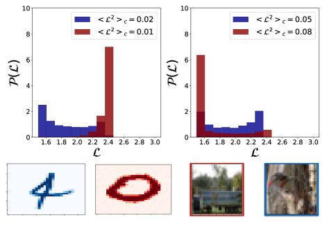
(a) The Monte Carlo loss distribution for two data sets studied.
Each distribution is color coded to their image.

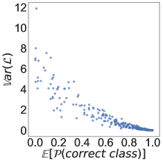
(b) Our “ground truth” uncertainty, the loss variance and average probability correlation function

Figure 1: Monte Carlo results for uncertainty

Before describing our uncertainty measure in detail, it’s worthwhile to obtain an understanding of the intrinsic or ground truth uncertainty that a model possess. To gauge the basic uncertainty measure, we constructed a “ground truth” measure of the uncertentity. This was done by training an ensemble of $4000$ LeNET networks with different initializations of the weights. For each ensemble we performed a classification of test portion in the dataset, and took the probability outcome from the softmax cross-entropy for correct class.

Fig. 1b shows the scatter plot between the variance in the loss, the uncertainty $\mathbb{{V}}ar[\mathcal{L}]$ and the average over the different probabilities of the correct label $\mathbb{E}[P\left(\text{correct label}\right)$. It is interesting to note that the point at which the probability of the model returning the correct label equals 1 corresponds to a transition point between the uncertainty and the probability being correlated and uncorrelated. Furthermore, there is a region where for a high uncertainty we have an ambiguous or almost random probability of the model returning the correct prediction.

4.3 Estimating the Uncertainty using LoVME

We next estimate the uncertainty using the variance $\mathbb{{V}}ar[N]$ and $\mathbb{{V}}ar[\mathcal{L}]$. In Fig. 1a we show two distributions of $\mathcal{L}$ and their respective test examples for the CIFAR10 and MNIST dataset. The MNIST data set quantitatively showed lower values of variance. This is to be expected as the network learns and converges within a few epochs to $99.7\%$ accuracy. Nonetheless, by plotting the distribution and calculating its variance, we can see the variance and uncertainty of each sample. Each color in Fig. 1a coincides with its distribution function, and the figure legend shows the variance values. For the CIFAR data set, there is a more distinct difference in the uncertainty values and in the spread of the distribution. It is also informative to look at the structure of a few chosen examples and their distributions, as shown in Fig. 1b shows the structure of a few chosen examples and their distributions. Surprisingly, most distributions either look bimodal or non-symmetric, which suggests that while the variance measures the uncertainty, higher moments might also come into play while considering a sample’s uncertainty. Our LoVME method demonstrates this important fact by evaluating the distribution explicitly, as well as by looking at higher moments.

4.4 Uncertainty in a Decision Metric

Estimating the uncertainty during the test stage also enables us to incorporate uncertainty into the decision metric. To show the effect of uncertainty on the prediction, we show the loss variance scores through both Receiver Operating Characteristic (ROC) and Area Under the Curve (AUC) plots.

For a probability score $P$ of a sample, we use its associated uncertainty as a binary confidence interval. Looking at $P\pm\mathbb{V}ar\left[\mathcal{L}^{2}\right]$ could either shift the sample into a TPR or a FPR, allowing us to use a type of confidence interval on top of the ROC, as shown in Fig. 2.Generating the confidence interval of the score allows us to set a certain threshold, above which a sample is too ambiguous to be classified as either a false positive or true negative. Thus, it can be eliminated from the ROC decision process. In Fig. 3 we show that removing high uncertainty examples increases the AUC when using our LoVME method, Monte Carlo dropout, and when calculating the naïve ground truth. Table 1 shows the different values of the AUC for each of the three methods.

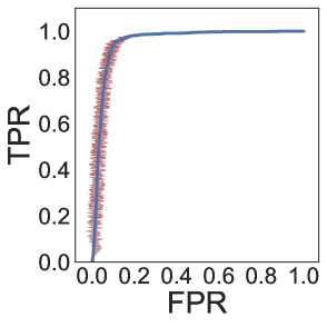
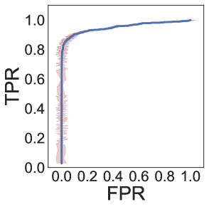
Figure 2: ROC for two classes, one of each dataset, with our “confidence intervals” measures

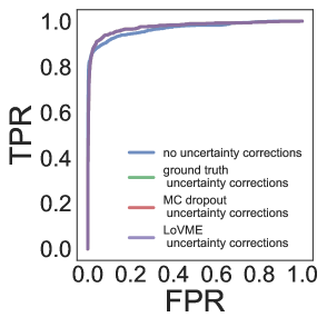
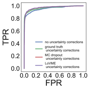
Figure 3: ROC curves with improvements based on uncertainty measures

	no uncertainty corrections	ground truth uncertainty corrections	MC dropout uncertainty corrections	LoVME uncertainty corrections
MNIST AUC	0.967	0.974	0.974	0.974
CIFAR10 AUC	0.956	0.967	0.972	0.973

Table 1: AUC values for the set of experiments

References

- [1] M Baity-Jesi, L Sagun, M Geiger, S Spigler, G Ben Arous, C Cammarota, Y LeCun, M Wyart, and G Biroli. Comparing dynamics: Deep neural networks versus glassy systems. arXiv preprint arXiv:1803.06969, 2018.
- [2] Riccardo Bellazzi and Blaz Zupan. Predictive data mining in clinical medicine: current issues and guidelines. International journal of medical informatics, 77(2):81–97, 2008.
- [3] Youngmin Cho and Lawrence K Saul. Kernel methods for deep learning. In Advances in neural information processing systems, pages 342–350, 2009.
- [4] Anna Choromanska, Mikael Henaff, Michael Mathieu, Gérard Ben Arous, and Yann LeCun. The loss surfaces of multilayer networks. In Artificial Intelligence and Statistics, pages 192–204, 2015.
- [5] Charles W Fox and Stephen J Roberts. A tutorial on variational bayesian inference. Artificial intelligence review, 38(2):85–95, 2012.
- [6] Yarin Gal. Uncertainty in deep learning. University of Cambridge, 2016.
- [7] Yarin Gal and Zoubin Ghahramani. Dropout as a bayesian approximation: Representing model uncertainty in deep learning. In international conference on machine learning, pages 1050–1059, 2016.
- [8] James A Hanley and Barbara J McNeil. The meaning and use of the area under a receiver operating characteristic (roc) curve. Radiology, 143(1):29–36, 1982.
- [9] Edwin T Jaynes. Information theory and statistical mechanics. Physical review, 106(4):620, 1957.
- [10] Mehran Kardar. Statistical physics of fields. Cambridge University Press, 2007.
- [11] Alex Kendall, Vijay Badrinarayanan, and Roberto Cipolla. Bayesian segnet: Model uncertainty in deep convolutional encoder-decoder architectures for scene understanding. arXiv preprint arXiv:1511.02680, 2015.
- [12] Alex Kendall and Yarin Gal. What uncertainties do we need in bayesian deep learning for computer vision? In Advances in Neural Information Processing Systems, pages 5580–5590, 2017.
- [13] Alex Krizhevsky and Geoffrey Hinton. Learning multiple layers of features from tiny images. 2009.
- [14] Yann LeCun. The mnist database of handwritten digits. http://yann. lecun. com/exdb/mnist/, 1998.
- [15] Yann LeCun, Yoshua Bengio, and Geoffrey Hinton. Deep learning. nature, 521(7553):436, 2015.
- [16] Yann LeCun, Bernhard E Boser, John S Denker, Donnie Henderson, Richard E Howard, Wayne E Hubbard, and Lawrence D Jackel. Handwritten digit recognition with a back-propagation network. In Advances in neural information processing systems, pages 396–404, 1990.
- [17] Yann LeCun, Léon Bottou, Yoshua Bengio, and Patrick Haffner. Gradient-based learning applied to document recognition. Proceedings of the IEEE, 86(11):2278–2324, 1998.
- [18] Paulo J Lisboa and Azzam FG Taktak. The use of artificial neural networks in decision support in cancer: a systematic review. Neural networks, 19(4):408–415, 2006.
- [19] David JC MacKay and Radford M Neal. Near shannon limit performance of low density parity check codes. Electronics letters, 32(18):1645, 1996.
- [20] Adam Paszke, Sam Gross, Soumith Chintala, Gregory Chanan, Edward Yang, Zachary DeVito, Zeming Lin, Alban Desmaison, Luca Antiga, and Adam Lerer. Automatic differentiation in pytorch. 2017.
- [21] Samuel S Schoenholz, Jeffrey Pennington, and Jascha Sohl-Dickstein. A correspondence between random neural networks and statistical field theory. arXiv preprint arXiv:1710.06570, 2017.
- [22] Nitish Srivastava, Geoffrey Hinton, Alex Krizhevsky, Ilya Sutskever, and Ruslan Salakhutdinov. Dropout: A simple way to prevent neural networks from overfitting. The Journal of Machine Learning Research, 15(1):1929–1958, 2014.
- [23] Han Xiao, Kashif Rasul, and Roland Vollgraf. Fashion-mnist: a novel image dataset for benchmarking machine learning algorithms, 2017.