Unwind: Interactive Fish Straightening

Abstract

The ScanAllFish project is a large-scale effort to scan all the world’s 33,100 known species of fishes. It has already generated thousands of volumetric CT scans of fish species which are available on open access platforms such as the Open Science Framework. To achieve a scanning rate required for a project of this magnitude, many specimens are grouped together into a single tube and scanned all at once. The resulting data contain many fish which are often bent and twisted to fit into the scanner. Our system, Unwind, is a novel interactive visualization and processing tool which extracts, unbends, and untwists volumetric images of fish with minimal user interaction. Our approach enables scientists to interactively unwarp these volumes to remove the undesired torque and bending using a piecewise-linear skeleton extracted by averaging isosurfaces of a harmonic function connecting the head and tail of each fish. The result is a volumetric dataset of a individual, straight fish in a canonical pose defined by the marine biologist expert user. We have developed Unwind in collaboration with a team of marine biologists: Our system has been deployed in their labs, and is presently being used for dataset construction, biomechanical analysis, and the generation of figures for scientific publication.

0 Research Application Francis Williams is with New York University. E-mail: francis.williams@nyu.edu. Alexander Bock is with New York University, the University of Utah, and Linköping University. E-mail: alexander.bock@liu.se. Harish Doraiswamy is with New York University. E-mail: harishd@nyu.edu. Cassandra Donatelli is with Tufts University. E-mail: cassandra.donatelli@tufts.edu. Adam Summers is with the University of Washington. E-mail: fishguy@uw.edu. Daniele Panozzo is with New York University. E-mail: panozzo@nyu.edu. Cláudio Silva is with New York University. E-mail: csilva@nyu.edu. Our system, Unwind, accepts CT scans of one or more fishes which are bent or twisted as input (top-left). By selecting two endpoints at the extrema of a single fish skeleton, a user can quickly and interactively remove any torque and bending from the input scans (top-right). Finally our system outputs a high resolution volume of the straightened fishes in a canonical pose as well as provenance data for the deformation (bottom).

1 Introduction

New tools often lead to scientific discoveries, and this is particularly true for new 3D imaging technology, which has helped advance many scientific areas. The availability of 3D imaging scanners has resulted in tens of thousands of large datasets to be analyzed. Our work is centered on the ScanAllFish and oVert projects, which are large-scale efforts to (CT) scan all the world’s known species of fishes and other vertebrates [scan-all-fish-science, Watkins2018]. The Micro-CT scan allows scientists to determine the skeletal structure of a variety of fishes, opening the doors to a better understanding of relationships among skeletal elements and the degree of skeletal mineralization, as well as enabling population-wide studies that were previously impossible. Both volumetric and surface renderings are useful for making quantitative measures of skeletal parameters that are used to build evolutionary trees and demonstrate the directional variation of morphology over evolutionary time [Hall2018, Kolmann2018, Stocker2019].

The extracted skeletal geometry can be used to make physical models of function and support the understanding of swimming motions by combining finite element modeling and computational fluid dynamics. Finally, scans allow researchers, curators, and scientific communicators to make 3D printed replica of these fishes for expositions and museum archives. The huge number of fish, their variety, and the scanning techniques involved cause unique challenges. As previously described in Bock [Bock:2018], fishes are packed together for scanning purposes, with multiple fishes being placed inside a single scanning chamber. Every fish is twisted in a different way, they have different sizes and shapes, and those that are too long are curled up to fit into the scanner. This method of packing multiple fishes together allows for rapid scanning of multiple species, but causes difficulty in analyzing the raw volumes. In fact, there are two fundamental problems that hamper effective use of the data: (1) the difficulty of separating each fish into its own volume and (2) dealing with fishes that are bent and twisted in different poses, making side by side comparisons impossible.

While the first problem can be addressed using existing segmentation techniques [Bock:2018], the second problem is the challenge that we address in this paper: we propose an interactive pipeline to reverse this undesired deformation, restoring the original shape of the fish into a canonical straight pose, and thus facilitating the analysis and visualization of these valuable datasets.

Ideally, fish straightening would be performed completely automatically. Unfortunately, this requires the detection and measurement of the distortion that each exemplar underwent during the packing in the CT scanner. This information is impossible to acquire with a CT scan, since it requires the measurement of the volumetric stresses in the exemplar itself. Custom interactive tools therefore play an important role in helping users effectively guide this straightening process. While existing off-the-shelf software support deforming 3D volumes, these approaches require users to work directly in 3D making its usage time consuming even for experienced users, let alone our target users who are not familiar with 3D modelling software. Hence, it is essential to optimize user interactions so as to not overburden the users in their workflow. In fact, minimizing human effort for various tasks has recently gained traction in the design of user interfaces. For example, Hong et al. [Hong2014] showed that designing an interface with minimal user-selectable information was most effective in the context of understanding accessibility in cartographic visualization; Ono et al. [Ono2019] designed an interface to track baseball plays that reduces the annotation burden on the user. Similarly, Choi et al [Choi2019] proposed an approach that automatically emphasizes words within a document and prividing recommendations in order to reduce the burden on users labeling documents.

Following along the above strategy, we design Unwind, a user-driven, interactive volumetric straightening system that provides a single interface to start working directly with the original CT data, and enables the marine biologist to quickly and efficiently process the twisted volumes into clean data in a canonical straight pose. The user interaction is divided in two phases: (1) a selection phase, where the user picks a pair of 3D points to identify the extrema of the spine of a fish, from which the system automatically extracts a skeleton and an initial approximation of the straightened fish; and (2) a refinement (or tuning) phase, where the user navigates the 2D cross-section of the fish and fine-tunes the deformation by specifying additional rotations required to eliminate the torque and bending in the fish. The system is based on a simple but novel deformation method which is specifically designed for undoing the bent and twist introduced during the packing of multiple fishes, and that can be efficiently implemented on a GPU to ensure an interactive volumetric rendering of the undeformed dataset. Unwind is already in use in the labs participating in the ScanAllFish project.

The contributions of this paper can be summarized as follows:

• The design of an interactive tool allowing users to process a CT image, extracting individual fishes, and straightening them. This tool allows a marine biologist to process a dataset in 6 minutes on average.

• A simple deformation algorithm that enables an intuitive and easy user interaction by allowing users to interact with 2D slices instead of the complete 3D volume.

• A preliminary user evaluation, comparing the time and quality obtained by 10 users processing a representative dataset.

• A demonstration of the effectiveness of Unwind through expert feedback on processing 18 fishes.

• A reference system implementation.

2 Related Work

Our approach combines techniques from geometry processing, to estimate the initial deformation, with rendering and deformations techniques developed within the visualization community. Here, we give an overview of the most closely related works, and we refer to [PMP:2010, Johnson:2004:VH:993936] for a complete overview.

Skeletonization via Discrete Maps.

We review here the skeletonization works applicable in our setting, and we refer an interested reader to [Tagliasacchi:2016] for a detailed overview.

Our skeleton construction is based on a harmonic volumetric parametrization [Wang:2004:harmonic, Li:2007:Harmonic] constructed from a pair of user-provided landmarks. The isosurfaces of the scalar function are averaged to find points in the center of the fish: this construction is inspired by the hexahedral method proposed in [gao2016structured] and the tubolar parametrization proposed in [Livesu:2017].

It is important to observe that the parametrization induced by these functions is not bijective [Schneider:2015], and it is thus not a proper foliation [Campen:2016]: however, this is not a problem in our case since we use it only to compute an approximate skeleton. We opted for this skeleton extraction procedure since it allows users to intuitively and interactively control the skeleton, which is mandatory to make our system able to process challenging datasets. For a complete overview of skeletonization techniques, we refer an interested reader to [Tagliasacchi:2016].

Volumetric Deformation.

This problem has been heavily studied in both in the context of (1) volumetric parametrization, where a energy minimizing, quasi-static solution is found via numerical optimization, (2) in physical simulation, where the focus is on modeling dynamics effects, and (3) in space warping techniques, where a explicit reparametrization of the space is used to warp an object. Since we are not interested in dynamics (we only need to deform the volume once), we only review the parametrization and free form deformation literature, and we refer an interested reader to [Witkins:1997, Meier:2005, Nealen:2006, Sifakis:2012, skinningcourse:2014] for an overview of dynamic physical deformation techniques.

Volumetric Parametrization.

A convex approximation of the space of bounded distortion (and thus inversion-free) maps has been proposed in [Lipman:2012, Kovalsky:2015], allowing to efficiently generate these maps both in 2 and 3 dimensions. These methods do not require a starting point, but they might fail to find a valid solution in challenging cases. A different approach, guaranteed to work but requiring a valid map has been proposed in [Hormann:2000, Degener:2003]: the idea is to evolve the initial map to minimize a desired cost function, while never leaving the valid space of locally injective maps. Many variants of this construction have been proposed, either enriching existing deformation energies with a barrier function [Schuller:2013], or directly minimizing energies that diverge when elements degenerate [Smith:2015]. Specific numerical methods to minimize these energies have been proposed, including coordinate descent [Hormann:2000, Fu:2015], quasi-newton approaches [Smith:2015, Kovalsky:2016, Rabinovich:2017, Shtengel:2017, Claici:2017], and Newton [Schuller:2013] methods. A last category of methods [Fu:2016, Poranne:2017] produces an initial guess separating all triangles and rotating them into the UV space, and then stitches them together using Newton descent. However, all these methods are computationally intensive, and not suitable for interactively deforming high-resolution CT scans.

Space Warping.

Closed-form volumetric deformations have been defined using lattices [Sederberg:1986, Barr:1984, Coquillart:1990] or other parametrizations [Chen:2003]. While not directly minimizing for geometric distortion, they have the major advantage of being directly usable in a volumetric rendering pipeline, enabling to render in real-time the deformed volume. Our approach is also directly usable in a real-time volumetric rendering pipeline and uses a keyframed skeletal parametrization to define the deformation.

Volume wires [Volume_Wires] uses a skeleton to define a free form deformation, parametrizing it with values attached to the skeleton itself. Volume wires relies on a computationally intensive evaluation which prevents its use in a real-time rendering systems. Our method shares the idea of using a skeleton to parametrize the deformation, while providing detailed deformation control using keyframes, an algorithm to automatically estimates an initial deformation, and being specifically tailored to be used in an interactive volumetric rendering system.

Interactive Applications.

Many variants of the previous volumetric deformation techniques have been used in interactive applications in the visualization community: since a complete overview is beyond the scope of this work, we limit our review to the most closely related works, and we refer an interested reader to the surveys by Sun et al [sun2013survey] for visual analytics, and Liu et al. [liu2014survey] for information visualization techniques.

Closely related to this work, Correa et al. [correa2007volume] introduced an interactive visual approach to deform images as well as volumetric data based on a set of user-defined control points. Here, the deformation is controlled based on the movement of these control points. Even though their formulation introduced distortions in other regions of the data, since their focus was on illustrative applications and volume exploration and visualization, such distortions were acceptable since they were occluded in the visualization. On the other hand, our goal is to generate data that will be further analyzed by the marine biologists. It is therefore necessary that such distortions are avoided. Such distortions are common in other approaches as well that perform volume deformation with the focus on exploration and/or animations [correa2007illustrative, Kwon:2018].

There have also been visual approaches that target generating illustrations with the focus on medical data [MRH08, Li:2007], in particular, generating views when the covering surface is “cut open”. Since these approaches distort the data that is deformed, they are not suitable for our work. Nakao et al. [Nakao:2010, Nakao:2014] proposed an interactive volume deformation, also catered towards medical applications, which deforms the volume based on a proxy geometry that approximated the volume. However, the proxy geometry itself is computed in a preprocessing phase, which makes the combined pipeline not interactive.

Directly related to CT scans of fishes, in our previous work we proposed TopoAngler [Bock:2018] that combines a topology based approach with a visual framework to help users segment fishes from the CT data. TopoAngler is used as a preprocessing step in this work, to extract a segmented fish (Section 5).

3 Unwind: Design Overview

Processing one CT dataset containing a packed set of fishes requires multiple steps, which are currently only possible by using different software packages, and that require conversions and manual processing to be combined: (1) to process the scanned images into a 3D volume format (and optionally subsample the volume), (2) to segment and export individual fishes from the 3D volume, and (3) to deform the fishes into a canonical pose. While straightening the individual fishes is desirable, given that there exists no off-the-shelf tool to accomplish this, it was not possible for the users to do this. Our goal in the design of Unwind is to provide a single, efficient, and intuitive tool to process the CT data once they obtain it from the scanning software, enabling non-expert users to process the massive amount of data which is acquired daily in marine biology labs. To accomplish this, we divide the entire process into four stages:

1. Load CT data: The user can directly load the output from the CT scanner, which is then subsampled to fit in the video memory of the workstation to ensure an interactive preview of the deformation.

2. Segment and extract a single fish: For the initial segmentation, we decided to integrate the functionality from the open sourced TopoAngler [Bock:2018] due to three reasons: (1) it is widely used by marine biologists, being the only tool specifically designed for this tasks; (2) the user interaction is intuitive, requiring only a single parameter accompanied with a few clicks from the user to select the required subvolumes and, (3) it is interactive, providing a live preview even on complex volume scans of multiple fish. This segmentation approach first generates a hierarchical segmentation based on the join tree of the input data [CSA03], and then allows the user to interactively choose the simplification to be performed and select the segmented sub-volumes corresponding to the fish. We refer the reader to [Bock:2018] for a detailed description of this algorithm.

3. Estimate the straightened volume: In this stage, our goal is to semi-automatically estimate the straightened volume using user input. Since the spine (or the mathematical skeleton) of the fish traces out a curve in space, it was a natural decision to define our deformation as a warping of a curve in space. This requires to compute the spine geometry followed by defining the deformation based on the warping that straightens it. While automatically extracting the spine for a given fish would be ideal, existing skeletonization methods are not easily adaptable in our setting given the varied shapes and sizes different fishes take. Therefore, we decided to employ a minimalistic user assisted approach, wherein we require the user to select the two extremal end points of the fish, which are then used to find the fish skeleton. Note that the alternative of allowing the user to manually specify the 3D curve corresponding to the spine is an arduous task requiring the interaction with a 3D volume.

4. Refine the straightening. Since our deformation occurs along a curve in space, it was very natural to allow the user to interact with 2D cross sections along that curve. Once the approximate spine is computed, we define a set of coordinate frames along this curve, which is then used by the user to refine the deformation. This process mainly involves the user aligning the coordinate frames to generate an accurate spine from the estimated curve. Using such an interface was inspired by popular video editing software in which users can edit a set of keyframes. The simplicity of editing in 2D combined with real time 3D visualization of the deformation makes for an easy-to-use tool allowing extremely precise control over the deformation. Not only is this deformation transformation simple mathematically (thus allowing interactivity), but users could also easily understand this procedure simply by using the software without requiring a mathematical explanation.

The next two sections focuses on the third and fourth steps of the above workflow, and describes in detail the user interface of Unwind. We would like to note that the described system was designed over multiple iterations spanning over a year based on constant feedback from our collaborators (who were also the initial users). We discuss this process after the description of the user interface.

4 Cylindrical Deformation

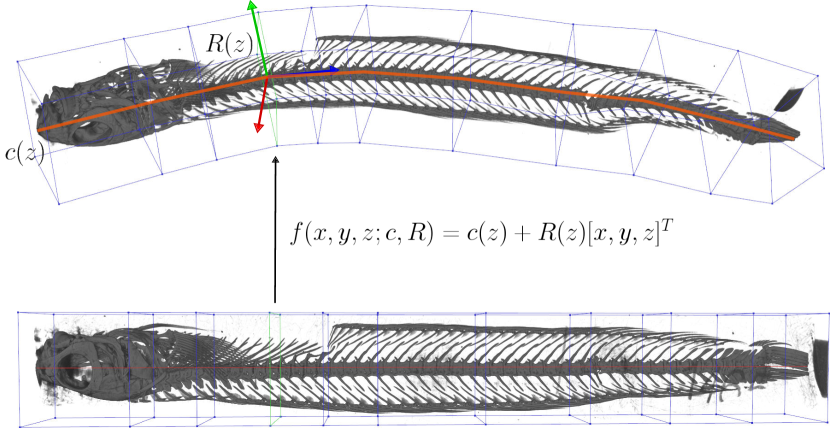
Figure 1: An illustration of our volumetric deformation: The density at a point $(x,y,z)$ in the straight volume is determined by the cross sectional plane $R(z)$ centered at $c(z)$, where $c(z)$ is a piecewise linear curve sweeping the spine of the fish and $R(z)$ is a frame centered at $c(z)$ defining the orientation of the fish at a given position. $R(z)$ and $c(z)$ are specified at a set of keyframes (the blue squares) and interpolated linearly in between.

Without loss of generality, we assume that fishes are straightened one at a time. If more than one fish is present in the scanned volume, we isolate individual fishes using TopoAngler [Bock:2018]. The key idea in our approach is to identify a deformation function $f$, which transforms an axis aligned bounding box (which will contain the straight fish), into a deformed version of the fish. This function, being the inverse of the deformation that the fish underwent, will be then used to recover the straight fish.

More concretely, we are interested in a mapping, $f$, which deforms a straight cylindrical region $V_{\text{straight}}$ into a deformed one $V_{\text{twist}}$ such that the central axis of the $V_{\text{straight}}$ is mapped to a curve $c(t)$, which is aligned with the body of the twisted fish. Furthermore, for every $z$ coordinate in $V_{\text{straight}}$, we define a rotation matrix $R(z)$ which maps points off the central axis to points in $V_{\text{twist}}$. The set of rotation matrices $R$ captures both the “bends” that the fish underwent as well as the “twists” (or torsion) in the fish. Figure 1 illustrates one such deformation function $f$.

Thus, to parameterize $f$, we require a space curve $c(t)=\begin{bmatrix}c_{x}(t),c_{y}(t),c_{z}(t)\end{bmatrix}^{T}$ and a continuous field of rotation matrices $R(t)=\begin{bmatrix}u(t)^{T},v(t)^{T},n(t)^{T}\end{bmatrix}^{T}\in SO^{3}$, allowing us to write:

$$f(x,y,z;c,R)=c(z)+x\cdot u(z)+y\cdot v(z)$$ (1)

Intuitively, the direction along $n$ in $R$ points along the skeleton (central axis) of the fish, while the $u$ and $v$ directions define the right and up directions of the fish respectively. Thus, $n$ allows us to undo any bending in the fish while $u$ and $v$ allow us to remove torsion.

In our setting, we use an arclength parameterized piecewise linear curve for $c(t)$. Note that the arclength parametrization ensures that the mapping will be close to an isometry independently on the speed of the parametrization of $c$. This is important since it allows the user to freely change the parametrization speed by adding additional keyframes, without introducing unwanted distortion (Section 5). Specifically, $c(t)$ can be parameterized by vertices $e_{1},\ldots e_{m}\in\mathbb{R}^{3}$. Letting $d(e_{i})=\sum_{j<i}||e_{j+1}-e_{j}||_{2}$, we can write $c(t)$ explicitly as:

$$c(t)=\lambda(t)e_{k(t)}+(1-\lambda(t))e_{k(t)+1}$$ (2)

where

$$k(t)=\operatorname*{arg\,min}_{i,(d(e_{i})<t)}(t-d(e_{i}))$$ (3)

$$\lambda(t)=\frac{t}{e_{k(t)}-d(e_{k(t)+1})}$$ (4)

To define $R(t)$, we define orthonormal coordinate frames $R_{1}=(u_{1},v_{1},n_{1})^{T},\ldots,R_{m}=(u_{m},v_{m},n_{m})^{T}\in SO^{3}$ at each vertex $e_{i}$ of $c$. For $R(t)$ to be continuously defined at all points along $c$, we identify the unit normals, $n_{i}$, with points on a sphere and spherically interpolate the $n$ directions between adjacent $R_{i},R_{i+1}$:

$$R(t)=\text{SLERP}(n_{k(t)},n_{k(t)+1},\lambda(t))R_{k(t)}$$ (5)

As we show next, the parameters of the deformation function $f$ are initially estimated by our system, and optionally interactively refined by the user in a second stage to compute the final straightened fish.

5 Interactive Fish Straightening

Unwind uses the cylindrical deformation (Equation 1) to assist users in straightening deformed fishes. Once the individual fish is isolated from the input CT data, the remaining stages of the process can be further divided into the following 4 steps:

1. Compute the harmonic function used for estimating the deformation function $f$.

2. Estimate the parameters of the deformation function $f$.

3. (Optional) Refine the parameters of the deformation function $f$.

4. Export the straightened fish.

We now describe in detail each of these steps and the associated visual interface of our system. Each step comprises of its own set of visualization widgets, and the user can move forward and back between the different steps. The entire workflow is illustrated in the accompanying video. Note that the user input is used to guide this process during the different steps.

5.1 Compute Harmonic Function

We first approximate the fish by a smooth curve in order to estimate the parameters of the deformation function $f$. This curve is computed as the set of centroids of level sets of an harmonic scalar field defined on the volume, following a technique similar to [gao2016structured].

Discretization.

Different techniques could be used to compute the harmonic function, and we opted for a finite element method due to its efficiency, simplicity, and robustness. While it is possible to use directly the voxel grid as a space discretization, this would be prohibitively expensive on the high resolution CT scan. Downsampling the image is a possibility, but it would lose the high-frequency details and risk to lead to disconnected components in the thin regions of the fish. We therefore opt for an adaptive tetrahedral mesh, generated using an implementation of Isosurface Stuffing [labelle2007isosurface], which strikes a good balance between boundary approximation and computational efficiency. While unlikely, it is possible that the generated tetrahedral mesh is made of multiple disconnected components, either due to lack of resolution, or due to the TopoAngler segmentation. To ensure there is only a single connected component, we inflate the voxel grid until all the connected components are merged using [Chen:2018].

User-Provided Extrema.

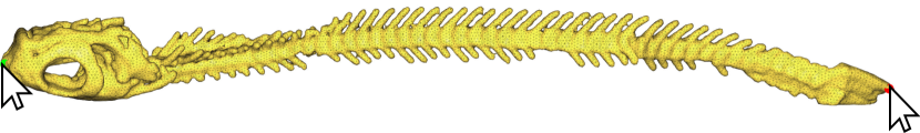
Figure 2: The user selects two extrema on the endpoints of the fish by clicking on the extracted tetrahedral mesh.

The extrema of the harmonic function, used as boundary conditions, are provide by the user with an end-point selection widget allowing the user to select points on the segmented fish (see Figure 2). These points corresponds to the head and tail of the fish, making it straightforward for the user do this selection.

The two endpoints are then used to compute a discrete harmonic function with Dirichlet boundary conditions setting the head vertex $v_{\text{head}}$ and the tail vertex $v_{\text{tail}}$ as a source and sink:

$$(Lu)_{i}=\begin{cases}0&\text{if }u_{i}\neq v_{\text{head}},u\neq v_{\text{tail}}\\ 1&\text{if }u_{i}=v_{\text{head}}\\ -1&\text{if }u_{i}=v_{\text{tail}}\end{cases}$$ (6)

Here, $L$ is the discrete Laplace-Beltrami Operator [PMP:2010], and $u$ is a scalar field defined at each vertex of the tetrahedral mesh. While solutions to Equation 6 produce fields whose level sets trace out a reasonable skeleton approximation, the spacing between level sets is not uniform. To remedy this issue, we resample the curve using a fixed spacing between vertices in ambient space. To ensure the resampling process does not discard details, we use a sampling width which is half the size of the smallest segment in the curve traced out by the level sets of the harmonic solution.

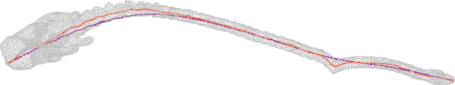
Figure 3: Estimated skeletons using the centroids of level sets: The red curve shows the piece-wise linear curve where the vertices are 100 centroids of the level sets uniformly sampled on the scalar function $u$ (Equation 6 defined on the tetrahedral mesh. The purple curve is the result of applying 50 smoothing steps the red curve.

5.2 Estimating Parameters $c(t)$ and $R(t)$

To generate an initial estimate for the piecewise linear curve, $c(t)$, we sample $k$ level sets of $v$ at isovalues uniformly spread on $[-1,1]$. We then compute the centroids, $c_{1},\ldots,c_{k}\in\mathbb{R}^{3}$, of these level sets. While the piecewise linear curve whose vertices are the $c_{i}$’s traces a curve approximating the bend of the fish, the curve itself might be noisy due to the complex boundary geometry. We thus apply $s$ iterations of Laplacian smoothing (replacing every vertex with the average of its 2 neighbours) to smooth the curve. Figure 3 compares two curves before and after smoothing. Specifically, if $c_{i-1},c_{i},$ and $c_{i+1}$ are consecutive vertices of the curve, one iteration of smoothing can be written as:

$$\text{SMOOTH}(c_{i})=c_{i}^{\prime}=\frac{c_{i-1}+c_{i+1}}{2}$$ (7)

Once we have vertices $c_{i}^{\prime}$, we then compute orthogonal coordinate frames $R^{\prime}_{1},\ldots R^{\prime}_{k}$, where $R_{i}^{\prime}=(u_{i}^{\prime},v_{i}^{\prime},n_{i}^{\prime})^{T}\in\mathbb{R}^{3\times 3}$. First we compute $n_{i}^{\prime}$ at each of the $c_{i}^{\prime}$ using central differences on the interior and one sided differences at the boundary:

$$n_{i}^{\prime}=\begin{cases}\frac{c^{\prime}_{i+1}-c^{\prime}_{i+1}}{||c^{\prime}_{i+1}-c^{\prime}_{i+1}||_{2}}&\text{if }1<i<k\\ \frac{c^{\prime}_{i+1}-c^{\prime}_{i+1}}{||c^{\prime}_{i+2}-c^{\prime}_{i}||_{2}}&\text{if }i=1\\ \frac{c^{\prime}_{i+1}-c^{\prime}_{i+1}}{||c^{\prime}_{i}-c^{\prime}_{i-2}||_{2}}&\text{if }i=k\end{cases}$$ (8)

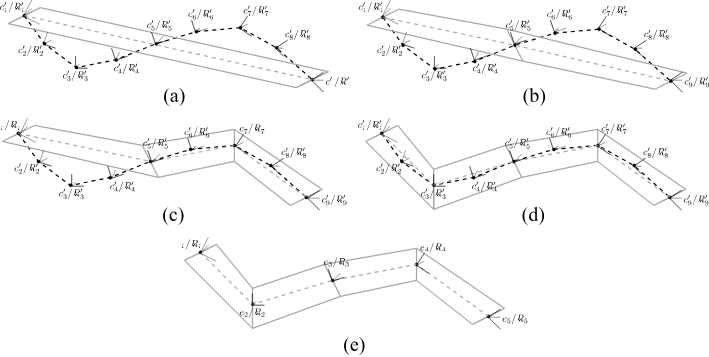
Figure 4: Computing a minimal set of parameters by subdivision: The black dotted line illustrates the initial estimated parameters $c_{i}^{\prime}$ and $R_{i}^{\prime}$, using the method described in Section 5.2. We compute the gray prism by connecting two squares on the $u_{1}^{\prime}-v_{1}\prime$ and $u_{9}^{\prime}-v_{9}^{\prime}$ planes. We progressively subdivide the prism at vertices $c_{i}^{\prime}$ until the subdivided prisms fully contains all the $c_{i}^{\prime}$. This refinement procedure yields a new, reduced set of parameters $e_{1},\ldots e_{5}$ and $R_{1},\ldots,R_{5}$.

We then compute $u_{i}^{\prime}$ and $v_{i}^{\prime}$ by projecting the $x$ and $y$ axes into the plane defined by $n_{i}^{\prime}$. If such a projection degenerates, we repeat this procedure with the $x$ and $z$ axes as well as the $y$ and $z$ axes (one of them has to succeed since the skeleton is not degenerate by construction):

$$u_{i}^{\prime}=\hat{x}-\hat{x}^{T}n_{i}*n_{i},$$ (9)

$$v_{i}^{\prime}=\hat{y}-\hat{y}^{T}n_{i}*n_{i}.$$ (10)

The result is a piecewise linear curve with vertices $c_{1}^{\prime},\ldots c_{k}^{\prime}$ and orthonormal bases $R_{1}^{\prime},\ldots R_{k}^{\prime}$ at each vertex. Note that the number of level set samples, $k$, and smoothing iterations, $s$ are user-tunable parameters. The default is $k=100$ and $s=50$ and our users did not change them in any of their experiments.

Computing a Minimal Set of Parameters.

Having a large numbers of parameters can become cumbersome to a user when refining the deformation (see Section 5.3 below). Thus, while we could use the parameters $c_{1}^{\prime},\ldots c_{k}^{\prime}$ and $R_{1}^{\prime},\ldots R_{k}^{\prime}$ for the deformation, we opt instead to compute a minimal set of parameters $e_{1},\ldots,e_{m}$ and $R_{1},\ldots R_{m}$, $R_{i}=(u_{i},v_{i},n_{i})^{T}$, which agree with the $c_{i}^{\prime}$’s and $R_{i}^{\prime}$’s.

To compute these new parameters, we select a radius $r$ and construct a prism whose bases are squares with side lengths $2r$. Each base is centered at $c_{1}^{\prime}$ and $c_{k}^{\prime}$ and is oriented to lie in the planes $n_{1}^{\prime}$ and $n_{k}^{\prime}$ with the sides aligned with $u_{1}^{\prime}$, $v_{1}^{\prime}$ and $u_{k}^{\prime}$, $v_{k}^{\prime}$. Figure 4(a) shows a 2D illustration of the initial configuration for an example curve.

Then, while the prism does not fully contain the vertices, $c_{1}^{\prime},\ldots c_{k}^{\prime}$, we subdivide it by first choosing a vertex $c_{\text{mid}}^{\prime}$ and frame $R_{\text{mid}}^{\prime}$, and then splitting a prism into two with a base centered at $c_{\text{mid}}^{\prime}$ and aligned with $R_{\text{mid}}^{\prime}$. Figure 4(b)–(e) illustrates this subdivision procedure.

The resulting $e_{i}$ and $R_{i}$ are the vertices and coordinate frames of the subdivision location used to construct the prism. The radius hyperparameter, $r$ is user selectable: A larger radius will yield a coarser approximation, and a smaller radius will yield a finer one. By default we set $r$ to 10 voxel-widths, and our users did not adjust it in any of their experiments.

Figure 5 shows an example of the initial estimated deformation on a fish scan.

Figure 5: The deformation automatically estimated from the input (top) captures the majority of the distortion (middle) and can be further refined adding additional keyframes (bottom).

Handling Disconnected Components.

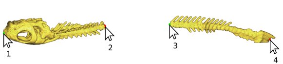
Figure 6: In cases where the segmentation outputs disconnected components, we recover a curve approximating the skeleton by selecting endpoints on each connected component. In the figure, the user selects points 1, 2, 3, and 4 and the system estimates a curve between 1 and 2 and another between 3 and 4 which are joined by a line connecting 2 and 3.

There are cases where the components corresponding to a fish are significantly far apart that the dilation operation performed when identifying the sub-volume corresponding to the fish is not sufficient to merge the two components (see Section LABEL:sec:feedback for details). To handle such a scenario, we allow the user to select the end points of the different components in order, compute the harmonic function and estimate the deformation function parameters for each component, and use the ordered end points to merge the different curves into a single one (Figure 6).

5.3 Deformation Refinement

We allow the user to interactively edit and refine the deformation parameters. The user interface for this step comprises 3 widgets (Figure 7): a 2D view for editing in a cross section (Figure 7, left), a 3D view showing the effect of the edits in real time (Figure 7, right), and a control widget providing buttons and sliders to help the user perform the deformation (Figure 7, bottom).

Control Widget.

This widget provides the user with a slider (Figure 7, 1) that controls the parameter $t$ along the parametric curve $c(t)$. Users can use this to move along this curve to identify locations to edit the deformation. Buttons at either end of the slider allow the user to skip to parameters corresponding to the parameter vertices, $e_{i}$. The widget also provides options for the user to add new vertices, $e_{i}$ and frames, $R_{i}$, as well as delete existing vertices and key frames. Alternatively, any interaction in 2D view will automatically add a new vertex and key frame along the curve. Additionally, this widget enables the user to view and change the transfer function of the rendered volume and includes controls to recenter the camera and toggle between the straight and deformed views.

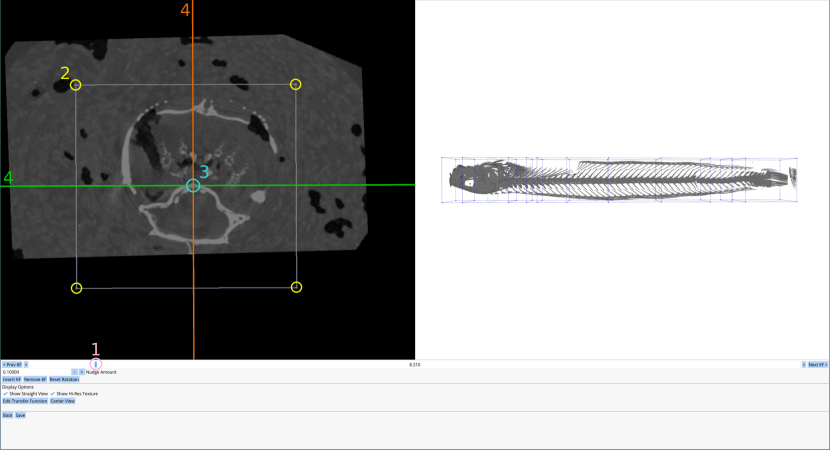
Figure 7: Our user interface for performing interactive deformations.

2D View.

This view shows a cross section of the volume in the plane orthogonal to $n(t)$ corresponding to the currently selected parameter $t$ in the control widget. Visual cues are overlaid over this cross section to allow user modify the different deformation parameters. These cues include:

1. A box corresponding to the region of space in the input which will be deformed to generate the output (Figure 7, 2). This represents the the prism base corresponding to the current parameter vertex $e_{i}$. The user can adjust the size of the bounding prism, $V_{\text{cage}}$, by dragging the corners of this box.

2. A point corresponding to the position of $c(t)$ in the 2D plane orthogonal to $n(t)$ (Figure 7, 3). Dragging this point allows the user to change change the position of vertices on the parametric curve.

3. The directions $u(t),v(t)$ in the 2D plane. The user can also rotate the $u(t)$ and $v(t)$ vectors around $n(t)$ by holding shift and dragging (Figure 7, 4). This feature allows the user to align $u(t)$ and $v(t)$ with the principal directions of the fish, thus allowing for the removal of any torsion which may be present in the twisted input.

3D View.

Depending on the option selected in the control widget, the 3D view visualizes in real time, either the straightened fish or the deformed bounding cage and curve $c(t)$. The former option allows the user to receive real-time feedback on how their edits affect the output, while the latter view allows the user to visualize how well their curve approximates the skeleton of the fish. The straightened volume is obtained by sampling the deformation function $f$ after each update to its parameters. This is accomplished by mapping a regular lattice (which is used for the volume rendering) to the input volume which is then sampled using trilinear interpolation. To provide real time feedback at interactive rates, we perform this sampling using the fragment shader as part of the rendering pipeline.

5.4 Real-Time Rendering and Export

Our system, similarly to existing volume deformation pipelines [Chen:2003], enables real-time rendering of the warped volume, allowing the user to instantaneously see the result of their actions. To render deformations in real time, our system computes a straight volume by evaluating $f(x,y,z)$ (Equation 1) along cross sections in $z$. We implement this evaluation in an OpenGL shader which renders cross sections along $z$ into a volume texture. The texture size is determined by the prisms described in Section 5.2.

Once the user is satisfied with modeled deformation, the straightened volume can be exported onto disk. We use the same procedure for exporting as we do for real time rendering. To preserve the correct dimensions during export, the depth ($z$-direction) of the volume is set to the arclength of the linear curve $c(z)$. The width and height ($x$ and $y$ directions) are set to maintain the same aspect ratio as the prisms. The user can optionally edit the size of the exported volume.

In addition to exporting the volume, our application allows the user to save a session to disk and reload it later for further editing or inspection. This feature is important to ensure provenance, enabling to store a direct mapping between the straightened fish and the original RAW volumetric dataset.

6 Design Process

Once the problem (straightening scans of fish) was identified, we examined example scans and analyzed the existing workflow used by the marine biologists for manipulating CT scans. While there are manual deformation systems built into several commercial programs (e.g., Amira, Aviso) which have been used in the past (e.g., straightening the deformed jaw of a megamouth shark [Dean2012]), these methods require users to manually place and adjust reference points in 3D to perform the necessary deformation. To quote one of our collaborator, when asked how effective these tools were for straightening CT scans, his response was: “I would say it simply cannot be done. A poor job took hours and hours over several days when I worked on the megamouth shark”.

Moreover, the gold standard for 3D data acquisition demands that a museum specimen be imaged. That means the shape of the fish is set by the fixative used when the specimen was collected. So, fish are always, whether scanned singly or in groups, scanned with bent spines. Manual, physical straightening of the fish before scanning is difficult, time consuming, and can lead to damage to the specimen, and it is thus not a viable option.

So, our next step was to consider the adaptability of existing free form deformation based approaches to perform the deformation. This requires users to manually deform a lattice bounding the fish directly in 3D. This was an onerous task even for an expert savvy with 3D modelling tools and it requires a high learning curve. We therefore decided to build a custom tool for this purpose with aim of making the straightening process easy for our target users. In particular, our goal was to design an interface that requires minimal and simple user interaction using metaphors that the users were already familiar with.

The first version of our tool used a skeletal-based deformation performed by setting the length of the spine and the number of skeleton vertices. Here the user selects two endpoints on a segmented mesh, inputs a number of skeleton vertices, and the software computed a deformation using a volumetric extension of ARAP [ARAP_modeling:2007] to map the automatically computed skeleton to a straightened mesh. While this approach had only a few user inputs, it often failed if the skeleton extraction was imperfect. It also required the segmented mesh to include minute details of the fish which could not be easily obtained through Topoangler.

So, in the next iteration, we tried using a cage based deformation that used the above estimated skeleton to derive the initial bounding cage. The user then had to manipulate cage vertices to get the deformation. Again, depending on the quality of the segmented mesh obtained from Topoangler, the initial cage would often be far from the desired cage and hence required several interactions from the user to rectify it. Moreover, manipulating individual skeleton vertices was not only cumbersome, taking a lot of user time, but it also involved a high learning curve especially for users not familiar with 3D modeling tools.

To overcome the problems caused by the coarse segmentation, we decided to use our curve-based approach, which requires computing only the main spine of the fish. After observing the current tools used by the biologists for segmentation, we noticed they were split into a 2D editing widget for selecting a boundary along a cross section and a 3D widget for selecting an axis aligned cross section along x, y or z axis. Given this familiarity, we decided to use a 2D cross section view as well to help users adjust the alignment of the estimated spine with the actual spine and used a 3D view to show the results of the adjustments in real time. This design also reduced the user interactions, and removed unnecessary input such as cage vertices. Furthermore, this design was also robust in the sense that even in rare cases when the skeleton estimation is far from the actual spine of the fish, the user can easily recover by fixing the spine vertices.

The above version of the tool was deployed at our collaborators’ labs during which time we were actively collecting feedback and fine tuning the system. In particular, as more people started using the tool for straightening different fish scans, certain important shortcomings were noticed that had to be fixed. In particular, (1) there were cases where the segmented fish consisted of disconnected segments, which had to be fixed (as described earlier); (2) the users requested the ability to rotate keyframes along a second axis (in the initial version one could only rotate about the normal tangent to the skeleton curve). This was necessary to correct minor warping that was sometimes caused in the output volume; and (3) Since the estimated skeleton tracks the spine, in some cases when the straightened volume was exported, fleshy parts of the bits near the endpoints of the spine were missing. To overcome this, an option was added to pad the exported volumes with additional keyframes at the endpoints.

7 Limitations and Concluding Remarks

We introduced a novel system for supporting the creation of a large encyclopedia of CT scans of fishes, providing a user-assisted procedure to undo the unwanted deformation introduced in the scanning process. We demonstrated the utility of our system, evaluating quantitatively the error introduced in baseline comparisons, and qualitatively over real-world scans. The system is available as open source, and it is in active use in our collaborator’s labs.

Limitations.

Our system has a high GPU memory requirement, which requires a high-end graphics workstation to run. Reducing this requirement is important to foster the applicability of this system and enable it to be used by the community at large. Another limitation of our system is that for exemplars with high distortion, the initial deformation estimation can be inaccurate, requiring more user interaction than for other exemplars (Figure 5). Much of the distortion is a result of the assumption that there is a straight line between the fish’s snout and its tail. Fish skulls are highly complex and extremely diverse across species. One way to fix these large deformations would be to define the skull of the fish prior to the de-warping process. If we constrain slices between the front and back of the skull, it is likely to prevent most of the distortion and improve the efficiency of the workflow.

Future Work.

We believe that, after several months of usage, we will have access to sufficient data to replace the original deformation estimation with a data-driven model, trained on the data manually processed by the users. We are also porting our application to WebAssembly, to run directly in a web browser and making it easier to deploy in biological labs.

An additional, and surprising, application for this system is strategically bending fish that were scanned straight. Many scientists research fish muscle morphology and how local shape change during locomotion contributes to swimming kinematics. To do this, they stain specimens with iodine before scanning so that the muscle fibers are radio-opaque just like the skeleton. A modified version of Unwind could be developed to warp scanned fish to a shape they might attain during swimming, and look at the change in length of the muscle fibers.

7.1 Extra Results

Below are more results of fishes straightened using unwind by a marine-biologist expert user.

Input Output

Figure 8: Input and output of our pipeline. The top image shows shows a side view and the bottom shows a top view.

Input Output

Figure 9: Input and output of our pipeline. The top image shows shows a side view and the bottom shows a top view.

Input Output

Figure 10: Input and output of our pipeline. The top image shows shows a side view and the bottom shows a top view.

Input Output

Figure 11: Input and output of our pipeline. The top image shows shows a side view and the bottom shows a top view.

Input Output

Figure 12: Input and output of our pipeline. The top image shows shows a side view and the bottom shows a top view.

Input Output

Figure 13: Input and output of our pipeline. The top image shows shows a side view and the bottom shows a top view.

Input


Output

Figure 14: Despite missing parts of the scan, our system can produce a straightened exemplar.

Input


Output

Figure 15: This fish was purposefully bent to an extreme position to evaluate the capabilities of our system in the presence of large deformations .

7.2 Transcript of Interview With Expert User

What follows is the transcript of an interview with one of our expert users in the Tytell Lab at Tufts University.

Q: How long did it take you and your student to get familiar with the workflow?
A: We chatted about it and I showed her some stuff for maybe 5-8 minutes. It was pretty quick!

Q: What were any difficulties that you and your student faced to begin with, is that now resolved or do you still have any issues?
A: The only issue she ran into was with saving. Since it just kind of closes, she thought it didn’t save and started to re-do it. I had to explain that closing wasn’t crashing, that’s what it does when saving. For me, the only issue I was having was with missing parts of fish, but I think that’s been solved.

Q: What do you guys like about this tool?
A: I like that it’s easy to use and a lot more intuitive than the segmenting tool (which I also liked but I was one of the only people who could figure out how to use it).

Q: How does having this tool make your lives easy?
A: The tool is really useful for doing morphometrics analysis, especially when we are trying to look at things in a specific anatomical plane. Before, we had to have versions of the scan rotated at different angles to measure things in a somewhat straight line. Now we can just straighten a single scan which saves a lot of time, storage space, and confusion with different versions of files. On a less scientific note, it makes creating figures a lot easier. We don’t have to spend hours looking for the perfect scan, we can just fix any one we have.

Q: How frequently do you plan to use this tool?
A: I would use it every time I go to analyze CT scans of my fish. My species especially are really bendy and flexible, so it’s not hard to accidentally bend or twist parts while preparing a scan. So for me I’ll use it all the time.

Q: Suggestions on what to improve?
A: I think the biggest thing would be the option for different import and export formats. Lots of people end up with tiff stacks, so being able to import them would be awesome. For export, being able to save a DICOM stack or a NRRD files would be useful.

Q: Any other thoughts / feedback etc?
A: I was talking to my adviser and he was saying another thing folks might actually find useful is the ability to actually bend fish to specific angles. For example, my adviser has scans of fish with muscle fibers stained. It might be interesting to take a straight fish, and then see what the difference in muscle fiber length would look like in a bent fish. Just as an interesting ”future directions” thing.