Locally convex curves and
the Bruhat stratification of the spin group

Abstract

We study the lifting of the Schubert stratification of the homogeneous space of complete real flags of ${\mathbb{R}}^{n+1}$ to its universal covering group $\operatorname{Spin}_{n+1}$. We call the lifted strata the Bruhat cells of $\operatorname{Spin}_{n+1}$, in keeping with the homonymous classical decomposition of reductive algebraic groups. We present explicit parameterizations for these Bruhat cells in terms of minimal-length expressions $\sigma=a_{i_{1}}\cdots a_{i_{k}}$ for permutations $\sigma\in S_{n+1}$ in terms of the $n$ generators $a_{i}=(i,i+1)$. These parameterizations are compatible with the Bruhat orders in the Coxeter-Weyl group $S_{n+1}$. This stratification is an important tool in the study of locally convex curves; we present a few such applications.

1 Introduction

Fix $n\in{\mathbb{N}}$, $n\geq 2$, and consider the group $\operatorname{SO}_{n+1}$ of unit determinant real orthogonal matrices of order $n+1$ and its universal covering group $\operatorname{Spin}_{n+1}$. The latter can also be described in terms of the real Clifford algebra induced by the standard Euclidean inner product of ${\mathbb{R}}^{n+1}$ [3, 22]. Familiarity with Clifford algebras is not required to read this paper though, since the required facts will be obtained from scratch.

Let $S_{n+1}$ be the group of permutations of the set $\llbracket n+1\rrbracket=\{1,2,\ldots,n+1\}$. We denote the action of $S_{n+1}$ on $\llbracket n+1\rrbracket$ by $(\sigma,k)\mapsto k^{\sigma}$ (rather than $\sigma(k)$), so that $k^{\sigma_{1}\sigma_{2}}=(k^{\sigma_{1}})^{\sigma_{2}}$. We regard $S_{n+1}$ as the Coxeter-Weyl group $A_{n}$ generated by the $n$ transpositions $a_{1}=(1,2)$, $a_{2}=(2,3)$, …, $a_{n}=(n,n+1)$.

A reduced word for a permutation $\sigma\in S_{n+1}$ is an expression of $\sigma$ as a product of the generators $a_{j}$ with minimal number of factors. This is $\operatorname{inv}(\sigma)=\operatorname{card}\left(\{(i,j)\in\llbracket n+1\rrbracket^{2}\,|\,(i<j)\land(i^{\sigma}>j^{\sigma})\}\right)$, the number of inversions of $\sigma$.

Let $\operatorname{B}_{n+1}$ be the hyperoctahedral group of signed permutation matrices of order $n+1$, i.e., orthogonal matrices $P$ such that there exists a permutation $\sigma\in S_{n+1}$ with $e_{j}^{\top}P=\pm e^{\top}_{j^{\sigma}}$ for all $j\in\llbracket n+1\rrbracket$. Here and henceforth, $(e_{1},\ldots,e_{n+1})$ is the canonical basis of ${\mathbb{R}}^{n+1}$. Let $\operatorname{B}_{n+1}^{+}=\operatorname{B}_{n+1}\cap\operatorname{SO}_{n+1}$ and $\operatorname{Diag}^{+}_{n+1}\subset\operatorname{B}^{+}_{n+1}$ be the normal subgroup of diagonal matrices, isomorphic to $\{\pm 1\}^{n}$. We have $\operatorname{B}^{+}_{n+1}/\operatorname{Diag}^{+}_{n+1}\approx S_{n+1}$, the quotient map being denoted by $P\mapsto\sigma_{P}$. Lifting by the covering map $\Pi:\operatorname{Spin}_{n+1}\to\operatorname{SO}_{n+1}$, we have the exact sequences

$$1\to\operatorname{Quat}_{n+1}\hookrightarrow\widetilde{\operatorname{B}}^{+}_{n+1}\stackrel{{\scriptstyle\sigma}}{{\to}}S_{n+1}\to 1,\quad 1\to\{\pm 1\}\hookrightarrow\operatorname{Quat}_{n+1}\stackrel{{\scriptstyle\Pi}}{{\to}}\operatorname{Diag}^{+}_{n+1}\to 1,$$

where we define $\widetilde{\operatorname{B}}^{+}_{n+1}=\Pi^{-1}[\operatorname{B}^{+}_{n+1}]$ and $\operatorname{Quat}_{n+1}=\Pi^{-1}[\operatorname{Diag}^{+}_{n+1}]$.

Recall that $\operatorname{Spin}_{3}$ is isomorphic to ${\mathbb{S}}^{3}\subset{\mathbb{H}}$, the group of quaternions with unit norm. Under this identification, we have $\operatorname{Quat}_{3}=\{\pm 1,\pm\mathbf{i},\pm\mathbf{j},\pm\mathbf{k}\}$. The groups $\operatorname{Quat}_{n+1}$ are thus generalizations of the classical quaternion group $Q_{8}$, hence the notation; the group $\operatorname{Quat}_{n+1}$ is a subgroup of index $2$ of the Clifford group as defined in [22] (notice that [3] uses this term differently).

We now describe generators for $\widetilde{\operatorname{B}}^{+}_{n+1}$ and $\operatorname{Quat}_{n+1}$ closely related to the Coxeter generators $a_{j}$ of $S_{n+1}$. For each $j\in\llbracket n\rrbracket$, let ${\mathfrak{a}}_{j}=e_{j+1}e_{j}^{\top}-e_{j}e_{j+1}^{\top}\in\operatorname{\mathfrak{so}}_{n+1}$ be the matrix whose only nonzero entries are $({\mathfrak{a}}_{j})_{j+1,j}=+1$ and $({\mathfrak{a}}_{j})_{j,j+1}=-1$. Set $\alpha_{j}(\theta)=\exp(\theta{\mathfrak{a}}_{j})$, a 1-parameter subgroup of $\operatorname{SO}_{n+1}$. We denote by the same symbol the lift to $\operatorname{Spin}_{n+1}$, so that $\alpha_{j}:{\mathbb{R}}\to\operatorname{Spin}_{n+1}$ is also a 1-parameter subgroup. Set $\acute{a}_{j}=\alpha_{j}(\frac{\pi}{2})\in\widetilde{\operatorname{B}}^{+}_{n+1}$ and $\hat{a}_{j}=\acute{a}_{j}^{2}\in\operatorname{Quat}_{n+1}$. Notice that $\acute{a}_{j}^{4}=\hat{a}_{j}^{2}=-1$ and $\sigma_{\acute{a}_{j}}=a_{j}\in S_{n+1}$. The elements $\acute{a}_{j}$ and $\hat{a}_{j}$, $j\in\llbracket n\rrbracket$, generate $\widetilde{\operatorname{B}}^{+}_{n+1}$ and $\operatorname{Quat}_{n+1}$, respectively. The group $\operatorname{Spin}_{n+1}$ can be interpreted as a subset of the associative algebra with basis $1,\hat{a}_{1},\hat{a}_{2},\hat{a}_{1}\hat{a}_{2},\hat{a}_{3},\ldots$ (with the product inherited from $\operatorname{Quat}_{n+1}$). With the identification $\hat{a}_{j}=e_{j+1}e_{j}$ (in the notation of [3, 22]), this is the subalgebra $\operatorname{Cl}^{0}_{n+1}\subset\operatorname{Cl}_{n+1}$ of even elements of the Clifford algebra. In this algebra, we have, for instance,

$$\alpha_{j}(\theta)=\cos(\theta/2)+\hat{a}_{j}\sin(\theta/2),\qquad\acute{a}_{j}=(1+\hat{a}_{j})/\sqrt{2};$$ (1)

this point of view will not be necessary but is sometimes helpful.

Now consider the homogeneous space $\operatorname{Flag}_{n+1}$ of the complete real flags

$$\{0\}\subset{\mathbb{R}}v_{1}\subset{\mathbb{R}}v_{1}\oplus{\mathbb{R}}v_{2}\subset\cdots\subset{\mathbb{R}}v_{1}\oplus\cdots\oplus{\mathbb{R}}v_{n+1}={\mathbb{R}}^{n+1}$$

of ${\mathbb{R}}^{n+1}$. This is a smooth manifold diffeomorphic to each one of the following spaces of left cosets: $\operatorname{GL}_{n+1}/\operatorname{Up}_{n+1}\approx\operatorname{SO}_{n+1}/\operatorname{Diag}_{n+1}^{+}\approx\operatorname{Spin}_{n+1}/\operatorname{Quat}_{n+1}$ (here, $\operatorname{GL}_{n+1}=\operatorname{GL}(n+1,{\mathbb{R}})$ and $\operatorname{Up}_{n+1}$ is the subgroup of upper triangular matrices). The group $\operatorname{Spin}_{n+1}$ is the $2^{n+1}$-fold universal covering of $\operatorname{Flag}_{n+1}$.

Recall the classical decomposition of $\operatorname{Flag}_{n+1}$ into the Schubert cells $\mathcal{C}_{\sigma}$, indexed by permutations $\sigma\in S_{n+1}$ [5, 8, 9, 21, 38]. These cells, particularly the intersection of translated cells, have been extensively studied [11, 29, 36, 37]; see also [12]. The unsigned Bruhat cell $\operatorname{Bru}_{\sigma}\subset\operatorname{Spin}_{n+1}$ is the preimage under the projection of the Schubert cell $\mathcal{C}_{\sigma}\subset\operatorname{Flag}_{n+1}$. Equivalently, for $z\in\operatorname{Spin}_{n+1}$ and $\sigma\in S_{n+1}$, we have $z\in\operatorname{Bru}_{\sigma}$ if and only if there exist $U_{1},U_{2}\in\operatorname{Up}_{n+1}$ and $P\in\operatorname{B}_{n+1}$ such that $\Pi(z)=U_{1}PU_{2}$ and $\sigma_{P}=\sigma$. We have $\overline{\operatorname{Bru}_{\sigma}}\subseteq\overline{\operatorname{Bru}_{\rho}}$ if and only if $\sigma\leq\rho$ in the (strong) Bruhat order [6, 17, 38]: given $\sigma_{0},\sigma_{1}\in S_{n+1}$, we write $\sigma_{0}\leq\sigma_{1}$ if and only if there is a reduced word for $\sigma_{0}$ in terms of the Coxeter generators $a_{j}$ that is a subexpression of a reduced word for $\sigma_{1}$. The relation $\leq$ is a directed graded partial order with rank function $\operatorname{inv}$, minimum $e$ (the identity) and maximum $\eta:j\mapsto n+2-j$, $\eta=a_{1}a_{2}a_{1}a_{3}a_{2}a_{1}\cdots a_{n}a_{n-1}\cdots a_{2}a_{1}$ (called the Coxeter element, usually denoted by $w_{0}$).

Each connected component of an unsigned Bruhat cell contains exactly one element of $z\in\widetilde{\operatorname{B}}^{+}_{n+1}$. Following [31], we call the connected component of $z\in\widetilde{\operatorname{B}}^{+}_{n+1}$ in $\operatorname{Bru}_{\sigma_{z}}$ a signed Bruhat cell, denoted by $\operatorname{Bru}_{z}$, and call the cell decomposition

$$\operatorname{Spin}_{n+1}=\bigsqcup_{z\in\widetilde{\operatorname{B}}^{+}_{n+1}}\operatorname{Bru}_{z}$$

the Bruhat stratification of $\operatorname{Spin}_{n+1}$. We describe this stratification using the elementary $UPU$ Bruhat decomposition of invertible matrices. Also, familiarity with Schubert calculus is not assumed.

The group $\operatorname{Quat}_{n+1}$ acts freely and transitively on the collection of connected components of an unsigned Bruhat cell by left multiplication. Thus, the following result yields explicit parameterizations for all the signed Bruhat cells of $\operatorname{Spin}_{n+1}$.

Theorem 1.

Given reduced words $a_{i_{1}}\cdots a_{i_{k}}<a_{i_{1}}\cdots a_{i_{k}}a_{j}$ for consecutive permutations in $S_{n+1}$ and signs $\varepsilon_{1},\ldots,\varepsilon_{k},\varepsilon\in\{\pm 1\}$, set $z_{1}=(\acute{a}_{i_{1}})^{\varepsilon_{1}}\cdots(\acute{a}_{i_{k}})^{\varepsilon_{k}}$, $z_{0}=z_{1}(\acute{a}_{j})^{\varepsilon}\in\widetilde{\operatorname{B}}^{+}_{n+1}$. Given $q\in\operatorname{Quat}_{n+1}$, the map $\Phi:\operatorname{Bru}_{qz_{1}}\times(0,\pi)\to\operatorname{Bru}_{qz_{0}}$, $\Phi(z,\theta)=z\alpha_{j}(\varepsilon\theta)$, is a diffeomorphism.

A similar result for the case $a_{i_{1}}\cdots a_{i_{k}}<a_{j}a_{i_{1}}\cdots a_{i_{k}}$ is also available.

Corollary 1.1.

In the conditions of the theorem, i.e., with $z_{1}=(\acute{a}_{i_{1}})^{\varepsilon_{1}}\cdots(\acute{a}_{i_{k}})^{\varepsilon_{k}}$, $z_{0}=z_{1}(\acute{a}_{j})^{\varepsilon}\in\widetilde{\operatorname{B}}^{+}_{n+1}$and $q\in\operatorname{Quat}_{n+1}$, we have the inclusion $\overline{\operatorname{Bru}_{qz_{1}}}\subset\overline{\operatorname{Bru}_{qz_{0}}}$.

Corollary 1.2.

Given $q\in\operatorname{Quat}_{n+1}$, a reduced word $a_{i_{1}}\cdots a_{i_{k}}\in S_{n+1}$, and signs $\varepsilon_{1},\ldots,\varepsilon_{k}\in\{\pm 1\}$, the map $\Psi:(0,\pi)^{k}\to\operatorname{Bru}_{q(\acute{a}_{i_{1}})^{\varepsilon_{1}}\cdots(\acute{a}_{i_{k}})^{\varepsilon_{k}}}$ given by $\Psi(\theta_{1},\ldots,\theta_{k})=q\alpha_{i_{1}}(\varepsilon_{1}\theta_{1})\cdots\alpha_{i_{k}}(\varepsilon_{k}\theta_{k})$ is a diffeomorphism.

The reader might want to compare the previous results with [4], dealing with totally positive matrices, particularly in nilpotent triangular groups. Totally positive matrices were introduced independently in [13] and [33] and have since found widespread applications [2, 7, 18, 26]. The concept of totally positive elements has been generalized to a reductive group $G$ and its flag manifold by G. Lusztig [24, 25, 26] and to Grassmannians by A. Postnikov [27, 28]. Our particular definition is analogous to that of [4]: this one is a good reference for facts mentioned without proof, particularly in Section 5.

The second author was first led to consider similar stratifications while studying the homotopy type of certain spaces of parametric curves in the sphere ${\mathbb{S}}^{n}$ [30, 31]. A map $\Gamma:J\to\operatorname{Spin}_{n+1}$, defined on an interval $J\subseteq{\mathbb{R}}$, is called a locally convex curve [1, 15, 30, 31] if it is absolutely continuous (hence differentiable almost everywhere) and its logarithmic derivative has the form

$$(\Gamma(t))^{-1}\Gamma^{\prime}(t)=\sum_{j\in\llbracket n\rrbracket}\kappa_{j}(t){\mathfrak{a}}_{j}$$

(wherever it is defined), where $\kappa_{1},\ldots,\kappa_{n}:J\to(0,+\infty)$ are positive functions.

Given a smooth locally convex curve $\Gamma$, the smooth curve $\gamma:J\to{\mathbb{R}}^{n+1}$, $\gamma(t)=\Pi(\Gamma(t))e_{1}$, satisfies $\det(\gamma(t),\gamma^{\prime}(t),\ldots,\gamma^{(n)}(t))>0$ for all $t\in J$. A smooth parametric curve $\gamma:J\to{\mathbb{R}}^{n+1}$ satisfying the inequality above is also called (positive) locally convex or (positive) nondegenerate [15, 19, 20, 23]. Such a curve $\gamma$ can be lifted to a locally convex curve $\mathfrak{F}_{\gamma}$ in $\operatorname{SO}_{n+1}$ (and therefore in $\operatorname{Spin}_{n+1}$) by taking the orthogonal matrix $\mathfrak{F}_{\gamma}(t)$ whose column-vectors are the result of applying the Gram-Schmidt algorithm to the ordered basis $(\gamma(t),\gamma^{\prime}(t),\ldots,\gamma^{(n)}(t))$ of ${\mathbb{R}}^{n+1}$. The orthogonal basis of ${\mathbb{R}}^{n+1}$ thus obtained is the (generalized) Frenet frame of the space curve $\gamma$. The coefficients $\kappa_{1},\ldots,\kappa_{n}$ of the logarithmic derivative of $\mathfrak{F}_{\gamma}$ are the generalized curvatures of $\gamma$. The term locally convex comes from the fact that a nondegenerate curve $\gamma:J\to{\mathbb{R}}^{n+1}$ can be partitioned into finitely many convex arcs, i.e., arcs that intersect any $n$-dimensional subspace of ${\mathbb{R}}^{n+1}$ at most $n$ times (with multiplicities taken into account).

A combinatorial approach to the topology of certain spaces of locally convex curves with fixed endpoints was put forward in the Ph.D. thesis [14, 15] of the first author, advised by the second. It relies strongly on the Bruhat stratification of $\operatorname{Spin}_{n+1}$ (particularly Theorem 1 above) and on several properties of the intersection of its translated cells with each other and with convex arcs. Some of these properties are proved in the present paper, e.g., the next result, which gives a transversality condition between smooth locally convex curves and Bruhat cells.

Theorem 2.

Consider $z_{0}\in\widetilde{\operatorname{B}}_{n+1}^{+}\subset\operatorname{Spin}_{n+1}$, $\sigma=\sigma_{z_{0}}\in S_{n+1}$, $\sigma\neq\eta$, $k=\operatorname{inv}(\eta)-\operatorname{inv}(\sigma)>0$. There exist an open neighborhood ${\cal U}_{z_{0}}$ of the non-open signed Bruhat cell $\operatorname{Bru}_{z_{0}}$ in $\operatorname{Spin}_{n+1}$ and a smooth map $f=(f_{1},\ldots,f_{k}):{\cal U}_{z_{0}}\to{\mathbb{R}}^{k}$ with the following properties. For all $z\in{\cal U}_{z_{0}}$, $z\in\operatorname{Bru}_{z_{0}}$ if and only if $f(z)=0$. For all $z\in{\cal U}_{z_{0}}$, the derivative $Df(z)$ is surjective. For any smooth locally convex curve $\Gamma:(-\epsilon,\epsilon)\to{\cal U}_{z_{0}}$ we have $(f_{k}\circ\Gamma)^{\prime}(t)>0$ for all $t\in(-\epsilon,\epsilon)$.

In other words, we introduce slice coordinates $(u_{1},\ldots,u_{\operatorname{inv}(\sigma)},x_{1},\ldots,x_{k})$ in an open neighborhood ${\cal U}_{z_{0}}$ of the non-open signed Bruhat cell $\operatorname{Bru}_{z_{0}}$, such that $\operatorname{Bru}_{z_{0}}=\{z\in{\cal U}_{z_{0}}\,|\,x_{1}=\cdots=x_{k}=0\}$ and the coordinate $x_{k}$ increases along every locally convex curve. This explicit construction is used in [15] to describe certain (infinite-dimensional) collared topological manifolds of locally convex curves crossing $\operatorname{Bru}_{z_{0}}$.

Set $\grave{a}_{j}=(\acute{a}_{j})^{-1}$. For a reduced word $\sigma=a_{i_{1}}\cdots a_{i_{k}}$, set, as in Section 3,

$$\begin{gathered}\acute{\sigma}=\operatorname{acute}(\sigma)=\acute{a}_{i_{1}}\cdots\acute{a}_{i_{k}},\quad\grave{\sigma}=\operatorname{grave}(\sigma)=\grave{a}_{i_{1}}\cdots\grave{a}_{i_{k}}\in\widetilde{\operatorname{B}}^{+}_{n+1},\\ \hat{\sigma}=\operatorname{hat}(\sigma)=\acute{\sigma}(\grave{\sigma})^{-1}\in\operatorname{Quat}_{n+1}.\end{gathered}$$ (2)

The maps $\operatorname{chop},\operatorname{adv}:\operatorname{Spin}_{n+1}\to\acute{\eta}\operatorname{Quat}_{n+1}\subset\widetilde{\operatorname{B}}_{n+1}^{+}$ are defined by

$$\operatorname{adv}(z)=q_{a}\acute{\eta},\quad\operatorname{chop}(z)=q_{c}\grave{\eta},\quad z\in\operatorname{Bru}_{z_{0}}\subset\operatorname{Bru}_{\sigma_{0}},\quad z_{0}=q_{a}\acute{\sigma}_{0}=q_{c}\grave{\sigma}_{0},$$ (3)

where, of course, $\sigma_{0}=\sigma_{z_{0}}\in S_{n+1}$ and $q_{a},q_{c}\in\operatorname{Quat}_{n+1}$. For $\rho_{0}=\eta\sigma_{0}$, we have $\operatorname{adv}(z)=z_{0}\operatorname{acute}(\rho_{0}^{-1})=z_{0}(\grave{\rho}_{0})^{-1}$ and $\operatorname{chop}(z)\acute{\rho}_{0}=z_{0}$. In particular, $\operatorname{adv}(z)=\operatorname{chop}(z)\hat{\rho}_{0}$.

Theorem 3.

For $z\in\operatorname{Spin}_{n+1}$, let $\Gamma:(-\epsilon,\epsilon)\to\operatorname{Spin}_{n+1}$ be a locally convex curve such that $\Gamma(0)=z$. There exists $\epsilon_{a}\in(0,\epsilon)$ such that for all $t\in(0,\epsilon_{a}]$, $\Gamma(t)\in\operatorname{Bru}_{\operatorname{adv}(z)}$. There exists $\epsilon_{c}\in(0,\epsilon)$ such that for all $t\in[-\epsilon_{c},0)$, $\Gamma(t)\in\operatorname{Bru}_{\operatorname{chop}(z)}$.

The chopping map was introduced in [31], where a different combinatorial description is given, with an emphasis on $\operatorname{SO}_{n+1}$. Also, the topological claim of the theorem was proved for smooth locally convex curves. The notations ${\mathbf{a}}=\grave{\eta}=\operatorname{chop}(1)$ and $A=\Pi({\mathbf{a}})$ are used there; $A$ is called the Arnold matrix.

Given a locally convex curve $\Gamma:J\to\operatorname{Spin}_{n+1}$, let $m_{j}(t)=m_{\Gamma;j}(t)$ be the determinant of the southwest $j\times j$ block of $\Pi(\Gamma(t))$, so that $m_{j}(t)$ is a minor of $\Pi(\Gamma(t))$. Given a permutation $\sigma\in S_{n+1}$ and $j\in\llbracket n\rrbracket$, we define the multiplicity $\operatorname{mult}_{j}(\sigma)=1^{\sigma}+\cdots+j^{\sigma}-(1+\cdots+j)$. Another important result is the following.

Theorem 4.

Let $\Gamma:J\to\operatorname{Spin}_{n+1}$ be a smooth locally convex curve. Consider $t_{0}\in J$ and $\sigma\in S_{n+1}$. We have $\Gamma(t_{0})\in\operatorname{Bru}_{\eta\sigma}$ if and only if, for all $j\in\llbracket n\rrbracket$, $t=t_{0}$ is a zero of $m_{j}(t)$ of multiplicity $\operatorname{mult}_{j}(\sigma)$.

In the statement above we adopt the convention that a “zero” of multiplicity zero is no zero at all, i.e., it is a value $t=t_{0}$ in the domain of a function $f(t)$ such that $f(t_{0})\neq 0$.

In Section 2 we review some basics of the symmetric group. In Section 3, we study the group $\widetilde{\operatorname{B}}^{+}_{n+1}$. We are particularly interested in the maps

$$\operatorname{acute},\operatorname{grave}:S_{n+1}\to\widetilde{\operatorname{B}}^{+}_{n+1},\qquad\operatorname{hat}:S_{n+1}\to\operatorname{Quat}_{n+1}\subset\widetilde{\operatorname{B}}^{+}_{n+1},$$

defined by Equation 2. In Section 4 we introduce triangular systems of coordinates in large open subsets ${\cal U}_{z_{0}}$ of the group $\operatorname{Spin}_{n+1}$ and study the so called convex curves in the nilpotent lower triangular group $\operatorname{Lo}^{1}_{n+1}$. In Section 5 we recall the concept of totally positive matrices. More generally, we define the subsets $\operatorname{Pos}_{\sigma},\operatorname{Neg}_{\sigma}\subset\operatorname{Lo}^{1}_{n+1}$ for $\sigma\in S_{n+1}$. In Section 6 we prove Theorems 1, 2 and 3 and related results. Section 7 contains the proof of Theorem 4. Section 8 mentions applications of the results of the present paper in [15, 32] and work in progress.

This paper contains follow-up material inspired by the Ph. D. thesis of the first author, advised by the second author and co-advised by Boris Khesin, University of Toronto. Both authors would like to thank: Emília Alves, Boris Khesin, Ricardo Leite, Carlos Gustavo Moreira, Paul Schweitzer, Boris Shapiro, Michael Shapiro, Carlos Tomei, David Torres, Cong Zhou and Pedro Zülkhe for helpful conversations and the referee for a careful report. We also thank the University of Toronto and the University of Stockholm for the hospitality during visits.

Both authors thank CAPES, CNPq and FAPERJ (Brazil) for financial support. More specifically, the first author benefited from CAPES-PDSE grant 99999.014505/2013-04 during his Ph. D. and also CAPES-PNPD post-doc grant 88882.315311/2019-01.

2 The symmetric group

Two usual notations for a permutation $\sigma\in S_{n+1}$ are: as a product of Coxeter generators $a_{1}=(1,2),\ldots,a_{i}=(i,i+1),\ldots a_{n}=(n,n+1)$; as a list of values $[1^{\sigma}\,2^{\sigma}\cdots n^{\sigma}\,(n+1)^{\sigma}]$, the so called complete notation. For $n\leq 4$, we write $a=a_{1}$, $b=a_{2}$, $c=a_{3}$, $d=a_{4}$. For instance, $ab=a_{1}a_{2}=[312]\in S_{3}$.

For $\sigma\in S_{n+1}$, let $P_{\sigma}$ be the permutation matrix defined by $e_{k}^{\top}P_{\sigma}=e_{k^{\sigma}}^{\top}$; for instance, for $n=2$ we have:

$$P_{a}=P_{a_{1}}=\begin{pmatrix}0&1&0\\ 1&0&0\\ 0&0&1\end{pmatrix},\quad P_{b}=P_{a_{2}}=\begin{pmatrix}1&0&0\\ 0&0&1\\ 0&1&0\end{pmatrix},$$

$$P_{ab}=P_{a_{1}a_{2}}=P_{a_{1}}P_{a_{2}}=\begin{pmatrix}0&0&1\\ 1&0&0\\ 0&1&0\end{pmatrix},\quad P_{ba}=P_{a_{2}a_{1}}=P_{a_{2}}P_{a_{1}}=\begin{pmatrix}0&1&0\\ 0&0&1\\ 1&0&0\end{pmatrix}.$$

For $\sigma\in S_{n+1}$, let $\operatorname{inv}(\sigma)=|\operatorname{Inv}(\sigma)|$ be the number of inversions of $\sigma$; the set of inversions is $\operatorname{Inv}(\sigma)=\{(i,j)\in\llbracket n+1\rrbracket^{2}\,|\,(i<j)\land(i^{\sigma}>j^{\sigma})\}$. Recall that $\operatorname{inv}(\sigma)$ is also the length of a reduced word for $\sigma$ in terms of the generators $a_{1},\ldots,a_{n}$. There exists a unique $\eta\in S_{n+1}$ with $\operatorname{inv}(\eta)=m=n(n+1)/2$, the Coxeter element (a more common symbol for $\eta$ in the literature is $w_{0}$); we have

$$\eta=a_{1}a_{2}a_{1}a_{3}a_{2}a_{1}\cdots a_{n}a_{n-1}\cdots a_{2}a_{1},\qquad P_{\eta}=\begin{pmatrix}&&1\\ &\iddots&\\ 1&&\end{pmatrix}.$$

A set $I\subseteq\{(i,j)\in\llbracket n+1\rrbracket^{2}\;|\;i<j\}$ is the set of inversions of a permutation $\sigma\in S_{n+1}$ if and only if for all $i,j,k\in\llbracket n+1\rrbracket$ with $i<j<k$, the following two statements hold:

1. if $(i,j),(j,k)\in I$ then $(i,k)\in I$;

2. if $(i,j),(j,k)\notin I$ then $(i,k)\notin I$.

Also, if $\rho=\sigma\eta$ then $\operatorname{Inv}(\sigma)\sqcup\operatorname{Inv}(\rho)=\operatorname{Inv}(\eta)$.

Let $\operatorname{Up}_{n+1}^{1},\operatorname{Lo}_{n+1}^{1}$ be the nilpotent triangular groups of real upper and lower triangular matrices with all diagonal entries equal to $1$. For $\sigma\in S_{n+1}$, consider the subgroups

$$\operatorname{Up}_{\sigma} =\operatorname{Up}_{n+1}^{1}\cap(P_{\sigma}\operatorname{Lo}_{n+1}^{1}P_{\sigma}^{-1})$$ (4)

$$=\{U\in\operatorname{Up}_{n+1}^{1}\;|\;\forall i,j\in\llbracket n+1\rrbracket,((i<j,U_{ij}\neq 0)\to((i,j)\in\operatorname{Inv}(\sigma))\},$$

$$\operatorname{Lo}_{\sigma} =\operatorname{Lo}_{n+1}^{1}\cap(P_{\sigma}\operatorname{Up}_{n+1}^{1}P_{\sigma}^{-1})=(\operatorname{Up}_{\sigma})^{\top}=P_{\sigma}\operatorname{Up}_{\sigma^{-1}}P_{\sigma}^{-1},$$

affine subspaces of dimension $\operatorname{inv}(\sigma)$. If $\rho=\sigma\eta$ then any $L\in\operatorname{Lo}_{n+1}^{1}$ can be written uniquely as $L=L_{1}L_{2}$, $L_{1}\in\operatorname{Lo}_{\sigma}$, $L_{2}\in\operatorname{Lo}_{\rho}$.

As stated in the introduction, a reduced word for $\sigma$ is an identity

$$\sigma=a_{i_{1}}a_{i_{2}}\cdots a_{i_{k}},\quad k=\operatorname{inv}(\sigma),$$

or, more formally, it is a finite sequence of indices $(i_{1},i_{2},\ldots,i_{k})\in\llbracket n\rrbracket^{k}$ satisfying the identity above. Two reduced words for the same permutation $\sigma$ are connected by a finite sequence of local moves of two kinds:

$$(\cdots,i,j,\cdots)\leftrightarrow(\cdots,j,i,\cdots),\quad\quad|i-j|\neq 1;$$ (5)

$$(\cdots,i,i+1,i,\cdots)\leftrightarrow(\cdots,i+1,i,i+1,\cdots);\quad$$ (6)

corresponding to the identities $a_{i}a_{j}=a_{j}a_{i}$ for $|i-j|\neq 1$ and $a_{i}a_{i+1}a_{i}=a_{i+1}a_{i}a_{i+1}$, respectively (see [10, 17]).

The (strong) Bruhat order $<$ defined in the introduction can also be defined as the transitive closure of a relation $\vartriangleleft$ defined in $S_{n+1}$ as follows: write $\sigma_{0}\vartriangleleft\sigma_{1}$ if $\operatorname{inv}(\sigma_{1})=\operatorname{inv}(\sigma_{0})+1$ and $\sigma_{1}=\sigma_{0}(j_{0}j_{1})=(i_{0}i_{1})\sigma_{0}$; here $i_{0}<i_{1}$, $j_{0}<j_{1}$, $i_{0}^{\sigma_{0}}=j_{0}$, $i_{1}^{\sigma_{0}}=j_{1}$, $i_{0}^{\sigma_{1}}=j_{1}$, $i_{1}^{\sigma_{1}}=j_{0}$. We have $\sigma_{0}\vartriangleleft\sigma_{1}$ if and only if $\sigma_{0}$ is an immediate predecessor of $\sigma_{1}$ in the Bruhat order. We have $\sigma_{0}<\sigma_{k}$ (with $k=\operatorname{inv}(\sigma_{k})-\operatorname{inv}(\sigma_{0})$) if and only if there exist $\sigma_{1},\ldots,\sigma_{k-1}$ with $\sigma_{0}\vartriangleleft\sigma_{1}\vartriangleleft\cdots\vartriangleleft\sigma_{k-1}\vartriangleleft\sigma_{k}.$

If $\sigma_{1}$ is written as $[1^{\sigma_{1}}\cdots(n+1)^{\sigma_{1}}]$, it is easy to find its immediate predecessors: look for integers $j_{1}>j_{0}$ appearing in the list $[1^{\sigma_{1}}\cdots(n+1)^{\sigma_{1}}]$, $j_{1}$ to the left of $j_{0}$, such that the integers which appear in the list between $j_{1}$ and $j_{0}$ are either larger than $j_{1}$ or smaller than $j_{0}$; the permutation $\sigma_{0}\vartriangleleft\sigma_{1}$ is then obtained by switching the entries $j_{1}$ and $j_{0}$. In the matrix $P_{\sigma_{1}}$, we must look for positive entries $(i_{0},j_{1})$, $(i_{1},j_{0})$ such that the interior of the rectangle with these vertices includes no positive entry. Then $P_{\sigma_{0}}$ is obtained by flipping these entries to the other corners of the rectangle while leaving the complement of the rectangle unchanged.

The strong Bruhat order must not be confused with the left and right weak Bruhat orders. The weak left Bruhat order $<_{L}$ is the transitive closure of the relation $\vartriangleleft_{L}$ defined as follows: $\sigma_{1}\vartriangleleft_{L}\sigma_{0}$ if $\sigma_{1}\vartriangleleft\sigma_{0}$ and $\sigma_{0}=a_{i}\sigma_{1}$ (for some $i$). Equivalently, $\sigma_{1}\leq_{L}\sigma_{0}$ if $\operatorname{Inv}(\sigma_{1}^{-1})\subseteq\operatorname{Inv}(\sigma_{0}^{-1})$. Similarly, $\sigma_{1}\vartriangleleft_{R}\sigma_{0}$ if $\sigma_{1}\vartriangleleft\sigma_{0}$ and $\sigma_{0}=\sigma_{1}a_{j}$ (for some $j$); the transitive closure $\sigma_{1}\leq_{R}\sigma_{0}$ is characterized by $\operatorname{Inv}(\sigma_{1})\subseteq\operatorname{Inv}(\sigma_{0})$. Notice that either $\sigma_{1}\vartriangleleft_{L}\sigma_{0}$ or $\sigma_{1}\vartriangleleft_{R}\sigma_{0}$ imply $\sigma_{1}\vartriangleleft\sigma_{0}$; on the other hand, $\sigma_{1}=[2143]=a_{1}a_{3}\vartriangleleft\sigma_{0}=[4123]=a_{1}a_{2}a_{3}$, but $\sigma_{1}\not\leq_{L}\sigma_{0}$ and $\sigma_{1}\not\leq_{R}\sigma_{0}$. For more on Coxeter groups and Bruhat orders, see [6, 17].

Lemma 2.1.

Consider $\sigma\in S_{n+1}$ and $i,j\in\llbracket n\rrbracket$ such that $|i-j|>1$. Then $\sigma\vartriangleleft\sigma a_{i}$ if and only if $\sigma a_{j}\vartriangleleft\sigma a_{j}a_{i}=\sigma a_{i}a_{j}$.

Proof.

The condition $\sigma\vartriangleleft\sigma a_{i}$ is equivalent to $i^{\sigma}<(i+1)^{\sigma}$. But $i^{\sigma}=i^{(\sigma a_{j})}$ and $(i+1)^{\sigma}=(i+1)^{(\sigma a_{j})}$, proving the desired equivalence. ∎

Define

$$\sigma_{0}\vee e=\sigma_{0},\qquad\sigma_{0}\vee a_{i}=\begin{cases}\sigma_{0},&\text{if }\sigma_{0}a_{i}\vartriangleleft\sigma_{0};\\ \sigma_{0}a_{i},&\text{if }\sigma_{0}\vartriangleleft\sigma_{0}a_{i}.\end{cases}$$

A simple computation verifies that

$$|i-j|\neq 1\quad\implies\quad(\sigma_{0}\vee a_{i})\vee a_{j}=(\sigma_{0}\vee a_{j})\vee a_{i};$$

$$((\sigma_{0}\vee a_{i})\vee a_{i+1})\vee a_{i}=((\sigma_{0}\vee a_{i+1})\vee a_{i})\vee a_{i+1}.$$

We may therefore recursively define

$$\sigma_{1}\vartriangleleft\sigma_{1}a_{i}\quad\implies\quad\sigma_{0}\vee(\sigma_{1}a_{i})=(\sigma_{0}\vee\sigma_{1})\vee a_{i};$$

the previous remarks, together with the connectivity of reduced words under the moves in Equations 5 and 6, show that this is well defined. Equivalently, $\sigma_{0}\vee\sigma_{1}$ is the smallest $\sigma$ (in the strong Bruhat order) satisfying both $\sigma_{0}\leq_{R}\sigma$ and $\sigma_{1}\leq_{L}\sigma$. Notice that $S_{n+1}$ is not a lattice with the strong Bruhat order; the $\vee$ operation above uses more than one partial order. In general, we may have $\sigma_{0}\vee\sigma_{1}\neq\sigma_{1}\vee\sigma_{0}$ and $\sigma_{0}\vee\sigma_{0}\neq\sigma_{0}$. We do have associativity: $(\sigma_{0}\vee\sigma_{1})\vee\sigma_{2}=\sigma_{0}\vee(\sigma_{1}\vee\sigma_{2})$.

Example 2.2.

Take $n=3$, $\sigma_{0}=[2413]$, $\sigma_{1}=[2431]=cbca$. We then have $\sigma_{0}\vee\sigma_{1}=(((\sigma_{0}\vee c)\vee b)\vee c)\vee a=((\sigma_{0}\vee b)\vee c)\vee a=(\sigma_{0}b\vee c)\vee a=\sigma_{0}bc\vee a=\sigma_{0}bca=\eta$. $\diamond$

Another useful representation of a permutation is in terms of its multiplicities, which we now define. For $\sigma\in S_{n+1}$ and $k\in\llbracket n\rrbracket$, let

$$\operatorname{mult}_{k}(\sigma)=\sum_{j\in\llbracket k\rrbracket}(j^{\sigma}-j),\quad\operatorname{mult}(\sigma)=\left(\operatorname{mult}_{1}(\sigma),\operatorname{mult}_{2}(\sigma),\ldots,\operatorname{mult}_{n}(\sigma)\right).$$

With the convention $\operatorname{mult}_{0}(\sigma)=\operatorname{mult}_{n+1}(\sigma)=0$, we have $k^{\sigma}=k+\operatorname{mult}_{k}(\sigma)-\operatorname{mult}_{k-1}(\sigma)$, so that the multiplicity vector $\operatorname{mult}(\sigma)$ easily determines $\sigma$. The reason for calling $\operatorname{mult}_{k}(\sigma)$ a multiplicity is clear from Theorem 4.

If $d,\tilde{d}\in{\mathbb{N}}^{n}$ we write $d\leq\tilde{d}$ if, for all $k$, $d_{k}\leq\tilde{d}_{k}$. If $\sigma_{0}\leq\sigma_{1}$ (in the Bruhat order) then $\operatorname{mult}(\sigma_{0})\leq\operatorname{mult}(\sigma_{1})$ and $\operatorname{inv}(\sigma_{0})\leq\operatorname{inv}(\sigma_{1})$.

Example 2.3.

For $n=5$, let $\sigma_{0}=[432156]$ and $\sigma_{1}=[612345]$. We have $\operatorname{mult}(\sigma_{0})=(3,4,3,0,0)\leq\operatorname{mult}(\sigma_{1})=(5,4,3,2,1)$ but $\operatorname{inv}(\sigma_{0})=6>\operatorname{inv}(\sigma_{1})=5$. For $n=6$, let $\sigma_{2}=[4321567]$ and $\sigma_{3}=[7123456]$. We have $\operatorname{inv}(\sigma_{2})=\operatorname{inv}(\sigma_{3})=6$ and $\operatorname{mult}(\sigma_{2})=(3,4,3,0,0,0)<\operatorname{mult}(\sigma_{3})=(6,5,4,3,2,1)$. $\diamond$

Lemma 2.4.

Let $\sigma_{0}\vartriangleleft\sigma_{1}$ with $\sigma_{1}=(i_{0}i_{1})\sigma_{0}=\sigma_{0}(j_{0}j_{1})$. Then

$$\operatorname{mult}_{k}(\sigma_{1})=\operatorname{mult}_{k}(\sigma_{0})+(j_{1}-j_{0})\;[i_{0}\leq k<i_{1}].$$

Here we use Iverson notation (or Iverson bracket): if $\phi$ is a statement, then $[\phi]=1$ if $\phi$ is true and $[\phi]=0$ if $\phi$ is false. Thus, for instance,

$$[i_{0}\leq k<i_{1}]=\begin{cases}1,&i_{0}\leq k<i_{1},\\ 0,&\textrm{otherwise.}\end{cases}$$ (7)

Proof.

This is an easy computation. ∎

Let $\operatorname{inv}_{i}(\sigma)=|\operatorname{Inv}_{i}(\sigma)|$ where

$$\operatorname{Inv}_{i}(\sigma)=\{j\;|\;i<j,i^{\sigma}>j^{\sigma}\}=\{j\;|\;(i,j)\in\operatorname{Inv}(\sigma)\};$$ (8)

notice that $\operatorname{Inv}(\sigma)=\bigsqcup_{i}(\{i\}\times\operatorname{Inv}_{i}(\sigma))$ and therefore $\operatorname{inv}(\sigma)=\sum_{i}\operatorname{inv}_{i}(\sigma)$.

Lemma 2.5.

For any $\sigma\in S_{n+1}$ and for any $i\in\llbracket n+1\rrbracket$ we have

$$\operatorname{inv}_{i}(\sigma)-\operatorname{inv}_{i^{\sigma}}(\sigma^{-1})=i^{\sigma}-i=\operatorname{mult}_{i}(\sigma)-\operatorname{mult}_{i-1}(\sigma).$$

Proof.

The permutation $\sigma$ restricts to a bijection between the two sets:

$$\{i+1,\ldots,n+1\}\smallsetminus\operatorname{Inv}_{i}(\sigma) =\{j\;|\;i<j,i^{\sigma}<j^{\sigma}\},$$

$$\{i^{\sigma}+1,\ldots,n+1\}\smallsetminus\operatorname{Inv}_{i^{\sigma}}(\sigma^{-1}) =\{j^{\prime}\;|\;i^{\sigma}<j^{\prime},i<(j^{\prime})^{\sigma^{-1}}\},$$

with cardinalities $n+1-i-\operatorname{inv}_{i}(\sigma)$ and $n+1-i^{\sigma}-\operatorname{inv}_{i^{\sigma}}(\sigma^{-1})$. ∎

The notion of multiplicity is closely related to a beautiful 1-1 correspondence, discovered by S. Elnitsky [10], between commutation classes of reduced words for a permutation $\sigma\in S_{n+1}$ and the rhombic tilings of a certain (possibly degenerate) $2(n+1)$-gon associated to $\sigma$. This correspondence is an expedient way to obtain reduced words from complete notation. An equivalent (if somewhat deformed) version of this construction is obtained by considering tesselations by parallelograms of the plane region $\mathcal{P}_{\sigma}$ between the graphs of $k\mapsto(2\operatorname{mult}_{k}(\sigma)-\operatorname{mult}_{k}(\eta))$ and $k\mapsto(-\operatorname{mult}_{k}(\eta))$. Under this deformation, the initial regular $2(n+1)$-gon is taken into the region $\mathcal{P}_{\eta}$ between the graphs of $\operatorname{mult}_{\eta}$ and $-\operatorname{mult}_{\eta}$. Given a decomposition of $\mathcal{P}_{\sigma_{0}}$ into $\operatorname{inv}(\sigma_{0})$ parallelograms, each one of them has a diagonal lying on one of the vertical lines $k=1,2,\cdots,n$. One then looks for an exposed, non imbricate piece to withdraw from the uppermost layer (there can be many of them to choose from). Suppose you pick a parallelogram $\mathcal{Q}_{1}$ crossed by the vertical line $k=j_{1}$. The plane region $\overline{\mathcal{P}_{\sigma_{0}}\smallsetminus\mathcal{Q}_{1}}$ is the $2(n+1)$-gon $\mathcal{P}_{\sigma_{1}}$ associated to the permutation $\sigma_{1}\vartriangleleft\sigma_{0}$ given by $\sigma_{0}=a_{i_{1}}\sigma_{1}$. Proceeding likewise with $\mathcal{P}_{\sigma_{1}}$ and so on, after $\operatorname{inv}(\sigma_{0})$ steps we arrive at a reduced word $\sigma_{0}=a_{i_{1}}a_{i_{2}}\cdots a_{i_{\operatorname{inv}(\pi)}}$. An analogous procedure can be performed directly on the graph of $\operatorname{mult}_{\pi_{0}}$, as illustrated in Figure 1.

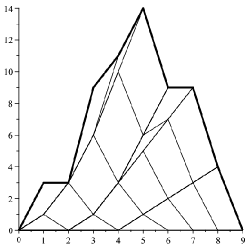
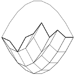
Figure 1: Tilings of the graph of $k\mapsto\operatorname{mult}_{k}{\sigma}$ and of the Elnitsky’s polygon $\mathcal{P}_{\sigma}$ for $\sigma=[429681735]\in S_{9}$ corresponding to the commutation class of the reduced word $\sigma=a_{1}a_{3}a_{4}a_{5}a_{4}a_{3}a_{2}a_{1}a_{6}a_{5}a_{7}a_{6}a_{5}a_{4}a_{3}a_{8}a_{7}a_{6}a_{5}$.

3 Signed permutations

In this section we study the lift $\widetilde{\operatorname{B}}^{+}_{n+1}\subset\operatorname{Spin}_{n+1}$ of the index two subgroup $\operatorname{B}^{+}_{n+1}=\operatorname{B}_{n+1}\cap\operatorname{SO}_{n+1}$ of the hyperoctahedral group $\operatorname{B}_{n+1}$. Recall the surjective group homomorphism $\sigma:\widetilde{\operatorname{B}}^{+}_{n+1}\to S_{n+1}$, $z\mapsto\sigma_{z}$, and its kernel $\operatorname{Quat}_{n+1}$.

The group $\operatorname{B}_{n+1}$ is a Coxeter group (whence the notation) with generators $P_{a_{1}},\ldots,P_{a_{n}},R$, where $e_{k}^{\top}R=(-1)^{[k=1]}e_{k}^{\top}$, but we do not use this presentation (the bracket $[k=1]$ is another example of Iverson bracket, already seen in Equation 7). Rather, consider the elements $\acute{a}_{1},\ldots,\acute{a}_{n}\in\widetilde{\operatorname{B}}^{+}_{n+1}$ defined in the introduction by $\acute{a}_{j}=\exp\left(\frac{\pi}{2}{\mathfrak{a}}_{j}\right)$, ${\mathfrak{a}}_{j}=e_{j+1}e_{j}^{\top}-e_{j}e_{j+1}^{\top}\in\operatorname{\mathfrak{so}}_{n+1}\approx\mathfrak{spin}_{n+1}$. Also, recall the elements $\hat{a}_{j}=\acute{a}_{j}^{2}\in\operatorname{Quat}_{n+1}$.

Lemma 3.1.

The following identities hold:

$$|i-j|\neq 1\quad\implies\quad\acute{a}_{j}\acute{a}_{i}=\acute{a}_{i}\acute{a}_{j},\;\hat{a}_{j}\acute{a}_{i}=\acute{a}_{i}\hat{a}_{j},\;\hat{a}_{j}\hat{a}_{i}=\hat{a}_{i}\hat{a}_{j};$$

$$\acute{a}_{i}\acute{a}_{i+1}\acute{a}_{i}=\acute{a}_{i+1}\acute{a}_{i}\acute{a}_{i+1};\qquad(\acute{a}_{i})^{-1}\acute{a}_{i+1}(\acute{a}_{i})^{-1}=\acute{a}_{i+1}(\acute{a}_{i})^{-1}\acute{a}_{i+1};$$

$$|i-j|=1\quad\implies\quad\hat{a}_{j}\acute{a}_{i}=(\acute{a}_{i})^{-1}\hat{a}_{j},\;\hat{a}_{j}\hat{a}_{i}=-\hat{a}_{i}\hat{a}_{j}.$$

Proof.

These are simple computations with any point of view; they are particularly easy using the Clifford algebra $\operatorname{Cl}_{n+1}^{0}$, as discussed in the introduction near Equation 1. ∎

Each element $q\in\operatorname{Quat}_{n+1}$ can be written uniquely as

$$q=\pm\hat{a}_{1}^{\varepsilon_{1}}\hat{a}_{2}^{\varepsilon_{2}}\cdots\hat{a}_{n}^{\varepsilon_{n}},\quad\varepsilon_{i}\in\{0,1\}.$$

In particular, the elements $\hat{a}_{1},\ldots,\hat{a}_{n}$ generate $\operatorname{Quat}_{n+1}$. Furthermore, if $z\in\widetilde{\operatorname{B}}_{n+1}^{+}$ and $\sigma_{z}=a_{i_{1}}\cdots a_{i_{k}}\in S_{n+1}$, take $z_{1}=\acute{a}_{i_{1}}\cdots\acute{a}_{i_{k}}\in\widetilde{\operatorname{B}}_{n+1}^{+}$: we have $\sigma_{z}=\sigma_{z_{1}}$ and therefore $z=qz_{1}$ with $q\in\operatorname{Quat}_{n+1}$. In particular, the elements $\acute{a}_{1},\ldots,\acute{a}_{n}$ generate $\widetilde{\operatorname{B}}_{n+1}^{+}$. We make this construction more systematic.

Lemma 3.2.

If $\sigma\in S_{n+1}$ is expressed by two reduced words $\sigma=a_{i_{1}}\cdots a_{i_{k}}=a_{j_{1}}\cdots a_{j_{k}}$ then $\acute{a}_{i_{1}}\cdots\acute{a}_{i_{k}}=\acute{a}_{j_{1}}\cdots\acute{a}_{j_{k}}$.

Proof.

Both moves (as in Equations 5 and 6) are taken care of by Lemma 3.1. ∎

Let $\grave{a}_{i}=(\acute{a}_{i})^{-1}$. For $\sigma\in S_{n+1}$, take a reduced word $\sigma=a_{i_{1}}\cdots a_{i_{k}}$ and set

$$\operatorname{acute}(\sigma)=\acute{\sigma}=\acute{a}_{i_{1}}\cdots\acute{a}_{i_{k}};\qquad\operatorname{grave}(\sigma)=\grave{\sigma}=\grave{a}_{i_{1}}\cdots\grave{a}_{i_{k}},$$

as in Equation 2. Lemma 3.2 shows that the maps $\operatorname{acute},\operatorname{grave}:S_{n+1}\to\widetilde{\operatorname{B}}_{n+1}^{+}$ are well defined. Notice that these maps are not homomorphisms. Similarly, non-reduced words do not work in the above formulas for $\acute{\sigma}$ and $\grave{\sigma}$. Also, define

$$\operatorname{hat}(\sigma)=\hat{\sigma}=\acute{\sigma}(\grave{\sigma})^{-1}=\acute{a}_{i_{1}}\cdots\acute{a}_{i_{k}}\acute{a}_{i_{k}}\cdots\acute{a}_{i_{1}},$$

so that $\hat{\sigma}\in\operatorname{Quat}_{n+1}$ for all $\sigma\in S_{n+1}$. Notice that these notations are consistent with the previously introduced special cases $\acute{a}_{i}$ and $\hat{a}_{i}$.

Lemma 3.3.

Consider $\sigma\in S_{n+1}$ and set $\acute{P}=\Pi(\acute{\sigma})\in\operatorname{B}^{+}_{n+1}$. We have

$$e^{\top}_{i}\acute{P}=(-1)^{\operatorname{inv}_{i}(\sigma)}e^{\top}_{i^{\sigma}}\,,\qquad\acute{P}e_{j}=(-1)^{\operatorname{inv}_{j^{\sigma^{-1}}}(\sigma)}e_{j^{\sigma^{-1}}}$$

and therefore $\acute{P}_{ij}=e^{\top}_{i}\acute{P}e_{j}=(-1)^{\operatorname{inv}_{i}(\sigma)}[j=i^{\sigma}].$ The nonzero entries of $\hat{P}=\Pi(\hat{\sigma})\in\operatorname{Diag}_{n+1}^{+}$ are

$$(\hat{P})_{ii}=(-1)^{\operatorname{inv}_{i}(\sigma)+\operatorname{inv}_{i^{\sigma}}(\sigma^{-1})}=(-1)^{i+i^{\sigma}}=(-1)^{\operatorname{mult}_{i-1}(\sigma)+\operatorname{mult}_{i}(\sigma)}.$$

We also have $\hat{\sigma}=\pm\hat{a}_{1}^{\operatorname{mult}_{1}(\sigma)}\cdots\hat{a}_{n}^{\operatorname{mult}_{n}(\sigma)}$.

The expression $[j=i^{\sigma}]$ in the statement above is another use of Iverson bracket. Recall that $\operatorname{inv}_{i}(\sigma)=|\operatorname{Inv}_{i}(\sigma)|$, where $\operatorname{Inv}_{i}(\sigma)$ is defined in Equation 8.

Proof.

The first expression for the diagonal entries of $\hat{P}=\Pi(\acute{\sigma})\Pi(\operatorname{acute}(\sigma^{-1}))$ follows directly from the first two formulae, which we now prove by induction on $\operatorname{inv}(\sigma)$. The base cases $\operatorname{inv}(\sigma)\leq 1$ are easy. Assume $\sigma_{1}\vartriangleleft\sigma=a_{k}\sigma_{1}$, so that $\acute{P}=\Pi(\acute{a}_{k})\acute{P}_{1}$, where $\acute{P}_{1}=\Pi(\acute{\sigma}_{1})$. By the induction hypotheses we have

$$e^{\top}_{i}\acute{P}=e^{\top}_{i}\Pi(\acute{a}_{k})\acute{P}_{1}=(-1)^{\operatorname{inv}_{i}(a_{k})}e^{\top}_{i^{a_{k}}}\acute{P}_{1}=(-1)^{\operatorname{inv}_{i}(a_{k})+\operatorname{inv}_{i^{a_{k}}}(\sigma_{1})}e^{\top}_{i^{\sigma}}.$$

To see that $\operatorname{inv}_{i}(\sigma)=\operatorname{inv}_{i}(a_{k})+\operatorname{inv}_{i^{a_{k}}}(\sigma_{1})$ for all values of $i\in\llbracket n+1\rrbracket$, consider separately the cases $i<k$, $i=k$, $i=k+1$ and $i>k+1$. The second formula is similar. The alternate expressions for $\hat{P}_{ii}$ are obtained via Lemma 2.5. The last of these expressions imply that $\hat{P}=\Pi(\hat{\sigma})=\Pi(\hat{a}_{1}^{\operatorname{mult}_{1}(\sigma)}\cdots\hat{a}_{n}^{\operatorname{mult}_{n}(\sigma)})$, and therefore, $\hat{\sigma}=\pm\hat{a}_{1}^{\operatorname{mult}_{1}(\sigma)}\cdots\hat{a}_{n}^{\operatorname{mult}_{n}(\sigma)}$. ∎

If $\sigma_{1}\vartriangleleft\sigma_{0}=a_{i}\sigma_{1}$ then, by definition,

$$\acute{\sigma}_{0}=\acute{a}_{i}\acute{\sigma}_{1},\qquad\hat{\sigma}_{0}=\acute{a}_{i}\hat{\sigma}_{1}\acute{a}_{i}.$$

We show how to obtain a different recursive formula for $\hat{\sigma}_{0}$.

Lemma 3.4.

Let $q\in\operatorname{Quat}_{n+1}$ and $E=\Pi(q)\in\operatorname{Diag}^{+}_{n+1}$; write

$$q=\pm\hat{a}_{1}^{\varepsilon_{1}}\cdots\hat{a}_{n}^{\varepsilon_{n}},\quad\varepsilon_{1},\ldots,\varepsilon_{n}\in{\mathbb{Z}}.$$

With the convention $\varepsilon_{0}=\varepsilon_{n+1}=0$, we have:

1. If $\varepsilon_{i-1}+\varepsilon_{i+1}$ is odd then $q\acute{a}_{i}=\grave{a}_{i}q$, $q\hat{a}_{i}=-\hat{a}_{i}q$, $E_{i+1,i+1}=-E_{i,i}$.

2. If $\varepsilon_{i-1}+\varepsilon_{i+1}$ is even then $q\acute{a}_{i}=\acute{a}_{i}q$, $q\hat{a}_{i}=\hat{a}_{i}q$, $E_{i+1,i+1}=E_{i,i}$.

Proof.

From Lemma 3.1,

$$\hat{a}_{j}\acute{a}_{i}=\begin{cases}\acute{a}_{i}\hat{a}_{j},&|i-j|\neq 1,\\ \grave{a}_{i}\hat{a}_{j},&|i-j|=1;\end{cases}\qquad\hat{a}_{j}\grave{a}_{i}=\begin{cases}\grave{a}_{i}\hat{a}_{j},&|i-j|\neq 1,\\ \acute{a}_{i}\hat{a}_{j},&|i-j|=1;\end{cases}$$

these imply the formulas for $q\acute{a}_{i}$. We then have, for $\varepsilon_{i-1}+\varepsilon_{i+1}$ even,

$$q\hat{a}_{i}=q\acute{a}_{i}\acute{a}_{i}=\acute{a}_{i}q\acute{a}_{i}=\acute{a}_{i}\acute{a}_{i}q=\hat{a}_{i}q$$

and, for $\varepsilon_{i-1}+\varepsilon_{i+1}$ odd,

$$q\hat{a}_{i}=q\acute{a}_{i}\acute{a}_{i}=\grave{a}_{i}q\acute{a}_{i}=\grave{a}_{i}\grave{a}_{i}q=-\hat{a}_{i}q.$$

Finally, notice that $\varepsilon_{i-1}+\varepsilon_{i+1}$ even implies $E\Pi(\acute{a}_{i})=\Pi(\acute{a}_{i})E$ and therefore $E_{i+1,i+1}=E_{i,i}$; conversely, $\varepsilon_{i-1}+\varepsilon_{i+1}$ odd implies $E\Pi(\acute{a}_{i})=\Pi((\acute{a}_{i})^{-1})E=(\Pi(\acute{a}_{i}))^{-1}E$ and therefore $E_{i+1,i+1}=-E_{i,i}$. ∎

Lemma 3.5.

Let $\sigma_{1}\vartriangleleft\sigma_{0}=a_{i}\sigma_{1}=\sigma_{1}(j_{0}j_{1})$, $\delta=j_{1}-j_{0}$.

1. If $\delta$ is odd then $\hat{\sigma}_{1}\hat{a}_{i}=\hat{a}_{i}\hat{\sigma}_{1}$ and $\hat{\sigma}_{0}=\hat{a}_{i}\hat{\sigma}_{1}=\hat{\sigma}_{1}\hat{a}_{i}$.

2. If $\delta$ is even then $\hat{\sigma}_{1}\hat{a}_{i}=-\hat{a}_{i}\hat{\sigma}_{1}$ and $\hat{\sigma}_{0}=\hat{\sigma}_{1}=\hat{a}_{i}\hat{\sigma}_{1}\hat{a}_{i}$.

Proof.

We know (by definition) that $\hat{\sigma}_{0}=\acute{a}_{i}\hat{\sigma}_{1}\acute{a}_{i}$. As in Lemma 3.4, write $\hat{\sigma}_{1}=\pm\hat{a}_{1}^{\varepsilon_{1}}\cdots\hat{a}_{n}^{\varepsilon_{n}}$. We know from Lemma 3.3 that we can take $\varepsilon_{j}=\operatorname{mult}_{j}(\sigma_{1})$. Thus

$$\varepsilon_{i+1}-\varepsilon_{i-1}=(i+1)^{\sigma_{1}}+i^{\sigma_{1}}-(i+1)-i=j_{1}+j_{0}-2i-1\equiv\delta+1\pmod{2}.$$

If $\delta$ is odd then $\hat{\sigma}_{1}\acute{a}_{i}=\acute{a}_{i}\hat{\sigma}_{1}$ and therefore $\hat{\sigma}_{1}\hat{a}_{i}=\hat{a}_{i}\hat{\sigma}_{1}$ and $\hat{\sigma}_{0}=\hat{a}_{i}\hat{\sigma}_{1}=\hat{\sigma}_{1}\hat{a}_{i}$. If $\delta$ is even then $\hat{\sigma}_{1}\acute{a}_{i}=(\acute{a}_{i})^{-1}\hat{\sigma}_{1}$ and therefore $\hat{\sigma}_{1}\hat{a}_{i}=-\hat{a}_{i}\hat{\sigma}_{1}$ and $\hat{\sigma}_{0}=\hat{\sigma}_{1}=\hat{a}_{i}\hat{\sigma}_{1}\hat{a}_{i}$. ∎

Example 3.6.

Using this result it is easy to compute $\hat{\sigma}_{0}$ given $\sigma_{0}$. Take, say, $\sigma_{0}=[7245136]=[a_{1}a_{2}a_{3}a_{4}a_{3}a_{2}a_{1}a_{5}a_{4}a_{3}a_{6}]$. Take

$$\sigma_{0}=a_{1}\sigma_{1}\vartriangleright\sigma_{1}=[2745136],\qquad\sigma_{1}=a_{2}\sigma_{2}\vartriangleright\sigma_{2}=[2475136],$$

$$\sigma_{2}=a_{3}\sigma_{3}\vartriangleright\sigma_{3}=[2457136],\qquad\sigma_{3}=a_{4}\sigma_{4}\vartriangleright\sigma_{4}=[2451736],$$

$$\sigma_{4}=a_{3}\sigma_{5}\vartriangleright\sigma_{5}=[2415736],\qquad\sigma_{5}=a_{2}\sigma_{6}\vartriangleright\sigma_{6}=[2145736],$$

$$\sigma_{6}=a_{1}\sigma_{7}\vartriangleright\sigma_{7}=[1245736],\qquad\sigma_{7}=a_{5}\sigma_{8}\vartriangleright\sigma_{8}=[1245376],$$

$$\sigma_{8}=a_{4}\sigma_{9}\vartriangleright\sigma_{9}=[1243576],\qquad\sigma_{9}=a_{3}\sigma_{10}\vartriangleright\sigma_{10}=[1234576]=a_{6}.$$

We therefore have

$$\hat{\sigma}_{0} =\hat{a}_{1}\hat{\sigma}_{1}=\hat{a}_{1}\hat{a}_{2}\hat{\sigma}_{2}=\hat{a}_{1}\hat{a}_{2}\hat{\sigma}_{3}=\hat{a}_{1}\hat{a}_{2}\hat{\sigma}_{4}=\hat{a}_{1}\hat{a}_{2}\hat{\sigma}_{5}=$$

$$=\hat{a}_{1}\hat{a}_{2}\hat{a}_{2}\hat{\sigma}_{6}=\hat{a}_{1}\hat{a}_{2}\hat{a}_{2}\hat{a}_{1}\hat{\sigma}_{7}=\hat{\sigma}_{7}=\hat{\sigma}_{8}=\hat{\sigma}_{9}=\hat{a}_{3}\hat{\sigma}_{10}=\hat{a}_{3}\hat{a}_{6},$$

completing the computation. $\diamond$

Example 3.7.

We have that $\eta=a_{1}a_{2}a_{1}a_{3}a_{2}a_{1}\cdots a_{n}a_{n-1}\cdots a_{2}a_{1}$ is a reduced word so that $\acute{\eta}=\acute{a}_{1}\acute{a}_{2}\acute{a}_{1}\acute{a}_{3}\acute{a}_{2}\acute{a}_{1}\cdots\acute{a}_{n}\acute{a}_{n-1}\cdots\acute{a}_{2}\acute{a}_{1}$ and $\hat{\eta}=(\acute{\eta})^{2}$. From Lemma 3.3, we have $\Pi(\hat{\eta})=(-1)^{n}\;I$ and

$$\Pi(\acute{\eta})=\begin{pmatrix}&&&\iddots\\ &&1&\\ &-1&&\\ 1&&&\end{pmatrix},\qquad\hat{\eta}=\begin{cases}1,&n\equiv 0,6\pmod{8},\\ -1,&n\equiv 2,4\pmod{8},\\ \hat{a}_{1}\hat{a}_{3}\cdots\hat{a}_{n},&n\equiv 1,7\pmod{8},\\ -\hat{a}_{1}\hat{a}_{3}\cdots\hat{a}_{n},&n\equiv 3,5\pmod{8}.\end{cases}$$

Notice the periodicity modulo eight, which also occurs in other contexts. $\diamond$

Remark 3.8.

For all $n>3$, there are $\sigma,\rho\in S_{n+1}\smallsetminus\{e,\eta\}$ such that $\hat{\sigma}=1$ and $\hat{\rho}=\hat{\eta}$: take $\sigma=(1,5)=a_{1}a_{2}a_{3}a_{4}a_{3}a_{2}a_{1}$; we have $\hat{\sigma}=1$, $\operatorname{hat}(\eta\sigma)=\operatorname{hat}(\sigma\eta)=\hat{\eta}$.

No such elements exist in $S_{n+1}$ for $n\in\{2,3\}$. For $n=2$ we have $\hat{\sigma}=\pm 1$ if and only if $\sigma\in\{e,\eta\}$, with $\hat{e}=1$ and $\hat{\eta}=-1$. For $n=3$ we have $\hat{\sigma}=\pm 1$ if and only if $\sigma\in\{e,[1432],[3214],[3412]\}$ with $\hat{e}=1$, $\operatorname{hat}([1432])=\operatorname{hat}([3214])=\operatorname{hat}([3412])=-1$. Also, $\hat{\sigma}=\pm\hat{\eta}$ if and only if $\sigma\in\{[2143],[4123],[2341],\eta\}$, with $\operatorname{hat}([2143])=\operatorname{hat}([4123])=\operatorname{hat}([2341])=\hat{a}\hat{c}$, $\hat{\eta}=-\hat{a}\hat{c}$. $\diamond$

4 Triangular coordinates

Let $\operatorname{Up}_{n+1}^{+}\subset\operatorname{GL}_{n+1}$ be the group of real upper triangular matrices with all diagonal entries strictly positive. Recall the $LU$ decomposition: a matrix $A\in\operatorname{GL}_{n+1}$ can be (uniquely) written as $A=LU$, $L\in\operatorname{Lo}_{n+1}^{1}$ and $U\in\operatorname{Up}_{n+1}^{+}$ provided each of its northwest minor determinants is positive. This condition holds in a contractible open neighborhood of the identity matrix $I$; for $A$ in this set, $L$ and $U$ are smoothly and uniquely defined. We shall be more interested in ${\cal U}_{I}\subset\operatorname{SO}_{n+1}$, the intersection of this neighborhood with $\operatorname{SO}_{n+1}$, which is also a contractible open subset. Let ${\mathbf{L}}:{\cal U}_{I}\to\operatorname{Lo}_{n+1}^{1}$ take $Q\in{\cal U}_{I}$ to the unique $L={\mathbf{L}}(Q)\in\operatorname{Lo}_{n+1}^{1}$ such that there exists $U\in\operatorname{Up}_{n+1}^{+}$ with $Q=LU$: the map ${\mathbf{L}}$ is a diffeomorphism. Indeed, its inverse ${\mathbf{Q}}:\operatorname{Lo}_{n+1}^{1}\to{\cal U}_{I}$ is given by the orthogonal factor in the $QR$ decomposition: given $L\in\operatorname{Lo}_{n+1}^{1}$ let $Q={\mathbf{Q}}(L)\in\operatorname{SO}_{n+1}$ be the unique matrix for which there exists $R\in\operatorname{Up}_{n+1}^{+}$ with $L=QR$.

The set $\Pi^{-1}[{\cal U}_{I}]\subset\operatorname{Spin}_{n+1}$ has two contractible connected components: we call them ${\cal U}_{1}$ and ${\cal U}_{-1}$, where $1\in{\cal U}_{1}$ and $-1\in{\cal U}_{-1}$. We abuse notation and write ${\mathbf{L}}:{\cal U}_{1}\to\operatorname{Lo}_{n+1}^{1}$ and ${\mathbf{Q}}:\operatorname{Lo}_{n+1}^{1}\to{\cal U}_{1}$ for the diffeomorphisms obtained by composition. For $z_{0}\in\operatorname{Spin}_{n+1}$, we set ${\cal U}_{z_{0}}=z_{0}{\cal U}_{1}$, an open contractible neighborhood of $z_{0}$, diffeomorphic to $\operatorname{Lo}^{1}_{n+1}$ under the map $z\mapsto{\mathbf{L}}(z_{0}^{-1}z)$. This map may be seen as a chart, defining triangular coordinates on the open contractible subset ${\cal U}_{z_{0}}\subset\operatorname{Spin}_{n+1}$.

For each $j\in\llbracket n\rrbracket$, let ${\mathfrak{l}}_{j}=e_{j+1}e_{j}^{\top}\in\operatorname{\mathfrak{lo}}^{1}_{n+1}$ be the matrix with only one nonzero entry $({\mathfrak{l}}_{j})_{j+1,j}=1$. Recall that ${\mathfrak{a}}_{j}={\mathfrak{l}}_{j}-{\mathfrak{l}}_{j}^{\top}\in\operatorname{\mathfrak{so}}_{n+1}\approx\mathfrak{spin}_{n+1}$. Let $X_{{\mathfrak{a}}_{j}}$ and $X_{{\mathfrak{l}}_{j}}$ be the left-invariant vector fields in $\operatorname{SO}_{n+1}$ and $\operatorname{Lo}_{n+1}^{1}$ generated by ${\mathfrak{a}}_{j}$ and ${\mathfrak{l}}_{j}$, respectively:

$$X_{{\mathfrak{a}}_{j}}(Q)=Q{\mathfrak{a}}_{j},\qquad X_{{\mathfrak{l}}_{j}}(L)=L{\mathfrak{l}}_{j}.$$

We also denote by $X_{{\mathfrak{a}}_{j}}$ the corresponding left-invariant vector field in $\operatorname{Spin}_{n+1}$.

Lemma 4.1.

The diffeomorphisms ${\mathbf{L}}:{\cal U}_{I}\to\operatorname{Lo}_{n+1}^{1}$ and ${\mathbf{Q}}:\operatorname{Lo}_{n+1}^{1}\to{\cal U}_{I}\subset\operatorname{SO}_{n+1}$ take the vector fields $X_{{\mathfrak{a}}_{j}}$ and $X_{{\mathfrak{l}}_{j}}$ to smooth positive multiples of each other. A similar statement holds for ${\mathbf{L}}:{\cal U}_{1}\to\operatorname{Lo}_{n+1}^{1}$ and ${\mathbf{Q}}:\operatorname{Lo}_{n+1}^{1}\to{\cal U}_{1}\subset\operatorname{Spin}_{n+1}$.

Proof.

Given $Q_{0}\in{\cal U}_{I}$, take a short arc of the integral line of $X_{{\mathfrak{a}}_{j}}$ through $Q_{0}$: let $\epsilon>0$ be sufficiently small so that $Q(t)=Q_{0}\exp(t{\mathfrak{a}}_{j})\in{\cal U}_{I}$ for $-\epsilon<t<\epsilon$. Also write ${\mathbf{L}}(Q(t))=L(t)\in\operatorname{Lo}^{1}_{n+1}$, so that $L(t)=Q(t)R(t)$ for a smooth path $R:(-\epsilon,\epsilon)\to\operatorname{Up}^{+}_{n+1}$. Differentiating the last equation, we have

$$(L(t))^{-1}L^{\prime}(t)=(R(t))^{-1}{\mathfrak{a}}_{j}R(t)+(R(t))^{-1}R^{\prime}(t).$$

Since the left hand side is in $\operatorname{\mathfrak{lo}}^{1}_{n+1}$ and the rightmost summand of the right hand side is in $\operatorname{\mathfrak{up}}^{+}_{n+1}$, it is readily seen that $L^{\prime}(t)=(R(t)_{jj}/R(t)_{j+1,j+1})L(t){\mathfrak{l}}_{j}$. ∎

Recall from the introduction that a locally convex curve is an absolutely continuous map $\Gamma:J\to\operatorname{Spin}_{n+1}$ such that, for all $t\in J$ for which the derivative exists, the logarithmic derivative $(\Gamma(t))^{-1}\Gamma^{\prime}(t)\in\mathfrak{spin}_{n+1}$ is a positive linear combination of ${\mathfrak{a}}_{1},\ldots,{\mathfrak{a}}_{n}$. Similarly, a map $\Gamma:J\to\operatorname{Lo}_{n+1}^{1}$ is called a convex curve if it is absolutely continuous and, for all $t\in J$ for which the derivative exists, the logarithmic derivative $(\Gamma(t))^{-1}\Gamma^{\prime}(t)$ is a positive linear combination of ${\mathfrak{l}}_{1},\ldots,{\mathfrak{l}}_{n}$.

Example 4.2.

Consider ${\mathfrak{h}}_{L},{\mathfrak{n}}\in\operatorname{\mathfrak{lo}}^{1}_{n+1}$ and ${\mathfrak{h}}\in\operatorname{\mathfrak{so}}_{n+1}\approx\mathfrak{spin}_{n+1}$ given by

$${\mathfrak{h}}_{L}=\sum_{j\in\llbracket n\rrbracket}\sqrt{j(n+1-j)}\;{\mathfrak{l}}_{j},\quad{\mathfrak{n}}=\sum_{j\in\llbracket n\rrbracket}{\mathfrak{l}}_{j},\quad{\mathfrak{h}}={\mathfrak{h}}_{L}-{\mathfrak{h}}_{L}^{\top}$$

We have

$$[{\mathfrak{h}}_{L},{\mathfrak{h}}_{L}^{\top}]=\sum^{n}_{k=0}(2k-n)e_{k+1}e^{\top}_{k+1},\quad[{\mathfrak{h}}_{L},[{\mathfrak{h}}_{L},{\mathfrak{h}}_{L}^{\top}]]=-2{\mathfrak{h}}_{L},\quad[{\mathfrak{h}}_{L}^{\top},[{\mathfrak{h}}_{L},{\mathfrak{h}}_{L}^{\top}]]=2{\mathfrak{h}}_{L}^{\top},$$

so that $[{\mathfrak{h}}_{L},{\mathfrak{h}}_{L}^{\top}]=\operatorname{diag}(-n,-n+2,\cdots,n-2,n)$. For $n=1$ and $\theta\in(-\frac{\pi}{2},\frac{\pi}{2})$,

$$\exp(\theta({\mathfrak{h}}_{L}-{\mathfrak{h}}_{L}^{\top}))=\exp(\tan(\theta){\mathfrak{h}}_{L})\exp(\log(\sec(\theta))[{\mathfrak{h}}_{L},{\mathfrak{h}}_{L}^{\top}])\exp(-\tan(\theta){\mathfrak{h}}_{L}^{\top}).$$ (9)

The symmetric product induces a Lie algebra homomorphism $S:\operatorname{\mathfrak{sl}}_{2}\to\operatorname{\mathfrak{sl}}_{n+1}$ with $S({\mathfrak{h}}_{L})={\mathfrak{h}}_{L}$ (that is, taking ${\mathfrak{h}}_{L}\in{\mathbb{R}}^{2\times 2}$ to ${\mathfrak{h}}_{L}\in{\mathbb{R}}^{(n+1)\times(n+1)}$) and $S({\mathfrak{h}}_{L}^{\top})={\mathfrak{h}}_{L}^{\top}$. We therefore also have a Lie group homomorphism $S:\widetilde{\operatorname{SL}_{2}}\to\widetilde{\operatorname{SL}_{n+1}}$, $S(\exp(t{\mathfrak{u}}))=\exp(tS({\mathfrak{u}}))$ for all ${\mathfrak{u}}\in\operatorname{\mathfrak{sl}}_{2}$, $t\in{\mathbb{R}}$. Equation 9 therefore holds for any value of $n$. We therefore have $\exp(\theta{\mathfrak{h}})\in{\cal U}_{1}$ for all $\theta\in(-\frac{\pi}{2},\frac{\pi}{2})$, with

$${\mathbf{L}}(\exp(\theta{\mathfrak{h}}))=\exp(\tan(\theta){\mathfrak{h}}_{L});\qquad{\mathbf{Q}}(\exp(t{\mathfrak{h}}_{L}))=\exp(\arctan(t){\mathfrak{h}}).$$

Also, the equation $\exp(\frac{\pi}{2}{\mathfrak{h}})=\acute{\eta}$, which is trivially true for $n=1$, can be obtained for arbitrary $n$ using the Lie group homomorphism $S$ above and noticing that $S(\acute{\eta})=\acute{\eta}$.

For $z_{0}\in\operatorname{Spin}_{n+1}$, the curve $\Gamma_{z_{0},{\mathfrak{h}}}(t)=z_{0}\exp(t{\mathfrak{h}})$ is locally convex and satisfies $\Gamma_{z_{0},{\mathfrak{h}}}(\frac{\pi}{2})=z_{0}\acute{\eta}$, $\Gamma_{z_{0},{\mathfrak{h}}}(\pi)=z_{0}\hat{\eta}$. For $L_{0}\in\operatorname{Lo}^{1}_{n+1}$, the curves $\Gamma_{L_{0},{\mathfrak{h}}_{L}}(t)=L_{0}\exp(t{\mathfrak{h}}_{L})$ and $\Gamma_{L_{0},{\mathfrak{n}}}(t)=L_{0}\exp(t{\mathfrak{n}})$ are convex. Notice that the $(i,j)$ entry of either $\Gamma_{L_{0},{\mathfrak{h}}_{L}}(t)$ or $\Gamma_{L_{0},{\mathfrak{n}}}(t)$ is a polynomial of degree $(i-j)$ in the variable $t$. $\diamond$

One advantage of working with triangular coordinates is that there is then a simple integration formula. Indeed, given a convex curve $\Gamma:J\to\operatorname{Lo}_{n+1}^{1}$, write $(\Gamma(t))^{-1}\Gamma^{\prime}(t)=\sum_{i}\beta_{i}(t){\mathfrak{l}}_{i}$. The positive functions $\beta_{1},\ldots,\beta_{n}:J\to(0,+\infty)$ are then integrable in compact subintervals of $J$. Fixed $t_{0}\in J$, we have

$$(\Gamma(t))_{i+1,i}=(\Gamma(t_{0}))_{i+1,i}+\int_{t_{0}}^{t}\beta_{i}(\tau)d\tau.$$

More generally,

$$((\Gamma(t_{0}))^{-1}\Gamma(t))_{i+l,i}=\int_{t_{0}\leq\tau_{1}\leq\cdots\leq\tau_{l}\leq t}\beta_{i+l-1}(\tau_{1})\cdots\beta_{i}(\tau_{l})d\tau_{1}\cdots d\tau_{l}.$$ (10)

We have, therefore, the following equivalent definition: a map $\Gamma:[t_{0},t_{1}]\to\operatorname{Lo}_{n+1}^{1}$ is a convex curve if and only if there exist finite absolutely continuous (positive) Borel measures $\mu_{1},\ldots,\mu_{n}$ on $J=[t_{0},t_{1}]$ such that, for any index $i\in\llbracket n\rrbracket$ and for any nondegenerate interval $\tilde{J}\subseteq J$, $\mu_{i}(\tilde{J})>0$, and such that, for $t_{0}\leq t\leq t_{1}$,

$$((\Gamma(t_{0}))^{-1}\Gamma(t))_{i+l,i} =(\mu_{i+l-1}\times\cdots\times\mu_{i})(\Delta),$$ (11)

$$\Delta =\{(\tau_{1},\ldots,\tau_{l})\in[t_{0},t]^{k}\;|\;t_{0}\leq\tau_{1}\leq\cdots\leq\tau_{l}\leq t\}.$$

It follows from Lemma 4.1 that a map $\Gamma:J\to\operatorname{Spin}_{n+1}$ is locally convex if and only if, near any point $t_{\bullet}\in J$, there is a system of triangular coordinates $\Gamma_{L}(t)={\mathbf{L}}(z_{0}^{-1}\Gamma(t))$ with $\Gamma_{L}$ convex in the previous sense. The reason for calling curves such as $\Gamma_{L}$ convex is that the space curve $\gamma:J\to{\mathbb{R}}^{n+1}$ given by $\gamma(t)=\Pi(z_{0}{\mathbf{Q}}(\Gamma_{L}(t)))e_{1}$ is convex in the geometric sense explained in the introduction.

Let $\llbracket n+1\rrbracket^{(k)}$ be the set of subsets ${\mathbf{i}}\subseteq\llbracket n+1\rrbracket$ with $\operatorname{card}({\mathbf{i}})=k$; let $\sum({\mathbf{i}})$ be the sum of the elements of the set ${\mathbf{i}}$. The $k$-th exterior (or alternating) power $\Lambda^{k}({\mathbb{R}}^{n+1})$ has a basis indexed by ${\mathbf{i}}\in\llbracket n+1\rrbracket^{(k)}$. For ${\mathbf{i}}_{0},{\mathbf{i}}_{1}\in\llbracket n+1\rrbracket^{(k)}$, write:

$${\mathbf{i}}_{0}\overset{j}{\to}{\mathbf{i}}_{1}\quad\iff\quad j\in{\mathbf{i}}_{1},\;j+1\notin{\mathbf{i}}_{1},\;{\mathbf{i}}_{0}=({\mathbf{i}}_{1}\smallsetminus\{j\})\cup\{j+1\}.$$

Notice that ${\mathbf{i}}_{0}\overset{j}{\to}{\mathbf{i}}_{1}$ implies $\sum({\mathbf{i}}_{0})=1+\sum({\mathbf{i}}_{1})$. With respect to the basis above, the matrix of the linear endomorphism $\Lambda^{k}({\mathfrak{l}}_{j})\in\mathfrak{gl}(\Lambda^{k}({\mathbb{R}}^{n+1}))$ given by

$$\Lambda^{k}({\mathfrak{l}}_{j})(v_{1}\wedge\cdots\wedge v_{k})=\sum_{i\in\llbracket k\rrbracket}v_{1}\wedge\cdots\wedge{\mathfrak{l}}_{j}(v_{i})\wedge\cdots\wedge v_{k}$$

has nonzero entries all equal $1$ and in positions $({\mathbf{i}}_{0},{\mathbf{i}}_{1})$ such that ${\mathbf{i}}_{0}\overset{j}{\to}{\mathbf{i}}_{1}$. Write ${\mathbf{i}}_{1}\vartriangleleft{\mathbf{i}}_{0}$ if there exists $j$ such that ${\mathbf{i}}_{0}\overset{j}{\to}{\mathbf{i}}_{1}$ and define a partial order in $\llbracket n+1\rrbracket^{(k)}$ by taking the transitive closure. Equivalently, for ${\mathbf{i}}_{j}=\{i_{j1}<i_{j2}<\cdots<i_{jk}\}$ we have

$${\mathbf{i}}_{1}\leq{\mathbf{i}}_{0}\quad\iff\quad i_{11}\leq i_{01},\;i_{12}\leq i_{02},\;\cdots\;,i_{1k}\leq i_{0k}.$$

If ${\mathbf{i}}_{0}\geq{\mathbf{i}}_{1}$, $\sum({\mathbf{i}}_{0})=l+\sum({\mathbf{i}}_{1})$, write

$${\mathbf{i}}_{0}\overset{(j_{1},\ldots,j_{l})}{\longrightarrow}{\mathbf{i}}_{1}\quad\iff\quad\exists{\mathbf{j}}_{0},\ldots,{\mathbf{j}}_{l},\;{\mathbf{i}}_{0}={\mathbf{j}}_{0}\overset{j_{1}}{\to}{\mathbf{j}}_{1}\to\cdots\to{\mathbf{j}}_{l-1}\overset{j_{l}}{\to}{\mathbf{j}}_{l}={\mathbf{i}}_{1};$$

notice that given ${\mathbf{i}}_{0}$ and ${\mathbf{i}}_{1}$ there may exist many such $l$-tuples $(j_{1},\ldots,j_{l})$. Order the indices ${\mathbf{i}}$ consistently with the partial order introduced above (or, more directly, order the subsets ${\mathbf{i}}$ increasingly in the sum of their elements). The matrix $\Lambda^{k}({\mathfrak{l}}_{i})$ is then strictly lower triangular.

If $L\in\operatorname{Lo}_{n+1}^{1}$ and ${\mathbf{i}}_{0},{\mathbf{i}}_{1}\in\llbracket n+1\rrbracket^{(k)}$, define $L_{{\mathbf{i}}_{0},{\mathbf{i}}_{1}}$ to be the $k\times k$ submatrix of $L$ obtained by selecting the rows in ${\mathbf{i}}_{0}$ and the columns in ${\mathbf{i}}_{1}$. The $({\mathbf{i}}_{0},{\mathbf{i}}_{1})$ entry of $\Lambda^{k}(L)$ is $\det(L_{{\mathbf{i}}_{0},{\mathbf{i}}_{1}})$. Clearly, ${\mathbf{i}}_{0}\not\geq{\mathbf{i}}_{1}$ implies $\det(L_{{\mathbf{i}}_{0},{\mathbf{i}}_{1}})=0$; also, $L_{{\mathbf{i}},{\mathbf{i}}}$ is lower triangular with diagonal entries equal to $1$ and therefore $\det(L_{{\mathbf{i}},{\mathbf{i}}})=1$. The matrix $\Lambda^{k}(L)$ is therefore lower triangular with diagonal entries equal to $1$. Furthermore, the map $\Lambda^{k}:\operatorname{Lo}_{n+1}^{1}\to\operatorname{Lo}_{\binom{n+1}{k}}^{1}$ is a group homomorphism. The following result generalizes Equations 10 and 11 above.

Lemma 4.3.

Let $\Gamma:[t_{0},t_{1}]\to\operatorname{Lo}_{n+1}^{1}$ be a convex curve with $\Gamma(t_{0})=L_{0}$ and let $\beta_{i}(t)=((\Gamma(t))^{-1}\Gamma^{\prime}(t))_{i+1,i}$, $\mu_{i}(J)=\int_{J}\beta_{i}(t)dt$. Let ${\mathbf{i}}_{0},{\mathbf{i}}_{1}\in\llbracket n+1\rrbracket^{(k)}$ with ${\mathbf{i}}_{0}\geq{\mathbf{i}}_{1}$ and $l=\sum({\mathbf{i}}_{0})-\sum({\mathbf{i}}_{1})$. Then

$$\det((L_{0}^{-1}\Gamma(t))_{{\mathbf{i}}_{0},{\mathbf{i}}_{1}}) =(\Lambda^{k}(L_{0}^{-1}\Gamma(t)))_{{\mathbf{i}}_{0},{\mathbf{i}}_{1}}=\sum_{{\mathbf{i}}_{0}\overset{(j_{1},\ldots,j_{l})}{\longrightarrow}{\mathbf{i}}_{1}}(\mu_{j_{1}}\times\cdots\times\mu_{j_{l}})(\Delta);$$

$$\Delta =\{(\tau_{1},\ldots,\tau_{l})\in[t_{0},t]^{l}\;|\;t_{0}\leq\tau_{1}\leq\cdots\leq\tau_{l}\leq t\}.$$

Proof.

These are straightforward computations. ∎

5 Totally positive matrices

A matrix $L\in\operatorname{Lo}_{n+1}^{1}$ is totally positive if for all $k\in\llbracket n+1\rrbracket$ and for all indices ${\mathbf{i}}_{0},{\mathbf{i}}_{1}\in\llbracket n+1\rrbracket^{(k)}$,

$${\mathbf{i}}_{0}\geq{\mathbf{i}}_{1}\quad\implies\quad\det(L_{{\mathbf{i}}_{0},{\mathbf{i}}_{1}})>0.$$

Let $\operatorname{Pos}_{\eta}\subset\operatorname{Lo}_{n+1}^{1}$ be the set of totally positive matrices. In the notation of [4], $G=N=\operatorname{Up}^{1}_{n+1}$ and $N_{>0}=\operatorname{Pos}_{\eta}^{\top}$.

For each $j\in\llbracket n\rrbracket$, let $\lambda_{j}(t)=\exp(t{\mathfrak{l}}_{j})$: for any reduced word $\eta=a_{i_{1}}a_{i_{2}}\cdots a_{i_{m}}$, $m=\operatorname{inv}(\eta)=n(n+1)/2$, the map

$$(0,+\infty)^{m}\to\operatorname{Pos}_{\eta},\qquad(t_{1},t_{2},\ldots,t_{m})\mapsto\lambda_{i_{1}}(t_{1})\lambda_{i_{2}}(t_{2})\cdots\lambda_{i_{m}}(t_{m})$$

is a diffeomorphism. Moreover, there exists a stratification of its closure $\overline{\operatorname{Pos}_{\eta}}$:

$$\overline{\operatorname{Pos}_{\eta}}=\{L\in\operatorname{Lo}_{n+1}^{1}\;|\;\forall{\mathbf{i}}_{0},{\mathbf{i}}_{1},\;(({\mathbf{i}}_{0}\geq{\mathbf{i}}_{1})\to(\det(L_{{\mathbf{i}}_{0},{\mathbf{i}}_{1}})\geq 0))\}=\bigsqcup_{\sigma\in S_{n+1}}\operatorname{Pos}_{\sigma};$$

$\operatorname{Pos}_{\sigma}\subset\operatorname{Lo}_{n+1}^{1}$ is a smooth manifold of dimension $\operatorname{inv}(\sigma)$, and if $\sigma=a_{i_{1}}\cdots a_{i_{k}}$ is a reduced word (so that $k=\operatorname{inv}(\sigma)$) then the map

$$(0,+\infty)^{k}\to\operatorname{Pos}_{\sigma},\qquad(t_{1},t_{2},\ldots,t_{k})\mapsto\lambda_{i_{1}}(t_{1})\lambda_{i_{2}}(t_{2})\cdots\lambda_{i_{k}}(t_{k})$$

is a diffeomorphism. Equivalently, if $\sigma_{1}\vartriangleleft\sigma_{0}=\sigma_{1}a_{i_{k}}$ then the map

$$\operatorname{Pos}_{\sigma_{1}}\times(0,+\infty)\to\operatorname{Pos}_{\sigma_{0}},\qquad(L,t_{k})\mapsto L\lambda_{i_{k}}(t_{k})$$ (12)

is a diffeomorphism.

Different reduced words yield different diffeomorphisms but the same set $\operatorname{Pos}_{\sigma}$: the equation

$$\lambda_{i}(t_{1})\lambda_{i+1}(t_{2})\lambda_{i}(t_{3})=\lambda_{i+1}\left(\frac{t_{2}t_{3}}{t_{1}+t_{3}}\right)\lambda_{i}(t_{1}+t_{3})\lambda_{i+1}\left(\frac{t_{1}t_{2}}{t_{1}+t_{3}}\right)$$ (13)

provides the transition between adjacent parameterizations (i.e., between reduced words connected by the local move in Equation 6; the local move in Equation 5 corresponds to a mere relabeling).

In general, the sets $\operatorname{Pos}_{\sigma}\subset\operatorname{Lo}_{n+1}^{1}$ are neither subgroups nor semigroups and should not be confused with the subgroups $\operatorname{Lo}_{\sigma}=\operatorname{Lo}_{n+1}^{1}\cap(P_{\sigma}^{-1}\operatorname{Up}_{n+1}^{1}P_{\sigma})$ of Equation 4. For instance, $\operatorname{Pos}_{e}=\{I\}$ consists of a single point and $\operatorname{Pos}_{a_{i}}=\{\lambda_{i}(t),t>0\}$ is an open half line; in this case, $\operatorname{Pos}_{a_{i}}\subset\operatorname{Lo}_{a_{i}}$. For $n=2$ and

$$L(x,y,z)=\begin{pmatrix}1&0&0\\ x&1&0\\ z&y&1\end{pmatrix}$$ (14)

we have

$$\operatorname{Pos}_{ab}=\{L(x,y,0)\;|\;x,y>0\};\qquad\operatorname{Pos}_{ba}=\{L(x,y,xy)\;|\;x,y>0\};$$

$$\operatorname{Pos}_{aba}=\{L(x,y,z)\;|\;x,y>0;\;0<z<xy\}.$$

On the other hand,

$$\operatorname{Lo}_{ab}=\{L(x,0,z)\;|\;x,z\in{\mathbb{R}}\};\qquad\operatorname{Lo}_{ba}=\{L(0,y,z)\;|\;y,z\in{\mathbb{R}}\}.$$

If $L\in\operatorname{Pos}_{\sigma}$ then there exist matrices $U_{1},U_{2}\in\operatorname{Up}_{n+1}$ such that $L=U_{1}P_{\sigma}U_{2}$; in other words, $\operatorname{Pos}_{\sigma}\subseteq{\mathbf{Q}}^{-1}[\operatorname{Bru}_{\sigma}]$. The converse is not at all true, not even if we pay attention to signs of diagonal entries of the matrices $U_{i}$. In [36, 37] it is shown that the set of matrices which admit such a decomposition is almost always disconnected; each cell $\operatorname{Pos}_{\sigma}$ is contractible, and so is its closure $\overline{\operatorname{Pos}_{\sigma}}$; see also Lemma 6.3 below.

Lemma 5.1.

Consider $\sigma\in S_{n+1}$, $k\in\llbracket n+1\rrbracket$ and indices ${\mathbf{i}}_{0},{\mathbf{i}}_{1}\in\llbracket n+1\rrbracket^{(k)}$. If there exists $\sigma_{1}=a_{j_{1}}\cdots a_{j_{l_{1}}}\leq\sigma$, $\operatorname{inv}(\sigma_{1})=l_{1}$, such that ${\mathbf{i}}_{0}\overset{(j_{1},\ldots,j_{l_{1}})}{\longrightarrow}{\mathbf{i}}_{1}$ then, for all $L\in\operatorname{Pos}_{\sigma}$, $(\Lambda^{k}(L))_{{\mathbf{i}}_{0},{\mathbf{i}}_{1}}>0$. Conversely, if no such $\sigma_{1}$ exists then, for all $L\in\operatorname{Pos}_{\sigma}$, $(\Lambda^{k}(L))_{{\mathbf{i}}_{0},{\mathbf{i}}_{1}}=0$.

Proof.

Write a reduced word $\sigma=a_{i_{1}}\cdots a_{i_{l}}$. Assume first that such $\sigma_{1}$ exists and that $j_{1}=i_{x_{1}},\ldots,j_{l_{1}}=i_{x_{l_{1}}}$ (where of course $1\leq x_{1}<\cdots<x_{l_{1}}\leq l$). Set

$${\mathbf{i}}_{0}={\mathbf{j}}_{0}\overset{j_{1}}{\to}{\mathbf{j}}_{1}\to\cdots\to{\mathbf{j}}_{l_{1}-1}\overset{j_{l_{1}}}{\to}{\mathbf{j}}_{l_{1}}={\mathbf{i}}_{1};\qquad L=\lambda_{i_{1}}(t_{1})\cdots\lambda_{i_{l}}(t_{l})\in\operatorname{Pos}_{\sigma}.$$

We have $(\Lambda^{k}(L))_{{\mathbf{i}}_{0},{\mathbf{i}}_{1}}\geq t_{x_{1}}\cdots t_{x_{l_{1}}}>0$, as desired.

Conversely, assume that $L=\lambda_{i_{1}}(t_{1})\cdots\lambda_{i_{l}}(t_{l})$, $(\Lambda^{k}(L))_{{\mathbf{i}}_{0},{\mathbf{i}}_{1}}>0$. We have

$$(\Lambda^{k}(L))_{{\mathbf{i}}_{0},{\mathbf{i}}_{1}}=\sum_{{\mathbf{i}}_{0}={\mathbf{j}}_{0}\geq\cdots\geq{\mathbf{j}}_{l}={\mathbf{i}}_{1}}\left((\Lambda^{k}(\lambda_{i_{1}}(t_{1})))_{{\mathbf{j}}_{0},{\mathbf{j}}_{1}}\cdots(\Lambda^{k}(\lambda_{i_{l}}(t_{l})))_{{\mathbf{j}}_{l-1},{\mathbf{j}}_{l}}\right).$$

Consider $({\mathbf{j}}_{0},\ldots,{\mathbf{j}}_{l})$ such that the above product is positive. Let $x_{1},\ldots,x_{l_{1}}$ be such that ${\mathbf{j}}_{x_{1}-1}>{\mathbf{j}}_{x_{1}},\ldots,{\mathbf{j}}_{x_{l_{1}}-1}>{\mathbf{j}}_{x_{l_{1}}}$: this obtains a reduced word for $\sigma_{1}$. ∎

Lemma 5.2.

Consider $L_{0},L_{1}\in\operatorname{Lo}_{n+1}^{1}$. If $L_{0}\in\operatorname{Pos}_{\sigma_{0}}$ and $L_{1}\in\operatorname{Pos}_{\sigma_{1}}$ then $L_{0}L_{1}\in\operatorname{Pos}_{\sigma_{0}\vee\sigma_{1}}$. Thus, $\operatorname{Pos}_{\sigma_{0}}\operatorname{Pos}_{\sigma_{1}}=\operatorname{Pos}_{\sigma_{0}\vee\sigma_{1}}$.

In particular, if $L_{0}\in\operatorname{Pos}_{\eta}$ and $L_{1}\in\overline{\operatorname{Pos}_{\eta}}$ then $L_{0}L_{1},L_{1}L_{0}\in\operatorname{Pos}_{\eta}$. If $L_{0}\in\overline{\operatorname{Pos}_{\eta}}$ and $L_{1}\in\overline{\operatorname{Pos}_{\eta}}$ then $L_{0}L_{1}\in\overline{\operatorname{Pos}_{\eta}}$.

The operation $\vee$ is the one in Example 2.2.

Proof.

The first claim can be proved by induction on $l=\operatorname{inv}(\sigma_{1})$; the case $l=0$ is trivial. For the case $l=1$, consider $\sigma_{1}=a_{i}$ and two cases. If $\sigma_{0}\vee a_{i}=\sigma_{0}$, we take a reduced word $\sigma_{0}=a_{i_{1}}\cdots a_{i_{k}}$ with $i_{k}=i$. Then

$$L_{0}L_{1}=(\lambda_{i_{1}}(t_{1})\cdots\lambda_{i_{k}}(t_{k}))\lambda_{i}(t)=\lambda_{i_{1}}(t_{1})\cdots\lambda_{i_{k}}(t_{k}+t)\in\operatorname{Pos}_{\sigma_{0}}.$$

The case $\sigma_{0}\vee a_{i}\neq\sigma_{0}$ is even more direct. The induction step is now easy.

The other claims follow from the first, but a direct proof may be instructive: consider ${\mathbf{i}}_{0},{\mathbf{i}}_{1}\in\llbracket n+1\rrbracket^{(k)}$, ${\mathbf{i}}_{0}\geq{\mathbf{i}}_{1}$. If $L_{0}\in\operatorname{Pos}_{\eta}$ and $L_{1}\in\overline{\operatorname{Pos}_{\eta}}$ we have

$$(\Lambda^{k}(L_{0}L_{1}))_{{\mathbf{i}}_{0}{\mathbf{i}}_{1}}=(\Lambda^{k}(L_{0}))_{{\mathbf{i}}_{0}{\mathbf{i}}_{1}}(\Lambda^{k}(L_{1}))_{{\mathbf{i}}_{1}{\mathbf{i}}_{1}}+\sum_{{\mathbf{i}}_{0}\geq{\mathbf{i}}>{\mathbf{i}}_{1}}(\Lambda^{k}(L_{0}))_{{\mathbf{i}}_{0}{\mathbf{i}}}(\Lambda^{k}(L_{1}))_{{\mathbf{i}}{\mathbf{i}}_{1}}>0,$$

as desired; the other cases are similar. ∎

Write $L_{0}\leq L_{1}$ if $L_{0}^{-1}L_{1}\in\overline{\operatorname{Pos}_{\eta}}$ and $L_{0}\ll L_{1}$ if $L_{0}^{-1}L_{1}\in\operatorname{Pos}_{\eta}$; notice that $L_{0}^{-1}L_{1}\in\operatorname{Pos}_{\eta}$ is in general not equivalent to $L_{1}L_{0}^{-1}\in\operatorname{Pos}_{\eta}$. Lemma 5.2 implies that these are partial orders:

$$L_{0}\leq L_{1}\leq L_{2}\;\implies\;L_{0}\leq L_{2};\qquad L_{0}\leq L_{1}\ll L_{2}\;\implies\;L_{0}\ll L_{2}.$$ (15)

Lemma 5.3.

Consider $L_{0},L_{1}\in\operatorname{Lo}_{n+1}^{1}$. We have that $L_{0}\ll L_{1}$ if and only if there exists a convex curve $\Gamma:[0,1]\to\operatorname{Lo}_{n+1}^{1}$ with $\Gamma(0)=L_{0}$ and $\Gamma(1)=L_{1}$.

Proof.

We first prove that the existence of $\Gamma$ implies $L_{0}\ll L_{1}$. Given $\Gamma$ and ${\mathbf{i}}_{0},{\mathbf{i}}_{1}\in\llbracket n+1\rrbracket^{(k)}$ with ${\mathbf{i}}_{0}>{\mathbf{i}}_{1}$, Lemma 4.3 gives us a formula for $(L_{0}^{-1}L_{1})_{{\mathbf{i}}_{0},{\mathbf{i}}_{1}}>0$: $L_{0}^{-1}L_{1}$ is therefore totally positive.

Conversely, let ${\mathfrak{l}}=\sum_{i}c_{i}{\mathfrak{l}}_{i}\in\operatorname{\mathfrak{lo}}_{n+1}^{1}$ for fixed positive $c_{i}$. Consider a small closed ball of radius $r>0$ centered at $L_{0}^{-1}L_{1}$ and contained in $\operatorname{Pos}_{\eta}$, the image of a continuous map $h:{\mathbb{B}}^{m}\to\operatorname{Pos}_{\eta}\subset\operatorname{Lo}_{n+1}^{1}$ with $h(0)=L_{0}^{-1}L_{1}$ such that the topological degree of $h|_{{\mathbb{S}}^{m-1}}$ around $L_{0}^{-1}L_{1}$ equals $+1$ (here $m=\dim(\operatorname{Lo}_{n+1}^{1})$). Consider a fixed reduced word $\eta=a_{i_{1}}\cdots a_{i_{m}}$. Define continuous functions $\tau_{i}:{\mathbb{B}}^{m}\to(0,+\infty)$ such that $h(s)=\lambda_{i_{1}}(\tau_{1}(s))\cdots\lambda_{i_{m}}(\tau_{m}(s))$. For $\epsilon\geq 0$, let

$$\Lambda_{\epsilon}(s)(t)=m\tau_{j}(s){\mathfrak{l}}_{i_{j}}+\epsilon{\mathfrak{l}},\quad t\in\left(\frac{j-1}{m},\frac{j}{m}\right).$$

Integrate to obtain maps

$$\Gamma_{\epsilon}(s):[0,1]\to\operatorname{Lo}_{n+1}^{1},\quad\Gamma_{\epsilon}(s)(0)=L_{0},\quad(\Gamma_{\epsilon}(s)(t))^{-1}(\Gamma_{\epsilon}(s))^{\prime}(t)=\Lambda_{\epsilon}(s)(t).$$

Notice that $\Gamma_{\epsilon}(s)$ is a convex curve if $\epsilon>0$. Define $h_{\epsilon}(s)=L_{0}^{-1}\Gamma_{\epsilon}(s)(1)$: clearly $h_{0}=h$, i.e., $\Gamma_{0}(s)(1)=L_{0}h(s)$. By continuity, there exists $\epsilon>0$ such that for all $s\in{\mathbb{B}}^{m}$ we have $|h_{\epsilon}(s)-h_{0}(s)|<r/2$. The topological degree of $h_{\epsilon}|_{{\mathbb{S}}^{m-1}}$ around $L_{0}^{-1}L_{1}$ equals $+1$. There exists therefore $s_{\epsilon}\in{\mathbb{B}}^{m}$ with $h_{\epsilon}(s_{\epsilon})=L_{0}^{-1}L_{1}$. We have that $\Gamma=\Gamma_{\epsilon}(s_{\epsilon}):[0,1]\to\operatorname{Lo}_{n+1}^{1}$ is a convex curve with $\Gamma(0)=L_{0}$, $\Gamma(1)=L_{1}$. ∎

Remark 5.4.

Minor modifications in the above argument yields a smooth convex curve $\Gamma:[0,1]\to\operatorname{Lo}^{1}_{n+1}$ with $\Gamma(0)=L_{0}$ and $\Gamma(1)=L_{1}$ if $L_{0}\ll L_{1}$. $\diamond$

We know by now that if $L_{0}\in\operatorname{Pos}_{\sigma}$ for $\sigma\neq\eta$ and $\Gamma:[0,1]\to\operatorname{Lo}_{n+1}^{1}$ is a convex curve with $\Gamma(0)=L_{0}$ then $\Gamma(t)\in\operatorname{Pos}_{\eta}$ for all $t>0$. The following lemma shows that, at least from the point of view of certain entries, the curve $\Gamma$ goes in with positive speed.

Lemma 5.5.

Given $\sigma\in S_{n+1}$, $\sigma\neq\eta$, there exist $k\in\llbracket n+1\rrbracket$ and indices ${\mathbf{i}}_{0},{\mathbf{i}}_{1},{\mathbf{i}}_{2}\in\llbracket n+1\rrbracket^{(k)}$ and $j\in\llbracket n\rrbracket$ such that ${\mathbf{i}}_{0}\geq{\mathbf{i}}_{1}>{\mathbf{i}}_{2}$, ${\mathbf{i}}_{1}\overset{j}{\to}{\mathbf{i}}_{2}$ and, for all convex curves $\Gamma:[0,1]\to\operatorname{Lo}_{n+1}^{1}$ with $\Gamma(0)\in\operatorname{Pos}_{\sigma}$ and $\Gamma^{\prime}(0)\neq 0$ (and well defined), if $g(t)=(\Lambda^{k}(\Gamma(t)))_{{\mathbf{i}}_{0},{\mathbf{i}}_{2}}$ then $g(0)=0$ and $g^{\prime}(0)>0$.

Proof.

Consider $k$ and a pair of indices ${\mathbf{i}}_{0}\geq{\mathbf{i}}_{3}$ in $\llbracket n+1\rrbracket^{(k)}$ such that $(\Lambda^{k}(L))_{{\mathbf{i}}_{0},{\mathbf{i}}_{3}}=0$ for $L\in\operatorname{Pos}_{\sigma}$ (see Lemma 5.1). Keep $k$ and ${\mathbf{i}}_{0}$ fixed and search for ${\mathbf{i}}_{2}\leq{\mathbf{i}}_{0}$ maximal such that $(\Lambda^{k}(L))_{{\mathbf{i}}_{0},{\mathbf{i}}_{2}}=0$ for $L\in\operatorname{Pos}_{\sigma}$. Maximality implies that there exists ${\mathbf{i}}_{1}$, ${\mathbf{i}}_{0}\geq{\mathbf{i}}_{1}>{\mathbf{i}}_{2}$ and an index $j$ such that ${\mathbf{i}}_{1}\overset{j}{\to}{\mathbf{i}}_{2}$ and $(\Lambda^{k}(L))_{{\mathbf{i}}_{0},{\mathbf{i}}_{1}}>0$ for $L\in\operatorname{Pos}_{\sigma}$.

Let $L_{0}=\Gamma(0)$, $c_{0}=(\Lambda^{k}(L_{0}))_{{\mathbf{i}}_{0},{\mathbf{i}}_{1}}>0$. Write $h_{j}(t)=(L_{0}^{-1}\Gamma(t))_{j+1,j}$ so that $h_{j}(0)=0$ and $h^{\prime}_{j}(0)=c_{j}>0$ (see Equation 10). Now, $g(0)=0$ and, for $t>0$, it follows from $L_{0}\in\operatorname{Pos}_{\sigma}$ and Lemma 4.3 that

$$g(t)\geq(\Lambda^{k}(L_{0}))_{{\mathbf{i}}_{0},{\mathbf{i}}_{1}}(\Lambda^{k}(L_{0}^{-1}\Gamma(t)))_{{\mathbf{i}}_{1},{\mathbf{i}}_{2}}=c_{0}h_{j}(t)=c_{0}c_{j}(t+o(t))$$

(in Landau’s small-o notation) so that $g^{\prime}(0)\geq c_{0}c_{j}>0$, as desired. ∎

Remark 5.6.

We now present an explicit construction. Given $\sigma\neq\eta$, take $k$ minimal such that $(n-k+2)^{\sigma}\neq k$. Set then $j=(n-k+2)^{\sigma}-1$. Equivalently, $k$ is minimal such that $\Lambda^{k}(L)_{{\mathbf{i}}_{0},{\mathbf{i}}_{3}}=0$ for $L\in\operatorname{Pos}_{\sigma}$, ${\mathbf{i}}_{0}=\{n-k+2,\ldots,n+1\}$ and ${\mathbf{i}}_{3}=\{1,\ldots,k\}$. If we follow the proof of Lemma 5.5, we have ${\mathbf{i}}_{1}=\{1,\ldots,k-1,j+1\}$ and ${\mathbf{i}}_{2}=\{1,\ldots,k-1,j\}$. $\diamond$

For $\sigma=a_{i_{1}}\cdots a_{i_{k}}\in S_{n+1}$ a reduced word, and $t_{1},\ldots,t_{k}\in{\mathbb{R}}\smallsetminus\{0\}$, let

$$L=\lambda_{i_{1}}(t_{1})\lambda_{i_{2}}(t_{2})\cdots\lambda_{i_{k}}(t_{k}).$$ (16)

It is well known [4, 36] that $L\in{\mathbf{Q}}^{-1}[\operatorname{Bru}_{\sigma}]$. Let

$$\operatorname{Neg}_{\sigma} =X\operatorname{Pos}_{\sigma}X=\{L\in\operatorname{Lo}^{1}_{n+1}\,|\,L^{-1}\in\operatorname{Pos}_{\sigma^{-1}}\}$$

$$=\{\lambda_{i_{1}}(t_{1})\lambda_{i_{2}}(t_{2})\cdots\lambda_{i_{k}}(t_{k})\,|\,t_{1},t_{2},\ldots,t_{k}\in(-\infty,0)\}$$

where $X=\operatorname{diag}(1,-1,1,-1,\ldots)$ and $\sigma=a_{i_{1}}a_{i_{2}}\cdots a_{i_{k}}$ is any reduced word (therefore $k=\operatorname{inv}(\sigma)$). Of course, each cell $\operatorname{Neg}_{\sigma}\subset\operatorname{Lo}^{1}_{n+1}$ is a contractible submanifold of dimension $\operatorname{inv}(\sigma)$, forming the stratification

$$\overline{\operatorname{Neg}_{\eta}}=\bigsqcup_{\sigma\in S_{n+1}}\operatorname{Neg}_{\sigma}.$$

Notice that $\overline{\operatorname{Pos}_{\eta}}\cap\overline{\operatorname{Neg}_{\eta}}=\{I\}$.

Lemma 5.7.

Consider an interval $J\subseteq{\mathbb{R}}$ and a convex curve $\Gamma:J\to\operatorname{Lo}_{n+1}^{1}$.

1. If $t_{-1}<t_{0}<t_{1}$ and $\Gamma(t_{0})\in\operatorname{Pos}_{\sigma}\subset\partial\operatorname{Pos}_{\eta}$ for some $\sigma\neq\eta$ then $\Gamma(t_{1})\in\operatorname{Pos}_{\eta}$ and $\Gamma(t_{-1})\notin\overline{\operatorname{Pos}_{\eta}}$.

2. If $t_{-1}<t_{0}<t_{1}$ and $\Gamma(t_{0})\in\operatorname{Neg}_{\sigma}\subset\partial\operatorname{Neg}_{\eta}$ for some $\sigma\neq\eta$ then $\Gamma(t_{-1})\in\operatorname{Neg}_{\eta}$ and $\Gamma(t_{1})\notin\overline{\operatorname{Neg}_{\eta}}$.

3. If $t_{0}<t<t_{1}$ then $\Gamma(t)\in(\Gamma(t_{0})\operatorname{Pos}_{\eta})\cap(\Gamma(t_{1})\operatorname{Neg}_{\eta})$.

Proof.

As in the first item, assume $\Gamma(t_{0})\in\operatorname{Pos}_{\sigma}$, $\sigma\neq\eta$. From Lemma 5.3, $\Gamma(t_{0})\ll\Gamma(t_{1})$ and, by definition, $\Gamma(t_{0})^{-1}\Gamma(t_{1})\in\operatorname{Pos}_{\eta}$. By Lemma 5.2, $\Gamma(t_{1})=\Gamma(t_{0})\Gamma(t_{0})^{-1}\Gamma(t_{1})\in\operatorname{Pos}_{\eta}$, proving the first claim. Assume by contradiction that $\Gamma(t_{-1})\in\overline{\operatorname{Pos}_{\eta}}$: from the claim just proved, $\Gamma(t_{0})\in\operatorname{Pos}_{\eta}$, a contradiction. The second item is analogous. The third item follows from the previous ones. ∎

Lemma 5.8.

Consider a reduced word $a_{i_{1}}\cdots a_{i_{m}}=\eta$; consider

$$L=\lambda_{i_{1}}(t_{1})\cdots\lambda_{i_{m}}(t_{m})\in\operatorname{Pos}_{\eta},\qquad t_{1},\ldots,t_{m}>0.$$

Then $\lambda_{i_{1}}(t)\ll L$ if and only if $t<t_{1}$ and $\lambda_{i_{1}}(t)\leq L$ if and only if $t\leq t_{1}$.

Proof.

Let $\sigma_{1}=a_{i_{1}}\eta=a_{i_{2}}\cdots a_{i_{m}}\vartriangleleft\eta$; let

$$L_{1}=\lambda_{i_{1}}(-t_{1})L=\lambda_{i_{2}}(t_{2})\cdots\lambda_{i_{m}}(t_{m})\in\operatorname{Pos}_{\sigma_{1}}\subset\overline{\operatorname{Pos}_{\eta}}.$$

By definition, $\lambda_{i_{1}}(t)\ll L$ if and only if $\lambda_{i_{1}}(t_{1}-t)L_{1}\in\operatorname{Pos}_{\eta}$: this clearly holds for $t<t_{1}$. For $t=t_{1}$, we have $\lambda_{i_{1}}(t_{1}-t)L_{1}=L_{1}\in\operatorname{Pos}_{\sigma_{1}}$ and therefore $\lambda_{i_{1}}(t)\leq L$, $\lambda_{i_{1}}(t)\not\ll L$.

Finally, assume by contradiction that for $t>t_{1}$ we have $\lambda_{i_{1}}(t_{1}-t)L_{1}\in\operatorname{Pos}_{\sigma}\subset\overline{\operatorname{Pos}}_{\eta}$. If $a_{i_{1}}\sigma<\sigma$ consider a reduced word $\sigma=a_{i_{1}}a_{j_{2}}\cdots a_{j_{k}}$ and write

$$\lambda_{i_{1}}(t_{1}-t)L_{1}=\lambda_{i_{1}}(\tau_{1})\lambda_{j_{2}}(\tau_{2})\cdots\lambda_{j_{k}}(\tau_{k})$$

so that

$$L_{1}=\lambda_{i_{1}}(t-t_{1}+\tau_{1})\lambda_{j_{2}}(\tau_{2})\cdots\lambda_{j_{k}}(\tau_{k})\in\operatorname{Pos}_{\sigma},$$

which implies $\sigma=\sigma_{1}$, contradicting $a_{i_{1}}\sigma<\sigma$. We thus have $a_{i_{1}}\sigma>\sigma$: consider a reduced word $\sigma=a_{j_{1}}\cdots a_{j_{k}}$ and write

$$\lambda_{i_{1}}(t_{1}-t)L_{1}=\lambda_{j_{1}}(\tau_{1})\lambda_{j_{2}}(\tau_{2})\cdots\lambda_{j_{k}}(\tau_{k})$$

so that

$$L_{1}=\lambda_{i_{1}}(t-t_{1})\lambda_{j_{1}}(\tau_{1})\lambda_{j_{2}}(\tau_{2})\cdots\lambda_{j_{k}}(\tau_{k})\in\operatorname{Pos}_{a_{i_{1}}\sigma},$$

which implies $a_{i_{1}}\sigma=\sigma_{1}$, contradicting $a_{i_{1}}\sigma>\sigma$. ∎

6 Bruhat cells

In the introduction, we defined the Bruhat stratification of $\operatorname{Spin}_{n+1}$ as the lift of the classical Schubert stratification of the real complete flag variety $\operatorname{Flag}_{n+1}$. We now offer an alternative description based on the $UPU$ Bruhat decomposition of invertible matrices:

$$\forall M\in\operatorname{GL}_{n+1}\exists!\,\sigma\in S_{n+1}\exists\,U_{0},U_{1}\in\operatorname{Up}_{n+1}\,\left(M=U_{0}P_{\sigma}U_{1}\right).$$

Notice that the permutation matrix is unique, while the triangular factors are not. We thus have the partition

$$\operatorname{GL}_{n+1}=\bigsqcup_{\sigma\in S_{n+1}}\operatorname{Up}_{n+1}P_{\sigma}\operatorname{Up}_{n+1}$$

of the real general linear group into double cosets of $\operatorname{Up}_{n+1}$. By absorbing signs from $U_{0},U_{1}$ into $P_{\sigma}$, we may write the signed Bruhat decomposition:

$$\forall M\in\operatorname{GL}_{n+1}\exists!\,P\in\operatorname{B}_{n+1}\exists\,\widetilde{U}_{0},\widetilde{U}_{1}\in\operatorname{Up}^{+}_{n+1}\,\left(M=\widetilde{U}_{0}P\widetilde{U}_{1}\right).$$

Of course, we have $\sigma_{P}=\sigma$. For each $P\in\operatorname{B}_{n+1}$, the resulting double coset of $\operatorname{Up}^{+}_{n+1}$ is now a contractible subset of $\operatorname{GL}_{n+1}$, as is its intersection with the orthogonal group, which we call a signed Bruhat cell [30, 31]. In fact, the signed Bruhat cell $\operatorname{Bru}_{P}$ is homeomorphic to the Schubert cell $\mathcal{C}_{\sigma_{P}}\subset\operatorname{Flag}_{n+1}$. We have the signed Bruhat stratification of the group $\operatorname{SO}_{n+1}$:

$$\operatorname{SO}_{n+1}=\bigsqcup_{P\in\operatorname{B}^{+}_{n+1}}\operatorname{Bru}_{P},\quad\operatorname{Bru}_{P}=\left(\operatorname{Up}^{+}_{n+1}P\operatorname{Up}^{+}_{n+1}\right)\cap\,\operatorname{SO}_{n+1},\quad P\in\operatorname{B}^{+}_{n+1}.$$

The preimage of each cell under the covering map $\Pi:\operatorname{Spin}_{n+1}\to\operatorname{SO}_{n+1}$ is a disjoint union of two contractible components: we call each of these connected components a signed Bruhat cell of $\operatorname{Spin}_{n+1}$: for $z\in\widetilde{\operatorname{B}}^{+}_{n+1}$, let $\operatorname{Bru}_{z}$ be the connected component of $\Pi^{-1}[\operatorname{Bru}_{\Pi(z)}]$ containing $z$. The unsigned Bruhat cell $\operatorname{Bru}_{\sigma}\subset\operatorname{Spin}_{n+1}$, indexed by the permutation $\sigma\in S_{n+1}$, is the disjoint union of the signed Bruhat cells $\operatorname{Bru}_{z}$, $z\in\widetilde{\operatorname{B}}^{+}_{n+1}$, such that $\sigma_{z}=\sigma$.

Signed Bruhat cells in either $\operatorname{SO}_{n+1}$ or $\operatorname{Spin}_{n+1}$ can also be regarded as the orbits of a certain $\operatorname{Up}^{+}_{n+1}$-action [31]. For all $U\in\operatorname{Up}^{+}_{n+1}$ and $Q\in\operatorname{SO}_{n+1}$, set $Q^{U}={\mathbf{Q}}(U^{-1}Q)$. This action preserves Bruhat cells and may be lifted to an action on $\operatorname{Spin}_{n+1}$: we write $z^{U}={\mathbf{Q}}(U^{-1}z)$. Also, if $U\in\operatorname{Up}^{+}_{n+1}$ and $\Gamma:[0,1]\to\operatorname{Spin}_{n+1}$ is a locally convex curve, then $\Gamma^{U}:[0,1]\to\operatorname{Spin}_{n+1}$, $\Gamma^{U}(t)={\mathbf{Q}}(U^{-1}\Gamma(t))$, is also a locally convex curve. Also, the nilpotent subgroup $\operatorname{Up}_{n+1}^{1}$ acts simply transitively on each open Bruhat cell $\operatorname{Bru}_{q\acute{\eta}}$, $q\in\operatorname{Quat}_{n+1}$, and transitively on any Bruhat cell. In fact, given $z\in\widetilde{\operatorname{B}}^{+}_{n+1}$, the subgroup $\operatorname{Up}_{\sigma_{z}\eta}$ is the isotropy group of $z$ and the map $U\in\operatorname{Up}_{\sigma_{z}}\mapsto z^{U}\in\operatorname{Bru}_{z}$ is a diffeomorphism (the subgroups $\operatorname{Up}_{\sigma}\subseteq\operatorname{Up}^{1}_{n+1}$ were defined in Equation 4, Section 2). This already shows that the signed Bruhat cell $\operatorname{Bru}_{z}$ is a contractible submanifold of dimension $\operatorname{inv}(\sigma_{z})$.

The map $z\mapsto z^{U}$ can be regarded as induced by a projective transformation

$${\mathbb{S}}^{n}\to{\mathbb{S}}^{n},\qquad v\mapsto\frac{U^{-1}v}{|U^{-1}v|};$$ (17)

we thus say that $\operatorname{Up}_{n+1}^{+}$ acts on $\operatorname{Spin}_{n+1}$ (or $\operatorname{Bru}_{\sigma}$ or $\operatorname{Bru}_{z_{0}}$) and on locally convex curves by projective transformations.

The following result is a simple corollary of these observations; compare with Lemma 5.3.

Lemma 6.1.

For any $z\in\operatorname{Bru}_{\acute{\eta}}$ there exists a locally convex curve $\Gamma:[0,1]\to\operatorname{Spin}_{n+1}$, $\Gamma(0)=1$, $\Gamma(\frac{1}{2})=z$, $\Gamma(1)=\hat{\eta}$ and $\Gamma(t)\in\operatorname{Bru}_{\acute{\eta}}$ for all $t\in(0,1)$.

Moreover, if $h:K\to\operatorname{Bru}_{\acute{\eta}}$ is a continuous function then there exists a continuous function $H:K\times[0,1]\to\operatorname{Spin}_{n+1}$ such that for any $s\in K$ the locally convex curve $\Gamma_{s}:[0,1]\to\operatorname{Spin}_{n+1}$, $\Gamma_{s}(t)=H(s,t)$, satisfies $\Gamma_{s}(0)=1$, $\Gamma_{s}(\frac{1}{2})=h(s)$, $\Gamma_{s}(1)=\hat{\eta}$ and $\Gamma_{s}(t)\in\operatorname{Bru}_{\acute{\eta}}$ for all $t\in(0,1)$.

Proof.

As in Example 4.2, take

$${\mathfrak{h}}=\sum_{j\in\llbracket n\rrbracket}\sqrt{j(n+1-j)}\;{\mathfrak{a}}_{j},\qquad\Gamma_{0}(t)=\exp(\pi t{\mathfrak{h}}).$$

Recall that $\Gamma_{0}(0)=1$, $\Gamma_{0}(\frac{1}{2})=\acute{\eta}$, $\Gamma_{0}(1)=\hat{\eta}$. Equation 9 implies that, for $t\in(0,1)$, $\Gamma_{0}(t)=\exp\left(\pi\left(t-\frac{1}{2}\right){\mathfrak{h}}\right)=U_{1}(t)\acute{\eta}U_{2}(t)\in\operatorname{Bru}_{\acute{\eta}}$, where

$$U_{1}(t) =\acute{\eta}\exp\left(-\cot(\pi t){\mathfrak{h}}_{L}\right)\acute{\eta}^{-1}\in\operatorname{Up}^{1}_{n+1},$$

$$U_{2}(t) =\exp(-\log(\sin(\pi t))[{\mathfrak{h}}_{L},{\mathfrak{h}}_{L}^{\top}])\exp(\cot(\pi t){\mathfrak{h}}_{L}^{\top})\in\operatorname{Up}^{+}_{n+1}.$$

Define $h_{U}:K\to\operatorname{Up}_{n+1}^{1}$ by $\acute{\eta}^{h_{U}(s)}=h(s)$; define $H(s,t)=(\Gamma_{0}(t))^{h_{U}(s)}$ and $\Gamma_{s}=\Gamma_{0}^{h_{U}(s)}$. ∎

If $q\in\operatorname{Quat}_{n+1}$ then $\operatorname{Bru}_{q}=\{q\}$. If $z=q\acute{\eta}\in\widetilde{\operatorname{B}}_{n+1}^{+}$, $q\in\operatorname{Quat}_{n+1}$, then $\operatorname{Bru}_{z}={\cal U}_{z}$, the domain of a triangular system of coordinates centered in $z$ (see Section 4). If $z=q(\acute{a}_{i})^{\pm 1}$, $q\in\operatorname{Quat}_{n+1}$, then $\operatorname{Bru}_{z}=\{q\alpha_{i}(\pm\theta)\,|\,\theta\in(0,\pi)\}$ where $\alpha_{i}(\theta)=\exp(\theta{\mathfrak{a}}_{i})$ (recall that $\alpha_{i}(\pm\frac{\pi}{2})=(\acute{a}_{i})^{\pm 1}$). Theorem 1 and Corollaries 1.1 and 1.2 generalize these observations. The diffeomorphism defined by Equation 12 is a triangular counterpart to the one in Theorem 1. A crucial difference between the present case and the triangular case is that $(0,+\infty)$ and $\operatorname{Pos}_{\eta}$ are semigroups (i.e., closed under sums and products, respectively) but $(0,\pi)$ and $\operatorname{Bru}_{\acute{\eta}}$ are not.

Before presenting a proof of Theorem 1, we give some applications. Notice that Corollaries 1.1 and 1.2 follow easily from Theorem 1.

Corollary 6.2.

Consider $\sigma_{0},\sigma_{1}\in S_{n+1}$, $\sigma=\sigma_{0}\sigma_{1}$. If $\operatorname{inv}(\sigma)=\operatorname{inv}(\sigma_{0})+\operatorname{inv}(\sigma_{1})$ then $\operatorname{Bru}_{\acute{\sigma}_{0}}\operatorname{Bru}_{\acute{\sigma}_{1}}=\operatorname{Bru}_{\acute{\sigma}}$; moreover, the map

$$\operatorname{Bru}_{\acute{\sigma}_{0}}\times\operatorname{Bru}_{\acute{\sigma}_{1}}\to\operatorname{Bru}_{\acute{\sigma}},\qquad(z_{0},z_{1})\mapsto z_{0}z_{1}$$

is a diffeomorphism.

Proof.

This follows directly from Corollary 1.2. ∎

Lemma 6.3.

Consider $\sigma\in S_{n+1}$. Then ${\mathbf{Q}}[\operatorname{Pos}_{\sigma}]\subset\operatorname{Bru}_{\acute{\sigma}}$. Furthermore, if $\sigma\neq e$ then $\acute{\sigma}$ does not belong to ${\mathbf{Q}}[\operatorname{Pos}_{\sigma}]$. Similarly, ${\mathbf{Q}}[\operatorname{Neg}_{\sigma}]\subset\operatorname{Bru}_{\grave{\sigma}}$; if $\sigma\neq e$ then $\grave{\sigma}$ does not belong to ${\mathbf{Q}}[\operatorname{Neg}_{\sigma}]$.

Proof.

The case $\sigma=e$ is trivial; for $\sigma=a_{j}$ we have $\operatorname{Pos}_{\sigma}=\{\lambda_{j}(t)\,|\,t>0\}$ and ${\mathbf{Q}}(\lambda_{j}(t))=\alpha_{j}(\arctan(t))$ (where $\alpha_{j}(\theta)=\exp(\theta{\mathfrak{a}}_{j})$ and $\lambda_{j}(t)=\exp(t{\mathfrak{l}}_{j})$). We thus have

$$\lim_{t\to+\infty}{\mathbf{Q}}(\lambda_{j}(t))=\alpha_{j}\left(\frac{\pi}{2}\right)=\acute{a}_{j},$$

as desired.

We proceed to the induction step. Assume $\sigma_{k}=a_{i_{1}}\cdots a_{i_{k}}$ (a reduced word) and $\sigma_{k-1}=a_{i_{1}}\cdots a_{i_{k-1}}\vartriangleleft\sigma_{k}=\sigma_{k-1}a_{i_{k}}$. Consider $L_{k}\in\operatorname{Pos}_{\sigma_{k}}$; write $L_{k}=L_{k-1}\lambda_{i_{k}}(t_{k})$, $t_{k}\in(0,+\infty)$, $L_{k-1}\in\operatorname{Pos}_{\sigma_{k-1}}$. By induction, we have ${\mathbf{Q}}(L_{k-1})=z_{k-1}\in\operatorname{Bru}_{\acute{\sigma}_{k-1}}$. Consider the curves $\Gamma_{L}:[0,t_{k}]\to\operatorname{Lo}_{n+1}^{1}$ and $\Gamma:[0,t_{k}]\to\operatorname{Spin}_{n+1}$ defined by $\Gamma_{L}(t)=L_{k-1}\lambda_{i_{k}}(t)$ and $\Gamma={\mathbf{Q}}\circ\Gamma_{L}$. In particular, $\Gamma(0)=z_{k-1}$. The curve $\Gamma_{L}$ is tangent to the vector field $X_{{\mathfrak{l}}_{i_{k}}}$ and therefore, from Lemma 4.1, the curve $\Gamma$ is tangent to the vector field $X_{{\mathfrak{a}}_{i_{k}}}$. We thus have $\Gamma(t)=z_{k-1}\alpha_{i_{k}}(\theta(t))$ for some smooth increasing function $\theta:[0,+\infty)\to[0,+\infty)$. But $z_{k-1}\in{\cal U}_{1}$ implies $z_{k-1}\alpha_{i_{k}}(\pi)=z_{k-1}\hat{a}_{i}\in{\cal U}_{\hat{a}_{i}}$ and therefore $z_{k-1}\alpha_{i_{k}}(\pi)\notin{\cal U}_{1}$. Thus, we have $\theta:[0,+\infty)\to[0,\pi)$. From Theorem 1, $z_{k}={\mathbf{Q}}(L_{k})\in\operatorname{Bru}_{\acute{\sigma}_{k}}$, as desired.

Clearly, for $\sigma\neq e$ we have $\acute{\sigma}\notin{\cal U}_{1}$, implying $\acute{\sigma}\notin{\mathbf{Q}}[\operatorname{Pos}_{\sigma}]$. The claims concerning $\operatorname{Neg}_{\sigma}$ follow from the claims for $\operatorname{Pos}_{\sigma}$ either by taking inverses or by similar arguments. ∎

Corollary 6.4.

Consider $\sigma_{k-1}\vartriangleleft\sigma_{k}=\sigma_{k-1}a_{i_{k}}\in S_{n+1}$. Consider $z_{k-1}\in\operatorname{Bru}_{\acute{\sigma}_{k-1}}$ and $z_{k}\in\operatorname{Bru}_{\acute{\sigma}_{k}}$, $z_{k}=z_{k-1}\alpha_{i_{k}}(\theta_{k})$, $\theta_{k}\in(0,\pi)$. If $z_{k}\in{\mathbf{Q}}[\operatorname{Pos}_{\sigma_{k}}]$ then $z_{k-1}\in{\mathbf{Q}}[\operatorname{Pos}_{\sigma_{k-1}}]$ and $z_{k-1}\alpha_{i_{k}}(\theta)\in{\mathbf{Q}}[\operatorname{Pos}_{\sigma_{k}}]$ for all $\theta\in(0,\theta_{k}]$.

Proof.

Let $\sigma_{k-1}=a_{i_{1}}\cdots a_{i_{k-1}}$ be a reduced word. Let

$$L_{k}={\mathbf{L}}(z_{k})=\lambda_{i_{1}}(t_{1})\cdots\lambda_{i_{k-1}}(t_{k-1})\lambda_{i_{k}}(t_{k}).$$

Define $\tilde{L}_{k-1}=\lambda_{i_{1}}(t_{1})\cdots\lambda_{i_{k-1}}(t_{k-1})$ and $\tilde{z}_{k-1}={\mathbf{Q}}(\tilde{L}_{k-1})$. The curve $\Gamma_{L}:[0,t_{k}]\to\operatorname{Lo}_{n+1}^{1}$, $\Gamma_{L}(t)=\tilde{L}_{k-1}\lambda_{i_{k}}(t)$ is taken to $\Gamma={\mathbf{Q}}\circ\Gamma_{L}$ with $\Gamma(t_{k})=z_{k}$ and $\Gamma(t)=\tilde{z}_{k-1}\alpha_{i_{k}}(\theta(t))$ for some strictly increasing function $\theta$. Invertibility of the map $\Phi$ in Theorem 1 implies that $\tilde{z}_{k-1}=z_{k-1}$. Furthermore, $z_{k-1}\alpha_{i_{k}}(\theta)=\Gamma(t)$ for some $t\in(0,t_{k}]$. ∎

The following result was inspired by conversations with B. Shapiro and M. Shapiro (see also Section 8).

Corollary 6.5.

Let $\sigma=a_{i_{1}}\cdots a_{i_{k}}\in S_{n+1}$ be a reduced word. Let $t_{1},\ldots,t_{k}\in{\mathbb{R}}\smallsetminus\{0\}$; for $1\leq i\leq k$, let $\varepsilon_{i}=\operatorname{sign}(t_{i})\in\{\pm 1\}$. Let

$$L=\lambda_{i_{1}}(t_{1})\lambda_{i_{2}}(t_{2})\cdots\lambda_{i_{k}}(t_{k});\qquad z=(\acute{a}_{i_{1}})^{\varepsilon_{1}}\cdots(\acute{a}_{i_{k}})^{\varepsilon_{k}}\in\widetilde{\operatorname{B}}_{n+1}^{+};$$

then $L\in{\mathbf{Q}}^{-1}[\operatorname{Bru}_{z}]$.

Proof.

The proof is by induction on $k$; the case $k=0$ is trivial and the case $k=1$ is easy. Let $L_{k}=L$, $z_{k}=z$,

$$L_{k-1}=\lambda_{i_{1}}(t_{1})\lambda_{i_{2}}(t_{2})\cdots\lambda_{i_{k-1}}(t_{k-1}),\qquad z_{k-1}=(\acute{a}_{i_{1}})^{\varepsilon_{1}}\cdots(\acute{a}_{i_{k-1}})^{\varepsilon_{k-1}}\in\widetilde{\operatorname{B}}_{n+1}^{+};$$

by induction hypothesis, $\tilde{z}_{k-1}={\mathbf{Q}}(L_{k-1})\in\operatorname{Bru}_{z_{k-1}}$. From Theorem 1, we have $\tilde{z}_{k-1}\alpha_{i_{k}}(\theta)\in\operatorname{Bru}_{z_{k}}$ provided $\operatorname{sign}(\theta)=\varepsilon_{k}$ and $|\theta|<\pi$; also, $\tilde{z}_{k-1}\alpha_{i_{k}}(\pm\pi)\notin\operatorname{Bru}_{\sigma}$. Thus, from Lemma 4.1, ${\mathbf{Q}}(L_{k-1}\lambda_{i_{k}}(t))=\tilde{z}_{k-1}\alpha_{i_{k}}(\theta(t))$ where $\theta:{\mathbb{R}}\to{\mathbb{R}}$ is a strictly increasing function with $\theta(0)=0$. As remarked near Equation 16, $L_{k-1}\lambda_{i_{1}}(t)\in{\mathbf{Q}}^{-1}[\operatorname{Bru}_{\sigma}]$ for all $t\in{\mathbb{R}}\smallsetminus\{0\}$ and therefore $|\theta(t)|<\pi$ for all $t\in{\mathbb{R}}$. Thus, if $\operatorname{sign}(t)=\varepsilon_{k}$ we have ${\mathbf{Q}}(L_{k-1}\lambda_{i_{k}}(t))\in\operatorname{Bru}_{z_{k}}$, as desired. ∎

Proof of Theorem 1.

Given reduced words $\sigma_{1}=a_{i_{1}}\cdots a_{i_{k}}\vartriangleleft a_{i_{1}}\cdots a_{i_{k}}a_{j}=\sigma_{0}$ for consecutive permutations in $S_{n+1}$, signs $\varepsilon_{1},\ldots,\varepsilon_{k},\varepsilon\in\{\pm 1\}$, and $q\in\operatorname{Quat}_{n+1}$, we want to prove that the map $\Phi(z,\theta)=z\alpha_{j}(\varepsilon\theta)$ is a diffeomorphism between $\operatorname{Bru}_{qz_{1}}\times(0,\pi)$ and $\operatorname{Bru}_{qz_{0}}$, where $z_{1}=(\acute{a}_{i_{1}})^{\varepsilon_{1}}\cdots(\acute{a}_{i_{k}})^{\varepsilon_{k}}$ and $z_{0}=z_{1}(\acute{a}_{j})^{\varepsilon}$. Notice that $\Phi(qz_{1},\frac{\pi}{2})=qz_{0}$. We present the case $\varepsilon=+1$; the other case is similar.

We first prove that for all $z\in\operatorname{Bru}_{qz_{1}}$ and $\theta\in(0,\pi)$ we have $\Phi(z,\theta)\in\operatorname{Bru}_{qz_{0}}$. By connectivity, it suffices to prove that $\Phi(z,\theta)\in\operatorname{Bru}_{\sigma_{0}}$ (the unsigned Bruhat cell). Abusing the distinction between $z\in\operatorname{Spin}_{n+1}$ and $\Pi(z)\in\operatorname{SO}_{n+1}$, we write the signed Bruhat decomposition $z=U_{1}qz_{1}U_{2}\in\operatorname{Bru}_{qz_{1}}$. Given $\theta\in(0,\pi)$, we have $\Phi(z,\theta)=U_{1}qz_{1}U_{2}\alpha_{j}(\theta)$. We have $U_{2}\alpha_{j}(\theta)=\acute{a}_{j}\lambda_{j}(t)U_{3}$ for some $t\in{\mathbb{R}}$ and $U_{3}\in\operatorname{Up}_{n+1}^{+}$ and therefore $\Phi(z,\theta)=U_{1}qz_{0}\lambda_{j}(t)U_{3}$. But since $\sigma_{1}\vartriangleleft\sigma_{1}a_{j}=\sigma_{0}$, we have $z_{0}\lambda_{j}(t)=U_{4}z_{0}$ where $U_{4}\in\operatorname{Up}_{n+1}$ has at most a single nonzero nondiagonal entry at position $(j^{\sigma_{1}^{-1}},(j+1)^{\sigma_{1}^{-1}})=((j+1)^{\sigma_{0}^{-1}},j^{\sigma_{0}^{-1}})$. We have $\Phi(z,\theta)=U_{1}qU_{4}z_{0}U_{3}\in\operatorname{Bru}_{\sigma_{0}}$, as desired.

At this point we know that $\Phi:\operatorname{Bru}_{z_{1}}\times(0,\pi)\to\operatorname{Bru}_{z_{0}}$ is a smooth function. It is also injective. Indeed, assume $z\alpha_{j}(\theta)=\tilde{z}\alpha_{j}(\tilde{\theta})$. If $\theta<\tilde{\theta}$ we have both $z\in\operatorname{Bru}_{z_{1}}$ and $z=\tilde{z}\alpha_{j}(\tilde{\theta}-\theta)\in\operatorname{Bru}_{z_{0}}$, contradicting the disjointness of the cells. The case $\theta>\tilde{\theta}$ is similar and the case $\theta=\tilde{\theta}$ is trivial.

Given $U_{2}\in\operatorname{Up}_{n+1}^{+}$, the matrix $\acute{a}_{j}U_{2}$ is almost upper, with a positive entry in position $(j+1,j)$ (recall we are identifying $\acute{a}_{j}$ and $\Pi(\acute{a}_{j})$). There exist unique $r>0$ and $\theta\in(0,\pi)$ such that $(\acute{a}_{j}U_{2})_{j+1,j}=r\sin(\theta)$, $(\acute{a}_{j}U_{2})_{j+1,j+1}=r\cos(\theta)$. The matrix $U_{3}=\acute{a}_{j}U_{2}\alpha_{j}(-\theta)$ also belongs to $\operatorname{Up}_{n+1}^{+}$. Let $\theta_{j}:\operatorname{Up}_{n+1}^{+}\to(0,\pi)$, $U_{2}\mapsto\theta$, be the real analytic function defined by the above argument.

Given $z\in\operatorname{Bru}_{qz_{0}}$, write $z=U_{1}qz_{0}U_{2}$, $U_{1},U_{2}\in\operatorname{Up}_{n+1}^{+}$. Notice that

$$z\alpha_{j}(-\theta_{j}(U_{2}))=U_{1}qz_{1}(\acute{a}_{j}U_{2}\alpha_{j}(-\theta_{j}(U_{2})))=U_{1}qz_{1}U_{3}\in\operatorname{Bru}_{qz_{1}}.$$

Thus, $\Phi(z\alpha_{j}(-\theta_{j}(U_{2})),\theta_{j}(U_{2}))=z$, proving surjectivity of $\Phi$. Injectivity implies that even though $U_{2}$ is not well defined (as a function of $z$), $\theta_{i}(U_{2})$ is well defined (and smooth, again as a function of $z$): this gives a formula for $\Phi^{-1}$ and proves its smoothness. ∎

Remark 6.6.

The following real analytic function constructed in the proof above turns out to be useful (see [15]). Given $q\in\operatorname{Quat}_{n+1}$, $j\in\llbracket n\rrbracket$ and $\sigma_{0}\in S_{n+1}$ such that $a_{j}\leq_{L}\sigma_{0}$, we define $\Theta_{j}:\operatorname{Bru}_{q\acute{\sigma}_{0}}\to(0,\pi)$ as follows: write $\sigma_{1}\vartriangleleft\sigma_{0}=\sigma_{1}a_{j}$ and set $\Theta_{j}(z)=\theta\in(0,\pi)$ if and only if $z\alpha_{j}(-\theta)\in\operatorname{Bru}_{q\acute{\sigma}_{1}}$. $\diamond$

Theorem 2 gives a transversality condition between smooth locally convex curves and Bruhat cells. More explicitly, given $q\in\operatorname{Quat}_{n+1}$ and $\sigma\in S_{n+1}\smallsetminus\{\eta\}$, let $z_{0}=q\acute{\sigma}$. We introduce slice coordinates $(u_{1},\ldots,u_{\operatorname{inv}(\sigma)},f_{1},\ldots,f_{k})$ in an open neighborhood ${\cal U}_{z_{0}}$ of the non-open signed Bruhat cell $\operatorname{Bru}_{z_{0}}$. In these coordinates, $\operatorname{Bru}_{z_{0}}=\{z\in{\cal U}_{z_{0}}\,|\,f_{1}(z)=\cdots=f_{k}(z)=0\}$. Also, the last coordinate increases along every smooth locally convex curve $\Gamma:J\to\operatorname{Spin}_{n+1}$: we have $(f_{k}\circ\Gamma)^{\prime}(t)>0$ for all $t\in J$.

Proof of Theorem 2.

We present an explicit construction of the coordinate functions $u_{i},f_{j}$. Write $\operatorname{Lo}_{n+1}^{1}=\operatorname{Lo}_{\sigma^{-1}}\operatorname{Lo}_{\sigma^{-1}\eta}$, i.e., write $L\in\operatorname{Lo}_{n+1}^{1}$ as $L=L_{1}L_{2}$, $L_{1}\in\operatorname{Lo}_{\sigma^{-1}}$, $L_{2}\in\operatorname{Lo}_{\sigma^{-1}\eta}$ (see Equation 4 in Section 2 for the subgroups $\operatorname{Lo}_{\sigma}\subseteq\operatorname{Lo}_{n+1}^{1}$, $\operatorname{Up}_{\sigma}\subseteq\operatorname{Up}_{n+1}^{1}$). As in the proof of Theorem 1, we ignore the distinction between $z\in\operatorname{Spin}_{n+1}$ and $\Pi(z)\in\operatorname{SO}_{n+1}$. Notice that if $L_{1}\in\operatorname{Lo}_{\sigma^{-1}}$ then $z_{0}L_{1}=U_{1}z_{0}$ for $U_{1}=z_{0}L_{1}z_{0}^{-1}\in\operatorname{Up}_{\sigma}$. Thus, every $z\in{\cal U}_{z_{0}}$ can be uniquely written as $z={\mathbf{Q}}(U_{1}z_{0}L_{2})$, $U_{1}\in\operatorname{Up}_{\sigma}$, $L_{2}\in\operatorname{Lo}_{\sigma^{-1}\eta}$. Notice that if $U_{1},\tilde{U}_{1}\in\operatorname{Up}_{\sigma}$ and $L_{2}\in\operatorname{Lo}_{\sigma^{-1}\eta}$ then ${\mathbf{Q}}(U_{1}z_{0}L_{2})$ and ${\mathbf{Q}}(\tilde{U}_{1}z_{0}L_{2})$ belong to the same Bruhat cell. Also, $z={\mathbf{Q}}(U_{1}z_{0}L_{2})\in\operatorname{Bru}_{z_{0}}$ if and only if $L_{2}=I$. The maps $u,f$ are defined in terms of $U_{1}\in\operatorname{Up}_{\sigma}$ and $z_{0}L_{2}\in z_{0}\operatorname{Lo}_{\sigma^{-1}\eta}$, respectively; in other words, we define affine maps $u_{U}:\operatorname{Up}_{\sigma}\to{\mathbb{R}}^{\operatorname{inv}(\sigma)}$, $f_{L}:z_{0}\operatorname{Lo}_{\sigma^{-1}\eta}\to{\mathbb{R}}^{k}$ and set $u({\mathbf{Q}}(U_{1}z_{0}L_{2}))=u_{U}(U_{1})$, $f({\mathbf{Q}}(U_{1}z_{0}L_{2}))=f_{L}(z_{0}L_{2})$. From now on, we focus on $f$ ($u$ is similar).

We describe a generic element of the set $z_{0}\operatorname{Lo}_{\sigma^{-1}\eta}$. Recall we identify $z_{0}$ with the orthogonal matrix $\Pi(z_{0})$. In order to obtain $M\in z_{0}\operatorname{Lo}_{\sigma^{-1}\eta}$, we introduce free variables in place of the zeroes of $z_{0}$ which are below and to the left of nonzero entries. Call these entries $x_{1},\ldots,x_{k}$, where we number them in the reading order: top to bottom and left to right. For each $i\in\llbracket n+1\rrbracket$, apply the sign of the entry $(z_{0})_{i,i^{\sigma}}$ to all of the $i$-th row. Thus, for instance, an element $z_{0}$ as below yields a set $z_{0}\operatorname{Lo}_{\sigma^{-1}\eta}$ with elements $M$ of the following general form:

$$\Pi(z_{0})=\begin{pmatrix}0&-1&0&0\\ 0&0&0&-1\\ -1&0&0&0\\ 0&0&1&0\end{pmatrix}\quad\rightarrow\quad M=\begin{pmatrix}0&-1&0&0\\ 0&-x_{1}&0&-1\\ -1&0&0&0\\ x_{2}&x_{3}&1&0\end{pmatrix}\in z_{0}\operatorname{Lo}_{\sigma^{-1}\eta}.$$

Finally, set $f_{L}(M)=(x_{1},\ldots,x_{k})$. If $x_{k}$ is in position $(i,j)$ set $\tilde{k}=n-i+2$, ${\mathbf{i}}_{0}=\{i,\ldots,n+1\}$ and ${\mathbf{i}}_{2}=\{1,\ldots,\tilde{k}-1,j\}$ (see Lemma 5.5). The desired property of $f_{k}=\pm(\Lambda^{\tilde{k}}(M))_{{\mathbf{i}}_{0},{\mathbf{i}}_{2}}$ follows from Remark 5.6. Equivalently, if $\Gamma(t)=z_{0}{\mathbf{Q}}(\Gamma_{L}(t))$ then $f_{k}(\Gamma(t))=(\Gamma_{L}(t))_{j+1,j}$, which is clearly strictly increasing with positive derivative. ∎

Remark 6.7.

For $z_{0}\in\widetilde{\operatorname{B}}^{+}_{n+1}$, the open set ${\cal U}_{z_{0}}$ is a tubular neighborhood in $\operatorname{Spin}_{n+1}$ of the signed Bruhat cell $\operatorname{Bru}_{z_{0}}$, with projection map $\Pi_{z_{0}}:{\cal U}_{z_{0}}\to\operatorname{Bru}_{z_{0}}$, $\Pi_{z_{0}}({\mathbf{Q}}(U_{1}z_{0}L_{2}))={\mathbf{Q}}(U_{1}z_{0})$. The smooth map $f=(f_{1},\ldots,f_{k})$ obtained in Theorem 2 parameterizes transversal sections of this tubular neighborhood. $\diamond$

We now prove Theorem 3. Consider a locally convex curve $\Gamma:(-\epsilon,\epsilon)\to\operatorname{Spin}_{n+1}$ with $\Gamma(0)=z$. We need to prove that there exists $\epsilon_{a}\in(0,\epsilon]$ such that, for all $t\in(0,\epsilon_{a}]$ we have $\Gamma(t)\in\operatorname{Bru}_{\operatorname{adv}(z)}$ (the corresponding claim for $\operatorname{chop}$ is similar). Recall that the maps $\operatorname{chop},\operatorname{adv}:\operatorname{Spin}_{n+1}\to\acute{\eta}\operatorname{Quat}_{n+1}\subset\widetilde{\operatorname{B}}_{n+1}^{+}$ are defined by

$$\operatorname{adv}(z)=q_{a}\acute{\eta}=z_{0}\operatorname{acute}(\rho_{0}^{-1}),\quad\operatorname{chop}(z)\acute{\rho}_{0}=z_{0},\quad z\in\operatorname{Bru}_{z_{0}}\subset\operatorname{Bru}_{\sigma_{0}},$$

for $z_{0}=q_{a}\acute{\sigma}_{0}$, $\sigma_{0}=\sigma_{z_{0}}$, $\eta=\sigma_{0}\rho_{0}^{-1}$ and $q_{a}\in\operatorname{Quat}_{n+1}$ (see Equation 3).

Proof of Theorem 3.

If necessary, apply a projective transformation so that $z=q_{a}{\mathbf{Q}}(L_{0})$, $L_{0}\in\operatorname{Pos}_{\sigma_{0}}$. For any locally convex curve $\Gamma$ as in the statement, there exists $\epsilon_{a}\in(0,\epsilon)$ such that the restriction $\Gamma|_{[-\epsilon_{a},\epsilon_{a}]}$ can be written in triangular coordinates: $\Gamma(t)=q_{a}{\mathbf{Q}}(\Gamma_{L}(t))$, $\Gamma_{L}(0)=L_{0}$. It follows from Lemma 5.7 that $\Gamma_{L}(t)\in\operatorname{Pos}_{\eta}$ for any $t\in(0,\epsilon_{a}]$. Thus, $\Gamma(t)\in\operatorname{Bru}_{\operatorname{adv}(z)}$ for all $t\in(0,\epsilon_{a}]$. The proof for $\operatorname{chop}$ is similar. ∎

7 Multiplicities revisited

In this section we present the proof of Theorem 4. In its statement, the locally convex curves are supposed to be smooth. In Lemma 7.1 below, however, we consider curves $\Gamma$ of differentiability class $C^{r}$. As we shall see, Lemma 7.1 not only implies Theorem 4 but also the same statement for curves of class $C^{r}$ with $r\geq r_{\bullet}=\lfloor\left(\frac{n+1}{2}\right)^{2}\rfloor$.

Given a matrix $Q\in\operatorname{SO}_{n+1}$, for each $j\in\llbracket n\rrbracket$ let

$$\operatorname{swminor}(Q,j)=\operatorname{submatrix}(Q,(n-j+2,\ldots,n+1),(1,\ldots,j))\in{\mathbb{R}}^{j\times j},$$

be its southwest $j\times j$ block.

Given a locally convex curve $\Gamma:J\to\operatorname{Spin}_{n+1}$, for each $j\in\llbracket n\rrbracket$ we define

$$m_{j}=m_{\Gamma;j}:J\to{\mathbb{R}},\qquad m_{j}(t)=\det(\operatorname{swminor}(\Pi(\Gamma(t)),j)).$$ (18)

Write $\operatorname{mult}_{j}(\Gamma;t_{0})=\mu$ if $t_{0}$ is a zero of multiplicity $\mu$ of the function $m_{j}$, that is, if $(t-t_{0})^{(-\mu)}m_{j}(t)$ is continuous and non-zero at $t=t_{0}$. Notice that for a general locally convex curve $\Gamma$, $\operatorname{mult}_{j}(\Gamma;t_{0})$ as above is not always well defined. Let the multiplicity vector be $\operatorname{mult}(\Gamma;t_{0})=\left(\operatorname{mult}_{1}(\Gamma;t_{0}),\operatorname{mult}_{2}(\Gamma;t_{0}),\ldots,\operatorname{mult}_{n}(\Gamma;t_{0})\right)$ (if each coordinate is well defined). Recall that $\Gamma(t_{0})\in\operatorname{Bru}_{\eta}$ if and only if there exist upper triangular matrices $U_{1}$ and $U_{2}$ such that $\Gamma(t_{0})=U_{1}\acute{\eta}U_{2}$. It is a basic fact of linear algebra that this happens if and only if $m_{j}(t_{0})\neq 0$ for all $j$. Thus, $\Gamma(t_{0})\in\operatorname{Bru}_{\eta}$ if and only if $\operatorname{mult}(\Gamma;t_{0})=0$.

Lemma 7.1.

Consider a locally convex curve $\Gamma:J\to\operatorname{Spin}_{n+1}$, where $J\subseteq{\mathbb{R}}$ is an open interval. Consider $t_{0}\in J$ and $\sigma\in S_{n+1}$ such that $\Gamma(t_{0})\in\operatorname{Bru}_{\rho}$, $\rho=\eta\sigma$. If $r\geq\operatorname{mult}_{j}(\sigma)$ for all $j\in\llbracket n\rrbracket$ and $\Gamma$ is of class $C^{r}$ then $\operatorname{mult}(\Gamma;t_{0})$ is well defined and $\operatorname{mult}(\Gamma;t_{0})=\operatorname{mult}(\sigma)$.

Theorem 4 is a direct consequence of Lemma 7.1. These results can be interpreted as defining the multiplicity vector for general locally convex curves, regardless of their class of differentiability. They also justify the notation $\operatorname{mult}(\sigma)$. The constant $r_{\bullet}$ in the first paragraph of this section is obtained as $r_{\bullet}=\operatorname{mult}_{j}(\eta)$, $j=\lfloor\frac{n+1}{2}\rfloor$, the smallest value of $r$ for which Lemma 7.1 can be applied for any permutation $\sigma\in S_{n+1}$. Before we present the proof of Lemma 7.1, let us see an easy result in linear algebra.

Lemma 7.2.

Let $d_{1},d_{2},\cdots,d_{k}$ be non-negative integers. Let $M$ be the $k\times k$ matrix with entries

$$M_{i,1}=t^{d_{i}},\qquad M_{i,j+1}=\frac{d}{dt}M_{i,j}.$$

Then

$$\det(M)=Kt^{\mu};\qquad K=\prod_{i_{0}<i_{1}}(d_{i_{1}}-d_{i_{0}});\qquad\mu=-\frac{k(k-1)}{2}+\sum_{i}d_{i}.$$

If $\tilde{M}$ is obtained from $M$ by substituting $1$ for $t$ then $\det(\tilde{M})=K\neq 0$.

Proof.

We have $M_{i,j}=\tilde{M}_{i,j}t^{(d_{i}+1-j)}$. All monomials in the expansion of $\det(M)$ have therefore degree $\mu$. The first column of $\tilde{M}$ consists of ones; the second column has $i$-th entry equal to $d_{i}$. The third column has $i$-th entry equal to $d_{i}(d_{i}-1)=d_{i}^{2}-d_{i}$: an operation on columns leaves the determinant unchanged but now makes the third column have entries $d_{i}^{2}$. Perform similar operations on columns to obtain a Vandermonde matrix, implying $\det(\tilde{M})=K$, as desired. ∎

Proof of Lemma 7.1.

Assume without loss of generality that $t_{0}=0$ and $J=(-\epsilon,\epsilon)$. Notice that projective transformations (defined near Equation 17) have the effect of multiplying the functions $m_{j}$ by a positive multiple and therefore do not affect the multiplicity vector. We therefore assume that $\Gamma(0)=z_{0}\in\widetilde{\operatorname{B}}_{n+1}^{+}$, $\sigma_{z_{0}}=\rho=\eta\sigma$. Identifying $z_{0}$ and the orthogonal matrix $\Pi(z_{0})$, as usual, we thus have $(z_{0})_{i,i^{\eta\sigma}}=\varepsilon_{i}\in\{\pm 1\}$ and $(z_{0})_{i,j}=0$ otherwise. We use generalized triangular coordinates: $\Gamma_{L}:(-\epsilon,\epsilon)\to z_{0}\operatorname{Lo}_{n+1}^{1}$, $\Gamma_{L}(t)=z_{0}{\mathbf{L}}(z_{0}^{-1}\Gamma(t))$, $\Gamma(t)={\mathbf{Q}}(\Gamma_{L}(t))$. Notice that $\det(\operatorname{swminor}(\Gamma_{L}(t),k))$ is a positive multiple of $\det(\operatorname{swminor}(\Gamma(t),k))$, so that we may work with $\Gamma_{L}$. Let $\Lambda_{0}=(\Gamma_{L}(0))^{-1}\Gamma_{L}^{\prime}(0)=\sum_{i}c_{i}{\mathfrak{l}}_{i}$, $c_{i}>0$; let $C_{i}=\prod_{j<i}c_{j}$.

For given $i_{0}\in\llbracket n+1\rrbracket$, set $j_{0}=(n+2-i_{0})^{\sigma}=i_{0}^{\eta\sigma}$. For $j>j_{0}$ we have $(\Gamma_{L}(t))_{i_{0},j}=0$; also, $(\Gamma_{L}(t))_{i_{0},j_{0}}=\varepsilon_{i_{0}}=\pm 1$. For $j=j_{0}-1$, we have that the derivative of the function $(\Gamma_{L}(t))_{i_{0},j}$ is a sufficiently smooth positive multiple of $(\Gamma_{L}(t))_{i_{0},j+1}$; we thus have $(\Gamma_{L}(t))_{i_{0},j}=t\;c_{j}\varepsilon_{i_{0}}u_{i_{0},j}(t)$ where $u_{i_{0},j}$ is sufficiently smooth and $u_{i_{0},j}(0)=1$. Similarly, for $j=j_{0}-\mu$, $\mu\geq 0$, we have

$$(\Gamma_{L}(t))_{i_{0},j}=\frac{t^{\mu}}{\mu!}\;\frac{C_{j_{0}}}{C_{j}}\;\varepsilon_{i_{0}}u_{i_{0},j}(t),\qquad u_{i_{0},j}(0)=1$$

or, equivalently,

$$(\Gamma_{L}(t))_{i,j}=\frac{1}{(i^{\eta\sigma}-j)!}\;\frac{\varepsilon_{i}C_{i^{\eta\sigma}}t^{i^{\eta\sigma}}}{C_{j}t^{j}}\;u_{i,j}(t),$$

where we follow the convention that $\frac{1}{\mu!}=0$ for $\mu<0$.

Consider now $\det(\operatorname{swminor}(\Gamma_{L}(t),k))$ as a function of $t$. Write the entries as above. The powers of $t$ can be taken out of the determinant, yielding a factor $t^{\operatorname{mult}_{k}(\sigma)}$. The terms $\varepsilon_{\ast}$ and $C_{\ast}$ can be taken out, giving us a nonzero constant multiplicative factor. Multiply the $i$-th row by $(i^{\eta\sigma}-1)!\neq 0$: the remaining matrix $M(t)$ has entries

$$M_{i,j}(t)=\frac{(i^{\eta\sigma}-1)!}{(i^{\eta\sigma}-j)!}\;u_{i,j}(t).$$

The matrix $\operatorname{swminor}(M(0),k)$ is just like the matrix $\tilde{M}$ in Lemma 7.2, and therefore, $\det(\operatorname{swminor}(M(0),k))\neq 0$. By continuity, $\det(\operatorname{swminor}(M(t),k))$ is nonzero near $t=0$. ∎

8 Final Remarks

The content of the present paper was originally conceived as part of a longer text proposing a combinatorial approach to the study of the homotopy type of certain spaces of locally convex curves with fixed endpoints [15]. In a nutshell, let ${\cal L}_{n}$ be the space of locally convex curves $\Gamma:[0,1]\to\operatorname{Spin}_{n+1}$ (say, of class $C^{r}$) with $\Gamma(0)=1$, $\Gamma(1)\in\operatorname{Quat}_{n+1}$. Theorem 2 implies that each $\Gamma\in{\cal L}_{n}$ intersects non-open Bruhat cells only for finitely many values $0=t_{0}<t_{1}<\cdots<t_{\ell}<t_{\ell+1}=1$ of the parameter $t$. We call the finite sequence of permutations $\operatorname{iti}(\Gamma)=(\sigma_{1},\ldots,\sigma_{\ell})\in(S_{n+1}\smallsetminus\{e\})^{\ast}$, where $\Gamma(t_{j})\in\operatorname{Bru}_{\eta\sigma_{j}}$, the itinerary of $\Gamma$. The space ${\cal L}_{n}$ is stratified into a disjoint union of subspaces of curves with fixed itinerary. This stratification, indexed on finite strings of nontrivial permutations, inherits (so to speak) several properties of the Bruhat stratification of $\operatorname{Spin}_{n+1}$, studied in the present paper. For instance, Theorem 1 is used to prove that each strata is contractible; Theorem 2 is a key step in providing each strata with the strucutre of a globally collared embedded topological submanifold (the second best thing next to having a smooth tubular neighbohood). Also, there is a partial order $w_{0}\preceq w_{1}$ in the index set ${\mathbf{W}}_{n}=(S_{n+1}\smallsetminus\{e\})^{\ast}$ that manifests itself as the inclusion between the topological closures of the corresponding strata indexed by the itineraries $w_{0},w_{1}$, in much the same spirit as the Bruhat order. It turns out that the differentiability class of the curves under consideration plays a significant role in this construction [16]. In [15] we use these results to construct a CW-complex ${\cal D}_{n}$ homotopically equivalent to ${\cal L}_{n}$.

We extend the notion of multiplicity vector to ${\mathbf{W}}_{n}$, setting $\operatorname{mult}(\sigma_{1},\ldots,\sigma_{\ell})=\operatorname{mult}(\sigma_{1})+\cdots+\operatorname{mult}(\sigma_{\ell})$. One important open question is whether $w_{0}\preceq w_{1}$ implies $\operatorname{mult}(w_{0})\leq\operatorname{mult}(w_{1})$ (as in the Bruhat counterpart). Without any assumption on the regularity of curves, this is essentially equivalent to Conjecture 2.4 in [35]. Such a result would greatly illuminate the structure of ${\cal D}_{n}$. It turns out that working with a space ${\cal L}_{n}$ of sufficiently smooth curves allows us to circumvent this difficulty.

Conjecture 2.4 in [35] can be regarded as an attempt at a multiplicative Sturm theory for linear differential ODEs of order $n+1>2$; the case $n=1$ corresponding to the classical (additive) Sturm theory. The conjecture was proved for $n=2$ in [34] and recently for $n\leq 4$ in [32], using some material from the present paper, particularly Theorem 4. The said material was also recently applied (in work in progress with E. Alves, B. Shapiro and M. Shapiro) to the problem of counting and classifying connected components of the sets ${\mathbf{Q}}^{-1}[\operatorname{Bru}_{\sigma}]\subseteq\operatorname{Lo}_{n+1}^{1}$ (for $\sigma\in S_{n+1}$); Theorem 1 and Corollary 6.5 are particularly relevant.

References

[1]
E. Alves and N. Saldanha.
Results on the homotopy type of the spaces of locally convex curves
on .
Annales d’Institut Fourier, 69, no. 3:1147–1185, 2019.
[2]
T. Ando.
Totally positive matrices.
Linear Algebra Appl., 90:165–219, 1987.
[3]
M. Atiyah, R. Bott, and A. Shapiro.
Clifford modules.
Topology, 3, supplement 1:3–38, 1964.
[4]
A. Berenstein, S. Fomin, and A. Zelevinsky.
Parametrizations of canonical bases and totally positive matrices.
Adv. Math., 122:49–149, 1996.
[5]
I. Bernstein, I. Gelfand, and S. Gelfand.
Schubert cells and cohomology of the spaces .
Russian Math. Surveys, 28 : 3:1–26, 1973.
[6]
A. Björner and F. Brenti.
Combinatorics of Coxeter groups, volume 231 of Grad.
Texts in Math.Springer, New York, 2005.
[7]
F. Brenti.
Combinatorics and total positivity.
Journal of Combinatorial Theory, 71:175–218, 1995.
[8]
C. Chevalley.
Sur les décompositions cellulaires des espaces .
In W. Haboush, editor, Algebraic Groups and their
Generalizations, volume 56:1, pages 1–23. Amer. Math. Soc., 1994.
originally published ca. 1958.
[9]
M. Demazure.
Désingularization des variétés de Schubert
généralisées.
Ann. Sci. École Norm. Sup., 7:53–88, 1974.
[10]
S. Elnitsky.
Rhombic tilings of polygons and classes of reduced words in Coxeter
groups.
Journal of Combinatorial Theory, 77, no. 2, 1997.
[11]
S. Fomin and A. Zelevinsky.
Double Bruhat cells and total positivity.
Journal of the AMS, 12, No. 2:335–380, 1999.
[12]
S. Fomin and A. Zelevinsky.
Total positivity: Tests and parametrizations.
Math. Intelligencer, 22:23–33, 2000.
[13]
F. Gantmacher and M. Krein.
Sur les matrices oscillatoires.
C. R. Acad. Sci. Paris, 201, 1935.
[14]
V. Goulart.
Towards a combinatorial approach to the topology of spaces of
nondegenerate spherical curves.
PhD thesis, PUC-Rio, 2016.
[15]
V. Goulart and N. Saldanha.
Combinatorialization of spaces of nondegenerate spherical curves.
arXiv e-prints, page arXiv:1810.08632, Oct 2018.
[16]
V. Goulart and N. Saldanha.
Stratification by itineraries of spaces of locally convex curves.
arXiv e-prints, page arXiv:1907.01659, Jul 2019.
[17]
J. Humphreys.
Reflection Groups and Coxeter Groups.
Cambridge University Press, 1990.
[18]
S. Karlin.
Total Positivity, volume 1.
Stanford University Press, 1968.
[19]
B. Khesin and V. Ovsienko.
Symplectic leaves of the Gelfand-Dickey brackets and homotopy
classes of nondegenerate curves.
Funktsional’nyi Analiz i Ego Prilozheniya, 24, No. i:38–47,
1990.
[20]
B. Khesin and B. Shapiro.
Homotopy classification of nondegenerate quasiperiodic curves on the
2-sphere.
Publ. de l’Institut Mathématique, tome 66 (80):127–156,
1999.
[21]
B. Kostant.
Lie algebra cohomology and generalized Schubert cells.
Ann. of Math., (2) 77:72–144, 1963.
[22]
H. Lawson and M. Michelsohn.
Spin Geometry.
Princeton University Press, 1989.
[23]
J. Little.
Nondegenerate homotopies of curves on the unit 2-sphere.
J. of Differential Geometry, 4:339–348, 1970.
[24]
G. Lusztig.
Total positivity in reductive groups.
In J. Brylinski, R. Brylinski, V. Guillemin, and V. Kac, editors,
Lie Theory and Geometry, volume 123 of Progress in Mathematics,
pages 531–568. Birkhäuser, 1994.
[25]
G. Lusztig.
Total positivity in partial flag manifolds.
Representation Theory, 2:70–78, 1998.
[26]
G. Lusztig.
A survey of total positivity.
Milan Journal of Mathematics, 76:125–134, 2008.
[27]
A. Postnikov.
Total positivity, Grassmannians, and networks.
ArXiv Mathematics e-prints, September 2006.
[28]
A. Postnikov.
Positive Grassmannian and polyhedral subdivisions.
ArXiv e-prints, June 2018.
[29]
K. Rietsch.
Intersections of Bruhat cells in real flag varieties.
Int. Math. Res. Notices, No. 13, 1997.
[30]
N. Saldanha.
The homotopy type of spaces of locally convex curves in the sphere.
Geometry & Topology, 19:1155–1203, 2015.
[31]
N. Saldanha and B. Shapiro.
Spaces of locally convex curves in and combinatorics
of the group .
Journal of Singularities, 4:1–22, 2012.
[32]
N. Saldanha, B. Shapiro, and M. Shapiro.
Grassmann convexity and multiplicative Sturm theory, revisited.
arXiv e-prints, page arXiv:1902.09741, February 2019.
[34]
B. Shapiro and M. Shapiro.
Projective convexity in implies Grassmann convexity.
Int. J. Math., 11, issue 4:579–588, 2000.
[35]
B. Shapiro and M. Shapiro.
Linear ordinary differential equations and Schubert calculus.
In Proceedings of 13th Gökova Geometry-Topology Conference,
pages 1–9, 2010.
[36]
B. Shapiro, M. Shapiro, and A. Vainshtein.
On the number of connected components in the intersection of two open
opposite Schubert cells in
.
Int. Math. Res. Notices, Issue 10:469–493, 1997.
[37]
B. Shapiro, M. Shapiro, and A. Vainshtein.
Skew-symmetric vanishing lattices and intersections of Schubert
cells.
Int. Math. Res. Notices, Issue 11:563–588, 1998.
[38]
D. Verma.
Structure of certain induced representations of complex semisimple
Lie algebras.
Bull. Amer. Math. Soc., 74, 1:160–166, 1968.