Defect-engineered, universal kinematic correlations between superconductivity and Fermi liquid transport

Abstract

Identifying universal scaling relations between two or more variables in a complex system has always played a pivotal role in the understanding of various phenomena in different branches of science. Examples include the allometric scaling among food webs in biology, the scaling relationship between fluid flow and fracture stiffness in geophysics, and the so called gap-to-$T_{c}$ ratio, between the quasi-particle gap, $\Delta$, and the transition temperature, $T_{c}$, hallmarks of superconductivity. Kinematics, in turn, is the branch of physics that governs the motion of bodies by imposing constraints correlating their masses, momenta, and energy; it is therefore an essential ingredient to the analysis of e. g. high-energy quarkonium production, galaxy formation, and to the $\rho_{\circ}+AT^{2}$ contribution to the normal state resistivity in a Fermi liquid (FL), with $\rho_{\circ}$ being a measure of disorder and $A$ the hallmark of FL. Here, we report on the identification of a novel, universal kinematic scaling relation between $T_{c}(\rho_{\circ})$ and $A(\rho_{\circ})$, empirically observed to occur in a plethora of defect-bearing, conventional, weakly- or strongly- coupled superconductors, within their FL regimes. We traced back this relation to the triggering and stabilization of an indirect electron-electron scattering channel, inside a very specific, yet common, type of amorphized region, ubiquitous in all such superconductors. Our theoretical formulation of the problem starts with the construct of a distorted lattice, as a mimic of the kinematic aftermath to the formation of such amorphized regions. Then we apply standard many body techniques to derive analytic expressions for both $T_{c}(\rho_{\circ})$, by using Eliashberg’s theory of superconductivity, and for $A(\rho_{\circ})$, from Boltzmann’s quantum transport theory, as well as their mutual correlations. Our results are in remarkable agreement with experiments and provide a solid theoretical foundation for reconciling superconductivity with FL transport in these systems.

I Introduction

Real crystalline solids do not manifest perfect atomic arrangement; rather, some degree of imperfection is always present in the form of naturally-occurring or artificially-engineered defects Ehrhart (1991). The various types of defects, e.g., point, linear, planar or bulk, Fig. 1(a), can be intentionally engineered via techniques such as co-deposition, ion implantation, irradiation, chemical substitution, or thermal treatment. Manipulation of the type, concentration and distribution of these defects can lead to dramatic variations in the mechanical, thermal, optical, and electronic properties of the host matrix. Such powerful leverage has been extensively employed by both academics and applied scientists for engineering highly-desirable technological marvels such as, stainless steel, semiconductor electronic components and high-temperature superconductors.

Remarkable as it is, defect engineering introduces additional features that have neither been explored nor are fully understood. Most of these features can be demonstrated by considering Aluminum thin films as a working example. Al films, less than $1\mu$m thick and free of intentionally-incorporated defects, are characterized by small residual resistivities, $\rho_{\circ}\simeq 10\,\mu\Omega$cm, low superconducting transition temperatures, $T_{c}\simeq 1.2$ K, and normal-state resistivities largely dominated by the Bloch-Gruneisen, $T^{5}$, power law, typical of scattering between electrons and phonons, with only a negligible electron-electron, $AT^{2}$, contribution (a small Fermi-liquid coefficient, $A\simeq 10^{-7}\mu\Omega$cm/K²). Implantation/co-deposition of a few percents of oxygen into such Al film, simultaneously, gives rise to: (i) a huge increase in the residual resistivity $\rho_{\circ}$ ($10\,\mu\Omega$cm to $10^{4}\mu\Omega$cm); (ii) an order of magnitude variation in $T_{c}$ ($1$ K to $10$ K) Ziemann et al. (1978, 1979); Miehle et al. (1992); Bachar et al. (2013, 2013); Sinnecker et al. (2017), and (iii) the surge and/or stabilization of a robust Fermi-liquid coefficient $A$ (from $10^{-7}\mu\Omega$cm/K² to $\mu\Omega$cm/K²) Ziemann et al. (1979). These are impressive and unexpected features, to say the least, and constitute a long standing puzzle for many reasons. First, oxygen is non-magnetic and Al is a conventional, isotropic (s-wave) superconductor. As dictated by Anderson’s theorem Anderson (1959), one would not expect changes in $T_{c}$; yet, $T_{c}$ is unambiguously enhanced. Second, although the Fermi surface of Al is large and disconnected, the phase space available for momentum relaxation is severely limited by kinematics and provides a negligibly small nominal value for the Fermi-liquid coefficient $A$ MacDonald (1980). As such, a $T^{2}$ contribution to the low temperature resistivity should only become relevant below $2$ K, right before superconductivity sets in MacDonald (1980); yet, an overwhelmingly dominant Fermi-liquid contribution, manifested as large values for $A$, is triggered and stabilized by oxygen implantation/co-deposition over a wider temperature range. Finally, while $\rho_{\circ}$ is determined by the electron-impurity scattering, $\rho_{\circ}\sim|V_{imp}|^{2}$, $T_{c}\sim e^{-1/\lambda}$ is associated with electron-phonon coupling, $\lambda\sim|V_{ep}|^{2}$, and $A$ to electron-electron interaction, $A\sim|V_{ee}|^{2}$. One would then expect $\rho_{\circ}$, $T_{c}$ and $A$ to be independent; yet, the variations of $T_{c}(\rho_{\circ})$ and $A(\rho_{\circ})$ are observed to be markedly correlated as $\rho_{\circ}$ is increased by oxygen implantation/co-deposition. Most remarkably, we have found, after a thorough examination of the vast amount of available experimental data, scattered throughout the literature and collected over many decades, that the same three modifications in $\rho_{\circ}$, $T_{c}$, and $A$, as well as their mutual correlations, are manifested in several other conventional superconducting solids whenever defects are properly engineered, via different disordering techniques.

In this work we show that all conventional, electron-phonon superconductors, both weakly- and strongly-coupled, when properly defect-engineered, exhibit a low temperature resistivity that can be universally written as

$$\rho(T)=\Theta(T-T_{c})\left[\rho_{\circ}+AT^{2}\right],$$ (1)

with $\Theta(T-T_{c})=1(0)$, for $T>(<)~{}~{}T_{c}$, where, in addition, $\rho_{\circ},\,T_{c}$, and $A$ are uniquely correlated. We traced back the modifications observed in $\rho_{\circ}$, $T_{c}$, and $A$ to the same mechanism: the triggering and stabilization of an indirect electron-electron scattering channel, inside a very specific, yet common, type of amorphized region, ubiquitous in all such superconductors. We start with the construct of a distorted lattice, as to mimic the kinematic aftermath to the formation of such amorphized regions and we then apply standard many body techniques to derive analytic expressions for both $T_{c}(\rho_{\circ})$, by using Eliashberg’s theory of superconductivity, and for $A(\rho_{\circ})$, from Boltzmann’s quantum transport theory. Finally, we establish theoretically their mutual correlations and discuss our findings in connection to experiments.

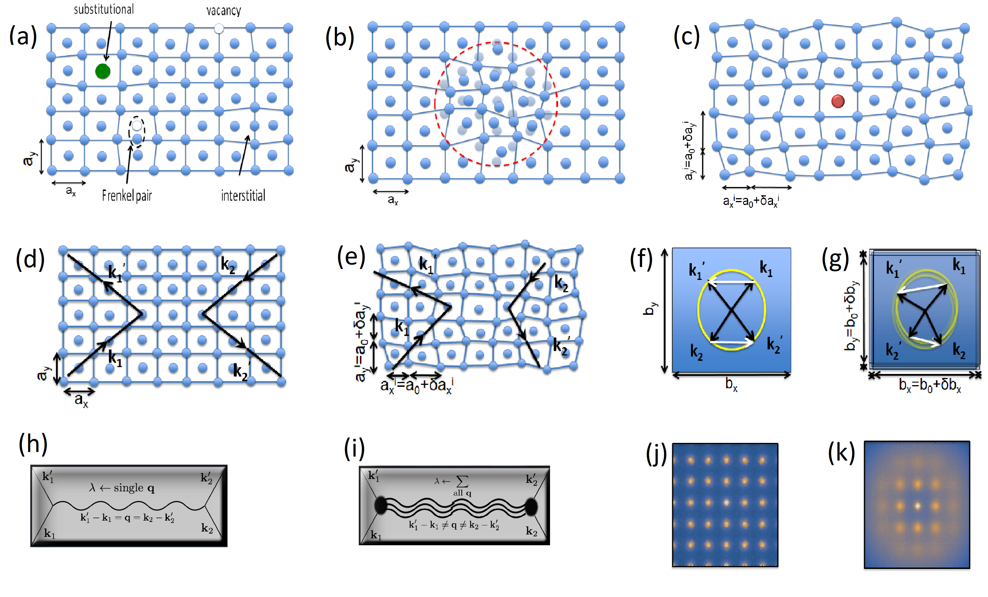
Figure 1: (a) Point defects in a crystalline solid; (b) agglomerated defects inside a spherical region, limited by a red dashed radius, $nm\ll D\ll\mu m$, and labelled as a defectal; (c) model of a defectal in terms of a distorted lattice plus a heavy scatterer. Effective two-electron scattering process occurring on the lattice, (d-e), in the first Brillouin zone, (f-g), and in terms of Feynman diagrams, (h-i). The Fraunhoffer diffraction pattern for pristine (j) and distorted (k) structures, in which a typical amorphization halo is observed at higher-order reciprocal lattice points.

II Defectals: description and implications

Analysis of the properties of defect-bearing samples reveals that only a certain type of stabilized agglomerate of defects Stritzker (1979) is capable of producing those ubiquitous, though exotic, defect-related correlations between $\rho_{\circ},T_{c}$, and $A$. For the identification of that specific type of defect agglomerate, see Fig. 1(b), let us revisit our working example of Al film. Upon either implantation, irradiation, or co-deposition, large granular regions, containing oxygen-induced agglomerated disturbances, are observed in the host material. Although these three defect-incorporating processes are quite different in their experimental setups, and in the mechanism behind defects formation, distribution in size, and arrangement, they all manifest, nevertheless, similar influences on the normal and superconducting properties of the target material, as it was empirically demonstrated for the case of oxygen implanted/co-deposited Al thin films Sinnecker et al. (2017).

We envisage that an implanted/co-deposited oxygen acts as an active anchor that leads to the creation and/or stabilization of large amorphized disturbances. Each separate agglomerate can be thought of as a three-dimensional disordered metallic granule embedded in an otherwise perfectly arranged metallic host, Fig. 1(b). Each of these 3-d agglomerate of defects within which an effective electron-electron scattering channel can be opened is labeled as a defectal and sketched in Fig. 1(b).

Inasmuch the same way as with our working example of oxygen implanted/irradiated/co-deposited Al thin films, defectals can also be engineered in most simple metals or metallic alloys through any disordering technique (e.g. quenched condensation, cold working, alloying, electron irradiation, etc) provided some sort of stabilizing anchor such O, H, etc, is present. Before entering into the details of our theoretical formulation for the consequences of defectal incorporation in conventional superconductors, let us revise some empirical curves depicting the evolution of $T_{c}(\rho_{\circ})$ and $A(\rho_{\circ})$ for a variety of systems.

II.1 Correlation $T_{c}\times\rho_{\circ}$

Figure 2 shows the evolution of $\frac{T_{c}-T^{\circ}_{c}}{T^{\circ}_{c}}~{}vs~{}\frac{\rho_{\circ}-\rho^{\circ}_{\circ}}{\rho^{\circ}_{\circ}}$ for a variety of defectal-incorporated materials. Here, $\rho^{\circ}_{\circ}$ and $T^{\circ}_{c}$ are the initial values of the residual resistivity and superconducting transition temperature, respectively, before the intentional addition of defectals. As such, $\delta\rho_{\circ}\equiv\rho_{\circ}-\rho^{\circ}_{\circ}$ is a measure of the amount of the intentionally-introduced defectals. In spite of the extensive list of differing materials and/or disordering techniques, the evolution of $\frac{\delta T_{c}}{T^{\circ}_{c}}~{}vs~{}\frac{\delta\rho_{\circ}}{\rho^{\circ}_{\circ}}$ can be classified into two distinct categories, discussed below.

II.1.1 Weakly-coupled superconductors

Figs. 2(b-c), shows the cases of In Heim et al. (1978); Bergmann (1969); Bauriedl et al. (1976); Hofmann et al. (1981); Miehle et al. (1992), Zn Miehle et al. (1992), Ga Miehle et al. (1992); Görlach et al. (1982), Al₂Au Miehle et al. (1992), AuIn₂ Miehle et al. (1992), Sn Bergmann (1969), and Al Miehle et al. (1992); Ziemann et al. (1979). Various other weakly-coupled superconductors (e.g. simple metals Be, Zn, Cd) Ochmann and Stritzker (1983) can be added to this list. A common property is that defectal incorporation leads to an enhancement of $T_{c}$ and $\rho_{\circ}$, linear for small $\delta\rho_{\circ}$, $\delta T_{c}\propto\delta\rho_{\circ}$, with a slope that depends solely on material properties (see the thick red line in Figs. 2(b-c)). It is worth noting that the manifestation of such correlation in self-ion irradiation of aluminum film, Fig. 2(c), indicates that defectal formation and stabilization does not depend on the chemical character of the bombarding projectiles (provided there is oxygen as a stabilizing anchor).

II.1.2 Strongly-coupled superconductors

Fig. 2(h-i), shows the cases of V₃Si Meyer (1980, 1980), Nb Linker (1980); Heim and Kay (1975); Linker (1980), Nb3Ge Testardi et al. (1977), V3Si Testardi and Mattheiss (1978); Meyer (1980), V3Ge Testardi et al. (1977), Pb Miehle et al. (1992), and Pb_1-xGe_x (x=0.3, 0.7) Zawislak et al. (1981). In this class, defectal incorporation leads to a reduction in $T_{c}$ together with an increase in $\rho_{\circ}$. Although Pd is a non-superconducting metal in the pure state, its hyrdogenation Stritzker and Becker (1975); Stritzker (1978, 1979), or that of its solid-solution Pd-X (X=noble metal) Stritzker (1974), leads to a superconducting state with a relatively high $T_{c}$. A common property of this class is the continuous nonlinear dependence of $\delta T_{c}$ on $\delta\rho_{\circ}$, for all $\delta\rho_{\circ}\geq 0$, and a negative derivative, $d(\delta T_{c})/d(\delta\rho_{\circ})<0$, for a majority of its members. Finally, the parabolic-like behaviour observed in Fig. 2(h) is a characteristic feature of a superconducting binary alloy, e.g. $A_{1-x}B_{x}$, wherein the residual resistivity is non-monotonic and follows Nordheim’s rule $\rho_{\circ}(x)\propto x(1-x)$.

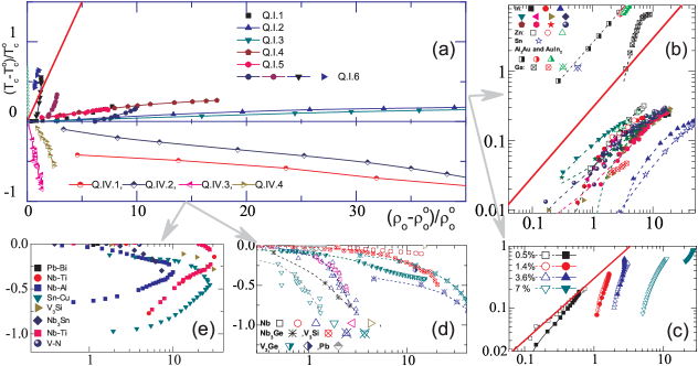
Figure 2: (a) Evolution of $\frac{\delta T_{c}}{T_{c}^{\circ}}\,~{}vs~{}\,\frac{\delta\rho_{\circ}}{\rho_{\circ}^{\circ}}$ for various defectal-bearing superconductors. Weak-coupled: Q.I.1: Al and O co-deposition Ziemann et al. (1978), Q.I.2: Indium-granular film Bergmann (1969), Q.I.3: Sn - granular Bergmann (1969), Q.I.4: In - Ar-irradiated Hofmann et al. (1981), Q.I.5: In - Ar-implanted Hofmann et al. (1981), Q.I.6: O-incorporated Al with Al-irradiation Ziemann et al. (1979). Strong-coupled: Q.IV.1: V₃Si Kr-irradiated Meyer (1980), Q.IV.2: V₃Si He-irradiated Meyer (1980), Q.IV.3: Nb N-implantated Linker (1980), Q.IV.4: Nb Ne-irradiated Linker (1980). (b) Log-log plots of irradiated/implanted thin-films of weakly-coupled conventional BCS superconductors: In Heim et al. (1978); Bergmann (1969); Bauriedl et al. (1976); Hofmann et al. (1981); Miehle et al. (1992), Zn Miehle et al. (1992), Ga Miehle et al. (1992); Görlach et al. (1982), Al2Au Miehle et al. (1992), AuIn2 Miehle et al. (1992), and Sn Bergmann (1969). (c) log-log plots of self-ion irradiation of pure (empty symbols) and granular (filled symbols) thin-films of aluminum with varying concentration of defectal-stablizing oxygen ($\leq 7\%$) Miehle et al. (1992); Ziemann et al. (1979). (d) Semi-log plots of the strong-coupled conventional BCS superconductors: Nb Heim and Kay (1975); Linker (1980), Nb3Ge Testardi et al. (1977), V3Si Testardi and Mattheiss (1978); Meyer (1980), V3Ge Testardi et al. (1977), Pb Miehle et al. (1992), and Pb_1-xGe_x (x=0.3,0.7) Zawislak et al. (1981). (e) Semi-log plot of irradiated/implanted thin-films of strong-coupled conventional BCS superconductors: Gurvitch (1986). For more details, see text.

II.2 Correlation $A\times\rho_{\circ}$

Figure 3 shows the defectal-induced evolution of $T_{c}$, $A$ and $\rho_{\circ}$ for selected representatives from each of the aforementioned two classes: the incorporation of defectals leads to the surge of $AT^{2}$ Fermi-liquid contribution, with $A$ being strongly correlated to $\rho_{\circ}$. It is remarkable that Gurvitch Gurvitch (1986) had already identified the importance of disorder-driven breakdown of momentum conservation in shaping $T_{c}$, $A$ and $\rho_{\circ}$ of superconducting alloys. Unfortunately, with the exception of that work Gurvitch (1986), such a correlation had not been highly appreciated. As such, there are no extensive reports from which one can construct a universal $\frac{A-A_{\circ}}{A_{\circ}}~{}vs~{}\frac{\rho_{\circ}-\rho^{\circ}_{\circ}}{\rho^{\circ}_{\circ}}$ plot. Nevertheless, a common, parabolic-like dependence of $A$ on $\rho_{\circ}$, like $A(\rho_{\circ})=A_{\circ}+A_{1}\rho_{\circ}+A_{2}\rho_{\circ}^{2}$, can be readily identified when examining the evolution of $A$ in the representatives of: (i) the strongly-coupled [Fig. 3(a.8)]; and (ii) the weakly-coupled [Fig. 3(b.1)] superconductors.

II.3 Correlation $T_{c}\times A$

Figure 3 also reveals a remarkable universal correlation between $T_{c}$ and $A$, with a BCS-like form, $T_{c}=\theta e^{-F/\sqrt{A}}$, wherein $\theta$ and $F$ are material-dependent parameters, specific for each superconductor. This remarkable correlation has previously been recognized and theoretically approached in a few material systems (see, e.g., the seminal, pioneering works of refs. Gurvitch (1986); Nunez-Regueiro et al. (2012); van der Marel et al. (2011); Castro et al. (2018)), but here we show that it can be unambigously traced back to the presence of defectals, being the main factor behind the establishment of such universal kinematic correlation between $T_{c}(\rho_{\circ})$ and $A(\rho_{\circ})$, and allowing us to construct a single $T_{c}~{}vs~{}\sqrt{A}$ plot [Figs. 3(a.10,b.3,c.6 and d.6) and  3] that includes many representatives of each of the two classes described above.

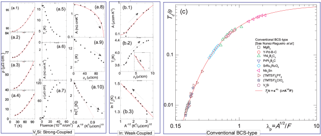
Figure 3: (a) Bulk single-crystal V3Si subjected to irradiation by neutron flux [data taken from Ref.Caton and Viswanathan, 1982]. $\rho_{\circ}(T)$ with fluences (a.1) $21.5\times 10^{18}n/cm^{2}$, (a.2) $18\times 10^{18}n/cm^{2}$, (a.3) $11\times 10^{18}n/cm^{2}$, and (a.4) $0\times 10^{18}n/cm^{2}$. The red lines are fit to $\rho_{tot}(T)=\rho_{\circ}+\beta T^{5}+AT^{2}$. (a.5) $T_{c}$   vs   fluence, (a.6) $A$   vs   fluence, and (a.7) $\rho_{\circ}$   vs   fluence. (a.8) $A$   vs   $\rho_{\circ}$, (a.9) $T_{c}$   vs   $\rho_{\circ}$, and (a.10) $ln(T_{c})$   vs   $A^{-\frac{1}{2}}$; (b) thin films of In deposited at 200K and annealed at 300K; afterwards implantated with In⁺ ions at 2K [data taken from Ref.Heim et al., 1978]: (b.1) $A$   vs   $\rho_{\circ}$, (b.2) $T_{c}$   vs   $\rho_{\circ}$, Inset: $lnT_{c}$   vs   $\rho_{\text{o}}^{\text{-1}}$, and (b.3) $ln(T_{c})$   vs   $A^{-\frac{1}{2}}$. (c) Universal kinematic correlation between $T_{c}$ and $A$ for several weakly- and strongly- coupled BCS superconductors [data taken from Ref.Nunez-Regueiro et al., 2012].

III The mechanism: distortion and softening

Generally speaking, defectal incorporation is expected to lead to significant changes to the host lattice. Figure 1(b) represents the authors’ impression of a defectal, which shall henceforth be modeled in terms of a distorted lattice plus a heavy scatterer, see Fig. 1(c). Albeit its simplicity, this model embodies the two most important outcomes following defectal incorporation: distortion and softening. The breakdown of translational invariance, and the consequent triggering of multiply-polarized, phonon-mediated, electron-electron interaction channels, as illustrated in Figs. 1(e, g, i), follows from distortion. In addition, the softening of the vibrational spectrum, and the consequent transfer of spectral weight to lower frequencies, follows from the development of low energy resonances at the lower edge of the spectrum, or quasi-localized phonon modes Lifshitz and Kosevich (1966); Gor’kov (2017), that originate from the scattering of phonon waves off heavy scatterers. As we shall soon demonstrate, these effects will determine the evolution of both superconductivity and normal-state transport.

III.1 Distortion - Hosemann’s paracrystal

Let us first introduce the concept of a distorted lattice, or a Hosemann’s paracrystal Hosemann et al. (1981). Consider, for simplicity, the defectal-free structure to be a cubic lattice with primitive unit-cell vectors $|{\bf a}_{i=1,2,3}|=a_{\circ}$. We model the defectal-bearing structure as a distorted lattice wherein the ”unit vectors” acquire a given statistical probability described by a Gaussian distribution in which the average $|\overline{\bf a}_{i=1,2,3}|=a_{\circ}$ corresponds to the center of the distribution, while the extent of the distortion is given by the Gaussian width $\sigma_{ij}=\overline{\Delta{a}_{j}}/\overline{{a}_{i}}$ Hosemann et al. (1981). For simplicity, we assume equal variance, $\sigma_{ij}=\sigma\delta_{ij}$, leading to the structure depicted in [Fig. 1(c)], whose ”unit-cell” vectors vary in length and direction from cell to cell, that can nevertheless be still organized in rows and columns. For long range crystal order, Bragg reflections occur at reciprocal lattice points, ${\bf g}(h,k,l)=h{\bf b}_{1}+k{\bf b}_{2}+l{\bf b}_{3}$, spanned in terms of primitive vectors ${\bf b}_{i=1,2,3}$ satisfying ${\bf a}_{i}\cdot{\bf b}_{j}=2\pi\delta_{ij}$. However, for defectal-bearing structures, the amplitude of ”Bragg reflections” is ever decreasing, while the line-width $\delta{\bf g}(h,k,l)$ at ${\bf g}(h,k,l)$ is monotonically broadening Hosemann et al. (1981). Fig. 1(k) shows the Frauhoffer broadening of diffraction patterns in distorted lattices and how these differ from those of a pristine crystal, Fig. 1(j).

Consider now the fate of quasi-momentum conservation during a scattering of an electron by a phonon: in a distorted lattice, an electron, initially at a state ${\bf k}_{1}$ that goes into a final state ${\bf k}_{1}^{\prime}$ after being scattered by a phonon with wavevector ${\bf q}$, transfers an amount of quasi-momentum ${\bf k}_{1}^{\prime}-{\bf k}_{1}-{\bf q}={\bf g}+\bf{\delta g}$. Evidently, for a defectal-free system, $\bf{\delta g}=0$, quasi-momentum is conserved exactly and ${\bf q}={\bf k}_{1}^{\prime}-{\bf k}_{1}-{\bf g}$; in contrast, for a defectal-bearing system, $\bf{\delta g}\neq 0$, quasi-momentum is no longer conserved in the sense that ${\bf q}={\bf k}_{1}^{\prime}-{\bf k}_{1}-{\bf g}-\delta{\bf g}$ becomes increasingly arbitrary, especially those with $\bf{\delta g}$ in higher Brillouin zones.

The above statement can be made mathematically precise with the aid of the electron-phonon structure factor, $S_{\bf q}({\bf k}_{1}^{\prime}-{\bf k}_{1})=|\varphi({\bf k}_{1}^{\prime}-{\bf k}_{1}-{\bf q})|^{2}$, written in terms of $\varphi({\bf k}_{1}^{\prime}-{\bf k}_{1}-{\bf q})=(1/\sqrt{N})\sum_{{\bf r}}e^{i({\bf k}_{1}^{\prime}-{\bf k}_{1}-{\bf q})\cdot{\bf r}}$, the electron-phonon interaction phase Ziman (1979), as defined for a lattice containing $N$ ions at ${\bf r}=n_{1}{\bf a}_{1}+n_{2}{\bf a}_{2}+n_{3}{\bf a}_{3}$. For a pristine lattice $S_{\bf q}({\bf k}_{1}^{\prime}-{\bf k}_{1})=\sum_{{\bf g}}\delta_{{\bf k}_{1}^{\prime}-{\bf k}_{1}-{\bf q},{\bf g}}$, for either normal, ${\bf g}=(0,0,0)$, or umklapp, ${\bf g}\neq(0,0,0)$, scatterings. As in a perfect crystal, the low temperature ion deformations are smooth and of long wavelength (small ${\bf q}$), one usually needs to retain normal events only and, as a result, only longitudinal phonon modes with a well defined polarization, $\hat{{\bf e}}({\bf q}={\bf k}_{1}^{\prime}-{\bf k}_{1})$, are excitable. In contrast, in a defectal-bearing system the electron-phonon structure factor acquires broadened features at ${\bf g}\neq 0$ because granular distortions provides a source of short wavelength (large ${\bf q}$) phase interference. Within the framework of the distorted lattice, these features are intrinsic, as one can verify by looking at the averaged structure factor calculated in appendix A

$$\overline{S}^{\ell}_{\bf q}({\bf k}_{1}^{\prime}-{\bf k}_{1})\approx\delta_{{\bf k}_{1}^{\prime}-{\bf k}_{1}-{\bf q},0}+\sum_{{\bf g}\neq 0}\frac{S_{max}({\bf g})}{1+\ell^{2}({\bf k}_{1}^{\prime}-{\bf k}_{1}-{\bf q}-{\bf g})^{2}}.$$ (2)

In the above expression, the peak amplitudes are $S_{max}({\bf g})=4/\sigma^{2}{\bf g}^{2}=a_{\circ}^{2}/\sigma^{2}\pi^{2}(h^{2}+k^{2}+l^{2})$, while $\ell\equiv|\delta{\bf g}|^{-1}=4/\sigma^{2}{\bf g}^{2}a_{\circ}=a_{\circ}/\sigma^{2}\pi^{2}(h^{2}+k^{2}+l^{2})$, is inversely proportional to the widths of its peaks, $\delta{\bf g}$ Hosemann et al. (1981), see appendix A. Since now ${\bf k}_{1}^{\prime}-{\bf k}_{1}-{\bf q}-{\bf g}\neq 0$, multiple phonon modes (longitudinal and transverse, of all polarizations $\hat{{\bf e}}({\bf q}\neq{\bf k}_{1}^{\prime}-{\bf k}_{1}-{\bf g})$) become kinematically available for mediating electron-electron interactions.

Let us consider the parameter $\ell$ as an effective ”mean-free path” which is proportional to the inverse of $\delta\rho_{\circ}$ (the increase in the residual resistivity due to scattering of electrons off the defectals)

$$\frac{\delta\rho_{\circ}}{\rho_{\circ}^{\circ}}=\frac{\ell_{\circ}}{\ell},\;\mbox{with}\;\ell_{\circ}=a_{\circ}\left(\frac{\rho_{\circ}^{am}}{\rho_{\circ}^{\circ}}-1\right),\;\mbox{for}\quad\rho_{\circ}^{am}\gg\rho_{\circ}^{\circ},$$ (3)

where $\rho_{\circ}^{\circ}$ and $\ell_{\circ}$ are the initial values, while $\rho_{\circ}^{am}$ is the residual resistivity for the amorphous case. Effectively, $\ell$ is a scaling length related to the degree of distortion in the primitive unit-cell vectors ($\sigma$) and, as such, can be used to continuously interpolate between two limits: the defectal-free case crystal ($\ell\rightarrow\infty$, $\rho_{\circ}\rightarrow\rho_{\circ}^{\circ}$) and the amorphous, neighboring defectals, regime ($\ell\rightarrow a_{\circ}$, $\rho_{\circ}\rightarrow\rho_{\circ}^{am}$).

III.2 Softening - Lifshitz’s resonance

Next we elaborate on the notion of a heavy scatterer, or a Lifshitz’s resonance Lifshitz and Kosevich (1966). Each one of such large collection of misplaced and/or implanted atoms, precipitates and/or granular amorphous phases, being part of a defectal or as individual entities, can also be seen, from the point of view of long wavelength phonon waves, as a heavy scatterer. This leads to a slowing down of long wavelength vibrations and to an important transfer of spectral weight towards the lower edge of the spectrum. If the amplitude of the incident and scattered phonon waves are $\varphi_{{\bf q},\nu}^{(i)}$ and $\varphi_{{\bf q},\nu}^{(s)}$ Lifshitz and Kosevich (1966), respectively, then these two quantities are related by

$$\varphi_{{\bf q},\nu}^{(s)}=\frac{1}{1-\varepsilon D(\omega)}\varphi_{{\bf q},\nu}^{(i)},$$ (4)

where $\varepsilon=({\cal M}-M)/M$, with ${\cal M}$ being an effective defect-related mass, and $D(\omega)$ is a function of only the frequency $\omega$. If the frequency of the driving wave lies inside the continuum of vibrations, especially at the bottom of the phonon bands, then $D(\omega)={\cal R}e[D(\omega)]+i{\cal I}m[D(\omega)]$, and a resonance is found at a frequency $\omega_{R}$ given by the condition $\varepsilon{\cal R}e[D(\omega_{R})]=1$. Generally, the function ${\cal R}e[D(\omega)]\sim\omega^{2}$ and the effective mass ${\cal M}$ is much heavier than the typical mass of the lattice ion, $M$. Then, for sufficiently large $\varepsilon\gg 1$, the resonance frequency ($\omega_{R}\sim 1/\sqrt{\varepsilon}$) will be located at the low-frequency range of the spectrum Lifshitz and Kosevich (1966).

The phase shift due to the phonon-wave scattering off defectals can be written as Lifshitz and Kosevich (1966)

$$\Phi(\omega)=\arctan{\left[\frac{\varepsilon{\cal I}m[D(\omega)]}{1-\varepsilon{\cal R}e[D(\omega)]}\right]},$$ (5)

which, when close to $\omega_{R}$, changes rapidly from $0$ to $\pi$, indicating that the effective impurity oscillates out of phase with respect to the underlying lattice ions. This acts as a driving force that produces the sharp resonance peak in the vibrational density of states ${\cal F}(\omega)$. For a concentration $n_{d}$ of defectals this peak is given by

$$\delta{\cal F}_{R}(\omega)=\frac{3}{\pi}\frac{d\Phi}{d\omega}\approx\frac{n_{d}}{2\pi}\frac{\Gamma}{(\omega-\omega_{R})^{2}+\frac{1}{4}\Gamma^{2}},$$ (6)

and the width $\Gamma$ of the resonance at $\omega_{R}$ is given in terms of the phase shift, $\Phi(\omega)$, during the scattering of phonon waves off a dilute concentration, $n_{d}$, as

$$\Gamma=\frac{2\pi{\cal F}(\omega_{R})}{\left\{d\Phi(\omega)/d\omega\right\}_{\omega_{R}}}.$$ (7)

As we can see, the larger the mass ${\cal M}$, the lower the frequency $\omega_{R}$, since $\omega_{R}\sim 1/\sqrt{\varepsilon}$, and the sharper the resonance will be, as $\Gamma$ is proportional to ${\cal F}(\omega_{R})$ Lifshitz and Kosevich (1966).

III.3 Combining distortions and softening

The combination of a broadened structure factor in the electron-phonon coupling and the existence of quasi-localized phonon modes lead to a generalized form for Eliashberg’s spectral function which has been calculated in appendix B

$$\alpha^{2}\mathcal{F}_{\ell}\left(\omega\right)=\sum_{\left\{\mathbf{k}^{\prime},\mathbf{k}\right\}={\bf k}_{F},\mathbf{q},\nu}\overline{S}^{\ell}_{\mathbf{q}}\left(\mathbf{k}^{\prime}-\mathbf{k}\right)\left|g_{\mathbf{k}^{\prime},\mathbf{k},\mathbf{q},\nu}\right|^{2}\left\{\delta\left(\omega-\omega_{\mathbf{q},\nu}\right)+n_{d}(\ell)\frac{2}{\pi}\frac{\Gamma}{4(\omega-\omega_{R})^{2}+\Gamma^{2}}\right\},$$ (8)

where $g_{\mathbf{k}^{\prime},\mathbf{k},\mathbf{q},\nu}=\alpha(\omega_{{\bf q},\nu})\hat{{\bf e}}({\bf q},\nu)\cdot\left({\bf k}^{\prime}-{\bf k}\right)$ is the amplitude of the electron-phonon matrix element [including the bare $\alpha(\omega_{{\bf q},\nu})$ due to all branches, $\nu=L,T_{1},T_{2}$, with dispersion $\omega_{\mathbf{q},\nu}$ and polarization $\hat{{\bf e}}({\bf q},\nu)$, see appendix A], while $\omega_{R}$ and $\Gamma$ are, respectively, the frequency and linewidth of the low-energy, quasi-localized phonon resonances associated with a density, $n_{d}(\ell)$, of Lifshitz heavy scatters.

$\alpha^{2}\mathcal{F}_{\ell}\left(\omega\right)$ of Eq.(8) summarizes, mathematically, our simple (distorted-lattice-plus-heavy-scatterer) defectal-model, as it includes: (i) the softening of the vibrational spectrum, through the continuous transfer of spectral weight, tracked by $\ell$, from high, Debye’s, to low, $\omega_{R}$, frequencies; (ii) the inclusion of new phonon branches, $\nu$, and polarizations, $\hat{{\bf e}}({\bf q},\nu)$, through $\sum_{{\bf q},\nu}$; (iii) the sum of all kinematically unconstrained wave-vectors, $\mathbf{k}^{\prime},\mathbf{k},\mathbf{g},\mathbf{q}$ ($0\leq|{\bf q}|\leq 2k_{F}$) whose rules of momentum transfer are controlled by $\overline{S}^{\ell}_{\mathbf{q}}\left(\mathbf{k}^{\prime}-\mathbf{k}\right)$. We calculated $\alpha^{2}\mathcal{F}_{\ell}\left(\omega\right)$ of Eq.(8) within the Debye model for phonons interacting with nearly-free electrons, see appendix B: its evolution for different values of $\ell$, is shown in Fig. 5(g).

IV Superconductivity and FL transport

After incorporating distortion and softening, let us consider the two-particle process, shown in Figs. 1(e, g, i), wherein electrons, initially at states ${\bf k}_{1}$ and ${\bf k}_{2}$, scatter into final states ${\bf k}_{1}^{\prime}$ and ${\bf k}_{2}^{\prime}$ by the exchange of all kinematically unconstrained phonon modes ${\bf q}$ with a nonzero spectral weight. The resulting retarded, attractive electron-electron interaction reads

$$V_{{\bf k}_{1}^{\prime},{\bf k}_{1},{\bf k}_{2}^{\prime},{\bf k}_{2}}({\bf q},\ell)\approx-\phi_{{\bf q}}({\bf k}_{1}^{\prime},{\bf k}_{1},{\bf k}_{2}^{\prime},{\bf k}_{2})V_{ee}(\ell),$$ (9)

and fully expounds the roles of distortions and softening through its phase, $\phi_{{\bf q}}({\bf k}_{1}^{\prime},{\bf k}_{1},{\bf k}_{2}^{\prime},{\bf k}_{2})=(1/N)\sum_{{\bf r}}e^{i({\bf k}_{1}^{\prime}-{\bf k}_{1}-{\bf q})\cdot{\bf r}}\sum_{{\bf r}^{\prime}}e^{i({\bf k}_{2}^{\prime}-{\bf k}_{2}+{\bf q})\cdot{\bf r}^{\prime}}$, and amplitude, $V_{ee}(\ell)$, obtained after averaging over Fermi and Debye surfaces. Now let us consider the influence of distortions and softening on $T_{c}(\ell)$, $A(\ell)$, and their correlations.

IV.1 $T_{c}(\ell)$ from Eliashberg’s theory

$T_{c}(\ell)$ will be calculated as the zero gap limit, $\Delta_{\ell}\rightarrow 0$, of the system of Eliashberg’s equations in imaginary time ($i\omega_{n}=i\pi T(2n-1)$)

$$\Delta_{\ell}(i\omega_{n})Z_{\ell}(i\omega_{n}) = \pi T\sum_{m}\left[\lambda_{\ell}(i\omega_{m}-i\omega_{n})-\mu^{*}(\omega_{c})\theta(\omega_{c}-|\omega_{m}|)\right]\frac{\Delta_{\ell}(i\omega_{m})}{\sqrt{\omega_{m}^{2}+\Delta_{\ell}^{2}(i\omega_{m})}},$$

$$Z_{\ell}(i\omega_{n}) = 1+\frac{\pi T}{\omega_{n}}\sum_{m}\lambda_{\ell}(i\omega_{m}-i\omega_{n})\frac{\omega_{m}}{\sqrt{\omega_{m}^{2}+\Delta_{\ell}^{2}(i\omega_{m})}},$$ (10)

where the Coulomb pseudo-potential

$$\mu^{*}(\omega_{c})=\frac{\mu}{1+\mu\ln{\left(\frac{\epsilon_{F}}{\omega_{c}}\right)}},$$ (11)

is given in terms of the bare, repulsive Coulomb interaction, $\mu=N(\epsilon_{F})V_{C}$, and the cutoff frequency $\omega_{c}$, while $\lambda_{\ell}$ is the distortion-influenced electron phonon coupling

$$\lambda_{\ell}(i\omega_{m}-i\omega_{n}) = 2\int_{0}^{\infty}\frac{\omega\;\alpha^{2}{\cal{F}_{\ell}}(\omega)}{(\omega_{m}-\omega_{n})^{2}+\omega^{2}}d\omega$$ (12)

$$\equiv N(\epsilon_{F})V_{ee}(i\omega_{m}-i\omega_{n};\ell),$$

wherein $V_{ee}(i\omega_{m}-i\omega_{n};\ell)$ is the retarded, attractive, effective electron-electron interaction in a distorted lattice, mediated by phonons. As usual, $N(\epsilon_{F})$ is the electronic density of states at the Fermi level.

Following Allen and Dynes Allen and Dynes (1975) we introduce a two-square-well model

$$\lambda_{\ell}(i\omega_{m}-i\omega_{n})=\begin{cases}\lambda_{\ell}&\mbox{for}\quad|\omega_{m}|,|\omega_{n}|\ll\omega_{c},\\ 0&otherwise\end{cases}$$ (13)

with the coupling strength given by

$$\lambda_{\ell}=2\int_{0}^{\infty}\frac{\omega\;\alpha^{2}{\cal{F}_{\ell}}(\omega)}{\omega_{opt}^{2}+\omega^{2}}d\omega\equiv N(\epsilon_{F})V_{ee}(\ell),$$ (14)

where $\omega_{opt}$ is an optimal frequency at which $\lambda_{\ell}$ is maximal. Some comments are in order. The traditional choice for the electron-phonon coupling in the two-square-well approximation is $\lambda(i\omega_{m}-i\omega_{n})=\lambda(0)=\lambda$, where the Matsubara sums are performed, while maintaining $\omega_{m}=\omega_{n}$ at all times. This choice of an instantaneous interaction works well for weakly-coupled superconductors, which are characterized by a vibrational spectrum heavily weighted at high frequencies in such a way that the characteristic phonon frequency, $\langle\omega\rangle_{\alpha^{2}{\cal F}}$, corresponding to an average over the material’s vibrational spectral function, is always much higher than any possible difference $|\omega_{m}-\omega_{n}|=2\pi|m-n|k_{B}T/\hslash\ll\omega_{c}$. As spectral weight is transferred towards lower frequencies, however, retardation demands that we allow for $m\neq n$ in the Matsubara sums. One could choose $m-n=1$, which would result in $\omega_{opt}=2\pi k_{B}T_{c}/\hslash$, at the transition temperature, or one could use Carbotte’s argument for an estimate of the optimal frequency Carbotte (1990): Consider a harmonic oscillator of frequency $\omega$, wherein the polarization is maximal around $\omega\approx\omega_{opt}$. The oscillator is then set to oscillate by a passing electron with Fermi velocity $v_{F}$. If the lattice oscillates too slowly, $\omega\ll\omega_{opt}$, there will be no polarization effects, within a region of the size of the coherence length, $\xi_{0}$, on a second passing electron with the same velocity $v_{F}$; if it oscillates too rapidly, $\omega\gg\omega_{opt}$, the polarization will average out to zero before the second electron has left the coherence perimeter. Either way, the retarded interaction must vanish at both $\omega\rightarrow 0$ and $\omega\rightarrow\infty$ and be maximal at $\omega_{opt}$, which in terms of $v_{F}$ and $\xi_{0}$ can then be written as $\omega_{opt}=\pi v_{F}/2\xi_{0}$. Alternatively, $\omega_{opt}$ has been estimated, after inclusion of various Matsubara frequencies, all satisfying $|\omega_{m}|,|\omega_{n}|\ll\omega_{c}$, to be roughly $\omega_{opt}\approx 10k_{B}T^{max}_{c}/\hslash$ (slightly higher than the lowest bound of $2\pi k_{B}T_{c}/\hslash$ for $m-n=1$ discussed before) where $T^{max}_{c}$ is the maximum possible value for $T_{c}$ in the defectal-free system. All in all, the presence of an optimal frequency, $\omega_{opt}\neq 0$, implies that our retarded, effective $V_{ee}(\ell)$ is most effective around $\omega_{opt}$, while drops to zero at both $\omega\rightarrow\infty$ and $\omega\rightarrow 0$ limits: as also shown in Fig. 5(h).

Using the above notation, $Z_{\ell}=1+\lambda_{\ell}$ and the zero gap limit, $\Delta_{\ell}\rightarrow 0$, of Eliashberg’s equations reduces to

$$1=\frac{\lambda_{\ell}-\mu^{*}}{1+\lambda_{\ell}}\pi T_{c}\sum_{|\omega_{m}|<\omega_{c}}\frac{1}{|\omega_{m}|}\simeq\frac{\lambda_{\ell}-\mu^{*}}{1+\lambda_{\ell}}\ln{\left[\frac{2e^{\gamma}\omega_{c}}{\pi T_{c}}\right]},$$ (15)

where $\gamma\simeq 0.577$ is Euler’s constant. Now we can exponentiate both sides to arrive at the usual MacMillan McMillan (1968) (or simplified Allen-Dynes Allen and Dynes (1975)) result for $T_{c}$

$$T_{c}(\ell)=\theta e^{-(1+\lambda_{\ell})/(\lambda_{\ell}-\mu^{*})}\quad\mbox{with}\quad\theta=\frac{1.13\hbar\omega_{c}}{k_{B}}.$$ (16)

The calculation of $T_{c}(\ell)$ depends on the strength of the electron-phonon coupling $\lambda_{\ell}$ which, in turn, is determined by the amplitude, $V_{ee}(\ell)$, via eq. (14). As we can see, $\lambda_{\ell}$ is highly sensitive to softening, namely, to shifts in spectral weight relative to an optimal frequency $\omega_{opt}$. According to the scaling theorem of Coombes and Carbotte Carbotte (1990), when the total integrated area under the spectral function, $\alpha^{2}\mathcal{F}_{\ell}\left(\omega\right)$ in Eq.(8), is equal to a constant $\mathcal{A}$, then the best shape that maximizes $T_{c}$ is a $\delta$-function which, here, is introduced as an Einstein spectrum

$$\alpha^{2}\mathcal{F}_{\ell}\left(\omega\right) = \mathcal{A}\delta\left(\omega-\omega_{E}(\ell)\right),$$

$$\omega_{E}(\ell) \approx \left(1-\frac{1}{k_{F}\ell}\right)\omega_{E}(\infty)+\frac{1}{k_{F}\ell}\omega_{R},\quad\mbox{for }k_{F}\ell\gg 1,$$ (17)

wherein the material dependent $\omega_{E}(\infty)$ is an average phonon frequency calculated self-consistently in terms of the defectal-free $\alpha^{2}\mathcal{F}_{\infty}\left(\omega\right)$; $\omega_{E}(\ell)$ is a monotonically decreasing function of $\ell$, valid for $k_{F}\ell\gg 1$ as $\ell$ is decreased towards $a_{\circ}$: such a softening is manifested in all materials undergoing amorphization Bergmann (1976). The evolution of the normalized $\lambda_{\ell}$ undergoing such a softening is

$$\frac{\delta\lambda_{\ell}}{\lambda_{\infty}} \equiv \frac{\lambda_{\ell}-\lambda_{\infty}}{\lambda_{\infty}}$$ (18)

$$= \frac{1}{k_{F}\ell}\left[\frac{\omega_{E}^{2}(\infty)}{\omega_{opt}^{2}+\omega_{E}^{2}(\infty)}\left(2-\frac{1}{2k_{F}\ell}\right)-1\right]+{\cal O}\left(\frac{1}{\ell^{3}}\right).$$

wherein both $\omega_{E}(\ell)$ and $\omega_{opt}$ are much higher than the resonance frequency $\omega_{R}$, see Fig. 5(g)-(h). The associated evolution of $T_{c}(\ell)$ is shown in Fig. 4(a) for the two classes of conventional superconductors discussed below.

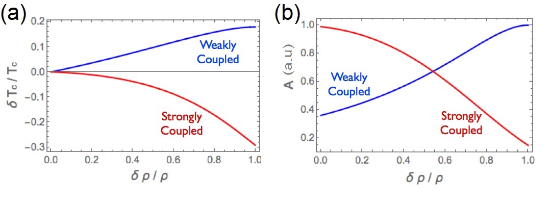
Figure 4: Correlated variations of $\delta T_{c}(\delta\rho_{\circ}/\rho_{\circ})/T_{c}$ (left, (a)) and $A(\delta\rho_{\circ}/\rho_{\circ})$ (right, (b)), for the two classes of conventional superconductors considered in this work: weakly-coupled superconductors (red, decreasing) and strongly-coupled superconductors (blue, increasing).

IV.1.1 Weakly coupled superconductors

A defectal-free member of this class is characterized by $\omega_{E}(\infty)\gg\omega_{opt},\omega_{R}$: then $\lambda_{\infty}\ll 1$ and $T_{c}$ is low. Incorporation of defectals leads to $\delta\rho_{\circ}\equiv(\partial\rho_{\circ}/\partial\ell)\delta\ell>0$ (since $\delta\ell<0$) and, based on Eq.(17), a shift in $\omega_{E}(\ell)$ towards $\omega_{opt}$. From the structure of $V_{ee}\left(\omega_{E}/\omega_{opt}\right)$, shown in Fig. 5(g), one concludes that weakly-coupled superconductors exhibit an enhancement of both $\lambda_{\ell}$ and $T_{c}(\ell)$ upon defectal incorporation. Furthermore, recalling that $\omega_{E}(\ell)\gg\omega_{opt},\omega_{R}$, for $1\ll k_{F}\ell<\infty$, and $\ell/\ell_{\circ}=\rho_{\circ}^{\circ}/\delta\rho_{\circ}$, one arrives at [see Eq.(18, 16)]

$$\frac{\delta T_{c}(\delta\rho_{\circ}/\rho_{\circ}^{\circ})}{T_{c}^{\circ}}\approx\frac{\lambda_{\infty}}{(\lambda_{\infty}-\mu^{*})^{2}}\frac{1}{k_{F}\ell_{\circ}}\left(\frac{\delta\rho_{\circ}}{\rho_{\circ}^{\circ}}\right),$$ (19)

for weak but positive $\frac{\delta\rho_{\circ}}{\rho_{\circ}^{\circ}}$, a linear evolution universally valid within the weak defectal-concentration range: consistent with the empirical analysis provided earlier for superconductors belonging to the upper quadrant of Fig. 2, and with a slope determined solely by material properties such as $k_{F}\ell_{\circ}$, $\lambda_{\infty}$, and $\mu^{*}$, see Fig. 4(a)(blue).

IV.1.2 Strongly-coupled superconductors

Here a defectal-free member is characterized by $\omega_{E}(\infty)\lessapprox\omega_{opt}$ and $\omega_{E}(\infty)\gg\omega_{R}$; accordingly $\lambda_{\infty}\sim 1$ and relatively high $T_{c}$. Incorporation of defectals in such systems increases $\delta\rho_{\circ}>0$ and a shift in $\omega_{E}(\ell)$, away from $\omega_{opt}$ but towards $\omega_{R}$. From the structure of $V_{ee}\left(\omega_{E}/\omega_{opt}\right)$, shown in Fig. 5(g), one concludes that strongly-coupled superconductors exhibit a reduction of both $\lambda_{\ell}$ and $T_{c}(\ell)$ upon defectal incorporation. It is recalled that $\omega_{E}(\ell)\lessapprox\omega_{opt}$ and $\lambda_{\infty}\gg\mu^{*}$ for $1\ll k_{F}\ell<\infty$. Then based on Eqs.(17,18), one obtains

$$\frac{\delta T_{c}(\delta\rho_{\circ}/\rho_{\circ}^{\circ})}{T_{c}^{\circ}}\approx-t_{1}\left(\frac{\delta\rho_{\circ}}{\rho_{\circ}^{\circ}}\right)-t_{2}\left(\frac{\delta\rho_{\circ}}{\rho_{\circ}^{\circ}}\right)^{2},$$ (20)

with $t_{1}=(\lambda_{\infty}^{-1}/k_{F}\ell_{\circ})(1-2\omega_{E}^{2}(\infty)/(\omega_{opt}^{2}+\omega_{E}^{2}(\infty)))$, positive for $\omega_{E}(\infty)\lessapprox\omega_{opt}$, and a reasonably large value for $t_{2}=(\lambda_{\infty}^{-1}/8k_{F}\ell_{\circ})\omega_{E}^{2}(\infty)/(\omega_{opt}^{2}+\omega_{E}^{2}(\infty))>0$. This shows a deviation from linearity which is consistent with the empirical analysis of the lower quadrant of Fig. 2, see also Fig. 4(a)(red).

IV.2 $A(\ell)$ from Boltzmann’s transport theory

The calculation of the FL coefficient $A$ depends on the availability of momentum relaxation channels associated with the two-particle process within a defectal-bearing lattice; such an availability is determined by the amount of distortion which directly affects the phase, $\phi_{{\bf q}}$, via

$$f_{\ell}({\bf k}_{1}^{\prime},{\bf k}_{1},{\bf k}_{2}^{\prime},{\bf k}_{2})=\sum_{\bf q}\overline{S}^{\ell}_{{\bf q}}({\bf k}_{1}^{\prime}-{\bf k}_{1})\overline{S}^{\ell}_{-{\bf q}}({\bf k}_{2}^{\prime}-{\bf k}_{2}),$$ (21)

with the quasi-momentum transfer being controlled by a convolution between two $\overline{S}^{\ell}_{{\bf q}}({\bf k}_{i}^{\prime}-{\bf k}_{i})$ factors. The Fermi liquid coefficient, $A(\ell)$, of a distorted lattice will be calculated from the electron-electron scattering including both the direct Coulomb $V_{C}$ and the retarded, effective (phonon-mediated) electron-electron interaction $V_{ee}(\ell)$. We will look for a variational solution, $\Phi_{{\bf k}}$, to the linearized Boltzmann’s transport equations in terms of which the resistivity can be written as Ziman (1979)

$$\rho_{ee}(T,\ell)=\frac{\langle\Phi_{{\bf k}},{\cal P}_{\ell}\Phi_{{\bf k}}\rangle}{\left|\langle\Phi_{{\bf k}},X\rangle\right|^{2}}=A(\ell)T^{2},$$ (22)

where ${\cal P}_{\ell}$ is the scattering operator that transforms the variational solution $\Phi_{{\bf k}}$ into another momentum state, ${\bf k}^{\prime}$. Through integration, the normalization factor reads

$$\left|\langle\Phi_{{\bf k}},X\rangle\right|=\left|2e\sum_{{\bf k}}v_{{\bf k}}\Phi_{{\bf k}}\left(-\frac{\partial f\left(\epsilon_{{\bf k}}\right)}{\partial\epsilon_{{\bf k}}}\right)\right|=\frac{ek_{F}^{3}}{3\pi^{2}\hbar m^{*}}=\frac{ne}{m^{*}},$$ (23)

with $\Phi_{{\bf k}}=\vec{u}\cdot\vec{{\bf v}}_{{\bf k}}$ measuring the deviation of the electronic distribution from equilibrium, $\vec{u}$ being the direction of the applied electric field, and $\vec{{\bf v}}_{{\bf k}}$ the velocity of the quasiparticle associated with momentum ${\bf k}$. In terms of these quantities, the numerator reads Ziman (1979)

$$\langle\Phi_{{\bf k}},{\cal P}_{\ell}\Phi_{{\bf k}}\rangle=\frac{1}{2k_{B}T} \sum_{{\bf k}_{1},{\bf k}_{2},{\bf k}_{1}^{\prime},{\bf k}_{2}^{\prime}} f_{\epsilon_{{\bf k}_{1}}}f_{\epsilon_{{\bf k}_{2}}}(1-f_{\epsilon_{{\bf k}_{1}^{\prime}}})(1-f_{\epsilon_{{\bf k}_{2}^{\prime}}})\delta(\epsilon_{{\bf k}_{1}}+\epsilon_{{\bf k}_{2}}-\epsilon_{{\bf k}_{1}^{\prime}}-\epsilon_{{\bf k}_{2}^{\prime}})$$ (24)

$$\times (\Phi_{{\bf k}_{1}}+\Phi_{{\bf k}_{2}}-\Phi_{{\bf k}_{1}^{\prime}}-\Phi_{{\bf k}_{2}^{\prime}})^{2}\Gamma_{{\bf k}_{1}+{\bf k}_{2}\rightarrow{\bf k}_{1}^{\prime}+{\bf k}_{2}^{\prime}}(\ell),$$

wherein $\Gamma_{{\bf k}_{1}+{\bf k}_{2}\rightarrow{\bf k}_{1}^{\prime}+{\bf k}_{2}^{\prime}}(\ell)$ is the transition amplitude for the total electron-electron interaction, $V_{tot}(\ell)$, while $f_{\epsilon_{{\bf k}}}$ is the equilibrium electron distribution

$$f_{\epsilon_{{\bf k}}}=\frac{1}{e^{\beta(\epsilon_{{\bf k}}-\mu)}-1},$$ (25)

with $\beta=1/k_{B}T$, $\epsilon_{F}$ the Fermi energy and $\mu=\epsilon_{F}$.

At this point it is important to emphasize that when approaching the superconducting instability from the Fermi-liquid state, $T\rightarrow T_{c}^{+}(\ell)$, the total electron-electron interaction, $V^{0}_{tot}(\ell)=V_{C}-V_{ee}(\ell)$ becomes renormalized according to

$$V^{0}_{tot}(\ell)\rightarrow V_{tot}(\ell)=\frac{V_{C}-V_{ee}(\ell)}{Z_{\ell}}=\frac{V_{C}-V_{ee}(\ell)}{1+\lambda_{\ell}},$$ (26)

where the renormalization constant, $Z_{\ell}$, is the same as obtained when approaching from the superconducting ground state, $T\rightarrow T_{c}^{-}(\ell)$. This is an asymptotically exact result obtained by using a renormalization group procedure that treats the direct and effective parts of the total interaction on equal footing Tsai et al. (2005).

At low temperatures, we can project all electron states at the Fermi surface, $|{\bf k}_{i}|=k_{F}$, and transform $\sum_{{\bf k}_{i}}$ into integrals over $\epsilon_{{\bf k}_{i}}$, with a constant electronic density of states at the Fermi level, as well as integrals over solid angles. The constraint of energy conservation can also be rewritten in terms of the transferred energy, $\hbar\omega$, to the phonons

$$\delta(\epsilon_{{\bf k}_{1}}+\epsilon_{{\bf k}_{2}}-\epsilon_{{\bf k}_{1}^{\prime}}-\epsilon_{{\bf k}_{2}^{\prime}})=\int_{-\infty}^{\infty}d\omega\;\delta(\epsilon_{{\bf k}_{1}^{\prime}}-\epsilon_{{\bf k}_{1}}-\hbar\omega)\delta(\epsilon_{{\bf k}_{2}^{\prime}}-\epsilon_{{\bf k}_{2}}+\hbar\omega),$$ (27)

which allows us to eliminate both $\epsilon_{{\bf k}_{1}^{\prime}}$ and $\epsilon_{{\bf k}_{2}^{\prime}}$, after which we are left with

$$\int d\epsilon_{{\bf k}_{1}}\int d\epsilon_{{\bf k}_{2}}\>f_{\epsilon_{{\bf k}_{1}}}f_{\epsilon_{{\bf k}_{2}}}(1-f_{\epsilon_{{\bf k}_{1}}+\hbar\omega})(1-f_{\epsilon_{{\bf k}_{2}}-\hbar\omega})=\frac{\hbar^{2}\omega^{2}}{(e^{\beta\hbar\omega}-1)(1-e^{-\beta\hbar\omega})}.$$ (28)

Finally, we can integrate over the transferred energy $\hbar\omega$ to obtain

$$\frac{1}{2k_{B}T}\int_{-\infty}^{\infty}d(\hbar\omega)\frac{\hbar^{2}\omega^{2}}{(e^{\beta\hbar\omega}-1)(1-e^{-\beta\hbar\omega})}=\frac{\pi^{2}}{3}(k_{B}T)^{2},$$ (29)

which ensures that the contribution to the resistivity from this novel electron-electron interaction has the typical Fermi liquid quadratic-in-T, $\rho_{ee}(T,\ell)=A(\ell)T^{2}$ with

$$A(\ell)=\left(\frac{m^{*}}{ne}\right)^{2}\frac{\pi^{2}k_{B}^{2}}{3(\hbar v_{F})^{4}}\int\int\int\int\frac{d\Omega_{{\bf k}_{1}}d\Omega_{{\bf k}_{1}^{\prime}}d\Omega_{{\bf k}_{2}}d\Omega_{{\bf k}_{2}}^{\prime}}{(2\pi)^{12}}(\Phi_{{\bf k}_{1}}+\Phi_{{\bf k}_{2}}-\Phi_{{\bf k}_{1}^{\prime}}-\Phi_{{\bf k}_{2}^{\prime}})^{2}\times\Gamma_{{\bf k}_{1}+{\bf k}_{2}\rightarrow{\bf k}_{1}^{\prime}+{\bf k}_{2}^{\prime}}(\ell),$$ (30)

and $\Gamma_{{\bf k}_{1}+{\bf k}_{2}\rightarrow{\bf k}_{1}^{\prime}+{\bf k}_{2}^{\prime}}(\ell)$ calculated by the use of Fermi’s golden rule

$$\Gamma_{{\bf k}_{1}+{\bf k}_{2}\rightarrow{\bf k}_{1}^{\prime}+{\bf k}_{2}^{\prime}}(\ell)=\left(\frac{2\pi}{\hbar}\right)\left|V_{tot}(\ell)\right|^{2}f_{\ell}({\bf k}_{1}+{\bf k}_{2}-{\bf k}_{1}^{\prime}-{\bf k}_{2}^{\prime}),$$ (31)

where $f_{\ell}({\bf k}_{1}+{\bf k}_{2}-{\bf k}_{1}^{\prime}-{\bf k}_{2}^{\prime})$ regulates all kinematic constraints through eq. (21). After projecting all ${\bf k}_{i}$ states onto the roughened Fermi surface, we thus obtain

$$A(\ell)=F^{2}_{\ell}\left|V_{tot}(\ell)\right|^{2},$$ (32)

where the so called efficiency of momentum relaxation

$$F^{2}_{\ell}=F^{2}_{\circ}\int\int\int\int\frac{d\Omega_{{\bf k}_{1}}\,d\Omega_{{\bf k}_{1}^{\prime}}\,d\Omega_{{\bf k}_{2}}\,d\Omega_{{\bf k}_{2}^{\prime}}}{(2\pi)^{12}}(\Phi_{{\bf k}_{1}}+\Phi_{{\bf k}_{2}}-\Phi_{{\bf k}_{1}^{\prime}}-\Phi_{{\bf k}_{2}^{\prime}})^{2}\times f_{\ell}({\bf k}_{1}+{\bf k}_{2}-{\bf k}_{1}^{\prime}-{\bf k}_{2}^{\prime}),$$ (33)

with

$$F^{2}_{\circ}=(2\pi/\hbar)(m^{*}/ne)^{2}(\pi^{2}k_{B}^{2}/3\hbar^{4}v_{F}^{4})(1/N^{2}(\epsilon_{F})),$$ (34)

where $\Phi_{{\bf k}}=\vec{u}\cdot{\bf v}_{\bf k}$, $\vec{u}$ is the unit vector along the direction of the applied electric field, ${\bf v}_{\bf k}=\hbar{\bf k}/m^{*}$ is the quasiparticle velocity of carriers having effective mass $m^{*}$.

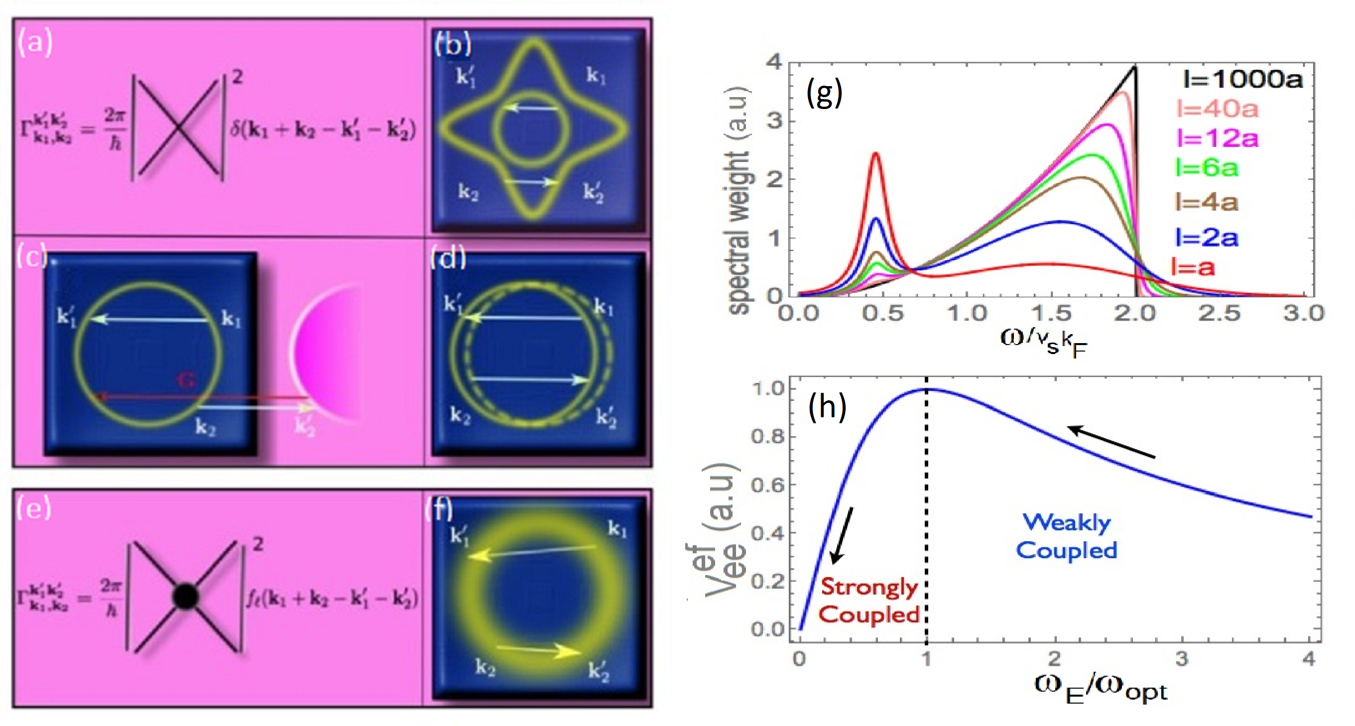
Figure 5: (a) $\Gamma_{{\bf k}_{1},{\bf k}_{2}}^{{\bf k}_{1}^{\prime},{\bf k}_{2}^{\prime}}$ of a defectal-free system with kinematically constrained relaxation channels: (b) multi-band or Baber scattering; (c) multi-zone, or Umklapp, scattering; (d) multi-sheet, or topological, scattering. (e) $\Gamma_{{\bf k}_{1},{\bf k}_{2}}^{{\bf k}_{1}^{\prime},{\bf k}_{2}^{\prime}}$, of a defectal-bearing system with kinematically unconstrained relaxation channel: (f) the novel halo-umklapp scattering mechanism; (g) Eliashberg’s spectral function, $\alpha^{2}{\cal F}$ as a funcion of $\omega/v_{s}k_{F}$ for different values of $\ell$ showing the transfer of spectral weight from high- to low- frequencies; (h) effective electron-electron, $V_{ee}$, interaction as a function of $\omega_{E}/\omega_{opt}$ showing phonon softening and the increase of the interaction for weakly-coupled superconductors, and its decrease for strong coupling.

IV.2.1 Relaxed kinematics and the robustness of the FL

The precise evaluation of $F^{2}_{\ell}$ requires a microscopic calculation that includes all possible relaxation, momentum-transferring channels such that

$$[\vec{u}\cdot({\bf k}_{1}+{\bf k}_{2}-{\bf k}_{1}^{\prime}-{\bf k}_{2}^{\prime})]^{2}\times f_{\ell}({\bf k}_{1}+{\bf k}_{2}-{\bf k}_{1}^{\prime}-{\bf k}_{2}^{\prime})\neq 0.$$ (35)

As evident, the fate of the Fermi-liquid coefficient, $A(\ell)$, for different Fermi surface topologies, will be determined essentially by the available phase space for scattering, because this enters into the integration over solid angles, $\int...d\Omega_{{\bf k}_{i}}$, with the integrand containing the product between the large angle scattering factor, equivalent to $(1-\cos\theta)$, and the scattering transition amplitude, $(\Phi_{{\bf k}_{1}}+\Phi_{{\bf k}_{2}}-\Phi_{{\bf k}_{1}^{\prime}}-\Phi_{{\bf k}_{2}^{\prime}})^{2}\times f_{\ell}({{\bf k}_{1}+{\bf k}_{2}\rightarrow{\bf k}_{1}^{\prime}+{\bf k}_{2}^{\prime}})$.

In a defectal-free system (e.g. our example of Al thin films), we have $f_{\infty}({{\bf k}_{1}+{\bf k}_{2}\rightarrow{\bf k}_{1}^{\prime}+{\bf k}_{2}^{\prime}})=\delta_{{{\bf k}_{1}+{\bf k}_{2},{\bf k}_{1}^{\prime}+{\bf k}_{2}^{\prime}}}$, and kinematics severely restricts the availability of phase space for net momentum transfer to the lattice to the following scattering channels shown in Fig. 5(b)-(d): (i) the Baber mechanism, for a multi-band Fermi surface Baber (1937); (ii) the umklapp mechanism, for Fermi surfaces that are at least quarter-filled Yamada and Yosida (1986); Maebashi and Fukuyama (1998); and (iii) the normal mechanism, for multiply connected Fermi surfaces with an infinite number of self-intersecting points Pal et al. (2012). As a result, any $A(\infty)T^{2}$ contribution allowed by these channels is typically very small, $A(\infty)\sim 10^{-7}\mu\Omega$cmK^-2 (low scattering efficiency), or even identically vanishing, $A(\infty)\equiv 0$, for topologically trivial, single band, small Fermi surface systems. The extreme specificity of the above relaxation mechanisms is in stark disagreement with the ubiquitous experimental observation of a robust Fermi liquid behavior in the transport properties of defectal-bearing superconductors (see, e.g., Fig. 3).

The stabilization of the FL behaviour clearly requires a remarkable increase in phase space for scattering as the one promoted by defectals. In this case, the kinematic constraints are relaxed due to the breakdown of translational invariance, $f_{\ell}({{\bf k}_{1}+{\bf k}_{2}\rightarrow{\bf k}_{1}^{\prime}+{\bf k}_{2}^{\prime}})\neq\delta_{{{\bf k}_{1}+{\bf k}_{2},{\bf k}_{1}^{\prime}+{\bf k}_{2}^{\prime}}}$, and a robust FL behaviour results, $A(\ell<\infty)\neq 0$, over a rather wide temperature range. We call the mechanism behind such large values for $A(\ell<\infty)\neq 0$ as halo-umklapp scattering, whereby the enlargement of the available phase space for quasi-momentum relaxation stems from the monotonically increasing broadening of the Bragg reflections at higher-order reciprocal lattice points, which eventually merge together to produce a halo-shaped diffraction pattern as the one shown in Fig. 1(k).

IV.2.2 $A(\ell)$ for weakly- and strongly- coupled superconductors

The two-electron scattering mechanism on a distorted Fermi surface shown in Figs. 1(e,g,i) and Figs. 5(e,f) is denoted as halo-umklapp mechanism. The associated value for $A(\ell)$ is given by Eq.(32) and plotted in Fig. 4(b) as a function of $\delta\rho_{\circ}/\rho_{\circ}$: the red (blue) lines represent its evolution for strongly- (weakly)-coupled superconductors. For small $\delta\rho_{\circ}$ and $1\ll k_{F}\ell<\infty$ we obtain, for $A(\delta\rho_{\circ})$

$$A(\ell)=A(\infty)+a_{1}\delta\lambda_{\ell}+a_{2}(\delta\lambda_{\ell})^{2}=A_{\circ}+a_{3}\delta\rho_{\circ}+a_{4}(\delta\rho_{\circ})^{2},$$ (36)

where $A(\infty)$ and $A_{\circ}$ refer to the negligibly small kinematically-constrained contributions from the host matrix, while $a_{1}=2(|\lambda_{\infty}-\mu^{*}|(1+\mu^{*}))/(1+\lambda_{\infty})^{3}$ as well as $a_{2}=(1+\mu^{*}-|\lambda_{\infty}-\mu^{*}|)(1+\mu^{*})/(1+\lambda_{\infty})^{4}$, include all kinematically unconstrained relaxation processes following defectal incorporation. For empirical results, see Figs. 3(a.8,b.1).

V Reconciling $T_{c}(\ell)$ with $A(\ell)$

We are now ready to unveil the mechanism that bridges $T_{c}$ and $A$ in terms of a universal kinematic correlation with the experimentally observed BCS-like form $T_{c}(\ell)/\theta=e^{-F_{\ell}/\sqrt{A(\ell)}}$. For that purpose, let us recall two features: (i) due to the relaxation of the kinematic constraints, $A(\ell)$ is proportional to the square of the electronic density of states at the Fermi level

$$A(\ell)\propto\frac{\sum_{{\bf k}_{i},i=1\dots 4}}{|\sum_{{\bf k}}|^{2}}\rightarrow N^{2}(\epsilon_{F});$$ (37)

(ii) on approaching the superconducting instability from the Fermi-liquid state, the total $V_{tot}(\ell)$ interaction is also renormalized, as in Eq.(26), $\lambda_{\ell}=N(\epsilon_{F})V_{ee}(\ell)$ and also, $\mu=N(\epsilon_{F})V_{C}$, with the pseudopotential itself renormalized as $\mu^{*}=\mu/(1+\mu\ln{(\epsilon_{F}/\omega_{c})})$, resulting in

$$A_{\ell}\propto N(\epsilon_{F})^{2}|V_{tot}(\ell)|^{2}=F_{\ell}^{2}\left(\frac{\lambda_{\ell}-\mu^{*}}{1+\lambda_{\ell}}\right)^{2}.$$ (38)

Finally, once we recall Eliashberg’s result for the critical temperature it is straightforward to conclude that

$$T_{c}(\ell)=1.13\frac{\hbar\omega_{c}}{k_{B}}e^{-(1+\lambda_{\ell})/(\lambda_{\ell}-\mu^{*})}=\theta e^{-F_{\ell}/\sqrt{A_{\ell}}},$$ (39)

wherein $\theta$ is as given in Eq.(16) and $F^{2}_{\ell}$, as in Eq.(33).

Within the spirit of the renormalization group, defectal incorporation in conventional superconductors can be seen as a relevant perturbation that promotes the running of $\lambda_{\ell}$ towards either the weak- or strong-coupling limits, depending on the relative values of $\omega_{E}(\infty)$ and $\omega_{opt}$. For weakly-coupled superconductors, where $\omega_{E}(\infty)\gg\omega_{opt}$ and $\lambda_{\infty}\ll 1$, the running is towards stronger couplings, while for the strongly-coupled superconductors, where $\omega_{E}(\infty)\lessapprox\omega_{opt}$ and $\lambda_{\infty}\approx 1$, the running is towards weaker couplings. If we recall the relation between $T_{c}(\ell)$ and $A(\ell)$ given in eq. (39) we conclude that the incorporation of defectals promotes the correlated flow of $T_{c}(\ell)$ and $A(\ell)$, without ever leaving the curve defined by Eq.(39).

VI Discussions and Outlook

The Kadowaki-Woods ratio is defined as $A/\gamma^{2}$ which is expected to be a universal constant in Fermi liquids since $A\propto{m^{*}}^{2}$ and $\gamma\propto m^{*}$. For defectal-related electron-phonon or spin-fluctuation Fermi-liquids, we predict that the Kadowaki-Woods ratio should be larger by a geometric factor $F^{2}_{\ell}/F^{2}_{\infty}$

$$\frac{A(\ell)}{\gamma^{2}}=\frac{81}{4\pi\hbar k_{B}^{2}e^{2}}\left(\frac{F^{2}_{\ell}}{F^{2}_{\infty}}\right)\frac{1}{d^{2}nN^{2}(\epsilon_{F})\langle v_{0x}^{2}\rangle}.$$ (40)

where $\langle v_{0x}^{2}\rangle$ is a Fermi surface average of the carrier velocity squared that accounts for anisotropies, $e$ is the electric charge of the direct, Coulomb, electric-electric interaction, $n$ is the carrier density, and $d\sim 1$ is a dimensionless number. As we have discussed earlier, $F^{2}_{\ell}/F^{2}_{\infty}$ is a measure of the efficiency of momentum relaxation via umklapp (or any other kind of) scattering and $F^{2}_{\ell}>F^{2}_{\infty}$ in Eq.(40) as a result of the easing of the kinematic constraints of momentum conservation: an intrinsic character of a distorted lattice.

We also calculated the gap-to-$T_{c}$ ratio of a defectal-bearing superconductor, beyond the $\theta/T_{c}\rightarrow\infty$ approximations

$$\frac{2\Delta(\ell)}{k_{B}T_{c}(\ell)}=3.53\left\{1+12.5\left[\frac{T_{c}(\ell)}{\theta}\right]^{2}\ln{\left[\frac{\theta}{2T_{c}(\ell)}\right]}\right\}.$$ (41)

This equation indicates that, for weakly-coupled, superconducting, defectal-free simple metals, the gap-to-$T_{c}$ ratio is the universal ratio $2\Delta(\infty)/k_{B}T_{c}(\infty)=3.53$. As defectals are incorporated, this ratio increases with $T_{c}(\ell)$, showing that the flow is towards stronger couplings. The opposite occurs for the case of defectal-free, strongly-coupled, superconductors, where $2\Delta(\infty)/k_{B}T_{c}(\infty)=3.53\{1+12.5[T_{c}(\infty)/\theta]^{2}\ln{[\theta/2T_{c}(\infty)]}\}>3.53$ is nonuniversal, but as defectals are incorporated, $T_{c}(\ell)$ decreases while this ratio decreases, towards the universal ratio $3.53$, showing that the flow is towards weaker couplings.

Finally, as an outlook, it is of extreme interest to extend our analysis to other classes of superconducting families not discussed here, such as magnesium diboride MgB2, which is a strong-coupled, two-gap superconductor that also manifests a correlated $T_{c}$ and $A$ Nunez-Regueiro et al. (2012), the pervoskite titanate SrTiO_3-δ, which manifest a correlated superconductivity and $AT^{2}$ contribution within a range nearing ambient temperature Lin et al. (2014, 2015), the conventional high $T_{c}$ sulpher hydride H₂S superconductor Drozdov et al. (2015), and the overdoped, high-T_c, superconducting cuprates, which manifest a Fermi-liquid regime close to the superconducting state Pines (2013). All of these are well-known for their defect-bearing character and in addition each contains the often-anchor-acting hydrogen/oxygen as one of the constituent elements.

Appendix A The el-ph coupling on a distorted lattice

The interaction Hamiltonian for a system of band electrons, having a dispersion $\epsilon({\bf k})$, and coupled to a phonon bath, with dispersion $\omega_{{\bf q},\nu}$, reads

$$H_{el-ph}=\sum_{\mathbf{k}^{\prime},\mathbf{k},\sigma;\mathbf{q},\nu}\varphi({\bf k}^{\prime}-{\bf k}-{\bf q})g_{\mathbf{k}^{\prime},\mathbf{k},\mathbf{q},\nu}\,c_{\mathbf{k}^{\prime},\sigma}^{\dagger}c_{\mathbf{k},\sigma}\left(a_{\mathbf{q},\nu}+a_{-\mathbf{q},\nu}^{\dagger}\right),$$ (42)

wherein $c^{\dagger}_{{\bf k}^{\prime},\sigma},c_{{\bf k},\sigma}$ are the creation and annihilation operators, respectively, for the fermionic particles with momenta ${\bf k}^{\prime},{\bf k}$ and spin $\sigma$; $a^{\dagger}_{{\bf q},\nu},a_{{\bf q},\nu}$ are the creation and annihilation operators for phonons with momentum ${\bf q}$ at the branches $\nu=L,T_{1},T_{2}$, with polarization unit vector $\hat{e}\left(\nu,\mathbf{q}\right)$, and

$$g_{\mathbf{k}^{\prime},\mathbf{k},\mathbf{q},\nu}=\sqrt{\frac{\hbar}{2MN\omega_{\mathbf{q},\nu}V}}\hat{e}\left(\nu,\mathbf{q}\right)\cdot\left(\mathbf{k}^{\prime}-\mathbf{k}\right)$$ (43)

is the amplitude of the electron-phonon matrix element within the deformation potential approximation, for $N$ ions of mass $M$ in a volume $V$, while the phase interference factor is

$$\varphi({\bf k}^{\prime}-{\bf k}-{\bf q})=\frac{1}{\sqrt{N}}\sum_{{\bf r}}e^{i({\bf k}^{\prime}-{\bf k}-{\bf q})\cdot{\bf r}},$$ (44)

where the sum runs over all $N$ sites of the lattice, ${\bf r}=n_{1}{\bf a}_{1}+n_{2}{\bf a}_{2}+n_{3}{\bf a}_{3}$, where ${\bf a}_{i=1,2,3}$ are the primitive vectors of the unit cell and $n_{i=1,2,3}$ are integer numbers.

During scattering, any exchange of momenta between electrons, ${\bf k},\,{\bf k}^{\prime}$, and phonons, ${\bf q}$, is controlled by the electron-phonon structure factor, $S_{{\bf q}}({\bf k}^{\prime}-{\bf k})$, which, for a pristine, translationally invariant crystal, reduces to

$$S_{{\bf q}}({\bf k}^{\prime}-{\bf k}) \equiv |\varphi({\bf k}^{\prime}-{\bf k}-{\bf q})|^{2}=\frac{1}{N}\sum_{{\bf r},{\bf r}^{\prime}}e^{i({\bf k}^{\prime}-{\bf k}-{\bf q})\cdot({\bf r}-{\bf r}^{\prime})}$$ (45)

$$= \sum_{{\bf g}}\delta_{{\bf k}^{\prime}-{\bf k}-{\bf q},{\bf g}},$$

where the sum over the reciprocal lattice points ${\bf g}=h{\bf b}_{1}+k{\bf b}_{2}+l{\bf b}_{3}$ runs over all integers $h,k,l$, with ${\bf b}_{i=1,2,3}$ being the primitive vectors of the reciprocal lattice that satisfy Laue’s condition ${\bf a}_{i}\cdot{\bf b}_{j}=2\pi\delta_{ij}$. In this case, quasi-momentum is conserved exactly, as scattering occurs solely for certain allowed values for the momentum transfer, ${\bf q}={\bf k}^{\prime}-{\bf k}-{\bf g}$, as dictated by translational invariance.

The electron-phonon structure factor in Eq.(45) will certainly be modified by the distortions associated with the intentional incorporation of defectals. A closer look at Fig. 1(b) suggests that the defectal arrangement can be visualized as a metallic granule dispersed in a perfect metallic host. For the purpose of this work, we shall introduce the notion of a distorted lattice, given in Fig. 1(c), where the distortions introduced by defectals are taken to be distributed throughout the entire lattice. In this case, distortion will be associated to a statistical probability distribution in the coordination of the ions in the direct lattice. We follow closely the notation introduced by Hosemann Hosemann et al. (1981) for describing diffraction patterns in paracrystals and we introduce a Gaussian distribution,

$$P_{i}({\bf a})=\frac{1}{\sqrt{2\pi}\sigma}e^{-({\bf a}-\overline{\bf a}_{i})^{2}/2\sigma^{2}},$$ (46)

whose first three moments are given by

$$\int\,d^{3}{\bf r}\,P_{i}({\bf a}) = 1,$$

$$\int\,d^{3}{\bf r}\,{\bf a}\,P_{i}({\bf a}) = \overline{\bf a}_{i},$$

$$\frac{1}{\overline{\bf a}_{i}^{2}}\int\,d^{3}{\bf r}\,({\bf a}-\overline{\bf a}_{j},\overline{\bf a}_{i})^{2}\,P_{j}({\bf a}) = \sigma_{ij}^{2}.$$ (47)

For simplicity, we shall assume the fluctuations within each of the three crystallographic directions to have the same variance, $\sigma_{ii}=\sigma$, and to be uncorrelated for $i\neq j$. In this case, the whole distorted crystal corresponds to a convoluted network of linearly autocorrelated lattice positions in which case the distorted structure factor reduces to

$$\overline{S}^{\sigma}_{\bf q}({\bf k}_{1}^{\prime}-{\bf k}_{1})=\Pi_{i=1,2,3}\left\{1+2\,\sum_{n_{i}=1}^{\infty}\frac{1}{(\sqrt{2\pi n_{i}}\sigma)^{3}}\int d^{3}{\bf r}_{i}\,e^{-({\bf r}_{i}-n_{i}\overline{\bf a}_{i})^{2}/2n_{i}\sigma^{2}}\,e^{i({\bf k}^{\prime}-{\bf k}-{\bf q})_{i}{\bf r}_{i}}\right\}.$$ (48)

The integrals over ${\bf r}_{i}$ and sums over $n_{i}$ can be done exactly to produce (for ${\bf p}\equiv{\bf k}_{1}^{\prime}-{\bf k}_{1}-{\bf q}$)

$$\overline{S}^{\sigma}_{\bf q}({\bf k}_{1}^{\prime}-{\bf k}_{1})=\Pi_{i=1,2,3}\left\{\frac{1-|F_{i}({\bf p})|^{2}}{(1-|F_{i}({\bf p})|)^{2}+4|F_{i}({\bf p})|\sin^{2}{[\frac{\overline{\bf a}_{i}\cdot{\bf p}}{2}]}}\right\},$$ (49)

with $F_{i}({\bf p})$ given, in the Guinier approximation, by

$$F_{i}({\bf p})=e^{-\sigma^{2}(\overline{\bf a}_{i}\cdot{\bf p})^{2}/2+i\overline{\bf a}_{i}\cdot{\bf p}}.$$ (50)

Then the distorted structure factor obtained in Eq. (49) consists of peaks centered at reciprocal lattice positions ${\bf p}\equiv({\bf k}_{1}^{\prime}-{\bf k}_{1}-{\bf q})={\bf g}$, with, however, ever decreasing heights given by $S_{max}(m_{i})=\overline{a}_{i}^{2}/(\pi^{2}\sigma^{2}m_{i}^{2})$, where ($m_{i}=h,k,l$) are integers, and with ever broader widths $\delta{p}_{i}=(\pi^{2}\sigma^{2}m_{i}^{2})/\overline{a}_{i}$. The only true $\delta$-peak occurs for $h=k=l=0$ and, for that reason, we can make an expansion of the structure factor around these maxima, separating the contributions form ${\bf g}=0$ and ${\bf g}\neq 0$ as

$$\overline{S}^{\ell}_{\bf q}({\bf k}_{1}^{\prime}-{\bf k}_{1})\approx\delta_{{\bf k}_{1}^{\prime}-{\bf k}_{1}-{\bf q},0}+\sum_{{\bf g}\neq 0}\frac{S_{max}({\bf g})}{1+\ell^{2}({\bf k}_{1}^{\prime}-{\bf k}_{1}-{\bf q}-{\bf g})^{2}}.$$ (51)

Here, we have $S_{max}({\bf g})=a_{\circ}^{2}/\sigma^{2}\pi^{2}(h^{2}+k^{2}+l^{2})$, for $\overline{\bf a}_{i}=a_{\circ}$, and we have introduced the parameter $\ell\equiv|\delta{\bf g}|^{-1}=a_{\circ}/\sigma^{2}\pi^{2}(h^{2}+k^{2}+l^{2})$, associated with the inverse width of the peaks in the structure factor. Now, quasi-momentum is no longer conserved, in the sense that the transferred momentum ${\bf q}={\bf k}_{1}^{\prime}-{\bf k}_{1}-{\bf g}-\delta{\bf g}$ becomes increasingly arbitrary, both in magnitude and direction, as $\delta{\bf g}$ becomes larger and larger for higher Brillouin zones, until the broadened Bragg reflections merge together producing a halo, similar to the broadening of the Fraunhoffer diffraction pattern observed in crystals with distortions, see Figs. 1(j-k).

Appendix B Eliashberg’s spectral function

B.1 Perfect crystals: $\alpha^{2}\mathcal{F}_{\ell}\left(\omega\right)\sim\omega^{2}$

An important quantity in Eliashberg’s theory of superconductivity is the spectral function

$$\alpha^{2}\mathcal{F}\left(\omega\right)=\frac{1}{N(\epsilon_{F})}\sum_{\mathbf{k}^{\prime},\mathbf{k},\mathbf{q},\nu}S_{\mathbf{q}}(\mathbf{k}^{\prime}-\mathbf{k})\left|g_{\mathbf{k}^{\prime},\mathbf{k},\mathbf{q},\nu}\right|^{2}\delta\left(\epsilon({\bf k})-\epsilon_{F}\right)\delta\left(\epsilon({\bf k}^{\prime})-\epsilon_{F}\right)\delta\left(\omega-\omega_{\mathbf{q},\nu}\right).$$ (52)

For a defectal-free crystal, $\ell\rightarrow\infty$, the structure factor corresponds to an infinite collection of $\delta$-peaks, each centered at a ${\bf g}$ in the reciprocal lattice. The interference pattern is clear. For the case of long-wavelength phonons, however, we can retain only the ${\bf g}=0$ contribution to $S_{\mathbf{q}}(\mathbf{k}^{\prime}-\mathbf{k})$. In this case, $S_{\mathbf{q}}(\mathbf{k}^{\prime}-\mathbf{k})\approx\delta_{\mathbf{k}^{\prime}-\mathbf{k}-\mathbf{q},0}$, and the above expression for Eliashberg’s spectral function reproduces the well known $\alpha^{2}\mathcal{F}\left(\omega\right)\sim\omega^{2}$ behaviour observed in simple metals with a Debye dispersion, $\omega_{{\bf q},\nu}\propto|{\bf q}|$, because ${\bf q}=\mathbf{k}^{\prime}-\mathbf{k}$ exactly and

$$\alpha^{2}\mathcal{F}\left(\omega\right) \sim \sum_{\left\{\mathbf{k}^{\prime},\mathbf{k}\right\}_{FS}}\frac{\left|\mathbf{k}^{\prime}-\mathbf{k}\right|^{2}}{\omega_{\mathbf{\mathbf{k}^{\prime}-\mathbf{k}}}}\delta\left(\omega-\omega_{\mathbf{\mathbf{\mathbf{k}^{\prime}-\mathbf{k}}}}\right)$$ (53)

$$\sim \int dQ\>\frac{Q^{3}}{\omega_{Q}}\delta\left(\omega-\omega_{Q}\right)\sim\omega^{2},$$

where we have made a change of variables, ${\bf Q}={\bf k}^{\prime}-{\bf k}$, and the sum over ${\bf k}$ was performed with the constraint that $\left|\mathbf{k}^{\prime}\right|=\left|\mathbf{k}\right|=k_{F}$: all states lie on the Fermi surface.

B.2 Amorphous crystals: $\alpha^{2}\mathcal{F}_{\ell}\left(\omega\right)\sim\omega$

Lattice distortion can be included into Eq.(52) by replacing $S_{\mathbf{q}}\left(\mathbf{k}^{\prime}-\mathbf{k}\right)$ with $\overline{S}^{\ell}_{\mathbf{q}}\left(\mathbf{k}^{\prime}-\mathbf{k}\right)$. In the amorphous limit, $\ell\rightarrow a_{\circ}$, of the distorted structure factor in Eq. (49), we obtain, after subtracting the $\delta$-peak and retaining only terms with large ${\bf g}\neq 0$, $\lim_{\ell\rightarrow a_{0}}\overline{S}^{\ell}_{\mathbf{q}}\left(\mathbf{k}^{\prime}-\mathbf{k}\right)\rightarrow 1$. The interference pattern is now completely blurred and features concentric rings in reciprocal space. Now the integrals over ${\bf Q}={\bf k}^{\prime}-{\bf k}$ and ${\bf q}$ become completely independent and

$$\alpha^{2}\mathcal{F}_{\ell\rightarrow a_{0}}\left(\omega\right)\sim\sum_{\left\{\mathbf{k}^{\prime},\mathbf{k}\right\}_{FS},\mathbf{q},\nu}\frac{\left|\mathbf{k}^{\prime}-\mathbf{k}\right|^{2}}{\omega_{\mathbf{\mathbf{q}},\nu}}\cos^{2}\left(\hat{e}_{\nu}\left(\mathbf{q}\right);\widehat{\mathbf{k}^{\prime}-\mathbf{k}}\right)\delta\left(\omega-\omega_{\mathbf{q},\nu}\right)\sim\int dQ\>Q^{3}\>\left\langle\cos^{2}\left(\hat{e}_{\nu}\left(\mathbf{q}\right);\widehat{Q}\right)\right\rangle_{FS}\int dq\>\frac{q^{2}}{\omega_{q}}\delta\left(\omega-\omega_{q}\right)\sim\omega.$$ (54)

An immediate consequence is the transformation of the low frequency dependence of $\alpha^{2}\mathcal{F}_{\ell}\left(\omega\right)$ from $\sim\omega^{2}$, characteristic of clean metals as discussed previously, into $\sim\omega$, characteristic of amorphous metals Bergmann (1976) .

B.3 Local lattice distortions: $\alpha^{2}\mathcal{F}_{\ell}\left(\omega\right)$ switching continuously from $\omega^{2}$ to $\omega$ behaviour

For the intermediate distortion regime, where $a_{0}\ll\ell\ll\infty$, however, one observes a slowly but surely transfer of spectral weight from high to low-frequencies (the softening of the phonon spectrum), as can be seen from

$$\begin{multlined}\alpha^{2}\mathcal{F}_{\ell}\left(\omega\right)\sim\sum_{\left\{\mathbf{k}^{\prime},\mathbf{k}\right\}_{FS},\mathbf{q},\nu}\overline{S}^{\ell}_{\mathbf{q}}\left(\mathbf{k}^{\prime}-\mathbf{k}\right)\frac{\left|\mathbf{k}^{\prime}-\mathbf{k}\right|^{2}}{\omega_{\mathbf{\mathbf{q}},\nu}}\cos^{2}\left(\hat{e}_{\nu}\left(\mathbf{q}\right);\widehat{\mathbf{k}^{\prime}-\mathbf{k}}\right)\delta\left(\omega-\omega_{\mathbf{q},\nu}\right)\\ \sim\int d^{3}{\bf q}\int_{0}^{2k_{F}}dQ\>Q^{3}\>\left\langle\cos^{2}\left(\hat{e}_{\nu}\left(\mathbf{q}\right);\widehat{{\bf Q}}\right)\right\rangle_{FS}\frac{\overline{S}^{\ell}_{\mathbf{q}}\left({\bf Q}\right)}{\omega_{q}}\delta\left(\omega-\omega_{q}\right),\end{multlined}\alpha^{2}\mathcal{F}_{\ell}\left(\omega\right)\sim\sum_{\left\{\mathbf{k}^{\prime},\mathbf{k}\right\}_{FS},\mathbf{q},\nu}\overline{S}^{\ell}_{\mathbf{q}}\left(\mathbf{k}^{\prime}-\mathbf{k}\right)\frac{\left|\mathbf{k}^{\prime}-\mathbf{k}\right|^{2}}{\omega_{\mathbf{\mathbf{q}},\nu}}\cos^{2}\left(\hat{e}_{\nu}\left(\mathbf{q}\right);\widehat{\mathbf{k}^{\prime}-\mathbf{k}}\right)\delta\left(\omega-\omega_{\mathbf{q},\nu}\right)\\ \sim\int d^{3}{\bf q}\int_{0}^{2k_{F}}dQ\>Q^{3}\>\left\langle\cos^{2}\left(\hat{e}_{\nu}\left(\mathbf{q}\right);\widehat{{\bf Q}}\right)\right\rangle_{FS}\frac{\overline{S}^{\ell}_{\mathbf{q}}\left({\bf Q}\right)}{\omega_{q}}\delta\left(\omega-\omega_{q}\right),$$ (55)

retaining all allowed values for ${\bf g}$. The interference pattern is composed of a $\delta-$peak at ${\bf g}=0$, a few clear peaks for small ${\bf g}$, but becomes ultimately blurred for larger ${\bf g}$. Now the integrals over $Q$ and $q$ are not independent, but convoluted by the electron-phonon structure factor. We can make use of the property (exact for $\ell\rightarrow\infty$ and approximate for $a_{0}\ll\ell<\infty$)

$$\overline{S}^{\ell}_{\mathbf{q}}\left({\bf Q}\right)\approx\frac{1}{Q^{2}}\frac{1}{\sin{\theta_{{\bf Q},{\bf q}}}}\overline{S}^{\ell}_{q}(Q)\overline{S}^{\ell}_{\theta_{\bf q}}(\theta_{\bf Q})\overline{S}^{\ell}_{\varphi_{\bf q}}(\varphi_{\bf Q}),$$ (56)

to perform the integration over $Q$, after which we end up with

$$\alpha^{2}\mathcal{F}_{\ell}\left(\omega\right)\sim\int d^{3}{\bf q}\>\frac{{\cal D}_{\ell}\left({\bf q},k_{F}\right)}{\omega_{q}}\delta\left(\omega-\omega_{q}\right),$$ (57)

where

$${\cal D}_{\ell}\left({\bf q},k_{F}\right)=\sum_{{\bf g}}\frac{1}{2\ell}\left\{\ln{\left[\frac{1+\ell^{2}(|{\bf q}+{\bf g}|-2k_{F})^{2}}{1+\ell^{2}|{\bf q}+{\bf g}|^{2}}\right]}-2\ell|{\bf q}+{\bf g}|\left[\arctan{(\ell(|{\bf q}+{\bf g}|-2k_{F}))}-\arctan{(\ell(|{\bf q}+{\bf g}|))}\right]\right\}.$$ (58)

For the ${\bf g}=0$ term, this is a linear function of $q$, for $q\ll 2k_{F}$, in the $\ell\rightarrow\infty$ limit, thus reproducing the $\alpha^{2}\mathcal{F}_{\ell\rightarrow\infty}\left(\omega\right)\sim\omega^{2}$ result observed in simple metals. For ${\bf g}\neq 0$ and $|{\bf q}|\ll|{\bf g}|$, it reduces, in the extreme, amorphous, $\ell\rightarrow a_{\circ}$, limit, to a constant, thus giving rise to the $\alpha^{2}\mathcal{F}_{\ell\rightarrow\infty}\left(\omega\right)\sim\omega$ result observed in amorphous metals. Finally, for the intermediate distortion regime, $a_{\circ}\ll\ell<\infty$, it produces a slow transfer of spectral weight from high towards low frequencies, as expected for increasing lattice distortion, that can be simplified mathematically (after summation over the leading contributions of $|{\bf g}|\gg\frac{1}{a_{\circ}}$) as

$$\alpha^{2}\mathcal{F}_{\ell}\left(\omega\right)\approx\left(1-\frac{2}{\pi k_{F}\ell}\right)\alpha^{2}\mathcal{F}_{\infty}\left(\omega\right)+\frac{k_{F}^{2}a_{\circ}^{2}}{12\,\ell}\alpha^{2}\mathcal{F}_{a_{\circ}}\left(\omega\right)=\begin{cases}\alpha^{2}\mathcal{F}_{\infty}\left(\omega\right)\propto\omega^{2}&\text{defectal-free }\ell\rightarrow\infty\\ \alpha^{2}\mathcal{F}_{a_{\circ}}\left(\omega\right)\propto\omega&\text{amorphous }\ell\rightarrow a_{\circ}\end{cases}$$ (59)

As is evident from the equation above, the spectral weight at low frequencies becomes increasingly larger in a defectal-bearing system than in a pristine one. Such $\sim\omega$ behaviour is found in amorphous crystals Bergmann (1976) and shows that one of the effects of defectals is to introduce damping to the phonon modes.

References

- Ehrhart (1991) P. Ehrhart, in Landolt-Bornstein, New Series III, Vol. 25 (Springer, Berlin, 1991) Chap. 2, p. 88.
- Ziemann et al. (1978) P. Ziemann, G. Heim, and W. Buckel, Solid State Commun. 27, 1131 (1978).
- Ziemann et al. (1979) P. Ziemann, O. Meyer, G. Heim, and W. Buckel, Z Physik B 35, 141 (1979).
- Miehle et al. (1992) W. Miehle, R. Gerber, and P. Ziemann, Phys. Rev. B 45, 895 (1992).
- Bachar et al. (2013) N. Bachar, S. Lerer, S. Hacohen-Gourgy, B. Almog, and G. Deutscher, Phys. Rev. B 87, 214512 (2013).
- Sinnecker et al. (2017) E. H. C. P. Sinnecker, M. M. Sant’Anna, and M. ElMassalami, Phys. Rev. B 95, 054515 (2017).
- Anderson (1959) P. W. Anderson, J Phys Chem Solids 11, 26 (1959).
- MacDonald (1980) A. H. MacDonald, Phys. Rev. Lett. 44, 489 (1980).
- Stritzker (1979) B. Stritzker, Phys. Rev. Lett. 42, 1769 (1979).
- Heim et al. (1978) G. Heim, W. Bauriedl, and W. Buckel, J. Nucl. Mater. 72, 263 (1978).
- Bergmann (1969) G. Bergmann, Z. Physik 228, 25 (1969).
- Bauriedl et al. (1976) W. Bauriedl, G. Heim, and W. Buckel, Physics Letters A 57, 282 (1976).
- Hofmann et al. (1981) A. Hofmann, P. Ziemann, and W. Buckel, Nuclear Instruments and Methods 182-183, 943 (1981).
- Görlach et al. (1982) U. Görlach, M. Hitzfeld, P. Ziemann, and W. Buckel, Z Physik B 47, 227 (1982).
- Ochmann and Stritzker (1983) F. Ochmann and B. Stritzker, Nucl. Instr. Meth. Phys. Res. 209-210, 831 (1983).
- Meyer (1980) O. Meyer, Radiation Effects 48, 51 (1980).
- Linker (1980) G. Linker, Radiation Effects 47, 225 (1980).
- Heim and Kay (1975) G. Heim and E. Kay, J. Appl. Phys. 46, 4006 (1975).
- Testardi et al. (1977) L. R. Testardi, J. M. Poate, and H. J. Levinstein, Phys. Rev. B 15, 2570 (1977).
- Testardi and Mattheiss (1978) L. R. Testardi and L. F. Mattheiss, Phys. Rev. Lett. 41, 1612 (1978).
- Zawislak et al. (1981) F. Zawislak, H. Bernas, L. Mendoza-Zelis, A. Traverse, J. Chaumont, and L. Dumoulin, Nuclear Instruments and Methods 182-183, 969 (1981).
- Stritzker and Becker (1975) B. Stritzker and J. Becker, Phys. Lett. A 51, 147 (1975).
- Stritzker (1978) B. Stritzker, J. Phys., Lett. 39, 397 (1978).
- Stritzker (1974) B. Stritzker, Z. Physik 268, 261 (1974).
- Gurvitch (1986) M. Gurvitch, Phys. Rev. Lett. 56, 647 (1986).
- Nunez-Regueiro et al. (2012) M. Nunez-Regueiro, G. Garbarino, and M. D. Nunez-Regueiro, J Phys: Conf. Series 400, 022085 (2012).
- van der Marel et al. (2011) D. van der Marel, J. L. M. van Mechelen, and I. I. Mazin, Phys. Rev. B 84, 205111 (2011).
- Castro et al. (2018) P. B. Castro, J. L. Ferreira, M. B. S. Neto, and M. ElMassalami, J. Phys.: Conf. Ser. 969, 012050 (2018).
- Caton and Viswanathan (1982) R. Caton and R. Viswanathan, Phys. Rev. B 25, 179 (1982).
- Lifshitz and Kosevich (1966) I. M. Lifshitz and A. M. Kosevich, Reports on Progress in Physics 29, 217 (1966).
- Gor’kov (2017) L. P. Gor’kov, J. Supercond. Novel Magn. 30, 845 (2017).
- Hosemann et al. (1981) R. Hosemann, W. Vogel, and D. Weick, Acta Cryst. A37, 85 (1981).
- Ziman (1979) J. M. Ziman, Electrons and phonons: the theory of transport phenomena in solids (Oxford University Press, 1979).
- Allen and Dynes (1975) P. B. Allen and R. C. Dynes, Phys. Rev. B 12, 905 (1975).
- Carbotte (1990) J. P. Carbotte, Rev. Mod. Phys. 62, 1027 (1990).
- McMillan (1968) W. L. McMillan, Phys. Rev. 167, 331 (1968).
- Bergmann (1976) G. Bergmann, Phys. Rep. 27, 159 (1976).
- Tsai et al. (2005) S.-W. Tsai, A. H. Castro Neto, R. Shankar, and D. K. Campbell, Phys. Rev. B 72, 054531 (2005).
- Baber (1937) W. G. Baber, Proc. R. Soc. London Ser. A 158, 383 (1937).
- Yamada and Yosida (1986) K. Yamada and K. Yosida, Prog. Theor. Phys. 76, 621 (1986).
- Maebashi and Fukuyama (1998) H. Maebashi and H. Fukuyama, J. Phys. Soc. Jpn. 67, 242 (1998).
- Pal et al. (2012) H. K. Pal, V. I. Yudson, and D. L. Maslov, Lith. J. Phys. 52, 142 (2012).
- Lin et al. (2014) X. Lin, G. Bridoux, A. Gourgout, G. Seyfarth, S. Krämer, M. Nardone, B. Fauqué, and K. Behnia, Phys. Rev. Lett. 112, 207002 (2014).
- Lin et al. (2015) X. Lin, B. Fauqué, and K. Behnia, Science 349, 945 (2015).
- Drozdov et al. (2015) A. P. Drozdov, M. I. Eremets, I. A. Troyan, V. Ksenofontov, and S. I. Shylin, Nature 525, 73 (2015).
- Pines (2013) D. Pines, J. Phys. Chem. B 117, 13145 (2013).