Sizing Storage for Reliable Renewable Integration: A Large Deviations Approach

Abstract

The inherent intermittency of wind and solar generation presents a significant challenge as we seek to increase the penetration of renewable generation in the power grid. Increasingly, energy storage is being deployed alongside renewable generation to counter this intermittency. However, a formal characterization of the reliability of renewable generators bundled with storage is lacking in the literature. The present paper seeks to fill this gap. We use a Markov modulated fluid queue to model the loss of load probability ($\mathsf{LOLP}$) associated with a renewable generator bundled with a battery, serving an uncertain demand process. Further, we characterize the asymptotic behavior of the $\mathsf{LOLP}$ as the battery size scales to infinity. Our results shed light on the fundamental limits of reliability achievable, and also guide the sizing of the storage required in order to meet a given reliability target. Finally, we present a case study using real-world wind power data to demonstrate the applicability of our results in practice.

I Introduction

Electric supply is an indispensable part of modern life and is thus required to meet extremely stringent requirements of reliability. Classically, loss of load has been caused due to operational reasons, such as a generator undergoing maintenance, grid conditions, such as the overdrawing of power, or due to extraneous circumstances, such as natural calamities. With increasing penetration of renewable generation, the natural variability of the output of these generators adds a new, supply-side cause for the loss of load. Fortunately, with the growing capacity of renewable generation, we are also witnessing a softening of storage prices. Thanks to this, an increasing number of renewable generators are countering their variability, not with conventional, fast-ramping generation, but rather with storage [2, 3]. Thus, we believe that the renewable generator of the future will not be a standalone renewable generator, but rather a renewable generator bundled with a battery.

Keeping in mind reliability as one of the central concerns of the electricity infrastructure, the introduction of a battery-renewable generator bundle raises some basic questions. To begin, how does one account for this bundle in calculations for system reliability? How does this reliability change with increasing variability of the renewable source (wind or solar)? How does this change with increasing capacity of the battery? If one targets a certain level of reliability, how much battery storage is required to attain this level? And finally, are there fundamental limitations on the performance of a bundle, in the sense that are there levels of performance that are simply unattainable?

A moment’s thought reveals that answers to these questions cannot be obtained by only considering one snapshot in time. To understand this, consider the hypothetical scenario where there is no battery and only a renewable generator attached to a constant load. Then the loss of load probability ($\mathsf{LOLP}$) would be simply the probability that the instantaneous output of the generator drops below the load, which one could potentially calculate via meteorological data. However, introducing storage changes the picture dramatically. Even while the instantaneous output of the generator may drop to a low level, there may well be charge left in the battery to meet the load requirements, and thus, using the bundle, the load could still be met. But the battery is charged by the excess output of the renewable generator, whereby the charge in the battery at any time depends on the history of generation (and load) realized until that time. It is easy to see that characterization of the $\mathsf{LOLP}$ in this case is a nontrivial matter.

This paper develops an analytical framework for characterizing the $\mathsf{LOLP}$ of a battery-renewable generator bundle. Our framework yields crisp answers to the sizing questions raised above. For a target level of reliability, it provides order-optimal estimates of the minimum battery size one requires to meet that reliability level, in terms of the statistical properties of the renewable source and the load. It also reveals that there are hard impossibilities: for certain ranges of these statistical parameters, no amount of battery suffices to bring the $\mathsf{LOLP}$ to zero. These results could be applied in conjunction with a costing exercise to ascertain the right battery size to be bundled with a renewable generator. One could also potentially use our characterization of the steady-state $\mathsf{LOLP}$ within a larger calculation of network-level reliability.

We model the net generation, i.e., the renewable generation minus the demand, as a continuous time Markov chain evolving over a finite state space. The battery serves as a buffer of finite capacity that is charged at the available rate when the net generation is positive and is discharged at the deficit rate when the net generation is negative. The battery charging process is subject to ‘boundary conditions’: it cannot be charged above its capacity and cannot be discharged below zero. Any positive net generation produced when the battery is fully charged is unusable. The $\mathsf{LOLP}$ is then the long run fraction of time the battery is discharged to zero. We find that when the drift, i.e., the steady-state average net generation, is negative, then a battery of any finite size results in an $\mathsf{LOLP}$ that remains bounded away from zero. In other words, the $\mathsf{LOLP}$ cannot be made arbitrarily small by choosing a large enough battery size when the drift is negative. However, when the drift is positive, the $\mathsf{LOLP}$ drops exponentially with battery size, allowing it to be made arbitrarily close to zero by choosing a suitably large battery size. The rate of decrease of $\mathsf{LOLP}$ with increase in battery size is dictated by a large deviations decay rate, which can also be characterized as the smallest positive generalized eigenvalue of the rate matrix associated with the net generation. This decay rate characterization can in turn be used to estimate the battery size required to achieve a given target $\mathsf{LOLP}.$

This paper is organized as follows. In Section II, we develop the mathematical model for the renewable source, load and the battery. In Section III, we characterize the asymptotics of the $\mathsf{LOLP}$ as the battery size scales to infinity. This serves as the basis of our sizing estimates. We then do a case study in Section IV where these results are tested and validated on real data of wind generation.

II Model and Preliminaries

Consider a storage battery of capacity $b_{\max}$ which is charged or discharged by a net generation process associated with rate $r(t)=g(t)-d(t)$, where $g(t)$ and $d(t)$ denote, respectively, the generation and demand at time $t$. The energy content of the battery, denoted by $b(t),$ evolves as a regulated process having upper cap $b_{\max}$ and lower cap $0$. Thus, $b(t)$ evolves as

$$\frac{d}{dt}b(t)=\begin{cases}0&\text{if }b(t)=0\text{and}r(t)<0,\\ 0&\text{if }b(t)=b_{\max}\text{and}r(t)>0,\\ r(t)&\text{ otherwise. }\end{cases}$$ (1)

Note that a fully charged battery cannot be charged further with a rate $r(t)>0$. Similarly an empty battery cannot be discharged further with a rate $r(t)<0$. Excluding these two boundary cases, the rate of change of the battery level is governed by the net generation rate $r(t)$. We assume that the rate $r(t)$ is dependent on the state of a background Markov process, which collectively captures supply (generation) side variability as well as demand side variability.

Let $\{X(t)\}$ denote the background Markov process. We assume that $\{X(t)\}_{t\geq 0}$ is an irreducible, time-reversible, continuous-time Markov chain (CTMC) over a finite state space $S$. For every state $i\in S$, we associate a net generation rate $r_{i}\in\mathbb{R}\setminus\{0\}$ with which the battery is charged or discharged. Thus, $r(t):=r_{X(t)},$ i.e., the rate of charging/discharging of the battery is a function of the state of the background CTMC $\{X(t)\}_{t\geq 0}.$ It is easy to see now that $\{(b(t),X(t))\}$ is a Markov process that evolves over the state space $[0,b_{\max}]\times S$. Note that this model also captures charge/discharge rate constraints on the battery; these would simply be reflected in the range of values taken by the net generation rates $r_{i}.$

The above mathematical model, wherein the occupancy of a buffer (or battery) is modulated by a background Markov process, is referred to in the queueing literature as a Markov Modulated Fluid Queue (MMFQ); see [4, 5]. In this paper, we use a finite-buffer MMFQ model to analyse the reliability of a renewable generator bundled with a battery.

Next, we describe how to characterize the invariant distribution of the Markov process $\{(b(t),X(t))\},$ which then leads to a characterization of the loss of load probability ($\mathsf{LOLP}).$ Note that we are assuming that the process $X(t)$ has no state $i$ where the net generation rate is zero. This allows us to partition the state space $S$ as follows: $S=S_{+}\cup S_{-}$, where

$$S_{+}=\{i\in S:r_{i}>0\},\quad S_{-}=\{i\in S:r_{i}<0\}.$$

We assume that both $S_{+}$ and $S_{-}$ are non-empty.

Let $(b,X)$ denote the steady state of the Markov process $\{(b(t),X(t))\}.$ We capture the invariant distribution of this process as follows:

$$F_{i}(x)=\mathbb{P}[b\leq x,X=i]\quad\forall\ i\in S,\ x\in[0,b_{\max}].$$

The invariant distribution is governed by the ODE

$$\frac{d}{dx}{F}(x)=R^{-1}Q^{\top}F(x),$$ (2)

where $F(\cdot)=[F_{1}(\cdot),F_{2}(\cdot),\ldots,F_{|S|}(\cdot)]^{\top},$ $Q$ denotes the transition rate matrix associated with the CTMC $\{X(t)\},$ and $R:=\mathop{\hbox{\rm diag}}(r_{1},r_{2},\ldots,r_{|S|})$ (see [4, 5]). The invariant distribution can now be computed using the following boundary conditions:

$$F_{i}(0)=0\ \forall\ i\in S_{+};\ F_{i}(b_{\max})=\pi_{i}\ \forall\ i\in S_{-},$$ (3)

where $\pi=(\pi_{i},i\in S)$ denotes the invariant distribution of the CTMC $\{X(t)\}.$

The probability that the battery content is less than or equal to $x$ in steady state is given by $\sum_{i\in S}F_{i}(x)$. This probability is of particular relevance for $x=0$. Indeed, the quantity $\sum_{i\in S}F_{i}(0)=\sum_{i\in S_{-}}F_{i}(0)$ is the long run fraction of time the battery is empty, and is also the long run fraction of time that the demand remains unfulfilled. In other words, this is the loss of load probability ($\mathsf{LOLP}$), i.e.,

$$\mathsf{LOLP}=\sum_{i\in S_{-}}F_{i}(0).$$

The $\mathsf{LOLP},$ which can only be expressed in closed form for very simple cases (see below), can be computed numerically by solving the ODE (2) using the boundary conditions (3). However, this computation does not provide insights into the structural dependence of the $\mathsf{LOLP}$ on the supply-side and demand-side uncertainty (captured by the CTMC $\{X(t)\}$) and the capacity $b_{\max}$ of the battery. In Section III, we analyse the large battery asymptotics of the $\mathsf{LOLP},$ which sheds light on the limits of reliability achievable in a given setting, as well as the storage capacity required to achieve a certain (small) $\mathsf{LOLP}$ target.

Finally, we define a quantity that plays a key role in the large battery asymptotics, namely the drift associated with the supplyside and demandside uncertainty. The drift $\Delta$ is defined as the steady state average net generation, i.e.,

$$\Delta:=\sum_{i\in S}\pi_{i}r_{i}.$$

Note that $\Delta<0$ (respectively, $\Delta>0$) implies that the time-average generation is less than (respectively, greater than) the time-average demand.

We conclude this section by considering the special case where the background CTMC $\{X(t)\}$ has only two states. This simple scenario, which admits a closed form characterization of the $\mathsf{LOLP},$ motivates the general large buffer asymptotics derived in Section III.

II-A Two state example

Consider the special case $S=\{1,2\}$, where the generation alternates between two values $0$ and $g>0$ while the demand takes a constant value $d\in(0,g)$. Specifically, we set $r_{1}=-d,$ $r_{2}=g-d.$ In this case,

$$Q=\begin{bmatrix}-a&a\\ b&-b\end{bmatrix}\quad R=\begin{bmatrix}-d&0\\ 0&g-d\end{bmatrix},$$

where $a,b>0$ are the state transition rates for the generation process.

In this case, the drift is given by $\Delta=\frac{ag-ad-bd}{a+b},$ and the $\mathsf{LOLP}$ can be shown to be

$$\mathsf{LOLP}=\frac{-\frac{\Delta}{d}}{1-\frac{ag-ad}{bd}\mathop{\hbox{\rm exp}}\left(\frac{(a+b)\Delta}{(g-d)d}b_{\max}\right)}.$$

It is easy to see that $\mathsf{LOLP}$ is a strictly decreasing function of $b_{\max}.$ However, the limiting behavior of the $\mathsf{LOLP}$ as $b_{\max}\rightarrow\infty$ depends critically on whether the drift is positive or negative. When $\Delta<0$, then

$$\mathsf{LOLP}\xrightarrow{b_{\max}\uparrow\infty}-\frac{\Delta}{d}>0.$$

This means that the $\mathsf{LOLP}$ remains bounded away from zero for any finite $b_{max}.$ In other words, when the drift is negative, an $\mathsf{LOLP}$ less than $-\frac{\Delta}{d}$ is simply unattainable no matter how large the battery capacity. This is consistent with Theorem 1 in Section III, which establishes a positive lower bound on the $\mathsf{LOLP}$ for any battery size $b_{\max}$ when the drift is negative.

On the other hand, when $\Delta>0,$

$$\mathsf{LOLP} \sim Ae^{-\lambda b_{\max}},$$

where $A=\frac{b}{a}\frac{(a+b)}{(g-d)}\Delta$ and $\lambda=\left(\frac{a}{d}-\frac{b}{g-d}\right)>0.$ This implies that when the drift is positive, the $\mathsf{LOLP}$ decays exponentially with the battery size, implying that an arbitrarily small $\mathsf{LOLP}$ target is achievable with a large enough battery. Moreover, we note that the decay rate $\lambda$ is in fact the positive eigenvalue of $R^{-1}Q^{\top}$. This is consistent with Theorem 2 in Section III, which establishes an exponential decay (in the battery size) of the $\mathsf{LOLP}$ when the drift is positive.

III Large Battery Approximations

In this section, we analyse the behavior of the $\mathsf{LOLP}$ as the battery size $b_{\max}$ scales to infinity. Our results shed light on the feasibility of meeting reliability targets, and also guide the sizing of the battery required to meet a given reliability target.

As suggested by the two-state example in Section II, the asymptotic behavior of the $\mathsf{LOLP}$ as $b_{\max}\rightarrow\infty$ depends on whether the drift is positive or negative. Accordingly, we consider these cases separately.

III-A Negative drift: Asymptotic $\mathsf{LOLP}$ lower bound

We now consider the case $\Delta<0,$ i.e., the time-average generation is less than the time-average demand. One would therefore expect that $\mathsf{LOLP}$ cannot be made arbitrarily small in this case. This is proved formally in Theorem 1, which also provides a lower bound on the $\mathsf{LOLP}$ that is achievable with any finite battery size.

Let $\underline{r}:=\min\{r_{i},\ i=1,\ldots,|S|\}$. Note that $\underline{r}<0,$ since we assume that $S_{-}$ is non-empty; $|\underline{r}|$ is simply the maximum rate of discharge of the battery.

Theorem 1.

If $\Delta<0,$ then $\mathsf{LOLP}>\frac{-\Delta}{-\underline{r}}$ for any value of $b_{\max}.$ Moreover,

$$\lim_{b_{\max}\to\infty}\mathsf{LOLP}\geq\frac{-\Delta}{-\underline{r}},$$

with equality if $|S_{-}|=1.$

Theorem 1 is a consequence of the law of large numbers for Markov chains. It states that when the steady state average demand exceeds the steady state average generation, then an $\mathsf{LOLP}$ less than or equal to $\nicefrac{{-\Delta}}{{-\underline{r}}}$ is unattainable no matter how large a battery we deploy. Moreover, this bound is loose in general; it is tight when the background CTMC has only a single state of discharge. The proof of Theorem 1 can be found in Appendix A.

Connection with the two state example: In the two-state example considered in Section II, note that $\underline{r}=-d$ and $|S_{-}|=1.$ In this example, when $\Delta<0,$ recall that indeed, $\mathsf{LOLP}>\frac{-\Delta}{d},$ with $\lim_{b_{\max}\rightarrow\infty}\mathsf{LOLP}=\frac{-\Delta}{d}.$

III-B Positive drift: $LOLP$ asymptotics

We now consider the case $\Delta>0,$ i.e., the time-average generation exceeds the time-average demand. In this case, one might expect that it is possible, with a large enough battery, to store the excess generation when the instantaneous generation exceeds demand, and to use this stored energy to almost always fulfil the deficit when the instantaneous generation drops below the demand. Theorem 2 shows that this is indeed the case, and that the $\mathsf{LOLP}$ decays exponentially with the battery size (when the drift is positive). Moreover, Theorem 2 provides two characterizations of this exponential rate of decay: one from large deviations theory, and the other as the smallest positive eigenvalue of $R^{-1}Q^{\top}.$

We now introduce some preliminaries required to state our large deviations decay rate characterization (Theorem 2). We uniformize (see [6] for background on uniformization of CTMCs) the background Markov process $X(\cdot)$ such that the outgoing rate out of each state equals

$$q>\max_{1\leq i\leq|S|}-Q_{i,i};$$

recall that $Q$ denotes the rate matrix corresponding to $X(\cdot).$ Let $\{Y_{k}\}$ denote the sequence of intervals between state transitions in this uniformized chain; note that $\{Y_{k}\}$ is an i.i.d. sequence of $\mathrm{Exp}(q)$ random variables. Let $\{Z_{k}\}$ denote the embedded Markov chain corresponding to the (uniformized) Markov process $X(\cdot).$ $\{Z_{k}\}$ is now a time homogeneous discrete time Markov chain (DTMC); we denote by $P$ the transition probability matrix corresponding to this DTMC. We make the following observations.

1. The DTMC $\{Z_{k}\}$ is independent of the sequence $\{Y_{k}\}.$

2. $\pi,$ which denotes the invariant distribution corresponding to the background Markov process $X(\cdot),$ is also the invariant distribution corresponding to the embedded DTMC $\{Z_{k}\}.$

Define $U_{0}=0,$

$$U_{k}:=\sum_{j=1}^{k}-r({Z_{j}})Y_{j}\quad(k\geq 1).$$

The process $\{\nicefrac{{U_{k}}}{{k}}\}$ satisfies a large deviations principle (this follows from the Gartner-Ellis conditions [7]; see Appendix B), with a rate function that is defined in terms of the following function.

$$\Lambda(\theta):=\lim_{k\rightarrow\infty}\frac{\log\mathbb{E}\left[e^{\theta U_{k}}\right]}{k}.$$

That $\Lambda(\cdot)$ is well defined, i.e., the limit in the above definition exists as an extended real number for all $\theta,$ is shown in Lemma 4 in Appendix B.

Theorem 2.

If $\Delta>0,$ then

$$\lim_{b_{\max}\rightarrow\infty}\frac{\log\mathsf{LOLP}}{b_{\max}}=-\lambda,$$

where

$$\lambda:=\sup\{\theta>0\ :\ \Lambda(\theta)<0\}\in(0,\infty).$$ (4)

Moreover, $\lambda$ also equals the smallest positive eigenvalue of $R^{-1}Q^{\top}.$

Theorem 2 states that the $\mathsf{LOLP}$ decays exponentially with respect to the battery size with decay rate $\lambda.$ This ensures that any arbitrarily small $\mathsf{LOLP}$ target be achieved with a suitably large battery. Additionally, Theorem 2 provides an explicit characterization of this exponential rate, which can in turn be used to estimate of the battery size required in order to meet a given (small) $\mathsf{LOLP}$ target; we address battery sizing in detail as part of our case study (see Section IV).

Connection with the two state example: Recall that in the two state example considered in Section II, we saw that when $\Delta>0,$ $\mathsf{LOLP}\sim Ae^{-\lambda_{c}b_{\max}},$ where $\lambda_{c}$ is the only positive eigenvalue of $R^{-1}Q^{\top}.$

Proof of Theorem 2

We analyse the large buffer asymptotics of the $\mathsf{LOLP}$ via the reversed system [5], which is obtained by interchanging the role of generation and demand. Thus, $Q^{r}=Q,$ and $R^{r}=-R,$ where we use the superscript $r$ to represent quantities in the reversed system. Moreover, $\Delta^{r}=-\Delta.$ Since the original system is associated with a positive drift ($\Delta>0$), the reversed system is associated with negative drift ($\Delta^{r}<0$).

The $\mathsf{LOLP}$ associated with the original system is captured in the reversed system as follows.

$$\mathsf{LOLP}=\mathbb{P}\left[b=0\right]\stackrel{{\scriptstyle(\star)}}{{=}}\mathbb{P}\left[b^{r}=b_{\max}\right]\stackrel{{\scriptstyle(\star\star)}}{{\leq}}\mathbb{P}\left[b^{r}_{\infty}\geq b_{\max}\right].$$ (5)

Here, $b^{r}_{\infty}$ denotes the stationary buffer occupancy in the reversed system with an infinite buffer. Note that $\mathbb{P}\left[b^{r}_{\infty}\geq b_{\max}\right]$ is well defined since $\Delta^{r}<0.$ The equality $(\star)$ in (5), which states that the long run fraction of time the battery is empty in the original system equals the long run fraction of time the battery is full in the reversed system, was first shown in [5]. The inequality $(\star\star)$ follows from a straighforward sample path argument; by coupling the background process between the finite and infinite buffer systems, taking $b^{r}(0)=b^{r}_{\infty}(0),$ it is not hard to show that $b^{r}(t)\leq b^{r}_{\infty}(t)$ for all $t>0.$

The asymptotics of $\mathbb{P}\left[b^{r}_{\infty}\geq b_{\max}\right]$ have been established via a direct analysis of the invariant distribution of the process $(X(t),b^{r}_{\infty}(t))$ in [5]:

$$\mathbb{P}\left[b^{r}_{\infty}\geq b_{\max}\right]\sim Ae^{-\lambda b_{\max}},$$ (6)

where $A>0$ and $\lambda$ is the smallest positive eigenvalue of $R^{-1}Q^{\top}.$

In light of (5) and (6), it suffices to prove the following statements.

Lemma 1.

Let $b^{r}_{\infty}$ be the steady state battery occupancy level of the infinite battery $(b_{\max}=\infty)$ of the reversed system described above.

$$\lim_{b_{\max}\rightarrow\infty}\frac{\log\mathbb{P}\left[b^{r}_{\infty}\geq b_{\max}\right]}{b_{\max}}=-\sup\{\theta>0\ :\ \Lambda(\theta)<0\}.$$

Lemma 2.

Let $b^{r}$ be the steady state battery occupancy level of the finite battery of the reversed system described above.

$$\lim_{b_{\max}\rightarrow\infty}\frac{\log\mathbb{P}\left[b^{r}=b_{\max}\right]}{b_{\max}}=-\sup\{\theta>0\ :\ \Lambda(\theta)<0\}.$$

Lemmas 1 and 2 are proved in Appendix B-A and Appendix B-B respectively, using large deviations arguments.

IV Case Study

In this section, we demonstrate the applicability of the results presented in Section III in practice. We fit a Markov model to a real-world trace of wind power generation, allowing us to validate the predictions from our analytical results against empirical observations. Further, we address the question of battery sizing in order to meet a given reliability target.

IV-A Data collection

We collected time series data corresponding to three years of wind power generation (December 2014 to December 2017) within the jurisdiction of the Bonneville Power Administration (BPA) (see [8]). The data samples are five minutes apart, and range from 0 to 4500 MW.

As expected, the data is highly non-stationary in nature, exhibiting diurnal as well as seasonal variations. Since our Markov modeling is best suited to stationary data, we extracted the samples corresponding to the months of February and March from 9PM to 3AM for fitting a Markov model; this restricted dataset is henceforth referred to as the ‘stationary wind data’. For comparison, we also fit a Markov model to the entire (highly non-stationary) time series.

IV-B Data processing and Markov modeling

We now describe how we fit a Markov model to the above wind data. We first quantize the data into $N=20$ bins, the bin edges being (in MW): [0, 60, 120, 180, 240,300, 450, 600, 900, 1200, 1500, 1800, 2100, 2400, 2700, 3000, 3300, 3600, 3900, 4200, 4500]. This non-uniform binning is done to ensure a roughly even distribution of samples across bins. The $N$ bins constitute the state space for our Markov model.

Given this state space, we obtain the empirical transition probability matrix $T$ as follows:

$$T[i,j]=\frac{\text{\# transitions occurring from bin $i$ to bin $j$}}{\text{total \# transitions occurring out of bin $i$}}$$

$T$ is the maximum likelihood estimator of the transition probability matrix corresponding to a discrete-time Markov chain (DTMC) model for the wind power sampled at $\tau=5\ \mathrm{min}$ intervals. To obtain a continuous-time Markov chain (CTMC) description, we note that the transition rate matrix $Q$ of the CTMC is related to $T$ as follows: $T=e^{Q\tau}$. Using the first-order Taylor series approximation for small $\tau$, we get $e^{Q\tau}\approx I+Q\tau$, where $I$ is the identity matrix. Accordingly, we set $Q=(T-I)/\tau$. This $Q$ matrix defines a CTMC description of the wind power data.

To define the net generation corresponding to each state, we assume a constant demand $d$ over time. Thus, the net generation rate $r_{i}$ corresponding to bin $i$ equals $g_{i}-d,$ where $g_{i}$ denotes the bin-center corresponding to bin $i.$ Note that we can control the drift $\Delta$ by varying $d.$

IV-C Evaluating the goodness of fit

We now evaluate the quality of our Markov models by comparing the $\mathsf{LOLP}$ implied by these models with the empirical $\mathsf{LOLP}$ implied by the data. This also allows us to demonstrate the applicability of the conclusions of Theorems 1 and 2 in practice. In Figures 1 and 2, we plot the $\mathsf{LOLP}$ as a function of the battery size $b_{\max}$ setting $d=$ 1800 MW ($\Delta<0$) and $d=$ 1200 MW ($\Delta>0$), respectively. We do this for the ‘stationary wind data’ as well as the entire time series. Specifically, we plot the following quantities:

• Simulated (cont. time) $\mathsf{LOLP}$: This is the $\mathsf{LOLP}$ computed by simulating the CTMC model for wind power generation obtained from the data.

• Simulated (discrete time) $\mathsf{LOLP}$: This is the $\mathsf{LOLP}$ computed by simulating the DTMC model for wind power generation obtained from the data, taking the generation to be constant over 5 minute intervals.

• Empirical $\mathsf{LOLP}$: This is the $\mathsf{LOLP}$ computed by simulating the battery evolution using the wind power generation trace, again assuming the generation to be constant over 5 minute intervals.

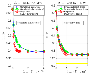
Figure 1: $\mathsf{LOLP}$ vs battery size for $d=$ 1800 MW ($\Delta<0$)

Note that in all the plots, the simlulated $\mathsf{LOLP}$ from our CTMC model closely matches the simulated $\mathsf{LOLP}$ from the DTMC model. This essentially validates our first order Taylor approximation for fitting the transition rate matrix $Q$ from the empirical transition probability matrix $T.$ Moreover, we note that the simulated $\mathsf{LOLP}$ from the Markov models more closely matches the empirical $\mathsf{LOLP}$ for the stationary wind data than for the entire time series. This suggests that the Markov models are a better fit on the stationary data than on the complete, highly non-stationary time series. In practice, this means we should fit different Markov models to capture wind variability in different parts of the day in each season.

Focusing specifically on Figure 1, which corresponds to the negative drift scenario, we make the following observations.

• The empirical as well as simulated $\mathsf{LOLP}$ converges, as $b_{\max}$ becomes large, to a value which is lower bounded by the bound specified in Theorem 1.

• The empirical $\mathsf{LOLP}$ is less than the $\mathsf{LOLP}$ implied by the Markov models. In other words, our models tend to overestimate the $\mathsf{LOLP}.$

• The $\mathsf{LOLP}$ corresponding to a given battery size is greater for the entire time series as compared to the stationary data, suggesting that the former dataset is more ‘variable’ than the latter.

Focusing next on Figure 2, which corresponds to the positive drift scenario, we note that the $\mathsf{LOLP}$ decays to zero as $b_{\max}$ becomes large, consistent with Theorem 2. Moreover, we see that the Markov models tend to overestimate the $\mathsf{LOLP}$ (as before). To illustrate the exponential decay of $\mathsf{LOLP}$ with battery size clearly, we plot the simulated $\mathsf{LOLP}$ from the CTMC model on a log-linear scale in Figure 3. Note that the plot looks asymptotically linear (establishing the exponential decay), with a slope that closely matches the decay rate from Theorem 2.

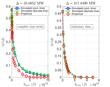
Figure 2: $\mathsf{LOLP}$ vs battery size for $d=$ 1200 MW ($\Delta>0$)

IV-D Battery sizing

The above results support our claim that when $\Delta>0,$ the $\mathsf{LOLP}$ decays exponentially with battery size with a decay rate equal to $\lambda.$ In other words, when $b_{\max}$ is large, the $\mathsf{LOLP}$ may be approximated as

$$\mathsf{LOLP}\approx ce^{-\lambda b_{\max}}.$$ (7)

This further implies that the battery size required to maintain the $\mathsf{LOLP}$ at $\delta$ is given by

$$b_{\max}\approx\frac{\log(c)}{\lambda}+\frac{\log(1/\delta)}{\lambda}.$$

Since the pre-factor $c$ in (7) is unknown here, a natural approximation would be to estimate the battery size required as

$$b_{\max}\approx\frac{\log(1/\delta)}{\lambda}.$$ (8)

Clearly, we would expect the above estimate to be accurate upto an additive offset. Moreover, we would expect that the error of our estimate would be small in relative terms for small $\delta.$

To validate (8), consider the CTMC model for the stationary wind data, with $d=1200$ MW. For this model, we compare the minimum storage size required to bring the simulated $\mathsf{LOLP}$ below $\delta$ with the estimate (8); see the left panel of Figure 4. Notice the constant offset between the two curves, as predicted. However, we note the (unknown) offset results in a roughly 40% error in battery size requirement when $\delta=10^{-3}.$ For lower values of $\delta,$ the relative error would of course be smaller. This means that for moderate values of reliability target $\delta,$ the estimate (8) can be used to make ballpark estimates of the storage size required.

However, (7) can also be used for relative storage sizing as follows: Note that (7) suggests that shrinking the $\mathsf{LOLP}$ be a factor of $\epsilon$ would require an increase in battery size of $\frac{\log(1/\epsilon)}{\lambda}.$ To validate this approximation, we consider the following baseline scenario. Setting $d=1200$ MW with the stationary wind data, and $b_{\max}=0.25\times 10^{12}$ J, the simulated $\mathsf{LOLP}$ equals $L=0.018.$ In the right panel of Figure 4, we plot the additional battery size required to make the $\mathsf{LOLP}$ $L/\epsilon$ versus $\epsilon,$ using the above approximation, as well as by simulating the CTMC model. Note that the approximation is remarkably accurate, even for moderate values of $\mathsf{LOLP}.$

This shows that (7) is an accurate description of the $\mathsf{LOLP}$ as $b_{\max}$ becomes large, and can be used in practice to guide battery sizing decisions.

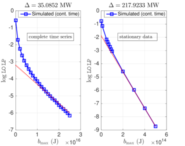
Figure 3: Simulated $\mathsf{LOLP}$ vs battery size plot on $\log$-linear scale for for $d=$ 1200 MW (positive drift). The dotted red line has slope $-\lambda.$

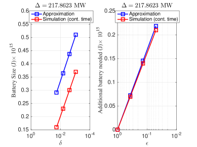
Figure 4: Validation of battery sizing approximations

V Concluding Remarks

In this paper, we developed an analytical framework for characterizing the reliability of a renewable generator bundled with a battery. We analysed how the reliability, captured by the $\mathsf{LOLP},$ scales as the battery size increases. Our results highlight the achievable limits of reliability, and provide useful guidelines for sizing storage in practice.

While we have used $\mathsf{LOLP}$ as the reliability metric throughout this paper, it should be noted that our conclusions extend readily to another related metric, i.e., lost load rate ($\mathsf{LLR}$), which is defined as the long run rate of unserved load, i.e.,

$$\mathsf{LLR}=\sum_{i\in S_{-}}F_{i}(0)(-r_{i}).$$

Since there exists positive constants $c_{1}$ and $c_{2}$ such that

$$c_{1}\mathsf{LOLP}\leq\mathsf{LLR}\leq c_{2}\mathsf{LOLP},$$

our asymptotic characterizations of $\mathsf{LOLP}$ as $b_{\max}\rightarrow\infty$ extend readily to $\mathsf{LLR}.$ Indeed, when $\Delta<0,$ $\mathsf{LLR}>-\Delta.$ When $\Delta>0,$ $\mathsf{LLR}$ decays exponentially with $b_{\max}$ with the same decay rate $\lambda$ as the one characterized in Theorem 2 for $\mathsf{LOLP}.$

This work motivates future research along several directions. We believe our formulations are a natural first step to analyse the economies of scale that would result from sharing of storage, between renewable generators or electricity prosumers; we show a result along these lines in [13]. Another direction is performing a similar reliability calculation with for a network of generators, taking into account transmission constraints. Finally, we note that our work motivates more sound stochastic modeling of renewable generation, to improve the real-world applicability of analytical reliability characterizations (as in the present paper).

Appendix A Proof of Theorem 1

The proof of Theorem 1 is based on energy conservation of the battery content together with the law of large numbers applied to the background Markov process. Let $\mathcal{O}_{cum}(t)$ be the total amount of wasted energy due to battery overflow in the interval $[0,t].$ Similarly, let $\ell_{cum}(t)$ be the total amount of unserved energy demand in the same interval (during loss of load). Let $d_{cum}(t)$ be the net demand served over the interval $[0,t]$ and $g_{cum}(t)$ be total generation over the same interval. Finally, define

$$\ell_{avg}:=\lim_{t\to\infty}\frac{\ell_{cum}(t)}{t}\ \ \ \ \mathcal{O}_{avg}:=\lim_{t\to\infty}\frac{\mathcal{O}_{cum}(t)}{t}.$$

Recall that $\underline{r}:=\min\{r_{i},\ i=1,\ldots,|S|\}.$ Let $\bar{r}:=\max\{r_{i},\ i=1,\ldots,|S|\}$. With these notations we have the following result.

Lemma 3.

$\ell_{avg}=-\Delta+\mathcal{O}_{avg}>-\Delta$. If the drift is negative, i.e., $\Delta<0,$ then $\lim_{b_{\max}\to\infty}\ell_{avg}=-\Delta$.

Proof:

Applying energy conservation, we get

$$g_{cum}(t)-\mathcal{O}_{cum}(t)=d_{cum}(t)-\ell_{cum}(t)+b(t)$$

$$\Rightarrow\frac{\ell_{cum}}{t} =-\frac{(g_{cum}(t)-d_{cum}(t))}{t}+\frac{\mathcal{O}_{cum}(t)}{t}+\frac{b(t)}{t}$$

$$\Rightarrow\frac{\ell_{cum}}{t} =-\frac{1}{t}\int_{0}^{t}r_{X(s)}ds+\frac{\mathcal{O}_{cum}(t)}{t}+\frac{b(t)}{t}$$

$$\Rightarrow\lim_{t\to\infty}\frac{\ell_{cum}}{t} =-\lim_{t\to\infty}\frac{1}{t}\int_{0}^{t}r_{X(s)}ds+\lim_{t\to\infty}\frac{\mathcal{O}_{cum}(t)}{t}$$

$$\quad+\lim_{t\to\infty}\frac{b(t)}{t}.$$

Since the battery capacity is finite, $\lim\limits_{t\to\infty}\frac{b(t)}{t}=0$ and law of large numbers for Markov chains implies that $\lim_{t\to\infty}\frac{1}{t}\int_{0}^{t}r_{X(s)}ds=\Delta$. Therefore we get

$$\ell_{avg}=\lim_{t\to\infty}\frac{\ell_{cum}}{t}=-\Delta+\mathcal{O}_{avg}.$$

It is easy to see that

$$\mathcal{O}_{avg}\leq\bar{r}\ \mathbb{P}[b=b_{\max}]\leq\bar{r}\ \mathbb{P}[b_{\infty}\geq b_{\max}],$$

where $b_{\infty}$ denotes the stationary buffer occupancy in an infinite buffer system seeing the same net generation process. When the drift is negative, as $b_{\max}\rightarrow\infty$, $\mathbb{P}[b_{\infty}\geq b_{\max}]$ decays exponentially with $b_{\max}$ (see [5]), which implies that

$$\lim_{b_{\max}\to\infty}\ell_{avg}=-\Delta.$$

 

With this result we now prove Theorem 1.

Proof:

It is not hard to see that

$$\ell_{avg}=\lim_{t\to\infty}\frac{\ell_{cum}(t)}{t}\leq-\underline{r}\mathsf{LOLP}.$$

From Lemma 3, $\ell_{avg}\geq-\Delta.$ Therefore,

$$\mathsf{LOLP}\geq\frac{-\Delta}{-\underline{r}}.$$

When the background CTMC has only a single state of discharge, i.e., $|S_{-}|=1$, then $\ell_{avg}=-\underline{r}\mathsf{LOLP}$. From Lemma 3, $\lim_{b_{\max}\to\infty}\ell_{avg}=-\Delta$ which gives us

$$\lim_{b_{\max}\to\infty}\mathsf{LOLP}=\frac{-\Delta}{-\underline{r}}.$$

 

Appendix B Decay rate for $\Delta>0$

B-A Proof of Lemma 1

Let the sequence $\{b^{r}_{\infty}[n]\}$ denote the buffer occupancy in the infinite buffer reversed system, sampled at the transition instants of the (uniformized) background process $X(t).$ We have

$$b^{r}_{\infty}[n+1]=(b^{r}_{\infty}[n]-r_{X_{n}}Y_{n})_{+},$$ (9)

where $(z)_{+}=\max(z,0).$ Since the discrete-time process $\{b^{r}_{\infty}[\cdot]\}$ is obtained by sampling the continuous-time process $\{b^{r}_{\infty}(\cdot)\}$ at the instants of a Poisson process (of rate $q$), the PASTA property (see [14]) implies that the time averages corresponding to both coincide. Moreover, (9) is a Lindley recursion (see [15]) with negative drift (since $\Delta^{r}<0$). The logarithmic asymptotics of $\mathbb{P}\left[b^{r}_{\infty}\geq B\right]$ thus follow (see Theorem 3.1 in [15]) once we verify that the function $\Lambda(\cdot)$ is well defined and satisfies the Gartner-Ellis conditions [7]. This is done in Lemma 4 below.

The function $\Lambda(\cdot)$ is characterized as follows.

Lemma 4.

$$\Lambda(\theta)=\left\{\begin{array}[]{ll}\log(\rho_{M(\theta)})&\theta\in\left(\nicefrac{{-q}}{{\bar{r}}},\nicefrac{{-q}}{{\underline{r}}}\right)\\ \infty&\text{ elsewhere}\end{array}\right.,$$

where $\rho_{M(\theta)}$ is the Perron Frobenious eigenvalue corresponding to the matrix $M(\theta),$ defined as

$$M_{l,m}(\theta)=P_{l,m}\frac{q}{q+\theta r_{l}},$$

where recall that $P$ is the transition probability matrix of the embedded Markov chain $\{Z_{k}\}$. Moreover, $\Lambda(\cdot)$ is convex and differentiable over $\left(\nicefrac{{-q}}{{\bar{r}}},\nicefrac{{-q}}{{\underline{r}}}\right),$ $\Lambda^{\prime}(0)<0,$ and

$$\lim_{\theta\uparrow\nicefrac{{-q}}{{\underline{r}}}}\Lambda(\theta)=\lim_{\theta\downarrow\nicefrac{{-q}}{{\bar{r}}}}\Lambda(\theta)=\infty.$$ (10)

Proof.

Throughout the proof, we assume $\theta\in(\nicefrac{{-q}}{{\bar{r}}},\nicefrac{{-q}}{{\underline{r}}}).$ It is not hard to see that $\mathbb{E}\left[e^{\theta U_{k}}\right]=\infty$ if $\theta\notin(\nicefrac{{-q}}{{\bar{r}}},\nicefrac{{-q}}{{\underline{r}}}).$

Define $v_{k}(l)=\mathbb{E}\left[e^{\theta U_{k}}\ |\ X_{0}=l\right],$ $v_{k}=(v_{k}(l),l\in S).$ The vector $v_{k}$ can be expressed inductively as follows.

$$v_{k}(l) =\sum_{m\in S}P_{l,m}\mathbb{E}\left[e^{-\theta\sum_{j=1}^{k}r_{X_{j}}Y_{j}}\ |\ X_{2}=m\right]\mathbb{E}\left[e^{-\theta r_{l}Y_{0}}\right]$$

$$=\sum_{m\in S}P_{l,m}\frac{q}{q+\theta r_{l}}v_{k-1}(m)$$

$$=\sum_{m\in S}M_{l,m}(\theta)v_{k-1}(m)$$

Thus, $v_{k}=M(\theta)v_{k-1}=M^{k}(\theta)v_{0}.$ Denoting the law of the Markov process at time $0$ by the row vector $\pi_{0},$

$$\mathbb{E}\left[e^{\theta U_{k}}\right]=\pi_{0}M^{k}(\theta)v_{0}.$$

That

$$\lim_{k\rightarrow\infty}\frac{\log\mathbb{E}\left[e^{\theta U_{k}}\right]}{k}=\rho_{M(\theta)}$$

now follows from the Perron Frobenius theorem [7, Theorem 3.1.1].

That $\Lambda(\cdot)$ is convex follows from the fact that it is pointwise limit of convex functions. Its differentiability follows from the differentiability of Perron Frobenius eigenvalue of a non-negative matrix with respect to its entries. That $\Lambda^{\prime}(0)<0$ follows from Lemma 3.2 in [15].

Finally, to show (10), we use $\rho(M(\theta))\geq\rho(G(\theta)),$ where $G(\theta)$ is a symmetric non-negative matrix defined as

$$G_{s,s^{\prime}}(\theta)=\sqrt{M_{s,s^{\prime}}(\theta)M_{s^{\prime},s}(\theta)};$$

(see Theorem 2 in [16]). It therefore suffices to show that $\rho(G(\theta))\rightarrow\infty$ as $\theta\uparrow\nicefrac{{-q}}{{\underline{r}}}$ and $\theta\downarrow\nicefrac{{-q}}{{\bar{r}}},$ which follows trivially from the observation that $\mathrm{trace}(G(\theta))\rightarrow\infty$ along each of the above limits (note that all diagonal entries of $G$ are positive).  

B-B Proof of Lemma 2

Lemma B-B follows from standard techniques in large deviations theory that show that the decay rates associated with $\mathbb{P}\left[b^{r}=b_{\max}\right]$ and $\mathbb{P}\left[b^{r}_{\infty}\geq b_{\max}\right]$ as $b_{\max}\rightarrow\infty$ are the same under very general conditions; see [17] and [15, Section 6.5].

References

- [1] V. Deulkar, J. Nair, and A. A. Kulkarni, “Sizing Storage for Reliable Renewable Integration,” in IEEE PowerTech, 2019.
- [2] E. S. Association, “U.S. Energy Storage Project Pipeline Doubles in 2018, Nears 33 GW,” http://www.energystorage.org/news/esa-news/us-energy-storage-project-pipeline-doubles-2018-nears-33-gw/, 2018, [Online; accessed 7-December-2018].
- [3] E. I. Administration, “U.S. Battery Storage Market Trends,” https://www.eia.gov/analysis/studies/electricity/batterystorage/, 2018, [Online; accessed 7-December-2018].
- [4] D. Anick, D. Mitra, and M. M. Sondhi, “Stochastic theory of a data-handling system with multiple sources,” Bell System Technical Journal, vol. 61, no. 8, pp. 1871–1894, 1982.
- [5] D. Mitra, “Stochastic theory of a fluid model of producers and consumers coupled by a buffer,” Advances in Applied Probability, vol. 20, no. 3, pp. 646–676, 1988.
- [6] M. Kijima, Markov processes for stochastic modeling. CRC Press, 1997, vol. 6.
- [7] A. Dembo and O. Zeitouni, Large deviations techniques and applications. Springer, 1998.
- [8] B. P. Administration, “Wind flow data,” https://transmission.bpa.gov/business/operations/wind/, 2018, [Online; accessed 20-November-2018].
- [9] K. Brokish and J. Kirtley, “Pitfalls of modeling wind power using markov chains,” in Power Systems Conference and Exposition, 2009. PSCE’09. IEEE/PES. IEEE, 2009, pp. 1–6.
- [10] H. Nfaoui, H. Essiarab, and A. Sayigh, “A stochastic markov chain model for simulating wind speed time series at tangiers, morocco,” Renewable Energy, vol. 29, no. 8, pp. 1407–1418, 2004.
- [11] A. Shamshad, M. Bawadi, W. W. Hussin, T. Majid, and S. Sanusi, “First and second order markov chain models for synthetic generation of wind speed time series,” Energy, vol. 30, no. 5, pp. 693–708, 2005.
- [12] G. Papaefthymiou and B. Klockl, “Mcmc for wind power simulation,” IEEE transactions on energy conversion, vol. 23, no. 1, pp. 234–240, 2008.
- [13] J. Nair, A. A. Kulkarni, and V. Deulkar, “Statistical economies of scale in battery sharing via large deviations,” in IEEE Conference on Decision and Control, under review, 2019.
- [14] R. W. Wolff, “Poisson arrivals see time averages,” Operations Research, vol. 30, no. 2, pp. 223–231, 1982.
- [15] A. J. Ganesh, N. O’Connell, and D. J. Wischik, Big queues. Springer, 2004.
- [16] A. J. Schwenk, “Tight bounds on the spectral radius of asymmetric nonnegative matrices,” Linear algebra and its applications, vol. 75, pp. 257–265, 1986.
- [17] F. Toomey, “Bursty traffic and finite capacity queues,” Annals of Operations Research, vol. 79, pp. 45–62, 1998.