Hypothesis Set Stability and Generalization

Abstract

We present a study of generalization for data-dependent hypothesis sets. We give a general learning guarantee for data-dependent hypothesis sets based on a notion of transductive Rademacher complexity. Our main result is a generalization bound for data-dependent hypothesis sets expressed in terms of a notion of hypothesis set stability and a notion of Rademacher complexity for data-dependent hypothesis sets that we introduce. This bound admits as special cases both standard Rademacher complexity bounds and algorithm-dependent uniform stability bounds. We also illustrate the use of these learning bounds in the analysis of several scenarios.

1 Introduction

Most generalization bounds in learning theory hold for a fixed hypothesis set, selected before receiving a sample. This includes learning bounds based on covering numbers, VC-dimension, pseudo-dimension, Rademacher complexity, local Rademacher complexity, and other complexity measures (Pollard, 1984; Zhang, 2002; Vapnik, 1998; Koltchinskii and Panchenko, 2002; Bartlett et al., 2002). Some alternative guarantees have also been derived for specific algorithms. Among them, the most general family is that of uniform stability bounds given by Bousquet and Elisseeff (2002). These bounds were recently significantly improved by Feldman and Vondrak (2019), who proved guarantees that are informative, even when the stability parameter $\beta$ is only in $o(1)$, as opposed to $o(1/\sqrt{m})$. The $\log^{2}m$ factor in these bounds was later reduced to $\log m$ by Bousquet et al. (2019). Bounds for a restricted class of algorithms were also recently presented by Maurer (2017), under a number of assumptions on the smoothness of the loss function. Appendix A gives more background on stability.

In practice, machine learning engineers commonly resort to hypothesis sets depending on the same sample as the one used for training. This includes instances where a regularization, a feature transformation, or a data normalization is selected using the training sample, or other instances where the family of predictors is restricted to a smaller class based on the sample received. In other instances, as is common in deep learning, the data representation and the predictor are learned using the same sample. In ensemble learning, the sample used to train models sometimes coincides with the one used to determine their aggregation weights. However, standard generalization bounds are not directly applicable for these scenarios since they assume a fixed hypothesis set.

1.1 Contributions of this paper.

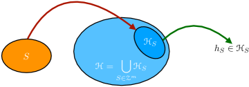
Figure 1: Decomposition of the learning algorithm’s hypothesis selection into two stages. In the first stage, the algorithm determines a hypothesis ${\mathscr{H}}_{S}$ associated to the training sample $S$ which may be a small subset of the set of all hypotheses that could be considered, say ${\mathscr{H}}=\bigcup_{S\in{\mathscr{Z}}^{m}}{\mathscr{H}}_{S}$. The second stage then consists of selecting a hypothesis $h_{S}$ out of ${\mathscr{H}}_{S}$.

1. Foundational definitions of data-dependent hypothesis sets. We present foundational definitions of learning algorithms that rely on data-dependent hypothesis sets. Here, the algorithm decomposes into two stages: a first stage where the algorithm, on receiving the sample $S$, chooses a hypothesis set ${\mathscr{H}}_{S}$ dependent on $S$, and a second stage where a hypothesis $h_{S}$ is selected from ${\mathscr{H}}_{S}$. Standard generalization bounds correspond to the case where ${\mathscr{H}}_{S}$ is equal to some fixed ${\mathscr{H}}$ independent of $S$. Algorithm-dependent analyses, such as uniform stability bounds, coincide with the case where ${\mathscr{H}}_{S}$ is chosen to be a singleton ${\mathscr{H}}_{S}=\{h_{S}\}$. Thus, the scenario we study covers both existing settings and other intermediate scenarios. Figure 1 illustrates our general scenario.

2. Learning bounds via transductive Rademacher complexity. We present general learning bounds for data-dependent hypothesis sets using a notion of transductive Rademacher complexity (Section 3). These bounds hold for arbitrary bounded losses and improve upon previous guarantees given by Gat (2001) and Cannon et al. (2002) for the binary loss, which were expressed in terms of a notion of shattering coefficient adapted to the data-dependent case, and are more explicit than the guarantees presented by Philips (2005)[corollary 4.6 or theorem 4.7]. Nevertheless, such bounds may often not be sufficiently informative, since they ignore the relationship between hypothesis sets based on similar samples.

3. Learning bounds via hypothesis set stability. We provide finer generalization bounds based on the key notion of hypothesis set stability that we introduce in this paper. This notion admits algorithmic stability as a special case, when the hypotheses sets are reduced to singletons. We also introduce a new notion of Rademacher complexity for data-dependent hypothesis sets. Our main results are generalization bounds (Section 4) for stable data-dependent hypothesis sets expressed in terms of the hypothesis set stability parameter, our notion of Rademacher complexity, and a notion of cross-validation stability that, in turn, can be upper-bounded by the diameter of the family of hypothesis sets. Our learning bounds admit as special cases both standard Rademacher complexity bounds and algorithm-dependent uniform stability bounds.

4. New generalization bounds for specific learning applications. In section 5 (see also Appendix G), we illustrate the generality and the benefits of our hypothesis set stability learning bounds by using them to derive new generalization bounds for several learning applications. To our knowledge, there is no straightforward analysis based on previously existing tools that yield these generalization bounds. These applications include: (a) bagging algorithms that may employ non-uniform, data-dependent, averaging of the base predictors, (b) stochastic strongly-convex optimization algorithms based on an average of other stochastic optimization algorithms, (c) stable representation learning algorithms, which first learn a data representation using the sample and then learn a predictor on top of the learned representation, and (d) distillation algorithms, which first compute a complex predictor using the sample and then use it to learn a simpler predictor that is close to it.

1.2 Related work on data-dependent hypothesis sets.

Shawe-Taylor et al. (1998) presented an analysis of structural risk minimization over data-dependent hierarchies based on a concept of luckiness, which generalizes the notion of margin of linear classifiers. Their analysis can be viewed as an alternative and general study of data-dependent hypothesis sets, using luckiness functions and $\omega$-smallness (or $\omega$-smoothness) conditions. A luckiness function helps decompose a hypothesis set into lucky sets, that is sets of functions luckier than a given function. The luckiness framework is attractive and the notion of luckiness, for example margin, can in fact be combined with our results. However, finding pairs of truly data-dependent luckiness and $\omega$-smallness functions, other than those based on the margin and the empirical VC-dimension, is quite difficult, in particular because of the very technical $\omega$-smallness condition (see Philips, 2005, p. 70). In contrast, hypothesis set stability is simpler and often easier to bound. The notions of luckiness and $\omega$-smallness have also been used by Herbrich and Williamson (2002) to derive algorithm-specific guarantees. In fact, the authors show a connection with algorithmic stability (not hypothesis set stability), at the price of a guarantee requiring the strong condition that the stability parameter be in $o(1/m)$, where $m$ is the sample size (see Herbrich and Williamson, 2002, pp. 189-190).

Data-dependent hypothesis classes are conceptually related to the notion of data-dependent priors in PAC-Bayesian generalization bounds. Catoni (2007) developed localized PAC-Bayes analysis by using a prior defined in terms of the data generating distribution. This work was extended by Lever et al. (2013) who proved sharp risk bounds for stochastic exponential weights algorithms. Parrado-Hernández et al. (2012) investigated the possibility of learning the prior from a separate data set, as well as priors obtained via computing a data-dependent bound on the KL term. More closely related to this paper is the work of Dziugaite and Roy (2018a, b), who develop PAC-Bayes bounds by choosing the prior via a data-dependent differentially private mechanism, and also showed that weaker notions than differential privacy also suffice to yield valid bounds. In Appendix H, we give a more detailed discussion of PAC-Bayes bounds, in particular to show how finer PAC-Bayes bounds than standard ones can be derived from Rademacher complexity bounds, here with an alternative analysis and constants than (Kakade et al., 2008) and how data-dependent PAC-Bayes bounds can be derived from our data-dependent Rademacher complexity bounds. More discussion on data-dependent priors can be found in Appendix F.3.

2 Definitions and Properties

Let ${\mathscr{X}}$ be the input space and ${\mathscr{Y}}$ the output space, and define ${\mathscr{Z}}:={\mathscr{X}}\times{\mathscr{Y}}$ We denote by ${\mathscr{D}}$ the unknown distribution over ${\mathscr{X}}\times{\mathscr{Y}}$ according to which samples are drawn.

The hypotheses $h$ we consider map ${\mathscr{X}}$ to a set ${\mathscr{Y}}^{\prime}$ sometimes different from ${\mathscr{Y}}$. For example, in binary classification, we may have ${\mathscr{Y}}=\{-1,+1\}$ and ${\mathscr{Y}}^{\prime}=\mathbb{R}$. Thus, we denote by $\ell\colon{\mathscr{Y}}^{\prime}\times{\mathscr{Y}}\to[0,1]$ a loss function defined on ${\mathscr{Y}}^{\prime}\times{\mathscr{Y}}$ and taking non-negative real values bounded by one. We denote the loss of a hypothesis $h\colon{\mathscr{X}}\to{\mathscr{Y}}^{\prime}$ at point $z=(x,y)\in{\mathscr{X}}\times{\mathscr{Y}}$ by $L(h,z)=\ell(h(x),y)$. We denote by $R(h)$ the generalization error or expected loss of a hypothesis $h\in{\mathscr{H}}$ and by $\widehat{R}_{S}(h)$ its empirical loss over a sample $S=(z_{1},\ldots,z_{m})$:

$$R(h)=\operatorname*{\mathbb{E}}_{z\sim{\mathscr{D}}}[L(h,z)]\qquad\widehat{R}_{S}(h)=\operatorname*{\mathbb{E}}_{z\sim S}[L(h,z)]=\frac{1}{m}\sum_{i=1}^{m}L(h,z_{i}).$$

In the general framework we consider, a hypothesis set depends on the sample received. We will denote by ${\mathscr{H}}_{S}$ the hypothesis set depending on the labeled sample $S\in{\mathscr{Z}}^{m}$ of size $m\geq 1$. We assume that ${\mathscr{H}}_{S}$ is invariant to the ordering of the points in $S$.

Definition 1 (Hypothesis set uniform stability).

Fix $m\geq 1$. We will say that a family of data-dependent hypothesis sets $\mathcal{H}=({\mathscr{H}}_{S})_{S\in{\mathscr{Z}}^{m}}$ is $\beta$-uniformly stable (or simply $\beta$-stable) for some $\beta\geq 0$, if for any two samples $S$ and $S^{\prime}$ of size $m$ differing only by one point, the following holds:

$$\forall h\in{\mathscr{H}}_{S},\exists h^{\prime}\in{\mathscr{H}}_{S^{\prime}}\colon\,\forall z\in{\mathscr{Z}},|L(h,z)-L(h^{\prime},z)|\leq\beta.$$ (1)

Thus, two hypothesis sets derived from samples differing by one element are close in the sense that any hypothesis in one admits a counterpart in the other set with $\beta$-similar losses. A closely related notion is the sensitivity of a function $f\colon{\mathscr{Z}}^{m}\to\mathbb{R}$. Such a function $f$ is called $\beta$-sensitive if for any two samples $S$ and $S^{\prime}$ of size $m$ differing only by one point, we have $|f(S)-f(S^{\prime})|\leq\beta$.

We also introduce a new notion of Rademacher complexity for data-dependent hypothesis sets. To introduce its definition, for any two samples $S,T\in{\mathscr{Z}}^{m}$ and a vector of Rademacher variables ${\boldsymbol{\sigma}}$, denote by $S_{T,{\boldsymbol{\sigma}}}$ the sample derived from $S$ by replacing its $i$th element with the $i$th element of $T$, for all $i\in[m]=\{1,2,\ldots,m\}$ with $\sigma_{i}=-1$. We will use ${\mathscr{H}}_{S,T}^{\boldsymbol{\sigma}}$ to denote the hypothesis set ${\mathscr{H}}_{S_{T,{\boldsymbol{\sigma}}}}$.

Definition 2 (Rademacher complexity of data-dependent hypothesis sets).

Fix $m\geq 1$. The empirical Rademacher complexity $\widehat{\mathfrak{R}}^{\diamond}_{S,T}(\mathcal{H})$ and the Rademacher complexity $\mathfrak{R}^{\diamond}_{m}(\mathcal{H})$ of a family of data-dependent hypothesis sets $\mathcal{H}=({\mathscr{H}}_{S})_{S\in{\mathscr{Z}}^{m}}$ for two samples $S=(z^{S}_{1},\ldots,z^{S}_{m})$ and $T=(z^{T}_{1},\ldots,z^{T}_{m})$ in ${\mathscr{Z}}^{m}$ are defined by

$$\widehat{\mathfrak{R}}^{\diamond}_{S,T}(\mathcal{H})=\frac{1}{m}\operatorname*{\mathbb{E}}_{{\boldsymbol{\sigma}}}\Bigg{[}\sup_{h\in{\mathscr{H}}_{S,T}^{\boldsymbol{\sigma}}}\sum_{i=1}^{m}\sigma_{i}h(z^{T}_{i})\Bigg{]}\qquad\mathfrak{R}^{\diamond}_{m}(\mathcal{H})=\frac{1}{m}\operatorname*{\mathbb{E}}_{\begin{subarray}{c}S,T\sim{\mathscr{D}}^{m}\\ {\boldsymbol{\sigma}}\end{subarray}}\Bigg{[}\sup_{h\in{\mathscr{H}}_{S,T}^{\boldsymbol{\sigma}}}\sum_{i=1}^{m}\sigma_{i}h(z^{T}_{i})\Bigg{]}.$$ (2)

When the family of data-dependent hypothesis sets $\mathcal{H}$ is $\beta$-stable with $\beta=O(1/m)$, the empirical Rademacher complexity $\widehat{\mathfrak{R}}^{\diamond}_{S,T}(\mathcal{G})$ is sharply concentrated around its expectation $\mathfrak{R}^{\diamond}_{m}(\mathcal{G})$, as with the standard empirical Rademacher complexity (see Lemma 4).

Let ${\mathscr{H}}_{S,T}$ denote the union of all hypothesis sets based on ${\mathscr{U}}=\{U\colon U\subseteq(S\cup T),U\in{\mathscr{Z}}^{m}\}$, the subsamples of $S\cup T$ of size $m$: ${\mathscr{H}}_{S,T}=\bigcup_{U\in{\mathscr{U}}}{\mathscr{H}}_{U}$. Since for any ${\boldsymbol{\sigma}}$, we have ${\mathscr{H}}_{S,T}^{\boldsymbol{\sigma}}\subseteq{\mathscr{H}}_{S,T}$, the following simpler upper bound in terms of the standard empirical Rademacher complexity of ${\mathscr{H}}_{S,T}$ can be used for our notion of empirical Rademacher complexity:

$$\mathfrak{R}^{\diamond}_{m}(\mathcal{H}) \leq\frac{1}{m}\operatorname*{\mathbb{E}}_{\begin{subarray}{c}S,T\sim{\mathscr{D}}^{m}\\ {\boldsymbol{\sigma}}\end{subarray}}\bigg{[}\sup_{h\in{\mathscr{H}}_{S,T}}\sum_{i=1}^{m}\sigma_{i}h(z^{T}_{i})\bigg{]}=\operatorname*{\mathbb{E}}_{\begin{subarray}{c}S,T\sim{\mathscr{D}}^{m}\end{subarray}}\Big{[}\widehat{\mathfrak{R}}_{T}({\mathscr{H}}_{S,T})\Big{]},$$

where $\widehat{\mathfrak{R}}_{T}({\mathscr{H}}_{S,T})$ is the standard empirical Rademacher complexity of ${\mathscr{H}}_{S,T}$ for the sample $T$. Some properties of our notion of Rademacher complexity are given in Appendix B.

Let ${\mathscr{G}}_{S}$ denote the family of loss functions associated to ${\mathscr{H}}_{S}$:

$${\mathscr{G}}_{S}=\{z\mapsto L(h,z)\colon h\in{\mathscr{H}}_{S}\},$$ (3)

and let $\mathcal{G}=({\mathscr{G}}_{S})_{S\in{\mathscr{Z}}^{m}}$ denote the family of hypothesis sets ${\mathscr{G}}_{S}$. Our main results will be expressed in terms of $\mathfrak{R}^{\diamond}_{m}(\mathcal{G})$. When the loss function $\ell$ is $\mu$-Lipschitz, by Talagrand’s contraction lemma (Ledoux and Talagrand, 1991), in all our results, $\mathfrak{R}^{\diamond}_{m}(\mathcal{G})$ can be replaced by $\mu\operatorname*{\mathbb{E}}_{\begin{subarray}{c}S,T\sim{\mathscr{D}}^{m}\end{subarray}}[\widehat{\mathfrak{R}}_{T}({\mathscr{H}}_{S,T})]$.

Rademacher complexity is one way to measure the capacity of the family of data-dependent hypothesis sets. We also derive learning bounds in situations where a notion of diameter of the hypothesis sets is small. We now define a notion of cross-validation stability and diameter for data-dependent hypothesis sets. In the following, for a sample $S$, $S^{z\leftrightarrow z^{\prime}}$ denotes the sample obtained from $S$ by replacing $z\in S$ by $z^{\prime}\in{\mathscr{Z}}$.

Definition 3 (Hypothesis set Cross-Validation (CV) stability, diameter).

Fix $m\geq 1$. For some $\bar{\chi},\chi,\bar{\Delta},\Delta,\Delta_{\max}\geq 0$, we say that a family of data-dependent hypothesis sets $\mathcal{H}=({\mathscr{H}}_{S})_{S\in{\mathscr{Z}}^{m}}$ has average CV-stability $\bar{\chi}$, CV-stability $\chi$, average diameter $\bar{\Delta}$, diameter $\Delta$ and max-diameter $\Delta_{\max}$ if the following hold:

$$\operatorname*{\mathbb{E}}_{S\sim{\mathscr{D}}^{m}}\operatorname*{\mathbb{E}}_{z^{\prime}\sim{\mathscr{D}},z\sim S}\bigg{[}\sup_{h\in{\mathscr{H}}_{S},h^{\prime}\in{\mathscr{H}}_{S^{z\leftrightarrow z^{\prime}}}}L(h^{\prime},z)-L(h,z)\bigg{]} \leq\bar{\chi}$$ (4)

$$\sup_{S\in{\mathscr{Z}}^{m}}\operatorname*{\mathbb{E}}_{z^{\prime}\sim{\mathscr{D}},z\sim S}\bigg{[}\sup_{h\in{\mathscr{H}}_{S},h^{\prime}\in{\mathscr{H}}_{S^{z\leftrightarrow z^{\prime}}}}L(h^{\prime},z)-L(h,z)\bigg{]} \leq\chi$$ (5)

$$\operatorname*{\mathbb{E}}_{S\sim{\mathscr{D}}^{m}}\operatorname*{\mathbb{E}}_{z\sim S}\bigg{[}\sup_{h,h^{\prime}\in{\mathscr{H}}_{S}}L(h^{\prime},z)-L(h,z)\bigg{]} \leq\bar{\Delta}$$ (6)

$$\sup_{S\in{\mathscr{Z}}^{m}}\operatorname*{\mathbb{E}}_{z\sim S}\bigg{[}\sup_{h,h^{\prime}\in{\mathscr{H}}_{S}}L(h^{\prime},z)-L(h,z)\bigg{]} \leq\Delta$$ (7)

$$\sup_{S\in{\mathscr{Z}}^{m}}\max_{z\in S}\bigg{[}\sup_{h,h^{\prime}\in{\mathscr{H}}_{S}}L(h^{\prime},z)-L(h,z)\bigg{]} \leq\Delta_{\max}.$$ (8)

CV-stability of hypothesis sets can be bounded in terms of their stability and diameter (see straightforward proof in Appendix C).

Lemma 1.

Suppose a family of data-dependent hypothesis sets $\mathcal{H}$ is $\beta$-uniformly stable. Then if it has diameter $\Delta$, then it is $(\Delta+\beta)$-CV-stable, and if it has average diameter $\bar{\Delta}$ then it is $(\bar{\Delta}+\beta)$-average CV-stable.

3 General learning bound for data-dependent hypothesis sets

In this section, we present general learning bounds for data-dependent hypothesis sets that do not make use of the notion of hypothesis set stability. One straightforward idea to derive such guarantees for data-dependent hypothesis sets is to replace the hypothesis set ${\mathscr{H}}_{S}$ depending on the observed sample $S$ by the union of all such hypothesis sets over all samples of size $m$, $\overline{\mathscr{H}}_{m}=\bigcup_{S\in{\mathscr{Z}}^{m}}{\mathscr{H}}_{S}$. However, in general, $\overline{\mathscr{H}}_{m}$ can be very rich, which can lead to uninformative learning bounds. A somewhat better alternative consists of considering the union of all such hypothesis sets for samples of size $m$ included in some supersample $U$ of size $m+n$, with $n\geq 1$, $\overline{\mathscr{H}}_{U,m}=\bigcup_{\begin{subarray}{c}S\in{\mathscr{Z}}^{m}\\ S\subseteq U\mspace{14.0mu}\end{subarray}}{\mathscr{H}}_{S}$. We will derive learning guarantees based on the maximum transductive Rademacher complexity of $\overline{\mathscr{H}}_{U,m}$. There is a trade-off in the choice of $n$: smaller values lead to less complex sets $\overline{\mathscr{H}}_{U,m}$, but they also lead to weaker dependencies on sample sizes. Our bounds are more refined guarantees than the shattering-coefficient bounds originally given for this problem by Gat (2001) in the case $n=m$, and later by Cannon et al. (2002) for any $n\geq 1$. They also apply to arbitrary bounded loss functions and not just the binary loss. They are expressed in terms of the following notion of transductive Rademacher complexity for data-dependent hypothesis sets:

$$\widehat{\mathfrak{R}}^{\diamond}_{U,m}(\mathcal{G})=\operatorname*{\mathbb{E}}_{\boldsymbol{\sigma}}\Bigg{[}\sup_{h\in\overline{\mathscr{H}}_{U,m}}\frac{1}{m+n}\sum_{i=1}^{m+n}\sigma_{i}L(h,z^{U}_{i})\Bigg{]},$$

where $U=(z^{U}_{1},\ldots,z^{U}_{m+n})\in{\mathscr{Z}}^{m+n}$ and where ${\boldsymbol{\sigma}}$ is a vector of $(m+n)$ independent random variables taking value $\frac{m+n}{n}$ with probability $\frac{n}{m+n}$, and $-\frac{m+n}{m}$ with probability $\frac{m}{m+n}$. Our notion of transductive Rademacher complexity is simpler than that of El-Yaniv and Pechyony (2007) (in the data-independent case) and leads to simpler proofs and guarantees. A by-product of our analysis is learning guarantees for standard transductive learning in terms of this notion of transductive Rademacher complexity, which can be of independent interest.

Theorem 1.

Let $\mathcal{H}=({\mathscr{H}}_{S})_{S\in{\mathscr{Z}}^{m}}$ be a family of data-dependent hypothesis sets. Let $\mathcal{G}$ be defined as in (3). Then, for any $\delta>0$, with probability at least $1-\delta$ over the choice of the draw of the sample $S\sim{\mathscr{Z}}^{m}$, the following inequality holds for all $h\in{\mathscr{H}}_{S}$:

$$R(h)\leq\widehat{R}_{S}(h)+\max_{U\in{\mathscr{Z}}^{m+n}}2\widehat{\mathfrak{R}}^{\diamond}_{U,m}(\mathcal{G})+3\sqrt{\left(\tfrac{1}{m}+\tfrac{1}{n}\right)\log(\tfrac{2}{\delta})}+2\sqrt{\left(\tfrac{1}{m}+\tfrac{1}{n}\right)^{3}mn}.$$

Proof.

(Sketch; full proof in Appendix D.) We use the following symmetrization result, which holds for any $\epsilon>0$ with $m\epsilon^{2}\geq 2$ for data-dependent hypothesis sets (Lemma 5, Appendix D):

$$\operatorname*{\mathbb{P}}_{S\sim{\mathscr{D}}^{m}}\bigg{[}\sup_{h\in{\mathscr{H}}_{S}}R(h)-\widehat{R}_{S}(h)>\epsilon\bigg{]}\leq 2\operatorname*{\mathbb{P}}_{\begin{subarray}{c}S\sim{\mathscr{D}}^{m}\\ T\sim{\mathscr{D}}^{n}\mspace{6.0mu}\end{subarray}}\bigg{[}\sup_{h\in{\mathscr{H}}_{S}}\widehat{R}_{T}(h)-\widehat{R}_{S}(h)>\frac{\epsilon}{2}\bigg{]}.$$

To bound the right-hand side, we use an extension of McDiarmid’s inequality to sampling without replacement (Cortes et al., 2008) applied to $\Phi(S)=\sup_{h\in\overline{\mathscr{H}}_{U,m}}\widehat{R}_{T}(h)-\widehat{R}_{S}(h)$. Lemma 6 (Appendix D) is then used to bound $\operatorname*{\mathbb{E}}[\Phi(S)]$ in terms of our notion of transductive Rademacher complexity. ∎

4 Learning bound for stable data-dependent hypothesis sets

In this section, we present our main generalization bounds for data-dependent hypothesis sets.

Theorem 2.

Let $\mathcal{H}=({\mathscr{H}}_{S})_{S\in{\mathscr{Z}}^{m}}$ be a $\beta$-stable family of data-dependent hypothesis sets, with $\bar{\chi}$ average CV-stability, $\chi$ CV-stability and $\Delta_{\max}$ max-diameter. Let $\mathcal{G}$ be defined as in (3). Then, for any $\delta>0$, with probability at least $1-\delta$ over the draw of a sample $S\sim{\mathscr{Z}}^{m}$, the following inequality holds for all $h\in{\mathscr{H}}_{S}$:

$$\forall h\in{\mathscr{H}}_{S},R(h)\leq\widehat{R}_{S}(h)+\min\Bigg{\{} \min\left\{2\mathfrak{R}^{\diamond}_{m}(\mathcal{G}),\bar{\chi}\right\}+(1+2\beta m)\sqrt{\tfrac{1}{2m}\log(\tfrac{1}{\delta})},$$ (9)

$$\sqrt{e}\chi+4\sqrt{(\tfrac{1}{m}+2\beta)\log(\tfrac{6}{\delta})},$$ (10)

$$48(3\beta+\Delta_{\max})\log(m)\log(\tfrac{5m^{3}}{\delta})+\sqrt{\tfrac{4}{m}\log(\tfrac{4}{\delta})}\Bigg{\}}.$$ (11)

The proof of the theorem is given in Appendix E. The main idea is to control the sensitivity of the function $\Psi(S,S^{\prime})$ defined for any two samples $S,S^{\prime}$, as follows:

$$\Psi(S,S^{\prime})=\sup_{h\in{\mathscr{H}}_{S}}R(h)-\widehat{R}_{S^{\prime}}(h).$$

To prove bound (9), we apply McDiarmid’s inequality to $\Psi(S,S)$, using the $(\frac{1}{m}+2\beta)$-sensitivity of $\Psi(S,S)$, and then upper bound the expectation $\operatorname*{\mathbb{E}}_{S\sim{\mathscr{D}}^{m}}[\Psi(S,S)]$ in terms of our notion of Rademacher complexity. The bound (10) is obtained via a differential-privacy-based technique, as in Feldman and Vondrak (2018), and (11) is a direct consequence of the bound of Feldman and Vondrak (2019) using the observation that an algorithm that chooses an arbitrary $h\in{\mathscr{H}}_{S}$ is $O(\beta+\Delta_{\max})$-uniformly stable in the classical (Bousquet and Elisseeff, 2002) sense.

Bound (9) admits as a special case the standard Rademacher complexity bound for fixed hypothesis sets (Koltchinskii and Panchenko, 2002; Bartlett and Mendelson, 2002): in that case, we have $\mathcal{H}_{S}={\mathscr{H}}$ for some ${\mathscr{H}}$, thus $\mathfrak{R}^{\diamond}_{m}(\mathcal{G})$ coincides with the standard Rademacher complexity $\mathfrak{R}_{m}(\mathcal{G})$; furthermore, the family of hypothesis sets is $0$-stable, thus the bound holds with $\beta=0$.

Bounds (10) and (11) specialize to the bounds of Feldman and Vondrak (2018) and Feldman and Vondrak (2019) respectively for the special case of standard uniform stability of algorithms, since in that case, ${\mathscr{H}}_{S}$ is reduced to a singleton, ${\mathscr{H}}_{S}=\{h_{S}\}$, and so $\Delta=0$, which implies that $\chi\leq\Delta+\beta=\beta$.

The Rademacher complexity-based bound (9) typically gives the tightest control on generalization error compared to the bounds (10) and (11), which rely on the cruder diameter notion. However the diameter may be easier to bound for some applications than the Rademacher complexity. To compare the diameter-based bounds, in applications where $\Delta_{\max}=O(\Delta)$, bound (11) may be tighter than (10). But, in several applications, we have $\beta=O(\frac{1}{m})$, and then bound (10) is tighter.

5 Applications

We now discuss several applications of our learning guarantees, with some others in Appendix G.

5.1 Bagging

Bagging (Breiman, 1996) is a prominent ensemble method used to improve the stability of learning algorithms. It consists of generating $k$ new samples $B_{1},B_{2},\ldots,B_{k}$, each of size $p$, by sampling uniformly with replacement from the original sample $S$ of size $m$. An algorithm $\mathcal{A}$ is then trained on each of these samples to generate $k$ predictors $\mathcal{A}(B_{i})$, $i\in[k]$. In regression, the predictors are combined by taking a convex combination $\sum_{i=1}^{k}w_{i}\mathcal{A}(B_{i})$. Here, we analyze a common instance of bagging to illustrate the application of our learning guarantees: we will assume a regression setting and a uniform sampling from $S$ without replacement. We will also assume that the loss function is $\mu$-Lipschitz in its first argument, that the predictions are in the range $[0,1]$, and that all the mixing weights $w_{i}$ are bounded by $\frac{C}{k}$ for some constant $C\geq 1$, in order to ensure that no subsample $B_{i}$ is overly influential in the final regressor (in practice, a uniform mixture is typically used in bagging).

To analyze bagging, we cast it in our framework. First, to deal with the randomness in choosing the subsamples, we can equivalently imagine the process as choosing indices in $[m]$ to form the subsamples rather than samples in $S$, and then once $S$ is drawn, the subsamples are generated by filling in the samples at the corresponding indexes. For any index $i\in[m]$, the chance that it is picked in any subsample is $\frac{p}{m}$. Thus, by Chernoff’s bound, with probability at least $1-\delta$, no index in $[m]$ appears in more than $t:=\frac{kp}{m}+\sqrt{\frac{2kp\log(\frac{m}{\delta})}{m}}$ subsamples. In the following, we condition on the random seed of the bagging algorithm so that this is indeed the case, and later use a union bound to control the chance that the chosen random seed does not satisfy this property, as elucidated in section F.2.

Define the data-dependent family of hypothesis sets $\mathcal{H}$ as ${\mathscr{H}}_{S}:=\big{\{}\sum_{i=1}^{k}w_{i}\mathcal{A}(B_{i})\colon\,w\in\Delta_{k}^{C/k}\big{\}}$, where $\Delta^{C/k}_{k}$ denotes the simplex of distributions over $k$ items with all weights $w_{i}\leq\frac{C}{k}$. Next, we give upper bounds on the hypothesis set stability and the Rademacher complexity of $\mathcal{H}$. Assume that algorithm $\mathcal{A}$ admits uniform stability $\beta_{A}$ (Bousquet and Elisseeff, 2002), i.e. for any two samples $B$ and $B^{\prime}$ of size $p$ that differ in exactly one data point and for all $x\in\mathcal{X}$, we have $|\mathcal{A}(B)(x)-\mathcal{A}(B^{\prime})(x)|\leq\beta_{\mathcal{A}}$. Now, let $S$ and $S^{\prime}$ be two samples of size $m$ differing by one point at the same index, $z\in S$ and $z^{\prime}\in S^{\prime}$. Then, consider the subsets $B^{\prime}_{i}$ of $S^{\prime}$ which are obtained from the $B_{i}$s by copying over all the elements except $z$, and replacing all instances of $z$ by $z^{\prime}$. For any $B_{i}$, if $z\notin B_{i}$, then $\mathcal{A}(B_{i})=\mathcal{A}(B^{\prime}_{i})$ and, if $z\in B_{i}$, then $|\mathcal{A}(B_{i})(x)-\mathcal{A}(B^{\prime}_{i})(x)|\leq\beta_{\mathcal{A}}$ for any $x\in\mathcal{X}$. We can now bound the hypothesis set uniform stability as follows: since $L$ is $\mu$-Lipschitz in the prediction, for any $z^{\prime\prime}\in\mathcal{Z}$, and any $w\in\Delta^{C/k}_{k}$, we have

$$\Big{|}L(\textstyle\sum_{i=1}^{k}w_{i}\mathcal{A}(B_{i}),z^{\prime\prime})-L(\textstyle\sum_{i=1}^{k}w_{i}\mathcal{A}(B^{\prime}_{i}),z^{\prime\prime})\Big{|}\leq\Big{[}\frac{p}{m}+\sqrt{\frac{2p\log(\frac{1}{\delta})}{km}}\Big{]}\cdot C\mu\beta_{\mathcal{A}}.$$

It is easy to check the CV-stability and diameter of the hypothesis sets is $\Omega(1)$ in the worst case. Thus, the CV-stability-based bound (10) and standard uniform-stability bound (11) are not informative here, and we use the Rademacher complexity based bound (9) instead. Bounding the Rademacher complexity $\widehat{\mathfrak{R}}_{S}({\mathscr{H}}_{S,T})$ for $S,T\in\mathcal{Z}^{m}$ is non-trivial. Instead, we can derive a reasonable upper bound by analyzing the Rademacher complexity of a larger function class. Specifically, for any $z\in\mathcal{Z}$, define the $d:={2m\choose p}$-dimensional vector $u_{z}=\langle\mathcal{A}(B)(z)\rangle_{B\subseteq S\cup T,|B|=p}$. Then, the class of functions is ${\mathscr{F}}_{S,T}:=\{z\mapsto w^{\top}u_{z}:\ w\in\mathbb{R}^{d},\ \|w\|_{1}=1\}$. Clearly ${\mathscr{H}}_{S,T}\subseteq{\mathscr{F}}_{S,T}$. Since $\|u_{z}\|_{\infty}\leq 1$, a standard Rademacher complexity bound (see Theorem 11.15 in (Mohri et al., 2018)) implies $\widehat{\mathfrak{R}}_{S}({\mathscr{F}}_{S,T})\leq\sqrt{\frac{2\log\big{(}2\binom{2m}{p}\big{)}}{m}}\leq\sqrt{\frac{2p\log(4m)}{m}}$. Thus, by Talagrand’s inequality, we conclude that $\widehat{\mathfrak{R}}_{S}({\mathscr{G}}_{S,T})\leq\mu\sqrt{\frac{2p\log(4m)}{m}}$. In view of that, by Theorem 2, for any $\delta>0$, with probability at least $1-2\delta$ over the draws of a sample $S\sim{\mathscr{D}}^{m}$ and the randomness in the bagging algorithm, the following inequality holds for any $h\in{\mathscr{H}}_{S}$:

$$R(h)\leq\widehat{R}_{S}(h)+2\mu\sqrt{\frac{2p\log(4m)}{m}}+\Bigg{[}1+2\Bigg{[}p+\sqrt{\frac{2pm\log(\frac{1}{\delta})}{k}}\Bigg{]}\cdot C\mu\beta_{\mathcal{A}}\Bigg{]}\sqrt{\frac{\log\frac{2}{\delta}}{2m}}.$$

For $p=o(\sqrt{m})$ and $k=\omega(p)$, the generalization gap goes to $0$ as $m\to\infty$, regardless of the stability of $\mathcal{A}$. This gives a new generalization guarantee for bagging, similar (but incomparable) to the one derived by Elisseeff et al. (2005). One major point of difference is that unlike their bound, our bound allows for non-uniform averaging schemes.

5.2 Stochastic strongly-convex optimization

Here, we consider data-dependent hypothesis sets based on stochastic strongly-convex optimization algorithms. As shown by Shalev-Shwartz et al. (2010), uniform convergence bounds do not hold for the stochastic convex optimization problem in general.

Consider $K$ stochastic strongly-convex optimization algorithms $\mathcal{A}_{j}$, each returning vector $\widehat{w}^{S}_{j}$, after receiving sample $S\in{\mathscr{Z}}^{m}$, $j\in[K]$. As shown by Shalev-Shwartz et al. (2010), such algorithms are $\beta=O(\frac{1}{m})$ sensitive in their output vector, i.e. for all $j\in[K]$, we have $\|\widehat{w}^{S}_{j}-\widehat{w}^{S^{\prime}}_{j}\|\leq\beta$ if $S$ and $S^{\prime}$ differ by one point.

Assume that the loss $L(w,z)$ is $\mu$-Lipschitz with respect to its first argument $w$. Let the data-dependent hypothesis set be defined as follows: ${\mathscr{H}}_{S}=\left\{\sum_{j=1}^{K}\alpha_{j}\widehat{w}^{S}_{j}\colon\ \alpha\in\Delta_{K}\cap\mathsf{B}_{1}(\alpha_{0},r)\right\}$, where $\alpha_{0}$ is in the simplex of distributions $\Delta_{K}$ and $\mathsf{B}_{1}(\alpha_{0},r)$ is the $L_{1}$ ball of radius $r>0$ around $\alpha_{0}$. We choose $r=\frac{1}{2\mu D\sqrt{m}}$. A natural choice for $\alpha_{0}$ would be the uniform mixture.

Since the loss function is $\mu$-Lipschitz, the family of hypotheses ${\mathscr{H}}_{S}$ is $\mu\beta$-stable. In this setting, bounding the Rademacher complexity is difficult, so we resort to the diameter based bound (10) instead. Note that for any $\alpha,\alpha^{\prime}\in\Delta_{K}\cap\mathsf{B}_{1}(\alpha_{0},r)$ and any $z\in{\mathscr{Z}}$, we have

$$L\bigg{(}\sum_{j=1}^{K}\alpha_{j}\widehat{w}^{S}_{j},z\bigg{)}-L\bigg{(}\sum_{j=1}^{K}\alpha^{\prime}_{j}\widehat{w}^{S}_{j},z\bigg{)} \leq\mu\bigg{\|}\sum_{j=1}^{K}(\alpha_{i}-\alpha^{\prime}_{j})\widehat{w}^{S}_{j}\bigg{\|}_{2}\leq\mu\big{\|}[w^{S}_{1}\,\cdots\,w^{S}_{K}]\big{\|}_{1,2}\,\|\alpha-\alpha^{\prime}\|_{1}\leq 2\mu rD,$$

where $\big{\|}[w^{S}_{1}\,\cdots\,w^{S}_{K}]\big{\|}_{1,2}:=\max_{x\neq 0}\frac{\|\sum_{j=1}^{k}x_{j}w^{S}_{j}\|_{2}}{\|x\|_{1}}=\max_{i\in[K]}\|w^{S}_{i}\|_{2}\leq D$. Thus, the average diameter admits the following upper bound: $\widehat{\Delta}\leq 2\mu rD=\frac{1}{\sqrt{m}}$. In view of that, by Theorem 2, for any $\delta>0$, with probability at least $1-\delta$, the following holds for all $\alpha\in\Delta_{K}\cap\mathsf{B}_{1}(\alpha_{0},r)$:

$$\operatorname*{\mathbb{E}}_{z\sim{\mathscr{D}}}\bigg{[}L\bigg{(}\sum_{j=1}^{K}\alpha_{j}\widehat{w}^{S}_{j},z\bigg{)}\bigg{]} \leq\frac{1}{m}\sum_{i=1}^{m}L\bigg{(}\sum_{j=1}^{K}\alpha_{i}\widehat{w}^{S}_{j},z^{S}_{i}\bigg{)}+\sqrt{\frac{e}{m}}+\sqrt{e}\mu\beta+4\sqrt{\left(\frac{1}{m}+2\mu\beta\right)\log\left(\frac{6}{\delta}\right)}.$$

The second stage of an algorithm in this context consists of choosing $\alpha$, potentially using a non-stable algorithm. This application both illustrates the use of our learning bounds using the diameter and its application even in the absence of uniform convergence bounds.

As an aside, we note that the analysis of section 5.1 can be carried over to this setting, by setting $\mathcal{A}$ to be a stochastic strongly-convex optimization algorithm which outputs a weight vector $\hat{w}$. This yields generalization bounds for aggregating over a larger set of mixing weights, albeit with the restriction that each algorithm uses only a small part of $S$.

5.3 $\Delta$-sensitive feature mappings

Consider the scenario where the training sample $S\in{\mathscr{Z}}^{m}$ is used to learn a non-linear feature mapping $\Phi_{S}\colon{\mathscr{X}}\to\mathbb{R}^{N}$ that is $\Delta$-sensitive for some $\Delta=O(\frac{1}{m})$. $\Phi_{S}$ may be the feature mapping corresponding to some positive definite symmetric kernel or a mapping defined by the top layer of an artificial neural network trained on $S$, with a stability property.

To define the second state, let ${\mathscr{L}}$ be a set of $\gamma$-Lipschitz functions $f\colon\mathbb{R}^{N}\to\mathbb{R}$. Then we define ${\mathscr{H}}_{S}=\big{\{}x\mapsto f(\Phi_{S}(x))\colon f\in{\mathscr{L}}\big{\}}$. Assume that the loss function $\ell$ is $\mu$-Lipschitz with respect to its first argument. Then, for any hypothesis $h\colon x\mapsto f(\Phi_{S}(x))\in{\mathscr{H}}_{S}$ and any sample $S^{\prime}$ differing from $S$ by one element, the hypothesis $h^{\prime}\colon x\mapsto f(\Phi_{S^{\prime}}(x))\in{\mathscr{H}}_{S^{\prime}}$ admits losses that are $\beta$-close to those of $h$, with $\beta=\mu\gamma\Delta$, since, for all $(x,y)\in{\mathscr{X}}\times{\mathscr{Y}}$, by the Cauchy-Schwarz inequality, the following inequality holds:

$$\ell(f(\Phi_{S}(x)),y)-\ell(f(\Phi_{S^{\prime}}(x)),y)\leq\mu|f((\Phi_{S}(x))-f(\Phi_{S^{\prime}}(x))|\leq\mu\gamma\|\Phi_{S}(x)-\Phi_{S^{\prime}}(x)\|\leq\mu\gamma\Delta.$$

Thus, the family of hypothesis set $\mathcal{H}=({\mathscr{H}}_{S})_{S\in{\mathscr{Z}}^{m}}$ is uniformly $\beta$-stable with $\beta=\mu\gamma\Delta=O(\frac{1}{m})$. In view of that, by Theorem 2, for any $\delta>0$, with probability at least $1-\delta$ over the draw of a sample $S\sim{\mathscr{D}}^{m}$, the following inequality holds for any $h\in{\mathscr{H}}_{S}$:

$$R(h)\leq\widehat{R}_{S}(h)+2\mathfrak{R}^{\diamond}_{m}(\mathcal{G})+(1+2\mu\gamma\Delta m)\sqrt{\tfrac{1}{2m}\log(\tfrac{1}{\delta})}.$$ (12)

Notice that this bound applies even when the second stage of an algorithm, which consists of selecting a hypothesis $h_{S}$ in ${\mathscr{H}}_{S}$, is not stable. A standard uniform stability guarantee cannot be used in that case. The setting described here can be straightforwardly extended to the case of other norms for the definition of sensitivity and that of the norm used in the definition of ${\mathscr{H}}_{S}$.

5.4 Distillation

Here, we consider distillation algorithms which, in the first stage, train a very complex model on the labeled sample. Let $f^{*}_{S}\colon{\mathscr{X}}\to\mathbb{R}$ denote the resulting predictor for a training sample $S$ of size $m$. We will assume that the training algorithm is $\beta$-sensitive, that is $\|f^{*}_{S}-f^{*}_{S^{\prime}}\|\leq\beta=O(\tfrac{1}{m})$ for $S$ and $S^{\prime}$ differing by one point.

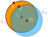
Figure 2: Illustration of the distillation hypothesis sets. Notice that the diameter of a hypothesis set ${\mathscr{H}}_{S}$ may be large here.

In the second stage, the algorithm selects a hypothesis that is $\gamma$-close to $f^{*}_{S}$ from a less complex family of predictors ${\mathscr{H}}$. This defines the following sample-dependent hypothesis set: ${\mathscr{H}}_{S}=\big{\{}h\in{\mathscr{H}}\colon\|(h-f^{*}_{S})\|_{\infty}\leq\gamma\big{\}}$.

Assume that the loss $\ell$ is $\mu$-Lipschitz with respect to its first argument and that ${\mathscr{H}}$ is a subset of a vector space. Let $S$ and $S^{\prime}$ be two samples differing by one point. Note, $f^{*}_{S}$ may not be in ${\mathscr{H}}$, but we will assume that $f^{*}_{S^{\prime}}-f^{*}_{S}$ is in ${\mathscr{H}}$. Let $h$ be in ${\mathscr{H}}_{S}$, then the hypothesis $h^{\prime}=h+f^{*}_{S^{\prime}}-f^{*}_{S}$ is in ${\mathscr{H}}_{S^{\prime}}$ since $\|h^{\prime}-f^{*}_{S^{\prime}}\|_{\infty}=\|h-f^{*}_{S}\|_{\infty}\leq\gamma$. Figure 2 illustrates the hypothesis sets. By the $\mu$-Lipschitzness of the loss, for any $z=(x,y)\in{\mathscr{Z}}$, $|\ell(h^{\prime}(x),y)-\ell(h(x),y)|\leq\mu\|h^{\prime}(x)-h(x)\|_{\infty}=\mu\|f^{*}_{S^{\prime}}-f^{*}_{S}\|\leq\mu\beta$. Thus, the family of hypothesis sets ${\mathscr{H}}_{S}$ is $\mu\beta$-stable.

In view of that, by Theorem 2, for any $\delta>0$, with probability at least $1-\delta$ over the draw of a sample $S\sim{\mathscr{D}}^{m}$, the following inequality holds for any $h\in{\mathscr{H}}_{S}$:

$$R(h)\leq\widehat{R}_{S}(h)+2\mathfrak{R}^{\diamond}_{m}(\mathcal{G})+(1+2\mu\beta m)\sqrt{\tfrac{1}{2m}\log(\tfrac{1}{\delta})}.$$

Notice that a standard uniform-stability argument would not necessarily apply here since ${\mathscr{H}}_{S}$ could be relatively complex and the second stage not necessarily stable.

6 Conclusion

We presented a broad study of generalization with data-dependent hypothesis sets, including general learning bounds using a notion of transductive Rademacher complexity and, more importantly, learning bounds for stable data-dependent hypothesis sets. We illustrated the applications of these guarantees to the analysis of several problems. Our framework is general and covers learning scenarios commonly arising in applications for which standard generalization bounds are not applicable. Our results can be further augmented and refined to include model selection bounds and local Rademacher complexity bounds for stable data-dependent hypothesis sets (to be presented in a more extended version of this manuscript), and further extensions described in Appendix F. Our analysis can also be extended to the non-i.i.d. setting and other learning scenarios such as that of transduction. Several by-products of our analysis, including our proof techniques, new guarantees for transductive learning, and our PAC-Bayesian bounds for randomized algorithms, both in the sample-independent and sample-dependent cases, can be of independent interest. While we highlighted several applications of our learning bounds, a tighter analysis might be needed to derive guarantees for a wider range of data-dependent hypothesis classes or scenarios.

Acknowledgements.

HL is supported by NSF IIS-1755781. The work of SG and MM was partly supported by NSF CCF-1535987, NSF IIS-1618662, and a Google Research Award. KS would like to acknowledge NSF CAREER Award 1750575 and Sloan Research Fellowship.

Appendix A Further background on stability

The study of stability dates back to early work on the analysis of $k$-neareast neighbor and other local discrimination rules [Rogers and Wagner, 1978, Devroye and Wagner, 1979]. Stability has been critically used in the analysis of stochastic optimization [Shalev-Shwartz et al., 2010] and online-to-batch conversion [Cesa-Bianchi et al., 2001]. Stability bounds have been generalized to the non-i.i.d. settings, including stationary [Mohri and Rostamizadeh, 2010] and non-stationary [Kuznetsov and Mohri, 2017] $\phi$-mixing and $\beta$-mixing processes. They have also been used to derive learning bounds for transductive inference [Cortes et al., 2008]. Stability bounds were further extended to cover almost stable algorithms by Kutin and Niyogi [2002]. These authors also discussed a number of alternative definitions of stability, see also [Kearns and Ron, 1997]. An alternative notion of stability was also used by Kale et al. [2011] to analyze $k$-fold cross-validation for a number of stable algorithms.

Appendix B Properties of data-dependent Rademacher complexity

In this section, we highlight several key properties of our notion of data-dependent Rademacher complexity.

B.1 Upper-bound on Rademacher complexity of data-dependent hypothesis sets

Lemma 2.

For any sample $S=(x^{S}_{1},\ldots,x^{S}_{m})\in\mathbb{R}^{N}$, define the hypothesis set ${\mathscr{H}}_{S}$ as follows:

$${\mathscr{H}}_{S}=\bigg{\{}x\mapsto w^{S}\cdot x\colon\ w^{S}=\sum_{i=1}^{m}\alpha_{i}x^{S}_{i},\|\alpha\|_{1}\leq\Lambda_{1}\bigg{\}},$$

where $\Lambda_{1}\geq 0$. Define $r_{T}$ and $r_{S\cup T}$ as follows: $r_{T}=\sqrt{\frac{\sum_{i=1}^{m}\|x^{T}_{i}\|_{2}^{2}}{m}}$ and $r_{S\cup T}=\max_{x\in S\cup T}\|x\|_{2}$. Then, the empirical Rademacher complexity of the family of data-dependent hypothesis sets $\mathcal{H}=({\mathscr{H}}_{S})_{S\in{\mathscr{X}}^{m}}$ can be upper-bounded as follows:

$$\widehat{\mathfrak{R}}^{\diamond}_{S,T}(\mathcal{H})\leq r_{T}\,r_{S\cup T}\Lambda_{1}\sqrt{\frac{2\log(4m)}{m}}\leq r^{2}_{S\cup T}\Lambda_{1}\sqrt{\frac{2\log(4m)}{m}}.$$

Proof.

The following inequalities hold:

$$\widehat{\mathfrak{R}}^{\diamond}_{S,T}(\mathcal{H})=\frac{1}{m}\operatorname*{\mathbb{E}}_{{\boldsymbol{\sigma}}}\bigg{[}\sup_{h\in{\mathscr{H}}_{S,T}^{\boldsymbol{\sigma}}}\sum_{i=1}^{m}\sigma_{i}h(x^{T}_{i})\bigg{]} =\frac{1}{m}\operatorname*{\mathbb{E}}_{{\boldsymbol{\sigma}}}\bigg{[}\sup_{\|\alpha\|_{1}\leq\Lambda_{1}}\sum_{i=1}^{m}\sigma_{i}\sum_{j=1}^{m}\alpha_{j}x^{S_{T,{\boldsymbol{\sigma}}}}_{j}\cdot x^{T}_{i}\bigg{]}$$

$$=\frac{1}{m}\operatorname*{\mathbb{E}}_{{\boldsymbol{\sigma}}}\bigg{[}\sup_{\|\alpha\|_{1}\leq\Lambda_{1}}\sum_{j=1}^{m}\alpha_{j}\left(x^{S_{T,{\boldsymbol{\sigma}}}}_{j}\sum_{i=1}^{m}\sigma_{i}\cdot x^{T}_{i}\right)\bigg{]}$$

$$=\frac{\Lambda_{1}}{m}\operatorname*{\mathbb{E}}_{{\boldsymbol{\sigma}}}\bigg{[}\max_{j\in[m]}\left|x^{S_{T,{\boldsymbol{\sigma}}}}_{j}\cdot\sum_{i=1}^{m}\sigma_{i}x^{T}_{i}\right|\bigg{]}$$

$$\leq\frac{\Lambda_{1}}{m}\operatorname*{\mathbb{E}}_{{\boldsymbol{\sigma}}}\bigg{[}\max_{\begin{subarray}{c}x^{\prime}\in S\cup T\\ \sigma^{\prime}\in\{-1,+1\}\end{subarray}}\sum_{i=1}^{m}\sigma_{i}(\sigma^{\prime}x^{\prime}\cdot x^{T}_{i})\bigg{]}.$$

The norm of the vector $z^{\prime}\in\mathbb{R}^{m}$ with coordinates $(\sigma^{\prime}x^{\prime}\cdot x^{T}_{i})$ can be bounded as follows:

$$\sqrt{\sum_{i=1}^{m}(\sigma^{\prime}x^{\prime}\cdot x^{T}_{i})^{2}}\leq\|x^{\prime}\|\sqrt{\sum_{i=1}^{m}\|x^{T}_{i}\|^{2}}\leq r_{S\cup T}\,\sqrt{m}\,r_{T}.$$

Thus, by Massart’s lemma, since $|S\cup T|\leq 2m$, the following inequality holds:

$$\widehat{\mathfrak{R}}^{\diamond}_{S,T}(\mathcal{H})\leq r_{T}\,r_{S\cup T}\Lambda_{1}\sqrt{\frac{2\log(4m)}{m}}\leq r^{2}_{S\cup T}\Lambda_{1}\sqrt{\frac{2\log(4m)}{m}},$$

which completes the proof. ∎

Notice that the bound on the Rademacher complexity in Lemma 2is non-trivial since it depends on the samples $S$ and $T$, while a standard Rademacher complexity for non-data-dependent hypothesis set containing ${\mathscr{H}}_{S}$ would require taking a maximum over all samples $S$ of size $m$.

Lemma 3.

Suppose ${\mathscr{X}}=\mathbb{R}^{N}$, and for every sample $S\in{\mathscr{Z}}^{m}$ we associate a matrix $A_{S}\in\mathbb{R}^{d\times N}$ for some $d>0$, and let $\mathcal{W}_{S,\Lambda}=\{w\in\mathbb{R}^{d}:\ \|A_{S}^{\top}w\|_{2}\leq\Lambda\}$ for some $\Lambda>0$. Consider the hypothesis set ${\mathscr{H}}_{S}:=\bigg{\{}x\mapsto w^{\top}A_{S}x\colon\ w\in\mathcal{W}_{S,\Lambda}\bigg{\}}$. Then, the empirical Rademacher complexity of the family of data-dependent hypothesis sets $\mathcal{H}=({\mathscr{H}}_{S})_{S\in{\mathscr{Z}}^{m}}$ can be upper-bounded as follows:

$$\widehat{\mathfrak{R}}^{\diamond}_{S,T}(\mathcal{H})\leq\frac{\Lambda\sqrt{\sum_{i=1}^{m}\|x^{T}_{i}\|_{2}^{2}}}{m}\leq\frac{\Lambda r}{\sqrt{m}},$$

where $r=\sup_{i\in[m]}\|x^{T}_{i}\|_{2}$.

Proof.

Let $X_{T}=[x^{T}_{1}\,\cdots\,x^{T}_{m}]$. The following inequalities hold:

$$\widehat{\mathfrak{R}}^{\diamond}_{S,T}(\mathcal{H})=\frac{1}{m}\operatorname*{\mathbb{E}}_{{\boldsymbol{\sigma}}}\bigg{[}\sup_{h\in{\mathscr{H}}_{S,T}^{\boldsymbol{\sigma}}}\sum_{i=1}^{m}\sigma_{i}h(x^{T}_{i})\bigg{]} =\frac{1}{m}\operatorname*{\mathbb{E}}_{{\boldsymbol{\sigma}}}\bigg{[}\sup_{w:\ \|A_{S}^{\top}w\|_{2}\leq\Lambda}w^{\top}A_{S}X_{T}{\boldsymbol{\sigma}}\bigg{]}$$

$$\leq\frac{\Lambda}{m}\operatorname*{\mathbb{E}}_{{\boldsymbol{\sigma}}}\big{[}\|X_{T}{\boldsymbol{\sigma}}\|_{2}\big{]} (\text{Cauchy-Schwarz})$$

$$\leq\frac{\Lambda}{m}\sqrt{\operatorname*{\mathbb{E}}_{{\boldsymbol{\sigma}}}\big{[}\|X_{T}{\boldsymbol{\sigma}}\|^{2}_{2}\big{]}} (\text{Jensen's ineq.})$$

$$\leq\frac{\Lambda}{m}\sqrt{\operatorname*{\mathbb{E}}_{{\boldsymbol{\sigma}}}\bigg{[}\sum_{i,j=1}^{m}\sigma_{i}\sigma_{j}(x^{T}_{i}\cdot x^{T}_{j})\bigg{]}}$$

$$=\frac{\Lambda\sqrt{\sum_{i=1}^{m}\|x^{T}_{i}\|_{2}^{2}}}{m},$$

which completes the proof. ∎

B.2 Concentration

Lemma 4.

Let $\mathcal{H}$ a family of $\beta$-stable data-dependent hypothesis sets. Then, for any $\delta>0$, with probability at least $1-\delta$ (over the draw of two samples $S$ and $T$ with size $m$), the following inequality holds:

$$\Big{|}\widehat{\mathfrak{R}}^{\diamond}_{S,T}(\mathcal{G})-\mathfrak{R}^{\diamond}_{m}(\mathcal{G})\Big{|}\leq\sqrt{\frac{[(m\beta+1)^{2}+m^{2}\beta^{2}]\log\frac{2}{\delta}}{2m}}.$$

Proof.

Let $T^{\prime}$ be a sample differing from $T$ only by point. Fix $\eta>0$. For any ${\boldsymbol{\sigma}}$, by definition of the supremum, there exists $h^{\prime}\in{\mathscr{H}}_{S,T^{\prime}}^{\boldsymbol{\sigma}}$ such that:

$$\sum_{i=1}^{m}\sigma_{i}L(h^{\prime},z^{T}_{i})\geq\sup_{h\in{\mathscr{H}}_{S,T^{\prime}}^{\boldsymbol{\sigma}}}\sum_{i=1}^{m}\sigma_{i}L(h,z^{T^{\prime}}_{i})-\eta.$$

By the $\beta$-stability of $\mathcal{H}$, there exists $h\in{\mathscr{H}}_{S,T}^{\boldsymbol{\sigma}}$ such that for any $z\in{\mathscr{Z}}$, $|L(h^{\prime},z)-L(h,z)|\leq\beta$. Thus, we have

$$\sup_{h\in{\mathscr{H}}_{S,T^{\prime}}^{\boldsymbol{\sigma}}}\sum_{i=1}^{m}\sigma_{i}L(h,z^{T^{\prime}}_{i})\leq\sum_{i=1}^{m}\sigma_{i}L(h^{\prime},z^{T^{\prime}}_{i})+\eta\leq\sum_{i=1}^{m}[\sigma_{i}(L(h,z^{T^{\prime}}_{i})+\beta)]+\eta.$$

Since the inequality holds for all $\eta>0$, we have

$$\frac{1}{m}\sup_{h\in{\mathscr{H}}_{S,T^{\prime}}^{\boldsymbol{\sigma}}}\sum_{i=1}^{m}\sigma_{i}L(h,z^{T^{\prime}}_{i})\leq\frac{1}{m}\sum_{i=1}^{m}\sigma_{i}(L(h,z^{T^{\prime}}_{i})+\beta)\leq\frac{1}{m}\sup_{h\in{\mathscr{H}}_{S,T}^{\boldsymbol{\sigma}}}\sum_{i=1}^{m}\sigma_{i}L(h,z^{T}_{i})+\beta+\frac{1}{m}.$$

Thus, replacing $T$ by $T^{\prime}$ affects $\widehat{\mathfrak{R}}^{\diamond}_{S,T}(\mathcal{G})$ by at most $\beta+\frac{1}{m}$. By the same argument, changing sample $S$ by one point modifies $\widehat{\mathfrak{R}}^{\diamond}_{S,T}(\mathcal{G})$ at most by $\beta$. Thus, by McDiarmid’s inequality, for any $\delta>0$, with probability at least $1-\delta$, the following inequality holds:

$$\Big{|}\widehat{\mathfrak{R}}^{\diamond}_{S,T}(\mathcal{G})-\mathfrak{R}^{\diamond}_{m}(\mathcal{G})\Big{|}\leq\sqrt{\frac{[(m\beta+1)^{2}+m^{2}\beta^{2}]\log\frac{2}{\delta}}{2m}}.$$

This completes the proof. ∎

Appendix C Proof of Lemma 1

Proof.

Let $S\in{\mathscr{Z}}^{m}$, $z\in S$, and $z^{\prime}\in{\mathscr{Z}}$. For any $h\in{\mathscr{H}}_{S}$ and $h^{\prime}\in{\mathscr{H}}_{S^{z\leftrightarrow z^{\prime}}}$, by the $\beta$-uniform stability of $\mathcal{H}$, there exists $h^{\prime\prime}\in{\mathscr{H}}_{S}$ such that $L(h^{\prime},z)-L(h^{\prime\prime},z)\leq\beta$. Thus,

$$L(h^{\prime},z)-L(h,z)=L(h^{\prime},z)-L(h^{\prime\prime},z)+L(h^{\prime\prime},z)-L(h,z)\leq\beta+\sup_{h^{\prime\prime}\!,\,h\in{\mathscr{H}}_{S}}L(h^{\prime\prime},z)-L(h,z).$$

This implies the inequality

$$\sup_{h\in{\mathscr{H}}_{S},h^{\prime}\in{\mathscr{H}}_{S^{z\leftrightarrow z^{\prime}}}}L(h^{\prime},z)-L(h,z)\leq\beta+\sup_{h^{\prime\prime}\!,\,h\in{\mathscr{H}}_{S}}L(h^{\prime\prime},z)-L(h,z),$$

and the lemma follows. ∎

Appendix D Proof of Theorem 1

In this section, we present the proof of Theorem 1.

Proof.

We will use the following symmetrization result, which holds for any $\epsilon>0$ with $n\epsilon^{2}\geq 2$ for data-dependent hypothesis sets (Lemma 5 below):

$$\operatorname*{\mathbb{P}}_{S\sim{\mathscr{D}}^{m}}\bigg{[}\sup_{h\in{\mathscr{H}}_{S}}R(h)-\widehat{R}_{S}(h)>\epsilon\bigg{]}\leq 2\operatorname*{\mathbb{P}}_{\begin{subarray}{c}S\sim{\mathscr{D}}^{m}\\ T\sim{\mathscr{D}}^{n}\mspace{6.0mu}\end{subarray}}\bigg{[}\sup_{h\in{\mathscr{H}}_{S}}\widehat{R}_{T}(h)-\widehat{R}_{S}(h)>\frac{\epsilon}{2}\bigg{]}.$$ (13)

Thus, we will seek to bound the right-hand side as follows, where we write $(S,T)\sim U$ to indicate that the sample $S$ of size $m$ is drawn uniformly without replacement from $U$ and that $T$ is the remaining part of $U$, that is $(S,T)=U$:

$$\operatorname*{\mathbb{P}}_{\begin{subarray}{c}S\sim{\mathscr{D}}^{m}\\ T\sim{\mathscr{D}}^{n}\mspace{6.0mu}\end{subarray}}\bigg{[}\sup_{h\in{\mathscr{H}}_{S}}\widehat{R}_{T}(h)-\widehat{R}_{S}(h)>\frac{\epsilon}{2}\bigg{]}$$

$$=\operatorname*{\mathbb{E}}_{U\sim{\mathscr{D}}^{m+n}}\Bigg{[}\operatorname*{\mathbb{P}}_{\begin{subarray}{c}(S,T)\sim U\\ |S|=m,|T|=n\end{subarray}}\bigg{[}\sup_{h\in{\mathscr{H}}_{S}}\widehat{R}_{T}(h)-\widehat{R}_{S}(h)>\frac{\epsilon}{2}\bigg{]}\ \bigg{\mid}\ U\Bigg{]}$$

$$\leq\operatorname*{\mathbb{E}}_{U\sim{\mathscr{D}}^{m+n}}\Bigg{[}\operatorname*{\mathbb{P}}_{\begin{subarray}{c}(S,T)\sim U\\ |S|=m,|T|=n\end{subarray}}\bigg{[}\sup_{h\in\overline{\mathscr{H}}_{U,m}}\widehat{R}_{T}(h)-\widehat{R}_{S}(h)>\frac{\epsilon}{2}\bigg{]}\ \bigg{\mid}\ U\Bigg{]}.$$

To upper bound the probability inside the expectation, we use an extension of McDiarmid’s inequality to sampling without replacement [Cortes et al., 2008], which applies to symmetric functions. We can apply that extension to $\Phi(S)=\sup_{h\in\overline{\mathscr{H}}_{U,m}}\widehat{R}_{T}(h)-\widehat{R}_{S}(h)$, for a fixed $U$, since $\Phi(S)$ is a symmetric function of the sample points $z_{1},\ldots,z_{m}$ in $S$. Changing one point in $S$ affects $\Phi(S)$ at most by $\frac{1}{m}+\frac{1}{m}=\frac{m+u}{mu}$, thus, by the extension of McDiarmid’s inequality to sampling without replacement, for a fixed $U\in{\mathscr{Z}}^{m+n}$, the following inequality holds:

$$\operatorname*{\mathbb{P}}_{\begin{subarray}{c}(S,T)\sim U\\ |S|=m,|T|=n\end{subarray}}\bigg{[}\sup_{h\in\overline{\mathscr{H}}_{U,m}}\widehat{R}_{T}(h)-\widehat{R}_{S}(h)>\frac{\epsilon}{2}\bigg{]}\leq\exp\bigg{[}-\frac{2}{\eta}\frac{mn}{m+n}\bigg{(}\frac{\epsilon}{2}-\operatorname*{\mathbb{E}}[\Phi(S)]\bigg{)}^{2}\bigg{]},$$ (14)

where $\eta=\frac{m+n}{m+n-\frac{1}{2}}\frac{1}{1-\frac{1}{2\max\{m,n\}}}\leq 3$. Plugging in the bound on $\operatorname*{\mathbb{E}}[\Phi(S)]$ of Lemma 6 below, and setting

$$\epsilon=\max_{U\in{\mathscr{Z}}^{m+n}}2\widehat{\mathfrak{R}}^{\diamond}_{U,m}(\mathcal{G})+3\sqrt{\left(\tfrac{1}{m}+\tfrac{1}{n}\right)\log(\tfrac{2}{\delta})}+2\sqrt{\left(\tfrac{1}{m}+\tfrac{1}{n}\right)^{3}mn},$$

which satisfies $n\epsilon^{2}\geq 2$, it is easy to check that the RHS in (14) becomes smaller than $\frac{\delta}{2}$. This in turn implies, via (13), that the probability that $\sup_{h\in{\mathscr{H}}_{S}}R(h)-\widehat{R}_{S}(h)>\epsilon$ is at most $\delta$, completing the proof. ∎

The following lemma shows that the standard symmetrization lemma holds for data-dependent hypothesis sets. This observation was already made by Gat [2001] (see also Lemma 2 in [Cannon et al., 2002]) for the symmetrization lemma of Vapnik [1998][p. 139], used by the author in the case $n=m$. However, that symmetrization lemma of Vapnik [1998] holds only for random variables taking values in $\{0,1\}$ and its proof is not complete since the hypergeometric inequality is not proven.

Lemma 5.

Let $n\geq 1$ and fix $\epsilon>0$ such that $n\epsilon^{2}\geq 2$. Then, the following inequality holds:

$$\operatorname*{\mathbb{P}}_{S\sim{\mathscr{D}}^{m}}\bigg{[}\sup_{h\in{\mathscr{H}}_{S}}R(h)-\widehat{R}_{S}(h)>\epsilon\bigg{]}\leq 2\operatorname*{\mathbb{P}}_{\begin{subarray}{c}S\sim{\mathscr{D}}^{m}\\ T\sim{\mathscr{D}}^{n}\mspace{6.0mu}\end{subarray}}\bigg{[}\sup_{h\in{\mathscr{H}}_{S}}\widehat{R}_{T}(h_{S})-\widehat{R}_{S}(h_{S})>\frac{\epsilon}{2}\bigg{]}.$$

Proof.

The proof is standard. Below, we are giving a concise version mainly for the purpose of verifying that the data-dependency of the hypothesis set does not affect its correctness.

Fix $\eta>0$. By definition of the supremum, there exists $h_{S}\in{\mathscr{H}}_{S}$ such that

$$\sup_{h\in{\mathscr{H}}_{S}}R(h)-\widehat{R}_{S}(h)-\eta\leq R(h_{S})-\widehat{R}_{S}(h_{S}).$$

Since $\widehat{R}_{T}(h_{S})-\widehat{R}_{S}(h_{S})=\widehat{R}_{T}(h_{S})-R(h_{S})+R(h_{S})-\widehat{R}_{S}(h_{S})$, we can write

$$1_{\widehat{R}_{T}(h_{S})-\widehat{R}_{S}(h_{S})>\frac{\epsilon}{2}} \geq 1_{\widehat{R}_{T}(h_{S})-R(h_{S})>-\frac{\epsilon}{2}}1_{R(h_{S})-\widehat{R}_{S}(h_{S})>\epsilon}=1_{R(h_{S})-\widehat{R}_{T}(h_{S})<\frac{\epsilon}{2}}1_{R(h_{S})-\widehat{R}_{S}(h_{S})>\epsilon}.$$

Thus, for any $S\in{\mathscr{Z}}^{m}$, taking the expectation of both sides with respect to $T$ yields

$$\operatorname*{\mathbb{P}}_{T\sim{\mathscr{D}}^{n}}\bigg{[}\widehat{R}_{T}(h_{S})-\widehat{R}_{S}(h_{S})>\frac{\epsilon}{2}\bigg{]} \geq\operatorname*{\mathbb{P}}_{T\sim{\mathscr{D}}^{n}}\bigg{[}R(h_{S})-\widehat{R}_{T}(h_{S})<\frac{\epsilon}{2}\bigg{]}\ 1_{R(h_{S})-\widehat{R}_{S}(h_{S})>\epsilon}$$

$$=\bigg{[}1-\operatorname*{\mathbb{P}}_{T\sim{\mathscr{D}}^{n}}\bigg{[}R(h_{S})-\widehat{R}_{T}(h_{S})\geq\frac{\epsilon}{2}\bigg{]}\bigg{]}\ 1_{R(h_{S})-\widehat{R}_{S}(h_{S})>\epsilon}$$

$$\leq\bigg{[}1-\frac{4\operatorname{Var}[L(h_{S},z)]}{n\epsilon^{2}}\bigg{]}\ 1_{R(h_{S})-\widehat{R}_{S}(h_{S})>\epsilon}$$ (Chebyshev’s ineq.)

$$\geq\bigg{[}1-\frac{1}{n\epsilon^{2}}\bigg{]}\ 1_{R(h_{S})-\widehat{R}_{S}(h_{S})>\epsilon}\ ,$$

where the last inequality holds since $L(h_{S},z)$ takes values in $[0,1]$:

$$\operatorname{Var}[L(h_{S},z)]=\operatorname*{\mathbb{E}}_{z\sim{\mathscr{D}}}[L^{2}(h_{S},z)]-\operatorname*{\mathbb{E}}_{z\sim{\mathscr{D}}}[L(h_{S},z)]^{2} \leq\operatorname*{\mathbb{E}}_{z\sim{\mathscr{D}}}[L(h_{S},z)]-\operatorname*{\mathbb{E}}_{z\sim{\mathscr{D}}}[L(h_{S},z)]^{2}$$

$$=\operatorname*{\mathbb{E}}_{z\sim{\mathscr{D}}}[L(h_{S},z)](1-\operatorname*{\mathbb{E}}_{z\sim{\mathscr{D}}}[L(h_{S},z)])\leq\frac{1}{4}.$$

Taking expectation with respect to $S$ gives

$$\operatorname*{\mathbb{P}}_{\begin{subarray}{c}S\sim{\mathscr{D}}^{m}\\ T\sim{\mathscr{D}}^{n}\mspace{6.0mu}\end{subarray}}\bigg{[}\widehat{R}_{T}(h_{S})-\widehat{R}_{S}(h_{S})>\frac{\epsilon}{2}\bigg{]} \geq\bigg{[}1-\frac{1}{n\epsilon^{2}}\bigg{]}\operatorname*{\mathbb{P}}_{S\sim{\mathscr{D}}^{m}}\bigg{[}R(h_{S})-\widehat{R}_{S}(h_{S})>\epsilon\bigg{]}$$

$$\geq\frac{1}{2}\operatorname*{\mathbb{P}}_{S\sim{\mathscr{D}}^{m}}\bigg{[}R(h_{S})-\widehat{R}_{S}(h_{S})>\epsilon\bigg{]} (n\epsilon^{2}\geq 2)$$

$$\geq\frac{1}{2}\operatorname*{\mathbb{P}}_{S\sim{\mathscr{D}}^{m}}\bigg{[}\sup_{h\in{\mathscr{H}}_{S}}R(h)-\widehat{R}_{S}(h)>\epsilon+\eta\bigg{]}.$$

Since the inequality holds for all $\eta>0$, by the right-continuity of the cumulative distribution function, it implies

$$\operatorname*{\mathbb{P}}_{\begin{subarray}{c}S\sim{\mathscr{D}}^{m}\\ T\sim{\mathscr{D}}^{n}\mspace{6.0mu}\end{subarray}}\bigg{[}\widehat{R}_{T}(h_{S})-\widehat{R}_{S}(h_{S})>\frac{\epsilon}{2}\bigg{]}\geq\frac{1}{2}\operatorname*{\mathbb{P}}_{S\sim{\mathscr{D}}^{m}}\bigg{[}\sup_{h\in{\mathscr{H}}_{S}}R(h)-\widehat{R}_{S}(h)>\epsilon\bigg{]}.$$

Since $h_{S}$ is in ${\mathscr{H}}_{S}$, by definition of the supremum, we have

$$\operatorname*{\mathbb{P}}_{\begin{subarray}{c}S\sim{\mathscr{D}}^{m}\\ T\sim{\mathscr{D}}^{n}\mspace{6.0mu}\end{subarray}}\bigg{[}\sup_{h\in{\mathscr{H}}_{S}}\widehat{R}_{T}(h)-\widehat{R}_{S}(h)>\frac{\epsilon}{2}\bigg{]}\geq\operatorname*{\mathbb{P}}_{\begin{subarray}{c}S\sim{\mathscr{D}}^{m}\\ T\sim{\mathscr{D}}^{n}\mspace{6.0mu}\end{subarray}}\bigg{[}\widehat{R}_{T}(h_{S})-\widehat{R}_{S}(h_{S})>\frac{\epsilon}{2}\bigg{]},$$

which completes the proof. ∎

The following lemma provides a bound on $\operatorname*{\mathbb{E}}[\Phi(S)]$:

Lemma 6.

Fix $U\in{\mathscr{Z}}^{m+n}$. Then, the following upper bound holds:

$$\operatorname*{\mathbb{E}}_{\begin{subarray}{c}(S,T)\sim U\\ |S|=m,|T|=n\end{subarray}}\bigg{[}\sup_{h\in\overline{\mathscr{H}}_{U,m}}\widehat{R}_{T}(h)-\widehat{R}_{S}(h)\bigg{]}\leq\widehat{\mathfrak{R}}^{\diamond}_{U,m}(\mathcal{G})+\sqrt{\frac{\log(2e)(m+n)^{3}}{2(mn)^{2}}}.$$

For $m=n$, the inequality becomes:

$$\operatorname*{\mathbb{E}}_{\begin{subarray}{c}(S,T)\sim U\\ |S|=m,|T|=n\end{subarray}}\bigg{[}\sup_{h\in\overline{\mathscr{H}}_{U,m}}\widehat{R}_{T}(h)-\widehat{R}_{S}(h)\bigg{]}\leq\widehat{\mathfrak{R}}^{\diamond}_{U,m}(\mathcal{G})+2\sqrt{\frac{\log(2e)}{m}}.$$

Proof.

The proof is an extension of the analysis of maximum discrepancy in [Bartlett and Mendelson, 2002]. Let $|{\boldsymbol{\sigma}}|$ denote $\sum_{i=1}^{m+n}\sigma_{i}$ and let $I\subseteq\Big{[}\mspace{-6.0mu}-\frac{(m+n)^{2}}{m},\frac{(m+n)^{2}}{n}\Big{]}$ denote the set of values $|{\boldsymbol{\sigma}}|$ can take. For any $q\in I$, define $s(q)$ as follows:

$$s(q)=\operatorname*{\mathbb{E}}_{\boldsymbol{\sigma}}\bigg{[}\sup_{h\in\overline{\mathscr{H}}_{U,m}}\frac{1}{m+n}\sum_{i=1}^{m+n}\sigma_{i}L(h,z^{U}_{i})\bigg{|}\,|{\boldsymbol{\sigma}}|=q\bigg{]}.$$

Let $|{\boldsymbol{\sigma}}|_{+}$ denote the number of positive $\sigma_{i}$s, taking value $\frac{m+n}{n}$, then $|{\boldsymbol{\sigma}}|$ can be expressed as follows:

$$|{\boldsymbol{\sigma}}|=\sum_{i=1}^{m+n}\sigma_{i}=|{\boldsymbol{\sigma}}|_{+}\frac{m+n}{n}-(m+n-|{\boldsymbol{\sigma}}|_{+})\frac{m+n}{m}=\frac{(m+n)^{2}}{mn}(|{\boldsymbol{\sigma}}|_{+}-n).$$ (15)

Thus, we have $|{\boldsymbol{\sigma}}|=0$ iff $|{\boldsymbol{\sigma}}|_{+}=m$, and the condition ($|{\boldsymbol{\sigma}}|=0$) precisely corresponds to having the equality

$$\frac{1}{m+n}\sum_{i=1}^{m+n}\sigma_{i}L(h,z^{U}_{i})=\widehat{R}_{T}(h)-\widehat{R}_{S}(h),$$

where $S$ is the sample of size $m$ defined by those $z_{i}$s for which $\sigma_{i}$ takes value $\frac{m+n}{n}$. In view of that, we have

$$\operatorname*{\mathbb{E}}_{\begin{subarray}{c}(S,T)\sim U\\ |S|=m,|T|=n\end{subarray}}\bigg{[}\sup_{h\in\overline{\mathscr{H}}_{U,m}}\widehat{R}_{T}(h)-\widehat{R}_{S}(h)\bigg{]}=s(0).$$

Let $q_{1},q_{2}\in I$, with $q_{1}=p_{1}\frac{m+n}{n}-(m+n-p_{1})\frac{m+n}{m}$, $q_{2}=p_{2}\frac{m+n}{n}-(m+n-p_{2})\frac{m+n}{m}$ and $q_{1}\leq q_{2}$. Then, we can write

$$s(q_{1}) =\operatorname*{\mathbb{E}}\left[\sup_{g\in G}\sum_{i=1}^{p_{1}}\frac{1}{n}L(h,z_{i})-\sum_{i=p_{1}+1}^{m+n}\frac{1}{m}L(h,z_{i})\right]$$

$$s(q_{2}) =\operatorname*{\mathbb{E}}\Bigg{[}\sup_{g\in G}\sum_{i=1}^{p_{1}}\frac{1}{n}L(h,z_{i})-\sum_{i=p_{1}+1}^{m+n}\frac{1}{m}L(h,z_{i})+\sum_{i=p_{1}+1}^{p_{2}}\left[\frac{1}{n}+\frac{1}{m}\right]L(h,z_{i})\Bigg{]}.$$

Thus, we have the following Lipschitz property:

$$|s(q_{2})-s(q_{1})|\leq|p_{2}-p_{1}|\bigg{[}\frac{1}{m}+\frac{1}{n}\bigg{]} =|(p_{2}-n)-(p_{1}-n)|\bigg{[}\frac{1}{m}+\frac{1}{n}\bigg{]}$$ (using (15))

$$=|q_{2}-q_{1}|\frac{mn}{(m+n)^{2}}\bigg{[}\frac{1}{m}+\frac{1}{n}\bigg{]}$$

$$=\frac{|q_{2}-q_{1}|}{m+n}.$$

By this Lipschitz property, we can write

$$\operatorname*{\mathbb{P}}\Big{[}\big{|}s(|{\boldsymbol{\sigma}}|)-s(\operatorname*{\mathbb{E}}[|{\boldsymbol{\sigma}}|])\big{|}>\epsilon\Big{]}\leq\operatorname*{\mathbb{P}}\Big{[}\big{|}|{\boldsymbol{\sigma}}|-\operatorname*{\mathbb{E}}[|{\boldsymbol{\sigma}}|]\big{|}>(m+n)\epsilon\Big{]}\leq 2\exp\bigg{[}-2\frac{(mn)^{2}\epsilon^{2}}{(m+n)^{3}}\bigg{]},$$

since the range of each $\sigma_{i}$ is $\frac{m+n}{n}+\frac{m+n}{m}=\frac{(m+n)^{2}}{mn}$. We now use this inequality to bound the second moment of $Z=s(|{\boldsymbol{\sigma}}|)-s(\operatorname*{\mathbb{E}}[|{\boldsymbol{\sigma}}|])=s(|{\boldsymbol{\sigma}}|)-s(0)$, as follows, for any $u\geq 0$:

$$\operatorname*{\mathbb{E}}[Z^{2}] =\int_{0}^{+\infty}\operatorname*{\mathbb{P}}[Z^{2}>t]\,dt$$

$$=\int_{0}^{u}\operatorname*{\mathbb{P}}[Z^{2}>t]\,dt+\int_{u}^{+\infty}\operatorname*{\mathbb{P}}[Z^{2}>t]\,dt$$

$$\leq u+2\int_{u}^{+\infty}\exp\bigg{[}-2\frac{(mn)^{2}t}{(m+n)^{3}}\bigg{]}\,dt$$

$$\leq u+\bigg{[}\frac{(m+n)^{3}}{(mn)^{2}}\exp\bigg{[}-2\frac{(mn)^{2}t}{(m+n)^{3}}\bigg{]}\bigg{]}_{u}^{+\infty}$$

$$=u+\frac{(m+n)^{3}}{(mn)^{2}}\exp\bigg{[}-2\frac{(mn)^{2}u}{(m+n)^{3}}\bigg{]}.$$

Choosing $u=\frac{1}{2}\frac{\log(2)(m+n)^{3}}{(mn)^{2}}$ to minimize the right-hand side gives $\operatorname*{\mathbb{E}}[Z^{2}]\leq\frac{\log(2e)(m+n)^{3}}{2(mn)^{2}}$. By Jensen’s inequality, this implies $\operatorname*{\mathbb{E}}[|Z|]\leq\sqrt{\frac{\log(2e)(m+n)^{3}}{2(mn)^{2}}}$ and therefore

$$\operatorname*{\mathbb{E}}_{\begin{subarray}{c}(S,T)\sim U\\ |S|=m,|T|=n\end{subarray}}\bigg{[}\sup_{h\in\overline{\mathscr{H}}_{U,m}}\widehat{R}_{T}(h)-\widehat{R}_{S}(h)\bigg{]}=s(0)\leq\operatorname*{\mathbb{E}}[s(|{\boldsymbol{\sigma}}|)]+\sqrt{\frac{\log(2e)(m+n)^{3}}{2(mn)^{2}}}.$$

Since we have $\operatorname*{\mathbb{E}}[s(|{\boldsymbol{\sigma}}|)]=\widehat{\mathfrak{R}}_{U,m}^{\diamond}(\mathcal{G})$, this completes the proof. ∎

Appendix E Proof of Theorem 2

In this section, we present the full proof of Theorem 2. The proof of each of the three bounds (9), (10) and (11) are given in separate subsections.

E.1 Proof of bound (9)

Proof.

For any two samples $S,S^{\prime}$, define the $\Psi(S,S^{\prime})$ as follows:

$$\Psi(S,S^{\prime})=\sup_{h\in{\mathscr{H}}_{S}}R(h)-\widehat{R}_{S^{\prime}}(h).$$

The proof consists of applying McDiarmid’s inequality to $\Psi(S,S)$. For any sample $S^{\prime}$ differing from $S$ by one point, we can decompose $\Psi(S,S)-\Psi(S^{\prime},S^{\prime})$ as follows:

$$\Psi(S,S)-\Psi(S^{\prime},S^{\prime})=\big{[}\Psi(S,S)-\Psi(S,S^{\prime})\big{]}+\big{[}\Psi(S,S^{\prime})-\Psi(S^{\prime},S^{\prime})\big{]}.$$

Now, by the sub-additivity of the $\sup$ operation, the first term can be upper-bounded as follows:

$$\Psi(S,S)-\Psi(S,S^{\prime}) \leq\sup_{h\in{\mathscr{H}}_{S}}\big{[}R(h)-\widehat{R}_{S}(h)\big{]}-\big{[}R(h)-\widehat{R}_{S^{\prime}}(h)\big{]}$$

$$\leq\sup_{h\in{\mathscr{H}}_{S}}\frac{1}{m}\big{[}L(h,z)-L(h,z^{\prime})\big{]}\leq\frac{1}{m},$$

where we denoted by $z$ and $z^{\prime}$ the labeled points differing in $S$ and $S^{\prime}$ and used the $1$-boundedness of the loss function.

We now analyze the second term:

$$\Psi(S,S^{\prime})-\Psi(S^{\prime},S^{\prime}) =\sup_{h\in{\mathscr{H}}_{S}}\big{[}R(h)-\widehat{R}_{S^{\prime}}(h)\big{]}-\sup_{h\in{\mathscr{H}}_{S^{\prime}}}\big{[}R(h)-\widehat{R}_{S^{\prime}}(h)\big{]}.$$

By definition of the supremum, for any $\epsilon>0$, there exists $h\in{\mathscr{H}}_{S}$ such that

$$\sup_{h\in{\mathscr{H}}_{S}}\big{[}R(h)-\widehat{R}_{S^{\prime}}(h)\big{]}-\epsilon\leq\big{[}R(h)-\widehat{R}_{S^{\prime}}(h)\big{]}$$

By the $\beta$-stability of $(H_{S})_{S\in{\mathscr{Z}}^{m}}$, there exists $h^{\prime}\in{\mathscr{H}}_{S^{\prime}}$ such that for all $z$, $|L(h,z)-L(h^{\prime},z)|\leq\beta$. In view of these inequalities, we can write

$$\Psi(S,S^{\prime})-\Psi(S^{\prime},S^{\prime}) \leq\big{[}R(h)-\widehat{R}_{S^{\prime}}(h)\big{]}+\epsilon-\sup_{h\in{\mathscr{H}}_{S^{\prime}}}\big{[}R(h)-\widehat{R}_{S^{\prime}}(h)\big{]}$$

$$\leq\big{[}R(h)-\widehat{R}_{S^{\prime}}(h)\big{]}+\epsilon-\big{[}R(h^{\prime})-\widehat{R}_{S^{\prime}}(h^{\prime})\big{]}$$

$$\leq\big{[}R(h)-R(h^{\prime})\big{]}+\epsilon+\big{[}\widehat{R}_{S^{\prime}}(h^{\prime})-\widehat{R}_{S^{\prime}}(h)\big{]}$$

$$\leq\epsilon+2\beta.$$

Since the inequality holds for any $\epsilon>0$, it implies that $\Psi(S,S^{\prime})-\Psi(S^{\prime},S^{\prime})\leq 2\beta$. Summing up the bounds on the two terms shows the following:

$$\Psi(S,S)-\Psi(S^{\prime},S^{\prime})\leq\frac{1}{m}+2\beta.$$

Thus, by McDiarmid’s inequality, for any $\delta>0$, with probability at least $1-\delta$, we have

$$\Psi(S,S)\leq\operatorname*{\mathbb{E}}[\Psi(S,S)]+(1+2\beta m)\sqrt{\tfrac{1}{2m}\log(\tfrac{1}{\delta})}.$$ (16)

We now bound $\operatorname*{\mathbb{E}}[\Psi(S,S)]$ by $2\mathfrak{R}^{\diamond}_{m}(\mathcal{G})$ as follows:

$$\operatorname*{\mathbb{E}}_{S\sim{\mathscr{D}}^{m}}[\Psi(S,S)]$$

$$=\operatorname*{\mathbb{E}}_{S\sim{\mathscr{D}}^{m}}\bigg{[}\sup_{h\in{\mathscr{H}}_{S}}\big{[}R(h)-\widehat{R}_{S}(h)\big{]}\bigg{]}$$

$$=\operatorname*{\mathbb{E}}_{S\sim{\mathscr{D}}^{m}}\bigg{[}\sup_{h\in{\mathscr{H}}_{S}}\Big{[}\operatorname*{\mathbb{E}}_{T\sim{\mathscr{D}}^{m}}\big{[}\widehat{R}_{T}(h)\big{]}-\widehat{R}_{S}(h)\Big{]}\bigg{]} R(h)$$ (def. of )

$$\leq\operatorname*{\mathbb{E}}_{S,T\sim{\mathscr{D}}^{m}}\bigg{[}\sup_{h\in{\mathscr{H}}_{S}}\widehat{R}_{T}(h)-\widehat{R}_{S}(h)\bigg{]} \sup$$ (sub-additivity of )

$$=\operatorname*{\mathbb{E}}_{S,T\sim{\mathscr{D}}^{m}}\bigg{[}\sup_{h\in{\mathscr{H}}_{S}}\frac{1}{m}\sum_{i=1}^{m}\Big{[}L(h,z^{T}_{i})-L(h,z^{S}_{i})\Big{]}\bigg{]}$$

$$=\operatorname*{\mathbb{E}}_{S,T\sim{\mathscr{D}}^{m}}\bigg{[}\operatorname*{\mathbb{E}}_{\boldsymbol{\sigma}}\bigg{[}\sup_{h\in{\mathscr{H}}^{\boldsymbol{\sigma}}_{S,T}}\frac{1}{m}\sum_{i=1}^{m}\sigma_{i}\Big{[}L(h,z^{T}_{i})-L(h,z^{S}_{i})\Big{]}\bigg{]}\bigg{]}$$ (symmetry)

$$\leq\operatorname*{\mathbb{E}}_{\begin{subarray}{c}S,T\sim{\mathscr{D}}^{m}\\ {\boldsymbol{\sigma}}\end{subarray}}\bigg{[}\sup_{h\in{\mathscr{H}}^{\boldsymbol{\sigma}}_{S,T}}\frac{1}{m}\sum_{i=1}^{m}\sigma_{i}L(h,z^{T}_{i})+\sup_{h\in{\mathscr{H}}^{\boldsymbol{\sigma}}_{S,T}}\frac{1}{m}\sum_{i=1}^{m}-\sigma_{i}L(h,z^{S}_{i})\bigg{]} \sup$$ (sub-additivity of )

$$=\operatorname*{\mathbb{E}}_{\begin{subarray}{c}S,T\sim{\mathscr{D}}^{m}\\ {\boldsymbol{\sigma}}\end{subarray}}\bigg{[}\sup_{h\in{\mathscr{H}}^{\boldsymbol{\sigma}}_{S,T}}\frac{1}{m}\sum_{i=1}^{m}\sigma_{i}L(h,z^{T}_{i})+\sup_{h\in{\mathscr{H}}^{-{\boldsymbol{\sigma}}}_{T,S}}\frac{1}{m}\sum_{i=1}^{m}-\sigma_{i}L(h,z^{S}_{i})\bigg{]} ({\mathscr{H}}^{\boldsymbol{\sigma}}_{S,T}={\mathscr{H}}^{-{\boldsymbol{\sigma}}}_{T,S})$$

$$=\operatorname*{\mathbb{E}}_{\begin{subarray}{c}S,T\sim{\mathscr{D}}^{m}\\ {\boldsymbol{\sigma}}\end{subarray}}\bigg{[}\sup_{h\in{\mathscr{H}}^{\boldsymbol{\sigma}}_{S,T}}\frac{1}{m}\sum_{i=1}^{m}\sigma_{i}L(h,z^{T}_{i})+\sup_{h\in{\mathscr{H}}^{{\boldsymbol{\sigma}}}_{T,S}}\frac{1}{m}\sum_{i=1}^{m}\sigma_{i}L(h,z^{S}_{i})\bigg{]}$$ (symmetry)

$$=2\mathfrak{R}^{\diamond}_{m}(\mathcal{G}).$$ (linearity of expectation)

Now, we show that $\operatorname*{\mathbb{E}}_{S\sim{\mathscr{D}}^{m}}[\Psi(S,S)]\leq\bar{\chi}$. To do so, first fix $\epsilon>0$. By definition of the supremum, for any $S\in{\mathscr{Z}}^{m}$, there exists $h_{S}$ such that the following inequality holds:

$$\sup_{h\in{\mathscr{H}}_{S}}\big{[}R(h)-\widehat{R}_{S}(h)\big{]}-\epsilon\leq R(h_{S})-\widehat{R}_{S}(h_{S}).$$

Now, by definition of $R(h_{S})$, we can write

$$\operatorname*{\mathbb{E}}_{S\sim{\mathscr{D}}^{m}}\big{[}R(h_{S})\big{]}=\operatorname*{\mathbb{E}}_{S\sim{\mathscr{D}}^{m}}\bigg{[}\operatorname*{\mathbb{E}}_{z\sim{\mathscr{D}}}(L(h_{S},z)\bigg{]}=\operatorname*{\mathbb{E}}_{\begin{subarray}{c}S\sim{\mathscr{D}}^{m}\\ z\sim{\mathscr{D}}\mspace{14.0mu}\end{subarray}}\big{[}L(h_{S},z)\big{]}.$$

Then, by the linearity of expectation, we can also write

$$\operatorname*{\mathbb{E}}_{S\sim{\mathscr{D}}^{m}}\big{[}\widehat{R}_{S}(h_{S})\big{]}=\operatorname*{\mathbb{E}}_{\begin{subarray}{c}S\sim{\mathscr{D}}^{m}\\ z\sim S\end{subarray}}\big{[}L(h_{S},z)\big{]}=\operatorname*{\mathbb{E}}_{\begin{subarray}{c}S\sim{\mathscr{D}}^{m}\\ z^{\prime}\sim{\mathscr{D}}\mspace{14.0mu}\\ z\sim S\end{subarray}}\big{[}L(h_{S^{z\leftrightarrow z^{\prime}}},z^{\prime})\big{]}.$$

In view of these two equalities, we can now rewrite the upper bound as follows:

$$\operatorname*{\mathbb{E}}_{S\sim{\mathscr{D}}^{m}}\big{[}\Psi(S,S)\big{]} \leq\operatorname*{\mathbb{E}}_{S\sim{\mathscr{D}}^{m}}\big{[}R(h_{S})-\widehat{R}_{S}(h_{S})\big{]}+\epsilon$$

$$=\operatorname*{\mathbb{E}}_{\begin{subarray}{c}S\sim{\mathscr{D}}^{m}\\ z^{\prime}\sim{\mathscr{D}}\mspace{14.0mu}\end{subarray}}\big{[}L(h_{S},z^{\prime})\big{]}-\operatorname*{\mathbb{E}}_{\begin{subarray}{c}S\sim{\mathscr{D}}^{m}\\ z^{\prime}\sim{\mathscr{D}}\mspace{14.0mu}\\ z\sim S\end{subarray}}\big{[}L(h_{S^{z\leftrightarrow z^{\prime}}},z^{\prime})\big{]}+\epsilon$$

$$=\operatorname*{\mathbb{E}}_{\begin{subarray}{c}S\sim{\mathscr{D}}^{m}\\ z^{\prime}\sim{\mathscr{D}}\mspace{14.0mu}\\ z\sim S\end{subarray}}\big{[}L(h_{S},z^{\prime})-L(h_{S^{z\leftrightarrow z^{\prime}}},z^{\prime})\big{]}+\epsilon$$

$$=\operatorname*{\mathbb{E}}_{\begin{subarray}{c}S\sim{\mathscr{D}}^{m}\\ z^{\prime}\sim{\mathscr{D}}\mspace{14.0mu}\\ z\sim S\end{subarray}}\big{[}L(h_{S^{z\leftrightarrow z^{\prime}}},z)-L(h_{S},z)\big{]}+\epsilon$$

$$\leq\bar{\chi}+\epsilon.$$

Since the inequality holds for all $\epsilon>0$, it implies $\operatorname*{\mathbb{E}}_{S\sim{\mathscr{D}}^{m}}\big{[}\Psi(S,S)\big{]}\leq\bar{\chi}$. Plugging in these upper bounds on the expectation in the inequality (16) completes the proof. ∎

E.2 Proof of bound (10)

The proof of bound (10) relies on recent techniques introduced in the differential privacy literature to derive improved generalization guarantees for stable data-dependent hypothesis sets [Steinke and Ullman, 2017, Bassily et al., 2016] (see also [McSherry and Talwar, 2007]). Our proof also benefits from the recent improved stability results of Feldman and Vondrak [2018]. We will make use of the following lemma due to Steinke and Ullman [2017, Lemma 1.2], which reduces the task of deriving a concentration inequality to that of upper bounding an expectation of a maximum.

Lemma 7.

Fix $p\geq 1$. Let $X$ be a random variable with probability distribution ${\mathscr{D}}$ and $X_{1},\ldots,X_{p}$ independent copies of $X$. Then, the following inequality holds:

$$\operatorname*{\mathbb{P}}_{X\sim{\mathscr{D}}}\bigg{[}X\geq 2\operatorname*{\mathbb{E}}_{X_{k}\sim{\mathscr{D}}}\Big{[}\max\big{\{}0,X_{1},\ldots,X_{p}\big{\}}\Big{]}\bigg{]}\leq\frac{\log 2}{p}.$$

We will also use the following result which, under a sensitivity assumption, further reduces the task of upper bounding the expectation of the maximum to that of bounding a more favorable expression.

Lemma 8 ([McSherry and Talwar, 2007, Bassily et al., 2016, Feldman and Vondrak, 2018]).

Let $f_{1},\ldots,f_{p}\colon{\mathscr{Z}}^{m}\to\mathbb{R}$ be $p$ functions with sensitivity $\Delta$. Let $\mathcal{A}$ be the algorithm that, given a dataset $S\in{\mathscr{Z}}^{m}$ and a parameter $\epsilon>0$, returns the index $k\in[p]$ with probability proportional to $e^{\frac{\epsilon f_{k}(S)}{2\Delta}}$. Then, $\mathcal{A}$ is $\epsilon$-differentially private and, for any $S\in{\mathscr{Z}}^{m}$, the following inequality holds:

$$\max_{k\in[p]}\big{\{}f_{k}(S)\big{\}}\leq\operatorname*{\mathbb{E}}_{\begin{subarray}{c}k=\mathcal{A}(\mathsf{S})\end{subarray}}\big{[}f_{k}(S)\big{]}+\frac{2\Delta}{\epsilon}\log p.$$

Notice that, if we define $f_{p+1}=0$, then, by the same result, the algorithm $\mathcal{A}$ returning the index $k\in[p+1]$ with probability proportional to $e^{\frac{\epsilon f_{k}(S)1_{k\neq(p+1)}}{2\Delta}}$ is $\epsilon$-differentially private and the following inequality holds for any $S\in{\mathscr{Z}}^{m}$:

$$\max\Big{\{}0,\max_{k\in[p]}\big{\{}f_{k}(S)\big{\}}\Big{\}}=\max_{k\in[p+1]}\big{\{}f_{k}(S)\big{\}}\leq\operatorname*{\mathbb{E}}_{\begin{subarray}{c}k=\mathcal{A}(\mathsf{S})\end{subarray}}\big{[}f_{k}(S)\big{]}+\frac{2\Delta}{\epsilon}\log(p+1).$$ (17)

Equipped with these lemmas, we can now turn to the proof of bound (10):

Proof.

For any two samples $S,S^{\prime}$ of size $m$, define $\Psi(S,S^{\prime})$ as follows:

$$\Psi(S,S^{\prime})=\sup_{h\in{\mathscr{H}}_{S}}R(h)-\widehat{R}_{S^{\prime}}(h).$$

The proof consists of deriving a high-probability bound for $\Psi(S,S)$. To do so, by Lemma 7 applied to the random variable $X=\Psi(S,S)$, it suffices to bound $\operatorname*{\mathbb{E}}_{\begin{subarray}{c}\mathsf{S}\sim{\mathscr{D}}^{pm}\end{subarray}}\Big{[}\max\Big{\{}0,\max_{k\in[p]}\big{\{}\Psi(S_{k},S_{k})\big{\}}\Big{\}}\Big{]}$, where $\mathsf{S}=(S_{1},\ldots,S_{p})$ with $S_{k}$, $k\in[p]$, independent samples of size $m$ drawn from ${\mathscr{D}}^{m}$.

To bound that expectation, we can use Lemma 8 and instead bound $\operatorname*{\mathbb{E}}_{\begin{subarray}{c}\mathsf{S}\sim{\mathscr{D}}^{pm}\\ k=\mathcal{A}(\mathsf{S})\end{subarray}}[\Psi(S_{k},S_{k})]$, where $\mathcal{A}$ is an $\epsilon$-differentially private algorithm.

Now, to apply Lemma 8, we first show that, for any $k\in[p]$, the function $f_{k}\colon\mathsf{S}\to\Psi(S_{k},S_{k})$ is $\Delta$-sensitive with $\Delta=\frac{1}{m}+2\beta$. Fix $k\in[p]$. Let $\mathsf{S}^{\prime}=(S^{\prime}_{1},\ldots,S^{\prime}_{p})$ be in ${\mathscr{Z}}^{pm}$ and assume that $\mathsf{S}^{\prime}$ differs from $\mathsf{S}$ by one point. If they differ by a point not in $S_{k}$ (or $S^{\prime}_{k}$), then $f_{k}(\mathsf{S})=f_{k}(\mathsf{S}^{\prime})$. Otherwise, they differ only by a point in $S_{k}$ (or $S^{\prime}_{k}$) and $f_{k}(\mathsf{S})-f_{k}(\mathsf{S}^{\prime})=\Psi(S_{k},S_{k})-\Psi(S^{\prime}_{k},S^{\prime}_{k})$. We can decompose this term as follows:

$$\Psi(S_{k},S_{k})-\Psi(S^{\prime}_{k},S^{\prime}_{k})=\big{[}\Psi(S_{k},S_{k})-\Psi(S_{k},S^{\prime}_{k})\big{]}+\big{[}\Psi(S_{k},S^{\prime}_{k})-\Psi(S^{\prime}_{k},S^{\prime}_{k})\big{]}.$$

Now, by the sub-additivity of the $\sup$ operation, the first term can be upper-bounded as follows:

$$\Psi(S_{k},S_{k})-\Psi(S_{k},S^{\prime}_{k}) \leq\sup_{h\in{\mathscr{H}}_{S_{k}}}\big{[}R(h)-\widehat{R}_{S_{k}}(h)\big{]}-\big{[}R(h)-\widehat{R}_{S^{\prime}_{k}}(h)\big{]}$$

$$\leq\sup_{h\in{\mathscr{H}}_{S_{k}}}\frac{1}{m}\big{[}L(h,z)-L(h,z^{\prime})\big{]}\leq\frac{1}{m},$$

where we denoted by $z$ and $z^{\prime}$ the labeled points differing in $S_{k}$ and $S^{\prime}_{k}$ and used the $1$-boundedness of the loss function.

We now analyze the second term:

$$\Psi(S_{k},S^{\prime}_{k})-\Psi(S^{\prime}_{k},S^{\prime}_{k}) =\sup_{h\in{\mathscr{H}}_{S_{k}}}\big{[}R(h)-\widehat{R}_{S^{\prime}_{k}}(h)\big{]}-\sup_{h\in{\mathscr{H}}_{S^{\prime}_{k}}}\big{[}R(h)-\widehat{R}_{S^{\prime}_{k}}(h)\big{]}.$$

By definition of the supremum, for any $\eta>0$, there exists $h\in{\mathscr{H}}_{S_{k}}$ such that

$$\sup_{h\in{\mathscr{H}}_{S_{k}}}\big{[}R(h)-\widehat{R}_{S^{\prime}_{k}}(h)\big{]}-\eta\leq\big{[}R(h)-\widehat{R}_{S^{\prime}_{k}}(h)\big{]}$$

By the $\beta$-stability of $({\mathscr{H}}_{S})_{S\in{\mathscr{Z}}^{m}}$, there exists $h^{\prime}\in{\mathscr{H}}_{S^{\prime}_{k}}$ such that for all $z$, $\big{|}L(h,z)-L(h^{\prime},z)\big{|}\leq\beta$. In view of these inequalities, we can write

$$\Psi(S_{k},S^{\prime}_{k})-\Psi(S^{\prime}_{k},S^{\prime}_{k}) \leq\big{[}R(h)-\widehat{R}_{S^{\prime}_{k}}(h)\big{]}+\eta-\sup_{h\in{\mathscr{H}}_{S^{\prime}_{k}}}\big{[}R(h)-\widehat{R}_{S^{\prime}_{k}}(h)\big{]}$$

$$\leq\big{[}R(h)-\widehat{R}_{S^{\prime}_{k}}(h)\big{]}+\eta-\big{[}R(h^{\prime})-\widehat{R}_{S^{\prime}_{k}}(h^{\prime})\big{]}$$

$$\leq\big{[}R(h)-R(h^{\prime})\big{]}+\eta+\big{[}\widehat{R}_{S^{\prime}_{k}}(h^{\prime})-\widehat{R}_{S^{\prime}_{k}}(h)\big{]}$$

$$\leq\eta+2\beta.$$

Since the inequality holds for any $\eta>0$, it implies that $\Psi(S_{k},S^{\prime}_{k})-\Psi(S^{\prime}_{k},S^{\prime}_{k})\leq 2\beta$. Summing up the bounds on the two terms shows the following:

$$\Psi(S_{k},S_{k})-\Psi(S^{\prime}_{k},S^{\prime}_{k})\leq\frac{1}{m}+2\beta.$$

Having established the $\Delta$-sensitivity of the functions $f_{k}$, $k\in[p]$, we can now apply Lemma 8. Fix $\epsilon>0$. Then, by Lemma 8 and (17), the algorithm $\mathcal{A}$ returning $k\in[p+1]$ with probability proportional to $e^{\frac{\epsilon\Psi(S_{k},S_{k})1_{k\neq(p+1)}}{2\Delta}}$ is $\epsilon$-differentially private and, for any sample $\mathsf{S}\in{\mathscr{Z}}^{pm}$, the following inequality holds:

$$\max\Big{\{}0,\max_{k\in[p]}\big{\{}\Psi(S_{k},S_{k})\big{\}}\Big{\}}\leq\operatorname*{\mathbb{E}}_{\begin{subarray}{c}k=\mathcal{A}(\mathsf{S})\end{subarray}}\big{[}\Psi(S_{k},S_{k})\big{]}+\frac{2\Delta}{\epsilon}\log(p+1).$$

Taking the expectation of both sides yields

$$\operatorname*{\mathbb{E}}_{\begin{subarray}{c}\mathsf{S}\sim{\mathscr{D}}^{pm}\end{subarray}}\Big{[}\max\Big{\{}0,\max_{k\in[p]}\big{\{}\Psi(S_{k},S_{k})\big{\}}\Big{\}}\Big{]}\leq\operatorname*{\mathbb{E}}_{\begin{subarray}{c}\mathsf{S}\sim{\mathscr{D}}^{pm}\\ k=\mathcal{A}(\mathsf{S})\end{subarray}}\big{[}\Psi(S_{k},S_{k})\big{]}+\frac{2\Delta}{\epsilon}\log(p+1).$$ (18)

We will show the following upper bound on the expectation: $\operatorname*{\mathbb{E}}_{\begin{subarray}{c}\mathsf{S}\sim{\mathscr{D}}^{pm}\\ k=\mathcal{A}(\mathsf{S})\end{subarray}}\big{[}\Psi(S_{k},S_{k})\big{]}\leq(e^{\epsilon}-1)+e^{\epsilon}\chi$. To do so, first fix $\eta>0$. By definition of the supremum, for any $S\in{\mathscr{Z}}^{m}$, there exists $h_{S}\in{\mathscr{H}}_{S}$ such that the following inequality holds:

$$\sup_{h\in{\mathscr{H}}_{S}}\big{[}R(h)-\widehat{R}_{S}(h)\big{]}-\eta\leq R(h_{S})-\widehat{R}_{S}(h_{S}).$$

In what follows, we denote by $\mathsf{S}^{k,z\leftrightarrow z^{\prime}}\in{\mathscr{Z}}^{pm}$ the result of modifying $\mathsf{S}=(S_{1},\ldots,S_{p})\in{\mathscr{Z}}^{pm}$ by replacing $z\in S_{k}$ with $z^{\prime}$.

Now, by definition of the algorithm $\mathcal{A}$, we can write:

$$\operatorname*{\mathbb{E}}_{\begin{subarray}{c}\mathsf{S}\sim{\mathscr{D}}^{pm}\\ k=\mathcal{A}(\mathsf{S})\end{subarray}}\big{[}R(h_{S_{k}})\big{]} =\operatorname*{\mathbb{E}}_{\begin{subarray}{c}\mathsf{S}\sim{\mathscr{D}}^{pm}\\ k=\mathcal{A}(\mathsf{S})\end{subarray}}\bigg{[}\operatorname*{\mathbb{E}}_{z^{\prime}\sim{\mathscr{D}}}[L(h_{S_{k}},z^{\prime})]\bigg{]} R(h_{S_{k}})$$ (def. of )

$$=\operatorname*{\mathbb{E}}_{\begin{subarray}{c}\mathsf{S}\sim{\mathscr{D}}^{pm}\\ z^{\prime}\sim{\mathscr{D}}\end{subarray}}\bigg{[}\sum_{k=1}^{p}\operatorname*{\mathbb{P}}[\mathcal{A}(\mathsf{S})=k]\,L(h_{S_{k}},z^{\prime})\bigg{]} \operatorname*{\mathbb{E}}_{k=\mathcal{A}(\mathsf{S})}$$ (def. of )

$$=\sum_{k=1}^{p}\,\operatorname*{\mathbb{E}}_{\begin{subarray}{c}\mathsf{S}\sim{\mathscr{D}}^{pm}\\ z^{\prime}\sim{\mathscr{D}}\end{subarray}}\bigg{[}\operatorname*{\mathbb{P}}[\mathcal{A}(\mathsf{S})=k]\,L(h_{S_{k}},z^{\prime})\bigg{]}$$ (linearity of expect.)

$$\leq\sum_{k=1}^{p}\,\operatorname*{\mathbb{E}}_{\begin{subarray}{c}\mathsf{S}\sim{\mathscr{D}}^{pm}\\ z^{\prime}\sim{\mathscr{D}},\ z\sim S_{k}\end{subarray}}\bigg{[}e^{\epsilon}\operatorname*{\mathbb{P}}[\mathcal{A}(\mathsf{S}^{k,z\leftrightarrow z^{\prime}})=k]\,L(h_{S_{k}},z^{\prime})\bigg{]} \epsilon \mathcal{A}$$ (-diff. privacy of )

$$=\sum_{k=1}^{p}\,\operatorname*{\mathbb{E}}_{\begin{subarray}{c}\mathsf{S}\sim{\mathscr{D}}^{pm}\\ z^{\prime}\sim{\mathscr{D}},\ z\sim S_{k}\end{subarray}}\bigg{[}e^{\epsilon}\operatorname*{\mathbb{P}}[\mathcal{A}(\mathsf{S})=k]\,L(h_{S_{k}^{z\leftrightarrow z^{\prime}}},z)\bigg{]} z^{\prime} z$$ (swapping and )

$$\leq\sum_{k=1}^{p}\,\operatorname*{\mathbb{E}}_{\begin{subarray}{c}\mathsf{S}\sim{\mathscr{D}}^{pm}\\ z^{\prime}\sim{\mathscr{D}},\ z\sim S_{k}\end{subarray}}\bigg{[}e^{\epsilon}\operatorname*{\mathbb{P}}[\mathcal{A}(\mathsf{S})=k]\,L(h_{S_{k}},z)\bigg{]}+e^{\epsilon}\chi.$$ (By Lemma 9 below)

Now, observe that $\operatorname*{\mathbb{E}}_{z\sim S_{k}}[L(h_{S_{k}},z)]$ coincides with $\widehat{R}(h_{S_{k}})$, the empirical loss of $h_{S_{k}}$. Thus, we can write

$$\operatorname*{\mathbb{E}}_{\begin{subarray}{c}\mathsf{S}\sim{\mathscr{D}}^{pm}\\ k=\mathcal{A}(\mathsf{S})\end{subarray}}\big{[}R(h_{S_{k}})\big{]}\leq\sum_{k=1}^{p}\,\operatorname*{\mathbb{E}}_{\begin{subarray}{c}\mathsf{S}\sim{\mathscr{D}}^{pm}\\ z\sim S_{k}\end{subarray}}\bigg{[}e^{\epsilon}\operatorname*{\mathbb{P}}[\mathcal{A}(\mathsf{S})=k]\,\widehat{R}_{S_{k}}(h_{S_{k}})\bigg{]}+e^{\epsilon}\chi,$$

and therefore

$$\operatorname*{\mathbb{E}}_{\begin{subarray}{c}\mathsf{S}\sim{\mathscr{D}}^{pm}\\ k=\mathcal{A}(\mathsf{S})\end{subarray}}\big{[}\Psi(S_{k},S_{k})\big{]} \leq\sum_{k=1}^{p}\,\operatorname*{\mathbb{E}}_{\begin{subarray}{c}\mathsf{S}\sim{\mathscr{D}}^{pm}\\ k=\mathcal{A}(\mathsf{S})\end{subarray}}\bigg{[}(e^{\epsilon}-1)\widehat{R}_{S_{k}}(h_{S_{k}})\bigg{]}+e^{\epsilon}\chi+\eta$$

$$\leq(e^{\epsilon}-1)+e^{\epsilon}\chi+\eta.$$

Since the inequality holds for any $\eta>0$, we have

$$\operatorname*{\mathbb{E}}_{\begin{subarray}{c}\mathsf{S}\sim{\mathscr{D}}^{pm}\\ k=\mathcal{A}(\mathsf{S})\end{subarray}}[\Psi(S_{k},S_{k})]\leq(e^{\epsilon}-1)+e^{\epsilon}\chi.$$

Thus, by (18), the following inequality holds:

$$\operatorname*{\mathbb{E}}_{\begin{subarray}{c}\mathsf{S}\sim{\mathscr{D}}^{pm}\end{subarray}}\Big{[}\max\Big{\{}0,\max_{k\in[p]}\big{\{}\Psi(S_{k},S_{k})\big{\}}\Big{\}}\Big{]}\leq(e^{\epsilon}-1)+e^{\epsilon}\chi+\frac{2\Delta}{\epsilon}\log(p+1).$$ (19)

For any $\delta\in(0,1)$, choose $p=\frac{\log 2}{\delta}$, which implies $\log(p+1)=\log\left[\frac{2+\delta}{\delta}\right]\leq\log\frac{3}{\delta}$. Then, by Lemma 7, with probability at least $1-\delta$ over the draw of a sample $S\sim{\mathscr{D}}^{m}$, the following inequality holds for all $h\in{\mathscr{H}}_{S}$:

$$R(h)\leq\widehat{R}_{S}(h)+(e^{\epsilon}-1)+e^{\epsilon}\chi+\frac{2\Delta}{\epsilon}\log\left[\frac{3}{\delta}\right].$$ (20)

For $\epsilon\leq\frac{1}{2}$, the inequality $(e^{\epsilon}-1)\leq 2\epsilon$ holds. Thus,

$$(e^{\epsilon}-1)+e^{\epsilon}\chi+\frac{2\Delta}{\epsilon}\log\left[\frac{3}{\delta}\right]\leq 2\epsilon+\sqrt{e}\chi+\frac{2\Delta}{\epsilon}\log\left[\frac{3}{\delta}\right]$$

Choosing $\epsilon=\sqrt{\Delta\log\left[\frac{3}{\delta}\right]}$ gives

$$R(h) \leq\widehat{R}_{S}(h)+\sqrt{e}\chi+4\sqrt{\Delta\log\left[\frac{3}{\delta}\right]}$$

$$=\widehat{R}_{S}(h)+\sqrt{e}\chi+4\sqrt{\left[\tfrac{1}{m}+2\beta\right]\log\left[\tfrac{3}{\delta}\right]}.$$

Combining this inequality with the inequality of Theorem 2 related to the Rademacher complexity:

$$\forall h\in{\mathscr{H}}_{S},R(h)\leq\widehat{R}_{S}(h)+2\mathfrak{R}^{\diamond}_{m}(\mathcal{G})+[1+2\beta m]\sqrt{\frac{\log\frac{1}{\delta}}{2m}},$$ (21)

and using the union bound complete the proof. ∎

The following is a helper lemma for the analysis in the above proof:

Lemma 9.

The following upper bound in terms of the CV-stability coefficient $\chi$ holds:

$$\sum_{k=1}^{p}\,\operatorname*{\mathbb{E}}_{\begin{subarray}{c}\mathsf{S}\sim{\mathscr{D}}^{pm}\\ z^{\prime}\sim{\mathscr{D}},\ z\sim S_{k}\end{subarray}}\bigg{[}e^{\epsilon}\operatorname*{\mathbb{P}}[\mathcal{A}(\mathsf{S})=k]\,[L(h_{S_{k}^{z\leftrightarrow z^{\prime}}},z)-L(h_{S_{k}},z)]\bigg{]}\leq e^{\epsilon}\chi.$$

Proof.

Upper bounding the difference of losses by a supremum to make the CV-stability coefficient appear gives the following chain of inequalities:

$$\sum_{k=1}^{p}\,\operatorname*{\mathbb{E}}_{\begin{subarray}{c}\mathsf{S}\sim{\mathscr{D}}^{pm}\\ z^{\prime}\sim{\mathscr{D}},\ z\sim S_{k}\end{subarray}}\bigg{[}e^{\epsilon}\operatorname*{\mathbb{P}}[\mathcal{A}(\mathsf{S})=k]\,[L(h_{S_{k}^{z\leftrightarrow z^{\prime}}},z)-L(h_{S_{k}},z)]\bigg{]}$$

$$\leq\sum_{k=1}^{p}\,\operatorname*{\mathbb{E}}_{\begin{subarray}{c}\mathsf{S}\sim{\mathscr{D}}^{pm}\\ z^{\prime}\sim{\mathscr{D}},\ z\sim S_{k}\end{subarray}}\bigg{[}e^{\epsilon}\operatorname*{\mathbb{P}}[\mathcal{A}(\mathsf{S})=k]\,\sup_{h\in{\mathscr{H}}_{S_{k}}\!,\,h^{\prime}\in{\mathscr{H}}_{S_{k}^{z\leftrightarrow z^{\prime}}}}[L(h^{\prime},z)-L(h,z)]\bigg{]}$$

$$=\sum_{k=1}^{p}\,\operatorname*{\mathbb{E}}_{\mathsf{S}\sim{\mathscr{D}}^{pm}}\bigg{[}e^{\epsilon}\operatorname*{\mathbb{P}}[\mathcal{A}(\mathsf{S})=k]\,\operatorname*{\mathbb{E}}_{z^{\prime}\sim{\mathscr{D}},\ z\sim S_{k}}\Big{[}\sup_{h\in{\mathscr{H}}_{S_{k}}\!,\,h^{\prime}\in{\mathscr{H}}_{S_{k}^{z\leftrightarrow z^{\prime}}}}[\left.L(h^{\prime},z)-L(h,z)]\ \right|\ \mathsf{S}\Big{]}\bigg{]}$$

$$\leq\sum_{k=1}^{p}\,\operatorname*{\mathbb{E}}_{\mathsf{S}\sim{\mathscr{D}}^{pm}}\bigg{[}e^{\epsilon}\operatorname*{\mathbb{P}}[\mathcal{A}(\mathsf{S})=k]\,\chi\bigg{]}$$

$$=\operatorname*{\mathbb{E}}_{\mathsf{S}\sim{\mathscr{D}}^{pm}}\bigg{[}\sum_{k=1}^{p}\operatorname*{\mathbb{P}}[\mathcal{A}(\mathsf{S})=k]\bigg{]}\cdot e^{\epsilon}\chi$$

$$=e^{\epsilon}\chi,$$

which completes the proof. ∎

E.3 Proof of bound (11)

Bound (11) is a simple consequence of the fact that the composition of the two stages of the learning algorithm is uniformly-stable in the classical sense. Specifically, consider a learning algorithm that consists of determining the hypothesis set ${\mathscr{H}}_{S}$ based on the sample $S$ and then selecting an arbitrary (but fixed) hypothesis $h_{S}\in{\mathscr{H}}_{S}$. The following lemma shows that the uniform-stability coefficient of this learning algorithm can be bounded in terms of its hypothesis set stability and its max-diameter.

Lemma 10.

Suppose the family of data-dependent hypothesis sets $\mathcal{H}=({\mathscr{H}}_{S})_{S\in{\mathscr{Z}}^{m}}$ is $\beta$-uniformly stable and admits max-diameter $\Delta_{\max}$. Then, for any two samples $S,S^{\prime}\in{\mathscr{Z}}^{m}$ differing in exactly one point, and for any $z\in{\mathscr{Z}}$, we have

$$|L(h_{S},z)-L(h_{S^{\prime}},z)|\leq 3\beta+\Delta_{\max}.$$

Proof.

We first show that for any two hypotheses $h,h^{\prime}\in{\mathscr{H}}_{S}$ and for any $z\in{\mathscr{Z}}$, we have $|L(h,z)-L(h^{\prime},z)|\leq 2\beta+\Delta_{\max}$. Indeed, let $S^{\prime\prime}$ be a sample obtained by replacing an arbitrary point in $S$ by $z$. Then, by $\beta$-uniform hypothesis set stability of $\mathcal{H}$, there exist hypotheses $g,g^{\prime}\in{\mathscr{H}}_{S^{\prime\prime}}$ such that $|L(h,z)-L(g,z)|\leq\beta$ and $|L(h^{\prime},z)-L(g^{\prime},z)|\leq\beta$. Furthermore, since $z\in S^{\prime\prime}$, we have $|L(g,z)-L(g^{\prime},z)|\leq\Delta_{\max}$. By combining these inequalities, we get that $|L(h,z)-L(h^{\prime},z)|\leq 2\beta+\Delta_{\max}$, as required.

Now, let $h^{\prime}\in{\mathscr{H}}_{S}$ be a hypothesis such that $|L(h^{\prime},z)-L(h_{S^{\prime}},z)|\leq\beta$. Since $h^{\prime},h_{S}\in{\mathscr{H}}_{S}$, by the analysis in the preceding paragraph, we have $|L(h_{S},z)-L(h^{\prime},z)|\leq 2\beta+\Delta_{\max}$. Combining these two inequalities, we have $|L(h_{S},z)-L(h_{S^{\prime}},z)|\leq 3\beta+\Delta_{\max}$, completing the proof. ∎

Finally, bound (11) follows immediately from the following result of Feldman and Vondrak [2019], setting $\ell(S,z):=L(h_{S},z)$ and $\gamma=3\beta+\Delta_{\max}$, and the fact that any two hypotheses $h$ and $h^{\prime}$ in ${\mathscr{H}}_{S}$ differ in loss on any point $z$ by at most $\Delta_{\max}$ in order to get a bound which holds uniformly for all $h\in{\mathscr{H}}_{S}$.

Theorem 3 ([Feldman and Vondrak, 2019]).

Let $\ell\colon{\mathscr{Z}}^{m}\times{\mathscr{Z}}\to[0,1]$ be a data-dependent function with uniform stability $\gamma$, i.e. for any $S,S^{\prime}\in{\mathscr{Z}}^{m}$ differing in one point, and any $z\in{\mathscr{Z}}$, we have $|\ell(S,z)-\ell(S^{\prime},z)|\leq\gamma$. Then, for any $\delta>0$, with probability at least $1-\delta$ over the choice of the sample $S$, the following inequality holds:

$$\left|\operatorname*{\mathbb{E}}_{z\sim{\mathscr{D}}}[\ell(S,z)]-\operatorname*{\mathbb{E}}_{z\sim S}[\ell(S,z)]\right|\leq 47\gamma\log(m)\log(\tfrac{5m^{3}}{\delta})+\sqrt{\tfrac{4}{m}\log(\tfrac{4}{\delta})}.$$

Appendix F Extensions

We briefly discuss here some extensions of the framework and results presented in the previous section.

F.1 Almost everywhere hypothesis set stability

As for standard algorithmic uniform stability, our generalization bounds for hypothesis set stability can be extended to the case where hypothesis set stability holds only with high probability [Kutin and Niyogi, 2002].

Definition 4.

Fix $m\geq 1$. We will say that a family of data-dependent hypothesis sets $\mathcal{H}=({\mathscr{H}}_{S})_{S\in{\mathscr{Z}}^{m}}$ is weakly ($\beta$, $\delta$)-stable for some $\beta\geq 0$ and $\delta>0$, if, with probability at least $1-\delta$ over the draw of a sample $S\in{\mathscr{Z}}^{m}$, for any sample $S^{\prime}$ of size $m$ differing from $S$ only by one point, the following holds:

$$\forall h\in{\mathscr{H}}_{S},\exists h^{\prime}\in{\mathscr{H}}_{S^{\prime}}\colon\,\forall z\in{\mathscr{Z}},|L(h,z)-L(h^{\prime},z)|\leq\beta.$$ (22)

Notice that, in this definition, $\beta$ and $\delta$ depend on the sample size $m$. In practice, we often have $\beta=O(\frac{1}{m})$ and $\delta=O(e^{-\Omega(m)})$. The learning bounds of Theorem 2 can be straightforwardly extended to guarantees for weakly ($\beta$, $\delta$)-stable families of data-dependent hypothesis sets, by using a union bound and the confidence parameter $\delta$.

F.2 Randomized algorithms

The generalization bounds given in this paper assume that the data-dependent hypothesis set ${\mathscr{H}}_{S}$ is deterministic conditioned on $S$. However, in some applications such as bagging, it is more natural to think of ${\mathscr{H}}_{S}$ as being constructed by a randomized algorithm with access to an independent source of randomness in the form of a random seed $s$. Our generalization bounds can be extended in a straightforward manner for this setting if the following can be shown to hold: there is a good set of seeds, $G$, such that (a) $\operatorname*{\mathbb{P}}[s\in G]\geq 1-\delta$, where $\delta$ is the confidence parameter, and (b) conditioned on any $s\in G$, the family of data-dependent hypothesis sets $\mathcal{H}=({\mathscr{H}}_{S})_{S\in{\mathscr{Z}}^{m}}$ is $\beta$-uniformly stable. In that case, for any good set $s\in G$, Theorem 2 holds. Then taking a union bound, we conclude that with probability at least $1-2\delta$ over both the choice of the random seed $s$ and the sample set $S$, the generalization bounds hold. This can be further combined with almost-everywhere hypothesis stability as in section F.1 via another union bound if necessary.

F.3 Data-dependent priors

An alternative scenario extending our study is one where, in the first stage, instead of selecting a hypothesis set ${\mathscr{H}}_{S}$, the learner decides on a probability distribution ${\mathsf{p}_{S}}$ on a fixed family of hypotheses ${\mathscr{H}}$. The second stage consists of using that prior ${\mathsf{p}_{S}}$ to choose a hypothesis $h_{S}\in{\mathscr{H}}$, either deterministically or via a randomized algorithm. Our notion of hypothesis set stability could then be extended to that of stability of priors and lead to new learning bounds depending on that stability parameter. This could lead to data-dependent prior bounds somewhat similar to the PAC-Bayesian bounds [Catoni, 2007, Parrado-Hernández et al., 2012, Lever et al., 2013, Dziugaite and Roy, 2018a, b], but with technically quite different guarantees.

Appendix G Other applications

G.1 Anti-distillation

A similar setup to distillation (section 5.4) is that of anti-distillation where the predictor $f^{*}_{S}$ in the first stage is chosen from a simpler family, say that of linear hypotheses, and where the sample-dependent hypothesis set ${\mathscr{H}}_{S}$ is the subset of a very rich family ${\mathscr{H}}$. ${\mathscr{H}}_{S}$ is defined as the set of predictors that are close to $f^{*}_{S}$:

$${\mathscr{H}}_{S}=\Big{\{}h\in{\mathscr{H}}\colon(\|(h-f^{*}_{S})\|_{\infty}\leq\gamma)\wedge(\|(h-f^{*}_{S})1_{S}\|_{\infty}\leq\Delta)\Big{\}},$$

with $\Delta=O(1/\sqrt{m})$. Thus, the restriction to $S$ of a hypothesis $h\in{\mathscr{H}}_{S}$ is close to $f^{*}_{S}$ in $\ell_{\infty}$-norm. As shown in section 5.4, the family of hypothesis sets ${\mathscr{H}}_{S}$ is $\mu\beta$-stable. However, here, the hypothesis sets ${\mathscr{H}}_{S}$ could be very complex and the Rademacher complexity $\mathfrak{R}^{\diamond}_{m}(\mathcal{H})$ not very favorable. Nevertheless, by Theorem 2, for any $\delta>0$, with probability at least $1-\delta$ over the draw of a sample $S\sim{\mathscr{D}}^{m}$, the following inequality holds for any $h\in{\mathscr{H}}_{S}$:

$$R(h)\leq\widehat{R}_{S}(h)+\sqrt{e}\mu(\Delta+\beta)+4\sqrt{(\tfrac{1}{m}+2\mu\beta)\log(\tfrac{6}{\delta})}.$$

Notice that a standard uniform-stability does not apply here since the $(1/\sqrt{m})$-closeness of the hypotheses to $f^{*}_{S}$ on $S$ does not imply their global $(1/\sqrt{m})$-closeness.

G.2 Principal Components Regression

Principal Components Regression is a very commonly used technique in data analysis. In this setting, ${\mathscr{X}}\subseteq\mathbb{R}^{d}$ and ${\mathscr{Y}}\subseteq\mathbb{R}$, with a loss function $\ell$ that is $\mu$-Lipschitz in the prediction. Given a sample $S=\{(x_{i},y_{i})\in{\mathscr{X}}\times{\mathscr{Y}}\colon i\in[m]\}$, we learn a linear regressor on the data projected on the principal $k$-dimensional space of the data. Specifically, let $\Pi_{S}\in\mathbb{R}^{d\times d}$ be the projection matrix giving the projection of $\mathbb{R}^{d}$ onto the principal $k$-dimensional subspace of the data, i.e. the subspace spanned by the top $k$ left singular vectors of the design matrix $X_{S}=[x_{1},x_{2},\cdots,x_{m}]$. The hypothesis space ${\mathscr{H}}_{S}$ is then defined as ${\mathscr{H}}_{S}=\{x\mapsto w^{\top}\Pi_{S}x\colon w\in\mathbb{R}^{k},\ \|w\|\leq\gamma\}$, where $\gamma$ is a predefined bound on the norm of the weight vector for the linear regressor. Thus, this can be seen as an instance of the setting in section 5.3, where the feature mapping $\Phi_{S}$ is defined as $\Phi_{S}(x)=\Pi_{S}x$.

To prove generalization bounds for this setup, we need to show that these feature mappings are stable. To do that, we make the following assumptions:

1. For all $x\in{\mathscr{X}}$, $\|x\|\leq r$ for some constant $r\geq 1$.

2. The data covariance matrix $\operatorname*{\mathbb{E}}_{x}[xx^{\top}]$ has a gap of $\lambda>0$ between the $k$-th and $(k+1)$-th largest eigenvalues.

The matrix concentration bound of Rudelson and Vershynin [2007] implies that with probability at least $1-\delta$ over the choice of $S$, we have $\|X_{S}X_{S}^{\top}-m\operatorname*{\mathbb{E}}_{x}[xx^{\top}]\|\leq cr^{2}\sqrt{m\log(m)\log(\tfrac{2}{\delta})}$ for some constant $c>0$. Suppose $m$ is large enough so that $cr^{2}\sqrt{m\log(m)\log(\tfrac{2}{\delta})}\leq\frac{\lambda}{2}m$. Then, the gap between the $k$-th and $(k+1)$-th largest eigenvalues of $X_{S}X_{S}^{\top}$ is at least $\frac{\lambda}{2}m$. Now, consider changing one sample point $(x,y)\in S$ to $(x,y^{\prime})$ to produce the sample set $S^{\prime}$. Then, we have $X_{S^{\prime}}X_{S^{\prime}}^{\top}=X_{S}X_{S}^{\top}-xx^{\top}+x^{\prime}x^{{}^{\prime}\top}$. Since $\|-xx^{\top}+x^{\prime}x^{{}^{\prime}\top}\|\leq 2r^{2}$, by standard matrix perturbation theory bounds [Stewart, 1998], we have $\|\Pi_{S}-\Pi_{S^{\prime}}\|\leq O(\frac{r^{2}}{\lambda m})$. Thus, $\|\Phi_{S}(x)-\Phi_{S^{\prime}}(x)\|\leq\|\Pi_{S}-\Pi_{S^{\prime}}\|\|x\|\leq O(\frac{r^{3}}{\lambda m})$.

Now, to apply the bound of (12), we need to compute a suitable bound on $\mathfrak{R}^{\diamond}_{m}(\mathcal{H})$. For this, we apply Lemma 3. For any $\|w\|\leq\gamma$, since $\|\Pi_{S}\|=1$, we have $\|\Pi_{S}w\|\leq\gamma$. So the hypothesis set ${\mathscr{H}}^{\prime}_{S}=\{x\mapsto w^{\top}\Pi_{S}x\colon w\in\mathbb{R}^{k},\ \|\Pi_{S}w\|\leq\gamma\}$ contains ${\mathscr{H}}_{S}$. By Lemma 3, we have $\mathfrak{R}^{\diamond}_{m}(\mathcal{H}^{\prime})\leq\frac{\gamma r}{\sqrt{m}}$. Thus, by plugging the bounds obtained above in (12), we conclude that with probability at least $1-2\delta$ over the choice of $S$, for any $h\in{\mathscr{H}}_{S}$, we have

$$R(h)\leq\widehat{R}_{S}(h)+O\left(\mu\gamma\frac{r^{3}}{\lambda}\sqrt{\frac{\log\frac{1}{\delta}}{m}}\right).$$

Appendix H PAC-Bayesian Bounds

The PAC-Bayes framework assumes a prior distribution $P$ over ${\mathscr{H}}$ and a posterior distribution $Q$ selected after observing the training sample. The framework helps derive learning bounds for randomized algorithms with probability distribution $Q$, in terms of the relative entropy of $Q$ and $P$.

In this section, we briefly discuss PAC-Bayesian learning bounds and present some key results. In Subsection H.1, we give PAC-Bayes learning bounds derived from Rademacher complexity bounds, which improve upon standard PAC-Bayes bounds [McAllester, 2003]. Similar bounds were already shown by Kakade et al. [2008] using elegant proofs based on strong convexity. Here, we give an alternative proof not invoking strong convexity. In Subsection H.2, we extend the PAC-Bayes framework to one where the prior distribution is selected after observing $S$ and will denote by $P_{S}$ that prior. Finally, in Subsection H.3, we briefly discuss derandomized PAC-Bayesian bounds, that is learning bounds derived for deterministic algorithms, using PAC-Bayes bounds.

H.1 PAC-Bayes bounds derived from Rademacher complexity bounds

We will denote by $L_{z}$ the vector $(L(h,z))_{h\in{\mathscr{H}}}$. The expected loss of the randomized classifier $Q$ can then be written as $\operatorname*{\mathbb{E}}_{\begin{subarray}{c}h\sim Q\\ z\sim{\mathscr{D}}\end{subarray}}[L(h,z)]=\operatorname*{\mathbb{E}}_{z\sim{\mathscr{D}}}\big{[}\langle Q,L_{z}\rangle\big{]}$.

Define ${\mathscr{G}}_{\mu}$ via ${\mathscr{G}}_{\mu}=\{Q\in\Delta({\mathscr{H}})\colon\mathsf{D}(Q\parallel P)\leq\mu\}$, that is the family of distributions $Q$ defined over ${\mathscr{H}}$ with $\mu$-bounded relative entropy with respect to $P$. Then, by the standard Rademacher complexity bound [Koltchinskii and Panchenko, 2002, Mohri et al., 2018], for any $\delta>0$, with probability at least $1-\delta$ over the draw of a sample $S$ of size $m$, the following holds for all $Q\in{\mathscr{G}}_{\mu}$:

$$\operatorname*{\mathbb{E}}_{z\sim{\mathscr{D}}}\big{[}\langle Q,L_{z}\rangle\big{]}\leq\operatorname*{\mathbb{E}}_{z\sim S}\big{[}\langle Q,L_{z}\rangle\big{]}+2\mathfrak{R}_{m}({\mathscr{G}}_{\mu})+\sqrt{\frac{\log\frac{1}{\delta}}{2m}}.$$ (23)

We now give an upper bound on $\mathfrak{R}_{m}({\mathscr{G}}_{\mu})$. For any $Q$, define $\Psi(Q)$ by $\Psi(Q)=\mathsf{D}(Q,P)$ if $Q\in\Delta({\mathscr{H}})$ and $+\infty$ otherwise. It is known that the conjugate function $\Psi^{*}$ of $\Psi$ is given by $\Psi^{*}(U)=\log\big{(}\operatorname*{\mathbb{E}}_{h\in P}[e^{U(h)}]\big{)}$, for all $U\in\mathbb{R}^{{\mathscr{H}}}$ (see for example [Mohri et al., 2018, Lemma B.37]). Let $U_{\boldsymbol{\sigma}}=\sum_{i=1}^{m}\sigma_{i}L_{z_{i}}$. Then, for any $t>0$, we can write:

$$\mathfrak{R}_{m}({\mathscr{G}}_{\mu}) =\frac{1}{m}\operatorname*{\mathbb{E}}_{S,{\boldsymbol{\sigma}}}\bigg{[}\sup_{\mathsf{D}(Q\parallel P)\leq\mu}\sum_{i=1}^{m}\sigma_{i}\langle Q,L_{z_{i}}\rangle\bigg{]}$$

$$=\frac{1}{m}\operatorname*{\mathbb{E}}_{S,{\boldsymbol{\sigma}}}\bigg{[}\sup_{\mathsf{D}(Q\parallel P)\leq\mu}\langle Q,U_{\boldsymbol{\sigma}}\rangle\bigg{]} (\text{definition of $U_{\boldsymbol{\sigma}}$})$$

$$=\frac{1}{mt}\operatorname*{\mathbb{E}}_{S,{\boldsymbol{\sigma}}}\bigg{[}\sup_{\mathsf{D}(Q\parallel P)\leq\mu}\langle Q,tU_{\boldsymbol{\sigma}}\rangle\bigg{]} (t>0)$$

$$\leq\frac{1}{mt}\operatorname*{\mathbb{E}}_{S,{\boldsymbol{\sigma}}}\bigg{[}\sup_{\Psi(Q)\leq\mu}\Psi(Q)+\Psi^{*}(tU_{\boldsymbol{\sigma}})\bigg{]} (\text{Fenchel inequality})$$

$$\leq\frac{\mu}{mt}+\frac{1}{mt}\operatorname*{\mathbb{E}}_{S,{\boldsymbol{\sigma}}}\big{[}\Psi^{*}(tU_{\boldsymbol{\sigma}})\big{]}.$$

Now, we use the expression of $\Psi^{*}$ to bound the second term as follows:

$$\operatorname*{\mathbb{E}}_{S,{\boldsymbol{\sigma}}}\Big{[}\Psi^{*}(tU_{\boldsymbol{\sigma}})\big{]} =\operatorname*{\mathbb{E}}_{S,{\boldsymbol{\sigma}}}\big{[}\log\Big{(}\operatorname*{\mathbb{E}}_{h\sim P}\Big{[}e^{t\sum_{i=1}^{m}\sigma_{i}L(h,z_{i})}\Big{]}\Big{)}\Big{]}$$

$$\leq\operatorname*{\mathbb{E}}_{S}\Big{[}\log\Big{(}\operatorname*{\mathbb{E}}_{{\boldsymbol{\sigma}},h\sim P}\Big{[}e^{t\sum_{i=1}^{m}\sigma_{i}L(h,z_{i})}\Big{]}\Big{)}\Big{]} (\text{Jensen's inequality})$$

$$=\operatorname*{\mathbb{E}}_{S}\Big{[}\log\Big{(}\operatorname*{\mathbb{E}}_{h\sim P}\Big{[}\prod_{i=1}^{m}\cosh(tL(h,z_{i}))\Big{]}\Big{)}\Big{]}$$

$$\leq\operatorname*{\mathbb{E}}_{S}\Big{[}\log\Big{(}\operatorname*{\mathbb{E}}_{h\sim P}\Big{[}e^{m\frac{t^{2}}{2}}\Big{]}\Big{)}\Big{]}=\frac{mt^{2}}{2}.$$

Choosing $t=\sqrt{\frac{2\mu}{m}}$ to minimize the bound on the Rademacher complexity gives $\mathfrak{R}_{m}({\mathscr{G}}_{\mu})\leq\sqrt{\frac{2\mu}{m}}$. In view of that, (23) implies:

$$\operatorname*{\mathbb{E}}_{z\sim{\mathscr{D}}}\big{[}\langle Q,L_{z}\rangle\big{]}\leq\operatorname*{\mathbb{E}}_{z\sim S}\big{[}\langle Q,L_{z}\rangle\big{]}+2\sqrt{\frac{2\mu}{m}}+\sqrt{\frac{\log\frac{1}{\delta}}{2m}}.$$ (24)

Proceeding as in [Kakade et al., 2008], by the union bound, the result can be extended to hold for any distribution $Q$, which is directly leading to the following result.

Theorem 4.

Let $P$ be a fixed prior on ${\mathscr{H}}$. Then, for any $\delta>0$, with probability at least $1-\delta$ over the draw of a sample $S$ of size $m$, the following holds for any posterior distribution $Q$ over ${\mathscr{H}}$:

$$\operatorname*{\mathbb{E}}_{\begin{subarray}{c}h\sim Q\\ z\sim{\mathscr{D}}\end{subarray}}[L(h,z)]\leq\operatorname*{\mathbb{E}}_{\begin{subarray}{c}h\sim Q\end{subarray}}\bigg{[}\frac{1}{m}\sum_{i=1}^{m}L(h,z_{i})\bigg{]}+\Big{(}4+\tfrac{1}{\sqrt{e}}\Big{)}\sqrt{\frac{\max\{\mathsf{D}(Q\parallel P),1\}}{m}}+\sqrt{\frac{\log\frac{1}{\delta}}{2m}}.$$

This bound improves upon standard PAC-Bayes bounds (see for example [McAllester, 2003]) since it does not include an additive term in $\sqrt{(\log m)/m}$, as pointed by Kakade et al. [2008].

H.2 Data-dependent PAC-Bayes bounds

In this section, we extend the framework to one where the prior distribution is selected after observing $S$ and will denote by $P_{S}$ that prior. To analyze that scenario, we can both use the general data-dependent learning bounds of Section 3, or the hypothesis set stability bounds of Section 4. We will focus here on the latter.

Define the data-dependent hypothesis set ${\mathscr{G}}_{S,\mu}=\{Q\in\Delta({\mathscr{H}})\colon\mathsf{D}(Q\parallel P_{S})\leq\mu\}$ and assume that the priors $P_{S}$ are chosen so that $\mathcal{G}_{\mu}=({\mathscr{G}}_{S,\mu})_{S}$ is $\beta$-stable. This may be by choosing $P_{S}$ and $P_{S^{\prime}}$ to be close in total variation or relative entropy for any two samples $S$ and $S^{\prime}$ differing by one point. Then, by Theorem 2, for any $\delta>0$, with probably at least $1-\delta$, the following holds for all $Q\in{\mathscr{G}}_{\mu,S}$:

$$\operatorname*{\mathbb{E}}_{\begin{subarray}{c}h\sim Q\\ z\sim{\mathscr{D}}\end{subarray}}[L(h,z)]\leq\operatorname*{\mathbb{E}}_{\begin{subarray}{c}h\sim Q\end{subarray}}\bigg{[}\frac{1}{m}\sum_{i=1}^{m}L(h,z_{i})\bigg{]}+\min\Bigg{\{} \min\left\{2\mathfrak{R}^{\diamond}_{m}(\mathcal{G}_{\mu}),\beta+\bar{\Delta}\right\}+(1+2\beta m)\sqrt{\tfrac{1}{2m}\log(\tfrac{1}{\delta})},$$

$$\sqrt{e}(\beta+\Delta)+4\sqrt{(\tfrac{1}{m}+2\beta)\log(\tfrac{6}{\delta})},$$

$$48(3\beta+\Delta_{\max})\log(m)\log(\tfrac{5m^{3}}{\delta})+\sqrt{\tfrac{4}{m}\log(\tfrac{4}{\delta})}\Bigg{\}}.$$

The analysis of the Rademacher complexity $\mathfrak{R}^{\diamond}_{m}(\mathcal{G}_{\mu})$ depends on the specific properties of the family of priors $P_{S}$. Here, we initiate its analysis and leave it to the reader to complete it for a choice of the priors.

Proceeding as in Subsection H.1, we define $\Psi_{S}$ by $\Psi_{S}(Q)=\mathsf{D}(Q,P_{S})$ for any $Q\in\Delta({\mathscr{H}})$ and denote by $\Psi_{S}^{*}$ its conjugate function. Let $U_{\boldsymbol{\sigma}}=\sum_{i=1}^{m}\sigma_{i}L_{z_{i}^{T}}$. Then, for any $t>0$, we can write:

$$\mathfrak{R}^{\diamond}_{m}({\mathscr{G}}_{\mu}) =\frac{1}{m}\operatorname*{\mathbb{E}}_{S,T,{\boldsymbol{\sigma}}}\bigg{[}\sup_{\mathsf{D}(Q\parallel P_{S^{\boldsymbol{\sigma}}_{T}})\leq\mu}\sum_{i=1}^{m}\sigma_{i}\langle Q,L_{z_{i}}\rangle\bigg{]}$$

$$=\frac{1}{m}\operatorname*{\mathbb{E}}_{S,T,{\boldsymbol{\sigma}}}\bigg{[}\sup_{\mathsf{D}(Q\parallel P_{S^{\boldsymbol{\sigma}}_{T}})\leq\mu}\langle Q,U_{\boldsymbol{\sigma}}\rangle\bigg{]} (\text{definition of $U_{\boldsymbol{\sigma}}$})$$

$$=\frac{1}{mt}\operatorname*{\mathbb{E}}_{S,T,{\boldsymbol{\sigma}}}\bigg{[}\sup_{\mathsf{D}(Q\parallel P_{S^{\boldsymbol{\sigma}}_{T}})\leq\mu}\langle Q,tU_{\boldsymbol{\sigma}}\rangle\bigg{]} (t>0)$$

$$\leq\frac{1}{mt}\operatorname*{\mathbb{E}}_{S,T,{\boldsymbol{\sigma}}}\bigg{[}\sup_{\Psi_{S^{\boldsymbol{\sigma}}_{T}}(Q)\leq\mu}\Psi_{S^{\boldsymbol{\sigma}}_{T}}(Q)+\Psi_{S^{\boldsymbol{\sigma}}_{T}}^{*}(tU_{\boldsymbol{\sigma}})\bigg{]} (\text{Fenchel inequality})$$

$$\leq\frac{\mu}{mt}+\frac{1}{mt}\operatorname*{\mathbb{E}}_{S,T,{\boldsymbol{\sigma}}}\big{[}\Psi_{S^{\boldsymbol{\sigma}}_{T}}^{*}(tU_{\boldsymbol{\sigma}})\big{]}.$$

Using the expression of the conjugate function $\Psi_{S^{\boldsymbol{\sigma}}_{T}}^{*}$, as in Subsection H.1, the second term can be bounded as follows:

$$\operatorname*{\mathbb{E}}_{S,T,{\boldsymbol{\sigma}}}\Big{[}\Psi_{S^{\boldsymbol{\sigma}}_{T}}^{*}(tU_{\boldsymbol{\sigma}})\big{]} =\operatorname*{\mathbb{E}}_{S,T,{\boldsymbol{\sigma}}}\big{[}\log\Big{(}\operatorname*{\mathbb{E}}_{h\sim P_{S^{\boldsymbol{\sigma}}_{T}}}\Big{[}e^{t\sum_{i=1}^{m}\sigma_{i}L(h,z_{i})}\Big{]}\Big{)}\Big{]}$$

$$\leq\operatorname*{\mathbb{E}}_{S,T}\Big{[}\log\Big{(}\operatorname*{\mathbb{E}}_{{\boldsymbol{\sigma}},h\sim P_{S^{\boldsymbol{\sigma}}_{T}}}\Big{[}e^{t\sum_{i=1}^{m}\sigma_{i}L(h,z_{i})}\Big{]}\Big{)}\Big{]} (\text{Jensen's inequality}).$$

This last term can be bounded using Hoeffding’s inequality and the specific properties of the priors leading to an explicit bound on the Rademacher complexity as in Subsection H.1.

H.3 Derandomized PAC-Bayesian bounds

Derandomized versions of PAC-Bayesian bounds have been given in the past: margin bounds for linear predictors by McAllester [2003], more complex margin bounds by Neyshabur et al. [2018] where linear predictors are replaced with neural networks and where the norm-bound is replaced with a more complex norm condition, and chaining-based bounds by Miyaguchi [2019].

However, the benefit of these bounds is not clear since finer Rademacher complexity bounds can be derived for deterministic predictors. In fact, Rademacher complexity bounds can be used to derive finer PAC-Bayes bounds than existing ones. This was already pointed out by Kakade et al. [2008] and further shown here with an alternative proof and more favorable constants (Subsection H.1).

In fact, using the technique of obtaining KL-divergence between prior and posterior as upper bound on the Rademacher complexity, along with the optimistic rates in [Srebro et al., 2010], one can obtain just as in the previous section, an optimistic rate with data-dependent prior when one considers a non-negative smooth loss and, as predictor, the expected model under the posterior. As this is a straightforward application of the result of Srebro et al. [2010] combined with techniques presented here, we leave this for the reader to verify by themselves.

References

- Bartlett and Mendelson [2002] Peter L. Bartlett and Shahar Mendelson. Rademacher and Gaussian complexities: Risk bounds and structural results. Journal of Machine Learning, 3, 2002.
- Bartlett et al. [2002] Peter L. Bartlett, Olivier Bousquet, and Shahar Mendelson. Localized Rademacher complexities. In Proceedings of COLT, volume 2375, pages 79–97. Springer-Verlag, 2002.
- Bassily et al. [2016] Raef Bassily, Kobbi Nissim, Adam D. Smith, Thomas Steinke, Uri Stemmer, and Jonathan Ullman. Algorithmic stability for adaptive data analysis. In Proceedings of STOC, pages 1046–1059, 2016.
- Bousquet and Elisseeff [2002] Olivier Bousquet and André Elisseeff. Stability and generalization. Journal of Machine Learning, 2:499–526, 2002.
- Bousquet et al. [2019] Olivier Bousquet, Yegor Klochkov, and Nikita Zhivotovskiy. Sharper bounds for uniformly stable algorithms. CoRR, abs/1910.07833, 2019. URL http://arxiv.org/abs/1910.07833.
- Breiman [1996] Leo Breiman. Bagging predictors. Machine Learning, 24(2):123–140, 1996.
- Cannon et al. [2002] Adam Cannon, J. Mark Ettinger, Don R. Hush, and Clint Scovel. Machine learning with data dependent hypothesis classes. Journal of Machine Learning Research, 2:335–358, 2002.
- Catoni [2007] Olivier Catoni. PAC-Bayesian supervised classification: the thermodynamics of statistical learning. Institute of Mathematical Statistics, 2007.
- Cesa-Bianchi et al. [2001] Nicolò Cesa-Bianchi, Alex Conconi, and Claudio Gentile. On the generalization ability of on-line learning algorithms. In Proceedings of NIPS, pages 359–366, 2001.
- Cortes et al. [2008] Corinna Cortes, Mehryar Mohri, Dmitry Pechyony, and Ashish Rastogi. Stability of transductive regression algorithms. In Proceedings of ICML, pages 176–183, 2008.
- Devroye and Wagner [1979] Luc Devroye and T. J. Wagner. Distribution-free inequalities for the deleted and holdout error estimates. IEEE Transactions on Information Theory, 25(2):202–207, 1979.
- Dziugaite and Roy [2018a] Gintare Karolina Dziugaite and Daniel M. Roy. Data-dependent PAC-Bayes priors via differential privacy. In Proceedings of NeurIPS, pages 8440–8450, 2018a.
- Dziugaite and Roy [2018b] Gintare Karolina Dziugaite and Daniel M. Roy. Entropy-SGD optimizes the prior of a PAC-Bayes bound: Generalization properties of entropy-sgd and data-dependent priors. In Proceedings of ICML, pages 1376–1385, 2018b.
- El-Yaniv and Pechyony [2007] Ran El-Yaniv and Dmitry Pechyony. Transductive Rademacher complexity and its applications. In Proceedings of COLT, pages 157–171, 2007.
- Elisseeff et al. [2005] André Elisseeff, Theodoros Evgeniou, and Massimiliano Pontil. Stability of randomized learning algorithms. Journal of Machine Learning Research, 6:55–79, 2005.
- Feldman and Vondrak [2018] Vitaly Feldman and Jan Vondrak. Generalization bounds for uniformly stable algorithms. In Proceedings of NeurIPS, pages 9770–9780, 2018.
- Feldman and Vondrak [2019] Vitaly Feldman and Jan Vondrak. High probability generalization bounds for uniformly stable algorithms with nearly optimal rate. In Proceedings of COLT, 2019.
- Gat [2001] Yoram Gat. A learning generalization bound with an application to sparse-representation classifiers. Machine Learning, 42(3):233–239, 2001.
- Herbrich and Williamson [2002] Ralf Herbrich and Robert C. Williamson. Algorithmic luckiness. Journal of Machine Learning Research, 3:175–212, 2002.
- Kakade et al. [2008] Sham M. Kakade, Karthik Sridharan, and Ambuj Tewari. On the complexity of linear prediction: Risk bounds, margin bounds, and regularization. In Proceedings of NIPS, pages 793–800, 2008.
- Kale et al. [2011] Satyen Kale, Ravi Kumar, and Sergei Vassilvitskii. Cross-validation and mean-square stability. In Proceedings of Innovations in Computer Science, pages 487–495, 2011.
- Kearns and Ron [1997] Michael J. Kearns and Dana Ron. Algorithmic stability and sanity-check bounds for leave-one-out cross-validation. In Proceedings of COLT, pages 152–162. ACM, 1997.
- Koltchinskii and Panchenko [2002] Vladmir Koltchinskii and Dmitry Panchenko. Empirical margin distributions and bounding the generalization error of combined classifiers. Annals of Statistics, 30, 2002.
- Kutin and Niyogi [2002] Samuel Kutin and Partha Niyogi. Almost-everywhere algorithmic stability and generalization error. In Proceedings of UAI, pages 275–282, 2002.
- Kuznetsov and Mohri [2017] Vitaly Kuznetsov and Mehryar Mohri. Generalization bounds for non-stationary mixing processes. Machine Learning, 106(1):93–117, 2017.
- Ledoux and Talagrand [1991] Michel Ledoux and Michel Talagrand. Probability in Banach Spaces: Isoperimetry and Processes. Springer, New York, 1991.
- Lever et al. [2013] Guy Lever, François Laviolette, and John Shawe-Taylor. Tighter PAC-Bayes bounds through distribution-dependent priors. Theoretical Computer Science, 473:4–28, 2013.
- Maurer [2017] Andreas Maurer. A second-order look at stability and generalization. In Proceedings of COLT, pages 1461–1475, 2017.
- McAllester [2003] David A. McAllester. Simplified PAC-Bayesian margin bounds. In Proceedings of COLT, pages 203–215, 2003.
- McSherry and Talwar [2007] Frank McSherry and Kunal Talwar. Mechanism design via differential privacy. In Proceedings of FOCS, pages 94–103, 2007.
- Miyaguchi [2019] Kohei Miyaguchi. PAC-Bayesian transportation bound. CoRR, abs/1905.13435, 2019.
- Mohri and Rostamizadeh [2010] Mehryar Mohri and Afshin Rostamizadeh. Stability bounds for stationary phi-mixing and beta-mixing processes. Journal of Machine Learning Research, 11:789–814, 2010.
- Mohri et al. [2018] Mehryar Mohri, Afshin Rostamizadeh, and Ameet Talwalkar. Foundations of Machine Learning. MIT Press, second edition, 2018.
- Neyshabur et al. [2018] Behnam Neyshabur, Srinadh Bhojanapalli, and Nathan Srebro. A PAC-Bayesian approach to spectrally-normalized margin bounds for neural networks. In Proceedings of ICLR, 2018.
- Parrado-Hernández et al. [2012] Emilio Parrado-Hernández, Amiran Ambroladze, John Shawe-Taylor, and Shiliang Sun. PAC-Bayes bounds with data dependent priors. Journal of Machine Learning Research, 13(Dec):3507–3531, 2012.
- Philips [2005] Petra Philips. Data-Dependent Analysis of Learning Algorithms. PhD thesis, Australian National University, 2005.
- Pollard [1984] David Pollard. Convergence of Stochastic Processess. Springer, 1984.
- Rogers and Wagner [1978] W. H. Rogers and T. J. Wagner. A finite sample distribution-free performance bound for local discrimination rules. The Annals of Statistics, 6(3):506–514, 05 1978.
- Rudelson and Vershynin [2007] Mark Rudelson and Roman Vershynin. Sampling from large matrices: An approach through geometric functional analysis. J. ACM, 54(4):21, 2007.
- Shalev-Shwartz et al. [2010] Shai Shalev-Shwartz, Ohad Shamir, Nathan Srebro, and Karthik Sridharan. Learnability, stability and uniform convergence. Journal of Machine Learning Research, 11:2635–2670, 2010.
- Shawe-Taylor et al. [1998] John Shawe-Taylor, Peter L. Bartlett, Robert C. Williamson, and Martin Anthony. Structural risk minimization over data-dependent hierarchies. IEEE Trans. Information Theory, 44(5):1926–1940, 1998.
- Srebro et al. [2010] Nati Srebro, Karthik Sridharan, and Ambuj Tewari. Smoothness, low noise and fast rates. NIPS, 2010.
- Steinke and Ullman [2017] Thomas Steinke and Jonathan Ullman. Subgaussian tail bounds via stability arguments. CoRR, abs/1701.03493, 2017. URL http://arxiv.org/abs/1701.03493.
- Stewart [1998] G. W. Stewart. Matrix Algorithms: Volume 1, Basic Decompositions. Society for Industrial and Applied Mathematics, 1998.
- Vapnik [1998] Vladimir N. Vapnik. Statistical Learning Theory. Wiley-Interscience, 1998.
- Zhang [2002] Tong Zhang. Covering number bounds of certain regularized linear function classes. Journal of Machine Learning Research, 2:527–550, 2002.