Learning Across Tasks and Domains

Abstract

Recent works have proven that many relevant visual tasks are closely related one to another. Yet, this connection is seldom deployed in practice due to the lack of practical methodologies to transfer learned concepts across different training processes. In this work, we introduce a novel adaptation framework that can operate across both task and domains. Our framework learns to transfer knowledge across tasks in a fully supervised domain (e.g., synthetic data) and use this knowledge on a different domain where we have only partial supervision (e.g., real data). Our proposal is complementary to existing domain adaptation techniques and extends them to cross tasks scenarios providing additional performance gains. We prove the effectiveness of our framework across two challenging tasks (i.e., monocular depth estimation and semantic segmentation) and four different domains (Synthia, Carla, Kitti, and Cityscapes).

1 Introduction

Deep learning has revolutionized computer vision research and set forth a general framework to address a variety of visual tasks (e.g., classification, depth estimation, semantic segmentation, …). The existence of a common framework suggests a close relationship between different tasks that should be exploitable to alleviate the dependence on huge labeled training sets. Unfortunately, most state-of-the-art methods ignore these connections and instead focus on a single task by solving it in isolation through supervised learning on a specific domain (i.e., dataset). Should the domain or task change, common practice would require acquisition of a new annotated training set followed by retraining or fine-tuning the model. However, any deep learning practitioner can testify that the effort to annotate a dataset is usually quite substantial and does vary significantly across tasks, potentially requiring ad-hoc acquisition modalities. The question we try to answer is: would it be possible to deploy the relationships between tasks to remove the dependence for labeled data on new domains?

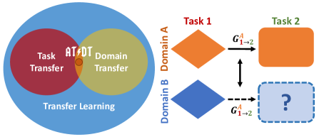
Figure 1: Our AT/DT framework transfers knowledge across tasks and domains. Given two tasks (1 and 2) and two domains (A and B), with supervision for both tasks in A but only for one task in B, we learn the dependency between tasks in A and exploit this knowledge in B to solve task 2 without the need of supervision.

A partial answer to this question has been provided by [44], which formalizes the relationships between tasks within a specific domain into a graph referred to as Taskonomy. This knowledge can be used to improve performance within a fully supervised learning scenario, though it is not clear how well may it generalize to new domains and to which extent may it be deployed in a partially supervised scenario (i.e., supervision on only some tasks/domains). Generalization to new domains is addressed in the domain adaptation literature [39], that, however, works under the assumption of solving a single task in isolation, therefore ignoring potential benefits from related tasks.

We fuse the two worlds by explicitly addressing a cross domain and cross task problem where on one domain (e.g., synthetic data) we have annotations for many tasks, while in the other (e.g., real data) annotations are available only for a specific task, though we wish to solve many.

Purposely, we propose a new ‘Across Tasks and Domains Transfer framework’ (shortened AT/DT ) which learns in a specific domain a function $G_{1\rightarrow 2}$ to transfer knowledge between a pair of tasks. After the training phase, we show that the same function can be applied in a new domain to solve the second task while relying on supervision only for the first. A schematic representation of AT/DT is pictured in Fig. 1.

We prove the effectiveness of AT/DT on a challenging autonomous driving scenario where we address the two related tasks of depth estimation and semantic segmentation [30]. Our framework allows the use of fully supervised synthetic datasets (i.e., Synthia [17], and Carla [7]) to drastically boost performance on partially supervised real data (i.e., Cityscapes [5] and Kitti [11, 28]). Finally, we will also show how AT/DT is robust to sub-optimal scenarios where we use only few annotated real samples or noisy supervision by proxy labels [23, 41, 35]. The novel contributions of this paper can be summarized as follows:

• According to the definition of task in [44], to the best of our knowledge we are the first to study a cross domain and cross task problem where supervision for all tasks is available in one domain whilst only for a subset of them in the other.

• We propose a general framework to address the aforementioned problem that learns to transfer knowledge across tasks and domains

• We show that it is possible to directly learn a mapping between features suitable for different tasks in a first domain and that this function generalizes to unseen data both in the source domain as well as in a second target domain.

2 Related Work

Transfer Learning: The existence of related representation within CNNs trained for different tasks has been highlighted since early works in the field [42]. These early findings have motivated the use of transfer learning strategy to bootstrap learning across related tasks. For example, object detection networks are typically initialized with Imagenet weights [32, 16, 25], although [15] has recently challenged this paradigm. Luo et al. [27] fuse transfer learning with domain adaptation to transfer representations across tasks and domains. However, their definition of tasks deals with different sets of classes in a classification problem, while we consider diverse visual tasks as set forth in [44]. Recently Zamir et. al. [44] have tried to formalize and deploy the idea of reusing information across training processes by proposing a computational approach to establish relationships among visual tasks represented in a taxonomy. Pal et. al. [29], propose to use similar knowledge alongside with meta-learning to learn how to perform a new task within a zero-shot scenario. Both [44] and [29] assume a shared domain across the addressed task, whilst we directly target a cross domain scenario. Moreover, [44] assumes full supervision to be available for all tasks while [29] zero supervision for the target task, Differently, our work leverages on full supervision for all tasks in one domain and only partial supervision in a different (target) domain.

Multi-task Learning: Multi-task learning tries to learn many tasks simultaneously to obtain more general models or multiple outputs in a single run [24, 6, 14]. Some recent works have addressed the autonomous driving scenario [3, 30] so to learn jointly related tasks like depth estimation and semantic segmentation in order to improve performance. Kendall et al. [4] additionally consider the instance segmentation task and show that it is possible to train a single network to solve the three tasks by fusing the different losses through uncertainty estimation. Our work, instead, directly targets a single task but tries to use the relationship between related tasks to alleviate the need for annotations.

Domain Adaptation: A recent survey of the domain adaptation literature can be found in [40]. The idea behind this field is to learn models that turn out robust when tested on data sampled from a domain different than the training one. Earliest approaches such as [12, 13] try to build intermediate representations across domains, while recent ones, specifically designed for deep learning, focus on adversarial training at either pixel or feature level. Pixel level methods [34, 47, 2, 31] seek to transform input images from one domain into the other one using recently proposed image-to-image translation GANs [48, 22]. Conversely, feature level methods [20, 26, 38, 37, 9, 45, 36] try to align the feature representation extracted from CNN across different datasets, usually, again, by using GANs. Finally, recent works [33, 19, 46] operate at both pixel and feature level and focus on a single specific task (usually semantic segmentation), while our framework leverages information from different tasks. As such, we argue that our new formulation can be seen as complementary to existing domain adaptation techniques.

3 Across Task and Domain Transfer Framework

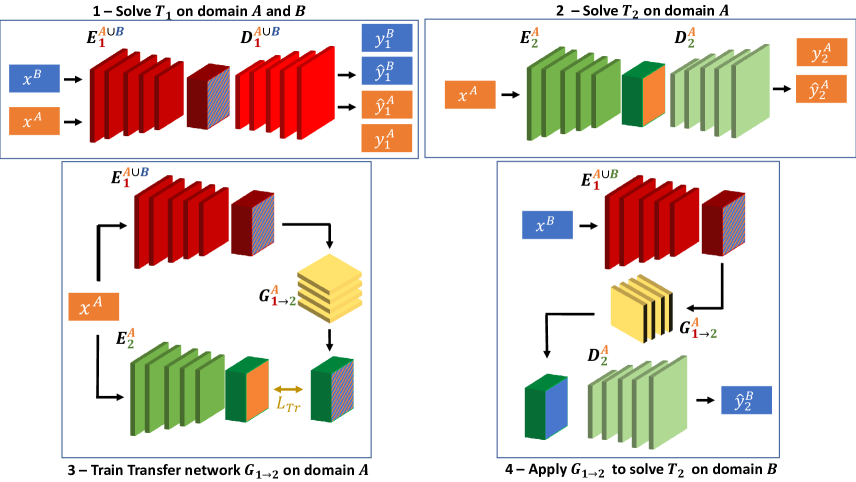
Figure 2: Overview of the AT/DT framework. (1) We train network $N_{1}^{A\cup{B}}$ to solve $\mathcal{T}_{1}$ (red) with supervision in domain $\mathcal{A}$ (orange) and $\mathcal{B}$ (blue) to obtain a shared feature representation across domains, highlighted by blue and orange strips. (2) We train a network $N_{2}^{A}$ to solve $\mathcal{T}_{2}$ (green) on $\mathcal{A}$ where labels are available. (3) We learn a network $G_{1\rightarrow 2}$ that transform features from $\mathcal{T}_{1}$ to $\mathcal{T}_{2}$ on samples from $\mathcal{A}$. (4) We apply the transfer network on $\mathcal{B}$ to solve $\mathcal{T}_{2}$ without the need for annotations.

We wish to start with a practical example of the problem we are trying to solve and how we address it. Let us consider a synthetic and a real domain where we aim to solve the semantic segmentation task. Annotations come for free in the synthetic domain while are rather expensive in the real one. Domain adaptation comes handy for this; however, we wish to go one step further. May we pick a closely related task (e.g., depth estimation) where annotations are available in both domains and use it to boost the performance of semantic segmentation on real data? To achieve this goal we train deep networks for depth and semantic segmentation on the synthetic domain and learn a mapping function to transform deep features suitable for depth estimation into deep features suitable for semantic segmentation. Then we apply the same mapping function on samples from the real domain to obtain a semantic segmentation model without the need of semantic labels in the real domain. In the remainder of this section, we formalize the AT/DT framework.

3.1 Common Notation

We denote with $\mathcal{T}_{j}$ a generic visual task defined as in [44]. Let us assume $\mathcal{X}^{k}$ to be the set of samples (i.e., images) belonging to domain k and $\mathcal{Y}_{j}^{k}$ to be the paired set of annotations for task $\mathcal{T}_{j}$. In our problem we assumes to have two domains, $\mathcal{A}$ and $\mathcal{B}$, and two tasks, $\mathcal{T}_{1}$ and $\mathcal{T}_{2}$. For the two tasks we have complete supervision in $\mathcal{A}$, i.e., ${\mathcal{Y}^{A}_{1}}$ and ${\mathcal{Y}^{A}_{2}}$, but labels only for $\mathcal{T}_{1}$ in $\mathcal{B}$, i.e. $\mathcal{Y}^{B}_{1}$. We assume each task $\mathcal{T}_{j}$ to be solvable by a deep neural network $N_{j}$, consisting in a feature encoder $E_{j}$ and a feature decoder $D_{j}$, such that $\hat{y}_{j}=N_{j}(x)=D_{j}(E_{j}(x))$. The network is trained on domain $k$ by minimizing a task-specific loss on annotated samples $(x^{k},y^{k}_{j})\sim(\mathcal{X}^{k},\mathcal{Y}_{j}^{k})$. The result of this training is a network trained to solve $\mathcal{T}_{j}$ using samples from $\mathcal{X}^{k}$ that we denote as $N_{j}^{k}$.

3.2 Overview

Our work builds on the intuition that if two tasks are related there should be a function $G_{1\rightarrow 2}:\mathcal{T}_{1}\rightarrow\mathcal{T}_{2}$ that transfer knowledge among them. But what does transferring knowledge actually means? We will show that this abstract concept can be implemented by transferring representations in deep feature spaces. We propose to first train two task specific networks, $N_{1}$ and $N_{2}$, then approximate function $G_{1\rightarrow 2}$ by a deep neural network that transforms features extracted by $N_{1}$ into corresponding features extracted by $N_{2}$ (i.e., $G_{1\rightarrow 2}:E_{1}(x)\rightarrow E_{2}(x)$). We train $G_{1\rightarrow 2}$ by minimizing a reconstruction loss on $\mathcal{A}$, where we have complete supervision for both tasks, and use it on $\mathcal{B}$ to solve $\mathcal{T}_{2}$ having supervision only for $\mathcal{T}_{1}$.

Our method can be summarized into the four steps pictured in Fig. 2 and detailed in the following sections:

1. Learn to solve task $\mathcal{T}_{1}$ on domains $\mathcal{A}$ and $\mathcal{B}$.

2. Learn to solve task $\mathcal{T}_{2}$ on domain $\mathcal{A}$.

3. Train $G_{1\rightarrow 2}$ on domain $\mathcal{A}$.

4. Apply $G_{1\rightarrow 2}$ to solve $\mathcal{T}_{2}$ on domain $\mathcal{B}$.

3.3 Solve $\mathcal{T}_{1}$ on $\mathcal{A}$ and $\mathcal{B}$

A network $N_{1}$ can be trained to solve task $\mathcal{T}_{1}$ on domain $\mathcal{X}^{k}$ by minimizing a task specific supervised loss

$$L_{\mathcal{T}_{1}}(\hat{y}_{1}^{k},y_{1}^{k});\;\hat{y}_{1}^{k}=N_{1}(x^{k}).$$ (1)

However, training one network for each domain would likely result in disjoint feature spaces; we, instead, wish to have similar representation to ease generalization of $G_{1\rightarrow 2}$ across domains. Therefore, we train a single network, $N_{1}^{A\cup{B}}$, on samples from both domains, i.e., $\mathcal{X}^{k}=\mathcal{X}^{A}\cup{\mathcal{X}^{B}}$. Having a common representation ease the learning of a task transfer mapping valid on both domains though training it only on $\mathcal{A}$. More details on the impact of having common or disjoint networks are reported in Sec. 6.2.

3.4 Solve $\mathcal{T}_{2}$ on $\mathcal{A}$

Now we wish to train a network to solve $\mathcal{T}_{2}$, however, for this task we can only rely on annotated samples from $\mathcal{A}$. The best we can do is to train a $N_{2}^{A}$ minimizing a supervised loss

$$L_{\mathcal{T}_{2}}(\hat{y}_{2}^{A},y_{2}^{A});\;\hat{y}_{2}^{A}=N_{2}(x^{A}).$$ (2)

3.5 Train $G_{1\rightarrow 2}$ on $\mathcal{A}$

We are now ready to train a task transfer network $G_{1\rightarrow 2}$ that should learn to remap deep features suitable for $\mathcal{T}_{1}$ into good representations suitable for $\mathcal{T}_{2}$. Given $N_{1}^{A\cup{B}}$ and $N_{2}^{A}$ we generate a training set with pairs of features $(E_{1}^{A\cup{B}}(x^{A}),E_{2}(x^{A}))$ obtained feeding the same input $x^{A}$ to $N_{1}^{A\cup{B}}$ and $N_{2}^{A}$. We use only samples from $\mathcal{A}$ for the training set as it is the only domain where we are reasonably sure that the two networks perform well. We optimize the parameters of $G_{1\rightarrow 2}$ by minimizing the reconstruction error between transformed and target features

$$L_{Tr}=||G_{1\rightarrow 2}(E_{1}^{A\cup{B}}(x^{A}))-E_{2}^{A}(x^{A})))||_{2},$$ (3)

At the end of the training $G_{1\rightarrow 2}$ should have learned how to remap deep features from one space into the other.

Among all the possible splits $(E,D)$ obtained cutting $N$ at different layers, we select as input for $G_{1\rightarrow 2}$ the deepest features, i.e., those at the lowest spatial resolution. We make this choice because deeper features tend to be less connected to a specific domain and more correlated to higher level concepts. Therefore, by learning a mapping at this level we hope to suffer less from domain shift when applying $G_{1\rightarrow 2}$ on samples from $\mathcal{B}$. A more in depth discussion on the choice of $E$ is reported in Sec. 6.1. Additional considerations on the key role of $G_{1\rightarrow 2}$ in our framework can be found in the supplementary material.

3.6 Apply $G_{1\rightarrow 2}$ to solve $\mathcal{T}_{2}$ on $\mathcal{B}$

Now we aim to solve $\mathcal{T}_{2}$ on $\mathcal{B}$. We can use the supervision provided for $\mathcal{T}_{1}$ on $\mathcal{B}$ to extract good image features (i.e., $E^{A\cup{B}}_{1}(x_{B})$ ). Then use $G_{1\rightarrow 2}$ to transform these features into good features for $\mathcal{T}_{2}$, and finally decode them through a suitable decoder $D^{A}_{2}$. The whole system at inference time corresponds to:

$$\hat{y}^{B}_{2}=D^{A}_{2}(G^{A}_{1\rightarrow 2}(E^{A\cup{B}}_{1}(x_{B})))$$ (4)

Thus, thanks to our novel formulation, we can learn through supervision the dependencies between two tasks in a source domain and leverage on them to perform one of the two tasks in a different target domain where annotations are not available.

4 Experimental Settings

We describe here the experimental choices made when testing AT/DT, with additional details provided in the supplementary material due space constraints.

Tasks. To validate the effectiveness of AT/DT, we select as $\mathcal{T}_{1}$ and $\mathcal{T}_{2}$ semantic segmentation and monocular depth estimation. In the supplementary material, we report some promising results also for other tasks. We minimize a cross entropy loss to train a network for semantic segmentation while we use a $L_{1}$ regression loss to train a network for monocular depth estimation. We choose these two tasks since they are closely related, as highlighted in recent works [30, 3, 4], and of clear interest in many practical settings such as, e.g., autonomous driving. Moreover, as both tasks require a structured output, they can be addressed by a similar network architecture with the only difference being the number of filters in the final layer: as many as the number of classes for semantic segmentation and just one for depth estimation.

Datasets. We consider four different datasets, two synthetic ones, and two real ones. We pick synthetic datasets as $\mathcal{A}$ to learn the mapping across tasks thanks to availability of free annotations. We use real dataset as $\mathcal{B}$ to benchmark the performance of AT/DT in challenging realistic conditions. As synthetic datasets we have used the six video sequences of the Synthia-SF dataset [17] (shortened as Synthia) and rendered several other sequences with the Carla simulator [7]. For both datasets, we have split the data into a train, validation, and test set by subdividing them at the sequence level (i.e., we have used different sequences for train, validation, and test). As for the real datasets, we have used images from the Kitti [11, 28, 10] and Cityscapes [5] benchmarks. Concerning Kitti, we have used the 200 images from the Kitti 2012 training set [11] to benchmark depth estimation and 200 images from the Kitti 2015 training set with semantic annotations recently released in [1]. As for Cityscapes, we have used the validation split to benchmark semantic segmentation and all the images in the training split. When training depth estimation networks on Cityscapes, following a procedure similar to [35] we generate proxy labels by filtering SGM [18] disparities through confidence measures (left-right check).

	$\mathcal{A}$	$\mathcal{B}$	Method	Road	Sidewalk	Walls	Fence	Person	Poles	Vegetation	Vehicles	Tr. Signs	Building	Sky	mIoU	Acc
(a)	Synthia	Carla	Baseline	63.94	54.87	15.21	0.03	13.55	12.78	52.73	27.34	4.88	50.24	79.73	34.12	73.36
	Synthia	Carla	AT/DT	73.57	62.58	26.85	0.00	17.79	37.30	35.27	52.94	17.76	62.99	87.50	43.14	80.00
(b)	Synthia	Cityscapes	Baseline	6.91	0.68	0.00	0.00	2.47	9.14	3.19	8.90	0.81	25.93	26.86	7.72	28.49
	Synthia	Cityscapes	AT/DT	85.77	29.40	1.23	0.00	3.72	14.55	1.87	8.85	0.38	42.79	67.06	23.24	64.03
(c)	Carla	Cityscapes	Baseline	71.87	36.53	3.99	6.66	24.33	22.20	66.06	48.12	7.60	60.22	69.05	37.88	74.61
	Carla	Cityscapes	AT/DT	76.44	32.24	4.75	5.58	24.49	24.95	68.98	40.49	10.78	69.38	78.19	39.66	76.37
	-	Cityscapes	Oracle	95.65	77.72	33.02	37.63	65.45	42.087	89.36	89.99	41.36	86.81	89.22	68.02	93.56

Table 1: Experimental results of $Dep.\rightarrow Sem.$ scenario. Best results highlighted in bold.

Network Architecture. Each task network is implemented as a dilated ResNet50 [43] that compresses an image to $1/16$ of the input resolution to extract features. Then we use several bilinear up-sample and convolutional layers to regain resolution and get to the final prediction layer. All the layers of the network feature batch normalization. We implement the task transfer network ($G_{1\rightarrow 2}$) as a simple stack of convolutional and deconvolutional layers that reduce the input to $1/4$ of the input resolution before getting back to the original scale.

Evaluation Protocol. For each test we select two domains (i.e., two datasets, referred to as $\mathcal{A}$ and $\mathcal{B}$) and one direction of task transfer, e.g., from $\mathcal{T}_{1}$ to $\mathcal{T}_{2}$. We will use $Sem.\rightarrow Dep.$ when mapping features from semantics to depth and $Dep.\rightarrow Sem.$ when switching the two tasks. For each configuration of datasets and tasks we use AT/DT to train a cross-task network ($G_{1\rightarrow 2}$) following the protocol described in Sec. 3.2, then measure its performance for $\mathcal{T}_{2}$ on $\mathcal{B}$. We compare our method against a Baseline obtained training a network with supervision for $\mathcal{T}_{2}$ in $\mathcal{A}$ (i.e., $N_{2}^{A}$) and testing it on $\mathcal{B}$. Moreover, we report as a reference the performance attainable by a Oracle (i.e., a network trained with supervision on $\mathcal{B}$).

Metrics. Our semantic segmentation networks predict eleven different classes corresponding to those available in the Carla simulator plus one additional class for ‘Sky’. To measure performance, we report two different global metrics: pixel accuracy, shortened Acc. (i.e., the percentage of pixels with a correct label) and Mean Intersection Over Union, shortened mIoU (computed as detailed in [5]). To provide more insights on per-class gains we also report the IoU (intersection-over-union) score computed independently for each class.

When testing the depth estimation task we use the standard metrics described in [8]: Absolute Relative Error (Abs Rel), Square Relative Error (Sq Rel), Root Mean Square Error (RMSE), logarithmic RMSE and three $\delta$ accuracy scores ($\delta_{\alpha}$ being the percentage of predictions whose maximum between ratio and inverse ratio with respect to the ground truth is lower than $1.25^{\alpha}$).

5 Experimental Results

				blue!25Lower is better				LightCyanHigher is better
	$\mathcal{A}$	$\mathcal{B}$	Method	blue!25Abs Rel	blue!25Sq Rel	blue!25RMSE	blue!25RMSE log	LightCyan$\delta_{1}$	LightCyan$\delta_{2}$	LightCyan$\delta_{3}$
(a)	Synthia	Carla	Baseline	0.632	8.922	13.464	0.664	0.323	0.578	0.733
	Synthia	Carla	AT/DT	0.316	5.485	11.712	0.458	0.553	0.785	0.880
(b)	Carla	Cityscapes	Baseline	0.667	13.500	16.875	0.593	0.276	0.566	0.770
	Carla	Cityscapes	AT/DT	0.394	5.837	13.915	0.435	0.337	0.749	0.899
	Cityscapes	Cityscapes	Oracle	0.176	3.116	9.645	0.256	0.781	0.921	0.969
(c)	Carla	Kitti	Baseline	0.500	10.602	10.772	0.487	0.384	0.723	0.853
	Carla	Kitti	AT/DT	0.439	8.263	9.148	0.421	0.483	0.788	0.891
	-	Kitti	Oracle	0.265	2.256	5.696	0.319	0.672	0.859	0.939

Table 2: Experimental results of $Sem.\rightarrow Dep.$ scenario. Best results highlighted in bold.

We subdivide the experimental results in three main sections: in Sec. 5.1 and Sec. 5.2 we transfer information between semantic segmentation and depth estimation, while in Sec. 5.3 we show preliminary results on the integration of AT/DT with domain adaptation techniques.

5.1 Depth to Semantics

Following the protocol detailed in Sec. 4, we first test AT/DT when transferring knowledge from the monocular depth estimation task to the semantic segmentation task, and report the results in Tab. 1. In this setup, we have supervision for both tasks in $\mathcal{A}$ while only for depth estimation in $\mathcal{B}$. Therefore, for each configuration, we report the results obtained performing semantic segmentation on $\mathcal{B}$ without any domain-specific supervision.

We begin our investigation by studying the task transfer in a purely synthetic environment, where we can have perfect annotations for all tasks and domains, i.e., we use Synthia and Carla as $\mathcal{A}$ and $\mathcal{B}$, respectively. The results obtained by AT/DT and a transfer learning baseline are reported in Tab. 1-(a). Comparing the two rows we can clearly see that our method boost performance by +9.02% and +6,64%, for mIoU and Acc, respectively, thanks to the additional knowledge transferred from the depth estimation task.

The same performance boost holds when considering a far more challenging domain transfer between synthetic and real data, i.e., Tab. 1-(b) (Synthia $\rightarrow$ Cityscapes) and Tab. 1-(c) (Carla $\rightarrow$ Cityscapes). In both scenarios, our AT/DT improves the two averaged metrics (mIoU and Acc.) and most of the per class scores, with gain as large as +78,86% for the Road class in (b). Overall AT/DT consistently improves predictions for the more interesting classes in autonomous driving scenarios, e.g., Road, Person…. The main difficulties for AT/DT seems to deal with transferring knowledge for classes where depth estimation is particularly hard (e.g., Vegetation, where synthetic data have far from optimal annotations, or thin structures like Poles and Fences). Indeed our model in Tab. 1-(c) is still far from the performance obtainable by the same Oracle network trained with supervision on $\mathcal{B}$ for $\mathcal{T}_{2}$. However we wish to point out that in this scenario we do not use any annotation at all on the real Cityscapes data, since we automatically generate noisy proxy labels for depth from synchronized stereo frames following [35].

The top row of Fig. 3 show qualitative results on Cityscapes where AT/DT produces clearly better semantic maps than the baseline network.

5.2 Semantics to Depth

Following the protocol detailed in Sec. 4, we test AT/DT when transferring features from semantic segmentation to monocular depth estimation. In this setup, we have complete supervision for both tasks in $\mathcal{A}$ and only for semantic segmentation in $\mathcal{B}$. For each configuration we report in Tab. 2 the results obtained performing monocular depth estimation on $\mathcal{B}$ without any domain-specific supervision.

The first pair of rows (i.e., Tab. 2-(a)) reports results when transferring knowledge across two synthetic domains. The use of knowledge coming from semantic features helps AT/DT to predict better depths resulting in consistent improvements in all the seven metrics with respect to the baseline. The same gains hold for tests concerning real datasets (i.e., Tab. 2-(b) with Cityscapes and Tab. 2-(c) with Kitti), where the deployment of AT/DT always results in a clear advantage against the baseline. We wish to point out how on Tab. 2-(c) we report a result where AT/DT use very few annotated samples from $\mathcal{B}$ (i.e., only the 200 images annotated with semantic labels released by [1]). Comparing Tab. 2-(c) to Tab. 2-(b) we can see how the low data regime of Kitti results in slightly smaller gains, as also testified by the difference among oracle performances in the two datasets. Nevertheless AT/DT consistently yields improvements with respect to the baseline for all the seven metrics. We believe that these results provide some assurances on the effectiveness of AT/DT with respect to the amount of available data per task. Finally, the bottom row of Fig. 3 shows qualitative results on monocular depth estimation on Cityscapes: we can clearly observe how AT/DT provides significant improvements over the baseline, especially on far objects.

Input	Baseline	AT/DT	GT

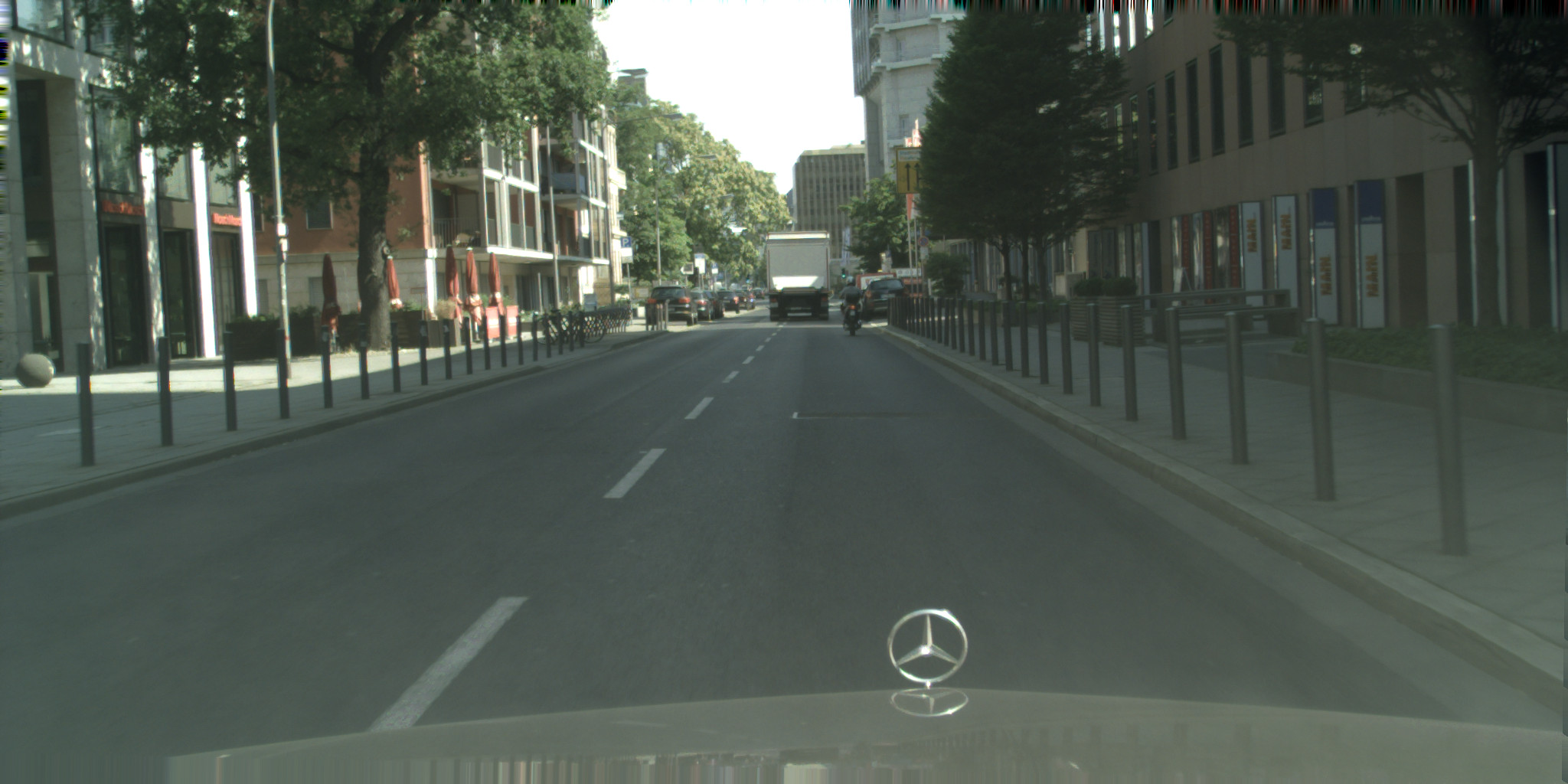
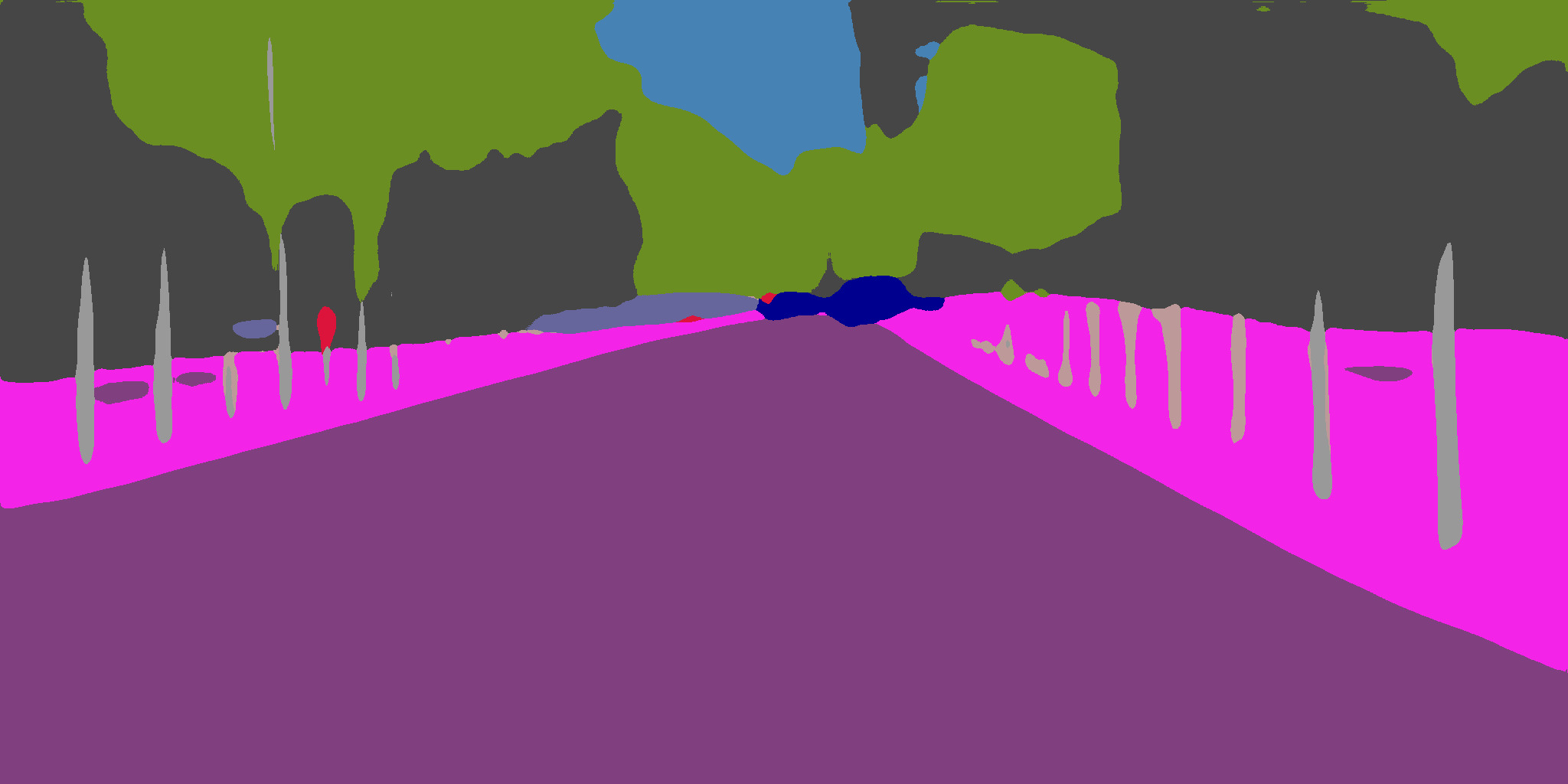
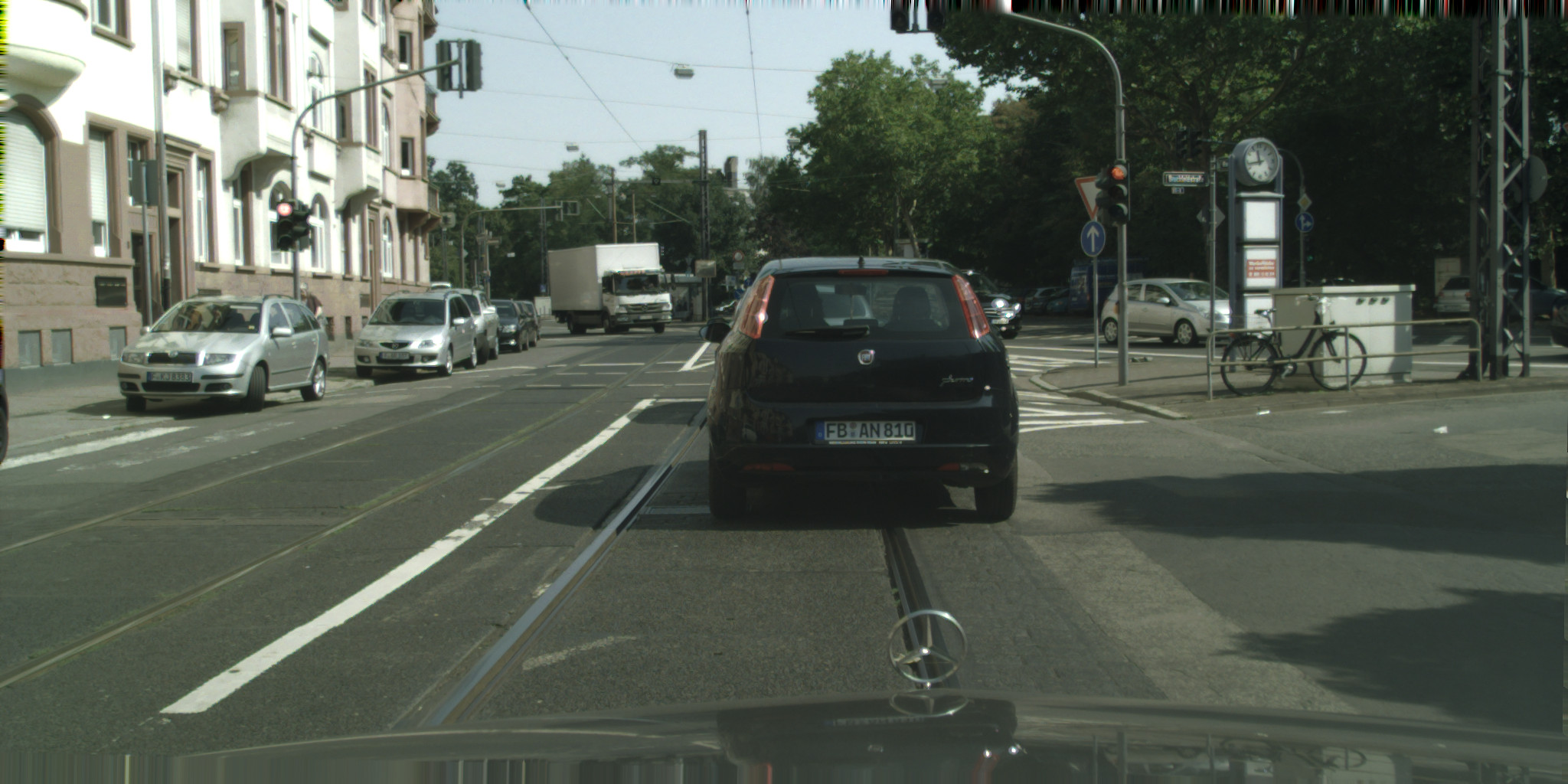
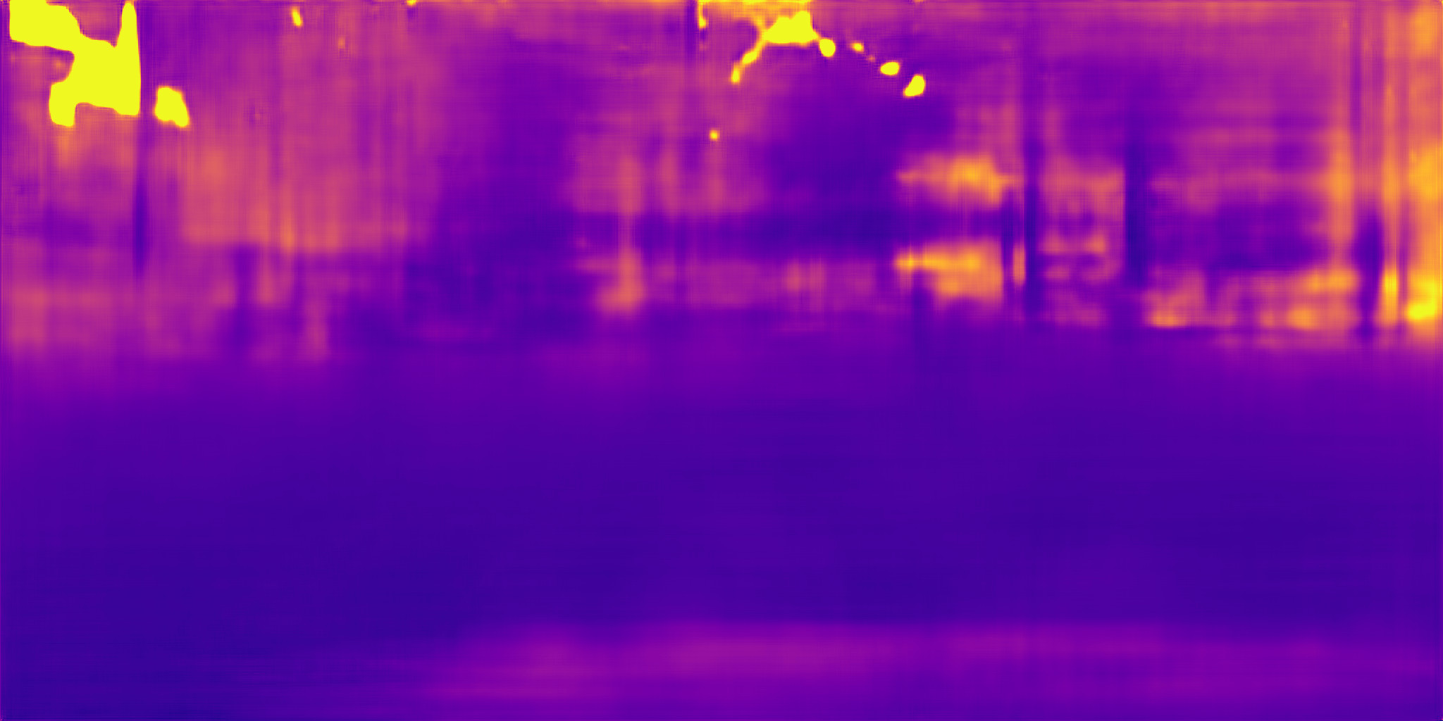
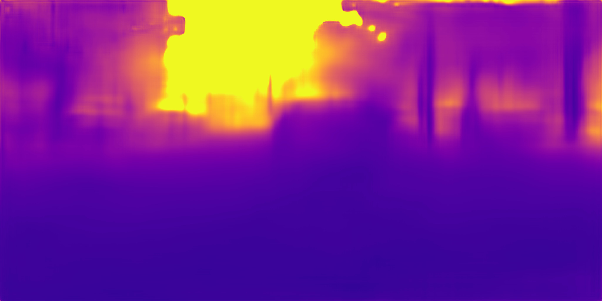
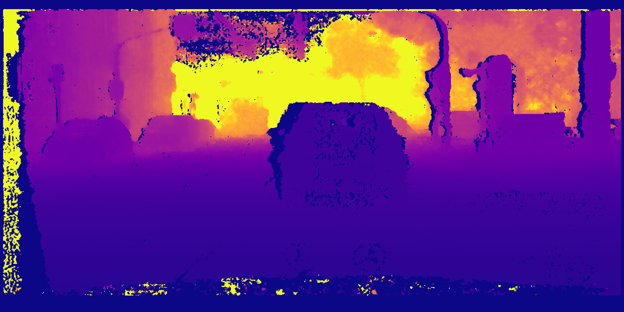
Figure 3: Qualitative results for $\mathcal{A}$: Carla to $\mathcal{B}$: Cityscapes. First row shows $Dep.\rightarrow Sem.$ scenario while second row shows $Sem.\rightarrow Dep.$ setting. From left to right RGB input, baseline predictions, AT/DT predictions, ground-truth images.

5.3 Integration with Domain Adaptation

	Method	Road	Sidewalk	Walls	Fence	Person	Poles	Vegetation	Vehicles	Tr. Signs	Building	Sky	mIoU	Acc
(a)	Baseline	71.87	36.53	3.99	6.66	24.33	22.20	66.06	48.12	7.60	60.22	69.05	37.88	74.61
(b)	AT/DT	76.44	32.24	4.75	5.58	24.49	24.95	68.98	40.49	10.78	69.38	78.19	39.66	76.37
(c)	CycleGAN	81.58	39.15	6.08	5.31	30.22	21.73	77.71	50.00	8.33	68.35	77.22	42.33	80.93
(d)	AT/DT + CycleGAN	85.19	41.37	5.44	3.02	29.90	24.07	71.93	58.09	7.53	70.90	77.78	43.20	81.92

Table 3: Experimental results of integration with domain adaptation techniques. We show results of $\mathcal{A}$: Carla to $\mathcal{B}$: Cityscapes and $Dep.\rightarrow Sem.$ scenario. Best results highlighted in bold.

		blue!25Lower is better				LightCyanHigher is better
	Method	blue!25Abs Rel	blue!25Sq Rel	blue!25RMSE	blue!25RMSE log	LightCyan$\delta_{1}$	LightCyan$\delta_{2}$	LightCyan$\delta_{3}$
(a)	Baseline	0.667	13.499	16.875	0.593	0.276	0.566	0.770
(b)	AT/DT	0.394	5.837	13.915	0.435	0.337	0.749	0.899
(c)	CycleGAN	0.943	27.026	21.666	0.695	0.218	0.478	0.690
(d)	AT/DT+CycleGAN	0.563	10.789	15.636	0.489	0.247	0.668	0.861

Table 4: Experimental results of comparison and integration with domain adaptation techniques. We show results of $\mathcal{A}$: Carla to $\mathcal{B}$: Cityscapes and $Sem.\rightarrow Dep.$ scenario. Best results highlighted in bold.

All the results of Sec. 5.1 and Sec. 5.2 are obtained learning a mapping function across tasks in a domain and deploying it in another one. Therefore, both the transfer network $G_{1\rightarrow 2}$ and the baseline we consider, can indeed suffer from domain shift issues. Fortunately, the domain adaptation literature provides several different strategies to overcome domain shifts that are complementary to our AT/DT. We provide here some preliminary results on how the two approaches may be combined together. We consider a pixel-level domain adaptation technique, i.e., CycleGan [48], that transforms images from $\mathcal{B}$ to render them more similar to those from $\mathcal{A}$. In Tab. 3, we report results obtained for a $Dep.\rightarrow Sem.$ scenario using Carla as $\mathcal{A}$ and Cityscapes as $\mathcal{B}$. The pixel level domain alignment of CycleGAN (row (c)) proves particularly effective in this scenario, yielding a huge boost when compared to the baseline (row (a)), even greater then the gain granted by AT/DT (row (b)). However, we can see how the best average results (i.e., mIoU and Acc.) can be obtained combining our cross task framework (AT/DT) with the pixel level domain adaptation provided by CycleGAN (row (d)). Considering the scores on single classes, instead, there is no clear winner among the four considered methods, with different algorithms providing higher accuracy for different classes. In Tab. 4 we report results obtained on a $Sem.\rightarrow Dep.$ scenario using the same pair of domains and the same four methods. Surprisingly, when targeting depth estimation CycleGAN (row (c)) is not as effective as before and actually worsen significantly the performance of the baseline (row (a)). Our AT/DT is instead more robust to the task being addressed and in this scenario can improve the baseline when combined with CycleGAN (row (d)) and obtain the best overall results when applied alone (row (a)).

6 Additional Experiments

We report additional tests to shine light on some of the design choices made when developing AT/DT. Moreover, in the supplementary material we propose an experimental study focused on highlighting the importance of $G_{1\rightarrow 2}$, in particular comparing our proposal to an end-to-end multi-task network featuring a shared encoder and two task dependent decoders.

6.1 Study on the Transfer Level

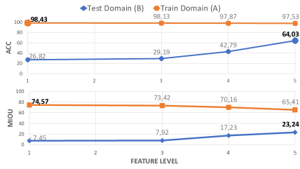
Figure 4: Study on feature level for task transfer from Synthia to Cityscapes and $Dep.\rightarrow Sem.$ scenario. Deeper levels correspond to higher generalization performances.

For all the previous tests we split $N$ between $E$ and $D$ at the layer corresponding to the lowest spatial resolution. We pick this split based on the intuition that deeper layers yield more abstract representations, thus less correlated to specific domain information, while lower level features are more domain dependent. Therefore, learning $G_{1\rightarrow 2}$ between shallower layers should lead to less generalization ability across domains. To validate this intuition, we run experiments aimed at measuring performance for the $Dep.\rightarrow Sem.$ scenario (Synthia $\rightarrow$ Cityscapes) when varying the network layer at which we split $N$ into $E$ and $D$. We consider four different feature levels corresponding to residual blocks at increasing depth in ResNet50. For each of them we train a transfer network on domain $\mathcal{A}$ and then measure mIoU and Acc. testing on unseen images from $\mathcal{A}$ (i.e. $D_{2}^{A}(G^{A}_{1\rightarrow 2}(E_{1}^{AuB}(x_{A})))$) and $\mathcal{B}$ (i.e. $D_{2}^{A}(G^{A}_{1\rightarrow 2}(E_{1}^{AuB}(x_{B})))$). The results are plotted in Fig. 4.

Considering Acc. (top plot) we can see how in-domain performance are almost equivalent at the different feature levels (orange line), while cross-domain performance increase when considering deeper feature levels (blue line). This pattern is even more pronounced when considering mIoU (bottom plot), where in-domain performance actually decreases alongside with deeper feature, whilst cross-domain performance increases. These results validate our intuition that deeper features are less domain specific and may lead to better generalization to unseen domains.

6.2 Shared vs Non-Shared $N_{1}$

Shared	Domain	mIoU	Acc.
✗	$\mathcal{A}$	61.73	97.02
✓	$\mathcal{A}$	65.41	97.53
✗	$\mathcal{B}$	6.42	29.36
✓	$\mathcal{B}$	23.24 (+16.82)	64.03 (+34.67)

Table 5: Study on Shared vs Non-Shared $N_{1}^{A\cup{B}}$. We show a $\mathcal{A}$: Synthia to $\mathcal{B}$: Carla and $Dep.\rightarrow Sem.$ scenario. Performance improvement highlighted in bold.

Throughout this work we have always trained a single network for $\mathcal{T}_{1}$ with samples from $\mathcal{A}$ and $\mathcal{B}$. The rationale behind this choice is to have a single feature extractor for both domains such that $G_{1\rightarrow 2}$ trained only on samples from $\mathcal{A}$ would be able to generalize well to samples from $\mathcal{B}$ as they are sampled from a similar distribution.

Here we experimentally validate this intuition by comparing a shared $N_{1}^{A\cup{B}}$ against the use of two separate networks, one trained on samples from $\mathcal{A}$ ($N_{1}^{A}$) and the other with samples from $\mathcal{B}$ ($N_{1}^{B}$). We consider a $Dep.\rightarrow Sem.$ scenario where we use Synthia as domain $\mathcal{A}$ and Cityscapes as $\mathcal{B}$. In Tab. 5 we report the mIoU and Acc. achieved on unseen samples from the two domains. On the training domain $\mathcal{A}$ both methods are able to obtain good results, slightly better for the shared network, probably thanks to the higher variety of data used for training. However, when moving to the completely different domain $\mathcal{B}$, it is clear that maintaining the same feature extractor is of crucial importance to be able to use the same $G_{1\rightarrow 2}$. This test suggests the interesting findings that feature extracted by the exact same network architecture trained for the exact same tasks in two different domains are quite different. Therefore to correctly apply $G_{1\rightarrow 2}$ we need to take into account these difficulties.

6.3 Batch Normalization

Batchnorm	Domain	mIoU	Acc.
✗	$\mathcal{A}$	72.48	98.09
✓	$\mathcal{A}$	65.41	97.53
✗	$\mathcal{B}$	22.75	58.29
✓	$\mathcal{B}$	23.24 (+0.49)	64.03 (+5.74)

Table 6: Ablation Study on Batch Normalization. We show a $\mathcal{A}$: Synthia to $\mathcal{B}$: Cityscapes and $Dep.\rightarrow Sem.$ scenario. Performance improvement highlighted in bold.

We investigate the impact on performance of using task networks with or without batch normalization layers [21]. Our intuition is that the introduction of batch normalization yields more similar features across domains and smaller numerical values, making the training of $G_{1\rightarrow 2}$ easier and numerically more stable. In Tab. 6 we report results for the $Dep.\rightarrow Sem.$ scenario when employing Synthia as $\mathcal{A}$ and Cityscapes as $\mathcal{B}$. As expected, batch normalization yields representations more similar between domains, thus leading to better generalization performances on $\mathcal{B}$. Counter-intuitively, we also notice that results on $\mathcal{A}$ are worse with batch normalization, perhaps due to mapping features from $\mathcal{T}_{1}$ to $\mathcal{T}_{2}$ being harder when these lay within a more constrained space.

7 Conclusion and Future Works

We have shown that it is possible to learn a mapping function to transform deep representations suitable for specific tasks into others amenable to different ones. Our methods allows for leveraging on easy to annotate domains to solve tasks in scenarios where annotations would be costly. We have shown promising results obtained by applying our framework to two tasks (semantic segmentation and monocular depth estimation) and four different domains (two synthetic domains and two real domains). In future work, we plan to investigate on the effectiveness and robustness of our framework when addressing other tasks. In this respect, Taskonomy [44] may guide us in identifying tightly related visual tasks likely to enable effective transfer of learned representations. We have also shown preliminary results concerning how our framework may be fused with standard domain adaptation strategies in order to further ameliorate performance. We believe that finding the best strategy to fuse the two worlds is a novel and exciting research avenue set forth by our paper.

See supplementary See supplementary See supplementary See supplementary See supplementary

References

- [1] Hassan Alhaija, Siva Mustikovela, Lars Mescheder, Andreas Geiger, and Carsten Rother. Augmented reality meets computer vision: Efficient data generation for urban driving scenes. International Journal of Computer Vision (IJCV), 2018.
- [2] Konstantinos Bousmalis, Nathan Silberman, David Dohan, Dumitru Erhan, and Dilip Krishnan. Unsupervised pixel-level domain adaptation with generative adversarial networks. 2017 IEEE Conference on Computer Vision and Pattern Recognition (CVPR), Jul 2017.
- [3] Sumanth Chennupati, Ganesh Sistu, Senthil Yogamani, and Samir Rawashdeh. Auxnet: Auxiliary tasks enhanced semantic segmentation for automated driving, 2019.
- [4] Roberto Cipolla, Yarin Gal, and Alex Kendall. Multi-task learning using uncertainty to weigh losses for scene geometry and semantics. 2018 IEEE/CVF Conference on Computer Vision and Pattern Recognition, Jun 2018.
- [5] Marius Cordts, Mohamed Omran, Sebastian Ramos, Timo Rehfeld, Markus Enzweiler, Rodrigo Benenson, Uwe Franke, Stefan Roth, and Bernt Schiele. The cityscapes dataset for semantic urban scene understanding. In The IEEE Conference on Computer Vision and Pattern Recognition (CVPR), June 2016.
- [6] Carl Doersch and Andrew Zisserman. Multi-task self-supervised visual learning. 2017 IEEE International Conference on Computer Vision (ICCV), Oct 2017.
- [7] Alexey Dosovitskiy, German Ros, Felipe Codevilla, Antonio Lopez, and Vladlen Koltun. CARLA: An open urban driving simulator. In Proceedings of the 1st Annual Conference on Robot Learning, pages 1–16, 2017.
- [8] David Eigen, Christian Puhrsch, and Rob Fergus. Depth map prediction from a single image using a multi-scale deep network. In Advances in neural information processing systems, pages 2366–2374, 2014.
- [9] Yaroslav Ganin and Victor Lempitsky. Unsupervised domain adaptation by backpropagation. In International Conference on Machine Learning, pages 1180–1189, 2015.
- [10] Andreas Geiger, Philip Lenz, Christoph Stiller, and Raquel Urtasun. Vision meets robotics: The kitti dataset. International Journal of Robotics Research (IJRR), 2013.
- [11] Andreas Geiger, Philip Lenz, and Raquel Urtasun. Are we ready for autonomous driving? the kitti vision benchmark suite. In Computer Vision and Pattern Recognition (CVPR), 2012 IEEE Conference on, pages 3354–3361. IEEE, 2012.
- [12] Boqing Gong, Yuan Shi, Fei Sha, and Kristen Grauman. Geodesic flow kernel for unsupervised domain adaptation. In Computer Vision and Pattern Recognition (CVPR), 2012 IEEE Conference on, pages 2066–2073. IEEE, 2012.
- [13] Raghuraman Gopalan, Ruonan Li, and Rama Chellappa. Domain adaptation for object recognition: An unsupervised approach. In Computer Vision (ICCV), 2011 IEEE International Conference on, pages 999–1006. IEEE, 2011.
- [14] Michelle Guo, Albert Haque, De-An Huang, Serena Yeung, and Li Fei-Fei. Dynamic task prioritization for multitask learning. In The European Conference on Computer Vision (ECCV), September 2018.
- [15] Kaiming He, Ross Girshick, and Piotr Dollár. Rethinking imagenet pre-training, 2018.
- [16] Kaiming He, Georgia Gkioxari, Piotr Dollar, and Ross Girshick. Mask r-cnn. 2017 IEEE International Conference on Computer Vision (ICCV), Oct 2017.
- [17] Daniel Hernandez-Juarez, Lukas Schneider, Antonio Espinosa, David Vazquez, Antonio M. Lopez, Uwe Franke, Marc Pollefeys, and Juan Carlos Moure. Slanted stixels: Representing san francisco’s steepest streets. In British Machine Vision Conference (BMVC), 2017, 2017.
- [18] Heiko Hirschmuller. Accurate and efficient stereo processing by semi-global matching and mutual information. In Computer Vision and Pattern Recognition, 2005. CVPR 2005. IEEE Computer Society Conference on, volume 2, pages 807–814. IEEE, 2005.
- [19] Judy Hoffman, Eric Tzeng, Taesung Park, Jun-Yan Zhu, Phillip Isola, Kate Saenko, Alexei A. Efros, and Trevor Darrell. Cycada: Cycle-consistent adversarial domain adaptation, 2017.
- [20] Judy Hoffman, Dequan Wang, Fisher Yu, and Trevor Darrell. Fcns in the wild: Pixel-level adversarial and constraint-based adaptation. arXiv preprint arXiv:1612.02649, 2016.
- [21] Sergey Ioffe and Christian Szegedy. Batch normalization: Accelerating deep network training by reducing internal covariate shift. In Proceedings of the 32Nd International Conference on International Conference on Machine Learning - Volume 37, ICML’15, pages 448–456. JMLR.org, 2015.
- [22] Phillip Isola, Jun-Yan Zhu, Tinghui Zhou, and Alexei A. Efros. Image-to-image translation with conditional adversarial networks. In The IEEE Conference on Computer Vision and Pattern Recognition (CVPR), July 2017.
- [23] Maria Klodt and Andrea Vedaldi. Supervising the new with the old: learning sfm from sfm. In Proceedings of the European Conference on Computer Vision (ECCV), pages 698–713, 2018.
- [24] Iasonas Kokkinos. Ubernet: Training a universal convolutional neural network for low-, mid-, and high-level vision using diverse datasets and limited memory. 2017 IEEE Conference on Computer Vision and Pattern Recognition (CVPR), Jul 2017.
- [25] Wei Liu, Dragomir Anguelov, Dumitru Erhan, Christian Szegedy, Scott Reed, Cheng-Yang Fu, and Alexander C Berg. Ssd: Single shot multibox detector. In European conference on computer vision, pages 21–37. Springer, 2016.
- [26] Mingsheng Long, Yue Cao, Jianmin Wang, and Michael Jordan. Learning transferable features with deep adaptation networks. In Proceedings of the 32nd International Conference on Machine Learning, volume 37 of Proceedings of Machine Learning Research, pages 97–105. PMLR, 2015.
- [27] Zelun Luo, Yuliang Zou, Judy Hoffman, and Li F Fei-Fei. Label efficient learning of transferable representations acrosss domains and tasks. In Advances in Neural Information Processing Systems, pages 165–177, 2017.
- [28] Moritz Menze and Andreas Geiger. Object scene flow for autonomous vehicles. In Conference on Computer Vision and Pattern Recognition (CVPR), 2015.
- [29] Arghya Pal and Vineeth N Balasubramanian. Zero-shot task transfer, 2019.
- [30] Pierluigi Zama Ramirez, Matteo Poggi, Fabio Tosi, Stefano Mattoccia, and Luigi Di Stefano. Geometry meets semantics for semi-supervised monocular depth estimation. arXiv preprint arXiv:1810.04093, 2018.
- [31] Pierluigi Zama Ramirez, Alessio Tonioni, and Luigi Di Stefano. Exploiting semantics in adversarial training for image-level domain adaptation, 2018.
- [32] Shaoqing Ren, Kaiming He, Ross Girshick, and Jian Sun. Faster r-cnn: Towards real-time object detection with region proposal networks. IEEE Transactions on Pattern Analysis and Machine Intelligence, 39(6):1137–1149, Jun 2017.
- [33] Swami Sankaranarayanan, Yogesh Balaji, Arpit Jain, Ser Nam Lim, and Rama Chellappa. Learning from synthetic data: Addressing domain shift for semantic segmentation. 2018 IEEE/CVF Conference on Computer Vision and Pattern Recognition, Jun 2018.
- [34] Ashish Shrivastava, Tomas Pfister, Oncel Tuzel, Josh Susskind, Wenda Wang, and Russ Webb. Learning from simulated and unsupervised images through adversarial training. In The IEEE Conference on Computer Vision and Pattern Recognition (CVPR), 2017.
- [35] Alessio Tonioni, Matteo Poggi, Stefano Mattoccia, and Luigi Di Stefano. Unsupervised adaptation for deep stereo. In Proceedings of the IEEE International Conference on Computer Vision, pages 1605–1613, 2017.
- [36] Yi-Hsuan Tsai, Wei-Chih Hung, Samuel Schulter, Kihyuk Sohn, Ming-Hsuan Yang, and Manmohan Chandraker. Learning to adapt structured output space for semantic segmentation. 2018 IEEE/CVF Conference on Computer Vision and Pattern Recognition, Jun 2018.
- [37] Eric Tzeng, Judy Hoffman, Trevor Darrell, and Kate Saenko. Simultaneous deep transfer across domains and tasks. In Proceedings of the IEEE International Conference on Computer Vision, pages 4068–4076, 2015.
- [38] Eric Tzeng, Judy Hoffman, Kate Saenko, and Trevor Darrell. Adversarial discriminative domain adaptation. In Computer Vision and Pattern Recognition (CVPR), 2017.
- [39] Mei Wang and Weihong Deng. Deep visual domain adaptation: A survey. Neurocomputing, 312:135–153, 2018.
- [40] Mei Wang and Weihong Deng. Deep visual domain adaptation: A survey. Neurocomputing, 312:135–153, Oct 2018.
- [41] Nan Yang, Rui Wang, Jorg Stuckler, and Daniel Cremers. Deep virtual stereo odometry: Leveraging deep depth prediction for monocular direct sparse odometry. In Proceedings of the European Conference on Computer Vision (ECCV), pages 817–833, 2018.
- [42] Jason Yosinski, Jeff Clune, Yoshua Bengio, and Hod Lipson. How transferable are features in deep neural networks? In Advances in neural information processing systems, pages 3320–3328, 2014.
- [43] Fisher Yu, Vladlen Koltun, and Thomas Funkhouser. Dilated residual networks. In Computer Vision and Pattern Recognition (CVPR), 2017.
- [44] Amir R Zamir, Alexander Sax, William Shen, Leonidas J Guibas, Jitendra Malik, and Silvio Savarese. Taskonomy: Disentangling task transfer learning. In Proceedings of the IEEE Conference on Computer Vision and Pattern Recognition, pages 3712–3722, 2018.
- [45] Yang Zhang, Philip David, and Boqing Gong. Curriculum domain adaptation for semantic segmentation of urban scenes. In The IEEE International Conference on Computer Vision (ICCV), 2017.
- [46] Yiheng Zhang, Zhaofan Qiu, Ting Yao, Dong Liu, and Tao Mei. Fully convolutional adaptation networks for semantic segmentation. 2018 IEEE/CVF Conference on Computer Vision and Pattern Recognition, Jun 2018.
- [47] Chuanxia Zheng, Tat-Jen Cham, and Jianfei Cai. T2net: Synthetic-to-realistic translation for solving single-image depth estimation tasks. In The European Conference on Computer Vision (ECCV), September 2018.
- [48] Jun-Yan Zhu, Taesung Park, Phillip Isola, and Alexei A. Efros. Unpaired image-to-image translation using cycle-consistent adversarial networks. In The IEEE International Conference on Computer Vision (ICCV), Oct 2017.